CERN – IT Department CH-1211 Genève 23 Switzerland t Open Access at CERN Tim Smith CERN/IT.

CERN Program Library Long Writeups Y250
HBOOKHBOOKHBOOKHBOOKHBOOKHBOOKHBOOKHBOOKHBOOKHBOOKHBOOKHBOOKHBOOKHBOOKHBOOKHBOOKHBOOKHBOOKHBOOKHBOOKHBOOKReference Manual
Version 4.22
Application Software Group
Computing and Networks Division
CERN Geneva, Switzerland

Copyright Notice
HBOOK – Statistical Analysis and Histogramming
CERN Program Library entry Y250
c� Copyright CERN, Geneva 1995
Copyright and any other appropriate legal protection of these computer programs and associated doc-umentation reserved in all countries of the world.
These programs or documentation may not be reproduced by any method without prior written con-sent of the Director-General of CERN or his delegate.
Permission for the usage of any programs described herein is granted apriori to those scientific insti-tutes associatedwith the CERN experimental program or withwhom CERN has concludeda scientificcollaboration agreement.
Requests for information should be addressed to:
CERN Program Library Office
CERN�CN Division
CH����� Geneva ��
Switzerland
Tel� ��� �� ��� ��
Fax� ��� �� ��� ����
Email cernlib�cern�ch
Trademark notice: All trademarks appearing in this guide are acknowledged as such.
Contact Person: Julian Bunn /CN �julian�bunn�cern�ch�
Technical Realization: Michel Goossens /CN �michel�goossens�cern�ch�
Edition – January 1995

i
History
HBOOK is a Fortran� callable package for histogramming and fitting. It was originally developed in the1970s and has since undergone continuous evolution culminating in the current version, HBOOK 4.
Many people have contributed to the design and development of HBOOK, throughdiscussions, commentsand suggestions.
For many years and up to November 1994 Rene Brun has been responsible for the HBOOK program.Paolo Palazzi was involved in the original design. D. Lienart has been in charge of the parametrizationpart. Fred James is the author of routine HDIFF and of the minimization package Minuit, which forms thebasis of the fitting routines. The idea of Profile histograms has been taken from the HYDRA system. TheColumn-wise-Ntuple routines were implemented by Fons Rademakers. The multi-dimensional quadraticfit package HQUAD is the work of John Allison. J. Linnemann and his colleagues of the D0 experimentcontributed the routine HDIFFB. Pierre Aubert is the author of the routines to associate labels with his-tograms. Roger Barlow and Christine Beeston (OPAL) have developed the HMCMLL package.
Preliminary remarks
This manual serves at the same time as a Reference manual and as a User Guide for the HBOOK system.After a short introductory chapter, where the basic ideas are explained, the following chapters describe indetail the calling sequences for the different user routines.
In this manual examples are in monotype face and strings to be input by the user are underlined. Inthe index the page where a routine is defined is in bold, page numbers where a routine is referenced arein normal type.
In the description of the routines a � following the name of a parameter indicates that this is an outputparameter. If another � precedes a parameter in the calling sequence, the parameter in question is both aninput and output parameter.
This document has been produced using LATEX [1] with the cernman style option, developed at CERN. Agzip compressed PostScript file hbook�ps�gz, containing a complete printable version of this manual,can be obtained from any CERN machine by anonymous ftp as follows (commands to be typed by theuser are underlined):
ftp asisftp�cern�ch
Connected to asis���cern�ch�
��� asis�� FTP server �Version wu����������� ready�
Name �asisftp�username�� ftp
Password� your�mailaddress
�� Guest login ok access restrictions apply�
ftp� cd cernlib�doc�ps�dir
ftp� get hbook�ps�gz �type get hbook�ps for the uncompressed version�
ftp� quit
�A C interface is also distributed by the CERN Program Library, created using the tool f2h
ii
Table of Contents
1 Introduction 1
1.1 Data processing flow in particle experiments � � � � � � � � � � � � � � � � � � � � � � � 1
1.2 HBOOK and its output options � � � � � � � � � � � � � � � � � � � � � � � � � � � � � � 2
1.3 What you should know before you start � � � � � � � � � � � � � � � � � � � � � � � � � 3
1.3.1 HBOOK parameter conventions � � � � � � � � � � � � � � � � � � � � � � � � � 4
1.4 A basic example � � � � � � � � � � � � � � � � � � � � � � � � � � � � � � � � � � � � � 5
1.5 HBOOK batch as the first step of the analysis � � � � � � � � � � � � � � � � � � � � � � 8
1.5.1 Adding some data to the RZ file � � � � � � � � � � � � � � � � � � � � � � � � � 10
1.6 HPLOT interface for high quality graphics � � � � � � � � � � � � � � � � � � � � � � � � 12
2 One and two dimensional histograms – Basics 14
2.1 Booking � � � � � � � � � � � � � � � � � � � � � � � � � � � � � � � � � � � � � � � � � 14
2.1.1 One-dimensional case � � � � � � � � � � � � � � � � � � � � � � � � � � � � � � 14
2.1.2 Two-dimensional case � � � � � � � � � � � � � � � � � � � � � � � � � � � � � � 14
2.2 Filling � � � � � � � � � � � � � � � � � � � � � � � � � � � � � � � � � � � � � � � � � � 15
2.3 Editing � � � � � � � � � � � � � � � � � � � � � � � � � � � � � � � � � � � � � � � � � � 16
2.4 Copy, rename, reset and delete � � � � � � � � � � � � � � � � � � � � � � � � � � � � � � 17
3 Ntuples 18
3.1 CWN and RWN – Two kinds of Ntuples � � � � � � � � � � � � � � � � � � � � � � � � � 18
3.2 Row-Wise-Ntuples (RWN) � � � � � � � � � � � � � � � � � � � � � � � � � � � � � � � � 20
3.2.1 Booking a RWN � � � � � � � � � � � � � � � � � � � � � � � � � � � � � � � � � 20
3.2.2 Filling a RWN � � � � � � � � � � � � � � � � � � � � � � � � � � � � � � � � � � 20
3.3 More general Ntuples: Column-Wise-Ntuples (CWN) � � � � � � � � � � � � � � � � � � 23
3.3.1 Booking a CWN � � � � � � � � � � � � � � � � � � � � � � � � � � � � � � � � � 24
3.3.2 Describing the columns of a CWN � � � � � � � � � � � � � � � � � � � � � � � � 25
3.3.3 Filling a CWN � � � � � � � � � � � � � � � � � � � � � � � � � � � � � � � � � � 27
3.4 Making projections of a RWN � � � � � � � � � � � � � � � � � � � � � � � � � � � � � � 30
3.5 Get information about an Ntuple � � � � � � � � � � � � � � � � � � � � � � � � � � � � � 31
3.5.1 Retrieve the contents of a RWN into an array � � � � � � � � � � � � � � � � � � 31
3.5.2 Retrieve the contents of a CWN into a common block � � � � � � � � � � � � � � 33
3.5.3 Generate a user function � � � � � � � � � � � � � � � � � � � � � � � � � � � � � 35
3.5.4 Optimizing event loops � � � � � � � � � � � � � � � � � � � � � � � � � � � � � 37
3.6 Ntuple operations � � � � � � � � � � � � � � � � � � � � � � � � � � � � � � � � � � � � 38
3.7 Ntuple examples � � � � � � � � � � � � � � � � � � � � � � � � � � � � � � � � � � � � � 40

iii
4 Advanced features for booking and editing operations 51
4.1 Overview of booking options � � � � � � � � � � � � � � � � � � � � � � � � � � � � � � � 51
4.1.1 Histograms with non-equidistant bins � � � � � � � � � � � � � � � � � � � � � � 51
4.1.2 Profile histograms � � � � � � � � � � � � � � � � � � � � � � � � � � � � � � � � 51
4.1.3 Rounding � � � � � � � � � � � � � � � � � � � � � � � � � � � � � � � � � � � � 52
4.1.4 Projections, Slices, Bands � � � � � � � � � � � � � � � � � � � � � � � � � � � � 52
4.1.5 Statistics � � � � � � � � � � � � � � � � � � � � � � � � � � � � � � � � � � � � � 54
4.1.6 Function Representation � � � � � � � � � � � � � � � � � � � � � � � � � � � � � 55
4.1.7 Reserve array in memory � � � � � � � � � � � � � � � � � � � � � � � � � � � � 56
4.1.8 Axis labels and histograms � � � � � � � � � � � � � � � � � � � � � � � � � � � � 57
4.2 Filling Operations � � � � � � � � � � � � � � � � � � � � � � � � � � � � � � � � � � � � 57
4.2.1 Fast Filling Entries � � � � � � � � � � � � � � � � � � � � � � � � � � � � � � � � 58
4.2.2 Global Filling � � � � � � � � � � � � � � � � � � � � � � � � � � � � � � � � � � 60
4.2.3 Filling histograms using character variables � � � � � � � � � � � � � � � � � � � 61
4.3 Editing operations � � � � � � � � � � � � � � � � � � � � � � � � � � � � � � � � � � � � 77
4.3.1 Index and General Title � � � � � � � � � � � � � � � � � � � � � � � � � � � � � 78
4.3.2 What to Print (1-dimensional histogram) � � � � � � � � � � � � � � � � � � � � � 78
4.3.3 Graphic Choices (1-dimensional histogram) � � � � � � � � � � � � � � � � � � � 80
4.3.4 Scale Definition and Normalization � � � � � � � � � � � � � � � � � � � � � � � 81
4.3.5 Page Control � � � � � � � � � � � � � � � � � � � � � � � � � � � � � � � � � � � 83
4.3.6 Selective Editing � � � � � � � � � � � � � � � � � � � � � � � � � � � � � � � � � 83
4.3.7 Printing after System Error Recovery � � � � � � � � � � � � � � � � � � � � � � 85
4.3.8 Changing Logical unit numbers for output and message files � � � � � � � � � � 85
5 Accessing Information 92
5.1 Testing if a histogram exists in memory � � � � � � � � � � � � � � � � � � � � � � � � � 92
5.2 List of histograms � � � � � � � � � � � � � � � � � � � � � � � � � � � � � � � � � � � � 92
5.3 Number of entries � � � � � � � � � � � � � � � � � � � � � � � � � � � � � � � � � � � � 92
5.4 Histrogram attributes Contents � � � � � � � � � � � � � � � � � � � � � � � � � � � � � � 93
5.5 Contents � � � � � � � � � � � � � � � � � � � � � � � � � � � � � � � � � � � � � � � � � 94
5.6 Errors � � � � � � � � � � � � � � � � � � � � � � � � � � � � � � � � � � � � � � � � � � 95
5.7 Associated function � � � � � � � � � � � � � � � � � � � � � � � � � � � � � � � � � � � 96
5.8 Abscissa to channel number � � � � � � � � � � � � � � � � � � � � � � � � � � � � � � � 96
5.9 Maximum and Minimum � � � � � � � � � � � � � � � � � � � � � � � � � � � � � � � � � 97
5.10 Rebinning � � � � � � � � � � � � � � � � � � � � � � � � � � � � � � � � � � � � � � � � 97
5.11 Integrated contents � � � � � � � � � � � � � � � � � � � � � � � � � � � � � � � � � � � � 98
5.12 Histogram definition � � � � � � � � � � � � � � � � � � � � � � � � � � � � � � � � � � � 98
5.13 Statistics � � � � � � � � � � � � � � � � � � � � � � � � � � � � � � � � � � � � � � � � � 99

iv
6 Operations on Histograms 100
6.1 Arithmetic Operations � � � � � � � � � � � � � � � � � � � � � � � � � � � � � � � � � � 100
6.2 Statistical differences between histograms � � � � � � � � � � � � � � � � � � � � � � � � 101
6.2.1 Weights and Saturation � � � � � � � � � � � � � � � � � � � � � � � � � � � � � � 102
6.2.2 Statistical Considerations � � � � � � � � � � � � � � � � � � � � � � � � � � � � 102
6.3 Bin by bin histogram comparisons � � � � � � � � � � � � � � � � � � � � � � � � � � � � 104
6.3.1 Choice of TOL: � � � � � � � � � � � � � � � � � � � � � � � � � � � � � � � � � � 106
7 Fitting, parameterization and smoothing 110
7.1 Fitting � � � � � � � � � � � � � � � � � � � � � � � � � � � � � � � � � � � � � � � � � � 110
7.1.1 One and two-dimensional distributions � � � � � � � � � � � � � � � � � � � � � 111
7.1.2 Fitting one-dimensional histograms with special functions � � � � � � � � � � � � 112
7.1.3 Fitting one or multi-demensional arrays � � � � � � � � � � � � � � � � � � � � � 113
7.1.4 Results of the fit � � � � � � � � � � � � � � � � � � � � � � � � � � � � � � � � � 114
7.1.5 The user parametric function � � � � � � � � � � � � � � � � � � � � � � � � � � � 115
7.2 Basic concepts of MINUIT � � � � � � � � � � � � � � � � � � � � � � � � � � � � � � � � 116
7.2.1 Basic concepts - The transformation for parameters with limits. � � � � � � � � � 116
7.2.2 How to get the right answer from MINUIT � � � � � � � � � � � � � � � � � � � 117
7.2.3 Interpretation of Parameter Errors: � � � � � � � � � � � � � � � � � � � � � � � � 117
7.2.4 MINUIT interactive mode � � � � � � � � � � � � � � � � � � � � � � � � � � � � 119
7.3 Deprecated fitting routines � � � � � � � � � � � � � � � � � � � � � � � � � � � � � � � � 122
7.4 Parametrization � � � � � � � � � � � � � � � � � � � � � � � � � � � � � � � � � � � � � 123
7.5 Smoothing � � � � � � � � � � � � � � � � � � � � � � � � � � � � � � � � � � � � � � � � 129
7.6 Random Number Generation � � � � � � � � � � � � � � � � � � � � � � � � � � � � � � � 133
7.7 Fitting with finite Monte Carlo statistics � � � � � � � � � � � � � � � � � � � � � � � � � 133
7.7.1 Example of fits � � � � � � � � � � � � � � � � � � � � � � � � � � � � � � � � � � 143
8 Memory Management and input/output Routines 157
8.1 Memory usage and ZEBRA � � � � � � � � � � � � � � � � � � � � � � � � � � � � � � � 157
8.1.1 The use of ZEBRA � � � � � � � � � � � � � � � � � � � � � � � � � � � � � � � � 157
8.2 Memory size control � � � � � � � � � � � � � � � � � � � � � � � � � � � � � � � � � � � 158
8.2.1 Space requirements � � � � � � � � � � � � � � � � � � � � � � � � � � � � � � � 158
8.3 Directories � � � � � � � � � � � � � � � � � � � � � � � � � � � � � � � � � � � � � � � � 160
8.4 Input/Output Routines � � � � � � � � � � � � � � � � � � � � � � � � � � � � � � � � � � 164
8.5 Exchange of histograms between different machines � � � � � � � � � � � � � � � � � � � 170
8.6 RZ directories and HBOOK files � � � � � � � � � � � � � � � � � � � � � � � � � � � � � 171

v
9 Global sections and shared memory 173
9.1 Sharing histograms in memory on remote machines � � � � � � � � � � � � � � � � � � � 173
9.1.1 Memory communication � � � � � � � � � � � � � � � � � � � � � � � � � � � � � 173
9.2 Mapping global sections on VMS � � � � � � � � � � � � � � � � � � � � � � � � � � � � 173
9.2.1 Using PAW as a presenter on VMS systems (global section) � � � � � � � � � � � 175
9.3 Unix shared memory (Sun and DecStation only!) � � � � � � � � � � � � � � � � � � � � 176
9.3.1 Using PAW and Unix shared memory (Sun and DecStation only) � � � � � � � � 177
9.4 Access to remote files from a PAW session � � � � � � � � � � � � � � � � � � � � � � � � 178
9.5 Using PAW as a presenter on OS9 systems � � � � � � � � � � � � � � � � � � � � � � � � 179
10 HBOOK Tabular Overview 180
List of Figures
1.1 Schematic presentation of the various steps in the data analysis chain � � � � � � � � � � 8
1.2 Writing data to HBOOK with the creation of a HBOOK RZ file � � � � � � � � � � � � � 9
1.3 Output generated by job HTEST � � � � � � � � � � � � � � � � � � � � � � � � � � � � � 9
1.4 Adding data to a HBOOK RZ file � � � � � � � � � � � � � � � � � � � � � � � � � � � � 11
3.1 Schematic structure of a RWN Ntuple � � � � � � � � � � � � � � � � � � � � � � � � � � 19
3.2 Schematic structure of a CWN Ntuple � � � � � � � � � � � � � � � � � � � � � � � � � � 19
4.1 Example of the use of HLABEL � � � � � � � � � � � � � � � � � � � � � � � � � � � � � � 64
7.1 Monte Carlo distributions (left) and data distribution (right) � � � � � � � � � � � � � � � 143
8.1 The layout of the �PAWC� dynamic store � � � � � � � � � � � � � � � � � � � � � � � � � 157
8.2 The ZEBRA data structure used for two-dimensional histograms � � � � � � � � � � � � 159
8.3 Different kinds of HBOOK directories � � � � � � � � � � � � � � � � � � � � � � � � � � 160
9.1 Visualise histograms in global section � � � � � � � � � � � � � � � � � � � � � � � � � � 175
9.2 Visualise histograms in Unix shared memory � � � � � � � � � � � � � � � � � � � � � � 177
9.3 Visualising histograms on OS9 modules from PAW � � � � � � � � � � � � � � � � � � � 179
List of Tables
4.1 Available HBOOK options � � � � � � � � � � � � � � � � � � � � � � � � � � � � � � � � 79
10.1 HBOOK Routine calling sequences � � � � � � � � � � � � � � � � � � � � � � � � � � � 180


Chapter 1: Introduction
Data processing is an important aspect of particle physics experiments since the volume of data to be han-dled is quite large, a single LEP experiment producing of the order of a terabyte of data per year. As aresult, every particle physics laboratory has a large data processing centre even though more than 50%of the computation is actually carried on in universities or other research establishments. Particle physi-cists from various countries are in close contact on a continental and world wide basis, the informationexchanged being mainly via preprints and conferences. The similarities in experimental devices and prob-lems, and the close collaboration, favour the adoption of common software methodologies that sometimesdevelop into widely used standard packages. Examples are the histograming, fitting and data presentationpackage HBOOK, its graphic interface hplot [2] and the Physics Analysis Workstation (paw) system [3],which have been developed at CERN.
HBOOK is a subroutine package to handle statistical distributions (histograms and Ntuples) in a Fortranscientific computation environment. It presents results graphically on the line printer, and can option-ally draw them on graphic output devices via the hplot package. paw integrates the functionalities ofthe hbook and hplot (and other) packages into an interactive workstation environment and provides theuser with a coherent and complete working environment, from reading a (mini)DST, via data analysis topreparing the final data presentation.
These packages are available from the CERN Program Library (see the copyright page for conditions).They are presently being used on several hundred different computer installations throughout the world.
1.1 Data processing flow in particle experiments
In the late sixties and early seventies a large fraction of particle physicists were active in bubble chamberphysics. The number of events they treated varied between a few hundreds (neutrino) to several tens ofthousands (e.g. strong interaction spectroscopy). Normally users would reduce there raw “measurement”tapes after event reconstruction onto Data Summary Tapes (DST) and extract from there mini and microDSTs, which would then be used for analysis. In those days a statistical analysis program SUMX [4]would read each event and compile information into histograms, two-dimensional scatter diagrams and‘ordered lists’. Facilities were provided (via data cards) to select subset of events according to criteriaand the user could add routines for computing, event by event, quantities not immediately available.
Although the idea and formalism of specifying cuts and selection criteria in a formal way were a verynice idea, the computer technology of those days only allowed the data to be analysed in batch mode onthe CDC or IBM mainframes. Therefore it was not always very practical to run several times through thedata and a more lightweight system HBOOK [5, 6], easier to learn and use, was soon developed.
It was in the middle seventies, when larger proton and electron accelerators became available, that counterexperiments definitively superseded bubble chambers and with them the amount of data to be treated wasnow in the multi megabyte range. Thousands of raw data tapes would be written, huge reconstructionprograms would extract interesting data from those tapes and transfer them to DSTs. Then, to make theanalysis more manageable, various physicists would write their own mini-DST, with a reduced fractionof the information from the DST. They would run these (m,�)DSTs through HBOOK, whose function-ality had increased substantially in the meantime [7, 8]. Hence various tens of one- or two-dimensionalhistograms would be booked in the initialization phase and the interesting parameters would be read se-quentially from the DST and be binned in the histograms or scatter plots. Doing this was very efficientmemory wise (although 2-dim. histograms could still be very costly), but of course all correlations, notexplicitly plotted, were lost.
1
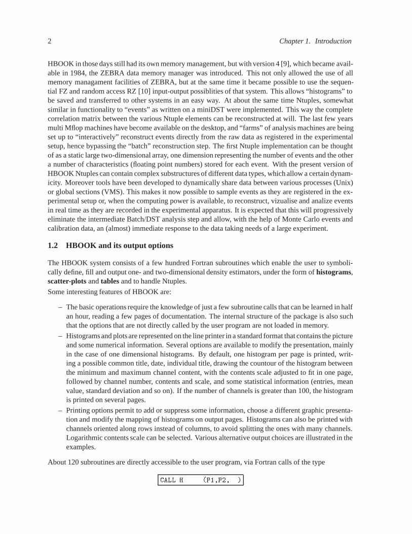
2 Chapter 1. Introduction
HBOOK in those days still had its own memory management, but with version 4 [9], which became avail-able in 1984, the ZEBRA data memory manager was introduced. This not only allowed the use of allmemory managament facilities of ZEBRA, but at the same time it became possible to use the sequen-tial FZ and random access RZ [10] input-output possiblities of that system. This allows “histograms” tobe saved and transferred to other systems in an easy way. At about the same time Ntuples, somewhatsimilar in functionality to “events” as written on a miniDST were implemented. This way the completecorrelation matrix between the various Ntuple elements can be reconstructed at will. The last few yearsmulti Mflop machines have become available on the desktop, and “farms” of analysis machines are beingset up to “interactively” reconstruct events directly from the raw data as registered in the experimentalsetup, hence bypassing the “batch” reconstruction step. The first Ntuple implementation can be thoughtof as a static large two-dimensional array, one dimension representing the number of events and the othera number of characteristics (floating point numbers) stored for each event. With the present version ofHBOOK Ntuples can contain complex substructures of different data types, which allow a certain dynam-icity. Moreover tools have been developed to dynamically share data between various processes (Unix)or global sections (VMS). This makes it now possible to sample events as they are registered in the ex-perimental setup or, when the computing power is available, to reconstruct, vizualise and analize eventsin real time as they are recorded in the experimental apparatus. It is expected that this will progressivelyeliminate the intermediate Batch/DST analysis step and allow, with the help of Monte Carlo events andcalibration data, an (almost) immediate response to the data taking needs of a large experiment.
1.2 HBOOK and its output options
The HBOOK system consists of a few hundred Fortran subroutines which enable the user to symboli-cally define, fill and output one- and two-dimensional density estimators, under the form of histograms,scatter-plots and tables and to handle Ntuples.
Some interesting features of HBOOK are:
– The basic operations require the knowledge of just a few subroutine calls that can be learned in halfan hour, reading a few pages of documentation. The internal structure of the package is also suchthat the options that are not directly called by the user program are not loaded in memory.
– Histogramsand plots are represented on the line printer in a standard format that contains the pictureand some numerical information. Several options are available to modify the presentation, mainlyin the case of one dimensional histograms. By default, one histogram per page is printed, writ-ing a possible common title, date, individual title, drawing the countour of the histogram betweenthe minimum and maximum channel content, with the contents scale adjusted to fit in one page,followed by channel number, contents and scale, and some statistical information (entries, meanvalue, standard deviation and so on). If the number of channels is greater than 100, the histogramis printed on several pages.
– Printing options permit to add or suppress some information, choose a different graphic presenta-tion and modify the mapping of histograms on output pages. Histograms can also be printed withchannels oriented along rows instead of columns, to avoid splitting the ones with many channels.Logarithmic contents scale can be selected. Various alternative output choices are illustrated in theexamples.
About 120 subroutines are directly accessible to the user program, via Fortran calls of the type
CALL H������P��P�����
1.3. What you should know before you start 3
This is the only interface between a Fortran program and the dynamic data structure managed by HBOOK,which thus remains hidden from the average user.
The functionality of HBOOK
The various user routines of HBOOK can be subdivided by functionality as follows:
Booking Declare a one- or two-dimensional histogram or a Ntuple.
Projections Project two-dimensional distributions onto both axes.
Ntuples Way of writing micro data-summary-files for further processing. Thisallows projections of individual variables or correlation plots. Selectionmechanisms may be defined.
Function representation Associates a real function of 1 or 2 variables to a histogram.
Filling Enter a data value into a given histogram, table or Ntuple.
Access to information Transfer of numerical values from HBOOK-managed memory to For-tran variables and back.
Arithmetic operations On histograms and Ntuples.
Fitting Least squares and maximum likelihood fits of parametric functions tohistogramed data.
Monte Carlo testing Fitting with finite Monte Carlo statistics.
Differences between histograms Statistical tests on the compatibility in shape between histograms us-ing the Kolmogorov test.
Parameterization Expresses relationships between as linear combinations of elementaryfunctions.
Smoothing Splines or other algorithms.
Random number generation Based on experimental distributions.
Archiving Information is stored on mass storage for further reference in subsequentprograms.
Editing Choice of the form of presentation of the histogramed data.
1.3 What you should know before you start
The basic data elements of HBOOK are the histogram (one- and two-dimensional) and the Ntuple. Theuser identifies his data elements using a single integer. Each of the elements has a number of attributesassociated with it.
The package is organised as part of a library, from which at load time unsatisfied externals are searchedand loaded. In this way only those subroutines actually used will be loaded, therefore minimising thespace occupied in memory by the code. Unfortunately, given the way Fortran works and although thepackage is structured as much as possible in the sense of selective loading, some unused subroutines willusually be present.

4 Chapter 1. Introduction
HBOOK uses the ZEBRA [10] data structure management package to manage its memory (see chapter 8).The working space of HBOOK is an array, allocated to the labelled common �PAWC�. In ZEBRA termsthis is a ZEBRA store. It is thus necessary to reserve as many locations as required with a declarativestatement in the main program. The actual length of the common is defined most safely via a PARAMETERstatement, as shown below:
PARAMETER �NWPAWC � �����
COMMON �PAWC� HMEMOR�NWPAWC�
Furthermore HBOOK must be informed of the storage limit via a call to HLIMIT. This is discussed indetail in section 8.2 on page 158. In the case above this would correspond to
CALL HLIMIT(NWPAWC)
At execution time, when histograms are booked, they are accomodated in common �PAWC� in bookingorder, up to the maximum size available.
Note that a call to HLIMITwill automatically initialise the ZEBRA system via a call to the routineMZEBRA.If ZEBRA has already been initialised, (MZEBRA has already been called), then HLIMIT should be calledwith a negative number indicating the number of words required, e.g.
CALL HLIMIT(-NWPAWC)
1.3.1 HBOOK parameter conventions
Histogram or Ntuple Identiers
Histograms and Ntuples in HBOOK are identified by a positive or negative integer. Thus the histogramidentifier ID � � is illegal at booking time. However it is a convenient way to specify that the option oroperation applies to all known histograms in the current working directory (e.g. output, input, printing).All routines for which a zero identifier is meaningful are mentioned explicitly.
Parameter types
In agreement with the Fortran standard, when calling an HBOOK routine the type of each parameter mustcorrespond to the one described in the routine’s calling sequence in this manual. Unless explicitly statedotherwise, parameters whose names start with I� J� K� L� M or N are integer, the rest real, with theexception of those beginning with the string CH, which correspond to character constants.
Data packing
All booking commands that reserve space for histograms or plots require the “packing” parameter VMX. Itcorresponds to the estimated maximum populationof a single bin, on the basis of which a suitable numberof bits per channel will be allocated. This allows several channels to be packed in one machine word, andthus to require less storage space (at the expense of packing and unpacking processing time). A valueVMX���� signals that no packing is to be performed and that each histogram channel will occupy onemachine word.

1.4. A basic example 5
1.4 A basic example
Below a simple example is given describing how to use HBOOK for booking, filling and printing simplehistograms. After telling HBOOK the length of the �PAWC� common block to be �����words with a callto HLIMIT, a global title to appear on all histograms is specified by calling HTITLE. Next a 100 bin one-dimensional histogram with identifier 10 is booked with a call to HBOOK�, followed by the booking usinga call to HBOOK� of a two-dimensional histogram with identifier 20 and consisting of 100 times 40 cells.The DO-loop labelled 10 fills the one-dimensional histogram 10, while the nested DO loops labelled 20and 30 look after filling the two-dimensional histogram 20. In both cases a call is made to routine HFILL.Finally a call to HISTDO writes an index with information about all histograms as well as a lineprinterrepresentation of the histograms on standard output.
Example of how to produce simple histograms
PROGRAM HSIMPLE
PARAMETER �NWPAWC � ������
COMMON�PAWC�H�NWPAWC�
��������������������������������������������
CALL HLIMIT�NWPAWC�
Set global title
CALL HTITLE��EXAMPLE NO � ���
Book ��dim histogram and scatter�plot
CALL HBOOK�����EXAMPLE OF ��DIM HISTOGRAM�������������
CALL HBOOK�����EXAMPLE OF SCATTER�PLOT������������������
Fill ��dim histogram
DO �� I�����
W��� MOD�I���
CALL HFILL���FLOAT�I�������W�
�� CONTINUE
Fill scatter�plot
X�������
DO � I�����
X�X�����
DO �� J����
Y�J
IW�MOD�I��� MOD�J���
IWMAX�J�MOD�I������
IF�IW�GT�IWMAX�IW��
CALL HFILL���XYFLOAT�IW��
�� CONTINUE
� CONTINUE
Print all histograms with an index
CALL HISTDO
END

6 Chapter 1. Introduction
Output Generated
EXAMPLE NO � �
������������������������������������������������������������������������������������������������������������������������������ �� HBOOK HBOOK CERN VERSION ���� HISTOGRAM AND PLOT INDEX �������� �� ������������������������������������������������������������������������������������������������������������������������������� �� NO TITLE ID B�C ENTRIES DIM NCHA LOWER UPPER ADDRESS LENGTH �� ������������������������������������������������������������������������������������������������������������������������������� �� �� � EXAMPLE OF �DIM HISTOGRAM � �� � � X � ��E�� ���E�� ����� ��� �� �� �� � EXAMPLE OF SCATTERPLOT � � � X � �E� ��E�� ����� �� �� Y � ��E�� ���E�� ����� ��� �� ������������������������������������������������������������������������������������������������������������������������������
MEMORY UTILISATION
MAXIMUM TOTAL SIZE OF COMMON �PAWC� �
EXAMPLE NO � �EXAMPLE OF �DIM HISTOGRAM
HBOOK ID � � DATE �������� NO � �
� �� �� I I I I�� II II II II�� I I I I I I I I� I I I I I I I I�� I I I I I I I I�� I I I I I I I I�� I I I I I I I I�� I I I I I I I I� I I I I I I I I�� I I I I I I I I�� I I I I I I I I�� I I I I I I I I�� I I I I I I I I� I I I I I I I I� I I I I I I I I� I I I I I I I I� I I I I I I I I� I I I I I I I I I I I I I I I I� I I I I I I I I� I I I I I I I I� I I I I I I I I� I I I I I I I I
CHANNELS � �� � � � � � � � � � ���� �������� �������� �������� �������� �������� �������� �������� �������� �������� ����
CONTENTS � ��������������� ��������������� ��������������� ���������������� ���� �������� �������� ���� �������� �������� ���� �������� �������� ���� �������� ����������
LOWEDGE � �� ���������������������������������������� ������������������������������������������ ���� �������� �������� �������� �������� �������� �������� �������� �������� �������� ����
� ENTRIES � � � ALL CHANNELS � ���E� � UNDERFLOW � �E� � OVERFLOW � �E�� BIN WID � ��E�� � MEAN VALUE � � ���E�� � R � M � S � ��� �E��

1.4. A basic example 7
EXAMPLE NO � �
EXAMPLE OF SCATTERPLOT
HBOOK ID � � DATE �������� NO � �
CHANNELS � U � O� N � � � � � � � � V� D ���� �������� �������� �������� �������� �������� �������� �������� �������� �������� ���� E������������������������������������������������������������������������������������������������������������
OVE � � OVE� � � ��� � �IR� �IR� �IR� �IR� � ���� � �GO�� �GO�� �GO�� �GO�� � ���� � �ELS� �ELS� �ELS� �ELS� � ���� � �CIOU� �CIOU� �CIOU� �CIOU� � ��� � AFKPU� AFKPU� AFKPU� AFKPU� � � �� � ��CGKOS� ��CGKOS� ��CGKOS� ��CGKOS� � ���� � ���CFILORU ���CFILORU ���CFILORU ���CFILORU � ���� � ����ACEGIKMOQS ����ACEGIKMOQS ����ACEGIKMOQS ����ACEGIKMOQS � ���� � ���� ����ABCDEFGHIJK ���� ����ABCDEFGHIJK ���� ����ABCDEFGHIJK ���� ����ABCDEFGHIJK � ��� � � ��� � �IR �IR �IR �IR � ���� � �GO� �GO� �GO� �GO� � ���� � �ELS �ELS �ELS �ELS � ���� � �CIOU �CIOU �CIOU �CIOU � ��� � AFKP AFKP AFKP AFKP � � �� � ��CGKO ��CGKO ��CGKO ��CGKO � ���� � ���CFILO ���CFILO ���CFILO ���CFILO � ���� � ����ACEGIK ����ACEGIK ����ACEGIK ����ACEGIK � ���� � ���� ����ABCDEF ���� ����ABCDEF ���� ����ABCDEF ���� ����ABCDEF � ��� � � ��� � �I �I �I �I � ���� � �GO �GO �GO �GO � ���� � �EL �EL �EL �EL � ���� � �CI �CI �CI �CI � ��� � AFK AFK AFK AFK � � �� � ��CG ��CG ��CG ��CG � ���� � ���CF ���CF ���CF ���CF � ���� � ����ACE ����ACE ����ACE ����ACE � ���� � ���� ����A ���� ����A ���� ����A ���� ����A � ��� � � �� � � � � � � �� � �G �G �G �G � �� � �E �E �E �E � �� � �C �C �C �C � � � A A A A � � � �� �� �� �� � �� � ��� ��� ��� ��� � �� � ���� ���� ���� ���� � �� � ���� ���� ���� ���� � �
UND � � UND������������������������������������������������������������������������������������������������������������
LOWEDGE ���������������������������������������� ���������������������������������������� ���� �������� �������� �������� �������� �������� �������� �������� �������� �������� ����
� I I� ENTRIES � � PLOT II� SATURATION AT� �� I ����I� SCALE ������������ A�B� STATISTICS II� STEP � �� � MINIMUM�� I I

8 Chapter 1. Introduction
1.5 HBOOK batch as the first step of the analysis
MAINFRAME WORKSTATION
Batch Job
HBOOK
ZEBRATapes
Raw Data
DST
Interactive DataAnalysis with PAW
KUIPHPLOT
HBOOK
HIGZZEBRA
SIGMA
COMIS
MINUITManyTapes
RZ Files
High qualitygraphics output
Interactive accessvia RLOGIN
or file transferusing ZFTP
Figure 1.1: Schematic presentation of the various steps in the data analysis chain
Although it is possible to define histograms interactively in a PAW session, and then read the (many thou-sands of) events, in general for large data samples the relevant variables are extracted from the Data Sum-mary Files or DSTs and stored in histograms or an Ntuple. Histograms require to make a certain choiceas to the range of values for the plotted parameter, because the binning, or the coarseness, of the distribu-tion has to be specified when the histogram is defined (booked). Also only one- and two-dimensional his-tograms are possible, hence the correlations between various parameters can be difficult to study. Hencein many cases it is more appropriate to store the value of the important parameters for each event in anNtuple. This approach preserves the correlation between the parameters and allows selection criteria tobe applied on the (reduced) data sample at a later stage.
In general, the time consuming job of analysing all events available on tape is run on a mainframe orCPU server, and the important event parameters are stored in a Ntuple to allow further detailed study.For convenience the Ntuple can be output to disk for each run, and then at a later stage the Ntuples canbe merged in order to allow a global interactive analysis of the complete data sample (see Figure 1.1).
A typical batch job in which data are analysed offline and some characteristics are stored in HBOOK isshown in Figure 1.2. HBOOK is initialised by a call to HLIMIT, which declares a length of 20000 wordsfor the length of the �PAWC� dynamic store. Then the one- and two- dimensional histograms 110 and 210are filled respectively according to the functions HTFUN� and HTFUN� and the histograms are output to anewly created file HTEST�DAT. The output generated by the program is shown in Figure 1.3.

1.5. HBOOK batch as the first step of the analysis 9
PROGRAM HTESTPARAMETER �NWPAWC�������COMMON�PAWC�H�NWPAWC�EXTERNAL HTFUN��HTFUN�
�CALL HLIMIT�NWPAWC�
� Book histograms and declare functionsCALL HBFUN�������Test of HRNDM�����������HTFUN��CALL HBOOK�������Filled according to HTFUN����������������CALL HBFUN�������Test of HRNDM������������������HTFUN��CALL HSCALE�������CALL HBOOK�������Filled according to HTFUN������������������ ��
� Fill histogramsDO �� I��������
X�HRNDM������CALL HFILL�����X�����CALL HRNDM������X�Y�CALL HFILL�����X�Y���
�� CONTINUE� Save all histograms on file HTESTDAT
CALL HRPUT����HTESTDAT���N��CALL HDELET�����CALL HDELET�����CALL HPRINT���ENDFUNCTION HTFUN��X�Y�
� Twodimensional gaussianHTFUN��HTFUN��X��HTFUN��Y�RETURNENDFUNCTION HTFUN��X�
� Constants for gaussiansDATA C��C�������DATA XM��XM��� ����DATA XS��XS����������
� Calculate the gaussiansA�������XXM���XS�����A�������XXM���XS�����X��C�X��C�IF�ABS�A��GT������X��C��EXP�A��IF�ABS�A��GT������X��C��EXP�A��
� Return function valueHTFUN��X��X�RETURNEND
Figure 1.2: Writing data to HBOOK with the creation of a HBOOK RZ file
Filled according to HTFUN1
HBOOK ID = 110 DATE 02/09/89 NO = 2
340 -330 I -320 I I310 I I300 I-I-290 --I I280 -I I-270 I I260 I I250 -I I-240 I I230 -I I220 I I-210 -I I200 I I -190 I I-I180 -I I170 I I -160 I I - -I- -150 I I- I --I I- -I -140 I I- -I--I I-II-I-130 --I I- -I I120 I I - -I I110 I I I-I I--100 I I- -I I
90 -I I- -I I----80 -I I --I I-70 I I -I I60 -I I-- - I I- -50 -I I-- ----I-I I-I-40 I I-I I---30 --I I--20 --I I --10 -------I I-II--
CHANNELS 100 0 110 0 1 2 3 4 5 6 7 8 9 0
1 1234567890123456789012345678901234567890123456789012345678901234567890123456789012345678901234567890
CONTENTS 100 111222222323222211111 111111111111111111111110 1 12224578227034888392975189442985544344445467789101235335456543453430088887545443322111
1. 22345055038484428230601947383077660674994445157562761227948358021717653142735611669210337304276
LOW-EDGE 1. 111111111122222222223333333333444444444455555555556666666666777777777788888888889999999999*10** 1 0 0123456789012345678901234567890123456789012345678901234567890123456789012345678901234567890123456789
* ENTRIES = 10000 * ALL CHANNELS = 0.1000E+05 * UNDERFLOW = 0.0000E+00 * OVERFLOW = 0.0000E+00* BIN WID = 0.1000E-01 * MEAN VALUE = 0.4846E+00 * R . M . S = 0.2199E+00
Fill according to HTFUN2
HBOOK ID = 210 DATE 02/09/89 NO = 4
CHANNELS 100 0 110 0 1 2 3 4 5 6 7 8 9 0
1 1234567890123456789012345678901234567890123456789012345678901234567890123456789012345678901234567890********************************************************************************************************
OVE * * OVE.975 * * 40.95 * ++ 2 2 2++ +3 + ++ + + 2+ 3 2 + 2++++ + 2 + * 39.925 * + + 2 ++ 32+++ +22 22+ +++ + + + + 22+2+++ +2++ + + + * 38.9 * 223 +3+ +3 3++333223 +2 2 + + ++2+ + 232+322 2+++ +24+ + * 37.875 * + ++ +2++++ 342533 443224++2 2 + + ++23 + +42+3222233+++3+++2 22+ ++ + + + * 36.85 * ++ + 5+35+3333483475 65+2+ + ++ + +33+3 +2 +2335222+235 522 24+ ++ 2 * 35.825 * ++ 2+2 558335876736583+ 2 +2+ + + 3 224+533623+35252+54 32+452++3 332 +++++ * 34.8 * ++ + 532 656562546C8A88936324332+ +2+23 +332+2236433657234455556+4635+222 +23 +3 + * 33.775 * +2 33 375B7274C6A66A782+323++2+23 +5++3+5222256768365258276374+86334+ 32 +++ + * 32.75 * + 2+ 2 45523786A79FB98B6AD4855224+ + ++23323+5755552468283746644543 443324 5223++ 2 * 31.725 * + ++4+22+637A785B8BBBA6B4656922++ 2 23 24 2+5464+435552843286C6246623636+3+ 2 3 2 3+2 * 30.7 * + 22 +2 735ABCA89G8C8A6DA5765+3+322 2+2++52234445475+355864768724+B74632+23 +3 3+ + * 29.675 * 23 +4+3364HBBAFCFCBB98945C7933++ 2 5+3 +4225243752 75787896C367+475443+32242422 2 + * 28.65 * + + ++5+3795498GAC96CB9A79E6645 34 3+3 ++24537234424532777657445+4746235+2+3++ 4+2 2 * 27.625 * + 3 647774A9CE67G99BAB6B233233 4+ 2 322 42 44364+657735+735736733+4+23234 +++++2 + * 26.6 * + ++3+342233874B8C966896565+5242+5 +2+++++2+5225+42544535456A265357253+2222+ 2+2++ + +2 * 25.575 * ++ + +5 74535525677984573453422 +2 ++ 2 +++4+2 3526525235+4243342+32+ 23 2+ * 24.55 * ++ +226+584568349865+433 +2222 + ++ +4444352326542332823+444332 +2 2 + + * 23.525 * ++++2+65436+3A753535+22+++2+++ ++ + ++2 +2 ++4++2+ 224224+32 2+ ++++ 2 + * 22.5 * 22 4+23+6425 84543+++42 +2 +++2 2 + 2+2+ 3+ 24++2334223+ 223 +2 + + * 21.475 * + +5334+7333+22 ++2+ + 3+ 2 +4 +32 2 222+2 + 33++ 222 + +3++ + * 20.45 * + 433244397 2++23232+ 24 +2 ++ ++2+ 2+ +2+33 ++4 +3 ++2+3 + + * 19.425 * + ++ 2+ 22+24636432646+5+322 4 +++ + 2++ ++ +22+533+3++3+ +432 +322++2+ 2+ ++ + * 18.4 * +++3237549588A9725H724545++33+33 + + 2 24 4 +A4633 39 25636343322+82++ ++ + +2+ + * 17.375 * +++3+374879CCCADLD48996CE54365232 +2+2342347+563264636547B47925542444434+2+322 2+ +2 * 16.35 * +++ +4637549EC87D8IHDICI9B754655432++23233+2554368886H68B9667889677A635C+4+223333+22 + * 15.325 * + ++++ 2445949CHHDFNHJRHIHKLDD5DC3545422233 24564875549A8E7899B4F4BC3CA7E597842+67242+++++ * 14.3 * ++++++2667889EDFEHULQHI*IKFIFA878666336+6+48526B79777BCCEBBAEEED58E96997A4674763463++++ 2+ * 13.275 * + ++++ 3546898BEMPNIURPH*NOECDC8958E442+3542+68554B37466AAGCEEACAC7A476599962365 343++2 +2 * 12.25 * + 2344658A9DAJPLDENQGDHJEEBAA93 +3225322+4259A576784DA9B98B56A85CD859797A5843523223+ 22 * 11.225 * 3 256778BA6CEJGIEAICGCHA4A242+43+++52427545466927A78866BB66795655763454656 2 3 +++ * 10.2 * +2++4357A69BC88AAFAA5665432+434 +++ ++++343233668554584442CA7664745+4++34+++2 + +++ * 9.175 * + 3 3436344766755264526++3 2+ + ++ +42 22 2+32345++353562 34 33+++4 +3 +++ + * 8.15 * 2+ + +3+44+262542+4225 232 ++++ 222 + 2+ +23+242 32+222 2++342 22 22+ 2 + * 7.125 * + +2 +++22+32+ 3+++2 + +42 + 2+ + + 2+ + + ++ * 6.1 * + + + +2+ ++ + +2+ + ++ +++ + * 5.075 * + 2 + + + + * 4.05 * + * 3.025 * + * 2
* * 1UND * * UND
********************************************************************************************************LOW-EDGE 0 0000000000111111111122222222223333333333444444444455555555556666666666777777777788888888889999999999
0 0123456789012345678901234567890123456789012345678901234567890123456789012345678901234567890123456789
* I I* ENTRIES = 10000 PLOT ---------I---------I---------* SATURATION AT= 31 I 9991 I* SCALE .,+,2,3,.,., A,B, STATISTICS ---------I---------I---------* STEP = 1 * MINIMUM=0 I I
Figure 1.3: Output generated by job HTEST

10 Chapter 1. Introduction
1.5.1 Adding some data to the RZ file
A second run using program HTEST� below shows how to add some data to the HBOOK RZ file created inthe job HTEST (Figure 1.2). After opening the file HTEST�DAT, created in the previous run, in update mode(�U� option) with the name EXAM�, a new directory NTUPLE is created, known as ��EXAM��NTUPLE asseen in the output of HLDIR command at the end of the output. One-dimensional (10) and two-dimensional(20) histograms and an Ntuple (30) are booked. Each Ntuple element or “event” is characterised by threevariables (labelled �X�, �Y� and �Z�). The Ntuple data, when the initial size of ����words is exhausted,will be written to the directory on disk specified in the call to HBOOKN, i.e. ��EXAM��NTUPLE, and the datain memory are replaced with those newly read. A one- and a two-dimensional projection of X and X�Y
are then made onto histograms 10 and 20 respectively, before they are printed and written on the HBOOKRZ file. At the end the current and parent directories are listed. The contents of the latter shows that thedata written in the first job (HTEST) are indeed still present in the file under the top directory ��EXAM�.The call to RZSTAT shows usage statistics about the RZ file.
Example of adding data to a HBOOK RZ file
PROGRAM HTEST�
PARAMETER �NWPAWC�������
COMMON�PAWC�H�NWPAWC�
DIMENSION X��
CHARACTER � CHTAGS��
DATA CHTAGS�� X �� Y �� Z ��
�����������������������������������������������������
CALL HLIMIT�NWPAWC�
Reopen data base
LRECL � �
CALL HROPEN���EXAM���HTEST�DAT��U�LRECLISTAT�
CALL HMDIR��NTUPLE��S��
CALL HBOOK�����TEST�����������
CALL HBOOK�����TEST���������������
CALL HBOOKN���N�TUPLE����EXAM��NTUPLE�
� ����CHTAGS�
DO �� I�������
CALL RANNOR�AB�
X����A
X����B
X���A A�B B
CALL HFN��X�
�� CONTINUE
CALL HPROJ����������������
CALL HPROJ�����������������
CALL HPRINT���
CALL HROUT��ICYCLE� ��
CALL HLDIR�� �� ��
CALL HCDIR����� ��
CALL HLDIR�� �� ��
CALL RZSTAT�� ����� ��
CALL HREND��EXAM���
END

1.5. HBOOK batch as the first step of the analysis 11
TEST1
HBOOK ID = 10 DATE 02/09/89 NO = 1
280270 - -260 I I -250 - I I I240 - I I-I- I -230 I-I--I I I-I-220 -I I I I-210 I I I I-200 I I-I I-190 - - --I I --180 I-I-I I-II--170 I I160 I I--150 - -I I --140 -I-I I II130 -I I-II-120 -I I-110 --I I--100 --I I
90 I I80 I I----70 --I I-60 -I I--50 ---I I--40 -----I I--30 I I-----20 - ----I I---10 --------I-I I--------
CHANNELS 100 0 110 0 1 2 3 4 5 6 7 8 9 0
1 1234567890123456789012345678901234567890123456789012345678901234567890123456789012345678901234567890
CONTENTS 100 1111111111111112222222222122222211111111111111110 1 1111333334446669000123434878888132522637496233109788775524421007777655443322222111
1. 1266487877127932587516069303434644322909949809367004036056844525243975324963516782565365312194856211
LOW-EDGE --------------------------------------------------1. 3222222222222222211111111111111111 1111111111111111122222222222222220 09887765544322110998876655433221009987766544332110001123344566778990012233455667889901122344556778890 0482604826048260482604826048260482604826048260482606284062840628406284062840628406284062840628406284
* ENTRIES = 10000 * ALL CHANNELS = 0.9969E+04 * UNDERFLOW = 0.1200E+02 * OVERFLOW = 0.1900E+02* BIN WID = 0.6000E-01 * MEAN VALUE =-0.3907E-02 * R . M . S = 0.9857E+00
TEST�HBOOK ID � � DATE ������ NO � �CHANNELS � U � � � O
� N ���� �������� �������� ���� V��������������������������������������
OVE � � �� �������� ��� � OVE��� � �� � �� � � � � ���� � � �� ������ �� � � ����� � �� �������� ��� � � ����� � � � ��������� ������� � � ��� � � ������� ��A� ���� � � ����� � � �� ��EBCDAA �� � �� � � � ��� � ������CC�JFO�F��C�������� � ����� � ������AAGJJMEMIDFG������� � � ����� � ������BBJGMQOPWNICCGI������� � � ��� � �� � BGOMTSX�VYTJMCFA� ��� � ���� � ������DHSRUX����VXRQJC ��� � � ��� � � �� CBEKLZ��������MXGGCI���� � � ���� � � �����BN�U���������YOIFB��� � ���� � � �����CCLR������������OIHA����� � � ��
� � ����ECX�T�����������YKPC��� � � �� �� � � ����D�LDS��X��������ZUMGC ��� � � � �� � � ����CAHSSX���������UMK� D� � � � �� �� � ����AAKML�V����������IIH������ � � �� �� � ��� � CLJL�X������Z�TL�H���� � � �� � � � � �����EMLN����Q�ULLQMABB���� � � �� ��� � � �����BDIUS�P���TTUNBDA � �� � � ��� � � � � ����E�KKNWUNRIHJCEA������ � � � ��� � ������BCMJIGOIKEIAAD������ � � � ��� � � � ������ �AA�HGJACB���������� � � � � � � ���� ��EDC �������� � � ��� � � � ���������� ��������� ��� � ��� � � ����� ��� ����� � � � ��� � �� � ������������ � � � � ��� � � ���������� � � � � � �� �� �� � ���� � � �
UND � � � �� ����� � � UND��������������������������������������
LOWEDGE �� ����������� ���������� ������������������������
� I �� I� ENTRIES � � PLOT II� SATURATION AT� � �� I ���� I ��� SCALE ������������ A�B� STATISTICS II� STEP � � � MINIMUM� I �� I
NTUPLE ID� � ENTRIES� ����� N�TUPLE
Var numb Name Lower Upper
� X ��������E��� �������E���
� Y ��������E��� ������E���
Z ��������E��� ��������E���
���� Directory � ��EXAM��NTUPLE
� �N� N�TUPLE
�� ��� TEST�
�� ��� TEST�
���� Directory � ��EXAM�
��� ��� Test of HRNDM�
��� ��� Filled according to HTFUN�
��� ��� Test of HRNDM�
��� ��� Fill according to HTFUN�
NREC NWORDS QUOTA��� FILE��� DIR� NAME
� ���� ��� ��� ��EXAM��NTUPLE
�� ���� ��� ��� ��EXAM�
Figure 1.4: Adding data to a HBOOK RZ file

12 Chapter 1. Introduction
1.6 HPLOT interface for high quality graphics
hplot is a package of Fortran subroutines for producing hbook output suitable for graphic devices or inPostScript. It is designed to produce drawings and slides of a quality suitable for presentations at confer-ences and scientific publications. It does not produce all the numerical information of the HBOOK outputroutines. It is not restricted by the line printer’s poor resolution and unique character sets but it uses thefull graphics capabilities of the targeted output device.
HPLOT can access an HBOOK data structure and transform it into drawings using the HIGZ graphicspackage. Some of the available options are :
– Predefined ISO standard paper size (A4, A3, etc.), horizontal or vertical orientation, with suitablemargins. Other sizes are also possible.
– Combination of several plots on the same page, either by windowing or superimposition, or both,with different symbols to distinguish them.
– Titles on the axes and text anywhere on the picture, using various fonts, containing, e.g., Greek orspecial characters.
– Three-dimensional surface representations for two-dimensional histograms (with hidden-line andhidden-surface removal).
– Colour (if the hardware allows it), hatching, grey levels,. . . .
As a simple example of the use of HPLOT let us consider a program similar to the one in Figure 1.4.After opening a file on unit 10 to write the metafile output (Fortran OPEN statement), we book, then fill theNtuple projections, and finally plot them. The call to HPLINT initialises HPLOT and HPLCAP redirects themetafile output to unit 10. The parameters given to HPLOT instruct the program to output all histogramsin the current working directory to the metafile using “standard” option, while HPLEND closes the metafile.See the HPLOT user’s guide [2] for more details. The result of the job and the resulting PostScript filecan be compared to the “lineprinter” output in Figure 1.4.
Example of a simple HPLOT program
PROGRAM HPTEST
COMMON�PAWC�H�������
DIMENSION X��
CHARACTER � CHTAGS��
DATA CHTAGS�� X �� Y �� Z ��
�������������������������������������������������������������
CALL HLIMIT�������
Reopen data base
OPEN�UNIT���file��hplot�meta�form��formatted�status��unknown��
CALL HBOOK�����TEST�����������
CALL HBOOK�����TEST���������������
CALL HBOOKN���N�TUPLE�� �����CHTAGS�
DO �� I�������
CALL RANNOR�AB�
X����A
X����B
X���A A�B B
CALL HFN��X�
�� CONTINUE

1.6. HPLOT interface for high quality graphics 13
CALL HPROJ����������������
CALL HPROJ�����������������
CALL HPLINT���
CALL HPLCAP�����
CALL HPLOT��� �� ���
CALL HPLEND
CALL HINDEX
END
Output Generated
Version ����� of HIGZ started������������������������������������������������������������������������������������������������������������ �� HBOOK HBOOK CERN VERSION ���� HISTOGRAM AND PLOT INDEX ������ �� ������������������������������������������������������������������������������������������������������������� �� NO TITLE ID B�C ENTRIES DIM NCHA LOWER UPPER ADDRESS LENGTH �� ������������������������������������������������������������������������������������������������������������� �� �� � TEST� � �� � � X � ��E�� ��E�� ����� ��� �� �� �� � TEST� � � � � X � ��E�� ��E�� ���� ��� �� Y � ��E�� ��E�� ����� ��� �� �� � NTUPLE � N ����� �� �� �� ������������������������������������������������������������������������������������������������������������
MEMORY UTILISATIONMAXIMUM TOTAL SIZE OF COMMON �PAWC� �
Output generated by HPLOT on printer with graphics capabilities

Chapter 2: One and two dimensional histograms – Basics
2.1 Booking
2.1.1 One-dimensional case
CALL HBOOK1 �ID�CHTITL�NX�XMI�XMA�VMX�
Action: Books a one-dimensional histogram.
Input parameter description:
ID histogram identifier, integer non zero
CHTITL histogram title (character variable or constant up to 80 characters)
NX number of channels
XMI lower edge of first channel
XMA upper edge of last channel
VMX upper limit of single channel content (see below).VMX��� means 1 word per channel (no packing).
Special values:
– If XMA�XMI, origin and binwidth are calculated automatically, and one word is reserved per chan-nel.
– Zero (0) is an illegal histogram identifier.
– If the histogram ID already exists it will be deleted and recreated with the new specifications. Awarning message is printed.
– VMX is used to compute the number of bits to be allocated per histogram channel. If VMX��� thenone full word is reserved per channel. When filling a histogram with weights the latter are truncatedto the nearest integer unless one full word is reserved per channel (i.e. VMX � ��). Filling withnegative weights will give meaningless results unless one word per channel has been allocated.Automatic calculation of limits (XMA�XMI) forces one word per channel.
2.1.2 Two-dimensional case
CALL HBOOK2 �ID�CHTITL�NX�XMI�XMA�NY�YMI�YMA�VMX�
Action: Books a two-dimensional histogram.
Input parameter description:
ID histogram identifier, integer
CHTITL histogram title (character variable or constant up to 80 characters)
NX number of channels in X
14
2.2. Filling 15
XMI lower edge of first X channel
XMA upper edge of last X channel
NY number of channels in Y
YMI lower edge of first Y channel
YMA upper edge of last Y channel
VMX maximum population to store in 1 cell.
Remarks:
– Similar to HBOOK1, apart from automatic binning.
– By default, a 2-dimensional histogram will be printed as a scatterplot.
– If the optionTABL is selected via CALL HIDOPT�ID��TABL�� the 2-dimensional histogram will beprinted as a table.
– When editing the table, the number of columnsNCOL used to write the content of one cell depends onthe value of VMX as followsNCOL � ALOG���VMX� � �. When VMX is zero, the contents is printedin 10 columns in floating point format (including sign). If necessary, all contents are multiplied bya power of 10, this number being reported at the bottom of the table.
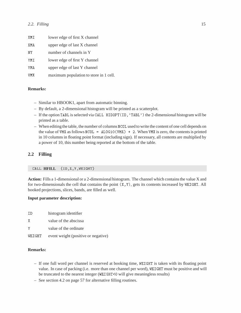
2.2 Filling
CALL HFILL �ID�X�Y�WEIGHT�
Action: Fills a 1-dimensional or a 2-dimensional histogram. The channel which contains the value X andfor two-dimensionals the cell that contains the point �X�Y�, gets its contents increased by WEIGHT. Allbooked projections, slices, bands, are filled as well.
Input parameter description:
ID histogram identifier
X value of the abscissa
Y value of the ordinate
WEIGHT event weight (positive or negative)
Remarks:
– If one full word per channel is reserved at booking time, WEIGHT is taken with its floating pointvalue. In case of packing (i.e. more than one channel per word), WEIGHT must be positive and willbe truncated to the nearest integer (WEIGHT�� will give meaningless results)
– See section 4.2 on page 57 for alternative filling routines.

16 Chapter 2. One and two dimensional histograms – Basics
2.3 Editing
CALL HISTDO
Action: Outputs all booked histograms to the line printer. An index is printed at the beginning specifyingthe characteristics and storage use of each histogram.
Remark:
– If a histogram is empty, a message declares this condition, and the histogram is not printed.
CALL HPRINT �ID�
Action: Outputs a given histogram to the line printer.
ID Histogram identifier.
Remarks:
– CALL HPRINT��� is equivalent to CALL HISTDO apart from not printing the index
– When a histogram is empty a message declares this condition and the histogram is not printed.
Some available booking options are shortly listed below. For a full description see chapter 4.
– Creation of histograms with non-equidistant bins
– Creation of profile histograms
– Rounded scale
– Projections and slices of 2-dimensional histograms
– More statistical information
– Comprehensive booking and filling with user-supplied functions of one or two real variables.
– Dynamic creation of ordinary Fortran arrays (HARRAY)
2.4. Copy, rename, reset and delete 17
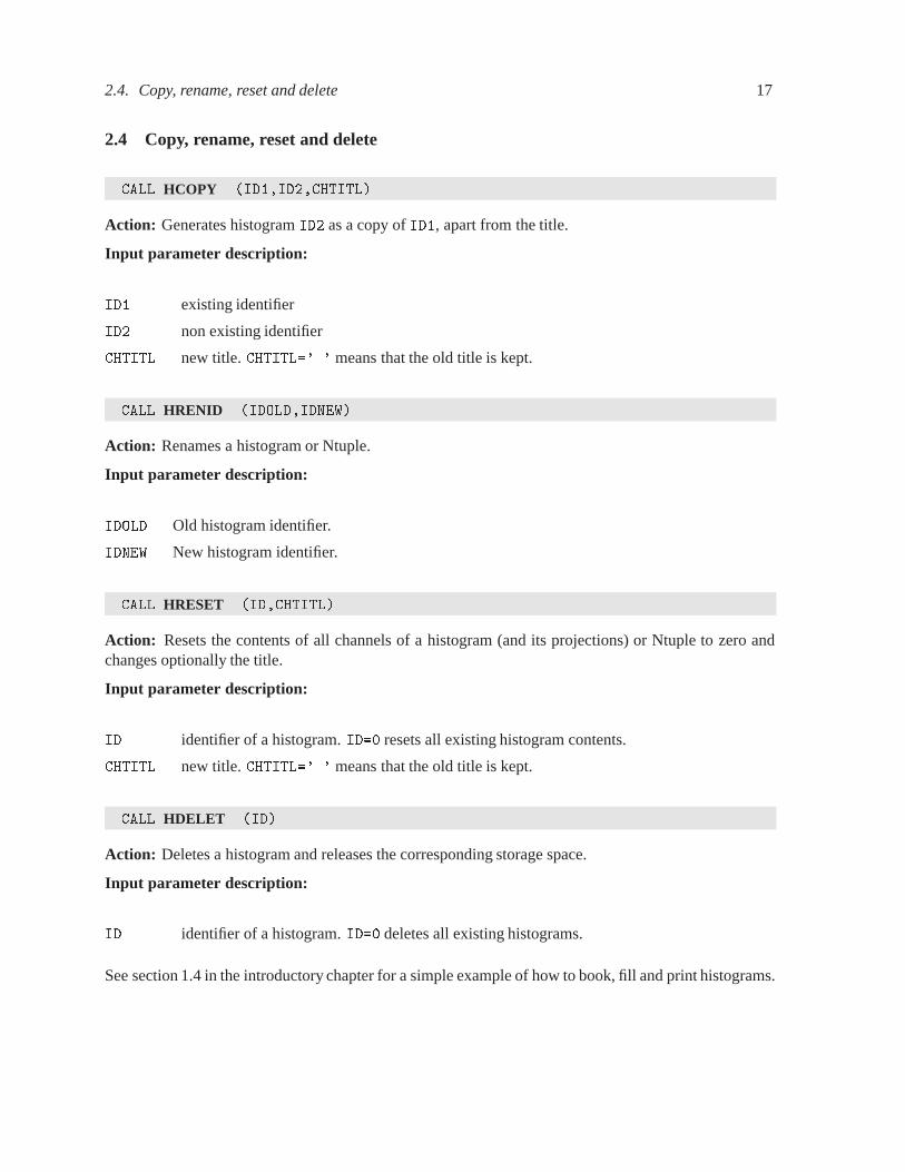
2.4 Copy, rename, reset and delete
CALL HCOPY �ID��ID��CHTITL�
Action: Generates histogram ID� as a copy of ID�, apart from the title.
Input parameter description:
ID� existing identifier
ID� non existing identifier
CHTITL new title. CHTITL�� � means that the old title is kept.
CALL HRENID �IDOLD�IDNEW�
Action: Renames a histogram or Ntuple.
Input parameter description:
IDOLD Old histogram identifier.
IDNEW New histogram identifier.
CALL HRESET �ID�CHTITL�
Action: Resets the contents of all channels of a histogram (and its projections) or Ntuple to zero andchanges optionally the title.
Input parameter description:
ID identifier of a histogram. ID�� resets all existing histogram contents.
CHTITL new title. CHTITL�� � means that the old title is kept.
CALL HDELET �ID�
Action: Deletes a histogram and releases the corresponding storage space.
Input parameter description:
ID identifier of a histogram. ID�� deletes all existing histograms.
See section 1.4 in the introductory chapter for a simple example of how to book, fill and print histograms.

Chapter 3: Ntuples
To introduce the concept of Ntuples, let us consider the followingexample. A Data Summary Tape (DST)contains 10000 events. Each event consists of many variables (say NVAR����) for which we would liketo make some distributions according to various selection criteria.
One possibility is to create and fill 200 histograms on an event-by-event basis while reading the DST.An alternative solution, particularly interesting during interactive data analysis with the data presentationsystem paw [3], is to create one Ntuple. Instead of histograming the 200 variables directly, and thereforelosing the exact values of the variables for each event and their correlations, the variables are first storedin an Ntuple. (One can of course fill the histograms at the same time!) An Ntuple is like a table wherethe 200 variables mentioned above are the columns and each event is a row. The storage requirement isproportional to the number of columns in one event and can become significant for large event samples.An Ntuple can thus be regarded as a standard way of storing a DST.
Once the events are stored in this form, it becomes easy, in particular with paw, to make 1- or more-dimensional projections of any of the NVAR variables of the events and to change the selection mecha-nisms, or the binning and so on. Before running the system on a large number of events, the selectionmechanisms can be rapidly tested on a small sample.
3.1 CWN and RWN – Two kinds of Ntuples
In a Row-Wise-Ntuple (RWN) the elements of each row, usually corresponding to an individual event, arestored contiguously in an HBOOK RZ file. This storage method is similar to that of a conventional DST,where events are stored sequentially and it is particularly suited for small Ntuples (up to a few Mbytes),with only a few columns. You can even use an RWN for larger Ntuples (up to about 20 Mbytes) when youknow you want to reference almost all columns in your query commands. A RWN should not be used ifthere are more than about 100 columns, or when your queries only references a small number of columns.A RWN can only contain floating point data. It is created with HBOOKN and filled with HFN. Routines HGN,HGNF are used to retrieve information about one row.
Figure 3.1 shows schematically how a RWN is laid out in memory, row after row. The buffer size in mem-ory NWBUFF is specified as the primary allocation parameter NWBUFF of the HBOOKN routine. Of course,you must have reserved sufficient space in the �PAWC� common when calling the HBOOK initializationroutine HLIMIT. The lower line shows how the information is written to an RZ file. The length of the in-put/output buffer LRECL is specified as an argument of the routine HROPEN. It is evident that, if you havea small Ntuple and a lot of memory, you can fit the complete Ntuple in memory, thus speeding up theNtuple operations.
In a Column-Wise-Ntuple (CWN) the elements of each column are stored sequentially. Data in such anNtuple can be accessed in a much more flexible and powerful manner than for a RWN. The CWN storagemechanism has been designed to substantially improve access time and facilitate compression of the data,thereby permitting much larger event samples (several hundreds of Mbytes) to be interactively processed,e.g. using paw. Substantial gains in processing time can be obtained, especially if your queries only ref-erence a few columns. A CWN is not limited to floating point data, but can contain all basic data types(real, integer, unsigned integer, logical or character). A CWN is created with routines HBNT, HBNAME orHBNAMC and filled with HFNT and HFNTB. Information about one row/block/column can be retrieved withroutines HGNT, HGNTB, HGNTV and HGNTF.
18

3.1. CWN and RWN – Two kinds of Ntuples 19
Ntuple Header
x1y1z1t1,x2y2z2t2,x3y3z3t3,...
LRECLNWBUFF
( Header created by HBOOKN)
( Buffer filled by HFN)
HBOOK/RZ direct-access file
Figure 3.1: Schematic structure of a RWN Ntuple
NWBUFF
Ntuple Header
x1x2x3x4x5... y1y2y3y4y5... z1z2z3z4z5... t1t2t3t4t5...
LRECL
( Header created by HBNT, HBNAME)
( Buffers filled by HFNT)
HBOOK/RZ direct-access file
Figure 3.2: Schematic structure of a CWN Ntuple
Figure 3.2 shows the layout of a CWN Ntuple. The buffer size for each of the columns NWBUFFwas set equal to therecord length LRECL (defined with routine HROPEN). A CWN requires a large value for the length of the common�PAWC�, in any case larger than the number of columns times the value NWBUFF, i.e. NWPAWC�NWBUFF�NCOL. Youcan, however, expect important performance improvements by setting the buffer size NWBUFF equal to a multipleof the record length LRECL (via routine HBSET).In both figures, xi, yi, zi, ti, etc. represent the columns of event i.

20 Chapter 3. Ntuples
3.2 Row-Wise-Ntuples (RWN)
3.2.1 Booking a RWN
CALL HBOOKN �ID�CHTITL�NVAR�CHRZPA�NWBUFF�CHTAGS�
Action: Books a RWN in memory or with automatic overflow on an RZ file. Only singleprecision floatingpoint numbers (REAL�� on 32 bit machines) can be stored, no data compression is provided.
Input parameters:
ID Identifier of the Ntuple.
CHTITL Character variable containing the title associated with the Ntuple.
NVAR Number of variables per event (NVAR���)
CHRZPA Character variable containing the path name of a RZ file onto which the contents of the Ntuplecan overflow.
� � Memory resident Ntuples:A bank of NWBUFF words is created. Further banks of the same size are added in alinear chain should additional space be required at filling time.
�RZTOP� Disk resident Ntuples: (recommended)A disk resident Ntuple is created if the CHRZPA argument specifies the top directoryname of an existing RZ file that has already been opened with HROPEN or HRFILE. Abank of length NWBUFF is created, as in the case of memory resident Ntuples. How-ever, each time the bank becomes full it is automatically flushed to the RZ file, ratherthan creating additional banks in memory.
NWBUFF Number of words for the primary allocation for the Ntuple.
CHTAGS Character array of length NVAR, providing a short name (up to eight characters) tagging schemefor each variable.
Example of the declaration of a memory resident RWN
CHARACTER � CHTAGS���
DATA CHTAGS��Px��Py��Pz��Q���NU��
CALL HBOOKN����My first NTUPLE��� �����CHTAGS�
3.2.2 Filling a RWN
CALL HFN �ID�X�
Action: Fills a RWN.
Input parameters:
ID Identifier of the Ntuple.
X Array of dimension NVAR containing the values for the current event.

3.2. Row-Wise-Ntuples (RWN) 21
Memory resident Ntuples
When a RWN is booked, HBOOK reserves space in memory in which to store the data, as specified by theNWBUFF argument of routineHBOOKN. As the RWN is filled by a call to HFN, this space will be successivelyused until full. At that time, a new memory allocation will be made and the process continues.
If this data is then written to disk, it appears as one enormous logical record. In addition, it most casesthe last block of data will not be completely filled thus wasting space.
If one tries to reprocess this RWN at a later date, e.g. with paw, there must be enough space in memoryto store the entire Ntuple. This often gives rise to problems and so the following alternative method isrecommended.
Circular buffer
In an online environment you often want to have the lastN events inside a buffer, so that the experimentcan be monitored continuously. To make it easier to handle this case, you can use routine HFNOV, whichfills a circular buffer in memory with RWN events, and when the buffer is full, overwrites the oldest Ntu-ple.
CALL HFNOV �ID�X�
Action: Fills a circular buffer with RWNs.
Input parameters:
ID Identifier of the Ntuple.
X Array of dimension NVAR containing the values for the current event.
Disk resident Ntuples
Prior to booking the RWN, a new HBOOK RZ file is created using HROPEN. The top directory name ofthis file is passed to routine HBOOKN when the Ntuple is booked.
Filling proceeds as before but now, when the buffer in memory is full, it is written to the HBOOK file andthen reused for the next elements of the Ntuple. This normally results in a more efficient utilisation of thememory, both when the Ntuple is created and when it is reprocessed.
Recommended way of creating a RWN
PROGRAM TEST
PARAMETER �NWPAWC � ������
COMMON�PAWC�PAW�NWPAWC�
CHARACTER � CHTAGS���
DIMENSION EVENT���
EQUIVALENCE �EVENT���X��EVENT���Y��EVENT��Z�
EQUIVALENCE �EVENT���ENERGY��EVENT���ELOSS�
DATA CHTAGS��X��Y��Z��Energy��Eloss��
CALL HLIMIT�NWPAWC�
CALL HROPEN���EXAMPLE��EXAMPLE�DAT��N�����ISTAT�
IF�ISTAT�NE���GO TO ��
CALL HBOOKN����A Row�Wise�Ntuple�����EXAMPLE�����CHTAGS�

22 Chapter 3. Ntuples
CALL HBOOK������Energy distribution�������������
DO �� I�������
CALL RANNOR�XY�
Z�SQRT�X X�Y Y�
ENERGY���� � ��� X
ELOSS���� ABS�Y�
CALL HFN���EVENT�
CALL HFILL����ENERGY�����
�� CONTINUE
CALL HROUT��ICYCLE� ��
CALL HREND��EXAMPLE��
�� CONTINUE
END
When the Ntuple is filled, routine HFN will automatically write the buffer to the directory in the RZ file,which was specified in the call to HBOOKN (the top directory ��EXAMPLE in the example above). If thecurrent directory (CD) is different, HFN will save and later automatically restore the CD.
The Ntuple created by the program shown above can be processed by paw as follows.
Reading an RWN in a PAW session
PAW � Histo�file � example�dat
PAW � Histo�plot ���
PAW � Ntuple�plot ���energy
PAW � Ntuple�plot ���eloss energy���
PAW � Ntuple�plot ���eloss�energy x���and�sqrt�z���
By default HROPEN creates a file that can be extended up to 32000 blocks, i.e. 128 Mbytes for a recordlength LREC of 1024 words. If one wishes to create very large Ntuples, one should make two changes tothe above procedure.
– A large value should be used for the record length of the file, e.g. 8192 words (the maximum onmost machines). N.B. the maximum record length on VMS systems is 8191 words. If accessmode RELATIVE is used, the maximum is 4095 words. This remark does not apply to a CWN, asdescribed later.
– Option Q on HROPEN should be used to override the default number of records allowed.
This can be achieved as by changing the previous call to HROPEN as follows:
Writing very large Ntuple files
COMMON�QUEST�IQUEST�����
CALL HLIMIT��������
Create HBOOK file with the maximum record length ����� bytes�
and maximum number of records �������
IQUEST���� � �����
CALL HROPEN���EXAMPLE��EXAMPLE�DAT��NQ�����ISTAT�
IF�ISTAT�NE���GO TO ��

3.3. More general Ntuples: Column-Wise-Ntuples (CWN) 23
3.3 More general Ntuples: Column-Wise-Ntuples (CWN)
A CWN supports the storage of the following data types: floating point numbers (REAL�� and REAL��),integers, bit patterns (unsigned integers), booleans and character strings.
Data Compression
Floating point numbers, integers and bit patterns can be packed by specifying a range of values or by ex-plicitly specifying the number of bits that should be used to store the data. Booleans are always storedusing one bit. Unused trailing array elements will not be stored when an array depends on an index vari-able. In that case only as many array elements will be stored as specified by the index variable.
For example, the array definitionNHITS�NTRACK�definesNHITS to depend on the index variableNTRACK.When NTRACK is 16, the elements NHITS������� are stored, when NTRACK is 3, only the elements oneto three (NHITS������) are stored, etc.
Storage Model
Column wise storage allows direct access to any column in the Ntuple. Histogramming one column froma 300 column CWN requires reading only 1/300 of the total data set. However, this storage scheme re-quires one memory buffer per column as opposed to only one buffer in total for an RWN. By default thebuffer length is 1024 words, in which case a 100 column Ntuple requires 409600 bytes of buffer space. Ingeneral, performance increases with buffer size. Therefore, one should tune the buffer size (using routineHBSET) as a function of the number of columns and the amount of available memory. Highest efficiencyis obtained when setting the buffer size equal to the record length of the RZ HBOOK file (as specified inthe call to HROPEN). A further advantage of column wise storage is that a CWN can easily be extendedwith one or more new columns.
Columns are logically grouped into blocks (physically, however, all columns are independent). Blocksallow users to extend a CWN with private columns or to group relevant columns together. New blocks caneven be defined after a CWN has been filled. The newly created blocks can be filled using routine HFNTB.For example, a given experiment might define a number of standard Ntuples. These would be bookedin a section of the code that would not normally be touched by an individual physicist. However, with aCWN a user may easily add one or more blocks of information as required for their particular analysis.
Note that arrays are treated as a single column. This means that a CWN will behave like a RWN, withthe addition of data typing and compression, if only one array of NVAR elements is declared. This is notrecommended as one thereby loses the direct column access capabilities of a CWN.
Performance
Accessing a relatively small number of the total number of defined columns results in a huge increasein performance compared to a RWN. However, reading a complete CWN will take slightly longer thanreading a RWN due to the overhead introduced by the type checking and compression mechanisms andbecause the data is not stored sequentially on disk. The performance increase with a CWN will mostclearly show up when using paw, where one typically histograms one column with cuts on a few othercolumns. The advantages of having different data types and data compression generally outweighs theperformance penalty incurred when reading a complete CWN.
24 Chapter 3. Ntuples
3.3.1 Booking a CWN
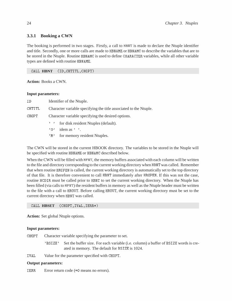
The booking is performed in two stages. Firstly, a call to HBNT is made to declare the Ntuple identifierand title. Secondly, one or more calls are made to HBNAME or HBNAMC to describe the variables that are tobe stored in the Ntuple. Routine HBNAMC is used to define CHARACTER variables, while all other variabletypes are defined with routine HBNAME.
CALL HBNT �ID�CHTITL�CHOPT�
Action: Books a CWN.
Input parameters:
ID Identifier of the Ntuple.
CHTITL Character variable specifying the title associated to the Ntuple.
CHOPT Character variable specifying the desired options.
� � for disk resident Ntuples (default).
�D� idem as � �.
�M� for memory resident Ntuples.
The CWN will be stored in the current HBOOK directory. The variables to be stored in the Ntuple willbe specified with routine HBNAME or HBNAMC described below.
When the CWN will be filled with HFNT, the memory buffers associated with each column will be writtento the file and directory corresponding to the current working directory when HBNTwas called. Rememberthat when routine HROPEN is called, the current working directory is automatically set to the top directoryof that file. It is therefore convenient to call HBNT immediately after HROPEN. If this was not the case,routine HCDIR must be called prior to HBNT to set the current working directory. When the Ntuple hasbeen filled (via calls to HFNT) the resident buffers in memory as well as the Ntuple header must be writtento the file with a call to HROUT. Before calling HROUT, the current working directory must be set to thecurrent directory when HBNT was called.
CALL HBSET �CHOPT�IVAL�IERR��
Action: Set global Ntuple options.
Input parameters:
CHOPT Character variable specifying the parameter to set.
�BSIZE� Set the buffer size. For each variable (i.e. column) a buffer of BSIZE words is cre-ated in memory. The default for BSIZE is 1024.
IVAL Value for the parameter specified with CHOPT.
Output parameters:
IERR Error return code (�� means no errors).

3.3. More general Ntuples: Column-Wise-Ntuples (CWN) 25
If the total memory in �PAWC�, allocated via HLIMIT is not sufficient to accomodate all the column buffersof BSIZE words, then HBNT will automatically reduce the buffer size in such a way that all buffers can fitinto memory. It is strongly recommended to allocate enough memory to �PAWC� in such a way that eachcolumn buffer is at least equal to the block size of the file. A simple rule of thumb in the case of no datacompression is to have NWPAWC�NCOL�LREC, where NWPAWC is the total number of words allocated byHLIMIT, LREC is the block size of the file in machine words as given in the call to HROPEN and NCOL isthe number of columns.
3.3.2 Describing the columns of a CWN
CALL HBNAME �ID� CHBLOK� VARIABLE� CHFORM�
CALL HBNAMC �ID� CHBLOK� VARIABLE� CHFORM�
Action: Describe the variables to be stored in a CWN (non-character and character variables, respec-tively).
Input parameters:
ID Identifier of the Ntuple as in the call to HBNT.
CHBLOK Character variable of maximum length 8 characters specifying the name by which the blockof variables described by CHFORM is identified.
VARIABLE The first variable that is described in CHFORM. Variables must be in common blocks but maynot be in a ZEBRA bank. For example, given the common block CEXAM described below,one would call HBNAME with the argument IEVENT. In the case of character variables, theroutine HBNAMC must be used. In all other cases one should use HBNAME.
CHFORM Can be either a character string describing the variables to be stored in block CHBLOK or:
��CLEAR� To clear the addresses of all variables in the Ntuple.
��SET� To set the addresses in which to write the values of all variables in blockCHBLOK.
The last two forms are used before reading back the Ntuple data using HGNT, HGNTB, HGNTVor HGNTF. See also HUWFUN.
With CHFORM the variables, their type, size and, possibly, range (or packing bits) can all be specified atthe same time. Note however that variable names should be unique, even when they are in differentblocks.. In the simplest case CHFORM corresponds to the COMMON declaration. For example:
COMMON �CEXAM� IEVENT ISWIT���� IFINIT���� NEVENT NRNDM���
can be described by the following CHFORM:
CHFORM � �IEVENT ISWIT���� IFINIT���� NEVENT NRNDM����

26 Chapter 3. Ntuples
in this case the Fortran type conventions are followed and the default sizes are taken, no packing is done.Note that to get a nice one-to-one correspondance between the COMMON and the CHFORM statements thedimension of the variables are specified in the COMMON and not in a DIMENSION statement.The default type and size of a variable can be overridden by extending the variable name with �t���s�:
�t� type of variable �s� values default routine
R floating-point 4, 8 4 HBNAME
I integer 4, 8 4 HBNAME
U unsigned integer 4, 8 4 HBNAME
L logical 4 4 HBNAME
C character ���s���� �multiple of �� 4 HBNAMC
When the range of a type U, I or R variable is known, its storage size (number of packing bits) may beadded behind the �t���s� specification using �b� for types U and I and �b� ��min���max�� fortype R. Floating-points are packed into an integer using:
IPACK � ��R � �min�����max� � �min�� �� �b� � �� � ���
When �b���� is not specified a variable is stored using the number of bytes given by �s� or the de-fault. In case the default type and size of a variable should be used, the packing bits can be specified as �b����. �b� must be in the range ��b����s�. Automatic bit packing will happen, for type U andI, when a range is specified like: ICNT����������. In this case ICNT will be packed in 8 bits (7 bitsfor the integer part and 1 bit for the sign). In case CNT is an integer ranging from -100 to 100 it could bespecified either like CNT���������� I or like CNT I ����������. Logical variables will always bestored in 1 bit. All variables must be aligned on a word boundary and character variables must have alength modulo 4. The maximum length of the variable name is 32 characters.Variable-length Ntuple rows and looping over array components are also supported to optimize Ntuplestorage and Ntuple plotting. Variable row length can occur when arrays in the Ntuple depend on an indexvariable.
Example of a variable row length CWN definitionPARAMETER �MAXTRK � ��� MAXHIT � ���
COMMON �CMTRK� NTRACK NHITS�MAXTRK� PX�MAXTRK� PY�MAXTRK�
� PZ�MAXTRK� XHITS�MAXHITMAXTRK� YHITS�MAXHITMAXTRK�
� ZHITS�MAXHITMAXTRK�
CALL HBNAME�ID�VARBLOK��NTRACK
� �NTRACK������ NHITS�NTRACK���������
� �PX�NTRACK� PY�NTRACK� PZ�NTRACK� XHITS���NTRACK����
� �YHITS���NTRACK� ZHITS���NTRACK���
In this example the number of elements to store in one Ntuple row depends on the number of tracks,NTRACK. The call to HBNAME declares NTRACK to be an index variable and that the size of the Ntuple rowdepends on the value of this index variable. The range of an index variable is specified using ��l���u��,where �l� is the lower and �u� the upper limit of the arrays using this index variable. In the above exam-ple the lower limit of NTRACK is 0 and the upper limit is 100 (� MAXTRK). While filling a CWN HBOOKcan also easily test for array out-of-bound errors since it knows the range of NTRACK. Only the last dimen-sion of a multi-dimensional array may be variable and the index variable must be specified in the blockwhere it is used. Array lower bounds must, just like the lower range of the index variable, be 0.HBNAME may be called more than once per block as long as no data has been stored in the block. Newblocks can be added to an Ntuple at any time, even after filling has started, whereas existing blocks mayonly be extended before filling has started.

3.3. More general Ntuples: Column-Wise-Ntuples (CWN) 27
Alternative way of booking a CWN
CALL HBOOKNC �ID�CHTITL�NVAR�BLOCK�TUPLE�CHTAGS�
Action: Provides a way to define a CWN similar to HBOOKN for a RWN.
Input parameters:
ID Identifier of the CWN. If it does not already exist, it is created.
CHTITL Character variable specifying the name of the Ntuple (not used if it already exists).
NVAR Number of variables per event (maximum 200).
BLOCK Name of the block inside the CWN(default is �Block��.
TUPLE Array of dimension NVAR that will contain values at filling time.
CHTAGS Character array of length NVAR, providing a short name (up to eight characters) tagging schemefor each variable.
3.3.3 Filling a CWN
CALL HFNT �ID�
Action: Fill a CWN.
Input parameter:
ID Identifier of the CWN.
CALL HFNTB �ID�CHBLOK�
Action: Fill the named block CHBLOK in a CWN.
Input parameters:
ID Identifier of the Ntuple.
CHBLOK Character variable specifying the block that is to be filled.
CALL HPRNT �ID�
Action: Print the definition of the CWN ID as defined by the calls to HBNAME and/or HBNAMC.
Input parameter:
ID Identifier of the CWN.

28 Chapter 3. Ntuples
Recovery procedure
The Ntuple header, containing the essential definitions associated with an Ntuple, are now written to theoutput file when the first buffer is written. If the job producing the Ntuple does not terminate in a cleanway (i.e. the job crashs or you forgot to call HROUT), it is now possible to rebuild the Ntuple header fromthe information available in the file. Note, however, that the events corresponding to the last Ntuple bufferin memory are lost.
CALL HRECOV �ID�CHOPT�
Action: Recover the information associated with a CWN.
Input parameters:
ID Identifier of the CWN.
CHOPT Character variable specifying the option desired. At present Not used at present; � � shouldbe specified
Example of saving contents of common variables in an Ntuple
COMMON�GCFLAG�IDEBUGIDEMINIDEMAXITESTIDRUNIDEVTIEORUN
� IEOTRIIEVENTISWIT����IFINIT����NEVENTNRNDM���
COMMON�GCTRAK�VECT���GETOTGEKINVOUT���NMECLMEC�MAXMEC�
� NAMEC�MAXMEC�NSTEP MAXNSTDESTEPDESTELSAFETYSLENG
� STEP SNEXT SFIELDTOFG GEKRATUPWGHTIGNEXTINWVOL
� ISTOP IGAUTOIEKBIN ILOSL IMULLINGOTONLDOWNNLEVIN
� NLVSAVISTORY
COMMON�GCTMED�NUMEDNATMED���ISVOLIFIELDFIELDMTMAXFDDMAXMS
� DEEMAXEPSILSTMINCFIELDPRECIUPDISTPARNUMOLD
CHARACTER � TYPE
COMMON�CMCC�TYPE
The code to book and fill the Ntuple would look like this�
Initialisation phase�
The calls to HROPEN HBNT and HBNAME may be placed in different
initialisation routines�
In this example example the Ntuple will be stored in directory ��MYFILE�
CALL HROPEN���MYFILE��geant�ntup��N�����ISTAT�
CALL HBNT����Geant Ntuple�� ��
CALL HBNAME��� �RUN� IDRUN �IDRUN����IDEVT������
CALL HBNAME��� �RUN� IEORUN �IEORUN������
CALL HBNAME��� �VECT� VECT �VECT�����
CALL HBNAME��� �GEKIN� GEKIN �GEKIN��
CALL HBNAME��� �INWVOL� INWVOL �INWVOL����ISTOP������
CALL HBNAME��� �NUMED� NUMED �NUMED������
CALL HBNAME��� �NSTEP� NSTEP �NSTEP������
CALL HBNAMC��� �TYPE� TYPE �TYPE�C��

3.3. More general Ntuples: Column-Wise-Ntuples (CWN) 29
To fill the Ntuple when the common blocks are filled just invoke
routine HFNT which knows the addresses and the number of variables�
DO �� I � � �������
���
CALL HFNT����
�� CONTINUE
At the end of the job proceed as usual
CALL HROUT��� ICYCLE � ��
CALL HREND��MYFILE��
Disk resident Ntuples
Histograms are never created directly on a disk file. They are always created in the current directory inmemory (��PAWC or ��PAWC�subdir). Histograms are saved on the disk file with a call of type CALL
HROUT In case of disk-resident Ntuples, it is the same thing. The Ntuple header (data structure containingthe column names) is always created in the current directory in memory (��PAWC or ��PAWC�subdir).However, the call to HBNT remembers the current directory on disk (in the case below the CD on disk is��K�). When you fill the Ntuple, HFNT fills a buffer in memory. When this buffer is full, HFNT knowswhat is the CD on disk. The buffer is written into that directory. Note that your current directory on diskmay be somewhere else. HFNT will temporarely change the CD to ��K� and will reset the CD to what itwas before calling HFNT. At the end of your job, you have to save the header and the current buffer inmemory on the disk file. For that you have to:
– –Change the directory in memory where you book the ntuple. If you do not have subdirectories, thisoperation is not necessary.
– –Change the directory on disk where you specified it in HBNT. In the case below ��KO.
– –Issue a call to HROUT or HREND.
Creating a disk resident Ntuple
call HCDIR����PAWC�� ��
�� HROPEN sets the directory to ��K� so no call to HCDIR is needed
call HROPEN����K�����mydir�K��rz��N�����ISTAT�
if �ISTAT�ne��� write�� � �Error in HROPEN�
call HBNT������NTuple��D��
call HLDIR����PAWC��T�� � Now you can see the header in ��PAWC
call HLDIR����K���T�� � OK nothing yet on ��K�
�� HBNAME describes the Ntuple
call HBNAME������Event�EvtNo
� �RunNo�IEvtno�INPos�INNeg�I���
� ����
����
call HLDIR����K���T�� � Nothing yet on ��K�
call HCDIR����K��� �� � Useless HFNT remembers that buffers are written to ��KO
call HFNT������
call HLDIR�� ��T�� � This will not show anything on ��K��

30 Chapter 3. Ntuples
� However if you call HLDIR�� ��TA�� you will see all Ntuple
� extensions in the case you have many calls to HFNT�
� In this particular example everything is still in memory�
����
call HCDIR����K��� �� � Useless you are already here
call HLDIR����K��� �� � same as call hldir�� ��T��
call RZLDIR�� �� ��
call HROUT��icycle� ��
� If you call HLDIR�� �� �� here you will see the header
� If you call HLDIR�� ��A�� here you will see the header and your Ntuple extensions
call HREND��K���
3.4 Making projections of a RWN
CALL HPROJ1 �ID�IDN�ISEL�FUN�IFROM�ITO�IVARX�
Action: Fill an existing one-dimensional histogram with data from a RWN.
Input parameters:
ID Identifier of 1-dimensional histogram, which must have been previously booked with HBOOK�.
IDN Identifier of the RWN Ntuple.
ISEL Selection flag
� No selection criterion. Events between IFROM and ITO histogrammed with weight one.��� Function FUN is called for each event between IFROM and ITP; they are histogrammed
with a weight equal to the value of FUN.
FUN User function, to be declared EXTERNAL in the calling routine. It has as parameters the arrayof variables X and the selection flag ISEL. If FUN���, no filling takes place for that event.
IFROM Event number where the histogramming has to start.
ITO Event number where the histogramming has to end.
IVARX Sequence number in the Ntuple of the variable to be histogrammed.
Example of the use of a one-dimensional Ntuple projection
PROGRAM MAIN
EXTERNAL WFUNC
CALL HPROJ�������WFUNC����
�����
FUNCTION WFUNC�XISEL�
DIMENSION X� �
WFUNC���
IF�ISEL�EQ��� THEN
IF�X��� � �X�� ��LT����WFUNC���
ELSEIF�ISEL�EQ��� THEN
IF�X��� � �X�� ��GT����WFUNC���
ELSE WFUNC�X���
ENDIF
END

3.5. Get information about an Ntuple 31
Note that in an interactive session with paw, the user function FUN can be defined interactively using aFortran-like syntax without recompilation and relinking.
CALL HPROJ2 �ID�IDN�ISEL�FUN�IFROM�ITO�IVARX�IVARY�
Action: Same action as HPROJ�, but filling a previously booked 2-dimensional histogram or a profilehistogram. Variable X�IVARX� will be projected onto the X axis and X�IVARY� onto the Y axis for allentries in the Ntuple between IFROM and ITO inclusive.The number of entries in an Ntuple can be obtained by HNOENT.
3.5 Get information about an Ntuple
CALL HGIVEN �ID�CHTITL���NVAR��CHTAG��RLOW��RHIGH��
Action: Routine to provide information about an Ntuple.
Input parameters:
ID Identifier of the Ntuple.
NVAR Dimension of arrays TAGS, RLOW and RHIGH.
Output parameters:
CHTITL Character variable containing the title associated with the Ntuple.
NVAR The original contents is overwritten by the actual dimension of the Ntuple. If ID� does notexist or is not an Ntuple NVAR�� is returned.
CHTAG Character array of dimension NVAR, which contains the tag names of the Ntuple elements.
RLOW Array of dimension NVAR, which contains the lowest value for each Ntuple element.
RHIGH Array of dimension NVAR, which contains the highest value for each Ntuple element.
3.5.1 Retrieve the contents of a RWN into an array
CALL HGN �ID��IDN��IDNEVT�X��IERROR��
Action: Copy the contents of a RWN event into an array.
Input parameters:
ID Identifier of the Ntuple.
IDN Must be initialized to zero before the first call to HGN.
IDNEVT Event number
Output parameters:
IDN Internal HBOOK pointer
X Array to contain variables for the event chosen.
IERROR Error return code.
This routine returns in the vector X the contents of the row IDNEVT or Ntuple ID. The vector X must be ofsize NVAR, as specified in the call to HBOOKN. If more than one row of the Ntuple is to be processed, it ismore efficient to call first HGNPAR and then HGNF.
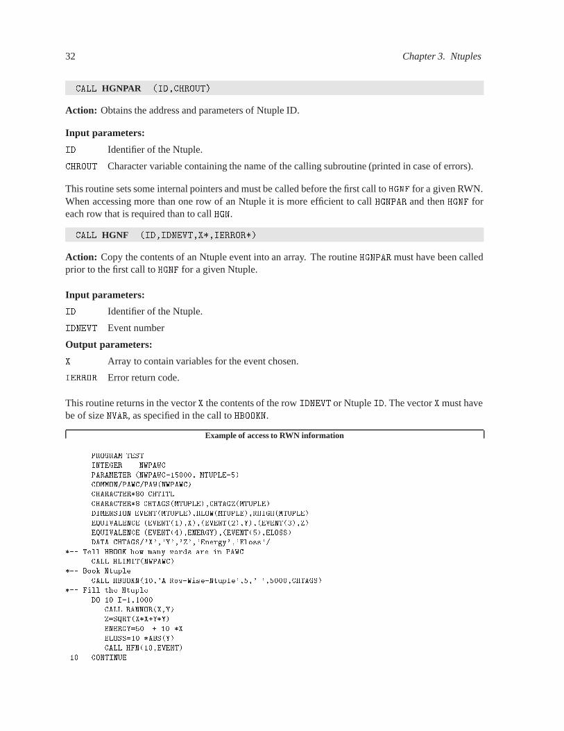
32 Chapter 3. Ntuples
CALL HGNPAR �ID�CHROUT�
Action: Obtains the address and parameters of Ntuple ID.
Input parameters:
ID Identifier of the Ntuple.
CHROUT Character variable containing the name of the calling subroutine (printed in case of errors).
This routine sets some internal pointers and must be called before the first call to HGNF for a given RWN.When accessing more than one row of an Ntuple it is more efficient to call HGNPAR and then HGNF foreach row that is required than to call HGN.
CALL HGNF �ID�IDNEVT�X��IERROR��
Action: Copy the contents of an Ntuple event into an array. The routine HGNPAR must have been calledprior to the first call to HGNF for a given Ntuple.
Input parameters:
ID Identifier of the Ntuple.
IDNEVT Event number
Output parameters:
X Array to contain variables for the event chosen.
IERROR Error return code.
This routine returns in the vector X the contents of the row IDNEVT or Ntuple ID. The vector X must havebe of size NVAR, as specified in the call to HBOOKN.
Example of access to RWN information
PROGRAM TESTINTEGER NWPAWC
PARAMETER �NWPAWC������ MTUPLE���COMMON�PAWC�PAW�NWPAWC�CHARACTER �� CHTITL
CHARACTER � CHTAGS�MTUPLE�CHTAGZ�MTUPLE�DIMENSION EVENT�MTUPLE�RLOW�MTUPLE�RHIGH�MTUPLE�
EQUIVALENCE �EVENT���X��EVENT���Y��EVENT��Z�EQUIVALENCE �EVENT���ENERGY��EVENT���ELOSS�DATA CHTAGS��X��Y��Z��Energy��Eloss��
�� Tell HBOOK how many words are in PAWC�CALL HLIMIT�NWPAWC�
�� Book Ntuple
CALL HBOOKN����A Row�Wise�Ntuple��� �����CHTAGS� �� Fill the Ntuple
DO �� I������CALL RANNOR�XY�Z�SQRT�X X�Y Y�
ENERGY���� � ��� XELOSS���� ABS�Y�CALL HFN���EVENT�
�� CONTINUE

3.5. Get information about an Ntuple 33
�� Obtain the definitions of the Ntuple
NVAR � MTUPLECALL HGIVEN���CHTITLNVARCHTAGZRLOWRHIGH�PRINT �Definitions of Ntuple � ���
PRINT � Title� �CHTITL���LENOCC�CHTITL��PRINT � Number of variables� �NVAR
DO �� I��NVARPRINT ����IRLOW�I�RHIGH�I�
���� FORMAT�� Min�Max values for column � �I�XF����
� �XF������� CONTINUE
�� Get the contents of �event� �
CALL HGNPAR����TEST��CALL HGNF���EVENTIERR�
PRINT IERREVENT �� Get the number of events in this Ntuple
CALL HNOENT���NEVENT�
PRINT NEVENT�� CONTINUE
END
3.5.2 Retrieve the contents of a CWN into a common block
CALL HGNT �ID�IDNEVT�IERR��
Action:
Retrieve information about a CWN row.
Input parameters:
ID Identifier of the Ntuple.
IDNEVT Number of the event about which information is required.
Output parameter:
IERR Error return code (�� if event was found)
The information is restored at the addresses specified by HBNAME or HBNAMC (for CHARACTER data). Ifthe information is being retrieved by a program other than the one that wrote the Ntuple then HBNAME orHBNAMC must be called as appropriate (see below).
CALL HBNAME�ID� ����CLEAR��
CALL HBNAME�IDCHBLOKVARIABLE��SET��
These calls are required as HBOOK must obtain the location at which the requested information is to bereturned which is obviously not valid between programs. The first call clears all the addresses stored byHBOOK for the specified Ntuple and the second one sets the addresses for the variables in block CHBLOK
starting at variable VARIABLE. The second call should be repeated for every block of which data has tobe retrieved. The routine HUWFUN will generate these calls automatically in the skeleton user function.

34 Chapter 3. Ntuples
CALL HGNTB �ID�CHBLOK�IROW�IERR��
Action:
Retrieve information about a named block in an Ntuple row.
Input parameters:
ID Identifier of the Ntuple.
CHBLOK Character variable specifying the block that is to be retrieved.
IROW Number of the row about which information is required.
Output parameter:
IERR Error return code (�� if row was found)
The information is restored at the addresses specified by HBNAME or HBNAMC (for CHARACTER data).
CALL HGNTV �ID�CHVAR�NVAR�IROW�IERR��
Action:
Retrieve information about the named variables in an Ntuple row.
Input parameters:
ID Identifier of the Ntuple.
CHVAR Array of character variables specifying the variables that are to be retrieved.
NVAR Number of character variables specified in CHVAR.
IROW Number of the row about which information is required.
Output parameter:
IERR Error return code (�� if row was found)
The information is restored at the addresses specified by HBNAME or HBNAMC (for CHARACTER data).
You should only call HBNAME for the blocks that contain variables you want to read using HGNTV. If youcall HBNAME for all blocks you should have a PAWC which is at least the same size as the one you used tocreate the Ntuple. If not you will run out of memory.
Also changing the buffer size will not help because the buffer used for reading will be the same size asthe buffer used to write the Ntuple.
There is a special option in HBNAME with which you can tell HBNAME to only set the address for a singlevariable in a block (this option is used by PAW to reduce memory usage).
To set the address for a single variable call HBNAME (or HBNAMC) as follows:
CALL HBNAME�ID BLOCK IADDR ��SET�NTVAR��
This will tell HGNTV to restore the Ntuple variable NTVAR in address IADDR. Using this form of HBNAMEwill only reserve buffer space for the variables you plan to read and not for all variables in the block.However, you have to be careful that when you change the list of variable for HGNTV to also add or removethe correct HBNAME calls.

3.5. Get information about an Ntuple 35
CALL HGNTF �ID�IROW�IERR��
Action:Retrieve information about all variables specified in a previous call to either HGNT, HGNTB or HGNTV, inan Ntuple row. This routine is much faster than either HGNT, HGNTB or HGNTV.
Input parameters:
ID Identifier of the Ntuple.
IROW Number of the row about which information is required.
Output parameter:
IERR Error return code (�� if row was found)
The information is restored at the addresses specified by HBNAME or HBNAMC (for CHARACTER data).
CALL HNTVDEF �ID��IVAR�CHTAG�BLOCK�ITYPE�
Action:Returns the definition as given in HBNAME for the variable with index IVAR in Ntuple ID�. The Ntuplemust already be in memory.
3.5.3 Generate a user function
HBOOK can automatically produce a skeleton user selection function, which includes the Ntuple decla-ration via the calls HBNT, HBNAME and HBNAMC, and can be used in a later run to access the elements of theNtuple. Two cases are available; one for use in batch and the other for use with paw. In the first case thecommon block names will be those specifed by the user in the call to HBNAME or HBNAMC. For paw, thesecommon names are �PAWCR��, �PAWCR�� and �PAWCCH� for storing the “single precision” (LOGICAL,INTEGER and REAL��), “double precision” (REAL�� and COMPLEX) and CHARACTER data respectively.
CALL HUWFUN �LUN�ID�CHFUN�ITRUNC�CHOPT�
Action:Write an user function or subroutine to access an Ntuple.
Input parameters:
LUN Logical unit used to write the user routine. LUN must be opened before this call.
ID Identifier of the Ntuple.
CHFUN Character variable specifying the routine name.
ITRUNC All variable names will be truncated to ITRUNC characters. ITRUNC�� is no truncation.
CHOPT Character variable specifying the desired options.
�B� Make an user subroutine for batch usage (i.e. with HBNAME and HBNAMC calls) (default).�P� Make a paw selection function.
A simple example of the two kinds of skeletons generated with routine HUWFUN is given below. Anothermore complex example can be found on page 47, where the code of a fully worked out subroutine basedon such a sketeton can also be studied.In paw, the command UWFUNC generates a skeleton for the RWN or CWN analysis function automatically.
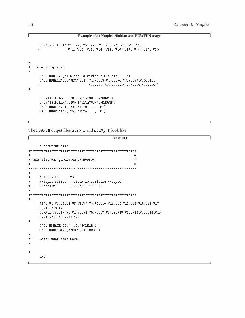
36 Chapter 3. Ntuples
Example of an Ntuple definition and HUWFUN usage
COMMON �CVECT� V� V� V V� V� V� V� V� V� V��
� V�� V�� V� V�� V�� V�� V�� V�� V�� V��
���
���
�� book N�tuple ��
CALL HBNT����� block �� variable N�tuple� � ��
CALL HBNAME����VECT�V��V�V�VV�V�V�V�V�V�V��V��
� V��V�V��V��V��V��V��V��V����
���
OPEN���FILE��nt���f�STATUS��UNKNOWN��
OPEN���FILE��nt��p�f�STATUS��UNKNOWN��
CALL HUWFUN��� �� �NT��� � �B��
CALL HUWFUN��� �� �NT��� � �P��
���
The HUWFUN output files nt���f and nt��p�f look like:
File nt20.f
SUBROUTINE NT��
This file was generated by HUWFUN�
N�tuple Id� ��
N�tuple Title� � block �� variable N�tuple
Creation� �������� ��������
REAL V�V�VV�V�V�V�V�V�V��V��V��V�V��V��V��V��
� V��V��V��
COMMON �VECT� V�V�VV�V�V�V�V�V�V��V��V��V�V��V��
� V��V��V��V��V��
CALL HBNAME���� ����CLEAR��
CALL HBNAME����VECT�V���SET��
�� Enter user code here
END

3.5. Get information about an Ntuple 37
File nt20p.f
REAL FUNCTION NT����
This file was generated by HUWFUN�
N�tuple Id� ��
N�tuple Title� � block �� variable N�tuple
Creation� �������� ��������
COMMON �PAWIDN� IDNEVTVIDN�VIDN�VIDNVIDN����
REAL V�V�VV�V�V�V�V�V�V��V��V��V�V��V��V��V��
� V��V��V��
COMMON �PAWCR�� V�V�VV�V�V�V�V�V�V��V��V��V�V��
� V��V��V��V��V��V��
�� Enter user code here
NT�� � ��
END
3.5.4 Optimizing event loops
paw is able, before starting the loop over the events, to find out which are the columns of the CWN whichare actually referenced in any given query (command line selection expression or COMIS routine). Onlythe columns which are referenced will be read from the file.
If you analyse Ntuple data without paw, it is your own responsibility to find out and specify which are thecolumns referenced via the routines HGNTV or HGNTB (if all variables in a block are needed).
This optimization can be very important. Assume, for instance, that a 100 Mbyte file contains an Ntupleconsisting of 300 columns, and that 3 columns are referenced. Then without optimization the complete100 Mbyte file will have to be read, while, by specifying the columns used, only 1 Mbyte will be input.

38 Chapter 3. Ntuples
3.6 Ntuple operations
Duplicate Ntuples
CALL HNTDUP �ID��ID��NEWBUF�CHTITL�CHOPT�
Action: Duplicate the definition of an Ntuple into a new Ntuple with the same definitions as the originalone, but with 0 entries.
Input parameters:
ID� Identifier of original Ntuple
ID� Identifier of new Ntuple
NEWBUF Buffer size
NEWBUF�� use buffer size of ID�
NEWBUF�� use current buffer size(10000 for RWN’s)
NEWBUF�� use actually specified value as buffer size
CHTITL Character variable specifying the the new title for the duplicate Ntuple. If CHTITL�� � use theoriginal title.
CHOPT Character variable specifying the desired option
CHOPT�� � use original value (disk or memory resident)
CHOPT��M� make the Ntuple memory resident
CHOPT��A� interactive mode: sets the addresses to �PAWCR��.
Rename a column in an Ntuple
CALL HRENAME �ID��CHOLD�CHNEW�
Action: Renames a column in an Ntuple. CHOLD of ntuple ID into CHNEW. Duplicate the definitionof an Ntuple into a new Ntuple with the same definitions as the original one, but with 0 entries.
Input parameters:
ID� Identifier of Ntuple
CHOLD Character variable with old column name
CHNEW Character variable with new column name
One-dimensional convolution of Ntuple
CALL HCONVOL �ID��ID��ID��IERROR��
Action: Perform a one-dimensional convolution of the Ntuple with respect to an other�. All histogramsmust pre-exist prior to calling this routine.
�Original code written by Per Steinar Iversen (PerSteinar�Iversen fi�uib�no).

3.6. Ntuple operations 39
Input parameters:
ID� Ntuple identifier (this Ntuple can be 1-D or 2-D). It is used as kernel for the convolution ofID�.
ID� Ntuple to be convoluted
ID� Ntuple resulting from the convolution of ID� with ID�
Output parameters:
IERROR error return code.
Discussion
This method scales badly for large histograms. The best general algorithm would be to unpack the his-tograms, add a suitable number of zeros, do the two FFTs, multiply the transforms, do yet another FFTand stuff the resulting histogram back into HBOOK. However, for small histograms, the naive methodis probably faster, especially if recoded in terms of lower level calls. It will also work with 1-D and 2-Dkernel-histograms that do not have matched coordinate systems - the FFT method implies equal binsizein X and Y for the kernel and the histogram to be folded. This simple method uses HBOOK to avoid thisin one (X) dimension at least, corresponding to folding in a constant resolution term.
Example of use
CALL HBOOK����Kernel � � �D���������������
CALL HBOOK����Kernel � � �D��������������������������
CALL HBPRO������
CALL HBOOK���Kernel � �D��������������������������
CALL HBPRO�����
CALL HBOOK����Function����������������
CALL HBOOK����Result �������������������
CALL HBOOK����Result �������������������
CALL HBOOK����Result ������������������
DO �� I��������
CALL RANNOR�AB�
CALL HFILL��A�������
CALL HFILL��B�������
CALL RANNOR�AB�
CALL HFILL��A����� RNDM�I�����
CALL HFILL��B����� RNDM�I�����
CALL RANNOR�AB�
CALL HFILL�A����� SQRT�RNDM�I��������
CALL HFILL�B����� SQRT�RNDM�I��������
X � ��� �RNDM�I�����������
CALL HFILL��X�������
�� CONTINUE
CALL HCONVOL����IERROR�
CALL HCONVOL����IERROR�
CALL HCONVOL���IERROR�

40 Chapter 3. Ntuples
3.7 Ntuple examples
The first example shows the use of Row-Wise-Ntuples, containing only floating point data.
Creating and using a RWN
SUBROUTINE HEXAM�
������������
� Example of N�tuples�
������������
DIMENSION X��
CHARACTER � CHTAGS��
DATA CHTAGS�� X �� Y �� Z ��
��������������������������������������������
�
Reopen data base
CALL HROPEN���HEXAM���hexam�dat��U�����ISTAT�
CALL HBOOK�����TEST�����������
CALL HBOOK�����TEST�����������������
CALL HBOOKN���N�TUPLE����HEXAM�����CHTAGS�
DO �� I�������
CALL RANNOR�AB�
X����A
X����B
X���A A�B B
CALL HFN��X�
�� CONTINUE
CALL HROUT��ICYCLE� ��
CALL HPROJ����������������
CALL HPROJ�����������������
CALL HPRINT���
CALL HROUT���ICYCLE� ��
CALL HROUT���ICYCLE� ��
CALL HLDIR�� �� ��
CALL HREND��HEXAM���
CLOSE ���
END

3.7. Ntuple examples 41
Output Generated
TEST�
HBOOK ID � � DATE �������� NO � �
� �� I I I�� I I I II�� II I II I �� I II II� I I�� I I�� III I�� I I�� I I� I I�� I I �� I II �� I II �� II II� I I� I I� I I � I II � II II I I � II II� I I� III I� II I
CHANNELS � �� � � � � � � � � � ���� �������� �������� �������� �������� �������� �������� �������� �������� �������� ����
CONTENTS � ���������������������������������������������� � ��������������� ��������������������������������������������� ������������������ � ������������� ����� ������������������ ���� ��������� �������������������� ���� ���� ����
LOWEDGE �� ���������������������������������� ��������������������������������� ������ �������������� ������������� �������������� ������������� �������������� ������ ��������������������������������������������������������������������������������
� ENTRIES � � � ALL CHANNELS � �����E�� � UNDERFLOW � ��E�� � OVERFLOW � ���E��� BIN WID � ��E� � MEAN VALUE ������E� � R � M � S � �����E�
�

42 Chapter 3. Ntuples
TEST�
HBOOK ID � �� DATE �������� NO � ��
CHANNELS �� U � � � O
� N �� ��������� ������� V
����������������������������
OVE � ���� � � � OVE
�� � � ��� � �� �� � � ��
�� � � � �� � ��� � � � ��
�� � ������EBCB����� � � � ��
�� � �� ��B�HJIIKC������ � ��
�� � � � ���CTJY�WQWUF����� � ��
�� � ���BRX������WMF�� � � ��
� � � ��DS����������KC�� � ��
� � � ���IY����������RGA�� � � �
� ��LU����������VI�� � � ��
� � � ARX����������TPC� � � ��
� � � IQZ����������UFB� � ��
� � � ���PY����������SIB� � � �
� � ��JS����������QKE�� � �
�� � � � ��MT��������NN�� � � �
�� � � AIS�������QFF���� � �
�� � ��ADKQZYX�YPG����� � �
�� � �� �BELLKCNE�F����� � �
�� � � �� �����C��� ���� �
�� � � � ��� ���� � �
� � ���� ���� � �
UND � ��� ����� � � UND
����������������������������
LOWEDGE
� ������ ������
� ��������� � ��������
� I �� I
� ENTRIES � ����� PLOT II
� SATURATION AT� ��� �� I ���� I ��
� SCALE ����� ��� A�B� STATISTICS II
� STEP � ��� � MINIMUM����� I �� I
��������������������������������������������������������
� NTUPLE ID� � ENTRIES� ����� NTUPLE
��������������������������������������������������������
� Var numb � Name � Lower � Upper �
��������������������������������������������������������
� � � X � �����E��� � � ��� �E��� �
� � � Y � �����E��� � � �����E��� �
� � Z � �������E� � �������E��� �
��������������������������������������������������������
���� Directory �
� �N� NTUPLE
�� ��� TEST�
�� ��� TEST�
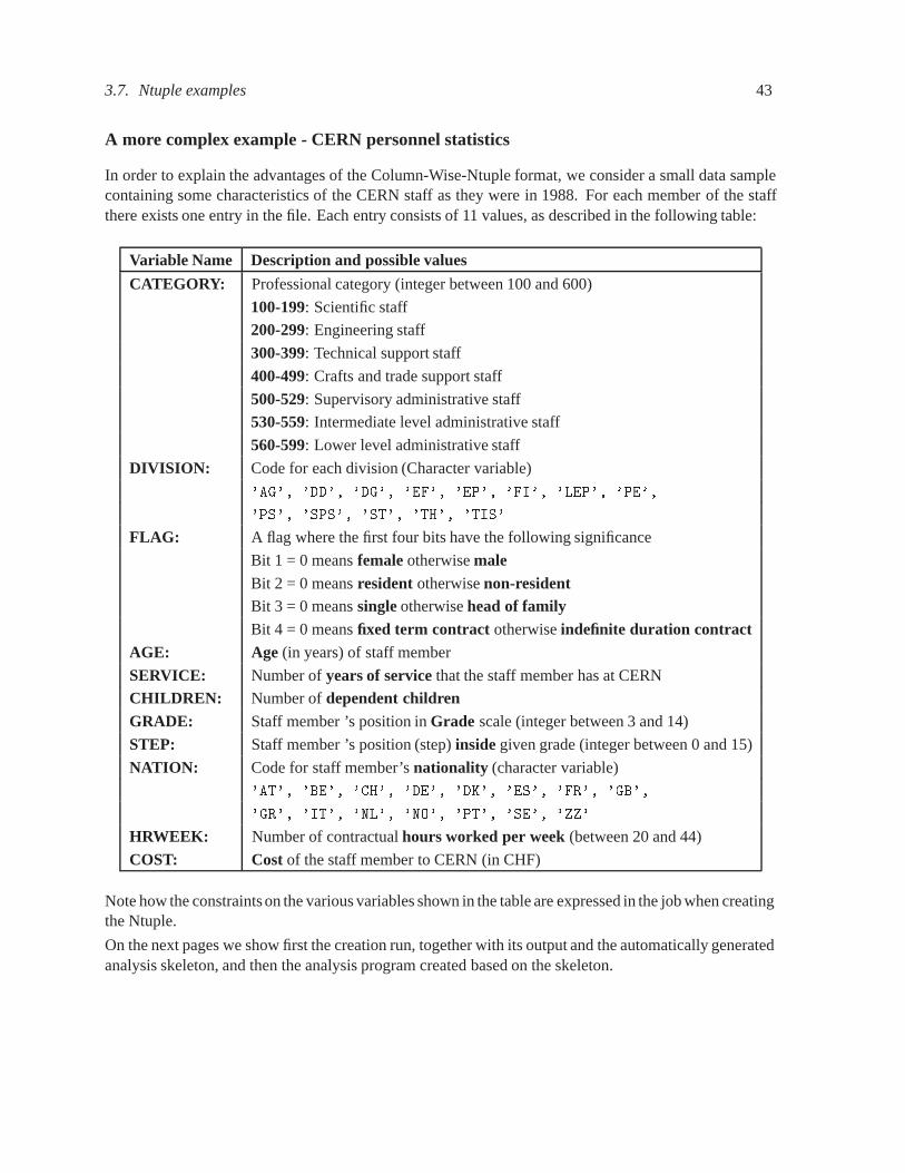
3.7. Ntuple examples 43
A more complex example - CERN personnel statistics
In order to explain the advantages of the Column-Wise-Ntuple format, we consider a small data samplecontaining some characteristics of the CERN staff as they were in 1988. For each member of the staffthere exists one entry in the file. Each entry consists of 11 values, as described in the following table:
Variable Name Description and possible values
CATEGORY: Professional category (integer between 100 and 600)
100-199: Scientific staff
200-299: Engineering staff
300-399: Technical support staff
400-499: Crafts and trade support staff
500-529: Supervisory administrative staff
530-559: Intermediate level administrative staff
560-599: Lower level administrative staff
DIVISION: Code for each division (Character variable)
�AG�� �DD�� �DG�� �EF�� �EP�� �FI�� �LEP�� �PE��
�PS�� �SPS�� �ST�� �TH�� �TIS�
FLAG: A flag where the first four bits have the following significance
Bit 1 = 0 means female otherwise maleBit 2 = 0 means resident otherwise non-residentBit 3 = 0 means single otherwise head of familyBit 4 = 0 means fixed term contract otherwise indefinite duration contract
AGE: Age (in years) of staff member
SERVICE: Number of years of service that the staff member has at CERN
CHILDREN: Number of dependent childrenGRADE: Staff member ’s position in Grade scale (integer between 3 and 14)
STEP: Staff member ’s position (step) inside given grade (integer between 0 and 15)
NATION: Code for staff member’s nationality (character variable)
�AT�� �BE�� �CH�� �DE�� �DK�� �ES�� �FR�� �GB��
�GR�� �IT�� �NL�� �NO�� �PT�� �SE�� �ZZ�
HRWEEK: Number of contractual hours worked per week (between 20 and 44)
COST: Cost of the staff member to CERN (in CHF)
Note how the constraints on the various variables shown in the table are expressed in the job when creatingthe Ntuple.
On the next pages we show first the creation run, together with its output and the automatically generatedanalysis skeleton, and then the analysis program created based on the skeleton.

44 Chapter 3. Ntuples
Creating the Ntuple
PROGRAM CERN
PARAMETER �NWPAWC � �����
PARAMETER �LRECL � �����
COMMON �PAWC� IPAW�NWPAWC�
REAL RDATA����
INTEGER CATEGORY FLAG AGE SERVICE CHILDREN GRADE STEP
� HRWEEK COST
CHARACTER � DIVISION NATION
COMMON �CERN� CATEGORY FLAG AGE SERVICE CHILDREN GRADE
� STEP HRWEEK COST
COMMON �CERNC� DIVISION NATION
CHARACTER � DIVS��� NATS����
DATA DIVS ��AG� �DD� �DG� �EF� �EP� �FI� �LEP� �PE�
� �PS� �SPS� �ST� �TH� �TIS��
DATA NATS ��AT� �BE� �CH� �DE� �DK� �ES� �FR� �GB�
� �GR� �IT� �NL� �NO� �PT� �SE� �ZZ��
CALL HLIMIT�NWPAWC�
�� open a new RZ file
CALL HROPEN���MYFILE��cern�hbook��N�LRECLISTAT�
�� book Ntuple
CALL HBNT����CERN Population�� ��
�� define Ntuple �� block with �� columns�
CALL HBNAME��� �CERN� CATEGORY �CATEGORY���������I
� FLAG�U�� AGE�������I SERVICE������I
� CHILDREN������I GRADE�����I STEP������I
� HRWEEK�������I COST�I��
CALL HBNAMC��� �CERN� DIVISION �DIVISION�C NATION�C��
�� open data file with staff information
OPEN��FILE��aptuple�dat� STATUS��OLD��

3.7. Ntuple examples 45
�� read data and store in Ntuple
�� READ�� ����F��� F����� END���� RDATA
CATEGORY � RDATA���
DIVISION � DIVS�INT�RDATA�����
FLAG � RDATA��
AGE � RDATA���
SERVICE � RDATA���
CHILDREN � RDATA���
GRADE � RDATA���
STEP � RDATA���
NATION � NATS�INT�RDATA�����
HRWEEK � RDATA����
COST � RDATA����
CALL HFNT����
GOTO ��
�� read data of person ����
�� I � ���
CALL HGNT��� I IER�
IF �IER �NE� �� THEN
PRINT �Error reading row �I
ENDIF
PRINT �Person ����� �CATEGORY� �DIVISION� �AGE� �NATION
�� print Ntuple definition
CALL HPRNT����
�� write batch version of analysis routine to file staff�f
OPEN� FILE��staff�f� STATUS��UNKNOWN��
CALL HUWFUN� �� �STAFF� � �B��
�� write Ntuple buffer to disk and close RZ file
CALL HROUT��� ICYCLE � ��
CALL HREND��MYFILE��
END
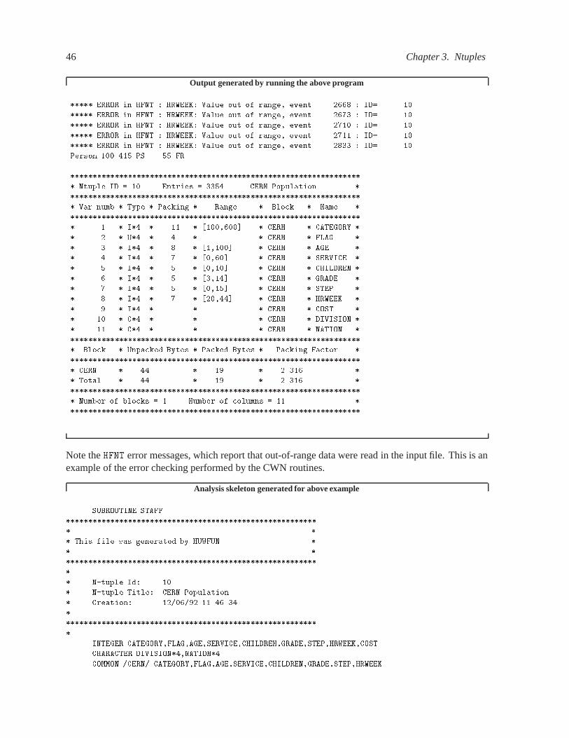
46 Chapter 3. Ntuples
Output generated by running the above program
ERROR in HFNT � HRWEEK� Value out of range event ���� � ID� ��
ERROR in HFNT � HRWEEK� Value out of range event ��� � ID� ��
ERROR in HFNT � HRWEEK� Value out of range event ���� � ID� ��
ERROR in HFNT � HRWEEK� Value out of range event ���� � ID� ��
ERROR in HFNT � HRWEEK� Value out of range event �� � ID� ��
Person ��� ��� PS �� FR
Ntuple ID � �� Entries � �� CERN Population
Var numb Type Packing Range Block Name
� I � �� �������� CERN CATEGORY
� U � � CERN FLAG
I � � ������ CERN AGE
� I � � ����� CERN SERVICE
� I � � ����� CERN CHILDREN
� I � � ���� CERN GRADE
� I � � ����� CERN STEP
� I � � ������ CERN HRWEEK
� I � CERN COST
�� C � CERN DIVISION
�� C � CERN NATION
Block Unpacked Bytes Packed Bytes Packing Factor
CERN �� �� ����
Total �� �� ����
Number of blocks � � Number of columns � ��
Note the HFNT error messages, which report that out-of-range data were read in the input file. This is anexample of the error checking performed by the CWN routines.
Analysis skeleton generated for above example
SUBROUTINE STAFF
This file was generated by HUWFUN�
N�tuple Id� ��
N�tuple Title� CERN Population
Creation� �������� �������
INTEGER CATEGORYFLAGAGESERVICECHILDRENGRADESTEPHRWEEKCOST
CHARACTER DIVISION �NATION �
COMMON �CERN� CATEGORYFLAGAGESERVICECHILDRENGRADESTEPHRWEEK

3.7. Ntuple examples 47
� COST
COMMON �CERN�� DIVISIONNATION
CALL HBNAME���� ����CLEAR��
CALL HBNAME����CERN�CATEGORY��SET��
CALL HBNAMC����CERN�DIVISION��SET��
�� Enter user code here
END
This skeleton is used in the example below to prepare a job for analysing the Ntuple data sample.
Example of Fortran code based on skeleton
PROGRAM NEWNTUP
PARAMETER �NWPAWC � �����
PARAMETER �LRECL � �����
COMMON �PAWC� IPAW�NWPAWC�
CALL HLIMIT�NWPAWC�
CALL HROPEN���MYFILE��cern�hbook�� �LRECLISTAT�
CALL HRIN���������
CALL STAFF
CALL HREND��MYFILE��
END
SUBROUTINE STAFF
This file was generated by HUWFUN�
N�tuple Id� ��
N�tuple Title� CERN Population
Creation� �������� �������
INTEGER CATEGORYFLAGAGESERVICECHILDRENGRADESTEPHRWEEKCOST
COMMON �CERN� CATEGORYFLAGAGESERVICECHILDRENGRADESTEPHRWEEK
� COST
CHARACTER DIVISION �NATION �
COMMON �CERN�� DIVISIONNATION
CHARACTER � VAR���
CALL HBNAME���� ����CLEAR�� � Clear addresses in Ntuple
CALL HBNAME����CERN�CATEGORY��SET�� � Set addresses for variables CATEGORY���
CALL HBNAMC����CERN�DIVISION��SET�� � Set addresses for variables DIVISION���

48 Chapter 3. Ntuples
�� Enter user code here
�� book the histograms
CALL HBOOK����� �Staff Age� �� ��� ��� ���
CALL HBOOK����� �Number of years at CERN� � �� �� ���
CALL HBOOK���� �Grade vs� Step� �� � ��� �� �� ��� ���
CALL HBIGBI������
CALL HBIGBI������
�� get number of entries
CALL HNOENT��� NLOOP�
�� read only the four desired columns
VAR��� � �AGE�
VAR��� � �SERVICE�
VAR�� � �GRADE�
VAR��� � �STEP�
CALL HGNTV��� VAR � � IER�
DO �� I � � NLOOP
IF �I�NE��� CALL HGNTF��� I IER�
IF �IER �NE� �� THEN
PRINT �Error reading row � I
ENDIF
CALL HFILL���� FLOAT�AGE� �� ���
CALL HFILL���� FLOAT�SERVICE� �� ���
CALL HFILL��� FLOAT�GRADE� FLOAT�STEP� ���
�� CONTINUE
CALL HISTDO
END
The summary table about the Ntuple shown below, as obtained by running the program above on theCERN Ntuple, should be compared with the table obtained during the creation run, as shown on page 46.
Output Generated
������������������������������������������������������������������������������������������������������������������������������ �� HBOOK HBOOK CERN VERSION ���� HISTOGRAM AND PLOT INDEX ������ �� ������������������������������������������������������������������������������������������������������������������������������� �� NO TITLE ID B�C ENTRIES DIM NCHA LOWER UPPER ADDRESS LENGTH �� ������������������������������������������������������������������������������������������������������������������������������� �� �� � CERN Population � N ����� �� �� �� �� � Staff Age �� �� �� � � X � ��E�� �� E�� �� �� � �� �� �� � Number of years at CERN �� �� �� � � X � �E� �� E�� ����� �� �� �� �� � Grade vs� Step �� �� �� � � X �� ��E�� �� E�� ����� ��� �� Y �� �E� ���E�� ���� ��� �� ������������������������������������������������������������������������������������������������������������������������������
MEMORY UTILISATION
MAXIMUM TOTAL SIZE OF COMMON �PAWC� �
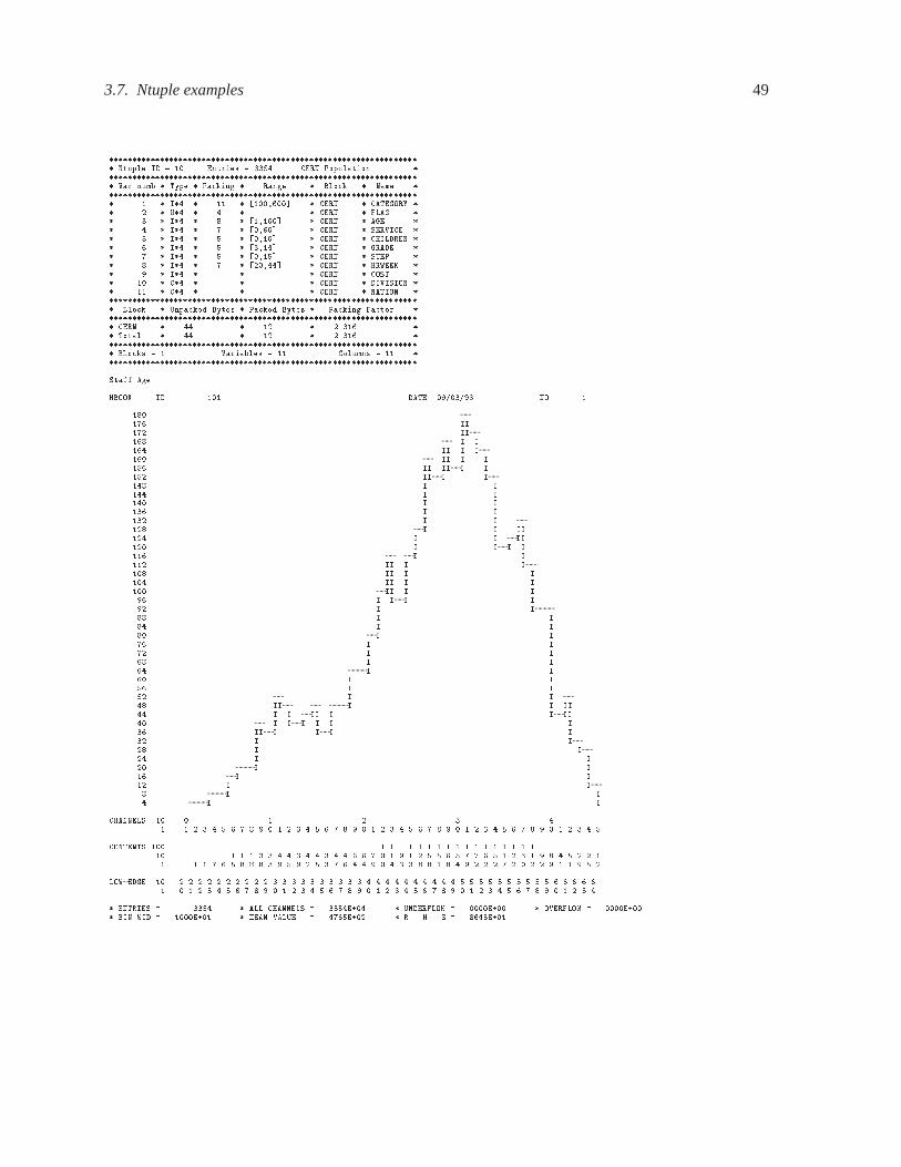
3.7. Ntuple examples 49
������������������������������������������������������������������� Ntuple ID � � Entries � �� � CERN Population �������������������������������������������������������������������� Var numb � Type � Packing � Range � Block � Name �������������������������������������������������������������������� � � I�� � �� � ����� � CERN � CATEGORY �� � � U�� � � � � CERN � FLAG �� � � I�� � � � ����� � CERN � AGE �� � � I�� � � � ���� � CERN � SERVICE �� � I�� � � ���� � CERN � CHILDREN �� � � I�� � � ������ � CERN � GRADE �� � � I�� � � ��� � � CERN � STEP �� � � I�� � � � ������ � CERN � HRWEEK �� � � I�� � � � CERN � COST �� � � C�� � � � CERN � DIVISION �� �� � C�� � � � CERN � NATION �������������������������������������������������������������������� Block � Unpacked Bytes � Packed Bytes � Packing Factor �������������������������������������������������������������������� CERN � �� � �� � ����� �� Total � �� � �� � ����� �������������������������������������������������������������������� Blocks � � Variables � �� Columns � �� �������������������������������������������������������������������
Staff Age
HBOOK ID � �� DATE ������ NO � �
�� ��� II��� II��� I I��� II I I�� II I I� � II III I� � III I��� I I��� I I�� I I��� I I��� I I ��� I I II��� I I II�� I II I��� I I��� II I I�� II I I�� II I I� II I I�� I II I�� I I�� I I�� I I� I I�� I I�� I I�� I I�� I I� I I � I I � I I �� II I I II�� I I II I III� I II I I I�� III II I�� I I�� I I�� I I� I I�� I I�� I I� I I� I I
CHANNELS � � � � �� � � � � � � � � � � � � � � � � � � � � � � � � � � � � � � � � � � � �
CONTENTS � � � � � � � � � � � � � � � � �� � � � � � � � � � � � � � � � � � � � � � � � � � � � � � � � � � ��� � � � � � � � � � � � � � � � � � � � � � � � � � � � � � � � � � � � � � �
LOWEDGE � � � � � � � � � � � � � � � � � � � � � � � � � � � � � � � � � � � ��� � � � � � � � � � � � � � � � � � � � � � � � � � � � � � � � � � � � �
� ENTRIES � �� � � ALL CHANNELS � ��� �E�� � UNDERFLOW � �E� � OVERFLOW � �E�� BIN WID � ��E�� � MEAN VALUE � ���� E�� � R � M � S � �����E��
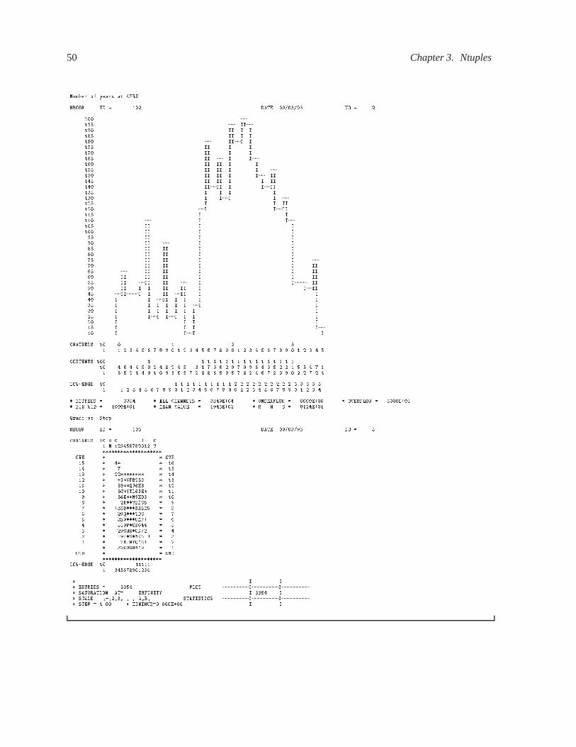
50 Chapter 3. Ntuples
Number of years at CERN
HBOOK ID � �� DATE ������ NO � �
� �� II�� II I I�� II I I�� III I�� II I I�� II I I�� II I I�� II II I I� II II I I � II II I I II�� II II I I II�� IIII I III�� I I I I�� I II I �� I I II�� I III�� I I�� I I� II I I� II I I� II I I� II I I� II II I I� II II I I� II II I I � II II I I II� II II I I II� II II II I I II II II II I I II II I I II II I III� III I II II I I� I I II I I I I� I I I I I I I I� I I I I I I I I� I II II I I I� I I I I� I I I I� I II I
CHANNELS � � � �� � � � � � � � � � � � � � � � � � � � � � � � � � � � �
CONTENTS � � � � � � � � � � � � � � � � � �� � � � � � � � � � � � � � � � � � � � � � � � � � � � ��� � � � � � � � � � � � � � � � � � � � � � � � � � � �
LOWEDGE � � � � � � � � � � � � � � � � � � � � � � � � � ��� � � � � � � � � � � � � � � � � � � � � � � � � � � � �
� ENTRIES � �� � � ALL CHANNELS � �����E�� � UNDERFLOW � �E� � OVERFLOW � � E��� BIN WID � ��E�� � MEAN VALUE � �����E�� � R � M � S � �����E��
Grade vs� Step
HBOOK ID � �� DATE ������ NO � �
CHANNELS � U � O� N ���� ������ V��������������������
OVE � � OVE� � �� � ���� � � � � �� � ���������� � ���� � �J�YFB��G � ���� � ����QJ�H� � ��� � �C�YTL�JE� � ��� � ��E��N�HD� � �� � �K��VEN� � �� � ���D���NRB� � �� � �GQ���TD� � � � �S����UM�� � �� � I�P�QKG�� � � � ���WW�QK�� � �� � ��J�S�NK � � �� � �EJMYQM�� � �
� ��A�GMNM� � �UND � � UND
��������������������LOWEDGE � �����
�� �� ��������
� I I� ENTRIES � �� � PLOT II� SATURATION AT� INFINITY I �� � I� SCALE ������������ A�B� STATISTICS II� STEP � �� � MINIMUM��E� I I

Chapter 4: Advanced features for booking and editing operations
4.1 Overview of booking options
4.1.1 Histograms with non-equidistant bins
CALL HBOOKB �ID�CHTITL�NCX�XBINS�VMX�
Action: As HBOOK�, but instead of giving the lower and upper limits, an array XBINS of NCX�� elementsis provided.
XBINS��� contains the lower edge of the first bin.
XBINS��� contains the lower edge of the second bin.
��� and so on.
XBINS�NCX��� contains the upper edge of the last bin.
4.1.2 Profile histograms
CALL HBPROF �ID�CHTITL�NCX�XLOW�XUP�YMIN�YMAX�CHOPT�
Action: Create a profile histogram. Profile histograms are used to display the mean value of Y and itsRMS for each bin in X. Profile histograms are in many cases an elegant replacement of two-dimensionalhistograms : the inter-relation of two measured quantities X and Y can always be visualized by a two-dimensional histogram or scatter-plot; its representation on the line-printer is not particularly satisfactory,except for sparse data. If Y is an unknown (but single-valued) approximate function of X , this functionis displayed by a profile histogram with much better precision than by a scatter-plot.
The following formulae show the cumulated contents (capital letters) and the values displayed by theprinting or plotting routines (small letters) of the elements for bin J.
H�J� �PY E�J� �
PY �
l�J� �Pl L�J� �
Pl
h�J� � H�J��L�J� s�J� �pE�J��L�J�� h�J� � ��
e�J� � s�J��pL�J�
The first five parameters are similar to HBOOK�. Only the values of Y between YMIN and YMAX will beconsidered. To fill a profile histogram, one must use CALL HFILL �ID�X�Y����.
H�J� is printed as the channel contents. The errors displayed are s�J� if CHOPT��S� (spread option), ore�J� if CHOPT�� � (error on mean).
Profile histograms can be filled with weights.
The computation of the errors and the text below is based on a proposal by Stephane Coutu�.
If a bin has N data points all with the same value Y (especially possible when dealing with integers), thespread in Y for that bin is zero, and the uncertainty assigned is also zero, and the bin is ignored in makingsubsequent fits. This is a problem. If
pY was the correct error in the case above, then
pY�pN would be
�Stephane Coutu, coutu roo�physics�lsa�umich�edu
51
52 Chapter 4. Advanced features for booking and editing operations
the correct error here. In fact, any bin with non-zero number of entries N but with zero spread should havean uncertainty
pY�pN.
Yet, ispY�pN really the correct uncertainty? Probably it is only true in the case where the variable Y
is some sort of counting statistics, following a Poisson distribution. This should probably correspond tothe default case. However, Y can be any variable from an original Nntuple, not necessarily distributedaccording to a Poisson distribution. Therefore several settings for the option variable CHOPT are possibleto determine how errors should be calculated (S stands for the spread in the formulae below):
� � (Default)Errors are S�
pN for S �� ��,
” ”pY�pN for S � �� N � �,
” ” �� for N � �.
�S�
Errors are S for S �� ��,
” ”pY for S � �� N � �,
” ” �� for N � �.
�I�
Errors are S�pN for S �� ��,
” ” ���p���N for S � �� N � �,
” ” �� for N � �.
The third case above corresponds to integer Y values for which the uncertainty is����, with the assump-tion that the probability that Y takes any value between Y���� and Y���� is uniform (the same argumentgoes for Y uniformly distributed between Y and Y � �); this could be useful, for instance, for the casewhere Y are ADC measurements.
4.1.3 Rounding
CALL HBINSZ ��YES���NO��
Action: Round the bin size for bookings of subsequent histograms to a reasonable value, i.e.:���������������� times an integer power of 10. HBINSZ controls a switch that, when on, roundsthe binsize, still respecting the number of bins. The switch is initially off.
Input parameters:
�YES� enable the ’reasonable rounding’ feature.
�NO� disable the ’reasonable rounding’ feature.
4.1.4 Projections, Slices, Bands
CALL HBPRO �ID�VMX�
Action: Books the projections of a 2-dimensional histogram as two 1-dimensional histograms.
Input parameters:

4.1. Overview of booking options 53
ID identifier of an existing 2-dimensional histogramID�� means book projections for all existing 2-dimensional histograms.
VMX upper limit of single channel content.
Remark:
– if ID does not exist, or is a 1-dimensional histogram, the call does nothing
– see HBOOK� for details about VMX
– booking of projections can be executed only after the 2-dimensional histogram with identifier IDhas been booked.
CALL HBPROX �ID�VMX� and CALL HBPROY �ID�VMX�
Action: Books projection onto X or Y only. See HBPRO for more details.
CALL HBANDX �ID�YMI�YMA�VMX�
Action: Books a projection onto X, restricted to the Y interval (YMI�YMA).
Input parameters:
ID identifier of an existing 2-dimensional histogram
YMI lower limit of Y interval
YMA upper limit of Y interval
VMX maximum value to be stored in 1 channel.
The same remarks as for HBPRO apply.
CALL HBANDY �ID�XMI�XMA�VMX�
Action: As HBANDX but the projection is onto Y.
CALL HBSLIX �ID�NSLI�VMX�
Action: Books slices along Y of 2-dimensional histograms as NSLI 1-dimensional histograms.Each slice is a projection onto X restricted to an interval along the Y axis.
Input parameters:
ID identifier of an existing 2-dimensional histogram
NSLI number of slices
VMX maximum value to be stored in 1 channel.
The same remarks as for HBPRO apply.
CALL HBSLIY �ID�NSLI�VMX�
Action: As HBSLIX but slices are projected onto Y.
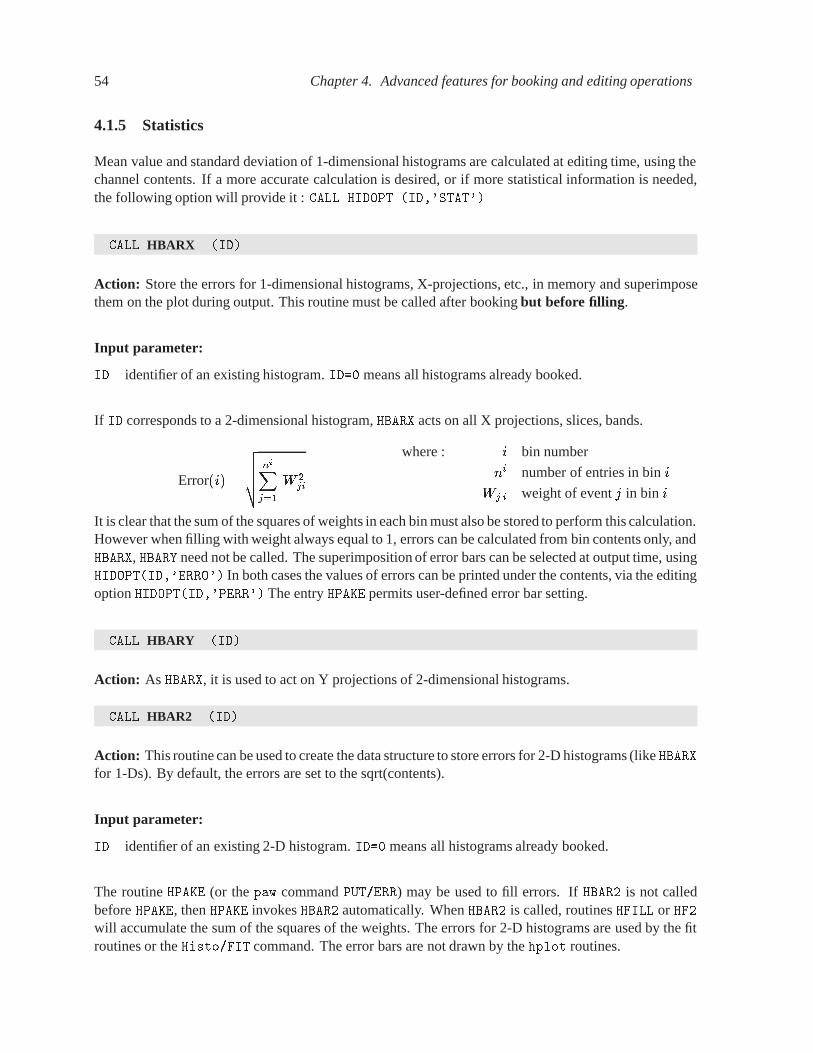
54 Chapter 4. Advanced features for booking and editing operations
4.1.5 Statistics
Mean value and standard deviation of 1-dimensional histograms are calculated at editing time, using thechannel contents. If a more accurate calculation is desired, or if more statistical information is needed,the following option will provide it : CALL HIDOPT �ID��STAT��
CALL HBARX �ID�
Action: Store the errors for 1-dimensional histograms, X-projections, etc., in memory and superimposethem on the plot during output. This routine must be called after booking but before filling.
Input parameter:
ID identifier of an existing histogram. ID�� means all histograms already booked.
If ID corresponds to a 2-dimensional histogram, HBARX acts on all X projections, slices, bands.
Error�i� �
vuuut niXj��
W �ji
where : i bin number
ni number of entries in bin i
Wj i weight of event j in bin i
It is clear that the sum of the squares of weights in each bin must also be stored to perform this calculation.However when filling with weight always equal to 1, errors can be calculated from bin contents only, andHBARX, HBARY need not be called. The superimposition of error bars can be selected at output time, usingHIDOPT�ID��ERRO�� In both cases the values of errors can be printed under the contents, via the editingoption HIDOPT�ID��PERR�� The entry HPAKE permits user-defined error bar setting.
CALL HBARY �ID�
Action: As HBARX, it is used to act on Y projections of 2-dimensional histograms.
CALL HBAR2 �ID�
Action: This routine can be used to create the data structure to store errors for 2-D histograms (like HBARXfor 1-Ds). By default, the errors are set to the sqrt(contents).
Input parameter:
ID identifier of an existing 2-D histogram. ID�� means all histograms already booked.
The routine HPAKE (or the paw command PUT�ERR) may be used to fill errors. If HBAR� is not calledbefore HPAKE, then HPAKE invokes HBAR� automatically. When HBAR� is called, routines HFILL or HF�will accumulate the sum of the squares of the weights. The errors for 2-D histograms are used by the fitroutines or the Histo�FIT command. The error bars are not drawn by the hplot routines.

4.1. Overview of booking options 55
4.1.6 Function Representation
CALL HBFUN1 �ID�CHTITL�NX�XMI�XMA�FUN�
Action: Books 1-dimensional histogram and fills it with the values of the external function FUN�X� com-puted at the centre of each bin. One computer word per channel is used.
The first five parameters are as for HBOOK�.
Input parameters:
ID histogram identifier, integer non zero
CHTITL histogram title (character variable or constant up to 80 characters)
NX number of channels
XMI lower edge of first channel
XMA upper edge of last channel
FUN real function of one variable, to be declared EXTERNAL in the calling subroutine, and to besupplied by the user.
CALL HBFUN2 �ID�CHTITL�NX�XMI�XMA�NY�YMI�YMA�FUN�
Action: Books a 2-dimensional histogram and fills it with the values of the external function FUN�X�Y�,computed at the centre of each bin. One computer word per channel is used.
The first eight parameters are as for HBOOK�.
Input parameters:
ID histogram identifier, integer
CHTITL histogram title (character variable or constant up to 80 characters)
NX number of channels in X
XMI lower edge of first X channel
XMA upper edge of last X channel
NY number of channels in Y
YMI lower edge of first Y channel
YMA upper edge of last Y channel
FUN real function of two variables, to be declared EXTERNAL in the calling subroutine, and to besupplied by the user.
CALL HFUNC �ID�FUN�
Action: Samples the functionFUN, which must have been declared EXTERNAL, at the centre of the bins of ahistogram. The function will be superimposed onto the histogram at editing time and its values optionallyprinted out (see HIDOPT�ID��PFUN��

56 Chapter 4. Advanced features for booking and editing operations
Input parameters:
ID identifier of an existing 1-dimensional histogram.ID�� signals that the function should be calculated for all existing 1-dimensional histograms.
FUN External real function, e.g. REAL FUNCTION FUN�X�.The function parameter X will be the central value of a histogram bin. The user must returnthe corresponding function at that point as a value in FUN.
Remark:
– Not existing for 2-dimensional histograms.
– Function FUN cannot contain any call to an entry of the HBOOK package.
– HFUNC can be called several times for the same histogram identifier ID. If the latter case, the valuesof the old function will be overwritten by the new one.
– The chi-squared ��, as defined below, will be printed along with the statistical information at thebottom of the histogram.
�� �nchXi��
�C�i�� F �i���Pni
j��Wji
�
with: nch number of channels of histogram
C�i� contents of channel i
F �i� value of function at centre of channel i
ni number of entries in channel ii
Wji weight of event j in channel i, i.e.
square root of contentsC�i� or
as given by HBARX/HPAKE
4.1.7 Reserve array in memory
CALL HARRAY �ID�NWORDS�LOC��
Action: Reserves an array in the memory storage area managed by HBOOK.
Input parameters:
ID identifier of the array (pseudo-histogram)
NWORDS length of the array.
Output Parameters
LOC Address minus one in the internal hbook common block �PAWC� of the 1st element of thearray, i.e.
COMMON�PAWC�NWPAW�IXPAWC�IHDIV�IXHIGZ�IXKU�FENC���LMAIN�HCV���
DIMENSION IQ����Q����LQ������
EQUIVALENCE �LQ����LMAIN���IQ����LQ�����Q����IQ����
IADDR � Q�LOC���
Remark:
At any time the address of preudo-histogram ID can be obtained with HLOCAT�ID�LOC�

4.2. Filling Operations 57
4.1.8 Axis labels and histograms
A set of routines, HLABEL, HFC� and HFC�, allows one to associate labels with histogram channels. Thisassociation can be made before or after a histogram is filled, but it has the advantage that the label infor-mation get stored in the histogram data structure, so that it is available for all future plots in an automaticway in the HPLOT and PAW packages. Printing histograms with associated alphanumeric labels is notimplemented in the line-printer oriented routines of HBOOK.
CALL HLABEL �ID�NLAB��CLAB��CHOPT�
Action: Associates alphanumeric labels with a histogram. This routine can be called for a histogram afterit has been filled, and then the labels specified will be shown on the respective axes. The routine can alsobe called before a histogram is filled , and in this case, when filling, a certain order can be imposed. Bydefault the entries will be automatically ordered.
Input parameters:
ID Histogram identifier.
NLAB Number of labels.
CHOPT Character variable specifying the option desired.
� � As �N� below.�N� Add NLAB new labels read in CLAB to histogram ID.�R� Read NLAB labels into in CLAB from histogram ID.�X� X-axis is being treated (default).
�Y� Y-axis is being treated.�Z� Z-axis is being treated.�S� Sorting order of the labels:
�S� default, as �SA�;
�SA� alphabetically;�SE� reverse alphabetical order;�SD� by increasing channel contents (after filling);�SV� by decreasing channel contents (after filling).
�T� Modify (replace) NLAB existing labels read from CLAB in histogram ID.
Input/Output parameter:
�CLAB� Character variable array with NLAB elements (input and output).
Notes:
– For one-dimensional histograms HLABEL can be called at any time.
– For two-dimensional histograms one must call HLABEL with option �N� for each axis between thecall to HBOOK� and the first call to HFC�.
4.2 Filling Operations
It is possible to speed up the filling process with the loss of some protection, and to globally transfer anarray or a matrix to a histogram.

58 Chapter 4. Advanced features for booking and editing operations
4.2.1 Fast Filling Entries
If the program that is using HBOOK fills many histograms several times a substantial fraction of time canbe spent by HFILL in searching for the histogram it has to fill, deciding which type of histogram it is andunpacking and packing bits if more than one channel is to be stored in one computer word. To reduce theoverall filling time, there are several actions that can be taken
– Bypass part of the logic that finds out the characteristicsof the histogramto fill. This can be achievedby using, instead of HFILL the special filling entries described in this section.
– Avoid packing more than one channel in a computer word.
For these reasons it is recommended to use always HFILL at the development stage, and replace it laterwith HF�, HF�, etc. only when a rather stable program is going to be used extensively.
Calls to HFILL and HF� or HF� cannot be mixed on the same ID.
CALL HF1 �ID�X�WEIGHT�
Action: Analogous to HFILL on a 1-dimensional histogram but HBARX and HIDOPT�ID��STAT�� areignored.
Input parameters:
ID histogram identifier
X value of the abscissa
WEIGHT event weight
CALL HF1E �ID�X�WEIGHT�ERRORS�
Action: Analogous to HF�, but also the errors are accumulated.
Input parameters:
ID histogram identifier.
X value of the abscissa.
WEIGHT the content is incremented by WEIGHT.
ERROR the error is incremented by ERROR���.
===¿ HF1E Fills a 1-D histogram
SUBROUTINE HF1E(ID,X,W,E)
- ID : Histogram identifier. - X : Value of the abscissa - W : Content is incremented by W - E : Errors isincremented by E**2

4.2. Filling Operations 59
CALL HF2 �ID�X�Y�WEIGHT�
Action: Analogous to HFILL on a 2-dimensional histogram except that projections, bands, slices are notfilled. HBARY is ignored as well.
Input parameters:
ID histogram identifier
X value of the abscissa
Y value of the ordinate
WEIGHT event weight
CALL HFF1 �ID��NID��X�WEIGHT�
Action: Analogous to HF� with the same restrictions. Cannot be used for variable-bin-width histograms.
Input parameters:
ID histogram identifier
NID is a histogram-specific variable that has to be provided by the user.Before the first call, NID must be initialized to 0.In subsequent calls to HFF� the constant NIDmust then be used in order to skip the calculationof the histogram address.
X value of the abscissa
WEIGHT event weight
Output parameter:
NID After the first call to HFF�, NID will contain the current address of histogram ID.
CALL HFF2 �ID��NID��X�Y�W�
Action: Analogous to HF� with the use of the parameter NID as explained for HFF�.
CALL HFPAK1 �ID�NID�V�N�
Action: Fill an histogram using the contents of a vector.
Input parameters:
ID histogram identifier
V array containing the values to be entered into the histogram.
N length (dimension) of the array V
Input/output parameter:
�NID� address of histogram (see HFF�)
This subroutine has the same effect as
DO �� I���N
�� CALL HFF��ID�NID�V�I�����
where the array V of N words must have been filled previously by the user.

60 Chapter 4. Advanced features for booking and editing operations
CALL HIPAK1 �ID�NID�IV�N�
Action: Analogous to HFPAK�, except that the user vector contains now integers instead of real numbers.
4.2.2 Global Filling
A vector or matrix can be transferred into a histogram with a single call.
CALL HPAK �ID�CONTEN�
Action: Transfer the contents of an array as channel contents into an histogram. The original contents ofthe histogram are overwritten.
Input parameters:
ID an existing histogram identifier
CONTEN a user array, suitably dimensioned
Remark:
– In the case of a 1-dimensional histogram, the dimension of the array must at least be equal to thenumber of histogram channels (NCHAN), i.e. DIMENSION CONTEN�NX� with NX�NCHAN
– In the case of a 2-dimensional histogram, the dimensions of the array must exactly be equal to thenumber of histogram channels (NCHANX and NCHANY),i.e. DIMENSION CONTEN�NX�NY� with NX�NCHAN and NY�NCHANY
Projections and slices, if present for the given histogram, are not filled.
CALL HPAKAD �ID�CONTEN�
Action: Similar to HPAK, but instead of overwriting the channel contents, the array values are added tothe respective channel contents.
CALL HPAKE �ID�ERRORS�
Action: Store the contents of an array as the errors for the bins of the 1-dimensional histogram for whichthe option HBARX has been invoked.
Input parameters:
ID histogram identifier
ERRORS user array containing the errors to be assigned to the histogram bin contents. Its dimensionshould be at least equal to the number of channels in histogram ID.
Remark:
If the HBARX option was not set for the given histogram, then it is activited by a call to HPAKE.
4.2. Filling Operations 61
4.2.3 Filling histograms using character variables
Routines for which, using routine HLABEL, alphanumeric labels were associated with the histogram chan-nels, are filled with the routinesHFC� and HFC�. These allow, on top of by bin number, to fill an histogramby specifying a alphanumeric channel identifier.
CALL HFC1 �ID�IBIN�CLAB�W�CHOPT�
Action: Fills a channel in a one-dimensional histogram.
ID One-dimensional histogram identifier.
IBIN Number of the bin to be filled (if �� �).
CLAB Character variable containing the label describing the bin (if IBIN��).
CHOPT Character variable specifying the option desired.
� � default, as �S�;
�N� filling order, i.e. the order of the labels on the plot is given by the sequence in which theyare presented in the successive calls to the routine (this method can be very time consumingsince all channels must be scanned at each call);
�S� automatic sort;
�U� if the channel does not exist then the underflow channel is incremented (by default a newchannel is created for each new label).
Remarks:
– If IBIN���, then the channel IBIN is filled; CLAB may then be undefined.
– When a label is encountered, which is not yet known, then for options �N� and �S� a new channelis added dynamically, while for option �U� the underflow channel is incremented.
– Routine HLABEL can be called before or after HFC�.
CALL HFC2 �ID�IBINX�CLABX�IBINY�CLABY�W�CHOPT�
Action: Fills for a two-dimensional histogram the channel identified by position IBINX or label CLABXand position IBINY or label CLABY with weight W.
ID Two-dimensional histogram identifier.
IBINX Number of the X-bin to be filled (if �� �).
CLABX Character variable containing the label describing the X-bin (if IBINX��).
IBINY Number of the Y-bin to be filled (if �� �).
CLABY Character variable containing the label describing the Y-bin (if IBINY��).
W Weight of the event to be entered into the histogram.
CHOPT Character variable specifying the option desired.
� � default, as �S�;

62 Chapter 4. Advanced features for booking and editing operations
�N� filling order (see HFC�;
�S� automatic sort (default)
�U� if the channel does not exist then the underflow channel is incremented (by default a newchannel is created for each new label).
Remarks:
– For efficiency reasons, routine HLABEL must be called before HFC�.
– If IBINX���, then the channel described by IBINX is filled; CLABX may then be undefined.
– If IBINY���, then the channel described by IBINY is filled; CLABY may then be undefined.
– If the channel described by IBINX or CLABX does not exist, the underflow channel is incremented.Idem for IBINY and CLABY.
The example below shows different uses of the label routines. The input data are the same as those usedfor building the Ntuple on page 43. Three histograms are booked. For the first one (��), the number ofchannels (��) is given explicitly, and a call to HLABEL declares all the labels for that histogram. Then asecond histogram (��) is booked with one pre-declared channel. In fact this latter histogram will be filledwith HFC�, in a way completely identical to histogram ��, but channels will be dynamically added as newlabels are encountered. We also create a 2-D histogram (��), where for the y-axis we again pre-declarelabels and we fill it with a call to HFC�. After the loop, where the histograms are filled, we tell HBOOKto order the labels in the second histogram (��) according to decreasing bin contents. This shows that itis not necessary, in the 1-D case, to pre-declare the labels of a histogram, but that they can be added to ahistogram “on the fly”, i.e. while filling. The sorting order can be specified after the histogram is filled. Asstated earlier, labels are only printed on graphical output devices, so that one must use HPLOT/HIGZ tosee the effect of the label routines. The calls to the HPLOT/HIGZ routines, used to generate the PostScriptpicture shown in Fig. 4.1, are described in the HIGZ/HPLOT manual.
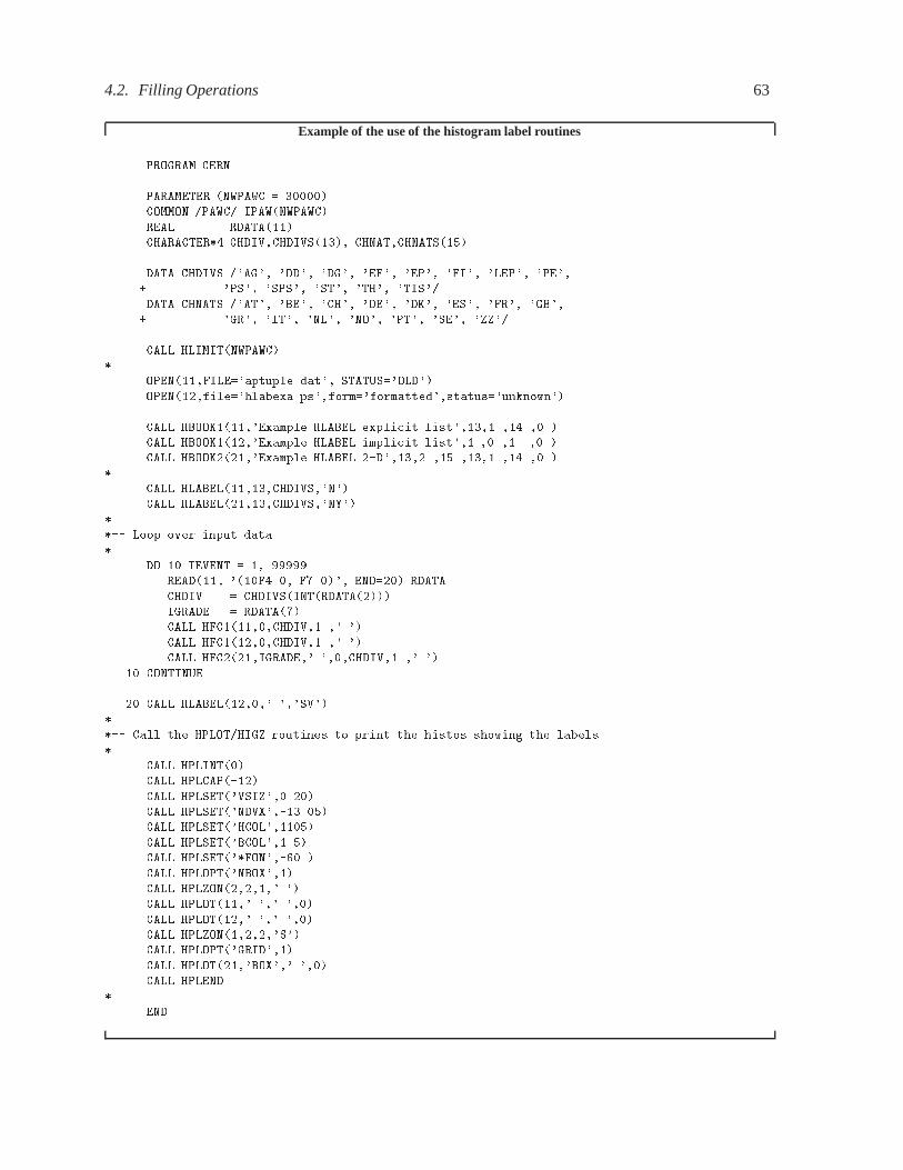
4.2. Filling Operations 63
Example of the use of the histogram label routines
PROGRAM CERN
PARAMETER �NWPAWC � �����COMMON �PAWC� IPAW�NWPAWC�
REAL RDATA����CHARACTER � CHDIVCHDIVS��� CHNATCHNATS����
DATA CHDIVS ��AG� �DD� �DG� �EF� �EP� �FI� �LEP� �PE�� �PS� �SPS� �ST� �TH� �TIS��
DATA CHNATS ��AT� �BE� �CH� �DE� �DK� �ES� �FR� �GB�� �GR� �IT� �NL� �NO� �PT� �SE� �ZZ��
CALL HLIMIT�NWPAWC�
OPEN���FILE��aptuple�dat� STATUS��OLD��
OPEN���file��hlabexa�ps�form��formatted�status��unknown��
CALL HBOOK�����Example HLABEL explicit list����������CALL HBOOK�����Example HLABEL implicit list�� ���� ���CALL HBOOK�����Example HLABEL ��D����������������
CALL HLABEL����CHDIVS�N��CALL HLABEL����CHDIVS�NY��
�� Loop over input data
DO �� IEVENT � � �����
READ��� ����F��� F����� END���� RDATA
CHDIV � CHDIVS�INT�RDATA�����IGRADE � RDATA���CALL HFC�����CHDIV��� ��
CALL HFC�����CHDIV��� ��CALL HFC����IGRADE� ��CHDIV��� ��
�� CONTINUE
�� CALL HLABEL����� ��SV��
�� Call the HPLOT�HIGZ routines to print the histos showing the labels
CALL HPLINT���CALL HPLCAP�����
CALL HPLSET��VSIZ������CALL HPLSET��NDVX�������CALL HPLSET��HCOL������
CALL HPLSET��BCOL�����CALL HPLSET�� FON������
CALL HPLOPT��NBOX���CALL HPLZON����� ��CALL HPLOT���� �� ���
CALL HPLOT���� �� ���CALL HPLZON�����S��CALL HPLOPT��GRID���
CALL HPLOT����BOX�� ���CALL HPLEND
END

64 Chapter 4. Advanced features for booking and editing operations
Example HLABEL explicit list
0
100
200
300
400
500
AG DD DG EF EP FI LEP PE PS SPS ST TH TIS
Example HLABEL implicit list
0
100
200
300
400
500
LEP PS EF SPS ST EP DD TIS AG FI PE TH DG
Example HLABEL 2-D
AG
DD
DG
EF
EP
FI
LEP
PE
PS
SPS
ST
TH
TIS
2 3 4 5 6 7 8 9 10 11 12 13 14
Figure 4.1: Example of the use of HLABEL
– The top left picture shows the contents of the histogram ordered alphabetically by label.
– The top right picture shows the same histogram, but with the bins ordered by decreasing contents,irrespective of their label.
– The lower picture shows a two-dimensional histogram, where the ordinate (Y-axis) ordered alpha-betically.
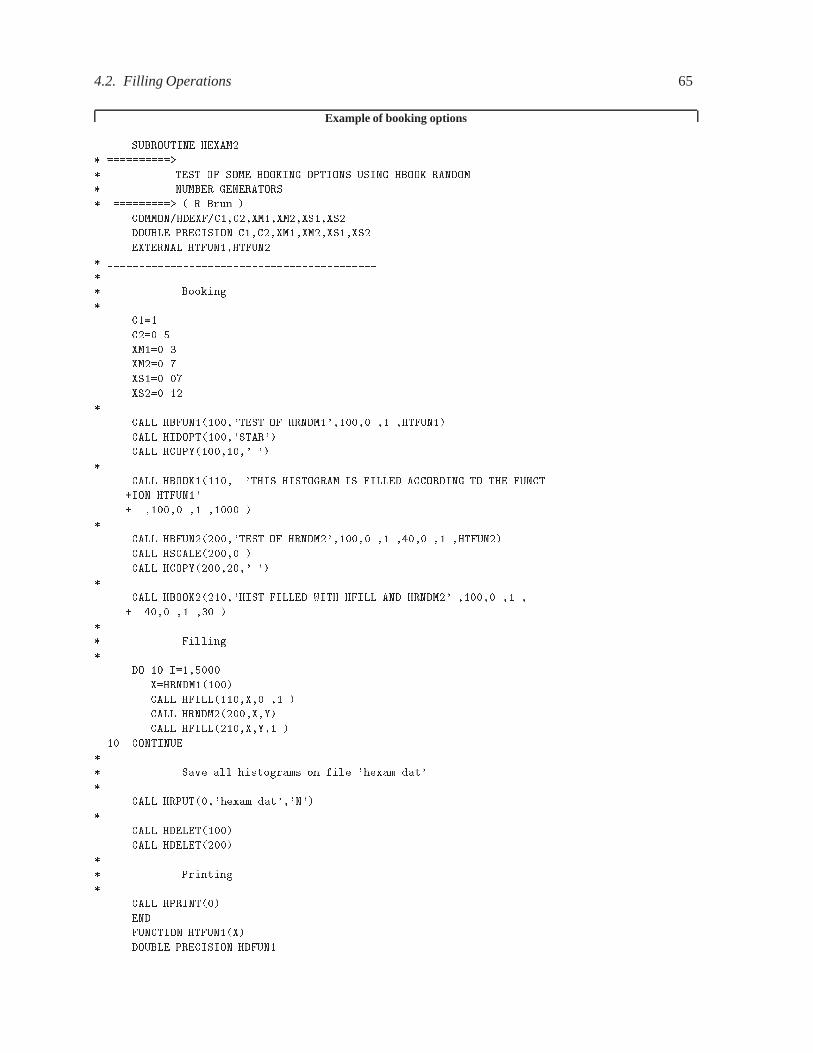
4.2. Filling Operations 65
Example of booking options
SUBROUTINE HEXAM�
������������
� TEST OF SOME BOOKING OPTIONS USING HBOOK RANDOM
� NUMBER GENERATORS�
������������ � R�Brun �
COMMON�HDEXF�C�C�XM�XM�XS�XS�
DOUBLE PRECISION C�C�XM�XM�XS�XS�
EXTERNAL HTFUN�HTFUN�
��������������������������������������������
�
Booking
C����
C�����
XM����
XM�����
XS������
XS������
CALL HBFUN������TEST OF HRNDM���������HTFUN��
CALL HIDOPT�����STAR��
CALL HCOPY������� ��
CALL HBOOK����� �THIS HISTOGRAM IS FILLED ACCORDING TO THE FUNCT
�ION HTFUN��
� �������������
CALL HBFUN������TEST OF HRNDM���������������HTFUN��
CALL HSCALE�������
CALL HCOPY������� ��
CALL HBOOK������HIST FILLED WITH HFILL AND HRNDM�� �������
� ���������
Filling
DO �� I������
X�HRNDM������
CALL HFILL����X�����
CALL HRNDM�����XY�
CALL HFILL����XY���
�� CONTINUE
Save all histograms on file �hexam�dat�
CALL HRPUT���hexam�dat��N��
CALL HDELET�����
CALL HDELET�����
Printing
CALL HPRINT���
END
FUNCTION HTFUN��X�
DOUBLE PRECISION HDFUN�

66 Chapter 4. Advanced features for booking and editing operations
HTFUN��HDFUN��X�
END
FUNCTION HTFUN��XY�
HTFUN��HTFUN��X� HTFUN��Y�
END
DOUBLE PRECISION FUNCTION HDFUN��X�
COMMON�HDEXF�C�C�XM�XM�XS�XS�
DOUBLE PRECISION C�C�XM�XM�XS�XS�A�A�X�X�
A������ ��X�XM���XS�� �
A������ ��X�XM���XS�� �
IF�A��LT������THEN
X����
ELSEIF�A��GT�����THEN
X����E�
ELSE
X��C� EXP�A��
ENDIF
IF�A��LT������THEN
X����
ELSEIF�A��GT�����THEN
X����E�
ELSE
X��C� EXP�A��
ENDIF
HDFUN��X��X�
END

4.2. Filling Operations 67
Output Generated
TEST OF HRNDM�
HBOOK ID � � DATE �������� NO � �
� ������� �� � ���� � � ���� �� ��� � ����� �� � ���� ���� � ��� ��� � � �� � � �� � � ����������� �� ���� � ���� � � �� � � ���� � ��� � � ���� � � �� � � ���� � � ��� � � ���� � � �� � �� ���� � � � ���� ������ ���� � ��� � ��� � ���� �� ����� ����������� �
CHANNELS � �� � � � � � � � � � ���� �������� �������� �������� �������� �������� �������� �������� �������� �������� ����
CONTENTS �� ������� �������������� ���������������������������������������������������������� � ������� ���� ������������ ��������������������������� ���������� ������������ ����� ����
��� ������ ��������������������������� ����������� ���������������� �������������� ������ ������������ ����� ��������������������������� ������� ���������� ����� ���������� � ������� ��������� �� ���������� ��������� �� �������� �������� ������ �� ������� ���
LOWEDGE �� ���������������������������������������� �������������������������������������������� � ���� �������� �������� �������� �������� �������� �������� �������� �������� �������� ����
� ENTRIES � � � ALL CHANNELS � �����E�� � UNDERFLOW � �E� � OVERFLOW � �E�� BIN WID � ��E� � MEAN VALUE � ����E� � R � M � S � �����E�

68 Chapter 4. Advanced features for booking and editing operations
THIS HISTOGRAM IS FILLED ACCORDING TO THE FUNCTION HTFUN�
HBOOK ID � �� DATE �������� NO �
��� ��� I��� I�� I� � II � � III��� I I��� I I�� I I��� I I��� I I��� I I��� I I�� I I��� I I��� I I�� I I�� I I� I I�� I I �� I II�� I I�� I I � I I I I I �� I I I I I I I�� I I I I I II I I �� I III I IIIIII�� I I I I I� I I I I I I � II I I II I � I I I II�� I I I I�� I I I I � I I I I I�� I I I II�� I I I I�� I I I I I �� I II I I I I I� I I IIII II I �� I II II�� I I� I I� II I
CHANNELS � �� � � � � � � � � � ���� �������� �������� �������� �������� �������� �������� �������� �������� �������� ����
CONTENTS � �������������� ������� ����� � �������� ��������������� ��� ���������������� ���������������� ��������������������������� �� ��� ���������� ����� ������ ���� ������������ ��� ����� ��
LOWEDGE �� ���������������������������������������� �������������������������������������������� � ���� �������� �������� �������� �������� �������� �������� �������� �������� �������� ����
� ENTRIES � � ALL CHANNELS � � E�� � UNDERFLOW � �E� � OVERFLOW � �E�� BIN WID � ��E� � MEAN VALUE � �����E� � R � M � S � �����E�

4.2. Filling Operations 69
TEST OF HRNDM�
HBOOK ID � � DATE �������� NO � �
CHANNELS � U � O� N � � � � � � � � V� D ���� �������� �������� �������� �������� �������� �������� �������� �������� �������� ���� E������������������������������������������������������������������������������������������������������������
OVE � � OVE��� � ������������������������������������������������������������������������������������������ � ��� � �������������������������������������������������������������������������������������������� � ����� � ��������������������������������������������������������������������������������������������� � ���� � ��������������������������������������������������������������������������������������������� � ����� � ���������������������������������������������������������������������������������������������� � ���� � ����������������������������������������������������������������������������������������������� � � ��� � �������������������� ������ ����������������������������������������������������������������� � ���� � ������������������� ���������� ��������������������������������������������������������������� � ����� � ������������������ �������������� �������������������������������������������������������������� � ���� � ����������������� �����AAAAAA����� �������������������������� ������������������������� � ����� � ����������������� ����ABBBBBBA���� ������������������������ ����������������������� � ��� � ����������������� ���AABCCCCBBA���� ���������������������� ������ ���������������������� � ����� � ����������������� ���AABCCCCBBA���� ���������������������� ������ ���������������������� � ���� � ����������������� ����ABBBBBBA���� ������������������������ ����������������������� � ����� � ����������������� �����AAAAAA����� �������������������������� ������������������������� � ���� � ������������������ �������������� �������������������������������������������������������������� � � � � � ������������������� ���������� ��������������������������������������������������������������� � ��� � �������������������� ������ ����������������������������������������������������������������� � ��� � � ������������������������ ��������������������������������������������������������������������� � ��� � ���������������������������������������������������������������������������������������������� � ����� � ���������������������������������������������������������������������������������������������� � ��� � ���������������������������������������������������������������������������������������������� � ����� � ����������������������������������������������������������������������������������������������� � ���� � ������������������� ���������� ��������������������������������������������������������������� � ����� � ����������������� ����ABBBBBBA���� ������������������������ ����������������������� � ���� � ���������������� ���BCDFFGHHGGFDCB��� ����������������� �������������������� ������������������ � � ��� � ��������������� ��ACEGHJKLLLLKJHGECA��� ������������ ��������AAAAAAAAAA�������� ��������������� � ���� � ��������������� ���BDGIKLNOOOONLKIGECA�� ����������� ������AABBBCCCCCCBBBAA������ �������������� � ����� � ��������������� ���BDGIKLNOOOONLKIGECA�� ����������� ������AABBBCCCCCCBBBAA������ �������������� � ���� � ��������������� ��ACEFHJKLLLLKJHGECA��� ������������ ��������AAAAAAAAAA�������� ��������������� � ����� � ���������������� ���ACDEFGGGGFEDCB��� ����������������� �������������������� ������������������ � ��� � ����������������� ����AABBBBAA���� ������������������������� ������������������������ � ���� � ������������������� �������� ���������������������������������������������������������������� � ��� � ���������������������������������������������������������������������������������������������� � ���� � �������������������������������������������������������������������������������������������� � ��� � ������������������������������������������������������������������������������������������ � �� � ������������������������������������������������������������������������������������� � �� � �������������������������������������������������������������������������� � ��� � ������������������ ���������� � �
� � �UND � � UND
������������������������������������������������������������������������������������������������������������LOWEDGE ���������������������������������������� ����������������������������������������
���� �������� �������� �������� �������� �������� �������� �������� �������� �������� ����
� I I� ENTRIES � � PLOT II� SATURATION AT� INFINITY I �������I� SCALE ������������ A�B� STATISTICS II� STEP ���E� � MINIMUM�� I I

70 Chapter 4. Advanced features for booking and editing operations
HIST FILLED WITH HFILL AND HRNDM�
HBOOK ID � �� DATE �������� NO � �
CHANNELS � U � O� N � � � � � � � � V� D ���� �������� �������� �������� �������� �������� �������� �������� �������� �������� ���� E������������������������������������������������������������������������������������������������������������
OVE � � OVE��� � � � � � � � � � � � � ��� � � ���� ��� � � � � � � � � � ����� � � � �� � � ��� �� � � � � � �� � � ���� � � ������ �� � �� � � � � � �� ���� � �� � � � � ����� � �� � ��� �� �������� ���� � � ��� �� �� ��� ��� �� �� �� � � � ���� � �� � �� �� ��� ���� � � � ��� � ��� ������ � � � �� � � ��� � � � ����� ��������� � ��������� � � � � � ��� ����� ���� �� �� ���� � � � ���� � � ��� �� �� � �� � ����� ���� �� ���� �������� ����������� ����� � � � � � ����� � � ������������� � �� ������ �� ��� � � ���� �� ��� ������������ � ��� �� �� � �� � ���� � � � � � � ��� ��� �� ����� ������ ��� ���������� �� ��� �������� � �� � � � ����� � � ������������� ������ ����� �� ��� � �� ����� ��� ������������ ������ � � � � ��� � � ����� ����� ����������� � ���� �������� ��� ���������� ������� ��� � �� � ����� � ��� ���� ���� � �� �����A��������� �� � �� � � ��� �� ����� �� ������ � ��� ���� � ���� � ��� ���������� ����� ��B������ �������� �� � � ��������� ��������� ��� � � � � ����� � � �� ��� � �� ��� � � ��� ���� � � � ����� ��������� ������ ����� ���������� � � � ���� � ����� ����� � � ���� �� � ��� �� ����� �������������������� �� � � � �� � � � � � � � � � �� ������������������� � � � ��� � � �� � ���������� �� ��� � � ��� � ��� � ��������� �� ���� � � �� ��� � ���� � �� � �� �� ����� � � � � � ��� � � �� �� � ���� � ��������� ��� � � �� � ��������� �� � � � � � � � ��� � � � �� �������� ��� � �� � � �� ��� ���� �� ��� � � � � � � ����� � � ��� � �� � ��� �� �� � � �� � � � �� � �� � � � ��� � � � � �� �� ���������� � � � � � � � ���� � � � � � ����� � � � ���� ������������� � �� � � ����� � � �� � ���� � ��� � � ���� � ��� �� ��� �� �� � ���� � ���� �� ����� ��� ���� �� � � ����� � � � ����� � �� ��������� ��� �������B ������ � ��� ���� ���� � ��� �� ���� ������ � �� ���� � � � ���� � � �� ���������������������������������� ������ � ��� � ���� ��� �� ���� ��� �� � � � ��� � � � ���������������BAGA�B����� ����� �� ��������� ���������� � � � A� � � ������ �� � � ���� � � �� ������ ����EGABBGBB��A ���� ������������������������ �C�� ������������� ������ � � ����� � � �������� ��EACACCBFB� �� ��� �� �� � � � �������� ��� ������� ��A������� ��� � � � � ���� � ������ ����� �EE���EA���DA ����� � � �� ���� ���� ���� ����� �������� � ���� �� ��� � ����� � � ��� ��� ������� A�������� �� ����������� ��� ������������������������� � � � � ��� � � �� ���� ������A��������� �� ��� �� ������������ ����� � ��� � � � � � ���� � � �� � ������������ �� ���� � ��� � ���� � ������ ��� �� � �� � � � ��� � � � � � ��� ����������� � ��� � �� ����� ���� ��� �� �� �� � ���� � � � � � �� � � � � ��� � � �� � � ��� � � � � � � � � � � �� � � � � � � �� � � � ��� � � �
� � �UND � � UND
������������������������������������������������������������������������������������������������������������LOWEDGE ���������������������������������������� ����������������������������������������
���� �������� �������� �������� �������� �������� �������� �������� �������� �������� ����
� I I� ENTRIES � PLOT II� SATURATION AT� �� I I� SCALE ������������ A�B� STATISTICS II� STEP � �� � MINIMUM�� I I
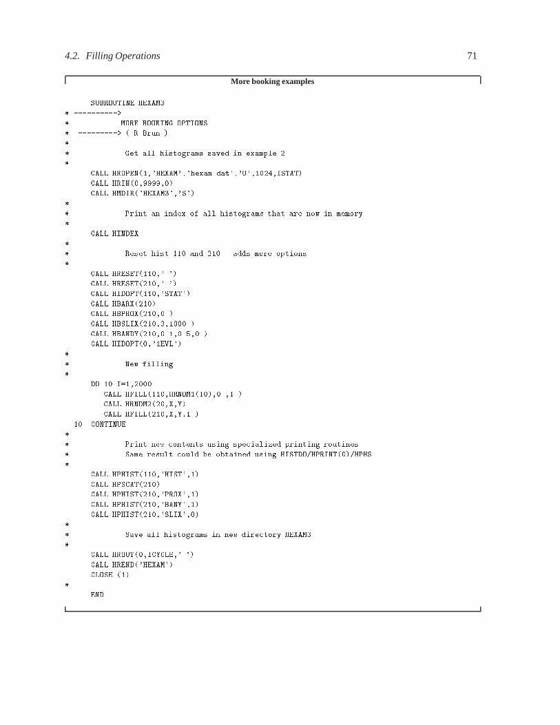
4.2. Filling Operations 71
More booking examples
SUBROUTINE HEXAM
������������
� MORE BOOKING OPTIONS
������������ � R�Brun �
Get all histograms saved in example �
CALL HROPEN���HEXAM��hexam�dat��U�����ISTAT�
CALL HRIN��������
CALL HMDIR��HEXAM��S��
Print an index of all histograms that are now in memory
CALL HINDEX
Reset hist ��� and ���� adds more options
CALL HRESET����� ��
CALL HRESET����� ��
CALL HIDOPT�����STAT��
CALL HBARX�����
CALL HBPROX�������
CALL HBSLIX����������
CALL HBANDY�������������
CALL HIDOPT����EVL��
New filling
DO �� I������
CALL HFILL����HRNDM����������
CALL HRNDM����XY�
CALL HFILL����XY���
�� CONTINUE
Print new contents using specialized printing routines
Same result could be obtained using HISTDO�HPRINT����HPHS�
CALL HPHIST�����HIST���
CALL HPSCAT�����
CALL HPHIST�����PROX���
CALL HPHIST�����BANY���
CALL HPHIST�����SLIX���
Save all histograms in new directory HEXAM
CALL HROUT��ICYCLE� ��
CALL HREND��HEXAM��
CLOSE ���
END

72 Chapter 4. Advanced features for booking and editing operations
Output Generated
������������������������������������������������������������������������������������������������������������������������������ �� HBOOK HBOOK CERN VERSION ���� HISTOGRAM AND PLOT INDEX �������� �� ������������������������������������������������������������������������������������������������������������������������������� �� NO TITLE ID B�C ENTRIES DIM NCHA LOWER UPPER ADDRESS LENGTH �� ������������������������������������������������������������������������������������������������������������������������������� �� �� � TEST OF HRNDM� � �� � � X � �E� ��E�� ����� ��� �� �� �� � TEST OF HRNDM� � �� � � X � �E� ��E�� ����� ��� �� �� �� � THIS HISTOGRAM IS FILLED ACCORDING TO TH �� � � X � �E� ��E�� ��� �� �� E FUNCTION HTFUN� �� �� � TEST OF HRNDM� � �� � � X � �E� ��E�� �� �� ���� �� Y � �E� ��E�� ���� ���� �� �� TEST OF HRNDM� � �� � � X � �E� ��E�� ���� ���� �� Y � �E� ��E�� ��� ���� �� �� � HIST FILLED WITH HFILL AND HRNDM� �� � X � �E� ��E�� � � ��� �� Y � �E� ��E�� ��� ��� �� ������������������������������������������������������������������������������������������������������������������������������
MEMORY UTILISATION
MAXIMUM TOTAL SIZE OF COMMON �PAWC� �
THIS HISTOGRAM IS FILLED ACCORDING TO THE FUNCTION HTFUN�
HBOOK ID � �� DATE �������� NO � �
�� �� I �� I II�� I II� I I I � I I I � II I � I I � I I I I�� I I�� I I�� I I �� I I I� I I I �� I I I I�� I I I I I �� I II I I I I�� I I II I I I� I I I II I I II�� I I I II I I II �� I I I I I I I II I�� I I I I I I I II II �� II I I II I III I I� I I I II III�� I I I I I I �� I I II I II I I�� II I I I I II I II�� I II I I I I II I� I II I II I I � I II III III� I II I� II I� II I
CHANNELS � �� � � � � � � � � � ���� �������� �������� �������� �������� �������� �������� �������� �������� �������� ����
CONTENTS � ���������� � ��� ���������� � � �� ������������������������������������� � �� �� ���������������� �������� ��� ��� ��� �� ������������ ���� ��������������������
LOWEDGE �� ���������������������������������������� �������������������������������������������� � ���� �������� �������� �������� �������� �������� �������� �������� �������� �������� ����
� ENTRIES � � � ALL CHANNELS � ��E�� � UNDERFLOW � �E� � OVERFLOW � �E�� BIN WID � ��E� � MEAN VALUE � �����E� � R � M � S � ����E� � NEQUIVAL � ��E��
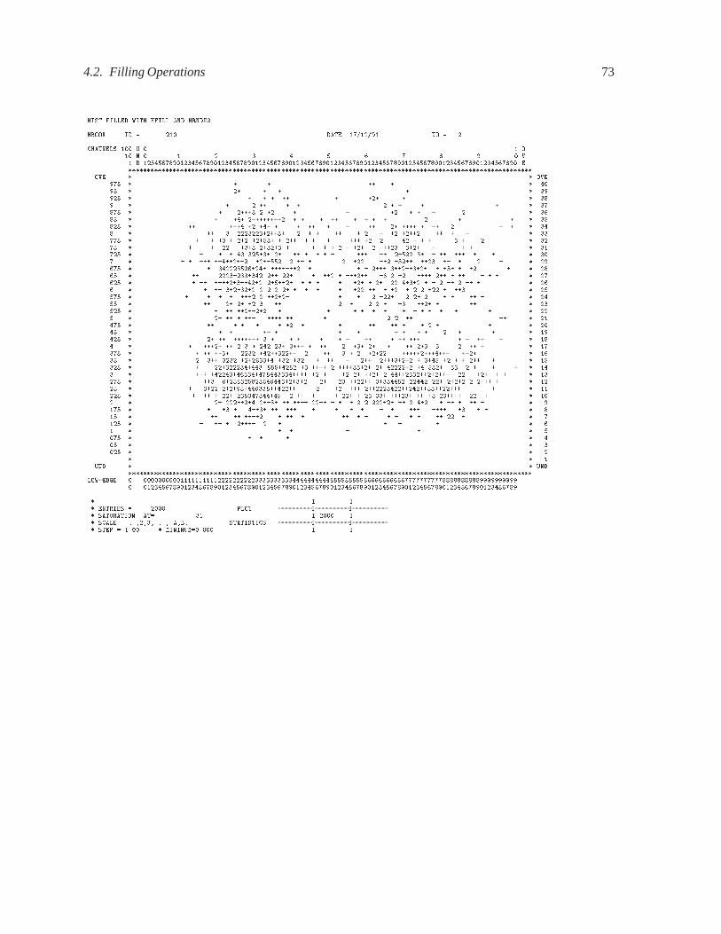
4.2. Filling Operations 73
HIST FILLED WITH HFILL AND HRNDM�
HBOOK ID � �� DATE �������� NO � �
CHANNELS � U � O� N � � � � � � � � V� D ���� �������� �������� �������� �������� �������� �������� �������� �������� �������� ���� E������������������������������������������������������������������������������������������������������������
OVE � � OVE��� � � � �� � � ��� � �� � � � � ����� � � � � �� � ��� � � ���� � � � �� � � � � � � � � ����� � � ����� � �� � � �� � � � � � ���� � � ��� ���������� � � � �� � � � � � � � � � ��� � �� ���� �� ��� � � �� � � �� �� ���� � �� � � � � ���� � �� � ������������� � � � �� � � � �� ����� �� � � � ����� � � � �� � ��� ��� �� � ��� � � � ��� �� � �� � � � � � � � ���� � � � �� ���� ������ � � � � � � ��� � ����� ���� � � � � ����� � � � � �� �� ��� �� �� � � � � ��� �� �� �� �� � �� ��� � � � ��� � � � ��� ��������� ���� � � �� � � ��� ��� ����� ���� �� � � � � ����� � � ������ ������ �������� � � � ���� ���������� � ��� � �� � � ���� � �� ������������ ��� ��� � ��� � ������ �� � �� ���� ��� � �� � � � � ����� � � �� ������������� �� ���� � � � � ��� � �� �� ����� � � � �� � �� � � ���� � � �� �������� � � � �� � � � � ��� �� � �� � � � ��� � ��� � � � � � � � � � ���� � ������ � � � ���� � �� � � � �� � � ��� � �� �� �� �� � �� � � � � � �� ���� � �� � ��� � � � �� �������� � � � � � � � � � � � � � � ��� � �� �� � ��� ���� �� � � � �� �� � ����� � �� � � � � �� � � �� �� � � � � � � ��� � � � �� � � � � � � � � � � � ����� � �� �� ������� � � � � � � � �� � �� ��� � � �� � � ���� � � ����� �� � � � ��� ��� ���� � �� � ��� �� � �� ��� � � �� � � ����� � � �� ���� ���� ���������� � �� � � � ����� ������������� ���� � ���� � � ��� ���� ��������� ��� ��� � �� � ��� ��������� � ��� �� � � ��� � � � ��� � � ������������� ��� � �� ���� � ��������� �� ������� �� ��� �� � � � � � ���� � ��� ��������������� ���������� �� � �� �� ���� � ���������������� �� ��� � � � ����� � ��� ��� �� ��������������� �� �� ������ ������ � ����� ��� ����� � ���� � � ���� � � ���������� ������ ������� � �� ���� ����������������� �������� � � ����� � � �� � ������ �������� � �� � � ����� �� ������������� �� ������ ��� � � ��� � �� �������� ����� �� ���� ���� � � � � � ������ �� � ��� � �� � �� � � ���� � � �� � ����� �� ��� � � � � � � ��� ���� �� � � � ��� � �� �� ����� � �� � �� � � � � � � �� �� � � ���� � � �� � ����� � � � � � � ��� � � � � � � �� � � � � � �� � � ��� � � �
� � �UND � � UND
������������������������������������������������������������������������������������������������������������LOWEDGE ���������������������������������������� ����������������������������������������
���� �������� �������� �������� �������� �������� �������� �������� �������� �������� ����
� I I� ENTRIES � � PLOT II� SATURATION AT� �� I � I� SCALE ������������ A�B� STATISTICS II� STEP � �� � MINIMUM�� I I
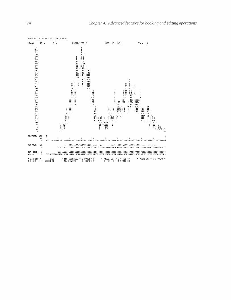
74 Chapter 4. Advanced features for booking and editing operations
HIST FILLED WITH HFILL AND HRNDM�
HBOOK ID � �� PROJECTION X DATE �������� NO � �
�� I�� I�� I� I I�� I II�� I II II�� II II II�� II II I� I II II � II IIII � III IIII I � IIII IIII II � IIII I III II IIII�� I I I III I�� I I I II I�� II I I III II I�� II I III II I� II I I II I I�� III I I I I I I I I�� IIII III I I II I I I�� III III I I II IIIII II�� I I I II IIII I� II II II I II IIIIIIIII�� II II III I II III I I III�� II I III IIIIIII I III IIIII�� I I IIII I I II II�� I II I I I III I I I II II II� I II I II I IIII I I II IIII I�� I III II IIIII IIIII I�� III III I II I I I IIIII I�� II I I II I IIII I IIII II I�� I I I I I I III I I II III� I I IIIIIII I I� I I II IIII I II I� II I I I I IIII� I I I I I II I� I II II
CHANNELS � �� � � � � � � � � � ���� �������� �������� �������� �������� �������� �������� �������� �������� �������� ����
CONTENTS � ��������� � � �� ���������� �� � ���������������������������������� �� ��� �� �� ��������������� ��������������� ������������������������������ ���� ������
LOWEDGE �� ���������������������������������������� �������������������������������������������� � ���� �������� �������� �������� �������� �������� �������� �������� �������� �������� ����
� ENTRIES � � � ALL CHANNELS � ��E�� � UNDERFLOW � �E� � OVERFLOW � �E�� BIN WID � ��E� � MEAN VALUE � �����E� � R � M � S � ����E�

4.2. Filling Operations 75
HIST FILLED WITH HFILL AND HRNDM�
HBOOK ID � �� BAND Y DATE �������� NO � �
BAND Y NO � � XMIN� ��E� XMAX� � E�
�� �� II� II�� II�� II�� I I�� I I� I I � I I � I I�� I I �� I I I� I I I I�� I I I I �� I I I III�� I I I I�� I I I I� I I I I�� I I I I�� I I I I� I II I� I I
CHANNELS � � � � �� ���� �������� �������� �������� ����
CONTENTS � ��������� ��� ������������������� ������������ ������������� � �
LOWEDGE �� ���������������� �������������������� � � �� �� �� �� �� �� �� �� �� �
� ENTRIES � ��� � ALL CHANNELS � ����E�� � UNDERFLOW � �E� � OVERFLOW � �E�� BIN WID � �� E� � MEAN VALUE � ���E� � R � M � S � �����E�
HIST FILLED WITH HFILL AND HRNDM�
HBOOK ID � �� SLICE X DATE �������� NO �
SLICE X NO � � YMIN� �E� YMAX� �����E�
�� I�� I�� I�� I� I I�� I I I�� I I I�� I II II�� I II III� I II III�� II II II I�� II IIIIII I�� II I IIIIII�� II I IIIIII� III IIIIIII I I�� I III II III I I�� II II I III I I I�� II I II I III I I I I I�� IIII I I III II I II I � I III I I III II I I III III I�� I III I I II II I I I IIIII II I�� I III I I I I I IIIII III I�� I III I II I I IIIII IIII IIII I�� I II III I IIII III I I III I I� III II III II I II III I I IIIIIII II� I III I I II II III II II II IIII I IIII II� I III I IIII II IIIIII III III I I IIIIIIIII I I� I I IIII II IIII II III II III III I I� II I I II I III I I I II IIIIIIII I III III I II IIII IIIII I I I I I III IIII� III IIII III III II I II I I III I� II I I I I I I I I IIIII I� II I II I I I IIIIII I� II I I I
CHANNELS � �� � � � � � � � � � ���� �������� �������� �������� �������� �������� �������� �������� �������� �������� ����
CONTENTS � � ���������������� �� � � � ����� ��� ��� ���������� �� ������������� �� ���� ����� ���� ����������������������� ������� �
LOWEDGE �� ���������������������������������������� �������������������������������������������� � ���� �������� �������� �������� �������� �������� �������� �������� �������� �������� ����
� ENTRIES � � � � ALL CHANNELS � �� �E�� � UNDERFLOW � �E� � OVERFLOW � �E�� BIN WID � ��E� � MEAN VALUE � ����E� � R � M � S � �����E�
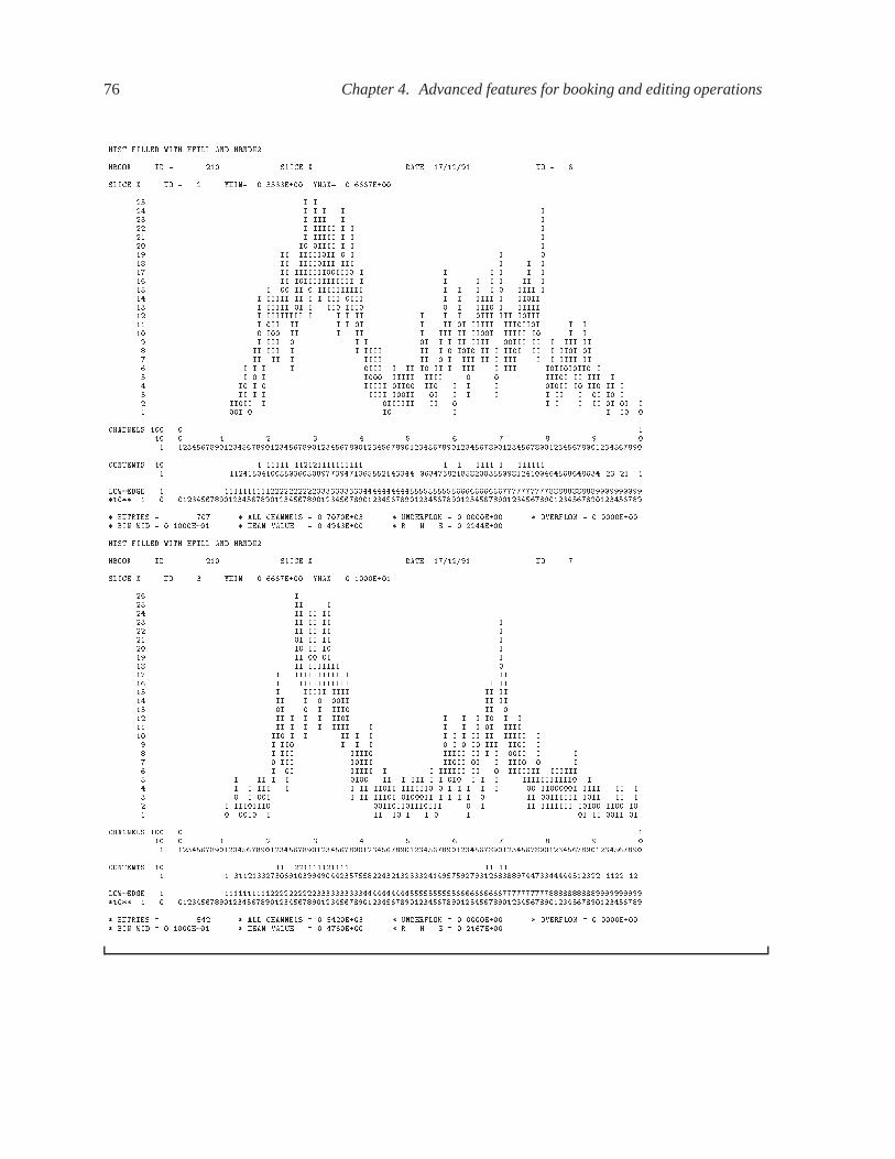
76 Chapter 4. Advanced features for booking and editing operations
HIST FILLED WITH HFILL AND HRNDM�
HBOOK ID � �� SLICE X DATE �������� NO � �
SLICE X NO � � YMIN� �����E� YMAX� �����E�
� I I�� I I I I I�� I III I I�� I IIIII I I I�� I IIIII I I I� I IIII I I I�� II IIIIIII I I �� II IIIIIII III I I I�� II IIIIIIIIII I I I I I I�� II IIIIIIIIIIII I I I I I II I� I II IIIIIIIIII I I I I IIII I�� I IIIII II I I III III I I IIII I IIII�� I IIIII I I II III I III I IIIII�� I IIIIIIII I I I II I I I III III IIII�� I II II I I I I II I IIIII IIIIII I I� I II I II I III II III IIIII I I I� I III I I I I I II IIII III II I III II� II III I I IIII II I II II I III II I III I� II II I IIII II I III II I III I I IIII II� I I I I III I II I II I III I III IIIIII I I I I IIIII IIII IIII II III I� I I IIIII II II I I I III I II II I� II I I IIII III I I I I I II I I I I� IIII I IIIIII II I I I II I I I� I I I I I
CHANNELS � �� � � � � � � � � � ���� �������� �������� �������� �������� �������� �������� �������� �������� �������� ����
CONTENTS � � ����� ��������������� � � ���� � �������� ����� �� ��� ����������� ������� ���������� ��� ����������� �������� �� �� �
LOWEDGE �� ���������������������������������������� �������������������������������������������� � ���� �������� �������� �������� �������� �������� �������� �������� �������� �������� ����
� ENTRIES � �� � ALL CHANNELS � ���E�� � UNDERFLOW � �E� � OVERFLOW � �E�� BIN WID � ��E� � MEAN VALUE � �����E� � R � M � S � �����E�
HIST FILLED WITH HFILL AND HRNDM�
HBOOK ID � �� SLICE X DATE �������� NO � �
SLICE X NO � � YMIN� �����E� YMAX� ��E��
�� I� II I�� II II II�� II II II I�� II II II I�� I II II I� I II I I�� II I I�� II IIIIIII �� I IIIIIIIIII I II�� I IIIIIIIIIII I II� I IIIII IIII II II�� II I II II II�� I I III II �� II I I I III I I I I I I�� II I I I IIII I I I I I IIII� II I I II I I I I I II II IIIII I� I II I I I I I III III I� I III IIII IIIII II I I II I I� III IIII IIII I I III I� I I IIIII I I IIIIII II IIIIIII IIIIII I II I I I II I III I I I I I I IIIIIIIIIII I� I I III I I II IIII IIIIII I I I I I III IIII II I� I I I II IIII III I I I I II IIIIII III II I� I IIIIII IIIIIIIIII I II IIIIIII II II I� I I II I I I I I II II I
CHANNELS � �� � � � � � � � � � ���� �������� �������� �������� �������� �������� �������� �������� �������� �������� ����
CONTENTS � �� ������������ �� ���� � ���������������������� � ����������������� � ������������������������ ����� ���� ��
LOWEDGE �� ���������������������������������������� �������������������������������������������� � ���� �������� �������� �������� �������� �������� �������� �������� �������� �������� ����
� ENTRIES � �� � ALL CHANNELS � � ��E�� � UNDERFLOW � �E� � OVERFLOW � �E�� BIN WID � ��E� � MEAN VALUE � ����E� � R � M � S � �����E�

4.3. Editing operations 77
4.3 Editing operations
Histograms are output on the line printer by calling HISTDO or HPRINT, according to the following spec-ifications:
One-dimensional histograms
One histogram per page is printed, writing the global title, date, title, drawing the contour of the histogramin the range between the minimum and the maximum content, with the contents scale adjusted to fit on onepage, followed by channel number, contents, and low edge of each channel, plus some statistics about thehistogram itself (entries, mean value, standard deviation and so on). If the number of channels is greaterthan 100, the histogram is printed on several pages.
Two-dimensional histograms
They can use more than one page, according to the number of channels in X and Y, and in X and Y bothchannel number and lower edge of each channel are printed.
The plot statistics reported at the bottom consists of a table of 9 numbers, corresponding to the total con-tents in each of the following classes:
N� N� N�
N� N N�
N� N� N
N� = underflow X , overflow Y
N� = X inside range , overflow Y
N� = overflow X , overflow Y
N� = underflow X , Y inside range
N = X inside range , Y inside range
N� = overflow X , Y inside range
N� = underflow X , underflow Y
N� = X inside range , underflow Y
N = overflow X , underflow YAny of these numbers can in fact be smaller than the real sum of the contents, in the case of saturation ofa cell.
For information on how to suppress the plot statistics, see HIDOPT�ID��NPST��
All projections, bands and slices follow the plot they refer to as 1-dimensional histograms in the order inwhich they were booked.
Histograms are printed with the channels oriented along computer printer output columns, so if they ex-tend to more than 100 channels they will be chopped into pieces of 100 channels each and printed oneafter the other on separate pages. The same is true for 2-dimensional histograms, the limit for tables beingrelated to the maximum value that has to be stored in each channel (see remarks about HTABLE).
Using the entries described in this chapter, it is possible to modify the standard output format, adding orsuppressing some information, choosing a different printed presentation, and modifying the mapping ofhistograms onto computer output pages.
One-dimensional histograms can also be printed with channels oriented along rows instead of columns,to avoid chopping up those having more than 100 channels.
All editing entries must be executed before calling HISTDO or HPRINT. Some of them can be executedany time after the booking, others require that the histogram is already full, so it is good practice to groupthem (perhaps in one single subroutine) and execute them just before printing.
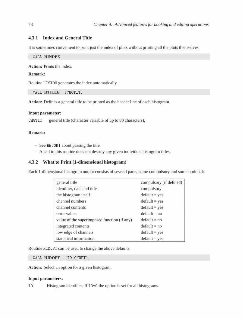
78 Chapter 4. Advanced features for booking and editing operations
4.3.1 Index and General Title
It is sometimes convenient to print just the index of plots without printing all the plots themselves.
CALL HINDEX
Action: Prints the index.
Remark:
Routine HISTDO generates the index automatically.
CALL HTITLE �CHGTIT�
Action: Defines a general title to be printed as the header line of each histogram.
Input parameter:
CHGTIT general title (character variable of up to 80 characters).
Remark:
– See HBOOK� about passing the title
– A call to this routine does not destroy any given individual histogram titles.
4.3.2 What to Print (1-dimensional histogram)
Each 1-dimensional histogram output consists of several parts, some compulsory and some optional:
general title compulsory (if defined)
identifier, date and title compulsory
the histogram itself default = yes
channel numbers default = yes
channel contents default = yes
error values default = no
value of the superimposed function (if any) default = no
integrated contents default = no
low edge of channels default = yes
statistical information default = yes
Routine HIDOPT can be used to change the above defaults.
CALL HIDOPT �ID�CHOPT�
Action: Select an option for a given histogram.
Input parameters:
ID Histogram identifier. If ID�� the option is set for all histograms.

4.3. Editing operations 79
CHOPT Character variable specifying the option chosen (see table 4.1.)
Option ActionSETD� Set all options to the default values
SHOW Print all the options currently setBLAC 1 Dim histogram printed with X characters (see HPCHAR)CONT� 1 Dim histogram is printed with the contour optionSTAR 1 Dim histogram is printed with a * at the Y value (see HPCHAR)SCAT� Print a 2 Dim histogram as a scatter-plotTABL Print a 2 Dim histogram as a tablePROS� Plot errors as the Spread of each bin in Y for profile histogramsPROE Plot errors as the mean of each bin in Y for profile histograms
STAT Mean value and RMS computed at filling time (double precision)NSTA� Mean value and RMS computed from bin contents onlyERRO Errors bars printed as SQRT(contents)NERR� Do not print print error barsINTE Print the values of integrated contents bin by binNINT� Do not print integrated contentsLOGY 1 Dim histogram is printed in Log scale in YLINY� 1 Dim histogram is printed in linear scale in YPCHA� Print channel numbers
NPCH Do not print channel numbersPCON� Print bin contentsNPCO Do not print bin contentsPLOW� Print values of low edge of the binsNPLO Do not print the low edgePERR Print the values of the errors for each binNPER� Do not print the values of the errorsPFUN Print the values of the associated function bin by binNPFU� Do not print the values of the associated function
PHIS� Print the histogram profileNPHI Do not print the histogram profilePSTA� Print the values of statistics (entries,mean,RMS,etc.)NPST Do not print values of statisticsROTA Print histogram rotated by 90 degreesNROT� Print histogram vertically�EVL Force an integer value for the steps in the Y axisAEVL� Steps for the Y axis are automatically computed
�PAG Histogram is printed over two pages�PAG� Histogram is printed in one single page
A star ��� indicates that the option is the default setting.
Table 4.1: List of available HBOOK options, which can be set by HIDOPT

80 Chapter 4. Advanced features for booking and editing operations
CALL HSTAF �CHOPT�
If CHOPT��YES� statisticsare computed at filling time. All the histogramscreated (viaHBOOK� orHBOOK�)after a CALL HSTAF��YES��, will have the IDOPT option �STAT� automatically activated. This is veryuseful when histograms are created in an indirect way like in the command NT�PLOT. The way to activatethis option in paw is:
PAW � OPTION HSTA
PAW � NT�PLOT ���x IDH����
4.3.3 Graphic Choices (1-dimensional histogram)
A histogram is normally represented by drawing its contour, with a channel being represented by onecharacter along the printed line at a displacement corresponding to the bin contents, but alternative graphicpresentations are available. If some contents are negative a dotted line is drawn at Y��.
CALL HPCHAR �CHOPT�CHAR�
Action: Selects a printing character different from the default for histograms that are not drawn contouronly, or for superimposed functions.
Input parameters:
CHOPT Printing option for which the character applies. It can be:
�BLAC� when HIDOPT�ID��BLAC�� is called�FUNC� when HBFUN�, HFUNC or HIDOPT�ID��STAR�� have been called.�STAR� when HBFUN�, HFUNC or HIDOPT�ID��STAR�� have been called.
CHAR Character chosen.
Example:
CALL HPCHAR ��STAR�����
Replaces the asterisk with a dot in all histograms with the HIDOPT�ID��STAR�� option selected.
CALL HBIGBI �ID�NCOL�
Action: For a given 1-dimensional histogram prints one channel over a certain number of columns.
Input parameters:
ID Histogram identifier
NCOL Number of columns to be used per bin.NCOL�� meams use the full width of the page.
Remark:
– HBIGBI will be applied to histograms output across the page only, i.e. if NCHAN�NCOL����.If this relation is not fulfilled, then the value of NCOLwill be reduced till it obeys the inequality. Norestrictions if the histogram is printed down the page (HIDOPT�ID��ROTA��).
– If the histogram is 2-dimensional, the “bigbin” option is selected on all its projections, etc.
– It can be redefined at any time.

4.3. Editing operations 81
4.3.4 Scale Definition and Normalization
Note that, whenever a multiplication by a power of ten appears in the output, it means that the quantity itrefers to has been multiplied by that factor before being printed.
The scaling of the contents while outputing a 1-dimensional histogram is chosen by default to be linearand to span the interval between the minimum and the maximum of the contents of the channels.
The options described below allow:
– the choice of a logarithmic contents scale
– the definition of the limits of the scale
– the choice of the minimum step of the scale to be an integer
– the choice of the same scale for several histograms so that they can be compared more easily
– the normalisation of the total contents to a given value
If the identifier corresponds to a 2-dimensional histogram, they act on projections, slices, bands if any.
CALL HMAXIM �ID�FMAX� and CALL HMINIM �ID�FMIN�
Action: The scale limits for a histogram are not calculated automatically, but they as set to the specifiedvalues. The histogram contents are left intact.
Input parameters:
ID Histogram identifier.ID�� Meams apply limit to all existing histograms.
FMAX�FMIN� Maximum (minimum) for contents scale of given histogram.When FMAX�FMIN then the maximum and minimum values of the scale are computedautomatically.
These routines can be called as often as desired for a given histogram.
CALL HCOMPA �IDVECT�N�
Action: Compare the contents of all histograms whose identifiers are contained in array IDVECT and as-sign them the same vertical scale. The comparison is made on the basis of the contents at the time routineis called.
Input parameters:
IDVECT Array of N elements that contain the identifiers of the histograms to be compared The arraymust be dimensioned in the calling program to a length larger or equal to N.
N Number of histograms to be comparedN�� Means compare all existing 1-dimensional histograms.
Remark:
This routine can be called as often as desired to recompute the histogram scales.

82 Chapter 4. Advanced features for booking and editing operations
CALL HNORMA �ID�XNORM�
Action: Normalizes the total contents of a 1-dimensional histogram when printing it. Original contentsare left intact.
Input parameters:
ID Histogram identifierID�� Meams apply normalization factor to all existing histograms
XNORM Normalization factor to be applied to histogram when printing.XNORM�� is illegal.
Remarks:
– If a function is superimposed, it is not affected by the normalization
– The histogram can have error bars
– The normalization factor can be redefined at any time.
CALL HSCALE �ID�FACTOR�
Action: The contents scale for a scatter plot is multiplied by a given factor.
Input parameters:
ID Histogram identifierID�� Means apply scaling factor to to all existing 2-dimensional histograms.
FACTOR Scaling factor to be applied to the contents scale.FACTOR�� means automatic scaling. The range will be from the minimum to the maximumof the actual contents.
In a scatter-plot the contents scale starts at �� and increases in steps of �. The content of each channel isrepresented by one character, using the following scheme:
Value Character Range� � � x � �
� � � � x � �
� � � � x � �
� � � � x � ���
���...
� x � ��
�� A �� � x � ��
�� B �� � x � ��
�� C �� � x � �����
���...
overflow � VMX � x

4.3. Editing operations 83
Remarks:
– The call has no effect on the projection of histogram ID.
– The scale can be redefined several times.
4.3.5 Page Control
Plots are output on the line printer file, each of them starting at the beginning of a new page. The pagesize is an installationdefault. One dimensional histograms take one page, and are printed across the page.
All those defaults can be overwritten as follows.
CALL HSQUEZ ��YES���NO��
Action: Suppres / reestablish page eject.
CALL HPAGSZ �NLINES�
Action: Changes the number of lines per page.
Input parameter:
NLINES Number of lines per page. The initial value of this parameter is system dependent (generally56).
4.3.6 Selective Editing
Editing routines that draw histograms use a considerable amount of core, due to the complexity of thetasks they have to perform.
If the editing is performed by HISTDO or HPRINT, all the routines that deal with 1-dimensional histograms,rotated 1-dimensional histograms, 2-dimensional histograms, get loaded even if not used (e.g. even in thecase where only 1-dimensional in standard format are required).
In such cases, selective editing options for different classes can be used to replace HISTDO or HPRINT.
CALL HPHIST �ID�CHOICE�NUM�
Action: Edits 1-dimensional histogram or projection, slice or band of a 2-dimensional histogram on theline printer, in the standard representation.
Input parameters:
ID Histogram identifier. ID�� means edit all existing histograms.
CHOICE Character variable that selects subhistograms (irrelevant for the one-dimensional case). Seeroutine HUNPAK for possible values.CHOICE�� � is equivalent to CHOICE��HIST�
NUM Serial order of the slice or band. NUM�� is the same as NUM��
Routine HPHIST ignores the option HIDOPT�ID��ROTA��

84 Chapter 4. Advanced features for booking and editing operations
CALL HPROT �ID�CHOICE�NUM�
Action: Analogous to HPHIST, but with a presentation down the page. Parameters, special values andremarks are the same as for HPHIST.
CALL HPSCAT �ID�
Action: Edits a 2-dimensional histogram as a scatter-plot.
Input parameter:
ID Histogram identifier (2-dimensional).ID�� means to edit all histograms.
Remark:
– The 2-dimensional histogram with identifier IDmight have been booked as a table and will be out-put as a scatter-plot
– Projections are not printed, see HPHS.
CALL HPTAB �ID�
Action: Edits a 2-dimensional histogram as a table.
Input parameter:
ID Histogram identifier (2-dimensional).ID�� means to edit all histograms.
Remark:
– The 2-dimensional histogram with identifier ID might have been booked as a scatterplot but it willbe output as a table.
The following two routines can be used to save space when the program does not print tables and rotated1-dimensional histograms.
CALL HPHS �ID�
Action: Analogous to HPRINT, but ignore tables and HIDOPT�ID��ROTA��.
CALL HPHST �ID�
Action: Analogous to HPRINT, but ignore HIDOPT�ID��ROTA��.

4.3. Editing operations 85
4.3.7 Printing after System Error Recovery
The operating systems of some computers define CP time limits for job execution, and abort the job witha system error when this occurs. In most of the cases, users recover from the time limit error transferingcontrol to a summary subroutine that will eventually edit the histograms, calling, e.g. HISTDO. This canbe inconvenient if the time limit condition has been reached in HISTDO or other printing routines, becausethe printing will restart from the beginning. To avoid this, HBOOK can be instructed to start printing justwhere it stopped before.
CALL HPONCE
Action: In case of system error recovery during histogram editing, a possible recovery editing will startwhere the original printing stopped.
Remark:
If HPONCE has been called before printing, then a histogram that has been output completely will no longerbe printed.
4.3.8 Changing Logical unit numbers for output and message files
The output file, containing the histograms, is by default the line printer file, where also error messageswill be written.
The names of the result and error files can be redefined using:
CALL HOUTPU �LOUT� and CALL HERMES �LERR�
Action: Replaces the logical unit value for the results (HOUTPU) or the error messages (HERMES).
Input parameters:
LOUT logical unit number of the file with the printed output
LERR logical unit number of the file with error messages
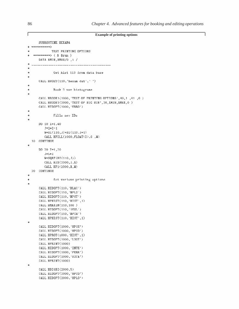
86 Chapter 4. Advanced features for booking and editing operations
Example of printing options
SUBROUTINE HEXAM�
������������
� TEST PRINTING OPTIONS
������������ � R�Brun �
DATA XMINXMAX������
��������������������������������������������
Get hist ��� from data base
CALL HRGET�����hexam�dat�� ��
Book � new histograms
CALL HBOOK�������TEST OF PRINTING OPTIONS�����������
CALL HBOOK�������TEST OF BIG BIN���XMINXMAX���
CALL HIDOPT������ERRO��
Fills new IDs
DO �� I����
J�� I��
W�HI����J��HI����J���
CALL HFILL�����FLOAT�I���W�
�� CONTINUE
DO �� I����
J�� I
W�SQRT�HI����J��
CALL HIX�����IX�
CALL HF������XW�
�� CONTINUE
Set various printing options
CALL HIDOPT�����BLAC��
CALL HIDOPT�����NPLO��
CALL HIDOPT�����NPST��
CALL HPHIST�����HIST���
CALL HMAXIM���������
CALL HIDOPT������EVL��
CALL HIDOPT�����NPCH��
CALL HPHIST�����HIST���
CALL HIDOPT������NPCH��
CALL HIDOPT������NPCO��
CALL HPROT������HIST���
CALL HIDOPT������LOGY��
CALL HPRINT������
CALL HIDOPT������INTE��
CALL HIDOPT������PERR��
CALL HIDOPT������ROTA��
CALL HPRINT������
CALL HBIGBI�������
CALL HIDOPT������NPCO��
CALL HIDOPT������NPLO��

4.3. Editing operations 87
CALL HPRINT������
END
Output Generated
THIS HISTOGRAM IS FILLED ACCORDING TO THE FUNCTION HTFUN�
HBOOK ID � �� DATE �������� NO � �
��� ���� X��� X�� �X� � XX � � XX X��� XXXX���� � XXXXX�� XXXXXXX ��� XXXXXXXX��� XXXXXXXX��� XXXXXXXX���� XXXXXXXXX�� XXXXXXXXXX��� XXXXXXXXXXX��� XXXXXXXXXXX�� XXXXXXXXXXX�� XXXXXXXXXXX�� XXXXXXXXXXXXX�� XXXXXXXXXXXXX ��� XXXXXXXXXXXXX�X�� XXXXXXXXXXXXXXXX�� XXXXXXXXXXXXXXXX � �� XXXXXXXXXXXXXXXX X � X X �� XXXXXXXXXXXXXXXX X X�X �X X X�� XXXXXXXXXXXXXXXX XX XXX� XX X X ��� XXXXXXXXXXXXXXXX�XX � XXXX�XXXX�XXXX�� XXXXXXXXXXXXXXXXXXX � X XXXXXXXXXXXXXX�� X XXXXXXXXXXXXXXXXXXX XXX �XXXXXXXXXXXXXXX � XXXXXXXXXXXXXXXXXXXXX XXX�XXXXXXXXXXXXXXXX � XXXXXXXXXXXXXXXXXXXXXX X XXXXXXXXXXXXXXXXXXXX�X�� XXXXXXXXXXXXXXXXXXXXXX� XXXXXXXXXXXXXXXXXXXXXXXX�� XXXXXXXXXXXXXXXXXXXXXXXX XXXXXXXXXXXXXXXXXXXXXXXX X� XXXXXXXXXXXXXXXXXXXXXXXX� �XXXXXXXXXXXXXXXXXXXXXXXXXX X�� XXXXXXXXXXXXXXXXXXXXXXXXX XXXXXXXXXXXXXXXXXXXXXXXXXXX �XX�� XXXXXXXXXXXXXXXXXXXXXXXXX � XXXXXXXXXXXXXXXXXXXXXXXXXXXXXXX�� �XXXXXXXXXXXXXXXXXXXXXXXXX� X � �XXXXXXXXXXXXXXXXXXXXXXXXXXXXXXXX� X�� �XXXXXXXXXXXXXXXXXXXXXXXXXXXX�X X X� XXXXXXXXXXXXXXXXXXXXXXXXXXXXXXXXXX X� � XXXXXXXXXXXXXXXXXXXXXXXXXXXXXXX X XX XXXXXXXXXXXXXXXXXXXXXXXXXXXXXXXXXXXXXX ��� XXXXXXXXXXXXXXXXXXXXXXXXXXXXXXXX XXXXXXXXXXXXXXXXXXXXXXXXXXXXXXXXXXXXXXXXXXX�X�� �XXXXXXXXXXXXXXXXXXXXXXXXXXXXXXXXXXXXXXXXXXXXXXXXXXXXXXXXXXXXXXXXXXXXXXXXXXXXXX��� XXXXXXXXXXXXXXXXXXXXXXXXXXXXXXXXXXXXXXXXXXXXXXXXXXXXXXXXXXXXXXXXXXXXXXXXXXXXXXXXXX ���� �� XX XXXXXXXXXXXXXXXXXXXXXXXXXXXXXXXXXXXXXXXXXXXXXXXXXXXXXXXXXXXXXXXXXXXXXXXXXXXXXXXXXXXXXXXX
CHANNELS � �� � � � � � � � � � ���� �������� �������� �������� �������� �������� �������� �������� �������� �������� ����
CONTENTS � �������������� ������� ����� � �������� ��������������� ��� ���������������� ���������������� ��������������������������� �� ��� ���������� ����� ������ ���� ������������ ��� ����� ��

88 Chapter 4. Advanced features for booking and editing operations
THIS HISTOGRAM IS FILLED ACCORDING TO THE FUNCTION HTFUN�
HBOOK ID � �� DATE �������� NO � �
� XXXXXXXXXXXXX�� XXXXXXXXXXXXX ��� XXXXXXXXXXXXX�X�� XXXXXXXXXXXXXXXX�� XXXXXXXXXXXXXXXX � �� XXXXXXXXXXXXXXXX X � X X �� XXXXXXXXXXXXXXXX X X�X �X X X�� XXXXXXXXXXXXXXXX XX XXX� XX X X ��� XXXXXXXXXXXXXXXX�XX � XXXX�XXXX�XXXX�� XXXXXXXXXXXXXXXXXXX � X XXXXXXXXXXXXXX�� X XXXXXXXXXXXXXXXXXXX XXX �XXXXXXXXXXXXXXX � XXXXXXXXXXXXXXXXXXXXX XXX�XXXXXXXXXXXXXXXX � XXXXXXXXXXXXXXXXXXXXXX X XXXXXXXXXXXXXXXXXXXX�X�� XXXXXXXXXXXXXXXXXXXXXX� XXXXXXXXXXXXXXXXXXXXXXXX�� XXXXXXXXXXXXXXXXXXXXXXXX XXXXXXXXXXXXXXXXXXXXXXXX X� XXXXXXXXXXXXXXXXXXXXXXXX� �XXXXXXXXXXXXXXXXXXXXXXXXXX X�� XXXXXXXXXXXXXXXXXXXXXXXXX XXXXXXXXXXXXXXXXXXXXXXXXXXX �XX�� XXXXXXXXXXXXXXXXXXXXXXXXX � XXXXXXXXXXXXXXXXXXXXXXXXXXXXXXX�� �XXXXXXXXXXXXXXXXXXXXXXXXX� X � �XXXXXXXXXXXXXXXXXXXXXXXXXXXXXXXX� X�� �XXXXXXXXXXXXXXXXXXXXXXXXXXXX�X X X� XXXXXXXXXXXXXXXXXXXXXXXXXXXXXXXXXX X� � XXXXXXXXXXXXXXXXXXXXXXXXXXXXXXX X XX XXXXXXXXXXXXXXXXXXXXXXXXXXXXXXXXXXXXXX ��� XXXXXXXXXXXXXXXXXXXXXXXXXXXXXXXX XXXXXXXXXXXXXXXXXXXXXXXXXXXXXXXXXXXXXXXXXXX�X�� �XXXXXXXXXXXXXXXXXXXXXXXXXXXXXXXXXXXXXXXXXXXXXXXXXXXXXXXXXXXXXXXXXXXXXXXXXXXXXX��� XXXXXXXXXXXXXXXXXXXXXXXXXXXXXXXXXXXXXXXXXXXXXXXXXXXXXXXXXXXXXXXXXXXXXXXXXXXXXXXXXX ���� �� XX XXXXXXXXXXXXXXXXXXXXXXXXXXXXXXXXXXXXXXXXXXXXXXXXXXXXXXXXXXXXXXXXXXXXXXXXXXXXXXXXXXXXXXXX
CONTENTS � �������������� ������� ����� � �������� ��������������� ��� ���������������� ���������������� ��������������������������� �� ��� ���������� ����� ������ ���� ������������ ��� ����� ��
TEST OF PRINTING OPTIONS
HBOOK ID � � DATE �������� NO � �
� � � � � � � � � � � � � � � �� � � � � � � � � � � � � � � � � � ��� � � � � � � � � � � � � � � � � �
LOW EDGE IIIIIIIIIIIIIIIIIIIIII��� O� O IOI� OI� IOI� IOI� IOI
� IOI�� IOI�� IOI�� IOI�� IOI� IOI�� IOI�� IOI�� IOI�� IOI� IOI�� IOI�� IOI�� IOI�� IOI� IOI�� IOI�� IOI�� IOI�� IOI� IOI�� IOI�� IOI�� IOI�� IOI� IOI�� IOI�� IOI�� IOI�� IOI� IOI
LOW EDGE IIIIIIIIIIIIIIIIIIIIII
� � � � � � � � � � � � � � � �� � � � � � � � � � � � � � � � � � ��� � � � � � � � � � � � � � � � � �
� ENTRIES � � � ALL CHANNELS � �� �E�� � UNDERFLOW � �E� � OVERFLOW � �E�� BIN WID � ��E�� � MEAN VALUE � �����E�� � R � M � S � �� �E��

4.3. Editing operations 89
TEST OF PRINTING OPTIONS
HBOOK ID � � DATE �������� NO � ��
� ����� I������� I������� II I� ����� ������� I II���� �� ������� I II I II� ����� II����� � I II IIIII�� ���� II II������ I II � I ����� I I������ I I���� I ����� I ����� I I II ���� II������ I III������ I I I� ���� I I������ ������ I� ���� I���������� ������� I� ���� I����� ��� �� I����� II� I����� I����� II���� II���� I ���� II ��� I����� I����� I�� �� II����� II����� II�� �� II�����
LOWEDGE � ��������������������������������� ���� �������� �������� �������� ����
� ENTRIES � � � ALL CHANNELS � �� �E�� � UNDERFLOW � �E� � OVERFLOW � �E�� BIN WID � ��E�� � MEAN VALUE � �����E�� � R � M � S � �� �E��

90 Chapter 4. Advanced features for booking and editing operations
TEST OF PRINTING OPTIONS
HBOOK ID � � DATE �������� NO � ��
� � � � � � �� � � � � � � � � � � � ��� � � � � � � � � � � � � � � � � � � � � � � � � � � � � � � � � � � � � � � � � � � � � � � � � �
LOW EDGE INTEGRAT ERRORS IIIIIIIIIIIIIIIIIIIIIII��� � ����� OI� � ����� OI � ����� IOI� �� ����� IOI� �� ����� IOI� �� ��� IOI� �� ���� IOI� ��� �� �� IOI�� �� ���� IOI�� �� ������ IOI�� �� � ���� IOI�� �� ������ IOI� ���� ������ IOI�� ��� ������ IOI�� ��� ������ IOI�� �� � � ��� IOI�� ���� ������ IOI� ���� ������ IOI�� ��� ������ IOI�� ��� �� IOI�� ���� ����� IOI�� ���� ���� IOI� ��� ��� � IOI�� ���� ����� IOI�� ���� �� � IOI�� ��� ���� IOI�� ��� ���� IOI� ���� ���� IOI�� ���� ������ IOI�� ���� �� �� IOI�� � �� ������ IOI�� ���� ����� IOI� ���� ������ IOI�� ��� ����� IOI�� ���� ������ IOI�� ��� ����� IOI�� ���� ���� IOI� � � �� �� IOI
LOW EDGE INTEGRAT ERRORS IIIIIIIIIIIIIIIIIIIIIII
� � � � � � �� � � � � � � � � � � � ��� � � � � � � � � � � � � � � � � � � � � � � � � � � � � � � � � � � � � � � � � � � � � � � � � �
� ENTRIES � � � ALL CHANNELS � �� �E�� � UNDERFLOW � �E� � OVERFLOW � �E�� BIN WID � ��E�� � MEAN VALUE � �����E�� � R � M � S � �� �E��

4.3. Editing operations 91
TEST OF BIG BIN
HBOOK ID � � DATE �������� NO � ��
���� �� I I���� I I��� I I���� I I�� I I���� I I��� I I���� I I�� I I��� I I�� I I��� I I� I I��� I I�� I I��� I I� I I ��� I I I I�� I I I I��� I I I I� I I I I��� I I I I�� I I I I��� I I I I� I I I I��� I I I I�� I I I I��� I I I I� I I I I �� I I I I � I I I I �� I I I I I I I I��� I I I I�� I I I I��� I II I� I I��� I I�� I I��� I I� I I��� I I�� I I��� I I� I I��� I I�� I I��� I I� I I�� I I� I I�� I I
CHANNELS � � �� � � � � � � � � � � � � � � � �
� ENTRIES � � � ALL CHANNELS � �����E�� � UNDERFLOW � �E� � OVERFLOW � �E�� BIN WID � � E� � MEAN VALUE � �����E� � R � M � S � �����E�

Chapter 5: Accessing Information
The information contained in a histogram can be made available in local Fortran variables with the com-mands described below. It is possible to access channel contents (all together or individually) and alsomean value and standard deviation of 1-dimensional distributions.
5.1 Testing if a histogram exists in memory
LOGVAR � HEXIST �ID�
Action: Returns a logical value of �TRUE� if and histogram exists and �FALSE� otherwise.
Input parameter:
ID Histogram identifier
Remark:
HEXIST has to be declared LOGICAL in the calling routine.
5.2 List of histograms
CALL HID1 �IDVECT��N��
Action: Returns the number and identifiers of all existing 1-dimensional histograms.
Output Parameters:
IDVECT Array which will contain the histogram identifiers, in booking order. Its dimension should beat least equal to the number of 1-dimensional histograms.
N Number of 1-dimensional histograms.
CALL HID2 �IDVECT��N��
Action: Returns the number and identifiers of all existing 2-dimensional histograms. (see HID�).
CALL HIDALL �IDVECT��N��
Action: Returns the number and identifiers of all existing histograms. (see HID�).
5.3 Number of entries
CALL HNOENT �ID�NOENT��
Action: Provides the number of entries of a memory resident histogram, plot or Ntuple. N.B. The valuereturned includes also the contents of the overflow and underflow bins.
Input parameter:
ID Histogram identifier
Output Parameter:
NOENT Number of entries in the given histogram.
92
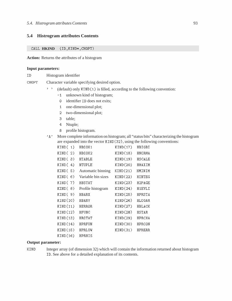
5.4. Histrogram attributes Contents 93
5.4 Histrogram attributes Contents
CALL HKIND �ID�KIND��CHOPT�
Action: Returns the attributes of a histogram
Input parameters:
ID Histogram identifier
CHOPT Character variable specifying desired option.
� � (default) only KIND��� is filled, according to the following convention:
�� unknown kind of histogram;
� identifier ID does not exits;
� one-dimensional plot;
� two-dimensional plot;
� table;
� Ntuple;
� profile histogram.
�A� More complete information on histogram; all “status bits” characterizing the histogramare expanded into the vector KIND����, using the following conventions:KIND� �� HBOOK� KIND���� HBIGBI
KIND� �� HBOOK� KIND���� HNORMA
KIND� �� HTABLE KIND��� HSCALE
KIND� �� NTUPLE KIND���� HMAXIM
KIND� � Automatic binning KIND���� HMINIM
KIND� �� Variable bin sizes KIND���� HINTEG
KIND� �� HBSTAT KIND���� H�PAGE
KIND� �� Profile histogram KIND���� H�EVLI
KIND� � HBARX KIND��� HPRSTA
KIND���� HBARY KIND���� HLOGAR
KIND���� HERROR KIND���� HBLACK
KIND���� HFUNC KIND���� HSTAR
KIND���� HROTAT KIND��� HPRCHA
KIND���� HPRFUN KIND���� HPRCON
KIND��� HPRLOW KIND���� HPRERR
KIND���� HPRHIS
Output parameter:
KIND Integer array (of dimension 32) which will contain the information returned about histogramID. See above for a detailed explanation of its contents.

94 Chapter 5. Accessing Information
5.5 Contents
CALL HUNPAK �ID�CONTEN��CHOICE�NUM�
Action: Transfer the contents of a histogram or a selected projection of a 2-dimensional histogram intoa local array.
Input parameters:
ID Histogram identifier
CHOICE Character variable selecting subhistograms (irrelevant for the 1-dimensional case)
�HIST� the 2-dimensional histogram itself. DefaultCHOICE�� � is equivalent to�HIST�.�PROX� X projection�PROY� Y projection�SLIX� X slice�SLIY� Y slice�BANX� X band�BANY� Y band
NUM Serial order of the slice or band that is requested. If NUM��, it is assumed to be �.
Output Parameter:
CONTEN Array to be dimensioned at least to the number of channels of the histogram (or projection),i.e. DIMENSION CONTEN�NX� in the 1-dimensional case and DIMENSION CONTEN�NX�NY�
in the 2-dimensional case.
VARIAB � HI �ID�I� and VARIAB � HIJ �ID�I�J�
Action: These functions return the channel contents in a given histogram bin in the 1-dimensional and2-dimensional case respectively.
Input parameters:
ID Histogram identifier.
I Bin number for X-coordinate. For I�� HI returns the number of underflows in X.
J (HIJ only) Bin number for Y-coordinate. For J�� HIJ returns the number of underflows in Y.
When NX� NY are respectively the number of channels in X and Y and I�NX��� J�NY��, then HI�HIJ
returns the number of overflows
VARIAB � HX �ID�X� and VARIAB � HXY �ID�X�Y�
Action: These functions return the channel contents in a given histogram of the bin which contains agiven value in X (1-dimensional case) or a given pair of �X�Y� (2-dimensional case).
Input parameters:
ID Histogram identifier
X X-value
Y Y-value (2-dimensional case, i.e. HXY only)

5.6. Errors 95
5.6 Errors
CALL HUNPKE �ID�CONTEN��CHOICE�NUM�
Action: Transfer the error contents of a histogram or a selected projection of a 2-dimensional histograminto the local array.
Input parameters:
ID Histogram identifier
CHOICE Character variable selecting subhistograms (irrelevant for the 1-dimensional case)
�HIST� the 2-dimensional histogram itself�PROX� X projection�PROY� Y projection�SLIX� X slice�SLIY� Y slice�BANX� X band�BANY� Y band
CHOICE�� � is equivalent to �HIST�.
NUM Serial order of the slice or band that is requested.If NUM��, it is assumed to be �.
Output Parameter:
CONTEN Array to be dimensioned at least to the number of channels of the histogram (or projection),i.e. DIMENSION CONTEN�NX� in the 1-dimensional case and DIMENSION CONTEN�NX�NY�
in the 2-dimensional case.
VARIAB � HIE �ID�I�
Action: Returns the value of the error that has been stored in a given 1-dimensional histogram channel.This corresponds to the square root of the sum of the squares of the weights.
Input parameters:
ID Histogram identifier.
I Channel (bin) number.
When HBARX has not been calledHIE returns the square root of the contents of the given channel.
VARIAB � HXE �ID�X�
Action: Analogous to HIE but referring to the channel that contains a given X-value.
Input parameters:
ID Histogram identifier.
X X-value.
The same remark as for HIE applies.

96 Chapter 5. Accessing Information
5.7 Associated function
VARIAB � HIF �ID�I�
Action: Function returning the value of the associated function that has been stored in a given histogramchannel. The function value will be zero if no associated function exists.
Input parameters:
ID Histogram identifier.
I Channel (bin) number.
5.8 Abscissa to channel number
CALL HXI �ID�X�I�� and CALL HXYIJ �ID�X�Y�I��J��
Action: Return the number of the channel (cell) which contains a given value in X (1-dimensional case)or a given pair of �X�Y� (2-dimensional case).
Input parameters:
ID Histogram identifier
X X-value
Y Y-value (2-dimensional case, i.e. HXYIJ only)
Output Parameters:
I Channel number in X-dimension.Under/Overflows give I�� or I�NCHANX�� respectively.
J Channel number in Y-dimension (2-dimensional case, i.e. HXYIJ only).Under/Overflows give J�� or J�NCHANY�� respectively.
CALL HIX �ID�I�X�� and CALL HIJXY �ID�I�J�X��Y��
Action: Returns the X-coordinate of the lower edge of a given channel (1-dimensional case) or the X-Ycoordinate pair if a given cell (2-dimensional case).
Input parameters:
ID Histogram identifier.
I Channel or cell number in X-dimension, with � � I � NCHANX.
J Cell number in Y-dimension with � � J � NCHANY. (2-dimensional case, i.e. HIJXY only)
Output Parameters:
X X-coordinate of lower edge of channel or cell.
Y Y-coordinate of lower edge of cell. (2-dimensional case, i.e. HIJXY only).

5.9. Maximum and Minimum 97
5.9 Maximum and Minimum
VARIAB � HMAX �ID� and VARIAB � HMIN �ID�
Action: Returns the maximum or minimum channel contents of a histogram (withoutunderflow and over-flow). In the case of a 2-dimensional histogram the returned value does not take into account projections.
Input parameter:
ID Histogram identifier.
5.10 Rebinning
CALL HREBIN �ID�X��Y��EX��EY��N�IFIRST�ILAST�
Action: The specified channels of a 1-dimensional histogram are cumulated (rebinned) into new bins.The final contents of the new bin is the average of the original bins.
Input parameters:
ID Histogram identifier
N Number of elements in the output arrays X�Y�EX�EY.
IFIRST First histogram channel on which the rebinning has to be performed.
ILAST Last histogram channel on which the rebinning has to be performed.
Output Parameters:
X Array containing the new abscissa values.
Y Array containing the cumulated contents.
EX Array containing the X errors.
EY Array containing the Y errors.
The abscissa errors on the rebinned histogram are calculated to be half the bin width.
If the standard deviation on the abscissa values is instead required, then specify N as a negative number.In this case, the returned abscissa error for each bin is the bin width divided by the square root of 12.
This routine may also be used for histograms with unequal bin widths.
Example:
CALL HREBIN �ID�X�Y�EX�EY��������
This call will regroup channels 11 to 85 three by three (25 bins) and return new abscissa, contents anderror values in the output arrays. In this case the errors in X will be equal to ���BINWIDTH.
CALL HREBIN �ID�X�Y�EX�EY�NCHAN���NCHAN�
This example shows a convenient way (using one subroutine call) to return the abscissa, contents anderrors for a 1-dimensional histogram. Note that in this case the errors in X are equal to ���BINWIDTH.

98 Chapter 5. Accessing Information
5.11 Integrated contents
VARIAB � HSUM �ID�
Action: Returns the integrated contents of a histogram (without underflow and overflow). In the case ofa 2-dimensional histogram the returned value does not take into account projections.
Input parameter:
ID Histogram identifier.
5.12 Histogram definition
CALL HGIVE �ID�CHTITL��NX��XMI��XMA��NY��YMI��YMA��NWT��LOC��
Action: Returns the booking parameters and address of a given histogram.
Input parameter:
ID Histogram identifier, cannot be zero.
Output Parameters:
CHTITL Histogram title (must be declared CHARACTER���)
NX Number of channels in X
XMI Lower edge of first X channel
XMA Upper edge of last X channel
NY Number of channels in Y (zero for a 1-dimensional histogram)
YMI Lower edge of first Y channel
YMA Upper edge of last Y channel
NWT Number of machine words for the title. If there is no title, NWT is returned as � .
LOC Address of the histogram in the common �PAWC�.
CALL HDUMP �ID�
Action: Prints a dump of the HBOOK storage area corresponding to a given histogram.
Input parameter:
ID Histogram identifier.ID�� will dump the whole of the HBOOK central memory storage area.

5.13. Statistics 99
5.13 Statistics
VARIAB � HSTATI �ID�ICASE�CHOICE�NUM�
Action: This function of type REAL returns the mean value, standard deviation or number of equivalentevents of a 1-dimensional distribution. Underflows and overflows are not included in the calculation.
Input parameters:
ID Histogram identifier
ICASE � Mean value� Standard deviation� Number of equivalent events
CHOICE See HUNPAK
NUM See HUNPAK
If HIDOPT�ID��STAT�� has been called, the results are based on the information stored at filling time.Otherwise the results are based on the channel contents only. If xi andwi represent the value and contentsof event i, then one has the following relations:
Expectation valueE�x� �
Pni��
wi xiPni�� wi
Mean value � E�x�
Central moment of order n, M�n� � E��x�E�x��n�
Standard deviation �qM���
Number of equivalent events ��Pn
i��wi�
�Pni��
w�
i

Chapter 6: Operations on Histograms
6.1 Arithmetic Operations
Histograms can be added, subtracted, divided or multiplied, provided their number of channels are thesame.
CALL HOPERA �ID��CHOPER�ID��ID��C��C��
Action: Fills an histogram I� with values such that, logically (operands are the bin contents)
ID� � C� � ID� �OPERATION� C� � ID�
Input parameters:
ID��ID� Operand histogram identifiers.
CHOPER Character variable specifying the kind of operation to be performed (�������);�B� compute binomial errors;�E� compute error bars on the resultinghistogramscorrectly, assuming that the inputhistogramsID� and ID� are independent.For instance �BE will generate binomial errors for the division of ID� by ID�.
ID� Identifier of the histogram containing the result after the operation.
C��C� Multiplicative constants.
Remark:
– ID�, ID� and ID� must have the same number of channels.
– If histogram ID� is not empty, its contents are overwritten
– The output histogram ID� can be either one of the input histograms ID� or ID�.
– If histogramID� does not exist, it is created by HOPERAwith the same specification as for histogramID�.
– The mean value, standard deviation, etc. are calculated from the contents of the resulting histogramID�, unless the �STAT� option is active and the operation is an addition or subtraction, in whichcase they are computed exactly.
– A division by zero gives zero.
– Negative results for bin contents in a packed histogram are meaningless
– The number of entries in the resulting histogram ID� is set to the sum of the entries in histogramsID� and ID�.
– When an operation is performed on two 1-dimensional histograms with the sum of the squares ofthe weights stored (option HBARX), the error on the resulting histogram is calculated supposing thatthe contents of the two input histograms ID� and ID� are uncorrelated. This is valid also for pro-jections, slices and bands of 2-dimensional histograms.
– If histogram ID� is packed the number of bits allocated per channel (cell) has to be sufficient tostore the results.
100

6.2. Statistical differences between histograms 101
6.2 Statistical differences between histograms
CALL HDIFF �ID��ID��PROB��CHOPT�
Action: Statistical test of compatibility in shape between two histograms using the Kolmogorov test. Thehistograms are compared and the probability that they could come from the same parent distribution iscalculated.
The comparison may be done between two 1-dimensional histograms or between two 2-dimensional his-tograms. For further details on the method, see 6.2.2 below.
Input parameters:
ID� Identifier of first histogram to be compared.
ID� Identifier of second histogram to be compared.
CHOPT A character string specifying the options desired.
�D� Debug printout, produces a blank line and two lines of information at each call, in-cluding the identifier numbers ID, the number of events in each histogram, the valueof PROB, and the maximum Kolmogorov distance between the two histograms. For 2-dimensional histograms, there are two Kolmogorov distances (see below). If option�N� is specified, there is a third line of output giving the probalilityPROB for shape andnormalization alone separately.
�F�� Histogram ID� has no errors (it is a function).
�F�� Histogram ID� has no errors (it is a function).
�N� Include a comparison of the relative normalization of the two histograms, in additionto comparing the shapes. The output parameter PROB is then a combined confidencelevel taking into account absolute contents.
�O� Overflow, requests that overflow bins be taken into account (also valid for 2-dim).
�U� Underflow, requests that underflow bins be taken into account (also valid for 2-dim).
For 2-dimensional histograms only�L� Left, include X-underflows in the calculation.
�R� Right, include X-overflows in the calculation.
�B� Bottom, include Y-underflows in the calculation.
�T� Top, include Y-overflows in the calculation.
Output Parameter:
PROB The probability of compatibility between the two histograms.
Remark:
– Options �O� and �U� can also refer to 2-dimensional histograms, so that, for example the string�UT� means that underflows in X and Y and overflows in Y should be included in the calculation.
– The histograms ID� and ID�must exist and already have been filled before the call to HDIFF. Theymust also have identical binning (lower and upper limits as well as number of bins).

102 Chapter 6. Operations on Histograms
– The probabilityPROB is returned as a number between zero and one. A values close to one indicatesvery similar histograms, and a value near zero means that it is very unlikely that the two arose fromthe same parent distribution.
– By default (no options selected with CHOPT) the comparison is done only on the shape of the twohistograms, without consideration of the difference in number of events, and ignoringall underflowand overflow bins.
6.2.1 Weights and Saturation
Weighted 1-dimensional histograms
It is possible to compare weighted with weighted histograms, and weighted with unweighted histograms,but only if HBOOK has been instructed to maintain the necessary information by appropriate calls (beforefilling) to HBARX. However it is not possible to take into account underflow or overflow bins if the eventsare weighted.
Saturated 1-dimensional histograms
If there is saturation (more than the maximum allowed contents in one or more bins), the probabilityPROBis calculated as if the bin contents were exactly at their maximum value, ignoring the saturation. Thisusually will result in a higher value of PROB than would be the case if the memory allowed the full contentsto be stored, but not always. It should therefore be realized that the results of HDIFF are not accurate whenthere is saturation, and it is the user’s responsability to avoid this condition.
2-dimensional histograms
Routine HDIFF cannot work if the events are weighted, since, in the current version of HBOOK, the neces-sary information is not maintained. HDIFF will also refuse to compare 2-dimensional histograms if thereis saturation, since it does not have enough information in this case.
6.2.2 Statistical Considerations
The Kolmogorov Test
The calculations in routine HDIFF are based on the Kolmogorov Test (See, e.g. [11], pages 269-270). Itis usually superior to the better-known Chisquare Test for the following reasons:
– It does not require a minimum number of events per bin, and in fact it is intended for unbinned data(this is discussed below).
– It takes account not only of the differences between corresponding bins, but also the sign of thedifference, and in particular it is sensitive to a sequence of consecutive deviations of the same sign.
In discussing the Kolmogorov test, we must distinguishbetween the two most important properties of anytest: its power and the calculation of its confidence level.

6.2. Statistical differences between histograms 103
The Power
The job of a statistical test is to distinguishbetween a null hypothesis (in this case: that the two histogramsare compatible) and the alternative hypothesis (in this case: that the two are not compatible). The powerof a test is defined as the probability of rejecting the null hypothesis when the alternative is true. In ourcase, the alternative is not well-defined (it is simply the ensemble of all hypotheses except the null) so itis not possible to tell whether one test is more powerful than another in general, but only with respect tocertain particular deviations from the null hypothesis. Based on considerations such as those given above,as well as considerable computational experience, it is generally believed that tests like the Kolmogorovor Smirnov-Cramer-Von-Mises (which is similar but more complicated to calculate) are probably the mostpowerful for the kinds of phenomena generally of interest to high-energy physicists. This is especiallytrue for two-dimensional data where the Chisquare Test is of little practical use since it requires eitherenormous amounts of data or very big bins.
The Confidence Level for 1-dimensional data
Using the terms introduced above, the confidence level is just the probability of rejecting the null hypoth-esis when it is in fact true. That is, if you accept the two histograms as compatible whenever the valueof PROB is greater than 0.05, then truly compatible histograms should fail the test exactly 5% of the time.The value of PROB returned by HDIFF is calculated such that it will be uniformly distributedbetween zeroand one for compatible histograms, provided the data are not binned (or the number of bins is very largecompared with the number of events). Users who have access to unbinned data and wish exact confidencelevels should therefore not put their data into histograms, but should save them in ordinary Fortran arraysand call the routine TKOLMOwhich is being introduced into the Program Library. On the other hand, sinceHBOOK is a convenient way of collecting data and saving space, the routine HDIFF has been provided, andwe believe it is the best test for comparison even on binned data. However, the values of PROB for binneddata will be shifted slightly higher than expected, depending on the effects of the binning. For example,when comparing two uniform distributionsof 500 events in 100 bins, the values of PROB, instead of beingexactly uniformly distributedbetween zero and one, have a mean value of about 0.56. Since we are physi-cists, we can apply a useful rule: As long as the bin width is small compared with any significant physicaleffect (for example the experimental resolution) then the binning cannot have an important effect. There-fore, we believe that for all practical purposes, the probability value PROB is calculated correctly providedthe user is aware that:
– The value of PROB should not be expected to have exactly the correct distribution for binned data.
– The user is responsible for seeing to it that the bin widths are small compared with any physicalphenomena of interest.
– The effect of binning (if any) is always to make the value of PROB slightly too big. That is, settingan acceptance criterion of (PROB����will assure that at most 5% of truly compatible histogramsare rejected, and usually somewhat less.
The Confidence Level for Two-dimensional Data
The Kolmogorov Test for 2-dimensional data is not as well understood as for one dimension. The basicproblem is that it requires the unbinned data to be ordered, which is easy in one dimension, but is not well-defined (i.e. not scale-invariant) in higher dimensions. Paradoxically, the binning which was a nuisancein one dimension is now very useful, since it enables us to define an obvious ordering. In fact there are

104 Chapter 6. Operations on Histograms
two obvious orderings (horizontal and vertical) which give rise to two (in general different) Kolmogorovdistance measures. RoutineHDIFF takes the average of the two distances to calculate the probabilityvaluePROB, which gives very satisfactory results. The precautions necessary for 1-dimensional data also applyto this case.
6.3 Bin by bin histogram comparisons
CALL HDIFFB �ID��ID��TOL�NBINS�CHOPT�NBAD��DIFFS��
Action: Compare two histograms, bin by bin. For each bin, return the probability that the contents arefrom the same distribution. For details of the method see below.
The comparison may be done between two 1-dimensional histograms, two 2-dimensional histograms, orbetween two profile histograms.
Input parameters:
ID� The first histogram to be compared. The “reference” histogram in options A and C.
ID� The second histogram to be compared. The “data” histogram in options A and C.ID�, ID� are a pair of 1-D, 2-D, or profile histograms booked with the same number of bins.
TOL The tolerance for a passing the test. Under options S and C, TOL is a number between 0 and1 which represents the smallest probability considered as an acceptable match. TOL=0.05 willcause DIFFS to reject the bin as bad if there is less than a 5% probability the two bins came fromthe same distribution. Under option A, TOL is the degree of precision of match required for thetest to be considered as passed. TOL=2.0 means that a data bin differing from the reference meanby less than 2.0 times the reference error is compatible.
NBINS The number of bins in the comparison. For a 1-dimensional histogram, this is the number of binsplus 0, 1 or 2, depending on whether the overflow and underflow channels are included. For a2-dimensional histogram, this will have the total number of bins plus room for overflow binsalong any of the axes requested. For more detail, see the discussion of DIFFS below.
CHOPT A string allowing specification of the following options:
N Use the absolute contents of each histogram, thus including the normalization of the his-togram as well as its shape in the comparison. By default, for the S and C options, in 1- and2-dimensional histograms, the means are adjusted for the relative numbers of entries (in-cluding any overflow or underflow bins requested) in ID� and ID�. No adjustment is evermade for profile histograms.
O Overflow, requests that overflow bins be taken into account.
U Underflow, requests that underflow bins be taken into account.
R Right overflow bin. For a 2-dimensional histogram, it includes the X-Axis overflow bin inthe comparisons. If the O option is used, this is automatic.
L Left underflow bin. Same as above, but the X-Axis underflow is used. The U option usesthis automatically.
T Top overflow bin. Same as R, but for the Y-Axis.
B Bottom underflow bin. Option L for the Y-Axis.

6.3. Bin by bin histogram comparisons 105
S Statistical comparison. Calculates the probability that both bins were produced from a dis-tribution with the same mean. This probability is referred to in TOL and DIFFS.
C Compatibility test. Considers bins of the reference histogram (ID�) as perfectly describingthe true distribution. Calculates the probability that the data (from ID�) was produced fromthat distribution. For 1- or 2-dimensional histograms, the Poisson mean is deduced fromID�. For profile histograms, the test assumes a Gaussian with mean and standard deviationgiven by the ID�. The C option should be used when comparing data to a function, a well-known reference, or a calibration distribution.
A Absolute test. Like the C test, except that TOL and DIFFS are in terms of the number of stan-dard deviations, rather probability. The test is on the number of standard deviationsby whichthe data from ID� deviates from the mean. Both the mean and the standard deviation arededuced from ID�. Error bars must be on for this option. This forbids overflow bins, un-derflow bins, and 2-dimensional histograms. The A option ignores bins with zero contentsin reference histogram.
Z Ignores bins with zero contents in the comparison. For the S option, ignores bins with zerocontents in either histogram. For the C and A option, ignores bins with zero contents in thereference histogram. The default action is to consider all bins as significant.
D Debug printout, dumps the critical variables in the comparisons, along with indicators ofits weight, etc. The default (no options selected) does the S option (statistical comparison),ignores underflow and overflow bins, and automatically corrects for the difference in entriesbetween ID� and ID�.
Output parameters:
NBAD� The number of bins failing the compatibility test according to the criteria defined by TOL andCHOPT.
DIFFS� An array of length the number of bins being compared, which gives the results of the test bin bybin (confidence levels for options S and C, deviations for option A). Results are passed back inthe form:
��D DIFFS�NX� for no over or underflow or DIFFS�� NX���, for overflow and/or underflow.
��D DIFFS�NX�NY� or DIFFS�� NX��� � NY���.
When to use HDIFFB instead of HDIFF:
HDIFFB treats the histogram bins individually, while HDIFF treats the histogram as a whole. In HDIFF,one is comparing the overall shapes of a probability distribution. Typically, an event is entered only inone channel, and the choice of channel depends on a measured value of a continuous coordinate, so thatit makes sense for downward fluctuations in one bin to be considered as compensated by upward fluctu-ations in another bin. In HDIFFB, each bin is considered independently, except, perhaps, for an overallnormalization factor which is the sum over all bins.
Thus HDIFFB is appropriate when:
– It makes sense to identify a single channel as “bad”, for example if the bin contents correspond tohits in a given detector element.
– The data is heterogeneous, for example if the contents are counts versus trigger bit.
– You have already found a discrepancy on a shape with HDIFF and wish to focus on where disagree-ment is worst.

106 Chapter 6. Operations on Histograms
A plot of hits versus detector element, where the detector elements cover some angular range, is an ex-ample of a histogram which might be considered with either comparison utility. The choice depends onthe question you wish to answer:
– If you want to know if the angular distribution looks the same, use HDIFF.
– If you want a report on bad detector elements, use HDIFFB.
6.3.1 Choice of TOL:
If you choose 0.05 for TOL, you should expect 5 or so bad bins per trial from a histogram with 100 chan-nels. For monitoring, you must compromise between the number of false messages you can tolerate(based on the total number of channels you monitor), and the amount of data you will need to collectto claim a channel is bad. In general, a somewhat smaller fraction of channels than TOL will be flaggedas bad, since for discrete distributions (Poisson statistics), the probability is quantized. For example, theprobability might be 0.053 for 4 entries, and 0.021 for 3. If TOL=0.05, only bins with 3 or fewer entrieswould be flagged as bad.
When to use the S option:
The S option shouldbe used when both histogramsare filled with statistical data, for example a momentumdistribution from two successive data runs. Using the S option when comparing data to a function orknown reference yields poor results because it attributes errors to both histograms. In this case, the C
option should be selected.
When to use the C option:
The C option assumes that the reference histogram contains the theoretically expected values with no (ornegligible) errors. Examples might be a flat distribution hand-inserted as the expectation for a phi distri-bution, or a long data run to be compared with shorter data runs.
When to use the A option:
The A option can be used as an equivalent to the C option by choosingTOL in terms of standard deviationsinstead of probability, and returns z values in DIFFS for each bin.
The A option is intended for setting by hand absolute minima and maxima. To restrict an efficiency be-tween 80 and 100%, load the reference histogram with a mean of 0.9 (via HPAK) and the error bar of 0.1(via HPAKE), and use HDIFFBwith TOL=1.0 and the A option. The N option should also be selected for thisapplication.
Comparison of Weighted versus Unweighted events:
This is in general undesirable, as it forces you into the less accurate Gaussian approximation. Thus it ispreferable, for example, to have unweighted Monte Carlo events if you need to use HDIFFB to comparewith data. The only useful case is if the weightedhistogram is the reference histogram in theC comparison,which only makes sense if you have much better accuracy than your data.

6.3. Bin by bin histogram comparisons 107
Using Profile histograms:
The N option is irrelevant for profile histograms. The overflow/underflow options are illegal for profilehistograms because insufficient information is stored to calculate the error bars. None of the test options(S, C, or A) check on the number of entries in a profile histogram bin. (To do that, make a separate 1-dimensional histogram.) This has an unexpected effect when the number of entries are small. Bins withno entries always pass the S and C options (no data is compatible with any distribution), so in such casesmore bins pass than called for by TOL.
Values of DIFFS:
The value of DIFFS may depend somewhat on the value of TOL chosen, as the approximation chosen tocalculate DIFFS depends on both the number of entries and on the size of TOL (how accurately DIFFS
must be calcuated).
The S option sometimes returns a confidence level of 1.0 in the small statistics calculation, i.e. there is noprobability that the two numbers came from different distributions. This is due to finite precision. Valuesslightly higher than 1.0 will be returned when the two content values are identical, since no statistical testcould claim they came from different distributions.
Other notes:
The normalization scaling (used unless N option selected) is based on channel contents for all channelsrequested (including overflow/underflow), provided you select one of the overflow/underflow options.
Negative bin contents are flagged as bad bins in S, C options.
Statistical methods and numerical notes:
(For simplicity, this is written as if the N option were in effect.)
The methods used for the S and C options are correct for unweighted events and Poisson statistics for 1-or 2- dimensional histograms. Errors may result in either the S and C options for small tolerances if bincontents are greater than the largest allowed integer.
For the S option with unweighted events, the test (which is uniformly most powerful) treats N = sum ofthe two bin contents as having chosen via a binomial distibution which histogram to enter. The binomialparameter p is given by the relative normalization of the histograms (0.5 if the total number of entries ineach histogram was the same). For DIFFS values greater than TOL, the first two digits are correct. Forvalues less than TOL, the two digits to the right of the first non-zero TOL digit are significant, i.e. forTOL=0.0001, 0.000xxx are significant. One can force higher accuracy by setting TOL smaller (or even 0),but calculation time will increase, and warning messages will be issued. A Gaussian approximation isused when there are 25 or more events in each bin, and TOL�0.001.
The C option for unweighted events in the data histogram simply calculates the Poisson probability offinding n, the ID� bin value, given a mean equal to the bin value of ID�. A Gaussian approximationis used when the the mean is ��� or larger, and TOL is 0.001 or larger. Given the expected mean, thechoice of TOL implies bounds (n�� n�) on n (i.e. n within these bounds passes). An error occurs whenthe approximations used in calculating DIFFS give an incorrect value for n� or n�. No such errors occurfor mean � ��� and TOL � �����. The errors in n� or n� are less than 2 for mean � ���, TOL � ����,or mean � ���, TOL � ����. There is a maximum n beyond which DIFFS returns zero, so bins withn � nmax always fail. For mean � ���, this is irrelevant for values of TOL � ���� .
108 Chapter 6. Operations on Histograms
For the profile histogram S option, HDIFFB calculates the t test probability that both bin means were pro-duced from a population with the same mean. The C option calculates the probability of finding the valuein ID� given a Gaussian with � and � given by the ID� contents. Small numbers of entries for either testgive DIFFS values which are too large, and HDIFFB will reject too many events in profile histograms.
For weighted events, the S and C options use a Gaussian approximation. This results in DIFFS valueswhich are too low. HDIFFB rejects too many bins for weighted events, particularly for small numbers ofequivalent events.
Error messages of HDIFFB:
Warning Zero tolerance
The passed value TOL is less than or equal to 0. TOL=0. can be used to force highest accuracy in theS option.
Warning Only one comparison at a time� please�
More than one type of comparison was selected. Only one of options S, C, and A may be used. Thedefault S option will be used.
Warning Different binning�
The XMIN values for a 1-dimensional histogram or the XMIN and/or YMIN values on a 2-dimensionalhistogram are different. This may give inaccurate results.
Warning Weighted or saturated events in ��dimensions�
HBOOK does not compute error bars for two dimensional histograms, thus weighted event are notallowed, and HDIFFB can not compute the correct statistics. An answer is still given, but it is prob-ably not right. The only reliable case is a weighted 2-dimenension histogram as the reference his-togram for the C option.
Sum of histogram contents is zero�
The sum of the content bins is zero.
Histograms must be the same dimension�
A 1-dimensional and a 2-dimensional histogram have been specified. In order for the routine towork, both must be the same dimensionality.
Both histograms must be the standard or profile type�
Two different types of histograms have been specified. Both must be profile or non-profile. Youcannot mix types.
Not enough bins in DIFFS to hold result�
The parameter NBINS is less that the number of bins in the histograms.
Number of channels is different�
The number of channels in the two histograms to compare are different. They must be the samebefore the routine will process the data.
U�O�L�R�T�B Option with weighted events�
HBOOK does not compute an error bar for over-/under-flow bins, thus it may not be used withweighted events.
U�O�L�R�T�B Option with profile histograms�
HBOOK does not compute an error bar for over-/under-flow bins, thus it may not be used withprofilehistograms.

6.3. Bin by bin histogram comparisons 109
Weighted options and no HBARX�
The user had not told HBOOK to figure the error bars for the histograms. Therefore, the operationswill not be valid.
A�option with no error bars on reference histogram�
The user has not told HBOOK to compute error bars for the reference histogram. This error is alsoreturned when the user attempts to select the A option to compare 2-dimensional histograms.
Statistical comments:
The methods used for the S and C mode are correct for unweighted events and Poisson statistics for oneor two-dimensional histograms. For weighted events, a Gaussian approximation is used, which results inDIFFS values which are too low when there are fewer than 25 or so “equivalent events” (defined underHSTATI) per bin. This is caused by either few entries or by wide fluctuation in weights. The result is thatHDIFFB rejects to many bins in this case.
Comparisons for profile histograms assume Gaussian statistics for the S and C mode comparisons of thechannel mean. Fewer that 25 or so events will result in DIFFS values which are too large. The result isthat HDIFFB rejects too many event in these low statistic cases.

Chapter 7: Fitting, parameterization and smoothing
7.1 Fitting
The fitting routines in HBOOK are based on the Minuit package [12]. Minuit is conceived as a tool to findthe minimum value of a multi-parameter function and analyze the shape of the function around the mini-mum. The principal application is foreseen for statistical analysis, working on chisquare or log-likelihoodfunctions, to compute the best-fit parameter values and uncertainties, including correlations between theparameters. It is especially suited to handle difficult problems, including those which may require guid-ance in order to find the correct solution.
In the case of �� minimization, the final fitted parameter values correspond to the minimum of the ��
function as defined below:
�� �nXi��
�C�I�� F �X�I�� A�� A�� ���� Ak�
E�I�
��
where the following definitions are used:
n Number of channels (cells) in the 1-dimensional or 2-dimensional histogram(HFITH, HFITHN)or number of points of the distribution (HFITV)
C�I� Contents of channel (cell) I
E�I� Error on C�I�
X�I� Coordinate(s) of centre of channel (cell) I or coordinate vector of point I of the distribution
A���Ak Parameters of the parametric function.
F Parametric function to be fitted to the data points.
Remarks:
– If no errors are specified by the user, they are taken to be the square root of the bin contents. In thiscase:
– empty channels are ignored by the fitting procedure;
– If at least one of C�I���, then E�I� is set to 1 for all channels (cells).
– If errors are correctly defined via HBARX or HPAKE, then all channels will be taken into account.
The minimization algorithm requires the calculation of derivatives of the function with respect to the pa-rameters and this is normally done numerically by the fitting routine. If the analytical expression of thederivatives is known, the fit can be speeded up by making use of this information (see option D in thecontrol flag of the various fitting routines).
For a log-likelihoodfit, the likelihood is formed by determining the Poisson probability that given a num-ber of entries in a particualar bin, the fit would predict its value. This is then done for each bin, and thesum of the logs is taken as the likelihood.
110

7.1. Fitting 111
7.1.1 One and two-dimensional distributions
CALL HFITH �ID�FUN�CHOPT�NP��PARAM��STEP�PMIN�PMAX�SIGPAR��CHI���
Action: Fits a givenparametric function to the contents of a 1- or 2-dimensional histogram, and optionallysuperimposes it to the 1-dimensional histogram when editing.
Input parameters:
ID Histogram identifier.
FUN Parametric function (to be declared EXTERNAL, see 7.1.5)Can be defined interactively in the interactive version (see paw manual)
CHOPT Character variable specifying the desired options.
�B� Some or all parameters are bounded. The arrays STEP, PMIN and PMAXmust be specified.By default all parameters vary freely.
�D� The user specifies the derivatives of the function analytically by providing the user rou-tine HDERIV. By default derivatives are computed numerically.
�E� Perform a detailed error analysis using the MINUIT routines HESSE and MINOS
�F� Force storing of the result of the fit bin by bin with the histogram for an any-dimensionalhistogram.
�K� �KM� means: do to reset the parameters of Application HMINUIT.
�L� Use the logaritmic Likelihood fitting method. By default the chisquared method is used.
�M� Invoke interactive MINUIT.
�N� The results of the fit are not stored bin by bin with the histogram. By default the functionis calculated at the centre of each bin in the specified range.
�Q� Quiet mode. No printing.
�R� Fit a Restricted area of a 1-D or 2-D histogram. The limits for the fit are givenusing in thevector IQUEST is in the communication common �QUEST�IQUEST�����, as follows:IFXLOW � IQUEST���� specifies the lower limit in X,IFXUP � IQUEST���� specifies the upper limit in X,IFYLOW � IQUEST���� specifies the lower limit in Y (2-D),IFYUP � IQUEST���� specifies the upper limit in Y (2-D).
�U� User function value is taken from �HCFITD�FITPAD�����FITFUN, see section 7.1.5.All calculations are performed in double precision.
�V� Verbose mode. Results are printed after each iteration. By default only final results areprinted.
�W� Set the event weights equal to one. By default weights are taken according to statisticalerrors.
NP Number of parameters (NP��).
PARAM Array of dimension NP with initial values for the parameters.
STEP Array of dimension NP with initial step sizes for the parameters (�B� option only).
PMIN Array of dimension NP with the lower bounds for the parameters (�B� option only).
PMAX Array of dimension NP with the upper bounds for the parameters (�B� option only).

112 Chapter 7. Fitting, parameterization and smoothing
Output parameters:
PARAM Array of dimension NP with the final fitted values of the parameters.
SIGPAR Array of dimension NP with the standard deviations on the final fitted values of the parameters.
CHI� Chisquared of the fit.
7.1.2 Fitting one-dimensional histograms with special functions
CALL HFITHN �ID�CHFUN�CHOPT�NP��PAR��STEP�PMIN�PMAX�SIGPAR��CHI���
Action: Fits the given special function to the contents of a one-dimensional histogram, and optionallysuperimposes it to the histogram when editing.
Input parameters:
ID Histogram identifier.
CHFUN Character variable specifying the desired parametric function. Possible keywords are:
G to fit gaussian PAR����exp�������x�PAR�����PAR��������.PAR��� corresponds to the normalization,PAR��� corresponds to the mean value, andPAR��� corresponds to the half width of the Gaussian.
E to fit exponential exp�PAR����PAR����x�
Pn to fit polynomyal PAR����PAR����x�PAR����x����������PAR�n����x��n
Any combination of these keywords with the 2 operators � or � is allowed, e.g. �p��g�, a com-bination of a 4th degree polynomial and a gaussian, which needs eight parameters or p��g�g,a second degree polynomyal and 2 gaussians, needing 9 parameters. The order of the parame-ters in PAR must correspond to the order of the basic functions. For example, in the first caseabove, PAR�� � apply to the polynomial of degree 4 and PAR�� �� to the gaussian while inthe second case PAR�� �� apply to the polynomial of degree 2, PAR�� �� to the first gaussianand PAR�� � to the second gaussian. Blanks are not allowed in the expression.
CHOPT �B� Some or all parameters are bounded. The arrays STEP, PMIN and PMAXmust be specified.By default all parameters vary freely.
�D� The user is assumed to compute derivatives analytically using the routine HDERIV. Bydefault, derivatives are computed numerically.
�E� Perform a detailed error analysis using the minuit routines HESSE and MINOS
�F� Force storing of the result of the fit bin by bin with the histogram.
�L� Use the logaritmic Likelihood fitting method. By default the chisquared method is used.
�M� Invoke interactive minuit.
�N� The results of the fit are not stored bin by bin with the histogram. By default the functionis calculated at the centre of each bin in the specified range.
�Q� Quiet mode. No printing.
�R� Fit a Restricted area of the 1-D histogram. IFTLOW � IQUEST���� specifies the lowerlimit of the minimization domain,IFTUP � IQUEST���� specifies the upper limit of the minimization domain.

7.1. Fitting 113
�V� Verbose mode. Results are printed after each iteration. By default only final results areprinted.
�W� Set event weights to one. By default weights are taken according to statistical errors.
NP Number of parameters.
PAR Array of dimension NP with initial values for the parameters.
STEP Array of dimension NP with initial step sizes for the parameters (�B� option only).
PMIN Array of dimension NP with the lower bounds for the parameters (�B� option only).
PMAX Array of dimension NP with the upper bounds for the parameters (�B� option only).
Output parameters:
PAR Array of dimension NP with the final fitted values of the parameters.
SIGPAR Array of dimension NP with the standard deviations on the final fitted values of the parameters.
CHI� Chisquared of the fit.
7.1.3 Fitting one or multi-demensional arrays
CALL HFITV �N�NDIM�NVAR�X�Y�EY�FUN�CHOPT�NP��PAR��STEP�PMIN�PMAX�SIGPAR��
CHI���
Action: Fits a given parametric function to a number of value pairs with associated errors.
Input parameters:
N Number of points to be fitted.
NDIM Declared first dimension of array X.
NVAR Dimension of the distribution.
X Array of dimension N containing the X-coordinates of the points to be fitted.
Y Array of dimension N containing the Y-coordinates of the points to be fitted.
EY Array of dimension N containing the errors on the Y-coordinates of the points to be fitted.
FUN Parametric function (to be declared EXTERNAL)
CHOPT Character variable specifying the desired options.
�B� Some or all parameters are bounded. The arrays STEP, PMIN and PMAXmust be specified.By default all parameters vary freely.
�D� The user provides the derivatives of the function analytically by specifying the user rou-tine HDERIV. By default derivatives are computed numerically.
�E� Perform a detailed error analysis using the minuit routines
�L� Use the logaritnic Likelihood fitting method. By default the chisquared method is used.
�M� Invoke interactive MINUIT.
�Q� Quiet mode. No printing.
�U� User function value is taken from �HCFITD�FITPAD�����FITFUN, see section 7.1.5.All calculations are performed in double precision.

114 Chapter 7. Fitting, parameterization and smoothing
�V� Verbose mode. Results are printed after each iteration. By default only final results areprinted.
�W� Set the event weights equal to one. By default weights are taken according to statisticalerrors. HESSE and MINOS
NP Number of parameters (NP��).
PAR Array of dimension NP with initial values for the parameters.
STEP Array of dimension NP with initial step sizes for the parameters (�B� option only).
PMIN Array of dimension NP with the lower bounds for the parameters (�B� option only).
PMAX Array of dimension NP with the upper bounds for the parameters (�B� option only).
Output parameters:
PAR Array of dimension NP with the final fitted values of the parameters.
SIGPAR Array of dimension NP with the standard deviations on the final fitted values of the parameters.
CHI� Chisquared of the fit.
7.1.4 Results of the fit
When the fit is complete, the parameters and the errors on the parameters are returned to the calling pro-gram. By default (unless option �N� is specified), the fitted parameters, the errors on these parameters,their names (see below), the chi-squared and the number of degrees of freedom of the fit are stored in adata structure associated to the histogram ID when routines HFITH and HFITHN are invoked.
– For HFITH the value of the fitted function in each histogram channel is also stored in the histogramdata structure. The parameters are given the default names: P�, P�,...,Pn.
– For HFITHN the type of the function being fitted is stored instead of the fitted values for each chan-nel.
The information stored in the associated data structure is used during the printing/plotting phase. In par-ticular it is written when the histogram is stored in a file with HROUT.
Naming the parameters of a fit
CALL HFINAM �ID�CHPNAM�NPAR�
Action: Modify the names of the fitted parameters in the data structure associated with the given his-togram.
Input parameter:
ID Histogram identifier.
CHPNAM CHARACTER array specifying the name(s) to be given to the parameter(s) of the fit (truncated to8 characters).
NPAR Number of parameters specified.

7.1. Fitting 115
Retrieving the fitted parameters
CALL HGFIT �ID�NFPAR��NPFITS��FITCHI��FITPAR��FITSIG��FITNAM��
Action: Retrieve the fitted parameters values from the data structure associated with a given histogram.
Input parameter:
ID Histogram identifier.
Output parameters:
NFPAR Number of parameters.
NPFITS Number of data points used in the fit.
FITCHI �� of the fit.
FITPAR Array of dimension at least NFPAR, containing the value of the fitted parameters.
FITSIG Array of dimension at least NFPAR, containing the standard deviations of values of the fitted pa-rameters.
FITNAM Character array of dimension at least NFPAR, containing the names of the fitted parameters (trun-cated to 8 characters). See also HFINAM above.
7.1.5 The user parametric function
When routines HFITH and HFITV are invoked, a user parametric function FUN, specified as an argumentto those routines, is called during the minimization procedure.
If the �U� option is specified with these routines, the user function is calculated in double precision (in thecase of HFITHNwith the predefined functions (G�E�Pn) double precision is always used). In this case youmust reference the common block �HCFITD�, which contains the parameter values in double precision,and store the resulting function value in variable FITFUN, as shown in the example below.
Example of user function in double precision
FUNCTION UFIT�X�
The dimension of DPAR !! MUST be ���
VV
DOUBLE PRECISION DPAR����FITFUN
COMMON�HCFITD�DPARFITFUN
FITFUN � DPAR����DPAR��� SQRT�X� �DPAR���X
UFIT�FITFUN
END
Even is you do not want to use a double precision function value (i.e. you do not specify the �U� option),you should still compute the fit function as accurately as possible, using double precision variables instrategic places. This function should also be protected against possible arithmetic exception conditions,like under or overflows and negative arguments for square roots or logarithms.
116 Chapter 7. Fitting, parameterization and smoothing
User specified derivatives
CALL HDERIV �DERIV�
Action: User provided subroutine, which calculates the derivatives of the parameters of the function be-ing fitted. This routine must be called from the user function FUNwhen option �D� is selected with HFITHor HFITN.
Input parameter:
DERIV Array containing the derivatives of the function being fitted.
7.2 Basic concepts of MINUIT
The minuit package acts on a multiparameter Fortran function to which one must give the generic nameFCN. In the paw/hbook implementation, the functionFCN is called HFCNHwhen the command Histo�Fit(paw) or the routineHFITH are invoked. It is called HFCNVwhen the command Vector�Fit or the routineHFITV are invoked. The value of FCN will in general depend on one or more variable parameters.
To take a simple example, suppose the problem is to fit a polynomial through a set of data points with thecommand Vector/Fit. Routine HFCNV called by HFITV calculates the chisquare between a polynomial andthe data; the variable parameters of HFCNV would be the coefficients of the polynomials. Routine HFITVwill request MINUIT to minimize HFCNV with respect to the parameters, that is, find those values of thecoefficients which give the lowest value of chisquare.
7.2.1 Basic concepts - The transformation for parameters with limits.
For variable parameters with limits, MINUIT uses the following transformation:
Pint � arcsin
��Pext � ab� a � �
�Pext � a� b� a
� �sinPint � ��
so that the internal value Pint can take on any value, while the external value Pext can take on valuesonly between the lower limit a and the upper limit b. Since the transformation is necessarily non-linear, itwould transform a nice linear problem into a nasty non-linear one, which is the reason why limits shouldbe avoided if not necessary. In addition, the transformation does require some computer time, so it slowsdown the computation a little bit, and more importantly, it introduces additional numerical inaccuracy intothe problem in addition to what is introduced in the numerical calculation of the FCN value. The effectsof non-linearity and numerical roundoff both become more important as the external value gets closer toone of the limits (expressed as the distance to nearest limit divided by distance between limits). The usermust therefore be aware of the fact that, for example, if he puts limits of ��� ����� on a parameter, thenthe values 0.0 and 1.0 will be indistinguishable to the accuracy of most machines.
The transformation also affects the parameter error matrix, of course, so MINUIT does a transformationof the error matrix (and the “parabolic” parameter errors) when there are parameter limits. Users shouldhowever realize that the transformation is only a linear approximation, and that it cannot give a mean-ingful result if one or more parameters is very close to a limit, where �Pext��Pint � �. Therefore, it isrecommended that:

7.2. Basic concepts of MINUIT 117
– Limits on variable parameters should be used only when needed in order to prevent the parameterfrom taking on unphysical values.
– When a satisfactory minimum has been found using limits, the limits should then be removed ifpossible, in order to perform or re-perform the error analysis without limits.
7.2.2 How to get the right answer from MINUIT
MINUIT offers the user a choice of several minimization algorithms. The MIGRAD (Other algorithms areavailable with Interactive MINUIT, as described on Page 119) algorithm is in general the best minimizerfor nearly all functions. It is a variable-metric method with inexact line search, a stable metric updatingscheme, and checks for positive-definiteness. Its main weakness is that it depends heavily on knowl-edge of the first derivatives, and fails miserably if they are very inaccurate. If first derivatives are a prob-lem, they can be calculated analytically inside the user function and communicated to paw via the routineHDERIV.
If parameter limits are needed, in spite of the side effects, then the user should be aware of the followingtechniques to alleviate problems caused by limits:
Getting the right minimum with limits.
If MIGRAD converges normally to a point where no parameter is near one of its limits, then the existenceof limits has probably not prevented MINUIT from finding the right minimum. On the other hand, if oneor more parameters is near its limit at the minimum, this may be because the true minimum is indeed ata limit, or it may be because the minimizer has become “blocked” at a limit. This may normally happenonly if the parameter is so close to a limit (internal value at an odd multiple of �
� that MINUIT prints awarning to this effect when it prints the parameter values.
The minimizer can become blocked at a limit, because at a limit the derivative seen by the minimizer�F��Pint is zero no matter what the real derivative �F��Pext is.
�F
�Pint
��F
�Pext
�Pext
�Pint
��F
�Pext
� �
Getting the right parameter errors with limits.
In the best case, where the minimum is far from any limits, MINUIT will correctly transform the errormatrix, and the parameter errors it reports should be accurate and very close to those you would havegot without limits. In other cases (which should be more common, since otherwise you wouldn’t needlimits), the very meaning of parameter errors becomes problematic. Mathematically, since the limit is anabsolute constraint on the parameter, a parameter at its limit has no error, at least in one direction. Theerror matrix, which can assign only symmetric errors, then becomes essentially meaningless.
7.2.3 Interpretation of Parameter Errors:
There are two kinds of problems that can arise: the reliability of MINUIT’s error estimates, and theirstatistical interpretation, assuming they are accurate.
Statistical interpretation:
For discussuion of basic concepts, such as the meaning of the elements of the error matrix, or setting ofexact confidence levels (see [11]).

118 Chapter 7. Fitting, parameterization and smoothing
Reliability of MINUIT error estimates.
MINUIT always carries around its own current estimates of the parameter errors, which it will print out onrequest, no matter how accurate they are at any given point in the execution. For example, at initialization,these estimates are just the starting step sizes as specified by the user. After a MIGRAD or HESSE step,the errors are usually quite accurate, unless there has been a problem. MINUIT, when it prints out errorvalues, also gives some indication of how reliable it thinks they are. For example, those marked CURRENTGUESS ERROR are only working values not to be believed, and APPROXIMATE ERROR means that theyhave been calculated but there is reason to believe that they may not be accurate.
If no mitigating adjective is given, then at least MINUIT believes the errors are accurate, although thereis always a small chance that MINUIT has been fooled. Some visible signs that MINUIT may have beenfooled are:
– Warning messages produced during the minimization or error analysis.
– Failure to find new minimum.
– Value of EDM too big (estimated Distance to Minimum).
– Correlation coefficients exactly equal to zero, unless some parameters are known to be uncorrelatedwith the others.
– Correlation coefficients very close to one (greater than 0.99). This indicates both an exceptionallydifficult problem, and one which has been badly parameterized so that individual errors are not verymeaningful because they are so highly correlated.
– Parameter at limit. This condition, signalled by a MINUIT warning message, may make both thefunction minimum and parameter errors unreliable. See the discussion above “Getting the rightparameter errors with limits”.
The best way to be absolutely sure of the errors, is to use “independent” calculations and compare them,or compare the calculated errors with a picture of the function. Theoretically, the covariance matrix fora “physical” function must be positive-definite at the minimum, although it may not be so for all pointsfar away from the minimum, even for a well-determined physical problem. Therefore, if MIGRAD re-ports that it has found a non-positive-definite covariance matrix, this may be a sign of one or more of thefollowing:
A non-physical region: On its way to the minimum, MIGRAD may have traversed a region which hasunphysical behaviour, which is of course not a serious problem as long as it recovers and leaves such aregion.
An underdetermined problem: If the matrix is not positive-definite even at the minimum, this maymean that the solution is not well-defined, for example that there are more unknowns than there are datapoints, or that the parameterization of the fit contains a linear dependence. If this is the case, then MI-NUIT (or any other program) cannot solve your problem uniquely, and the error matrix will necessarilybe largely meaningless, so the user must remove the underdeterminedness by reformulating the parame-terization. MINUIT cannot do this itself.
Numerical inaccuracies: It is possible that the apparent lack of positive-definiteness is in fact only dueto excessive roundoff errors in numerical calculations in the user function or not enough precision. Thisis unlikely in general, but becomes more likely if the number of free parameters is very large, or if the

7.2. Basic concepts of MINUIT 119
parameters are badly scaled (not all of the same order of magnitude), and correlations are also large. Inany case, whether the non-positive-definiteness is real or only numerical is largely irrelevant, since in bothcases the error matrix will be unreliable and the minimum suspicious.
An ill-posed problem: For questions of parameter dependence, see the discussion above on positive-definiteness.
Possible other mathematical problems are the following:
Excessive numerical roundoff: Be especially careful of exponential and factorial functions which getbig very quickly and lose accuracy.
Starting too far from the solution: The function may have unphysical local minima, especially at in-finity in some variables.
7.2.4 MINUIT interactive mode
With the routinesHFITH or HFITV and the M option, HBOOK goes into interactive mode and gives controlto the MINUIT program. In this case, the user may enter MINUIT control statements directly.
Overview of available MINUIT commands
CLEar
Resets all parameter names and values to undefined. Must normally be followed by a PARAMETERcommand or equivalent, in order to define parameter values.
CONtour par1 par2 �devs��ngrid�
Instructs MINUIT to trace contour lines of the user function with respect to the two parameters whoseexternal numbers are par1 and par2. Other variable parameters of the function, if any, will have theirvalues fixed at the current values during the contour tracing. The optional parameter �devs� (defaultvalue 2.) gives the number of standard deviations in each parameter which should lie entirely within theplotting area. Optional parameter �ngrid� (default value 25 unless page size is too small) determinesthe resolution of the plot, i.e. the number of rows and columns of the grid at which the function will beevaluated.
EXIT
End of Interactive MINUIT. Control is returned to paw.
FIX parno
Causes parameter parno to be removed from the list of variable parameters, and its value will remainconstant (at the current value) during subsequent minimizations, etc., until another command changes itsvalue or its status.
HELP �SET��SHOw�
Causes MINUIT to list the available commands. The list of SET and SHOw commands must be requestedseparately.

120 Chapter 7. Fitting, parameterization and smoothing
HESse �maxcalls�
Instructs MINUIT to calculate, by finite differences, the Hessian or error matrix. That is, it calculatesthe full matrix of second derivatives of the function with respect to the currently variable parameters,and inverts it, printing out the resulting error matrix. The optional argument �maxcalls� specifies the(approximate) maximum number of function calls after which the calculation will be stopped.
IMProve �maxcalls�
If a previous minimization has converged, and the current values of the parameters therefore correspondto a local minimum of the function, this command requests a search for additional distinct local minima.The optional argument �maxcalls� specifies the (approximate) maximum number of function calls afterwhich the calculation will be stopped.
MIGrad �maxcalls��tolerance�
Causes minimization of the function by the method of Migrad, the most efficient and complete singlemethod, recommended for general functions (see also MINImize). The minimization produces as a by-product the error matrix of the parameters, which is usually reliable unless warning messages are pro-duced. The optional argument �maxcalls� specifies the (approximate) maximum number of functioncalls after which the calculation will be stopped even if it has not yet converged. The optional argument�tolerance� specifies required tolerance on the function value at the minimum. The default toleranceis ���. Minimization will stop when the estimated vertical distance to the minimum (EDM) is less than�������tolerance��UP (see SET ERR).
MINImize �maxcalls��tolerance�
Causes minimizationof the functionby the method of Migrad, as does the MIGrad command, but switchesto the SIMplex method if Migrad fails to converge. Arguments are as for MIGrad.
MINOs �maxcalls��parno��parno�...
Causes a Minos error analysis to be performed on the parameters whose numbers �parno� are specified.If none are specified, Minos errors are calculated for all variable parameters. Minos errors may be expen-sive to calculate, but are very reliable since they take account of non-linearities in the problem as well asparameter correlations, and are in general asymmetric. The optional argument �maxcalls� specifies the(approximate) maximum number of function calls per parameter requested, after which the calculationwill be stopped for that parameter.
RELease parno
If parno is the number of a previously variable parameter which has been fixed by a command: FIX
parno, then that parameter will return to variable status. Otherwise a warning message is printed and thecommand is ignored. Note that this command operates only on parameters which were at one time vari-able and have been FIXed. It cannot make constant parameters variable; that must be done by redefiningthe parameter with a PARAMETER command.
7.2. Basic concepts of MINUIT 121
REStore �code�
If no �code� is specified, this command restores all previously FIXed parameters to variable status. If�code�=1, then only the last parameter FIXed is restored to variable status.
SCAn �parno��numpts��from��to�
Scans the value of the user function by varying parameter number �parno�, leaving all other parametersfixed at the current value. If �parno� is not specified, all variable parameters are scanned in sequence.The number of points �numpts� in the scan is 40 by default, and cannot exceed 100. The range of thescan is by default 2 standard deviations on each side of the current best value, but can be specified asfrom �from� to �to�. After each scan, if a new minimum is found, the best parameter values are retainedas start values for future scans or minimizations. The curve resulting from each scan is plotted on theoutput unit in order to show the approximate behaviour of the function. This command is not intendedfor minimization, but is sometimes useful for debugging the user function or finding a reasonable startingpoint.
SEEk �maxcalls��devs�
Causes a Monte Carlo minimization of the function, by choosing random values of the variable parame-ters, chosen uniformly over a hypercube centered at the current best value. The region size is by default3 standard deviations on each side, but can be changed by specifying the value of �devs�.
SET ERRordef up
Sets the value of up (default value= 1.), defining parameter errors. MINUIT defines parameter errors asthe change in parameter value required to change the function value by up. Normally, for chisquared fitsup=1, and for negative log likelihood, up=0.5.
SET LIMits �parno��lolim��uplim�
Allows the user to change the limits on one or all parameters. If no arguments are specified, all limits areremoved from all parameters. If �parno� alone is specified, limits are removed from parameter �parno�.If all arguments are specified, then parameter �parno� will be bounded between �lolim� and �uplim�.Limits can be specified in either order, MINUIT will take the smaller as �lolim�and the larger as�uplim�.However, if �lolim� is equal to �uplim�, an error condition results.
SET PARameter parno value
Sets the value of parameter parno to value. The parameter in question may be variable, fixed, or constant,but must be defined.
SET PRIntout level
Sets the print level, determining how much output MINUIT will produce. The allowed values and theirmeanings are displayed after a SHOw PRInt command. Possible values for level are:
�� No output except from SHOW commands
� Minimum output (no starting values or intermediate results)
122 Chapter 7. Fitting, parameterization and smoothing
� Default value, normal output
� Additional output giving intermediate results.
� Maximum output, showing progress of minimizations.
SET STRategy level
Sets the strategy to be used in calculatingfirst and second derivatives and in certain minimization methods.In general, low values of level mean fewer function calls and high values mean more reliable minimiza-tion. Currently allowed values are 0, 1 (default), and 2.
SHOw XXXX
All SET XXXX commands have a corresponding SHOw XXXX command. In addition, the SHOw com-mands listed starting here have no corresponding SET command for obvious reasons. The full list ofSHOw commands is printed in response to the command HELP SHOw.
SHOw CORrelations
Calculates and prints the parameter correlations from the error matrix.
SHOw COVariance
Prints the (external) covariance (error) matrix.
SIMplex �maxcalls��tolerance�
Performs a function minimization using the simplex method of Nelder and Mead. Minimization termi-nates either when the function has been called (approximately) �maxcalls� times, or when the estimatedvertical distance to minimum (EDM) is less than �tolerance�. The default value of �tolerance� is ����UP(see SET ERR).
7.3 Deprecated fitting routines
Fitting histograms – Long version
CALL HFITL �ID�FUN�NP��P��CHI���IC�SIG��COV��ST�PMI�PMA�
Use HFITH instead.
Fitting histograms – Short version
CALL HFITS �ID�FUN�NP��P��CHI���IC�SIG��
Use HFITH instead.
Non-equidistant points in a multi-dimensional space – Long version
CALL HFITN �X�Y�EY�NPTS�N��NVAR�FUN�NP��P��CHI���IC�SIG��COV�
Use HFITV instead.

7.4. Parametrization 123
Non-equidistant points in a multi-dimensional space – Short version
CALL HFIT1 �X�Y�EY�N�FUN�NP��P��CHI���IC�SIG��
Use HFITV instead.
Histogram Fitting with Special Functions
CALL HFITEX �ID�AA��BB��CHI���IC�SIG��
Use HFITHN instead as CALL HFITHN�ID��E��� ����PAR�STEP�PMIN�PMAX�SIGPAR�CHI��.
CALL HFITGA �ID�C��AV��SD��CHI���IC�SIG��
Use HFITHN instead as CALL HFITHN�ID��G��� ����PAR�STEP�PMIN�PMAX�SIGPAR�CHI��.
CALL HFITPO �ID�NP�A��CHI���IC�SIG��
Use HFITHN instead as CALL HFITHN�ID��Pn��� ��NP�PAR�STEP�PMIN�PMAX�SIGPAR�CHI��,where n�NP�� in the second argument �Pn�.
7.4 Parametrization
In analyzing experimental data, it is sometimes very important to be able to parametrize relationshipsamong data by means of linear combinations of elementary functions. One of these expansions is thewell known Taylor series which is an expansion of an analytic function using as elementary functions(regressors) the powers of the independent variables. In the case of the Taylor series, the coefficients ofthe linear combination are a well known expression involving the derivatives of the function to be rep-resented at a given (initial) point. Even if the Taylor series is very powerful for its noticeable featuresand its analytical simplicity, from the point of view of the numerical analist it might be not the best ex-pansion in terms of elementary functions. Ideally one would like to use the smallest possible number ofregressors, in order to describe the relationship among data with a given precision, and this is not alwaysguaranteed using the Taylor series. Another feature of the monomials is that they do not form a completeorthonormal set of functions, in the sense of the Hilbert spaces, while other functions, which possess thisfeature, may be more computationally convenient to use.
The entries HPARAM (for histograms and scatter plots) and HPARMN (for n-dimensional distributions) per-form regressions on the data in order to find the best parametrization in terms of elementary functions(regressors).
Let us suppose that we have collectedNP sets of NDIM�� data, being (yi� x��i � � �xNDIM�i) with � � i �NPthe ith set. Here yi is the value observed at the coordinatesx��i � � � xNDIM�i. NDIMmust be greater or equal to1 and it is the dimensionality of our parametrization problem, that is the number of independent variablesthat we want to use in order to parametrize our data. In the case of a histogram NDIM is clearly 1, x is thecentre of a histogram channel, y is the contents of the corresponding channel and NP is the number ofchannels of the histogram. In the case of a scatter plot NDIM is 2, x� and x� are the ordinate and abscissaof the centre of a cell, y is the contents of the cell and NP is NX�NY, the total number of cells. In caseof histograms or scatter plots the entry HPARAM should be used. For data which are not contained in an
124 Chapter 7. Fitting, parameterization and smoothing
HBOOK histogram or scatter plot and for higher dimensionality sets (NDIM � ��) the entry HPARMN has tobe used. We could express a possible expansion of our data in elementary functions in the following way:
y� � c� � F��x���� � � � � xNDIM��� � � � ��cNCO � FNCO�x���� � � � � xNDIM��� � u�...
yNP � c� � F��x��NP � � � � � xNDIM�NP� � � � ��cNCO � FNCO�x��NP � � � � � xNDIM�NP� � uNP
where we are summing NCO elementary functions each one multiplied by its own coefficient. In otherwords we are pretending that our data points are fitted by the given expansion but for a residual, namelyui. The expansion itself is the linear combination of the regressors Fjcomputed at the jth data point. Thestrategy of the two entries is to minimize the residual variance from fitting various possible regressorsout of a set which is either system or user-defined. The previous expression can be rewritten in a moresynthetical notation:
y � Fc� uwith
y array of NP data points
F matrix of regressors (NP lines times NCO columns)
c array of NCO coefficients
u array for the NP residuals
As already said, we want to use the smallest possible number of regressors for a given set of data points,which yields the desired fit (in the terms explained below). That is to say that the rank of the matrix Fshould be NCO. If it were smaller, then some (at least one) of the columns could be represented as a linearcombination of others, and so, rearranging the coefficients, we could get rid of these regressors.
The residual variance is minimized under the following constraints:
1 The NP values of the residuals should have a mean of 0.
2 The residuals should be independently distributed. This means that their covariance matrix has theform of a positive diagonal matrix (we call it D).
3 The regressors should be linearly independent.
Hypothesis 2 implies that �F tF ��� exists, whereD�F tF ��� is the covariance matrix of the coefficients.
The coefficients and regressors are determined iteratively until the convergence criteria for the fit arereached. The user has the choice to specify that the criteria are met either when the residual variancestops decreasing or when the multiple correlation coefficient reaches the value specified via the input pa-rameter R�MIN (see later). Once the list of all possible regressors has been established, at each step theone which gives the highest drop in the residual sum of squares is added to the expansion. In addition, allpreviously chosen regressors are tested for possible rejection, using standard test statistics (F-tests), as itcan happen that a regressor becomes superfluous at a later stage of the fitting process.
The routines offer three choices for the regressors: standard elementary functions, user-given elementaryfunctions or user-given regressors. In the first two cases each regressor is the product of NDIM elementaryfunctions, one for each variable (the constant function may be included in the set). This means that inthe first two cases we will have a matrix of NDIM�NCO elementary functions, and the array of regressorswill be the result of the scalar product of the NDIM columns of this matrix. In the last case each regressor

7.4. Parametrization 125
is user-defined, and we have just NCO regressors to be specified as user functions (see below). The NCOregressors have to be linearly combined with the NCO coefficients contained in the output array COEFF toobtain the parametrization. Each elementary function, either standard or user-defined is identified by athree digit code, let’s say nnm. The last digit, m, is a one digit code specifying the kind of regressor used,with the following meaning:
� Standard elementary function
� User-provided elementary function
� User-provided regressor
The first two digits define the function number. In the first two cases, we have NDIM�NCO of these codesarranged in an array, so that the first NDIM codes are the code of the elementary functions to be multipliedto obtain the first regressor. For system defined elementary functions nn is the degree of the polynomial.For user-provided regressors, the meaning of this code is user-defined, in the sense that the user is freeto give any meaning he wishes to this code in the routine he has to supply. In the case of user-providedregressors, we will have just NCO regressor codes in the array ITERM at the end of the fitting process. Onlyone code is needed to define a user-given regressor, whereas NDIM codes are needed to specify a regressorcomposed of elementary functions.
The parametrization routines will select the most efficient subset of regressors out of the set selected bythe user, in the sense of the criteria specified above.
Once the initial set of regressors has been specified, the user still has the opportunity to tell the systemhow to make a further selection among those regressors, before the fitting process actually starts:
– The maximum degrees of the standard polynomials for each independent variable are given byMAXPOW (array of dimension NDIM). This input parameter is mandatory and there is no default pro-vided for it.
– The total degree of a regressor made up from the product of standard polynomials, may be limitedby setting PSEL (via HSETPR) to a positive value �NDIM. PSEL controls the exclusion of the combi-nations of standard polynomials which give the higher order regressors (see the description of thisparameter).
– Each initial regressor, whose code is passed to the logical function HSELBF, written by the user,may be accepted or rejected according to user criteria
– The argument ITERM (under control of IC below) may be used as input to the routines to containthe list of the codes of the acceptable regressors.
As soon as the best parametrization is obtained, the user may call the function HRVAL�X�, which is of typeDOUBLE PRECISION and which returns the value of the parametrization, computed at point X, where X isan array of dimension NDIM.
The program can handle up to �� dimensions (i.e. NDIM� ��) Up to 50 regressors may appear in the finalexpression. This is controlled by the PNCX parameter set by the routine HSETPR (see below).
Memory requirements: a 1-dimensional histogram with 100 channels and with the maximum number ofregressors PNCX set to 10, requires in DOUBLE PRECISION version, less than 5000 words; for large valuesof PNCX and a large number of points, memory behaves roughly as ��NP�PNCX �DOUBLE PRECISION�.

126 Chapter 7. Fitting, parameterization and smoothing
Histograms and plots
CALL HPARAM �ID�IC�R�MIN�MAXPOW�COEFF��ITERM��NCO��
Input parameters:
ID Histogram or plot identifier.
IC Control word (see below)
R�MIN Maximum required value of multiple correlation coefficient
MAXPOW Maximum degrees of standard polynomials (INTEGER array of size NDIM)
ITERM Acceptable function codes (see explanation above) (INTEGER array of size �PNBF, see expla-nation above)
Output parameters:
NCO number of regressors in final expression.
COEFF Coefficients of terms (DOUBLE PRECISION array of size NCO)
ITERM Accepted regressors codes (INTEGER array of size NDIM�NCO or NCO, see explanation above)
IC is a coded integer with the following fields:
IC � N � ��� � R � ��� � C � ��� � B � ��� � T � �� � W � ��� � P � ��� S
S This switch controls the superimposition of the result when printing the histogram, it is effectiveonly for 1-dimensional histograms
� Resulting parametric fit superimposed on histogram� No superposition
P This switch controls the amount of information printed during the fitting process
� Minimal output: the residual sum of squares is printed
� Normal output: in addition, the problem characteristics and options are printed; also the stan-dard deviations and confidence intervals of the coefficients
� extensive output: the results of each iteration are printed with the normal output
W This switch controls the weights to applied to the data during the fit
� weights on histogram contents are already defined via HBARX or HPAKE. If not they are takento be equal to the square-root of the contents
� weights are equal to 1
T This switch controls the system-defined elementary functions set to use
� Monomials will be selected as the standard elementary functions
� Chebyshev polynomials with a definition region: ���� ��� Legendre polynomials with a definition region: ���� ��� shifted Chebyshev polynomials with a definition region: ��� ��� Laguerre polynomials with a definition region: ������
Hermite polynomials with a definition region: �������

7.4. Parametrization 127
B This switch controls the kind of regressor used in the fit
� Regressors are products of standard polynomials (see preceeding switch)
� Regressors are products of user-defined elementary functions. The user should write a DOUBLEPRECISION function HELEFT�IEF�X�where IEF is the elementary function code in the senseexplained above: 10 times the function code plus 1. The function code number can vary from1 to PNEF, number of user supplied elementary functions. PNEF has to be specified by the userbefore callingHPARAM, via a call to the routine HSETPR described below. The seconf parameterX is the point where the function should be calculated.
� Regressors are user-defined, in this case the variable PNBF, number of basic functions, must beset by the user via a call to HSETPR (see below). User regressors values are to be returned by theuser-suppliedDOUBLE PRECISION functionHBASFT�IBF�X�where IBF is the user-defined re-gressor code in the sense explained above: 10 times the regressor code plus 2. The regressorcode number can vary from 1 to PNBF, number of basic functions used for the parametrization.PNBF has to be specified by the user before calling HPARAM, via a call to the routine HSETPR de-scribed below, in the case that the switches B or C of the control parameter IC have the value 2.The parameter X is an array of length NDIM defining the coordinate where the regressor shouldbe calculated.
C This switch controls the selection of the regressors
� Regressors are selected by the system. The parameter PSEL and the array MAXPOW help the userin controlling the total degree of each regressor (see below).
� for each elementary function or for each regressor, the logical function HSELBF�ELEF� getscalled once before the beginning of the actual fitting procedure to set up the table of availableelementary functions or regressors. IELEF is the code of the regressor or of the function beingtested for acceptance. A value of �TRUE� returned will cause the regressor/elementary functionto be accepted. The default version of this function which is supplied in HBOOK always returnsthe value �TRUE�, while the user may want to write his own version of this function to excludesome of the regressors or of the elementary functions (according to the value of the B switchhe has selected).
� The input array ITERM contains a list of selected regressors or elementary functions accordingto the value of the switch B. The array has to be at least NDIM�PNBF words and the variablePNBF, maximum number of elementary functions or regressors, should have been set via a callto HSETPR. In the case of elementary functions, the element ITERM�IDIM��IBF����NDIM�is the function of the variable xIDIM to be multiplied by the coefficent number IBF, given amaximum expected number of PNBF coefficents. This can be of course reduced by the fittingprogram under considerations of linear dependency, as stated above, returning only NCO coef-ficents, thus after the fit ITERM will identify which regressors were actually used. In the caseof user-defined regressors, only the first PNBF positionof the ITERM array need to be filled, andthe array will contain directly the code of the selected user-defined regressors.
R This switch controls the system selection mechanism for the regressors:
� Stepwise regression, the regression is calculated as explained before, and selected regressorsmay be eliminated in a further step of the procedure
� Forward regression. The backward stage is suppressed: a regressor included at one time willalways remain in the regression later on
� Fixed-term regression: all selected regressors will appear in the final expression

128 Chapter 7. Fitting, parameterization and smoothing
N This switch controls the normalization of the X range during the computation.
� No normalization of X-range
� X scaled in the range ���� ��� X scaled in the range ��� ��
� X scaled in the range ������
The value of R�MIN is used to determine the satisfactory end of the fitting process. If � �R�MIN� �,this value will be compared to the current sum of the squares of the residuals to determine whether the fitshould be stopped or continued. If R�MIN �, the fitting process will be halted when the residual varianceis minimal.
Various parameters which are relevant for the parametrization can be set via the routine HSETPR.
CALL HSETPR �CHNAME�VALUE�
Input parameters:
CHNAME Name of the parameter to be set (of type CHARACTER)
VALUE Value assigned to parameter CHNAME (of type REAL)
Possible values for CHNAME are:
�PNEF� This parameter specifies to the system the number of elementary functions that are supplied bythe user, in case the switch B of the IC parameter is set to 1. The system will build PNBF basic re-gressors made up by products of NDIM elementary functions, possibly user selected, as specifiedby the switch C of the parameter IC.
�PNBF� This parameter must be specified in case user regressors are used (B switch of IC set to 2), or incase the ITERM contains on input the selected regressors or basic elementary functions (C switchof IC parameter set to 2). The parameter is ignored in the other cases. This is the total number ofuser-defined regressors or elementary functions which the system will use for the parametriza-tion process. Please note that in case of user given regressors, if the C switch of the IC parameteris either 0 or 1, the logical function HSELBF�ELEF� will always be called in order to verify theinclusion of the regressor IELEF in the list for the current fitting operation.
�PSEL� This parameter is used only in case of system-supplied elementary functions. It is the maximumlimit for the sum of the terms POW�I��MAXPOW�I� in each regressor, where POW�I� is the powerof the system-supplied elementary function for the Ithvariable (� �I�NDIM) and MAXPOW�I� isthe user supplied maximum value for the degree of the system-supplied elementary functionsfor the Ith variable. This value must be ��VALUE�NDIM. Note that setting PSEL to 0 selects theconstant term for all the regressors. Setting PSEL to a value NDIM has the effect of removingany limitation on the total degree of the regressors, leaving MAXPOW�I� as the only effectivelimitation on the degree of the the elementary functions. This means that the total degree of theregressors can be equal to the sum of the NDIM elements of MAXPOW�I�. The system supplieddefault is 1.
�PFLV� This parameter determines the F-test significance level for rejection of already included regres-sors; by default it is set to 1. A higher value makes it more difficult for regressors to remain inthe regression. The value of PFLV has to be � �.

7.5. Smoothing 129
�PLUN� This parameter indicates the logical unit for writing the Fortran code of the functionFPARAM�X�.which gives the value of the parametrization at point X. This Fortran code can be compiled andused in subsequent jobs. By default no code is written.
�PNBX� Maximum number of regressors that may be entered as input to the fitting process (after selec-tion). By default PNBX is set to ��; setting PNBX to an appropriate value will avoid wastingspace in dynamic area �PAWC�. This parameter may be set to the same value of PNBF or PNEFwhichever is appropriate to save space.
�PNCX� Maximum number of regressors that may appear in the final expression of the parametrization(this number has to be � ��). Default setting is ��. The same remark applies as for PNBX.
Distributions
CALL HPARMN �X�Y�EY�NP�NVAR�IC�R�MIN�MAXPOW�COEFF��ITERM��NCO��
Input parameters:
X Coordinates of data points (array of size NP�NVAR)
Y Data to fit (array of length NP)
EY Errors on data (array of length NP)
NP Number of points to fit
NVAR Dimension of X-space
MAXPOW see HPARAM
IC see HPARAM
R�MIN see HPARAM
Output parameters:
See HPARAM. The only difference concerns option W of IC, where:
– W � � errors are taken from EY
– W � � errors are set to 1
7.5 Smoothing
Histograming is the least expensive and most popular density estimator, but has several statistical draw-backs. To name only two, it fails to identify structures that are much narrower than the bin size, andexhibits sharp discontinuities (statistical fluctuations) among adjacent low population bins.
The first problem is usually solved by adapting the bin width to the experimental resolution, or by re-binning after looking at the histogram. To filter out the statistical fluctuations, smoothing algorithms canbe applied.
Three such techniques are implemented inHBOOK, the so called 353QH (HSMOOF), the method of B-splines(HSPLI�, HSPLI�, HSPFUN), and multiquadric smoothing (HQUAD). Before trying them out references [13,14, 15, 16], and [16] should be consulted, and results taken with care.

130 Chapter 7. Fitting, parameterization and smoothing
CALL HSMOOF �ID�ICASE�CHI���
Action: Routine to smooth a 1-dimensional histogram according to algorithm ��QH, TWICE (see [13]).
Input parameters:
ID Histogram identifier
ICASE 0 and 1 replace original histogram by smoothed version;2 superimposes as a function when editing.
Output Parameter:
CHI� chisquare �� between original and smoothed histogram.
Remark:
– The mean value and standard deviation are recalculated if ICASE��
– The routine can be called several times for the same histogram identifier ID, for ICASE�� or �.
CALL HSPLI1 �ID�IC�N�K�CHI���
Action: B-splines smoothing of a 1-dimensional histogram.
Input parameters:
ID Identifier of an existing 1-dimensional histogram
IC Superimposition flag (IC�� is identical to IC��)1 Replaces original contents by the value of the spline;2 Superimposes the spline function when editing.
N Number of knots (when N�� then N���).
K Degree of the splines (when K� then K��).
Output Parameter:
CHI� chisquare �� between original and smoothed histogram.
Remarks:
– HSPLI� can be called several times for the same histogram identifier ID, for any value of the pa-rameters
– If the distribution to be smoothed exibits NP statistically relevant peaks then a rule of thumb todefine the number of knots is, N � ��NP�� for a spline of degree 3.

7.5. Smoothing 131
CALL HSPLI2 �ID�NX�NY�KX�KY�
Action: B-splines smoothing of a 2-dimensional histogram.
Input parameters:
ID Identifier of an existing 2-dimensional
NX Number of knots in the X interval (when NX�� then NX���).
NY Number of knots in the Y interval (when NY�� then NY���).
KX Degree of the spline in X (when KX� then KX��).
KY Degree of the spline in Y (when KY� then KY��).
Remark:
– The original contents of the histogram are replaced by the value of the spline approximation.
– See the remark about the number of knots for routine HSPLI�.
S � HSPFUN �ID�X�N�K�
Action: Performs a B-spline smoothing of a 1-dimensional histogram and returns the value at a givenabscissa point.
Input parameters:
ID Identifier of an existing 1-dimensional histogram
X Abscissa
N Number of knots (when N�� then N���).
K Degree of the splines (when K� then K��).
CALL HQUAD �ID�CHOPT�MODE�SENSIT�SMOOTH�NSIG��CHISQ��NDF��FMIN��FMAX��
IERR��
Action: This routine fits multiquadric radial basis functions to the bin contents of a histogram or the eventdensity of an Ntuple. (For Ntuples this is currently limited to “simple” ones, i.e., with 1, 2 or 3 variables;all events are used – no selection mechanism is implemented. Thus the recommended practice at the mo-ment is to create a “simple” Ntuple and fill it from your “master” Ntuple with the NTUPLE�LOOP commandand an appropriate SELECT�FOR function.) Routine HQUAD is called automatically in paw by the existingcommand SMOOTH. For a complete description of the method see reference [16].
Input parameters:
ID Histogram or Ntuple ID.
CHOPT Character variable containing option characters:
� Replace original histogram by smoothed.
132 Chapter 7. Fitting, parameterization and smoothing
� Do not replace original histogram but store values of smoothed function and its parameters.(The fitted function is regenerated from the values or the parameters with the FUNC optionin HISTOGRAM�PLOT for histograms or with NTUPLE�DRAW for Ntuples.)
V Verbose.
MODE Mode of operation
� Same as MODE � � (see below).
� find significant points and perform unconstrained fit. If the histogram or Ntuple is un-weighted perform a Poisson likelihood fit, otherwise a least squares fit (see MODE � �).
� force an unconstrained least squares fit in all cases. (This is a linear least squares problemand therefore the most efficient possible since it allows a single step calculation of the bestfit and covariances. But note it assumes gaussian errors, even for low statistics, includingthe error on zero being 1.)
SENSIT Sensitivity parameter. It controls the sensitivity to statistical fluctuations (see Remarks).SENSIT � �� is equivalent to SENSIT � ��
SMOOTH Smoothness parameter. It controls the (radius of) curvature of the multiquadric basis functions.SMOOTH � �� is equivalent to SMOOTH � ��
Output parameters:
NSIG no. of significant points or centres found, i.e., no. of basis functions used.
CHISQ chi-squared (see Remarks).
NDF no. of degrees of freedom.
FMIN minimum function value.
FMAX maximum function value.
IERR error flag, 0 if all’s OK. (Hopefully helpful error messages are printed where possible.)
Remarks:
– Empty bins are taken into account. (Poisson statistics are used for the unweighted case.)
– The multiquadric basis functions arepr� � �, where r is the radial distance from its “centre”,
and is a scale parameter and also the curvature at the “centre”. “Centres”, also referred to as“significant points”, are located at points where the 2nd differential or Laplacian of event densityis statistically significant.
– The data must be statistically independent, i.e., events (weighted or unweighted) drawn randomlyfrom a parent probability distribution or differential cross-section, e.g., you cannot further smootha previously smoothed distribution.
– For histograms, the chi-squared (CHISQ) is that of the fit to the original histogram assuming gaus-sian errors on the original histogram even for low statistics, including the error on zero being 1. It iscalculated like this even for a Poisson likelihood fit; in that case the maximum likelihood may notcorrespond to the minimum chi-squared, but CHISQ can still be used, with NDF (the no. of degreesof freedom), as a goodness-of-fit estimator. For Ntuples, an internally generated and temporaryhistogram is used to calculate CHISQ in the same way.

7.6. Random Number Generation 133
7.6 Random Number Generation
R � HRNDM1 �ID�
Action: Returns a random number distributed according to the contents of 1-dimensional histogram.
Input parameter:
ID Identifier of an existing 1-dimensional histogram according to whose distribution random numbershave to be generated.
Remark:
– The first time HRNDM� is called on a given histogram with identifier ID, the channel contents of theoriginal histogram are replaced by the integrated channel contents, normalized to 1.
– The histogram ID must be booked with 1 bin/word (VMX��)
– If the histogram ID does not exist, zero is returned
– If the histogramID is empty, or if the sum of its channel contents is not positive, a message is printedand a flat distribution is assumed.
CALL HRNDM2 �ID�RX��RY��
Action: Returns a random point �RX� RY� distributed according to the contents of a 2-dimensional his-togram.
Input parameter:
ID Identifier of a 2-dimensional histogram
Output parameters
RX�RY Random numbers.
Remark:
– Same as HRNDM�
– These 2 entries can be used in conjunction with HBFUN� and HBFUN� respectively.
7.7 Fitting with finite Monte Carlo statistics
Most of the following text is taken from [17] - see this publication for more discussion and details of thealgorithm, and examples.
Analysis of results from HEP experiments often involves estimation of the composition of a sample ofdata, based on Monte Carlo simulations of the various sources. Data values (generally of more than onedimension) are binned, and because the numbers of data points in many bins are small, a �� minimisationis inappropriate, so a maximum likelihood technique using Poisson statistics is often used. This packageincorporates the fact that the Monte Carlo statistics used are finite and thus subject to statistical fluctua-tions.

134 Chapter 7. Fitting, parameterization and smoothing
The Problem.
A common problem arises in the analysis of experimental data. There is a sample of real data, each mem-ber of which consists of a set of values fxrg – for example, a set of Z decay events with inclusive lep-tons, for each of which there is a value of fp�� p�t� T� Evisg, or a set of measured particle tracks, each with
fp� dEdx� cos g. You know that these arise from a number of sources: the lepton events from direct b de-
cays, cascade b decays, c decays, and background, the tracks from , K, and p hadrons. You wish todetermine the proportions Pj of the different sources in the data.
There is no analytic form available for the distributions of these sources as functions of the fx rg, onlysamples of data generated by Monte Carlo simulation. You therefore have to bin the data, dividing themultidimensional space spanned by the fxrg values inton bins. This gives a set of numbers fd�� d����dng,where di is the number of events in the real data that fall into bin i. Let f i�P�� P����Pm� be the predictednumber of events in the bin, given by the strengths Pj and the numbers of Monte Carlo events aji fromsource j in bin i.
fi � ND
mXj��
Pjaji�Nj (7.1)
where ND is the total number in the data sample,and Nj the total number in the MC sample for source j.
ND �nXi��
di Nj �nXi��
aji (7.2)
The Pj are then the actual proportions and should sum to unity. It is convenient to incorporate these nor-malisation factors into the strength factors, writing pj � NDPj�Nj , giving the equivalent form
fi �mXj��
pjaji (7.3)
One approach is then to estimate the pj by adjusting them to minimise
�� �Xi
�di � fi��
di(7.4)
This�� assumes that the distribution for di is Gaussian; it is of course Poisson, but the Gaussian is a goodapproximation to the Poisson at large numbers.
Unfortunately it often happens that many of the di are small, in this case one can go back to the originalPoisson distribution, and write down the probability for observing a particular d i as
e�fifdiidi�
(7.5)
and the estimates of the proportions pj are found by maximising the total likelihood or, for convenience,its logarithm (remembering ab � eb lna, and omitting the constant factorials)
lnL �nXi��
di ln fi � fi (7.6)
This accounts correctly for the small numbers of data events in the bins, and is a technique in general use.It is often referred to as a “binned maximum likelihood” fit.

7.7. Fitting with finite Monte Carlo statistics 135
But this does not account for the fact that the Monte Carlo samples used may also be of finite size, lead-ing to statistical fluctuations in the a ji. In Equation 7.1 it can be seen that these are damped by a factorND�Nj , but we cannot hope that this is small.
So: disagreements between a particular di and fi arise from incorrect pj , from fluctuations in di, and fromfluctations in the aji. Binned maximum likelihood reckons with the first two sources, but not the third.In the �� formalism of Equation 7.4 this can be dealt with by adjusting the error used in the denominator
�� �Xi
�di � fi��
di �N�
D
Pj aji�N
�
j
(7.7)
but this still suffers from the incorrect Gaussian approximation. The problem is to find the equivalenttreatment for the binned maximum likelihood method.
Methodology.
The correct way to view the problem is as follows. For each source, in each bin, there is some (unknown)expected number of eventsAji. The prediction for the number of data events in a bin is not Equation 7.3but
fi �mXj��
pjAji (7.8)
From each Aji the corresponding aji is generated by a distribution which is in fact binomial, but can betaken as Poisson if Aji �� Nj (which is indeed the case, as our problem is just that a large number oftotal events gives a small number in each bin.)
The total likelihood which is to be maximised is now the combined probability of the observed fd ig andthe observed fajig and we want to maximise
lnL �nXi��
di ln fi � fi �nXi��
mXj��
aji lnAji �Aji (7.9)
The estimates for the pj (which we want to know) and the Aji (in which we’re not really interested) arefound by maximising this likelihood. This is the correct methodology to incorporate the MC statistics:unfortunately it consists of a maximisation problem in m �n � �� unknowns. However, the problemcan be made much more amenable.
The Solution.
To find the maximum we differentiate Equation 7.9 (including Equation 7.8 for fi) and set the derivativesto zero. This gives two sets of equations, those for the differentials with respect to p j
nXi��
diAji
fi� Aji � � �j (7.10)
and those for the differentials with respect to Aji
dipjfi
� pj �ajiAji
� � � � �i� j (7.11)

136 Chapter 7. Fitting, parameterization and smoothing
Thesem�n��� simultaneous equations are nonlinear and coupled (remembering that the fi that appearin them are functions of the pj and the Aji). However they can be remarkably simplified. Equations 7.11can be rewritten
�� difi
��
pj�ajiAji
� �� �i� j (7.12)
The left hand side depends on i only, so write it as t i.
ti � �� difi
(7.13)
The right hand side then becomes
Aji �aji
� � pjti(7.14)
which is a great simplification: for a given set of pj , the nm unknown quantitiesAji are given by then unknown quantities ti.
The ti are given by Equation 7.13. If di is zero then ti is 1: if not then
di�� ti
� fi �Xj
pjAji �Xj
pjaji� � pjti
(7.15)
If these n equations are satisfied, with Equation 7.14 used to define the Aji, then all the m n Equa-tions 7.11 are satisfied.
The method adopted by HMCLNL is (for a given set of pj ), to solve equations 7.15 for the ti, thus givingthe Aji via equation 7.14. The log likelihood may then be calculated using equation 7.9. The maximumof the likelihood may then be found using numerical means - HMCMLL uses MINUIT to perform this max-imisation (this is equivalent to solving equations 7.10).
Although there are n equations 7.15, to be solved numerically, this does not present a problem. They arenot coupled, and each equation clearly has one and only one solution in the ‘allowed’ region for t i, i.e.the region where the Aji are all positive, which lies between t � ���pmax and t � � (pmax being thelargest of the pj). t � � is a suitable place to start, and Newton’s method readily gives a solution. Specialconsiderations apply when there are no events from one or more of the MC sources - more details of thesolution can be found in [17].
Other points concerning the solution
Some nice points emerge from the algebra. The Equations 7.10 can be written more simply as
nXi��
tiAji � � �j (7.16)
Also one can replace difi
by �� �Aji � aji��pjAji, from Equation 7.12, and the equations then reduce to
Xi
Aji �Xi
aji �j (7.17)
These are telling us that the estimates of theAji for some source will change the shape of the distributionfrom that of the MC data aji, but will not change the overall total number.

7.7. Fitting with finite Monte Carlo statistics 137
Equation 7.11 can be multiplied by Aji and summed over j to give
Xj
di � pjAji � aji �Aji � �
summing over i, and using Equation 7.17, givesXi
di �Xi
Xj
pjaji
ND �Xj
pjNj (7.18)
which nicely returns the normalisation, and makes clear the significance of the pj . It is interesting thatsuch an automatic normalisation does not occur in the �� minimisation technique of Equation 7.4. If thedifferent pj are allowed to float independently they return a set of values for which the fitted number ofevents is generally less than the actual total number, as downward fluctuations have a smaller assignederror and are given higher weight.
Weighted Events
In some problems it is necessary to apply weights to the Monte Carlo data before comparing it with thereal data.
An example occurs when events are detected with some efficiency, which differs from bin to bin, and theform of which is known exactly. Rather than reject MC events on a random basis, it is more effective toinclude them all, weighted by the appropriate efficiency.
Another such instance arises if MC data has been generated according to one function, but another one
is desired. For example, data on fp� dEdx� cos g may have been generated using some form of the Bethe-
Bloch EquationdE
dx� F��p� �mj�
and with hindsight it is realised that some other form F��p� �mj� is more correct. This can be accomo-dated by weighting each bin by
wji � F��F�
In such a case the predicted number of events in each bin is modified and Equation 7.8 becomes
fi �mXj��
pjwjiAji (7.19)
The likelihood function of Equation 7.9 is unchanged. The differentials of Equation 7.10 become
nXi��
�difi� ��wjiAji � � �j (7.20)
and the differentials with respect to the Aji give the equivalents of Equations 7.14 and 7.15.
Aji �aji
� � pjwjiti(7.21)

138 Chapter 7. Fitting, parameterization and smoothing
di�� ti
� fi �Xj
pjwjiaji� � pjwjiti
(7.22)
The solution of these 4 sets of equations proceeds as before. Notice that, as one would expect, if w ji isthe same for all i, then this merely amounts to a scaling of the Monte Carlo strength pj .
So far this assumes that the weight is the same for all events from a given source in a given bin: the quantitywji. This may not be the case if either (a) the bin size is so large that the weight factor varies significantlywithin the bin or (b) the weight factor depends not only on the variable(s)x used in making the comparisonbut also on some other variable(s) – call it z – which is not binned and used in the comparison; perhaps itdoes not exist in the real data. In either case the weights of different events from the same source in thesame bin can be different.
In such a case the Equations 7.19 – 7.22 still apply, withw ji equal to the ideal average weight for sourcej in bin i. This may be a known quantity: more likely it has to be estimated using the actual weightsattached to the MC data values themselves.
At this point one has to worry whether the discrepancy between the average actual weight and the trueaverage weight should be included in the fitting procedure, estimation and errors. Now in practice thismethod of weighting only works satisfactorily if the weights do not differ very much. The variance of asum of weights from Poisson sources is
Pi w
�
i [18] and thus the proportional error on the bin contentsqPiw
�
i �P
i wi is greater than the ��pN obtained from unweighted Poisson statistics, and this effect
get worse as the spread of weights, w� � w�, gets larger. Fluctuations in a small number of events withlarge weights will swamp the information obtained from low weight events. Thus in any application thespread in weights for a source in a bin should be small, and this means that the resulting uncertainty in itsvalue will also be small.Some insight can be gained by noting that in the set of Equations 7.19 – 7.22 the weights w ji alwaysappear together with the pj . (Equation 7.20 can be multiplied by pj to make this explicit). Thus if theweights are all too high by some factor the strengths will be low by exactly the same factor. So the errorin the pj estimates resulting from uncertainties in the weights is of the same order as that uncertainty, andin any application this should be small.
In HMCINI, the weight distributions provided are normalised so thatXi
wjiaji �Xi
aji � Nj
and the normalisation factors (These should always be 1 unless there is an efficiency component to thedistribution) are preserved. Inclusion of weights is then regarded as a two stage problem.
1. The fitting of the reweighted Monte Carlo distributions to the data distribution, in which the MonteCarlo normalisation is preserved, to find a set of fractions Pj �. These correspond to the fractions ofeach source actually present in the data sample you provide.
2. The transformation of the Pj � into the Pj , the fractions of each source which were present in thedata sample before the efficiencies were applied to the data.
This is implemented as follows. The user (or HMCMLL) calls HMCLNL with the Pj . These are transformedinto the Pj � within HMCLNL using the normalisation factors �j calculated by HMCINI.
Pj � �P
j PjPj �jPj
�jPj

7.7. Fitting with finite Monte Carlo statistics 139
where
�j �
PiwjiajiNj
and HMCLNL calculates the correct log-likelihood using the Pj � and the normalised weight distributions.
HBOOK routines
The following three routines are intended to help with problems of the above type. Subroutine HMCMLLuses minuit to perform the log-likelihood maximisation and return a set of fractions. Functions HMCINIand HMCLNL are provided for those who wish to perform the fit themselves.
N.B. Real parameters and functions are all REAL�� (Double precision on most machines).
CALL HMCMLL �IDD�IDM�IDW�NSRC�CHOPT�IFIX�FRAC�FLIM�START�
STEP�UP�PAR��DPAR��
Action: Fits the given Monte Carlo distributions to the data distribution, using a binned maximum like-lihood fit which includes the effect of both data and Monte Carlo statistics, and allows weights to be pro-vided for each Monte Carlo distribution. The data, Monte Carlo and weight distributions must be pre-sented in identically binned 1 dimensional histograms. Weight distributions which just change the shapeof the Monte Carlo spectra (i.e. not efficiency distributions) must be normalised so thatX
i
wjiaji �Xi
aji � Nj �
The best estimate of the fraction of each Monte Carlo distribution present in the data distribution is re-turned, with an error estimate where required.
Input parameters:
IDD Data histogram identifier.
IDM Array of dimension NSRC containing Monte Carlo histogram identifiers.
IDW Array of dimension NSRC containing weight histogram identifiers. (�W� option only).
NSRC Number of Monte Carlo sources. Must be greater than 1.
CHOPT �F� Fix one or more of the fractions. Default is for all fractions to vary freely.
�L� Set limits on the fractions as given in FLIM. Default is no limits.
�W� Use the weight histograms provided. For non existent weight histograms, and if the �W�option is not requested, a dummy weight histogram in which all entries are 1 is booked.
�S� Scan the likelihood function with respect to each fit parameter, before and after the fit.If the �N� option is specified, the function will only be scanned once for each parameter.
�N� Do not perform the fit.�P� Use the parameter start points and initial step sizes provided in START and STEP. If the
�P� option is not specified then the start point for each free parameter is
�� �f
NSRC�Nf
, where �f is the sum of the fixed fractions, andNf is the number of fixed fractions; andthe initial step size is 0.01.
140 Chapter 7. Fitting, parameterization and smoothing
�E� Perform a detailed error analysis using the MINUIT routines HESSE and MINOS.
IFIX Array of dimension NSRC containing ��� if a parameter is to be fixed in the fit, ��� otherwise.(�F� option only).
FRAC Array of dimensionNSRCwith the values at which parameters are to be fixed. (�F� option only).
FLIM Array of dimension �NSRC���with the lower, then upper limits on the parameters. (�L� optiononly.)
START Array of dimension NSRC with the start values for each parameter. (�P� option only - if �P�option is chosen then default start values are used if values in START are negative).
STEP Array of dimension NSRC with initial step values for each parameter. (�P� option only - if �P�option is chosen then default step values are used if values in STEP are negative).
UP UP value for the error estimate (�E� option only). Default 0.5 (if user supplies negative or zerovalue for UP when �E� option is chosen). See the Minuit manual for definition of UP.
Output parameters:
PAR Array of dimension NSRC with the final fitted values of the parameters.
DPAR Array of dimension NSRC with the errors on the final fitted values of the parameters.
CALL HMCINI �IDDATA�IDMC�IDWT�NSRC�CHOPT�IERR�
Action: Initialisation routine for function HMCLNL, needs to be called each time a new set of histogramsis introduced (generally once at the beginning of each fit). Performs some error checking and sets up adummy weight histogram if necessary.
Input parameters:
IDDATA Data histogram identifier.
IFIXMC Array of dimension NSRC containing ��� if a
IDMC Array of dimension NSRC containing Monte Carlo histogram identifiers.
IDWT Array of dimension NSRC containing weight histogram identifiers. (�W� option only).
NSRC Number of Monte Carlo sources.
CHOPT �W� Use the weight histograms provided. For non existent weight histograms, and if the Woption is not requested, a dummy weight histogram in which all entries are 1 is booked.
IERR Error flag - set to 1 if the parameters sent toHMCINIwere not usable (e.g. incompatibilitybetween data and MC histograms, number of MC sources less than 2), 0 otherwise.
VARIAB � HMCLNL �FRAC�
Action: HMCLNL is a double precision function giving the log likelihood (including effect of both data andMonte Carlo statistics) that the data distribution arose from a distribution given by combining the MonteCarlo distributions, weighted by the weights provided, using the fractions given in FRAC. HMCINI mustbe called before this function may be used.
Input parameters:
FRAC Array of dimension NSRC containing the fraction of each Monte Carlo distribution you wish toassume is in the data distribution, in order to calculate the log likelihood.

7.7. Fitting with finite Monte Carlo statistics 141
Example of use of HMCMLL
PROGRAM MCSTAT
PARAMETER �NPAWC�������
COMMON�PAWC�H�NPAWC�
INTEGER NMCSRC
PARAMETER �NMCSRC���
declarations for HMCMLL
INTEGER IDDATAIDMC�NMCSRC�IDWT�NMCSRC�IFIXMC�NMCSRC�
DOUBLE PRECISION FLIM�NMCSRC��FSTART�NMCSRC�
� FSTEP�NMCSRC�FUPFRAC�NMCSRC�ANS�NMCSRC�DANS�NMCSRC�
DATA IDDATAIDMCIDWT����������������
CALL HLIMIT�NPAWC�
Set �UP� to correspond to ��� confidence level for � parameter fit�
FUP����
Read in your data Monte Carlo and Weight histograms
CALL HRGET����HMCHIS�PAW�� ��
DO �� JSRC��NMCSRC
CALL HRGET�IDMC�JSRC��HMCHIS�PAW�� ��
CALL HRGET�IDWT�JSRC��HMCHIS�PAW�� ��
�� CONTINUE
perform log likelihood maximisation and error analysis
using user weights � setting limits on the fractions�
WRITE�������
���� FORMAT�� Fit with error analysis � use user weights
�and limits���
FLIM��������
FLIM��������D�
FLIM��������
FLIM��������D�
CALL HMCMLL�IDDATAIDMCIDWTNMCSRC�EWL�IFIXMC
� FRACFLIMFSTARTFSTEPFUPANSDANS�
END
The program fits the first two histograms shown (1302 is dotted) to the second. The weights for the firstdistribution are all 1, for the second they are all 0.8.
Output Generated
�� Fit with error analysis use user weightsand limits
MINUIT RELEASE � �� INITIALIZED DIMENSIONS ���� �� EPSMAC� ���E��
MCMLL� You have � free fractions and � fixed
PARAMETER DEFINITIONS�
NO NAME VALUE STEP SIZE LIMITS
� �P� � ������ ������E�� ������E��� �����
� �P� � ������ ������E�� ������E��� �����

142 Chapter 7. Fitting, parameterization and smoothing
����������
�� � ��CALL FCN ����
����������
����������
�� � ��SET ERR �����
����������
����������
�� ��MIGRAD
����������
FIRST CALL TO USER FUNCTION AT NEW START POINT� WITH IFLAG��
START MIGRAD MINIMIZATION STRATEGY � CONVERGENCE WHEN EDM LT ���E��
FCN� � �� � FROM MIGRAD STATUS�INITIATE � CALLS �� TOTAL
EDM� unknown STRATEGY� � NO ERROR MATRIX
EXT PARAMETER CURRENT GUESS STEP FIRST
NO NAME VALUE ERROR SIZE DERIVATIVE
� P� ������ ������E�� ������E�� �� ��
� P� ������ ������E�� ������E�� �����
ERR DEF� ���
MIGRAD MINIMIZATION HAS CONVERGED
MIGRAD WILL VERIFY CONVERGENCE AND ERROR MATRIX
COVARIANCE MATRIX CALCULATED SUCCESSFULLY
FCN� � ���� FROM MIGRAD STATUS�CONVERGED �� CALLS �� TOTAL
EDM� ���E�� STRATEGY� � ERROR MATRIX ACCURATE
EXT PARAMETER STEP FIRST
NO NAME VALUE ERROR SIZE DERIVATIVE
� P� ������ ����� E�� ������E�� ������E�
� P� � � � ���� �E�� ��� �E�� ������E��
ERR DEF� ���
EXTERNAL ERROR MATRIX NDIM� �� NPAR� � ERR DEF� ���
����E������E��
����E�� ����E��
PARAMETER CORRELATION COEFFICIENTS
NO GLOBAL � �
� ������ ��������
� ������ ���� ����
����������
�� � ��SET ERR ����
����������
MCMLL� SET UP VALUE TO ���
MCMLL� FOR � FREE PARAMETERS
����������
�� � ��MINOS
����������
MINUIT TASK� ��� HBOOK New ll maximisation
FCN� � ���� FROM MINOS STATUS�SUCCESSFUL �� CALLS ��� TOTAL
EDM� ���E�� STRATEGY� � ERROR MATRIX ACCURATE
EXT PARAMETER PARABOLIC MINOS ERRORS
NO NAME VALUE ERROR NEGATIVE POSITIVE
� P� ������ ������ ������ ������
� P� � � � ���� � ������ ������
ERR DEF� ��

7.7. Fitting with finite Monte Carlo statistics 143
Figure 7.1: Monte Carlo distributions (left) and data distribution (right)
7.7.1 Example of fits
SUBROUTINE HEXAM�
������������
� OPERATIONS ON HISTOGRAMS AND FITTING
������������ �R�Brun modified by M�Goossens�
COMMON�HFPAR�PAR���
COMMON�HFGAUS�AGBGCG
DOUBLE PRECISION AGBGCG
DIMENSION X�����Y�����
DIMENSION XF�������YF������EY������SIGPAR���
DOUBLE PRECISION COV����
EXTERNAL HFUNFHFUNFVHFUNGA
CHARACTER �� TITL�
DATA TITL���TITLE OF ID���
��������������������������������������������
GET hist ��� from data base
CALL HRGET�����hexam�dat�� ��
CALL HRGET�����hexam�dat�� ��
CALL HBOOK���TITL�����������
CALL HCOPY����TITLE OF ID � ���
Gets information from ID���� and fills new IDs ��

144 Chapter 7. Fitting, parameterization and smoothing
CALL HUNPAK����X�HIST���
CALL UCOPY�XY����
CALL VZERO�X�������
CALL HPAK��X�
CALL HPHIST���HIST���
CALL VZERO�Y���
CALL HPAK��Y�
CALL HPHIST���HIST���
adds � and �� Identifier is created and will contain
result of addition
CALL HOPERA�����������
CALL HCOPY��� ��
Fits with function HFUNF similar to example � �
Initializes parameters� Prints results of the last
iteration�
Superimpose result of fit to the histogram
The result of this fit can be compared with the initial
parameters of example �
PAR��� � ���
PAR��� � ���
PAR�� � ���
PAR��� � ���
PAR��� � ���
PAR��� � ���
CALL HFITH�HFUNF�V��PAR���STPMIPMASIGPARCHI��
CALL HPHIST��HIST���
Fits a two�dimensional distribution �xfyf� with HFITN
initialize parameters� Prints results of the last
iteration�
Errors EY automatically computed as SQRT�yf�
NY��
DO �� J����
DO � I�����
CONT�HIJ ����IJ�
IF �CONT�EQ���� GOTO �
NY�NY��
YF�NY��CONT
EY�NY��SQRT�CONT�
CALL HIJXY ����IJX�X��
XF�NY���X�������
XF�NY���X��������
� CONTINUE
�� CONTINUE
PAR��� � �
PAR��� � ��
PAR�� � ��
PAR��� � ���
PAR��� � ����

7.7. Fitting with finite Monte Carlo statistics 145
PAR��� � ����
CALL HFITV �NYNY�XFYFEYHFUNFV�V��PAR���STPMIPMA
� SIGPARCHI��
Get covariance matrix of last fit from Minuit�
Minuit parameters on ��byte machines are Double precision
CALL MNEMAT�COV��
WRITE�� � � COVARIANCE MATRIX�
WRITE�� � � �
DO �� I���
WRITE������D�����X���� �COV�IJ�J��I�
�� CONTINUE
Gaussian fit� Prints first and last iterations�
AG � ��
BG � ���
CG � ���
CALL HDELET ���
CALL HBFUN� ��� ��������HFUNGA�
CALL HBOOK� ��� ��������������
DO � I������
XR�HRNDM� ���
CALL HFILL ��XR�����
� CONTINUE
PAR��� � ����
PAR��� � ���
PAR�� � ���
CALL HFITHN���G�� �PAR���STPMIPMASIGPARCHI��
CALL HPRINT ���
CALL HDELET ���
END
FUNCTION HFUNF�X�
COMMON�HFPAR�PAR���
DOUBLE PRECISION A�A�C�C�XM�XM�XS�XS�X�X�
Force double precision calculation
C� � PAR���
C� � PAR���
XM� � PAR��
XM� � PAR���
XS� � PAR���
XS� � PAR���
A������ ��X�XM���XS�� �
A������ ��X�XM���XS�� �
IF�A��LT������THEN
X����
ELSEIF�A��GT�����THEN
X����E�
ELSE
X��C� EXP�A��
ENDIF
IF�A��LT������THEN
X����
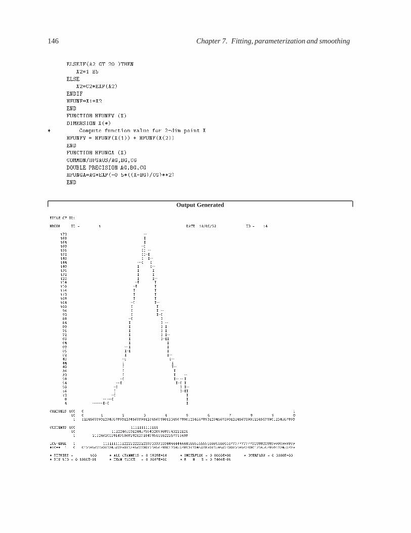
146 Chapter 7. Fitting, parameterization and smoothing
ELSEIF�A��GT�����THEN
X����E�
ELSE
X��C� EXP�A��
ENDIF
HFUNF�X��X�
END
FUNCTION HFUNFV �X�
DIMENSION X� �
Compute function value for ��dim point X
HFUNFV � HFUNF�X���� � HFUNF�X����
END
FUNCTION HFUNGA �X�
COMMON�HFGAUS�AGBGCG
DOUBLE PRECISION AGBGCG
HFUNGA�AG EXP����� ��X�BG��CG� ��
END
Output Generated
TITLE OF ID�
HBOOK ID � � DATE ��� ��� NO � ��
��� ��� I��� I�� I� � II � � III��� I I��� I I�� I I��� I I��� I I��� I I��� I I�� I I��� I I��� I I�� I I�� I I� I I�� I I �� I II�� I I�� I I � I I I�� I I I�� I I I�� I III�� I I� I I � II I � I I�� I I�� I I� I I�� I I�� I I �� I I I�� I II I� I I I�� I III�� I I� I I� II I
CHANNELS � �� � � � � � � � � � ���� �������� �������� �������� �������� �������� �������� �������� �������� �������� ����
CONTENTS � �������������� ������� ����� � �������� ���������� ��������������������������� �� ��� �������
LOWEDGE �� ���������������������������������������� �������������������������������������������� � ���� �������� �������� �������� �������� �������� �������� �������� �������� �������� ����
� ENTRIES � � � ALL CHANNELS � ���� E�� � UNDERFLOW � �E� � OVERFLOW � �E�� BIN WID � ��E� � MEAN VALUE � ����E� � R � M � S � �����E�

7.7. Fitting with finite Monte Carlo statistics 147
TITLE OF ID � �
HBOOK ID � � DATE ��� ��� NO � �
�� �� I� I I�� I I �� I I I I�� II I I I�� I I II I I� I I II I I �� I I III II�� I II II I�� I I I�� II I I� I I I I � I I I I � I I I I � I II I � I I I II II�� I I�� I I�� I I �� I I I� I I I�� I I I�� I I I�� I III�� I I� I I�� I I �� I I I I�� I I I I�� I I I I� II I II I �� III I I�� I II�� I I�� I I� I I� I I � I III� I I� I I
CHANNELS � �� � � � � � � � � � ���� �������� �������� �������� �������� �������� �������� �������� �������� �������� ����
CONTENTS � ������� ��� ���������������� ���������������� ��� ����� ������ ���� ������������ ��� ����� ��
LOWEDGE �� ���������������������������������������� �������������������������������������������� � ���� �������� �������� �������� �������� �������� �������� �������� �������� �������� ����
� ENTRIES � � � ALL CHANNELS � ���� E�� � UNDERFLOW � �E� � OVERFLOW � �E�� BIN WID � ��E� � MEAN VALUE � ����E� � R � M � S � ����E�

148 Chapter 7. Fitting, parameterization and smoothing
MINUIT RELEASE ���� INITIALIZED DIMENSIONS ���� �� EPSMAC� ���E��
����������
�� � ��SET EPS �����E��
����������
FLOATINGPOINT NUMBERS ASSUMED ACCURATE TO ����E��
����������������������������������������������
� �
� Function minimization by SUBROUTINE HFITH �
� Variablemetric method �
� ID � CHOPT � V �
� �
����������������������������������������������
Convergence when estimated distance to minimum �EDM� LT ���E�
PARAMETER DEFINITIONS�
NO NAME VALUE STEP SIZE LIMITS
� �P� � ����� ����� no limits
� �P� � ����� ����� no limits
�P � ������ ������ no limits
� �P� � ������ ������ no limits
� �P� � ������ � ����E�� no limits
� �P� � ������ � ����E�� no limits
����������
�� � ��SET PRINT �����
����������
����������
�� ��MIGRAD ���� ����
����������
MIGRAD MINIMIZATION HAS CONVERGED
MIGRAD WILL VERIFY CONVERGENCE AND ERROR MATRIX
FCN� ������� FROM MIGRAD STATUS�CONVERGED �� CALLS �� TOTAL
EDM� ���E�� STRATEGY� � ERROR MATRIX ACCURATE
EXT PARAMETER STEP FIRST
NO NAME VALUE ERROR SIZE DERIVATIVE
� P� ��� � ���� ������ ���� �E�
� P� ��� � ����� ������ ���� �E�
P � � �� ��� ��E�� ����� E� ���� �
� P� ������ ������E�� ����� E�� ��� �
� P� ������E�� ��� �E�� ������E� � ����
� P� ������ ��� ��E�� ������E� ��� ��
CHISQUARE � �����E��� NPFIT � ��
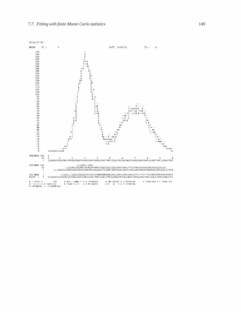
7.7. Fitting with finite Monte Carlo statistics 149
TITLE OF ID�
HBOOK ID � � DATE ��� ��� NO � ��
��� ��� I��� I�� I� � I���� � �II��� I I���� �I I�� I I���� � I��� I I���� I I��� �I I�� I I���� I I��� � I�� I I ��� I I� I I�� � I ��� I II�� I I�� � I � I I�I I I �� I I I I������ I�� �I I I I�� II I��I �� I I�I �� IIII��I�� I I I� I �� � I � I � I � � II I I�II I� � I I � I��� �I � I� I��� I I � I� � I � �� I ���� �I I �I II��� I � �I I��� �I I� I ��I I��� �I I���I�� I I �� I I �III II�� �� � II I���� ��I I��� �I I����� ������������I I�
CHANNELS � �� � � � � � � � � � ���� �������� �������� �������� �������� �������� �������� �������� �������� �������� ����
CONTENTS � �������������� ������� ����� � �������� ��������������� ��� ���������������� ���������������� ��������������������������� �� ��� ���������� ����� ������ ���� ������������ ��� ����� ��
LOWEDGE �� ���������������������������������������� �������������������������������������������� � ���� �������� �������� �������� �������� �������� �������� �������� �������� �������� ����
� ENTRIES � � � ALL CHANNELS � � E�� � UNDERFLOW � �E� � OVERFLOW � �E�� BIN WID � ��E� � MEAN VALUE � �����E� � R � M � S � �����E�� CHISQUAR � ��� �E��

150 Chapter 7. Fitting, parameterization and smoothing
����������������������������������������������
� �
� Function minimization by SUBROUTINE HFITV �
� Variablemetric method �
� ID � � CHOPT � V �
� �
����������������������������������������������
Convergence when estimated distance to minimum �EDM� LT ���E�
PARAMETER DEFINITIONS�
NO NAME VALUE STEP SIZE LIMITS
� �P� � ���� ������ no limits
� �P� � ����� � ���� no limits
�P � � ���� ������E�� no limits
� �P� � ������ ������ no limits
� �P� � ������E�� ������E�� no limits
� �P� � ������ � ����E�� no limits
����������
�� � ��SET PRINT �����
����������
����������
�� � ��MIGRAD ���� ����
����������
MACHINE ACCURACY LIMITS FURTHER IMPROVEMENT
MIGRAD MINIMIZATION HAS CONVERGED
MIGRAD WILL VERIFY CONVERGENCE AND ERROR MATRIX
EIGENVALUES OF SECONDDERIVATIVE MATRIX�
�����E��� �����E��� � ���E��� �����E��� �����E��� ��� �E���
MINUIT WARNING IN HESSE
�������������� MATRIX FORCED POSDEF BY ADDING ����� TO DIAGONAL
MIGRAD TERMINATED WITHOUT CONVERGENCE
FCN� ������� FROM MIGRAD STATUS�FAILED ��� CALLS ��� TOTAL
EDM� ���E��� STRATEGY� � ERR MATRIX NOT POSDEF
EXT PARAMETER APPROXIMATE STEP FIRST
NO NAME VALUE ERROR SIZE DERIVATIVE
� P� ����� �� �� E�� ������ �����
� P� ����� � �� �E�� ������ �����
P ������ ������E�� ������ �����
� P� ���� ������E�� ������ � ���
� P� ������E�� ������E�� ������ �� �
� P� ������ ��� � E�� ������ � � �
CHISQUARE � �����E��� NPFIT � ����
COVARIANCE MATRIX
�����������������
�� ��E��
�����E� �� ��E��
�����E�� �����E�� �����E��
�����E�� �����E�� �����E�� �����E��
�����E� �����E�� �� ��E�� �����E�� �����E��
�����E� � � �E�� �����E�� �����E�� �����E�� ���� E��
����������������������������������������������
� �
� Function minimization by SUBROUTINE HFITH �
� Variablemetric method �
� ID � � CHOPT � �
� �
����������������������������������������������

7.7. Fitting with finite Monte Carlo statistics 151
Convergence when estimated distance to minimum �EDM� LT ���E�
FCN� ������� FROM MIGRAD STATUS�CONVERGED �� CALLS �� TOTAL
EDM� � �E�� STRATEGY� � ERROR MATRIX ACCURATE
EXT PARAMETER STEP FIRST
NO NAME VALUE ERROR SIZE DERIVATIVE
� P� ��� � ���� ���� � �� ���E�
� P� � ���� ������E�� ������E�� �� ��
P ����� E�� ��� � E�� ������E� �����
CHISQUARE � �����E��� NPFIT � ��
EXAMPLE NO �
HBOOK ID � DATE ��� ��� NO � ��
�� �� I�� I I� ������ �� ��I I�I�� �I I I �I�� � II II��� �II I�� �I I��� I I��� �I I ��� �I I�I�� �I I� �I �� �I �� �I I�� �I I�� �I I � �I II�I� �I ��� �� I��� ��� I���� ����������������I I������������������������������������
CHANNELS � �� � � � � � � � � � ���� �������� �������� �������� �������� �������� �������� �������� �������� �������� ����
CONTENTS � ������������������������� � ������� �������� � ���������� ��������� �������� � ����������������� � ������������ ���� ��������� ������ �� �
LOWEDGE �� ���������������������������������������� �������������������������������������������� � ���� �������� �������� �������� �������� �������� �������� �������� �������� �������� ����
� ENTRIES � � ALL CHANNELS � � E�� � UNDERFLOW � �E� � OVERFLOW � �E�� BIN WID � ��E� � MEAN VALUE � �����E� � R � M � S � ���� E�� CHISQUAR � �����E��

152 Chapter 7. Fitting, parameterization and smoothing
Example of parametrization and smoothing
SUBROUTINE HEXAM�
������������
� PARAMETRIZATION � SMOOTHING
������������ � R�Brun �
DOUBLE PRECISION COEFF
DIMENSION ITERM����COEFF����
��������������������������������������������
Get hist ��� from data base
CALL HRGET�����hexam�dat�� ��
Find best parametrization of histogram in terms of powers
of shifted Tchebychev polynomials
also produces the corresponding fortran function �here on
standard output�
CALL HCOPY������ ��
CALL HSETPR��PNBX�����
CALL HSETPR��PNCX�����
CALL HSETPR��PLUN����
CALL HPARAM���������COEFFITERMNCO�
CALL HPRINT���
ID�� is smoothed with B�splines
statistical errors �sqrt of contents� are drawn
CALL HCOPY������ ��
CALL HSPLI������CHI��
CALL HIDOPT���ERRO��
CALL HPHIST���HIST���
END

7.7. Fitting with finite Monte Carlo statistics 153
Output Generated
����������������������������������������
� �
� MULTIDIMENSIONAL PARAMETRIZATION �
� �
����������������������������������������
FIT CHARACTERISTICS AND OPTIONS
�������������������������������
ID � �
DIM � �
WORKING SPACE IN �PAWC� � ����
� USERDEFINED BASIC FUNCTIONS
� USERDEFINED ELEMENTARY FUNCTIONS
MAX NUMBER OF REGRESSORS � ��
MAX POWERS OF POLYNOMIALS IN EACH DIM � ��
AMOUNT OF OUTPUT � �
WEIGHTING TYPE � �
CLASS OF POLYNOMIALS �
CLASS OF BASIC FUNCTIONS � �
BASIC FUNCTION SELECTION MODE � �
REGRESSION MODE � �
XNORMALIZATION TYPE � �
POWER LIMITOR � ���
FTEST LEVEL � ���
PARAMETRIZATION SUPERIMPOSED ON HISTOGRAM
FORTRAN CODE FPARAM WRITTEN ON UNIT �
FITTING PROCESS WILL STOP WHEN THE RESIDUAL VARIANCE HITS A MINIMUM
�� CANDIDATE BASIC FUNCTIONS WERE RETAINED FOR THE FIT
NUMBER OF POINTS TO FIT � ��
SUM OF SQUARES OF YVALUES � �����
MACHINE PRECISION � ���E��
FITTING PROCESS STOPPED AS RESIDUAL VARIANCE HITS MINIMUM
R� � ����� �� REGRESSORS INCLUDED
FINAL RESULTS OF THE FIT
������������������������
ITERATION RSS R�ADJ REGRESSOR COEFF VALUE TERM OF PARAMETRIZATION
� ����� ��� �� � �� �� �
� ���� ��
����� ��
� ����� ��
� ����� ���
� ����� ��
� ����� ���
� ����� ��
� ����� � �
�� �� �� ��
�� ���� ���
�� ���� �

154 Chapter 7. Fitting, parameterization and smoothing
����������������������������������������������������������
REGRESSOR STANDARD DEVIATION CONFIDENCE INTERVAL
� ������ � ���� � ����� �
� ����� � ��� � ���� �
������ � ����� � ���� �
� ����� � ��� � � ����� �
� ��� � � ���� � ����� �
� ����� � ����� � ����� �
� ������ � � ��� � ����� �
� ��� � � ����� � ��� � �
� ���� � � �� � ����� �
�� �� ��� � ���� � �� �� �
�� ������ � ��� � � ����� �
�� �� �� � ����� � ����� �
DOUBLE PRECISION FUNCTION FPARAM �X�
DOUBLE PRECISION COEFF�P�P��P��P��HELEFT�HBASFT
DIMENSION X����COEFF�����IBASFT� �����
DATA COEFF� ��� �����E����� �������E���� ���������E����
����������E���� ���������E�������������E����
����������E�������������E���� �������� E����
� ��� �����E����� ��� �� E���� � �������E���
��
DATA IBASFT� �� ��� ��� ������� ������� ���� �� ������� �
��
FPARAM��
DO �� K�����
P��
DO �� I��� �
NUM�IBASFT�I�K����
ITYP�IBASFT�I�K�NUM���
IF �NUMNE�� THEN
IF �ITYPEQ�� THEN
P���
P����X �I��
DO �� J���NUM
P�������X �I����P�P�
P��P�
�� P��P�
P�P�P�
END IF
IF �ITYPEQ�� P�P�HELEFT�NUM�X �I��
IF �ITYPEQ�� THEN
P�HBASFT�NUM�X �
GOTO ��
END IF
END IF
�� CONTINUE
�� FPARAM�FPARAM�COEFF�K��P
�� CONTINUE
RETURN
END

7.7. Fitting with finite Monte Carlo statistics 155
THIS HISTOGRAM IS FILLED ACCORDING TO THE FUNCTION HTFUN�
HBOOK ID � � DATE �������� NO � ��
��� ��� I��� I�� I� � II � � I��I��� � ���� �I ��� I I��� � ���� I I��� �I I���� I I�� I I���� � I��� I I�� I I ��� I I� � I�� I I ��� I II�� �I I�� I I� � I I I I I �� �I I I I�������� I�� I I � ��I II I �I �� I III �I IIII��I�� I I I� I �� � I � I�� I � � II I � II I� � I I� �I I��� �I I � I��� � I � �I I� � I I �I I �I�� � �I � �I I��� I I �I ���� �I I� I �I I��� � I I�I I �� I I ��� � ����III II ���� � � II I���� �I I�� � ���I I����� ������I I�
CHANNELS � �� � � � � � � � � � ���� �������� �������� �������� �������� �������� �������� �������� �������� �������� ����
CONTENTS � �������������� ������� ����� � �������� ��������������� ��� ���������������� ���������������� ��������������������������� �� ��� ���������� ����� ������ ���� ������������ ��� ����� ��
LOWEDGE �� ���������������������������������������� �������������������������������������������� � ���� �������� �������� �������� �������� �������� �������� �������� �������� �������� ����
� ENTRIES � � ALL CHANNELS � � E�� � UNDERFLOW � �E� � OVERFLOW � �E�� BIN WID � ��E� � MEAN VALUE � �����E� � R � M � S � �����E�� CHISQUAR � �����E��

156 Chapter 7. Fitting, parameterization and smoothing
THIS HISTOGRAM IS FILLED ACCORDING TO THE FUNCTION HTFUN�
HBOOK ID � � DATE �������� NO � ��
�� I�� I�� �� II I�� IIII�� IIII� III II� III��II�� � I�II�� I� I �I�� I�I III�� III �I�� I� ��� I I�� I�I I��� II I� �I� I� III� II I� I I� � II I I I I I� I I �I III I I� �I II II���II III� I� I I ����II���IIIII� � I I III��IIIII I��I� II � �II I II I I �� I� I � III�II I I II I �II �II I I�I I �� I I I� III� I I� I� �I I� I��I I � I� I I I�I II��� �I I� I I I �I � I� II �� I�� II I��II� I�I II�����II I�� I� �II I I II I I��� I�I I I ��� I �I I����I �������� II��
CHANNELS � �� � � � � � � � � � ���� �������� �������� �������� �������� �������� �������� �������� �������� �������� ����
CONTENTS � �������������� ������� ����� � �������� ��������������� ��� ���������������� ���������������� ��������������������������� �� ��� ���������� ����� ������ ���� ������������ ��� ����� ��
LOWEDGE �� ���������������������������������������� �������������������������������������������� � ���� �������� �������� �������� �������� �������� �������� �������� �������� �������� ����
� ENTRIES � � ALL CHANNELS � � E�� � UNDERFLOW � �E� � OVERFLOW � �E�� BIN WID � ��E� � MEAN VALUE � �����E� � R � M � S � �����E�� CHISQUAR � �����E��

Chapter 8: Memory Management and input/output Routines
8.1 Memory usage and ZEBRA
The hbook system uses the zebra data manager to store its data elements in a COMMON block �PAWC�(shared with the kuip and higz packages, when the latter are also used, as is the case in paw). In fact thefirst task of a hbook user is to declare the length of this common to zebra by a call to HLIMIT, as is seenin figures 1.2 and 1.4
In the �PAWC� data store, the hbook, higz and kuip packages have all their own division (see [10] formore details on the notion of divisions) as follows (see figure 8.1):
LINKS Some locations at the beginning of �PAWC� for zebra pointers.
WORKS Working space (or division �) used by the various packages storing information in �PAWC�
HBOOK Division � of the store. Reserved to hbook.
HIGZ A division reserved for the higz graphics package. This division only exists when higz iscalled.
KUIP A division reserved for the kuip user interface package. This division only exists when kuip iscalled.
SYSTEM The zebra system division. It contains some tables, as well as the Input/Outputbuffers for HRINand HROUT.
COMMON�PAWC�NWPAW�IXPAWC�IHDIV�IXHIGZ�IXKU�FENC���LMAIN�HCV���
DIMENSION IQ����Q����LQ������
EQUIVALENCE �LQ����LMAIN���IQ����LQ�����Q����IQ����
link
area
work
area
free
space
HBOOK
div
HIGZ
div
KUIP
div
system
div
Figure 8.1: The layout of the �PAWC� dynamic store
8.1.1 The use of ZEBRA
Inside the hbook division the various data elements are stored as a zebra data structure, one for each“identifier”. In fact all identifiers (histogram or Ntuple numbers) are stored in an ordered array in a zebrabank and access to the information associated with the hbook data is via the reference link at the sameoffset as the identifier in the data part of the bank. The data structure for a given element depends on itscharacteristics. In any case the top bank for a given element contains the title and other constants, whilethe data themselves are stored in another bank hanging from the previous one. Sometimes other banks are
157

158 Chapter 8. Memory Management and input/output Routines
created, e.g. for automatic binning, for storing the limits of the elements of a Ntuple and, when a Ntupleis kept in memory, for containing the overflow of the data, for projections, slices and bands in the 2-dimcase of for containing the errors associated to a bin. This means that each hbook identifier has a wholeset of attributes associated with its existence, and when a histogram or Ntuple is written to backup storeand later reread, the complete data structure, containing all characteristics and attributes are retrieved.Figure 8.2 shows the zebra data structure for a two-dimensional histogram. The precise layout of thisbank should be of no concern to the user. It is only shown here as an example of the underlying zebra
structure of hbook. Note the use of the data part of the bank for storing attributes (e.g. title, number ofbins, number of entries) as well as of the link part for storing the addresses to access the associated datapoints (scatter plot contents, X and Y projections, slices and bands and their associated errors).
8.2 Memory size control
CALL HLIMIT �NWPAW�
Action: Defines the maximum total size NWPAW of common �PAWC�.
Remark:
– HLIMIT must be called before any other hbook routine.
– hbook is compiled with a COMMON�PAWC� dimensioned to �����words. If NWPAW������, then thedefault value of ����� is assumed.
– If zebra has already been initialised, HLIMIT must be called with a negative argument, e.g. CALLHLIMIT��NWPAW�.
CALL HLOCAT �ID�LOC��
Action: Returns the pointer in common �PAWC� to the zebra ([10]) structure, which contains the de-scription of a given histogram.
Input parameter:
ID histogram identifier
Output Parameter:
LOC Pointer to the zebra bank containing the histogram information.
This routine can be useful to access directly the memory area of a given histogram, to extract any infor-mation that cannot be obtained with the entries previously described.
8.2.1 Space requirements
The argument NWPAWCmust be given a value large enough to accomodate in memory all histograms (1-Dand 2-D) and all Ntuple headers and buffers, i.e.
NWPAWC � ����� �NFXi��
SF �i� �N�Xi��
S��i� �N�Xi��
S��i� �NTXi��
SN �i�

8.2. Memory size control 159
Figure 8.2: The zebra data structure used for two-dimensional histograms
ZEBRA structure for HBOOK tables
LCID (pointer to histogram/table ID)
Histogram attributes, parameters, title-1-2-3-4-5-6-7
LSCAT
Sum of contents for 2-D (NX*NY)
LPROXContents PROX Errors PROX
LPROYContents PROY Errors PROY
LSXI
LSLIX
-1-I-NSX
Contents SLIX I Errors SLIX ILSLIY
same as LSLIX
-1 -1
LBANX
BANX 1 BANX 2
Contents BANX 1 Errors BANX 1
LBANYsame as LBANX

160 Chapter 8. Memory Management and input/output Routines
NF Number of open files
SF �i� 100+LRECi, where LREC is the buffer size for file i, as specified in a call to HROPEN.
N� Number of 1-D histograms
S��i� Space occupied by 1-D histogram i, i.e.����NCHAN����PACK�IERR��NCHAN�����IFUN��NCHAN����
NCHAN Number of channels in histogram
PACK Packing factor (1. by default). See parameter VMX of HBOOK�.
IERR � if HBARX called, � otherwise.
IFUN � if the histogram has an associated function (HFUNC, fits or smoothing)
N� Number of 2-D histograms
S��i� Space occupied by 2-D histogram i, i.e.����NCHANX�����NCHANY����PACK + space for projections, slices and bands (which are 1-Dhistograms).
NT Number of Ntuples
S��i� Space occupied by headers and buffers of Ntuple i (see routines HBOOKN and HBNT).
8.3 Directories
hbook histogram data are kept in a zebra tree structure similar to the directory structure of the Unix filesystem. Note that the zebra RZ package uses the same conventions. (In fact, hbook uses the zebra
RZ package to manage files). With this convention, all references to histograms are still made using aninteger identifier, but this identifier is relative to a directory. hbook initially sets the current directory tobe ��PAWC. This directory remains the current directory until changed either explicitly or implicitly byone of the calls described below. As with the Unix file system the current directory can be a subdirectory,e.g. ��PAWC�L�, ��PAWC�L��L�� and ��PAWC�L��L��.
These hbook directories can reside in the local memory of the computer (i.e. the PAWC common, or theycan be stored on a local (��LUN�) or remote disk file system (��VXCRNA). They can even be dynamicallycreated by a “producer” in the memory of a remote computer and ”shared” by that machine with the user’smachine via global section (VMS) or shared memory (Unix).
HMDIR HCDIR HLDIR HDDIR HPDIR
�������� ��PAWC local memory X X X X X
! ! ��LUN� local disk X X X X X
! USER ! ��VXCRNA ���� telnet �rsh� remote disk X X X
! ! ��GLOSEC ���� tcp�ip ��� global section�VMS� X X X
�������� ��SHARE ���� tcp�ip ��� shared memory�Unix� X X X
Figure 8.3: Different kinds of hbook directories
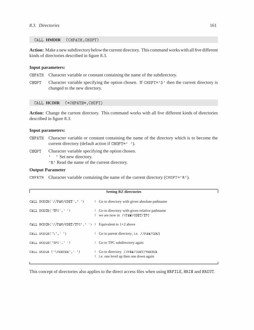
8.3. Directories 161
CALL HMDIR �CHPATH�CHOPT�
Action: Make a new subdirectorybelow the current directory. This command works with all five differentkinds of directories described in figure 8.3.
Input parameters:
CHPATH Character variable or constant containing the name of the subdirectory.
CHOPT Character variable specifying the option chosen. If CHOPT��S� then the current directory ischanged to the new directory.
CALL HCDIR ��CHPATH��CHOPT�
Action: Change the current directory. This command works with all five different kinds of directoriesdescribed in figure 8.3.
Input parameters:
CHPATH Character variable or constant containing the name of the directory which is to become thecurrent directory (default action if CHOPT�� �).
CHOPT Character variable specifying the option chosen.� � Set new directory.�R� Read the name of the current directory.
Output Parameter
CHPATH Character variable containing the name of the current directory (CHOPT��R�).
Setting RZ directories
CALL HCDIR����PAW�CDET�� �� � Go to directory with given absolute pathname
CALL HCDIR��TPC�� �� � Go to directory with given relative pathname� we are now in ��PAW�CDET�TPC
CALL HCDIR����PAW�CDET�TPC�� �� � Equivalent to 1+2 above
CALL HCDIR����� �� � Go to parent directory, i.e. ��PAW�CDET
CALL HCDIR��TPC�� �� � Go to TPC subdirectory again
CALL HCDIR ���VERTEX�� �� � Go to directory ��PAW�CDET�VERTEX
� i.e. one level up then one down again
This concept of directories also applies to the direct access files when using HRFILE, HRIN and HROUT.

162 Chapter 8. Memory Management and input/output Routines
CALL HLDIR �CHPATH�CHOPT�
Action: List the contents (identifiers, type of histograms and titles) of a hbook directory. This commandworks with all five different kinds of directories described in figure 8.3.
Input parameters:
CHPATH Character variable or constant containing the name of the directory to be listed. CHPATH�� �
stands for the current directory.
CHOPT Character variable specifying the chosen option.
� � List only the top directory.
�A� List all Ntuple extentions.
�I� HINDEX option selected instead of simple list.
�N� List only the Ntuples.
�R� List using RZ format.�S� Sort the directory entries.
�T� List the complete subdirectory tree starting from the specified directory.
List all existing directories in //PAWC
CALL HLDIR ����PAWC��T��
CALL HDDIR �CHPATH��
Action: Delete a (sub)directory from memory or local disk.
Input parameter:
CHPATH Character variable or constant specifying the pathname of the (sub)directory to delete.CHPATH�� � stands for the current directory.
CALL HPDIR �CHPATH�CHOPT�
Action: Print the contents of a directory (This routine calls HPRINT). This routine works only for direc-tories in local memory or remote RZ files accessed opened via XZRZOP (see the CSPACK manual [19] formore information).
Input parameters:
CHPATH Character variable or constant specifying the pathname of the directory to be printed.CHPATH�� � stands for the current directory.
CHOPT Character variable specifying the option chosen.
� � Print the contents of the top directory.
�I� Print an index.
�T� Print the complete directory tree (i.e. the top directory and its subdirectories).

8.3. Directories 163
Printing list of histograms
CALL HPDIR ����PAWC��T�� � Print list of all histograms in ��PAWC
CALL HPDIR �� �� �� � Print list of all histograms in current directory
CALL HPRINT��� � Print histograms in current directory
CALL HLNEXT ��IDH��CHTYPE��CHTITL��CHOPT�
Action: Scan the contents of the current directory in memory or on an RZ file.
Input parameters
IDH Must be zero for first call
CHTYPE Character variable specifying items to be scanned.
��� include 1-D histograms
��� include 2-D histograms
�N� include Ntuples
�D� include subdirectories
� � include everything, i.e., equivalent to ���ND�.
Output parameters
IDH On return contains identifier of next histogram. When all histograms are processed, a value ofzero is returned.
CHTYPE Character variable specifying type of histogram.
��� 1-dimensional
��� 2-dimensional
�N� Ntuple
�D� subdirectory
��� unknown.
CHTYPE Character variable containing title or subdirectory name.
Scan content of current directory
IDH��
� CONTINUE
CALL HLNEXT�IDHCHTYPECHTITLCHOPT�
IF�IDH�NE��� THEN
��� process
GOTO �
ENDIF

164 Chapter 8. Memory Management and input/output Routines
CALL HRDIR �MAXDIR�CHDIR��NDIR��
Action: Returns the list of subdirectories of the current working directory. This command works with allfive different kinds of directories described in figure 8.3.
Input parameter
MAXDIR Length of the character array CHPATH.
Output parameters
CHDIR� Character array which will contain the names of the subdirectories of the current working di-rectory.
NDIR� Actual number of subdirectories present in the current working directory. If this number isgreater than MAXDIR, only the first MAXDIR subdirectory names will be returned in array CHDIR.
The use of directories is illustrated below:
Example of use of directories
PROGRAM MAIN
COMMON�PAWC�H�������
CALL HLIMIT �������
CALL HBOOK� ����Energy distribution������������
" "
CALL USECAL
" "
CALL HFILL ���EDER�����
" "
CALL HISTDO
" "
END
SUBROUTINE USECAL
Make a new directory ECAL and set the new current directory
CALL HMDIR ��ECAL��S��
Create a new histogram with ID��� in the new directory
CALL HBOOK� ����My histogram�����������
" "
CALL HFILL ���UX����
" "
Go back to the parent directory
CALL HCDIR ����� ��
" "
END

8.4. Input/Output Routines 165
8.4 Input/Output Routines
hbook files are in fact zebra RZ files [10]. Input/output error return codes are available vin the zebracommunication vector IQUEST, and the user should consult the RZ manual for their meaning. Both diskand memory resident files are supported, the latter being particularly useful in online applications, wherehistogram data have to be shared between different processes.
hbook files are written in Zebra exchange format and thus need not be converted when transferred be-tween different computer systems using binary ftp (see section 8.5), or accessed over the network usinga distributed file system such as AFS or NFS.
Reading and writing histograms to a direct access file
CALL HRPUT �ID�CHFILE�CHOPT�
Action: Write a histogram to a given direct access file. This routine cannot be used for Ntuples.
Input parameters:
ID Histogram identifier. ID�� writes all histograms in the current directory to the output file.
CHFILE Character variable or constant defining the filename.If CHFILE�� � the histogram is saved in the current working directory on disk.
CHOPT Character option specifying the desired option.
�N� Write the histogram to a New file.
�T� Can be used together with ID��. All histograms in the current directory and all subdi-rectories in memory are written to the output file.
�U� Write the histogram to an already existinghbook file. When an histogram with the sameidentifier already exists on the output file, then a new cycle is added.
CALL HRGET �ID�CHFILE�CHOPT�
Action: Read a histogram from a given direct access file. This routine cannot be used for Ntuples.
Input parameters:
ID Histogram identifier. ID�� read all histograms into the current directory.
CHFILE Character variable or constant defining the input filename.If CHFILE�� � the histogram is read from the current working directory on disk.
CHOPT Character option specifying the desired option.
�A� Add to the current histogram in memory.
�T� Get a complete tree (not yet implemented)
Remarks:
The following remarks apply to both HRPUT and HRGET.

166 Chapter 8. Memory Management and input/output Routines
– HRGET and HRPUT issue automatically Fortran OPEN and CLOSE calls.
– With HRPUT the file is created with LREC����� machine words.
– On VM/CMS no FILEDEF statement should be given. The filename CHFILE can be given in eitherof the forms Filename Filetype Filemode or Filename�Filetype�Filemode
– On Unix the filename CHFILE will be translated to lowercase.
– Fortran logical unit 88 is used by these routines.
– HRPUT calls HROPEN, HROUT and HREND.
– HRGET calls HROPEN, HRIN and HREND.
Open an RZ direct access file or map a Global Section
CALL HROPEN �LUN�CHTOP�CHFILE�CHOPT��LREC��ISTAT��
Action: Open a direct access hbook file. If several direct access files are opened, they are identified bythe top directory only.
Input parameters:
LUN Logical unit number associated to the file.
CHTOP Character variable specifying the name of the top directory associated withunitLUN (maximum8 characters). This is an arbitrary name used to identify the file on unit LUN in subsequent callsto HR�� routines.
CHFILE Character variable specifying the name of the file to be opened.
CHOPT Character variable specifying the options selected
Medium� � Disk (default)
�G� Global Section (see chapter 9)
mode � � Existing HBOOK file (default)
�N� Create a new file
�Q� Override default number of records for new file with contents of IQUEST����
�X� The file is/will be in exchange format
�U� Update an existing file
LREC Record length in machine words (recommended value is 1024). If LREC�� the actual recordlength is returned on exit.
Output parameters:
ISTAT Return code. ISTAT�� indicates success.
LREC (Only when �LREC=0) on input) The actual record length of the file on disk.
Remarks:
– HROPEN performs a Fortran direct access open for the file CHFILE on logical unit LUN.
– On VM/CMS no FILEDEF statement should be given. The filename CHFILE can be given in eitherof the forms Filename Filetype Filemode or Filename�Filetype�Filemode

8.4. Input/Output Routines 167
– On Unix the filename CHFILE will be translated to lowercase.
– If LREC�� on input, HROPEN will automatically determine the record length of existing files.
– On MVS systems, the current userid prefix will be automatically added to the front of the file nameunless the first character is a dot (.).
– The maximum number of records is by default 32000. You can use option �Q� to change this.
– A file declared with HROPEN must be released with HREND.
– HROPEN calls HRFILE internally.
CALL HRFILE �LUN�CHTOP�CHOPT�
Action: Establishes a temporary unique correspondance between a logical unit and a top directory name.Users should call HROPEN instead of HRFILE.
By default, HROPEN (HRFILE) creates new files (option N) with the maximum number of records set to alarge number (default 32000). If this is insufficient, the user can override this value by specifying the Qoption and setting IQUEST���� to the actual number of records required (up to a maximum of 65K).
Overriding the default record allocation
COMMON�QUEST�IQUEST����� � Declare IQUEST communication vector
IQUEST���� � ����� � I require ����� records
CALL HROPEN���FILE��file�ext��NQ�����ISTAT� � Call HROPEN
Note that after a call to HROPEN (HRFILE) (if CHTOP��MYDST� for example), the current directory is setto ��MYDST. If LUN is an existing file, one can change the current directory to an existing subdirectory,SUBDIR, using CALL HCDIR ��SUBDIR��� ��, setting the current directory CD to ��CHTOP�SUBDIR.
– The contents of a directory is listed using routine HLDIR.
– A new subdirectory can be created with routine HMDIR.
– The current directory in memory (��PAWC�) and hence on the direct access files may be set byone of the routines HCDIR or HMDIR.
Note that when calling HCDIR or HRFILE on a direct access file, the current directory in memory will bethe latest current directory set.
Writing to a file
CALL HROUT �ID�ICYCLE��CHOPT�
Action: Write a histogram from the current directory in memory onto the current directory on the directaccess file.
Input parameters:
ID Histogram identifier. ID�� means write all histograms from the current directory in memory.
CHOPT Character variable specifying the options selected.
�N� Create on the direct access file the same directory tree as in memory.

168 Chapter 8. Memory Management and input/output Routines
�T� Write the whole directory tree hanging from the current directory (if ID��).
Output parameter:
ICYCLE Cycle number. The first time a given histogram with identifier ID is stored on a directory on adirect access file, ICYCLE is set to �. If the histogram identifier ID already exists on the directaccess file, then the call to HROUT will increment the cycle number ICYCLE by one.
Experienced users may invoke routines from the zebra RZ package to purge a directory, i.e. delete allversions of an identifier but the most recent one using routine RZPURG.
Reading from a direct-access file or global section
CALL HRIN �ID�ICYCLE�IOFSET�
Action: Read a histogram from the current directory on the direct access file (or global section) into thecurrent directory in memory.
Input parameters:
ID Histogram identifier. ID�� means that all histograms from the current directory on the directaccess file (global section) should be read into memory. If a histogram identifier ID alreadyexists in memory a message is printed and it is deleted from memory before reading the newhistogram from the file or global section.
ICYCLE Cycle number. If ICYCLE�� then the lowest cycle is read. To read the highest cycle, use a largenumber, e.g. 999999.
IOFSET The histogram which is read in memory will have the identifier IDN�ID�IOFSET. SpecifyingIOFSET different of zero permits to have in memory copies of histograms with the same iden-tifiers ID in different files. This parameter may be very useful when HRIN is called togetherwith routines such as HOPERA or HDIFF. This facility also works for Ntuples.
Merging HBOOK files into a new file
CALL HMERGE �NFILES�CHFIN�CHFOUT�
Action: Merges two or more HBOOK files with identical objects and directories into a new file. His-tograms are added and Ntuples are combined. Works for CWN’s and RWN’s.
Input parameters:
NFILES Number of input files to be merged.
CHFIN Character array (e.g., CHARACTER�� CHFIN���� for 10 files whose names are not longer than8 characters) containing the name(s) of the file(s) to be merged.
CHFOUT Character variable with the name of the output file.
CALL HMERGIN
Action: Identical to HMERGE but the routine prompts interactively for the names of the input and outputfiles. The paw command NTUPLE�HMERGE calls this routine.

8.4. Input/Output Routines 169
Scratching histogram in a file
CALL HSCR �ID�ICYCLE�CHOPT�
Action: Scratch (delete) a histogram from the current directory in the direct access file.
Input parameters:
ID Histogram identifier. ID�� means scratch all histograms in the current directory.
ICYCLE Cycle number. If ICYCLE�� then all cycles are deleted.
CHOPT Character variable specifying options selected.
� � Only possible value (not used at present)
Close a file
CALL HREND �CHTOP�
Action: Closes a direct access file if is not needed anymore or when the options �N� or �U� are specifiedin HRFILE.
Input parameter:
CHTOP Character variable specifying the name of the top directory associated with the file to be closed.This should correspond to the name declared with HRFILE. After this call, the system bank as-sociated to this file is deleted. The call to HREND is obligatory when the file has been modified.
Remark:
A Fortran CLOSE statement should follow a call to HREND.

170 Chapter 8. Memory Management and input/output Routines
8.5 Exchange of histograms between different machines
hbook files are by default created in exchange mode. They can be transported between machines usingthe standard binary FTP or they can be NFS mounted in a heterogeneous environment.
Transfer between Unix machines with FTP
� ftp remote
ftp� bin
ftp� get remote�hbook
Transfer from CERNVM to a Unix workstation
On CERNVM type the following:
CMS FTP workstation
ftp� BIN F ���� � block size in bytes
ftp� PUT file�hbook
Running FTP on a VAX/VMS systen
� ftp remote
ftp� bin
ftp� get remote�hbook
ftp� quit
� resize �s ���� remote�hbook#�
The resize command does not copy the file. It simply changes the header information, from 512 byterecords to 4096 bytes. In case the block size of the hbook file is not 1024 words (LREC parameter ofroutine HROPEN), i.e. 4096 bytes, specify the corresponding value as parameter to the resize command.
The resize tool is available on request from the CERN Program Library.
Proposed hbook file naming convention
Users are encouraged to name their hbook files with the suffix �hbook, so that the paw�� browserwill be able to recognize these files automatically.

8.6. RZ directories and HBOOK files 171
8.6 RZ directories and HBOOK files
Another advantage of the use of zebra in hbook is that zebra’s direct access RZ package is available.The RZ package allows data structures to be uniquelyaddressed via pathnames, which are based on Unixfile names. Related data structures are addressed from a directory.
Routine HROPEN issues a the Fortran OPEN statement and declares the RZ top directory.
Example of using HROPEN
CALL HROPEN�LUN�HISTO���HISTOS�DAT�CHOPTLRECLISTAT�
In this example, HROPEN issues a Fortran direct-access open statement for the file HISTOS�DAT. If, oninput, LRECL contains the value 0, HROPENwill automatically determine the record length of the file, pro-vided that the file already exists.
Each time a RZ file is opened via a call to HROPEN or HRFILE, a supplementary top directory is createdwith a name specified in the calling sequence. This means that the user can more easily keep track of hisdata and also the same histogram identifiers can be used in various files, what makes life easier if onewants to study various data samples with the same program, since they can be addressed by changing tothe relevant file by a call to HCDIR first. For more information on the RZ package, see the zebra RZmanual.
In the case of the second call to HROPEN, where update mode is requested, it is the users responsibility toensure that write-acess is enabled, i.e. the file is not on a read-only mini-disk (VM/CMS systems), or isopened with the SHARED attribute (VAX/VMS systems) etc.
A Fortran CLOSE statement is also required for each file after calling HREND. Further details of hbook’susage of zebra RZ files are given below.
Defining hbook files
CALL HROPEN���HISTO���HISTO��DAT�� �����ISTAT� � Open first HBOOK RZ file �read only�
CALL HROPEN���HISTO���HISTO��DAT��U�����ISTAT� � Open second HBOOK RZ file �update�
CALL HCDIR����HISTO��� �� � Make HISTO� current directory
CALL HRIN��������� � Read ID �� on file �
����
CALL HCDIR����HISTO��� �� � Make HISTO� current directory
CALL HRIN��������� � Read ID �� on file �
����
CALL HROUT���ICYCLE� �� � Write ID �� to file �
CALL HREND��HISTO��� � Close file �
CALL HREND��HISTO��� � Close file �
In the previous example (and also in figures 1.2 and 1.4) it is shown how an external file is available viaa directory name inside hbook (and paw), and that one can change from one to the other file by merelychanging directory, with hbook routine HCDIR

172 Chapter 8. Memory Management and input/output Routines
Using subdirectories
The use of subdirectories, both in memory and on disk, is shown in the following examples.
Example of using subdirectories
PROGRAM TEST
INTEGER NWPAWC
PARAMETER �NWPAWC�������
COMMON�PAWC�PAW�NWPAWC�
CHARACTER � CHTAGS���
DIMENSION EVENT���
EQUIVALENCE �EVENT���X��EVENT���Y��EVENT��Z�
EQUIVALENCE �EVENT���ENERGY��EVENT���ELOSS�
DATA CHTAGS��X��Y��Z��Energy��Eloss��
�� Tell HBOOK how many words are in PAWC�
CALL HLIMIT�NWPAWC�
CALL HROPEN���EXAMPLE��EXAMPLE�DAT��N�����ISTAT�
IF�ISTAT�NE���GO TO ��
�� Make sub�directory on disk �as HROUT does not do this for us��
CALL HMDIR ��US��S��
CALL HCDIR����PAWC�� ��
�� Make sub�directory in memory�
CALL HMDIR ��US��S��
CALL HCDIR����PAWC�US�� ��
�� Book Ntuple � �d histogram
CALL HBOOKN����A simple Ntuple���EXAMPLE�����CHTAGS�
CALL HBOOK������Energy distribution�������������
�� Fill the Ntuple and histogram
DO �� I������
CALL RANNOR�XY�
Z�SQRT�X X�Y Y�
ENERGY���� � ��� X
ELOSS���� ABS�Y�
CALL HFN���EVENT�
CALL HFILL����ENERGY�����
�� CONTINUE
�� Juggle top directories �order of these calls is important����
CALL HCDIR����PAWC�� ��
CALL HCDIR����EXAMPLE�� ��
�� Write out everything to disk
CALL HROUT��ICYCLE�T��
�� Flush remaining buffers to disk�
CALL HREND��EXAMPLE��
�� CONTINUE
END

Chapter 9: Global sections and shared memory
9.1 Sharing histograms in memory on remote machines
When HBOOK is used in a data acquisition system environment, global sections can be an interestingalternative to disk input/output. The following example is a simple illustration of this facility.
Let us assume two processes exist:
1 PFILL, the process filling some histograms in COMMON�PAWC� directly.
2 PRESENT, a process activated from time to time to visualize the histograms created and filled byPFILL.
No hand-shaking mechanism is required. A global section is created (this is system dependent). Thisglobal section is mapped to COMMON�PAWC� in process PFILL and to COMMON�PAWMAP�PAWM�nwords�
in PRESENT. This process has also a COMMON�PAWC�, which will be used as a working space common.
A call CALL HRFILE �PAWM��PFILL���GN�� in process PRESENT will open a HBOOK global section.The current directory is now set to ��PFILL. RoutineHCDIRmay be used to change the current directoryto lower level directories. Using HRIN (described below) a histogram can now be copied from PFILL to�PAWC� of process PRESENT and invoke the printing or plotting routines of either HBOOK or HPLOT.
Tools exist (for example in PAW) to dynamically map global sections. It should be noted however that thismechanism does not allow to write (e.g. using routine HROUT) from process PRESENT into PFILL.
It is possible to open more than one global section (several processes PFILL).
9.1.1 Memory communication
CALL HCOPYM �ID�IPAWD�IOFSET�
Action: Copies one or more histograms from the PAW area to common �PAWC�.
Input parameters:
ID Identifier of the histogram. ID�� means copy all existing histograms.
IPAWD PAW area identifier.
IOFSET Offset of newly created histogram(s), i.e. new histogram(s)will have identifier(s)ID�IOFSET.
9.2 Mapping global sections on VMS
VALUE � hcreateg �global�name�base�common�size�
Action: Function to create and map a global section .
The function first opens a file with UFO option (using HST�OPEN�GBL), then creates and maps the globalsection using SYS�CRMPSC. Open the file using SYS�SETDFPROT to set protection loose.
Input parameters:
global�name Name of the section to be mapped
173

174 Chapter 9. Global sections and shared memory
base�common First word of COMMON to be mapped.
size size of the COMMON in words.
The function value returned is equal to the global section length (pages) if the procedure was successfulor an errorcode �� if an error occurred.
HCREATEG�DIR is a LOGICAL which, if defined, gives the directory for the mapping file of the globalsection. In this case, the file is not deleted upon closing.
VALUE � hmapg �global�name�base�common�offset�
Action: Function to dynamically map to an existing global section.
The function maps to the global section using SYS�MGBLSC, allocating pages in the p� region with thesec�m�expreg option.
Input parameters:
global�name Name of the section to be mapped
base�common First word of reference COMMON to be mapped.
offset Offset with respect to BASE�COMMON of the mapped section in words,i.e. BASE�COMMON�OFFSET� is the first word.
The function value returned is equal to the global section length (pages) if the procedure was successfulor is an errorcode �� if an error occurred.
VALUE � hfree �global�size�base�common�offset�
Action: Function to dynamically delete/unmap global section space using the service SYS�DELTVA.
Input parameters:
global�size Size of the section to be freed (pages).
base�common First word of reference COMMON.
offset Offset with respect to BASE�COMMON of the mapped section in words,i.e. BASE�COMMON�OFFSET� is the first word.
The function value returned is equal to the global section length (pages) if the procedure was successfulor is an errorcode �� if an error occurred.

9.2. Mapping global sections on VMS 175
9.2.1 Using PAW as a presenter on VMS systems (global section)
PROGRAM PRODUCE
PARAMETER MAXPAGES����
COMMON�PAWC�IPAWC���� MAXPAGES�
CHARACTER � GNAME
INTEGER � HCREATEG
GNAME��GTEST�
WAIT�TIME���
NUMEVT�����
�������������� Create Global section
NPAGES�HCREATEG�GNAMEIPAWC��� MAXPAGES�
IF�NPAGES�GT��� THEN
PRINT ����GNAME
���� FORMAT�� Global Section� �A� created��
ELSE
IERROR��NPAGES
PRINT ����IERROR
���� FORMAT�� Global Section Error� I��
GO TO ��
ENDIF
CALL HLIMIT���� NPAGES�
��������������� Book histos�
CALL HBOOK�����Test�������������
CALL HBOOK�����Test�������������
��������������� Fill histos�
DO �� I��NUMEVT
DO �� J�����
CALL RANNOR�AB�
CALL HFILL���A�����
CALL HFILL���B�����
�� CONTINUE
CALL LIB�WAIT�WAIT�TIME�
�� CONTINUE
�� STOP
END
� fort produce
� link produceSYS�INPUT�OPTIONS�
cern�library�packlib�libkernlib�lib
PSECT�PAWCPAGE
PAW � edit produce
macro produce ntimes����
nt��ntimes�
zone � �
histo�plot �� K
histo�plot �� K
loop�
histo�plot �� U
histo�plot �� U
wait � � �
nt��nt� ��
if nt�� goto loop
return
PAW � global�sect GTEST
PAW � exec produce ntimes���
Test1
0
40
80
120
160
200
240
280
320
-4 -3 -2 -1 0 1 2 3 4
Test2
0
40
80
120
160
200
240
280
-4 -3 -2 -1 0 1 2 3 4
Figure 9.1: Visualise histograms in global section
In addition to the facilities described in the previous section, the standard version of PAW may be usedas an online presenter on VMS systems using the mechanism of global sections. It is possible for twoprocesses to reference the same histograms using global sections. For example, the first process may bea histogram producer (e.g. a monitoring task) and the second process PAW. As the histograms are beinggradually filled by the first task, PAW can view them, and even reset them. To use the global sections,it is also necessary to ”page align” the common which is in the global section. This is achieved in the”link step” when making the process (see example). The relevant statements are SYS�INPUT�OPTIONSto tell the linker that some options follow the link statement, and PSECT�PAWC�PAGEwhich is the optionto page align the �PAWC� common.
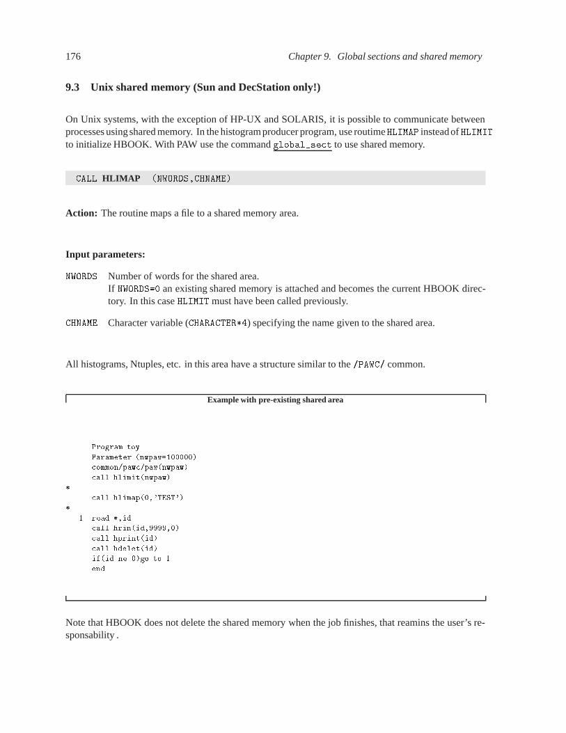
176 Chapter 9. Global sections and shared memory
9.3 Unix shared memory (Sun and DecStation only!)
On Unix systems, with the exception of HP-UX and SOLARIS, it is possible to communicate betweenprocesses using shared memory. In the histogramproducer program, use routimeHLIMAP insteadof HLIMITto initialize HBOOK. With PAW use the command global�sect to use shared memory.
CALL HLIMAP �NWORDS�CHNAME�
Action: The routine maps a file to a shared memory area.
Input parameters:
NWORDS Number of words for the shared area.If NWORDS�� an existing shared memory is attached and becomes the current HBOOK direc-tory. In this case HLIMIT must have been called previously.
CHNAME Character variable (CHARACTER��) specifying the name given to the shared area.
All histograms, Ntuples, etc. in this area have a structure similar to the �PAWC� common.
Example with pre-existing shared area
Program toy
Parameter �nwpaw��������
common�pawc�paw�nwpaw�
call hlimit�nwpaw�
call hlimap���TEST��
� read id
call hrin�id������
call hprint�id�
call hdelet�id�
if�id�ne���go to �
end
Note that HBOOK does not delete the shared memory when the job finishes, that reamins the user’s re-sponsability .

9.3. Unix shared memory (Sun and DecStation only!) 177
9.3.1 Using PAW and Unix shared memory (Sun and DecStation only)
Program hserver
HBOOK program creating a "shared memory"
area called �TEST�
Routine HLIMAP replaces HLIMIT�
NWORDS is the amount of space requested
in the shared area�
parameter�nwords�������
call hlimap�nwords�TEST��
call hbook����test�����������
call hcopy����test���
call hcopy���test��
do �� i�����������
call rannor�ab�
call hf���a���
call hf���b���
call hf��a ��b ����
if�mod�i��������eq���
X print � hserver in loop index �i
�� continue
end
� f�� �L��� �l��� �ohserver hserver�f
� hserver
GLOBAL MEMORY CREATED
offset from LQ � ���������
hserver in loop index ������
hserver in loop index ������
hserver in loop index �����
hserver in loop index ������
hserver in loop index ������
hserver in loop index ������
hserver in loop index ������
PAW � edit shared
macro shared ntimes����
histo�plot � K
do nt � ��ntimes�
histo�plot � U
wait � � �
enddo
return
PAW � global�sect TEST
PAW � exec shared ntimes���
Figure 9.2: Visualise histograms in Unix sharedmemory
On Unix PAW can be used as an online presenter using the shared memory facility (at present on Sunand DecStation only) and the routines described in section 9.3 Figure 9.2 shows on the left hand side theprogram, which fills the histograms. It is compiled and linked with the f�� command, and then started.It writes the lines shown while going through the event loop. Then PAW is started, communication isestablished via the command global�sect TEST, which declares that the area called �MAP� is to beshared for data communication, and the execution of the KUMAC program shared�kumac, shown atthe top right of the figure, is initiated.
The output shown on the screen then allows one to follow interactively (using the Update option �U� ofthe plot command) how the event generator (the hserver program) fills histogram number one. The firstfifteen iterations have been captured and are shown at the bottom right of Fig. 9.2.

178 Chapter 9. Global sections and shared memory
9.4 Access to remote files from a PAW session
When running PAW, it is often necessary to access files (e.g. HBOOK files) which reside on a differentcomputer. Therefore a PAW server is provided, which works using a conventional Client/Server model.The client (PAW) typically runs on a workstation. When the PAW command RLOGIN is invoked, a PAWserver is automatically started on the remote machine, normally a mainframe or data server.
Once the RLOGIN REMOTE command has been executed, the PAW Current Directory is set to ��REMOTE.The PAW client can now instruct the PAW server to attach a file using the RSHELL command (e.g. rshellfile pawtest�dat). If an histogram with HBOOK ID=10 is on the remote file, than the PAW commandHisto�Plot ��will plot this histogram on the local workstation. The histogram resides on ��PAWC likeother histograms coming from local files.
The RSHELL command may be used to communicate with the PAW server. The expression typed fol-lowing RSHELL is passed to the server. The current implementation of the PAW server recognizes thecommands:
rshell file filename Server connects filename
rshell cdir ��lun�� Server changes current directory
rshell ld Server lists current directory
rshell ld �� Server lists all connected files
rshell message Server pass message to operating system
Access to remote files from a workstation
PAW � rlogin CERNVM ! connect to CERNVM
PAW � rshell file HRZTEST�HBOOK ! PAW server connects HRZTEST HBOOK A to ��LUN��
PAW � histo�plot �� ! plot histogram �� from CERNVM
PAW � histo�fit �� G ! fit histo �� with a gaussian and plot it
PAW � rlogin VXCRNA ! connect to VXCRNA
PAW � rshell file DISK�DL��PAW�HEXAM�DAT# ! PAW server on VXCRNA connects file to ��LUN��
PAW � histo�plot ��� ! plot histogram ��� from VXCRNA
PAW � rshell file HRZTEST�DAT ! PAW server on VXCRNA connects file to ��LUN��
PAW � histo�plot ��� s ! plot histogram ��� from HRZTEST�DAT
! on VXCRNA on the existing picture
PAW � rshell ld �� ! list all files connected on VXCRNA
PAW � cdir ��CERNVM ! Change current PAW directory to CERNVM
PAW � histo�plot ��� ! plot histogram ��� from CERNVM
PAW � histo�plot ��VXCRNA���� ! plot histogram ��� from VXCRNA
PAW � cdir ��PAWC ! current directory to local memory
PAW � histo�list ! list all histograms in ��PAWC
PAW � Histo�delete � ! delete all histograms in memory
PAW � hrin ��VXCRNA�� ! read all histograms from VXCRNA
! file HRZTEST�DAT to ��PAWC
PAW � cdir ��CERNVM ! change directory to CERNVM
PAW � rshell file NEW�DAT�D ���� N ! creates a new file on the D disk
PAW � hrout � ! write all histograms from ��PAWC
! to CERNVM file NEW DAT D
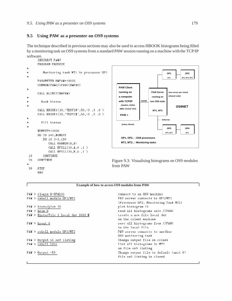
9.5. Using PAW as a presenter on OS9 systems 179
9.5 Using PAW as a presenter on OS9 systems
The technique described in previous sections may also be used to access HBOOK histograms being filledby a monitoring task on OS9 systems from a standard PAW session running on a machine with the TCP/IPsoftware.
INDIRECT PAWC
PROGRAM PRODUCE
Monitoring task MT� in processor OP��
PARAMETER NWPAW������
COMMON�PAWC�IPAWC�NWPAW�
CALL HLIMIT�NWPAW�
Book histos�
CALL HBOOK�����TEST�����������
CALL HBOOK�����TEST�����������
Fill histos�
NUMEVT������
DO �� I��NUMEVT
DO �� J�����
CALL RANNOR�AB�
CALL HFILL���A�����
CALL HFILL���B�����
�� CONTINUE
�� CONTINUE
�� STOP
END
PAW Client
running on
a computer
with TCP/IP
PAW >
(Apollos, SUNs)
(IBM, Central VAX)
(many clients)
PAW Server
running on
one OS9 node
MT1, MT2
OP1 OP2
OP3 OP4
MT1 MT1, MT2, MT3
MT1, MT2 MT1
TCP/IP
Ethernet
(one server per client)
(shared code)
OS9NET
OP1, OP2.. : OS9 processors
MT1, MT2.. : Monitoring tasks
Figure 9.3: Visualising histograms on OS9 modulesfrom PAW
Example of how to access OS9 modules from PAW
PAW � rlogin O�OPAL�� ! connect to an OS� machine
PAW � rshell module OP��MT� ! PAW server connects to OP��MT�
! �Processor OP� Monitoring Task MT��
PAW � histo�plot �� ! plot histogram ��
PAW � hrin � ! read all histograms into ��PAWC
PAW � Histo�File � local�dat ���� N ! create a new file local�dat
! on the client machine
PAW � hrout � ! save all histograms from ��PAWC
! to the local file
PAW � rshell module OP�MT� ! PAW server connects to another
! OS� monitoring task
PAW � Output �� os��listing ! Change output file on client
PAW � rshell ldir ! list all histograms in MT�
! on file os��listing
PAW � Output ��� ! Change output file to default �unit ��
! file os��listing is closed

Chapter 10: HBOOK Tabular Overview
Table 10.1: HBOOK Routine calling sequences
Calling Sequence page
CALL HARRAY �ID�NWORDS�LOC�� 56
CALL HBANDX �ID�YMI�YMA�VMX� 53
CALL HBANDY �ID�XMI�XMA�VMX� 53
CALL HBARX �ID� 54
CALL HBARY �ID� 54
CALL HBAR� �ID� 54
CALL HBFUN� �ID�CHTITL�NX�XMI�XMA�FUN� 55
CALL HBFUN� �ID�CHTITL�NX�XMI�XMA�NY�YMI�YMA�FUN� 55
CALL HBIGBI �ID�NCOL� 80
CALL HBINSZ ��YES���NO�� 52
CALL HBNAMC �ID�CHBLOK�IADDR�CHFORM� 25
CALL HBNAME �ID�CHBLOK�IADDR�CHFORM� 25
CALL HBNT �ID�CHTITL�CHOPT� 24
CALL HBOOKB �ID�CHTITL�NCX�XBINS�VMX� 51
CALL HBOOKN �ID�CHTITL�NVAR�CHRZPA�NPRIME�CHTAGS� 20
CALL HBOOKNC �ID�CHTITL�NVAR�BLOCK�TUPLE�CHTAGS� 27
CALL HBOOK� �ID�CHTITL�NX�XMI�XMA�VMX� 14
CALL HBOOK� �ID�CHTITL�NX�XMI�XMA�NY�YMI�YMA�VMX� 14
CALL HBPRO �ID�VMX� 52
CALL HBPROF �ID�CHTITL�NCX�XLOW�XUP�YMIN�YMAX�CHOPT� 51
CALL HBPROX �ID�VMX� 53
CALL HBPROY �ID�VMX� 53
CALL HBSET �OPTION�IVAL�IERR�� 24
CALL HBSLIX �ID�NSLI�VMX� 53
CALL HBSLIY �ID�NSLI�VMX� 53
CALL HCDIR ��CHPATH��CHOPT� 161
CALL HCOMPA �IDVECT�N� 81
CALL HCONVOL �ID��ID��ID�IERROR�� 38
CALL HCOPY �ID��ID��CHTITL� 17
CALL HCOPYM �ID�IPAWD�IOFSET� 173
variab hcreateg�global�name�base�common�size� 173
CALL HDDIR �CHPATH� 162
CALL HDELET �ID� 17
CALL HDERIV �DERIV� 116
CALL HDIFF �ID��ID��PROB��CHOPT� 101
180

181
Table 10.1: HBOOK Routine calling sequences (cont.)
Calling Sequence page
CALL HDIFFB �ID��ID��TOL�NBINS�CHOPT�NBAD��DIFFS�� 104
CALL HDUMP �ID� 98
CALL HERMES �LERR� 85
LOGVAR HEXIST �ID� 92
CALL HFC� �ID�IBIN�CLAB�W�CHOPT� 61
CALL HFC� �ID�IBINX�CLABX�IBINY�CLABY�W�CHOPT� 61
CALL HFF� �ID�NID�X�WEIGHT� 59
CALL HFF� �ID�NID�X�Y�W� 59
CALL HFILL �ID�X�Y�WEIGHT� 15
CALL HFINAM �ID�CHPNAM�NPAR� 114
CALL HFITEX �ID�AA��BB��CHI���IC�SIG�� 123
CALL HFITGA �ID�C��AV��SD��CHI���IC�SIG�� 123
CALL HFITH �ID�FUN�CHOPT�NP�PARAM��STEP�PMIN�PMAX�SIGPAR��CH��� 111
CALL HFITHN �ID�CHFUN�CHOPT�NP��PAR��STEP�PMIN�PMAX�SIGPAR��CHI��� 112
CALL HFITL �ID�FUN�NP��P��CHI���IC�SIG��COV��ST�PMI�PMA� 122
CALL HFITN �X�Y�EY�NPTS�N��NVAR�FUN�NP��P��CHI���IC�SIG��COV� 122
CALL HFITPO �ID�NP�A��CHI���IC�SIG�� 123
CALL HFITS �ID�FUN�NP��P��CHI���IC�SIG�� 122
CALL HFITV �N�NDIM�NVAR�X�Y�EY�FUN�CHOPT�NP�PARAM�STEP�PMIN�PMAX�SIGPAR�CHI�� 113
CALL HFIT� �X�Y�EY�N�FUN�NP��P��CHI���IC�SIG�� 123
CALL HFN �ID�X� 20
CALL HFNOV �ID�X� 21
CALL HFNT �ID� 27
CALL HFNTB �ID�CHBLOK� 27
CALL HFPAK� �ID�NID�V�N� 59
CALL HFUNC �ID�FUN� 55
variab hfree�global�size�base�common�offset� 174
CALL HF� �ID�X�WEIGHT� 58
CALL HF�E �ID�X�WEIGHT�ERRORS� 58
CALL HF� �ID�X�Y�WEIGHT� 59
CALL HGFIT �ID�NFPAR�NPFITS�FITCHI�FITPAR�FITSIG�FITNAM� 115
CALL HGIVE �ID�CHTITL��NX��XMI��XMA��NY��YMI��YMA��NWT��LOC�� 98
CALL HGIVEN �ID�CHTITL��NVAR��CHTAG��RLOW��RHIGH�� 31
CALL HGN �ID��IDN��IDNEVT�X��IERROR�� 31
CALL HGNF �ID�IDNEVT�X��IERROR�� 31
CALL HGNPAR �ID�CHROUT� 32
CALL HGNT �ID�IROW�IERR�� 33
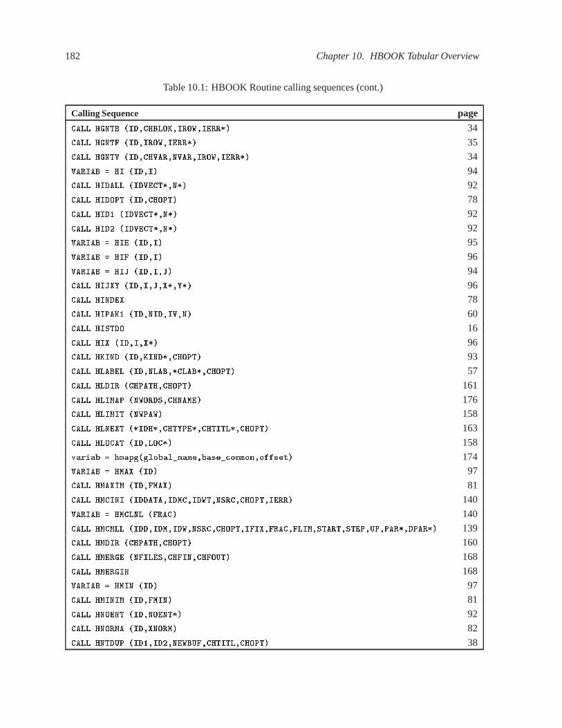
182 Chapter 10. HBOOK Tabular Overview
Table 10.1: HBOOK Routine calling sequences (cont.)
Calling Sequence page
CALL HGNTB �ID�CHBLOK�IROW�IERR�� 34
CALL HGNTF �ID�IROW�IERR�� 35
CALL HGNTV �ID�CHVAR�NVAR�IROW�IERR�� 34
VARIAB HI �ID�I� 94
CALL HIDALL �IDVECT��N�� 92
CALL HIDOPT �ID�CHOPT� 78
CALL HID� �IDVECT��N�� 92
CALL HID� �IDVECT��N�� 92
VARIAB HIE �ID�I� 95
VARIAB HIF �ID�I� 96
VARIAB HIJ �ID�I�J� 94
CALL HIJXY �ID�I�J�X��Y�� 96
CALL HINDEX 78
CALL HIPAK� �ID�NID�IV�N� 60
CALL HISTDO 16
CALL HIX �ID�I�X�� 96
CALL HKIND �ID�KIND��CHOPT� 93
CALL HLABEL �ID�NLAB��CLAB��CHOPT� 57
CALL HLDIR �CHPATH�CHOPT� 161
CALL HLIMAP �NWORDS�CHNAME� 176
CALL HLIMIT �NWPAW� 158
CALL HLNEXT ��IDH��CHTYPE��CHTITL��CHOPT� 163
CALL HLOCAT �ID�LOC�� 158
variab hmapg�global�name�base�common�offset� 174
VARIAB HMAX �ID� 97
CALL HMAXIM �ID�FMAX� 81
CALL HMCINI �IDDATA�IDMC�IDWT�NSRC�CHOPT�IERR� 140
VARIAB HMCLNL �FRAC� 140
CALL HMCMLL �IDD�IDM�IDW�NSRC�CHOPT�IFIX�FRAC�FLIM�START�STEP�UP�PAR��DPAR�� 139
CALL HMDIR �CHPATH�CHOPT� 160
CALL HMERGE �NFILES�CHFIN�CHFOUT� 168
CALL HMERGIN 168
VARIAB HMIN �ID� 97
CALL HMINIM �ID�FMIN� 81
CALL HNOENT �ID�NOENT�� 92
CALL HNORMA �ID�XNORM� 82
CALL HNTDUP �ID��ID��NEWBUF�CHTITL�CHOPT� 38
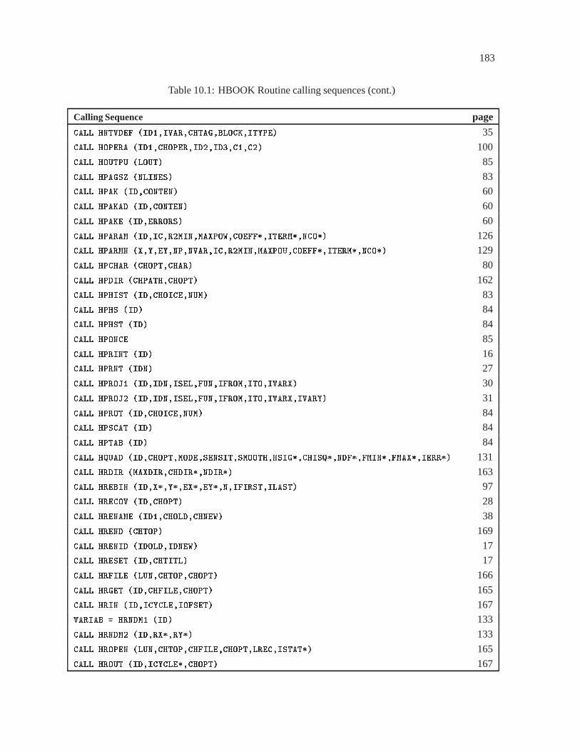
183
Table 10.1: HBOOK Routine calling sequences (cont.)
Calling Sequence page
CALL HNTVDEF �ID��IVAR�CHTAG�BLOCK�ITYPE� 35
CALL HOPERA �ID��CHOPER�ID��ID�C��C�� 100
CALL HOUTPU �LOUT� 85
CALL HPAGSZ �NLINES� 83
CALL HPAK �ID�CONTEN� 60
CALL HPAKAD �ID�CONTEN� 60
CALL HPAKE �ID�ERRORS� 60
CALL HPARAM �ID�IC�R�MIN�MAXPOW�COEFF��ITERM��NCO�� 126
CALL HPARMN �X�Y�EY�NP�NVAR�IC�R�MIN�MAXPOW�COEFF��ITERM��NCO�� 129
CALL HPCHAR �CHOPT�CHAR� 80
CALL HPDIR �CHPATH�CHOPT� 162
CALL HPHIST �ID�CHOICE�NUM� 83
CALL HPHS �ID� 84
CALL HPHST �ID� 84
CALL HPONCE 85
CALL HPRINT �ID� 16
CALL HPRNT �IDN� 27
CALL HPROJ� �ID�IDN�ISEL�FUN�IFROM�ITO�IVARX� 30
CALL HPROJ� �ID�IDN�ISEL�FUN�IFROM�ITO�IVARX�IVARY� 31
CALL HPROT �ID�CHOICE�NUM� 84
CALL HPSCAT �ID� 84
CALL HPTAB �ID� 84
CALL HQUAD �ID�CHOPT�MODE�SENSIT�SMOOTH�NSIG��CHISQ��NDF��FMIN��FMAX��IERR�� 131
CALL HRDIR �MAXDIR�CHDIR��NDIR�� 163
CALL HREBIN �ID�X��Y��EX��EY��N�IFIRST�ILAST� 97
CALL HRECOV �ID�CHOPT� 28
CALL HRENAME �ID��CHOLD�CHNEW� 38
CALL HREND �CHTOP� 169
CALL HRENID �IDOLD�IDNEW� 17
CALL HRESET �ID�CHTITL� 17
CALL HRFILE �LUN�CHTOP�CHOPT� 166
CALL HRGET �ID�CHFILE�CHOPT� 165
CALL HRIN �ID�ICYCLE�IOFSET� 167
VARIAB HRNDM� �ID� 133
CALL HRNDM� �ID�RX��RY�� 133
CALL HROPEN �LUN�CHTOP�CHFILE�CHOPT�LREC�ISTAT�� 165
CALL HROUT �ID�ICYCLE��CHOPT� 167

184 Chapter 10. HBOOK Tabular Overview
Table 10.1: HBOOK Routine calling sequences (cont.)
Calling Sequence page
CALL HRPUT �ID�CHFILE�CHOPT� 164
CALL HSCALE �ID�FACTOR� 82
CALL HSCR �ID�ICYCLE�CHOPT� 168
CALL HSETPR �CHNAME�VALUE� 128
CALL HSMOOF �ID�ICASE�CHI��� 130
VARIAB HSPFUN �ID�X�N�K� 131
CALL HSPLI� �ID�IC�N�K�CHI��� 130
CALL HSPLI� �ID�NX�NY�KX�KY� 131
CALL HSQUEZ ��YES���NO�� 83
CALL HSTAF �CHOPT� 80
VARIAB HSTATI �ID�ICASE�CHOICE�NUM� 99
VARIAB HSUM �ID� 98
CALL HTITLE �CHGTIT� 78
CALL HUNPAK �ID�CONTEN��CHOICE�NUM� 94
CALL HUNPKE �ID�CONTEN��CHOICE�NUM� 95
CALL HUWFUN �LUN�ID�CHFUN�CHFILE�ITRUNC�CHOPT� 35
VARIAB HX �ID�X� 94
VARIAB HXE �ID�X� 95
CALL HXI �ID�X�I�� 96
VARIAB HXY �ID�X�Y� 94
CALL HXYIJ �ID�X�Y�I��J�� 96

Bibliography
[1] L. Lamport. LATEX A Document Preparation System (Second Edition). Addison-Wesley, 1994.
[2] CN/ASD Group. HIGZ/HPLOT Users Guide, Program Library Q120 and Y251. CERN, 1993.
[3] CN/ASD Group. PAW users guide, Program Library Q121. CERN, October 1993.
[4] various authors. SUMX User’s Manual Program Library Y200. CERN, 1976. 1973 (Rev. 1976).
[5] R. Brun, M. Hansroul, and P. Palazzi. HBOOK users guide (Version 1.2), Program Library Y250.CERN, 1973.
[6] R. Brun, M. Hansroul, P. Palazzi, and B. Peuchot. HBOOK users guide (Version 2), Program LibraryY250 and DD/75/11. CERN, 1975.
[7] R. Brun, I. Ivanchencko, and P. Palazzi. HBOOK users guide (Version 3), Program Library Y250and DD/77/9. CERN, 1977.
[8] R. Brun, I. Ivanchencko, D. Lienart, and P. Palazzi. HBOOK users guide (Version 3 - Revised),Program Library Y250 and DD/EE/81-1. CERN, 1984.
[9] R. Brun and D. Lienart. HBOOK users guide (Version 4), Program Library Y250. CERN, 1987.
[10] CN/ASD Group and J. Zoll/ECP. ZEBRA Users Guide, Program Library Q100. CERN, 1993.
[11] W. T. Eadie, D. Drijard, F. James, M. Roos, and B. Sadoulet. Statistical Methods in ExperimentalPhysics. North-Holland, 1971.
[12] CN/ASD Group. MINUIT – Users Guide, Program Library D506. CERN, 1993.
[13] J. H. Friedman. Data Analysis Techniques for High Energy Particle Physics. In CERN, editor,Proceedings of the 1974 CERN School of Computing, Godoysund (Norway), 1974. CERN Report74-23.
[14] B. Schorr. Spline estimation of Distributions and Density Functions. Technical Report DD/75/13,CERN, 1975.
[15] B. Schorr. Etude du lissage d’histogramme par la methode des B-splines et implementation dansHBOOK. Technical Report DD/EE/78-3, CERN, 1978.
[16] J. Allison. Multiquadratic Radial Basis Functions for Representing Multidimensional High EnergyPhysics Data. Comp. Phys. Comm., 77:377–395, 1993.
[17] Roger Barlow and Christine Beeston. Fitting using finite Monte Carlo Samples. Comp. Phys.Comm., 77:219, 1993.
[18] Roger Barlow. Fitting using finite Monte Carlo Samples. J. Comp. Phys., 72:202, 1987.
[19] CERN. CSPACK – Client Server Computing Package, Program Library Q124, 1991.
185

Index
�N�, 114�Q�, 166�S�, 61�SA�, 57�U�, 61, 115/PAWMAP/ common, 1733530h, 129
access to histogram information, 92add histograms, 100analytic function, 123array, 60attribute, 158
B-splines, 129band, 158bin
histogram rebinning, 97BLAC, 80block, 26BSIZE, 25
CERNVM, 170change directory, 171channel contents, 92character type, 4CHFILE, 165, 166Chisquare test, 102CHOPT, 24circular buffer, 21CLABX, 61CLABY, 61client, 179common /PAWMAP/, 173common �PAWC�, 4, 5, 18, 19, 25, 56, 98, 129,
157, 158, 160, 173, 176confidence level, 103Convolution
Ntuple, 38covariance matrix, 124current directory, 22, 171CWN, see Ntuple, Column-Wise-Ntuple
data acquisition system, 173data structure, 157data summary tape, 18
DecStation, 176Deprecated routines, 122–123difference
between histograms, 101direct access file, 164directory, 160, 171
change, 171current, 22, 171
divide histograms, 100DST, 1, 8, see data summary tapeDuplicate
Ntuples, 38
EDM, 120, 122elementary function, 123equivalent event, 99ERRO, 54error, 60, 158
return codes, see IQUESTerrors on fitted parameters, 117exchange mode, 170existence of histogram, 92expansion of function, 123exponential
fit, 112
F-test, 124fit, 110
exponential, 112gaussian, 112polynomial, 112
fitting, 110–116fitting Monte Carlo statistics, 133–156floating number, 59Fortran, 92Fortran convention, 4FPARAM, 129ftp, 170FUN, 115, 116
gaussianfit, 112
global section, 173, 175, 177global�sect, 175–177
H�EVLI, 93
186

INDEX 187
H�PAGE, 93HARRAY, 16, 56HBANDX, 53, 53HBANDY, 53HBAR�, 54, 54HBARX, 54, 54, 56, 58, 60, 93, 95, 100, 102, 110,
126, 160HBARY, 54, 54, 59, 93HBASFT, 127HBFUN�, 55, 80, 133HBFUN�, 55, 133HBIGBI, 80, 80, 93HBINSZ, 52, 52HBLACK, 93HBNAMC, 18, 24, 25, 26, 27, 33–35HBNAME, 18, 24, 25, 26, 27, 33–35HBNT, 18, 24, 24, 25, 27, 29, 35, 160HBOOK, 1, 12, 56, 116, 157, 158, 160, 161, 164,
165, 170, 171HBOOK�, 5, 14, 30, 51, 53, 55, 78, 80, 93, 160HBOOK�, 5, 14, 55, 57, 80, 93HBOOKB, 51HBOOKN, 18, 20, 21, 22, 27, 31, 32, 160HBOOKNC, 27HBPRO, 52, 53HBPROF, 51HBPROX, 53HBPROY, 53HBSET, 19, 23, 24HBSLIX, 53, 53HBSLIY, 53HBSTAT, 93HCDIR, 24, 161, 167, 171, 173�HCFITD� fit parameters common, 111, 113, 115HCOMPA, 81HCONVOL, 38HCOPY, 17HCOPYM, 173hcreateg, 173HDDIR, 162HDELET, 17HDERIV, 111–113, 116, 117HDIFF, i, 101, 101, 102–106, 168HDIFFB, i, 104, 105, 106, 108, 109HDUMP, 98HELEFT, 127
HERMES, 85, 85HERROR, 93HESSE, 111, 112, 114, 118, 140HEXIST, 92, 92HF�, 58, 58, 59HF�E, 58HF�, 54, 58, 59, 59HFC�, 57, 61, 61, 62HFC�, 57, 61, 61, 62HFCNH, 116HFCNV, 116HFF�, 59, 59HFF�, 59HFILL, 5, 15, 51, 54, 58, 59HFINAM, 114, 115HFIT�, 123HFITEX, 123HFITGA, 123HFITH, 110, 111, 114–116, 119, 122HFITHN, 110, 112, 114, 115, 123HFITL, 122HFITN, 116, 122HFITPO, 123HFITS, 122HFITV, 110, 113, 115, 116, 119, 122, 123HFN, 18, 20, 21, 22HFNOV, 21, 21HFNT, 18, 24, 27, 27, 29, 46HFNTB, 18, 23, 27HFPAK�, 59, 60hfree, 174HFUNC, 55, 56, 80, 93, 160HGFIT, 115HGIVE, 98HGIVEN, 31HGN, 18, 31, 31, 32HGNF, 18, 31, 32, 32HGNPAR, 31, 32, 32HGNT, 18, 25, 33, 35HGNTB, 18, 25, 34, 35, 37HGNTF, 18, 25, 35HGNTV, 18, 25, 34, 34, 35, 37HI, 94, 94HID�, 92, 92HID�, 92HIDALL, 92
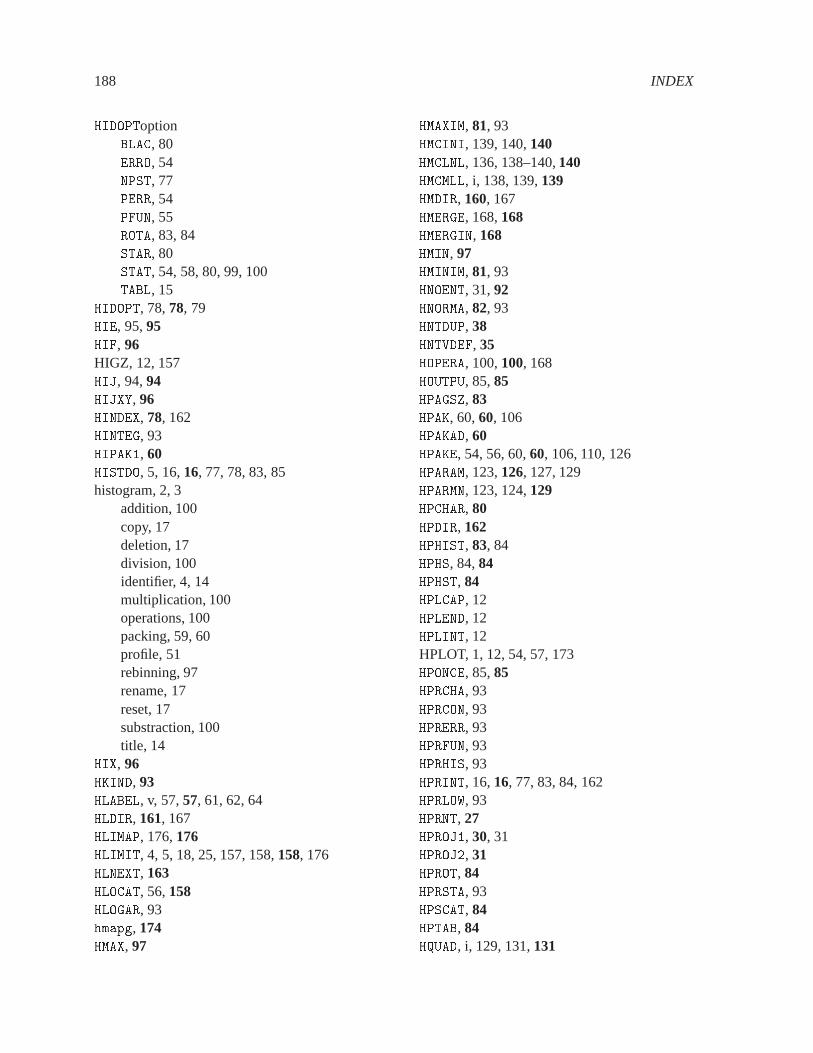
188 INDEX
HIDOPToptionBLAC, 80ERRO, 54NPST, 77PERR, 54PFUN, 55ROTA, 83, 84STAR, 80STAT, 54, 58, 80, 99, 100TABL, 15
HIDOPT, 78, 78, 79HIE, 95, 95HIF, 96HIGZ, 12, 157HIJ, 94, 94HIJXY, 96HINDEX, 78, 162HINTEG, 93HIPAK�, 60HISTDO, 5, 16, 16, 77, 78, 83, 85histogram, 2, 3
addition, 100copy, 17deletion, 17division, 100identifier, 4, 14multiplication, 100operations, 100packing, 59, 60profile, 51rebinning, 97rename, 17reset, 17substraction, 100title, 14
HIX, 96HKIND, 93HLABEL, v, 57, 57, 61, 62, 64HLDIR, 161, 167HLIMAP, 176, 176HLIMIT, 4, 5, 18, 25, 157, 158, 158, 176HLNEXT, 163HLOCAT, 56, 158HLOGAR, 93hmapg, 174HMAX, 97
HMAXIM, 81, 93HMCINI, 139, 140, 140HMCLNL, 136, 138–140, 140HMCMLL, i, 138, 139, 139HMDIR, 160, 167HMERGE, 168, 168HMERGIN, 168HMIN, 97HMINIM, 81, 93HNOENT, 31, 92HNORMA, 82, 93HNTDUP, 38HNTVDEF, 35HOPERA, 100, 100, 168HOUTPU, 85, 85HPAGSZ, 83HPAK, 60, 60, 106HPAKAD, 60HPAKE, 54, 56, 60, 60, 106, 110, 126HPARAM, 123, 126, 127, 129HPARMN, 123, 124, 129HPCHAR, 80HPDIR, 162HPHIST, 83, 84HPHS, 84, 84HPHST, 84HPLCAP, 12HPLEND, 12HPLINT, 12HPLOT, 1, 12, 54, 57, 173HPONCE, 85, 85HPRCHA, 93HPRCON, 93HPRERR, 93HPRFUN, 93HPRHIS, 93HPRINT, 16, 16, 77, 83, 84, 162HPRLOW, 93HPRNT, 27HPROJ�, 30, 31HPROJ�, 31HPROT, 84HPRSTA, 93HPSCAT, 84HPTAB, 84HQUAD, i, 129, 131, 131

INDEX 189
HRDIR, 163HREBIN, 97HRECOV, 28HRENAME, 38HREND, 27, 29, 165, 166, 169, 169, 171HRENID, 17HRESET, 17HRFILE, 20, 161, 166, 166, 167, 169, 171, 173HRGET, 165, 165HRIN, 157, 161, 165, 167, 168, 173HRNDM�, 133, 133HRNDM�, 133HROPEN, 18–25, 27, 160, 165, 165, 166, 167, 170,
171HROTAT, 93HROUT, 24, 27–29, 114, 157, 161, 165, 167, 167,
173HRPUT, 164, 165HRVAL, 125HSCALE, 82, 93HSCR, 168HSELBF, 125, 127, 128HSETPR, 125, 127, 128, 128HSMOOF, 129, 130HSPFUN, 129, 131HSPLI�, 129, 130, 130, 131HSPLI�, 129, 131HSQUEZ, 83HSTAF, 80HSTAR, 93HSTATI, 99, 109HSUM, 98HTABLE, 77, 93HTITLE, 5, 78HUNPAK, 83, 94, 99HUNPKE, 95HUWFUN, 25, 33, 35, 35, 36HX, 94HXE, 95HXI, 96HXY, 94HXYIJ, 96
I/O, 164IBINX, 61, 62IBINX��, 61
IBINY, 61IBINY��, 61identifier, 4input, 164integer number, 60integer type, 4IQUEST communicationvector, 22, 111, 112, 164,
166
Kolmogorov test, 101, 102KUIP, 157
limits on fitted parameters, 117line printer, 16log-likelihood, 110LREC, 170LRECL, 18, 19
mean value, 92, 99memory, 21MIGRAD, 117, 118minimisation, 110MINOS, 111, 112, 114, 140MINUIT, 112, 113, 116–122, 139mononomial, 123Monte Carlo statistics, 133–156multiply histograms, 100multiquadric, 129MZEBRA, 4
NFPAR, 115nfs, 170NPST, 77NTUPLE, 93Ntuple, 2, 3, 18–50, 164, 165
Column-Wise-Ntuple, 18, 19, 22–28, 33, 35,37, 46, 168
convolution, 38disk resident, 20, 21duplicate, 38identifier, 4memory resident, 20, 21operation, 38rename column, 38reset, 17Row-Wise-Ntuple, 18, 20, 21, 23, 27, 31, 32,
35, 38, 40, 168

190 INDEX
null hypothesis, 103NWBUFF, 18, 21NWPAWC, 158
one-dimensional histogram, 14online, 164OS9, 179output, 164overflow, 99
packing, 4, 14, 59, 60parameter
errors (fit), 117parameter type, 4parametrization, 123–129pathname, 171PAW, 1, 18, 21–23, 27, 31, 35, 37, 45, 54, 57, 80,
111, 116, 117, 119, 131, 157, 168, 171,173, 176, 178
server, 179PAW++, 170�PAWC� common, 4, 5, 18, 19, 25, 56, 98, 129,
157, 158, 160, 173, 176PAWMAP common, 173PERR, 54PFUN, 55Poisson distribution, 110polynomial
fit, 112presenter, 175, 177, 179print, 16profile histogram, 51projection, 60, 158
�QUEST�, see IQUEST
random number generation, 133real type, 4rebinning, 97regressor, 124remote
file, 178login, 178, 179shell, 178, 179
Renamecolumn in Ntuple, 38
Reset
histogram, 17Ntuple, 17
resize command (VMS), 170RLOGIN, 178, 179ROTA, 83, 84RSHELL, 178, 179RWN, see Ntuple, Row-Wise-NtupleRZ file, 18RZ package of ZEBRA, 164RZPURG, 167
saturation, 102scatter-plot, 2server, 179shared memory, 176, 177slice, 60Smirnov-Cramer-Von-Mises test, 103smoothing, 129–132standard deviation, 92, 99STAR, 80STAT, 54, 58, 80, 99, 100subscract histograms, 100Sun, 176
TABL, 15table, 2Taylor expansion, 123TCP/IP, 179test
Kolmogorov, 101TKOLMO, 103two-dimensional histogram, 14type
character type, 4integer, 4parameter, 4real, 4
underflow, 99Unix, 160, 165, 166, 170, 176, 177
VAX, see VMSVAX/VMS, 175VM/CMS, 165, 166, 171VMS, 170, 171, 175VMX, 4, 14VMX, 160

INDEX 191
W, 61weight, 15
XZRZOP, 162
ZEBRA, 157–160, 164, 167, 171RZ package, 164, 171