CEO Turnover in a Competitive

Assignment Framework

Andrea L. Eisfeldt∗ Camelia M. Kuhnen†

February 2010

Abstract

This paper considers the empirical stylized facts about CEO turnover in thecontext of a competitive assignment model in which CEOs and firms form matchesbased on multiple characteristics. CEOs are viewed as hedonic goods with multidi-mensional skill bundles. Likewise, firms’ production functions have heterogeneousweights on CEO skills such as firm-specific knowledge, ability to grow sales, andability to cut costs. There exists a competitive market for CEOs, whose wages aredetermined analogously to the prices of the hedonic goods in Rosen (1974). Thecompetitive assignment framework with multiple skill dimensions is able to captureseveral stylized facts which are not explained by existing theories. For example,in our model, both poor relative performance and poor absolute performance areassociated with higher rates of CEO turnover. Relative performance evaluationmatters even though there is no agency problem or learning, and overall industryperformance affects turnover as well. Our model also makes predictions about thetype and pay of the replacement manager conditional on turnover type which areconsistent with patterns we document empirically. For example, managers who arefired are more likely to be replaced by industry outsiders than are managers whoquit or retire. Moreover, replacement managers in these cases earn significantlymore than the incumbent. To document pay and replacement type as a functionof the type of turnover event, we construct a large dataset describing turnoverevents during the period 1992-2006, including the type of turnover event, and thecharacteristics and pay of the replacement manager.

∗Department of Finance, Kellogg School of Management, Northwestern University, 2001 SheridanRd., Evanston, IL 60208-2001, a-eisfeldt@northwestern.edu

†Department of Finance, Kellogg School of Management, Northwestern University, 2001 SheridanRd., Evanston, IL 60208-2001, c-kuhnen@kellogg.northwestern.edu.

1 Introduction

This paper considers the empirical stylized facts about CEO turnover in the context

of a competitive assignment model in which CEOs and firms form matches based on

multiple characteristics. CEOs are viewed as hedonic goods with multidimensional skill

bundles. Likewise, firms’ production functions have heterogeneous weights on CEO skills

such as firm-specific knowledge, ability to grow sales, and ability to cut costs. There

exists a competitive market for CEOs, whose wages are determined analogously to the

prices of the hedonic goods in Rosen (1974). The competitive assignment framework with

multiple skill dimensions is able to capture several stylized facts which are not explained

by existing theories. For example, in our model, both poor relative performance and

poor absolute performance are associated with higher rates of CEO turnover. Relative

performance evaluation matters even though there is no agency problem or learning, and

overall industry performance affects turnover as well. Our model also makes predictions

about the type and pay of the replacement manager conditional on turnover type which

are consistent with patterns we document empirically. For example, managers who are

fired are more likely to be replaced by industry outsiders than are managers who quit

or retire. Moreover, replacement managers in these cases earn significantly more than

the incumbent. To document pay and replacement type as a function of the type of

turnover event, we construct a large dataset describing turnover events during the period

1992-2006, including the type of turnover event, and the characteristics and pay of the

replacement manager.

There is considerable controversy about both CEO pay and CEO retention. Recently,

papers such as Tervio (2008) and Gabaix and Landier (2008) have shown that viewed

through the lens of competitive assignment models based on that in Rosen (1981), the

observed high levels of CEO pay can be seen as natural outcomes of the joint distribution

of talent and firm sizes.1 These papers constitute one response to the argument that the

observed high level of CEO pay is a result of entrenched managers earning excessive rents

(eg. Bebchuk and Fried (2004)).

In this paper, we ask whether the implications of a competitive assignment model

can also be used to understand the flip side of CEO pay, namely CEO turnover. As with

1See also the early contribution by Lucas (1978), the competitive assignment model of the distributionof earnings in Sattinger (1979) and the review of the implications of competitive assignment models forearnings in Sattinger (1993). Dicks (2009) studies the implications of the assignment model of CEO payfor corporate governance.

1

CEO pay, there is a debate over whether boards optimally decide to terminate or retain

their manager. Several papers have asked whether considering the board’s monitoring

problem in the moral hazard and asymmetric information setting of Holmstrom (1982)

and Gibbons and Murphy (1990) can explain observed patterns in turnover events and

have shown that indeed poor performing managers are less likely to be retained.2 How-

ever, others (Jenter and Kanaan (2006) and Kaplan and Minton (2006)) have recently

noted that industry conditions also contribute significantly to the termination decision,

with poor industry conditions leading to a higher likelihood of turnover. In this paper,

we illustrate how a competitive assignment model like those used to explain the distri-

bution of CEO pay can be used to understand these observed empirical patterns of CEO

turnover.

That decisions about CEO replacement can be driven by industry conditions and

observable managerial characteristics can be seen clearly in current events. The future of

the CEOs in the beleaguered US auto and financial services industries is being debated

by the media and influenced by government interventions. However, not all CEOs face

the same termination risk. For example, the US government forced GM’s Rick Wagoner

out by threatening to withhold further bailout money, but allowed Chrysler’s Robert

Nardelli to stay on. In an article about the replacement, the Wall Street Journal3 noted

that, “Unlike Mr. Wagoner, who had been at the helm of GM since 2000, Mr. Nardelli is

considered an auto-industry outsider”. Similarly, there has been speculation that CEOs

in the financial services industry, such as Vikram Pandit of Citigroup and Ken Lewis of

Bank of America might also be ousted.4 However, given the complexity of the assets of

certain financial institutions, firm-specific and industry specific knowledge may be critical

to weathering financial crises and this may make outsider replacements untenable.

Our theoretical framework is based on a competitive assignment environment, where

both the CEO and the firm optimize over the relative value of preserving their current

match vs. pursuing their outside option. We model managers as hedonic goods with mul-

tiple characteristics, or skills. Likewise, firms have production functions whose weights

on these skills may vary both in the cross section and over time. We show that shocks

to the weights on skills such as firm-specific knowledge, ability to grow sales, and ability

2See for example Barro and Barro (1990), Gibbons and Murphy (1990), and Warner, Watts, andWruck (1988).

3March 30 2009 issue, available on-line at http://online.wsj.com/article/SB123836090755767077.html.4In fact, in September 2009 Ken Lewis announced that he will step down as the CEO of Bank of

America.

2

to cut costs, can generate turnover that is correlated with both poor relative and ab-

solute performance. We argue that the competitive assignment model can also be used

to understand the choice between an inside and outside replacement manager, and the

corresponding pay and performance of the replacement. Viewing managers as hedonic

goods allows one to consider how industry shocks might drive CEO turnover since weights

on particular skills are likely to be correlated within industries. In future work, it may

also be interesting to use a hedonic pricing model to understand which of the scarce

skills general managers possess drives the high pay of talented CEO’s. For example,

Murphy and Zabojnik (2004), Murphy and Zabojnik (2007) and Frydman (2005) have

used the hypothesis that general managerial skills have increased in importance relative

to firm-specific skills to understand the rise in CEO pay over time. However, in this

paper we focus mainly on turnover events, and study the dynamics of CEO pay only

around turnover events.

Our empirical work contributes to the existing literature by studying a large dataset

of CEO replacements we construct to describe turnover events which occur during the

period 1992-2006. We collect information regarding both the reason for the incumbent

CEO’s departure and the identity and background of the new CEO. We study the effect of

firm and industry conditions on the likelihood of turnovers classified as forced departures,

potential quits or retirements. We similarly document the determinants of the choice of

whether the replacement CEO will be a firm insider, industry insider, or firm and industry

outsider. Empirically, a large fraction of turnover events cannot be classified as either

firings or quits. Interestingly, in the context of a competitive assignment model where

separations occur when total surplus becomes negative, this is also the case. Under most

reasonable theoretical definitions of fires vs. quits, a large fraction of separations in data

generated by the model would remain unclassified.

First, we show that our dataset confirms earlier findings that poor industry stock

returns and low firm stock performance relative to the industry increase the likelihood of

forced turnover. Controlling for firm relative to industry stock returns, we find that low

firm relative to industry return on assets (ROA) also increases the likelihood of forced

turnovers. Thus, real variables contain additional information about CEO performance.

Not surprisingly, retirements and potential quits appear to be much less affected by rela-

tive firm performance than are forced turnovers. Poor firm performance still significantly

increases the likelihood of these types of turnovers too, but the magnitude of the effect is

less than a quarter of the effect of poor performance on the likelihood of forced turnovers.

3

Our empirical work supports the idea that the independent effects of industry condi-

tions on turnover may be driven by the fact that industry shocks can change what type

of manager is optimal. For example, industries which experience a decline in the long

term trend of return on assets, have lower stock returns, or have lower average ROA

also experience more forced turnovers. Importantly, firms that force departures are more

likely to choose a replacement CEO from outside the industry, consistent with the idea

that the firm desires to match with a new manager with a different skill set than that of

the incumbent.

We also show that industry conditions affect the CEO’s decision to depart the firm

voluntarily. Potential quits are more frequent in industries with down-trending ROA,

and with lower average stock returns and ROA, suggesting that in those industries the

outside option of the CEO of leisure or perhaps joining private firms is more valuable than

the expected payments received by staying with the firm during the industry downturn.

Retirements are less frequent in industries with higher employment growth, possibly

indicating that part of the rent captured by active CEOs comes from empire building

(e.g. managing organizations with many employees).

Replacement CEOs are significantly more likely to come from outside the firm and

outside the industry when the firm does poorly in terms of stock returns and return

on assets, or when the industry has low ROA, which are instances where typically the

incumbent CEO is fired. Replacement CEOs are more likely to come from inside the firm

if the turnover event was due to retirement or voluntary departure rather than forced

turnover. The pay of replacement CEOs is highest in situations where the incumbent

was fired and the new CEO is an outsider.

Our paper builds on the results of a large body of work5 on CEO turnover. One of the

most documented facts is that relative performance evaluation (RPE) matters for CEO

turnover: the probability of CEO turnover is negatively related to the performance of

the firm relative to the industry (Barro and Barro (1990), Gibbons and Murphy (1990))

or to the market (Warner, Watts, and Wruck (1988)).

However, RPE does not seem to be the only driver of managerial changes. Jenter and

Kanaan (2006) document that CEOs are more likely to be dismissed from their job after

bad industry and bad market performance, and in light of these findings argue that RPE

cannot be the sole determinant of CEO turnover. They suggest two hypotheses consistent

with the empirical results. First, corporate boards may commit systematic attribution

5See Murphy (1999) for a review of the literature on CEO compensation and turnover.

4

errors and credit or blame the CEO for performance caused by factors outside their

control. Second, firm performance in bad times may be more revealing about CEO skill

than performance in good times. In our model, the relevance of industry conditions for

whether or not a CEO is forced out comes from considering the firm and CEO as parties

in a match whose actions depend on their respective outside options. The data seem to

support this idea since the type of turnover event helps to predict the type of replacement

chosen. In particular, forced turnovers are associated with replacement by outsiders.

Several papers have focused on the relationship between corporate governance, com-

pensation and CEO turnover. Huson, Parrino, and Starks (2001) find that the frequency

of forced turnover and of outside succession increased over time during 1971 to 1994, and

that board characteristics influence the likelihood of these events. Kaplan and Minton

(2006) argue that the CEO turnover rate during 1992-2005 is higher than previously

found for the prior two decades (11.8% versus 10%) and attribute this to boards becom-

ing increasingly more sensitive to the CEO’s performance.6 Peters and Wagner (2007)

suggest that this recent increase in turnover has lead to a significant increase in CEO

pay, as executives face a higher risk of losing their jobs.

The role of industry conditions on CEO turnover has not received much attention

in the literature. This may be because historically, the literature on CEO turnover

has focused on the role of boards as monitors of the firm and has attempted to ascer-

tain their effectiveness in this role.7 Notable exceptions are Parrino (1997) and Eisfeldt

and Rampini (2008). Parrino (1997) argues that intra-industry CEO appointments are

less costly and performance measures are more precise in homogeneous industries, and,

consistent with this argument, finds that the likelihood of forced turnover and of an intra-

industry appointment increase with industry homogeneity. Eisfeldt and Rampini (2008)

show how aggregate business cycle conditions can drive CEO turnover and compensation

in a principal agent environment where managers have private information about their

skill. Their focus, however, is on external turnover due to mergers and acquisitions.

6Kaplan and Minton (2006) also document that CEO turnover is related to industry performancerelative to the stock market, and performance of the overall stock market, but do not provide an inter-pretation for these results, as they are not the focus of the paper.

7We thank Robert Parrino for this helpful historical perspective on the literature.

5

2 Model

Our model is similar to the competitive assignment models used to explain the rise in, and

high levels of CEO compensation, except that in those models skill is one-dimensional

and there is only one industry. In fact, we believe we are the first to develop a com-

petitive assignment model with two industries, or markets, although the two market set

up might be useful for modeling marriage markets, general labor markets, or real estate

markets as well. Having two industries is useful for studying turnover, but it does add

complication since firm and manager outside options depend on conditions in both in-

dustries. Similarly, one dimensional heterogeneity across managers and firms is a useful

simplification which allows one to derive managers’ wage profiles as a function of talent

in a straightforward manner.

Our modeling strategy is most closely related to Tervio (2008) who uses the model

from Sattinger (1979) in which skills are one-dimensional, skill and size distributions are

continuous, and firm size and CEO ability are complementary in production, to analyti-

cally describe the relationship between CEO talent, firm size, and CEO pay. Gabaix and

Landier (2008) employ extreme value theory to show quantitatively that such a model can

explain the rise in and level of CEO pay. Finally, in a closely related model, Murphy and

Zabojnik (2004) and Murphy and Zabojnik (2007) incorporate firm-specific vs. general

skill by modeling firms as only being able to deploy a fraction of a new CEO’s ability. The

remaining fraction represents firm-specific skill which can only be deployed by incumbent

managers. Murphy and Zabojnik use their model to explain the rise in CEO pay by an

increase in the importance of general managerial skills through comparative statics over

this fraction. Our model and solution methods will closely follow Tervio (2008) adapted

to our set up with multidimensional heterogeneity and more than one industry.

There are two dates, zero and one. At each date, managers will be matched to

firms via competitive assignment. To fix ideas, it is useful to first examine the decision

problems of a single firm and manager at a single date. For this, we consider the decision

problems of a manager and a firm who are currently matched in a competitive assignment

economy. Neither the firm, nor the manager can commit to honoring long term contracts,

so each must earn at least the value of their outside option in each period in order for the

match to continue. The dynamics of optimal managerial compensation induced by agency

problems when long term contracts are feasible is the focus of many recent theoretical

6

papers.8 Although some of these papers do contain results about contract termination,

their main focus is on compensation dynamics rather than CEO turnover. For the most

part termination in these models is rare, and is largely used as a stick to provide incentives

with rather than treated as an object of interest in and of itself. The limited focus on

CEO turnover in the theoretical literature is in contrast to the large empirical literature

on turnover discussed above.

We consider a firm i which produces output using capital and the managerial input

from manager j according to:

ai(mj)kα,

where ai(mj) is the productivity of capital when firm i employs manager j, and α ∈ [0, 1].

This productivity is given by (slightly abusing notation):

ai(mj) =S∑

s=1

θi,saj,s

where θi,s is a weight which describes the importance of skill s in determining the pro-

ductivity of capital deployed in firm i and aj,s is the level of ability of manager j in skill s.

Thus the productivity of manager j employed at firm i is the inner product of manager

j’s skill levels and firm i’s skill weights. These weights vary over time and across firms.

Moreover, these weights are likely to be correlated within industries, and subject to com-

mon shocks. For example, growing firms may have high weights on skills such as building

and motivating a sales force, and firms in mature industries may place higher weights on

cost cutting. Firms which can fund growth or operating leverage internally may not have

a high weight on the ability to raise external finance, whereas firms needing to access

capital markets might. Similarly, the importance of firm-specific vs. general skills may

vary in the spirit of the evidence documented by Frydman (2005) for the time series of

all firms. The abilities of managers may also vary over time. In particular, managers

8See for example, DeMarzo and Fishman (2007a), DeMarzo and Fishman (2007b), He (2007),DeMarzo, Fishman, He, and Wang (2009), He (2009), Sannikov (2008), and Lustig, Syverson, andVan Nieuwerburgh (2009). Sannikov (2008) considers the effects of variation in firm and managerialoutside options on the agency costs of providing incentives. DeMarzo, Fishman, He, and Wang (2009)consider how exogenous variables affect the degree of agency costs and hence the dynamics of managerialcompensation. Lustig, Syverson, and Van Nieuwerburgh (2009) study how managerial outside optionsaffect the division of rents between managers and firm owners over time and study the induced distribu-tions of managerial compensation. He (2007) focuses on the effects of hidden savings on compensationdynamics. Edmans and Gabaix (2009) provide a survey of how these and other recent theories canexplain “pay-for-luck”.

7

may gain firm-specific abilities through learning by doing during their tenure with the

firm. Although it is interesting to consider the decision by the manager to invest in ac-

cumulating different skills, for simplicity here we will assume that abilities are fixed and

leave a study of that investment decision for future work.9 Bertrand and Schoar (2003)

document managerial fixed effects in management style, consistent with abilities being

somewhat rigid. For it to be optimal to replace a manager with a suboptimal skill set,

we need to have that there are at least investment costs, adjustment costs, or time to

build for managerial skills, which seems reasonable. The value or total surplus created

by firm i when it is matched with manager j is

V ≡ ai(mj)kα.

To keep things simple, there is no labor other than the managerial input in our model.

Since we assume that there is no commitment on the part of the manager, the manager

will always need to earn a value inside the match equal to the value of their outside

option. The manager can quit, or they can retire. We assume that there is a market

for managers in which the per period hedonic price of a manager is given by the market

value of that manager’s ability bundle, which we denote by wj. This market is in the

spirit of that formalized in Rosen (1974) and Lancaster (1966). Rosen (1974) contains a

description of the technical assumptions which determine the properties of the hedonic

price function. If skill bundles are recombinable, and there is no arbitrage, this function

will be linear but these assumptions seem strong for the CEO market and so we expect

the price function to be nonlinear. Moreover, because bundles cannot be dismantled, the

price of any particular skill will depend on the joint distributions of and demands for

all skills. For this reason, when one is interested in the distribution of CEO pay it is

convenient to assume that skills are one-dimensional, as in Sattinger (1979) and Tervio

(2008). Here, we depart from this assumption but simplify our general model in order to

solve for managerial wages. We illustrate ideas by solving a simple example in Subsection

2.1. Then, in Subsection 2.2 we solve a two industry version of our model with skill levels

and weights carefully specified to allow us to solve the model for turnover and wages in

a parsimonious way. We base our solution method on that in Tervio (2008)) adapted to

incorporate the additional heterogeneity and the existence of an alternative industry for

9In a recent paper Giannetti (2009) presents a model where compensation is designed to incentivizemanagers to invest in firm-specific skills.

8

managers.

If the manager can either stay at his current employer, quit for his next best employ-

ment option, or retire, then the manager’s outside option is:

V mj ≡ max {wj, R}

where R is the value of retiring.

The firm’s owners will also need to be paid their outside option. The firm can fire the

manager and hire a replacement, or it can liquidate. The firm’s outside option is given

by:

V fi ≡ max{

maxn{ai(mn)kα − (V mn)} , L

}.

The left hand argument is the value the firm receives with the optimal replacement

manager, where ai(mn) and V mn are defined analogously to the productivity of manager

j at firm i and the outside option of manager j defined above as a function of the market

prices of manager n’s skills. The right hand argument, L, is the liquidation value of the

firm.

The current match will dissolve if total surplus from the match is negative, in other

words if the value created by the current match after payments to capital and labor,

minus the manager’s outside option, minus the firm’s outside option, is negative, i.e. if:

(ai(mj)kα)− (max {wj, R})

− (max {maxn {ai(mn)kα − (V mn)} , L}) < 0

or,

V − V mj − V fi < 0.

This condition is analogous to what Murphy and Zabojnik (2004) describe as the “make

or buy” tradeoff, except that skills are multidimensional.

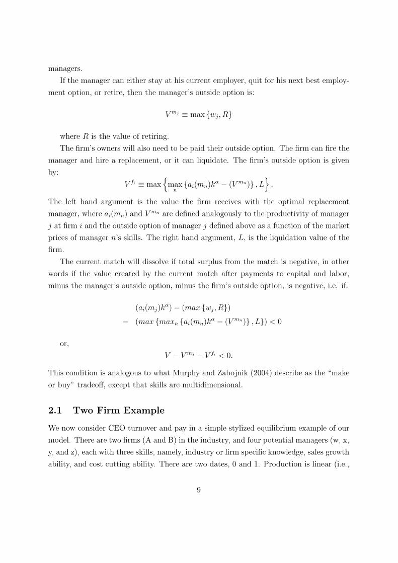
2.1 Two Firm Example

We now consider CEO turnover and pay in a simple stylized equilibrium example of our

model. There are two firms (A and B) in the industry, and four potential managers (w, x,

y, and z), each with three skills, namely, industry or firm specific knowledge, sales growth

ability, and cost cutting ability. There are two dates, 0 and 1. Production is linear (i.e.,

9

α = 1), the interest rate is zero, there is no labor, and capital k is fixed. At date 0, Firm

A has 3 units of capital and θ weights (1, 1, 0) on the 3 skills respectively. Firm B has 1

unit of capital and θ weights (0, 1, 0) on the 3 skills respectively. Thus, both firms weight

sales growth ability, and firm A weighs industry specific skills more heavily (it produces

a more complex good, for example). Manager w has skill levels (1, 1, 0), manager x has

skill levels (0, 1, 0), manager y has skill levels (0, 0, 1), and manager z has skill levels (0,

0, 3), for the 3 skills respectively. Thus, manager w has industry specific skills and sales

growth skills, manager x has sales growth skills, and managers y and z have cost cutting

skills. Managers who do not get hired may deploy their non-industry specific skills in

another industry which has weights equal to one on sales growth and cost cutting and

capital equal to 12. Firms in this alternative industry face free entry and earn zero profits,

thus, managers’ who are not hired have outside options equal to 12

∑s=2:3 as.

An equilibrium at date 0 is an allocation of managers to firms, and wages paid to

managers, such that no manager and no firm prefers an alternative allocation.10 One

such equilibrium is as follows: Firm B hires manager x, produces 1 unit of output, pays

the manager 12

+ ε in order to make the manager prefer to work at firm B instead of in

the alternative industry, and has profits of 12− ε. Firm A hires manager w, produces 6

units of output, pays the manager 12

+ 2ε in order to make the manager prefer to work

at firm A instead of firm B, and has profits of 512− 2ε.

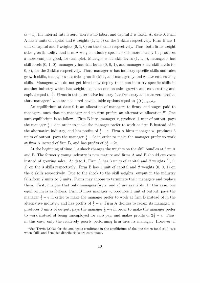
At the beginning of time 1, a shock changes the weights on the skill bundles at firm A

and B. The formerly young industry is now mature and firms A and B should cut costs

instead of growing sales. At date 1, Firm A has 3 units of capital and θ weights (1, 0,

1) on the 3 skills respectively. Firm B has 1 unit of capital and θ weights (0, 0, 1) on

the 3 skills respectively. Due to the shock to the skill weights, output in the industry

falls from 7 units to 3 units. Firms may choose to terminate their managers and replace

them. First, imagine that only managers (w, x, and y) are available. In this case, one

equilibrium is as follows: Firm B hires manager y, produces 1 unit of output, pays the

manager 12

+ ε in order to make the manager prefer to work at firm B instead of in the

alternative industry, and has profits of 12− ε. Firm A decides to retain its manager, w,

produces 3 units of output, pays the manager 12+ ε in order to make the manager prefer

to work instead of being unemployed for zero pay, and makes profits of 212− ε. Thus,

in this case, only the relatively poorly performing firm fires its manager. However, if

10See Tervio (2008) for the analogous conditions in the equilibrium of the one-dimensional skill casewhen skills and firm size distributions are continuous.

10

manager z is available, a candidate equilibrium is: Firm B hires manager y, produces

1 unit of output, pays the manager 12

+ ε in order to make the manager prefer to work

at firm B instead of in the alternative industry, and has profits of 12− ε. Firm A hires

manager z, produces 9 units of output, pays the manager 212

+ 2ε in order to make the

manager prefer to work at firm A instead of firm B and makes profits of 612− 2ε. Thus,

the industry shock may cause both firms to turn over their CEO’s.

Firms will not want to pay for skills they do not find valuable, so when a shock

changes skill weights they are likely to look outside the industry, where these new skills

have been previously productively deployed, for their replacement. Notice also that if

the outside option of deploying general skills in other industries is higher than that of

deploying industry specific skills, the outsiders will tend to be more highly paid relative

to their contribution to output. In the example, consider firm A’s choice of replacement.

To dominate the existing manager, the outsider replacement needs to be able to generate

considerably higher output since all of that output is generated by skills with positive

market prices. As a result, the firm will require much higher output under the new

manager in order to be able to pay the manager the higher required wage and still

increase profits. Thus, when an outsider is hired, output increases significantly and so

does CEO compensation.

2.2 Two Industry Economy

The basic assignment model of Sattinger (1979), Tervio (2008), and Gabaix and Landier

(2008) is built upon the following three simplifying assumptions: First, skills and firm

characteristics are one-dimensional (managers have talent and firms have a size), second,

the distributions of talent and firm size are continuous, and third, firm size and talent

are complements. Assuming skills have only one dimension significantly simplifies the

analysis because wages do not depend on the joint distributions of managerial skills and

firm skill weights. However, if one chooses the distributions carefully, and adopts the

assumptions that skill distributions and firm skill weights are continuous and firm skill

weights and managerial skill levels are complementary, then the analytical techniques

used in Tervio (2008) can be applied to solve for equilibrium wage and profit profiles.

For example, one could assume that general (priced) skills and skill weights are mutu-

ally exclusive. In this case, the demand for a particular manager depends only on one

priced characteristic. Essentially, the model becomes one with separate markets for each

11

dimension of CEO talent. We will not assume that skill weights are mutually exclusive,

for reasons discussed below, but it is a useful starting point for thinking about a multi-

industry, multi-dimensional skill model. We will, however, make convenient assumptions

to reduce the complexity of firm and managerial outside options.

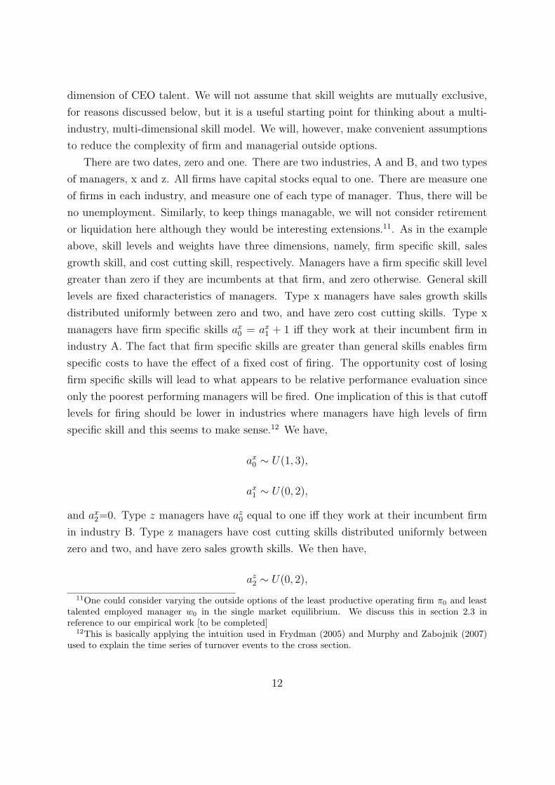
There are two dates, zero and one. There are two industries, A and B, and two types

of managers, x and z. All firms have capital stocks equal to one. There are measure one

of firms in each industry, and measure one of each type of manager. Thus, there will be

no unemployment. Similarly, to keep things managable, we will not consider retirement

or liquidation here although they would be interesting extensions.11. As in the example

above, skill levels and weights have three dimensions, namely, firm specific skill, sales

growth skill, and cost cutting skill, respectively. Managers have a firm specific skill level

greater than zero if they are incumbents at that firm, and zero otherwise. General skill

levels are fixed characteristics of managers. Type x managers have sales growth skills

distributed uniformly between zero and two, and have zero cost cutting skills. Type x

managers have firm specific skills ax0 = ax

1 + 1 iff they work at their incumbent firm in

industry A. The fact that firm specific skills are greater than general skills enables firm

specific costs to have the effect of a fixed cost of firing. The opportunity cost of losing

firm specific skills will lead to what appears to be relative performance evaluation since

only the poorest performing managers will be fired. One implication of this is that cutoff

levels for firing should be lower in industries where managers have high levels of firm

specific skill and this seems to make sense.12 We have,

ax0 ∼ U(1, 3),

ax1 ∼ U(0, 2),

and ax2=0. Type z managers have az

0 equal to one iff they work at their incumbent firm

in industry B. Type z managers have cost cutting skills distributed uniformly between

zero and two, and have zero sales growth skills. We then have,

az2 ∼ U(0, 2),

11One could consider varying the outside options of the least productive operating firm π0 and leasttalented employed manager w0 in the single market equilibrium. We discuss this in section 2.3 inreference to our empirical work [to be completed]

12This is basically applying the intuition used in Frydman (2005) and Murphy and Zabojnik (2007)used to explain the time series of turnover events to the cross section.

12

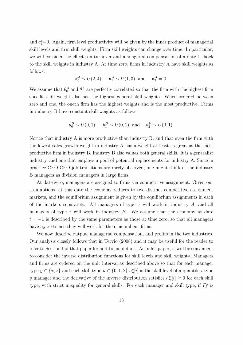
and az1=0. Again, firm level productivity will be given by the inner product of managerial

skill levels and firm skill weights. Firm skill weights can change over time. In particular,

we will consider the effects on turnover and managerial compensation of a date 1 shock

to the skill weights in industry A. At time zero, firms in industry A have skill weights as

follows:

θA0 ∼ U(2, 4), θA

1 ∼ U(1, 3), and θA2 = 0.

We assume that θA0 and θA

1 are perfectly correlated so that the firm with the highest firm

specific skill weight also has the highest general skill weights. When ordered between

zero and one, the oneth firm has the highest weights and is the most productive. Firms

in industry B have constant skill weights as follows:

θB0 ∼ U(0, 1), θB

1 ∼ U(0, 1), and θB2 ∼ U(0, 1).

Notice that industry A is more productive than industry B, and that even the firm with

the lowest sales growth weight in industry A has a weight at least as great as the most

productive firm in industry B. Industry B also values both general skills. It is a generalist

industry, and one that employs a pool of potential replacements for industry A. Since in

practice CEO-CEO job transitions are rarely observed, one might think of the industry

B managers as division managers in large firms.

At date zero, managers are assigned to firms via competitive assignment. Given our

assumptions, at this date the economy reduces to two distinct competitive assignment

markets, and the equilibrium assignment is given by the equilibrium assignments in each

of the markets separately. All managers of type x will work in industry A, and all

managers of type z will work in industry B. We assume that the economy at date

t = −1 is described by the same parameters as those at time zero, so that all managers

have a0 > 0 since they will work for their incumbent firms.

We now describe output, managerial compensation, and profits in the two industries.

Our analysis closely follows that in Tervio (2008) and it may be useful for the reader to

refer to Section I of that paper for additional details. As in his paper, it will be convenient

to consider the inverse distribution functions for skill levels and skill weights. Managers

and firms are ordered on the unit interval as described above so that for each manager

type y ∈ {x, z} and each skill type n ∈ {0, 1, 2} ayn[i] is the skill level of a quantile i type

y manager and the derivative of the inverse distribution satisfies ay′n [i] ≥ 0 for each skill

type, with strict inequality for general skills. For each manager and skill type, if F ya is

13

the cumulative distribution of a for type y, then the profile of a is given by

ay[i] = ay s.t. F ya (a) = i.

Basically, ay[i] gives the ability level of the ith type y manager. The inverse dis-

tribution functions for firms’ skill weights are defined analogously for industries A and

B.

In each industry, the equilibrium assignment must satisfy two types of constraints.

First, the sorting constraints state that each firm must prefer hiring its manager at their

equilibrium wage to hiring any alternative manager at that replacement manager’s equi-

librium wage. Second, the participation constraints state that all firms and individuals

must earn their outside option for opportunities outside of industries A and B. In our

economy, we set these outside options to be equal to zero, and leave the study of vari-

ation in liquidation and retirement options to future research. We have the following

constraints where boldface type is used to denote vectors:

V (ax[i],θA[i])− wx[i] ≥ V (ax[j],θA[i])− wx[j] ∀i, j ∈ [0, 1] SC(i, j) (1)

V (ax[i],θA[i])− wx[i] ≥ 0 ∀i, j ∈ [0, 1] PC θA[i] (2)

wx[i] ≥ 0 PC ax[i] (3)

Analogous sorting constraints must hold across industries, but we ignore them at date

0 since they will not be binding. They will bind for some agents at date 1. Note also

that the only binding sorting constraints within an industry are those which consider

hiring the next best manager. Moreover, since firm specific skills are not valued outside

the firm, and firms in industry A at time zero have θ2 = 0, one only needs to consider

the effects of a1 and θ1. As a result, the date zero economy reduces to two economies of

the type studied in Tervio (2008). Analogous constraints must be satisfied in industry

B which will employ type z managers. The participation constraints will bind for the

lowest ability manager and the lowest productivity firm.

We now solve for wages and profits at time zero. Regrouping the sorting constraints

for types i and i− ε and dividing by ε yields:

V (ax[i],θA[i])− V (ax[i− ε], θA[i])

ε≥ wx[i]− wx[i− ε]

ε.

14

Taking the limit as ε → 0 we get the slope of the wage profile for type x managers:13

wx′[i] = Va(ax[i],θA[i]) · ax′[i].

Finally, integrating, and adding the binding participation constraint yields the wage

profile:

wx[i] = w0 +

∫ i

0

Va(ax[j],θA[j]) · ax′[j] dj

Again, since firm specific skills are not valued outside the firm, and firms in industry A

at time zero have θA2 = 0, to compute wages one only needs to consider the effects of ax

1

and θA1 . Note that the sorting constraints could have been written from the manager’s

perspective, and an analogous profile for profits can be obtained as follows:14

πA[i] = π0 +

∫ i

0

Vθ(ax[j],θA[j]) · θA′[j] dj.

Using the distributions for θA and ax, the definition V (ax[i],θA[i]) = ax[i] · θA[i] kα,

and the fact that k = 1 ∀i, we have that output in industry A is given by:15

V A(i, i) = 1 + 6i + 8i2

wages, or managerial outside options are given by,16

wx(i) = 2i + 2i2

and firm profits are given by17

πA(i) = 2 + 6i + 6i2.

13Note that because of the discontinuity in the value of a0 as managers change firms one technicallycan’t use this argument for firm specific skills. Firm specific skills are unpriced and have a wage of zero.One can think of taking the limit only over the part of V which comes from general skills, and thenadding the output and profits from general skills separately.

14Here again, due to the discontinuity in ax0 across firms, one can integrate over the general skills

contribution to profits and add the contribution of firm specific skills separately.15To compute output, note that output equals θ0(i)a0(i)+ θ1(i)a1(i)+ θ2(i)a2(i) and use the distribu-

tions for skills and skill weights to compute output as a function of i. In particular, note that θA0 = 1+2i,

ax0 = 1 + 2i, θA

1 = 1 + 2i, ax1 = 2i, θA

2 = 0, and ax2 = 0.

16For wages, note that ax1 [j] = 2j so that ax′

1 [j] = 2, and θA1 (j) = 1 + 2j so

∫ 1

0θA1 (j) dj = j + j2.

17For profits from general skills, note that θA1 (j) = 1+2j so θA′

1 (j) = 2 and ax1(j) = 2j so

∫ 1

0ax1(j) dj =

j2.

15

�������

���� ����������

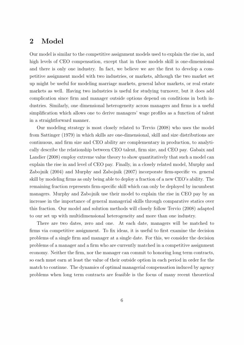
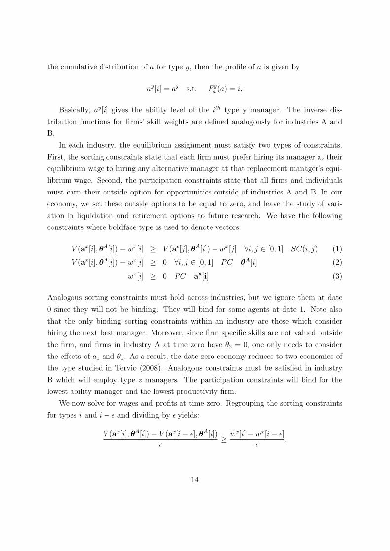
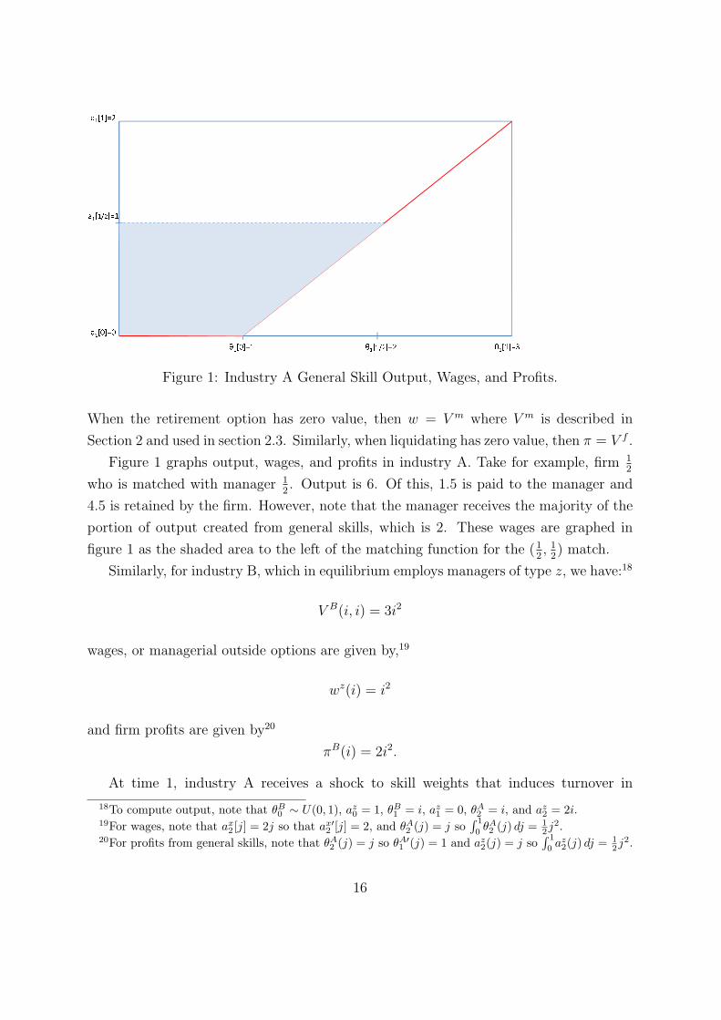
���� ��� ���� ��� �������Figure 1: Industry A General Skill Output, Wages, and Profits.

When the retirement option has zero value, then w = V m where V m is described in

Section 2 and used in section 2.3. Similarly, when liquidating has zero value, then π = V f .

Figure 1 graphs output, wages, and profits in industry A. Take for example, firm 12

who is matched with manager 12. Output is 6. Of this, 1.5 is paid to the manager and

4.5 is retained by the firm. However, note that the manager receives the majority of the

portion of output created from general skills, which is 2. These wages are graphed in

figure 1 as the shaded area to the left of the matching function for the (12, 1

2) match.

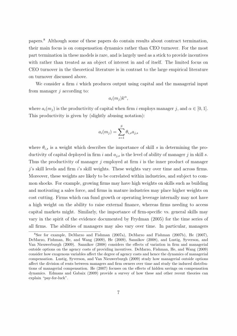
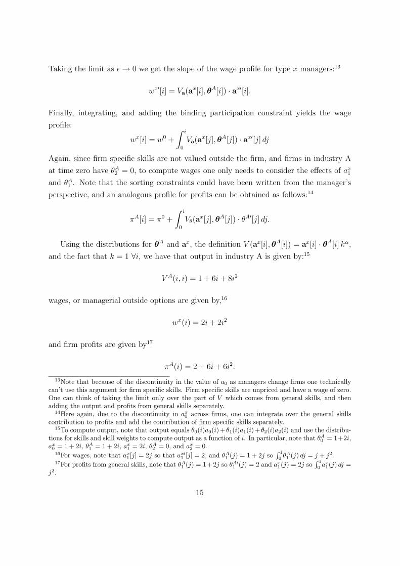
Similarly, for industry B, which in equilibrium employs managers of type z, we have:18

V B(i, i) = 3i2

wages, or managerial outside options are given by,19

wz(i) = i2

and firm profits are given by20

πB(i) = 2i2.

At time 1, industry A receives a shock to skill weights that induces turnover in

18To compute output, note that θB0 ∼ U(0, 1), az

0 = 1, θB1 = i, az

1 = 0, θA2 = i, and az

2 = 2i.19For wages, note that ax

2 [j] = 2j so that ax′2 [j] = 2, and θA

2 (j) = j so∫ 1

0θA2 (j) dj = 1

2j2.20For profits from general skills, note that θA

2 (j) = j so θA′1 (j) = 1 and az

2(j) = j so∫ 1

0az2(j) dj = 1

2j2.

16

�������

���� ����������

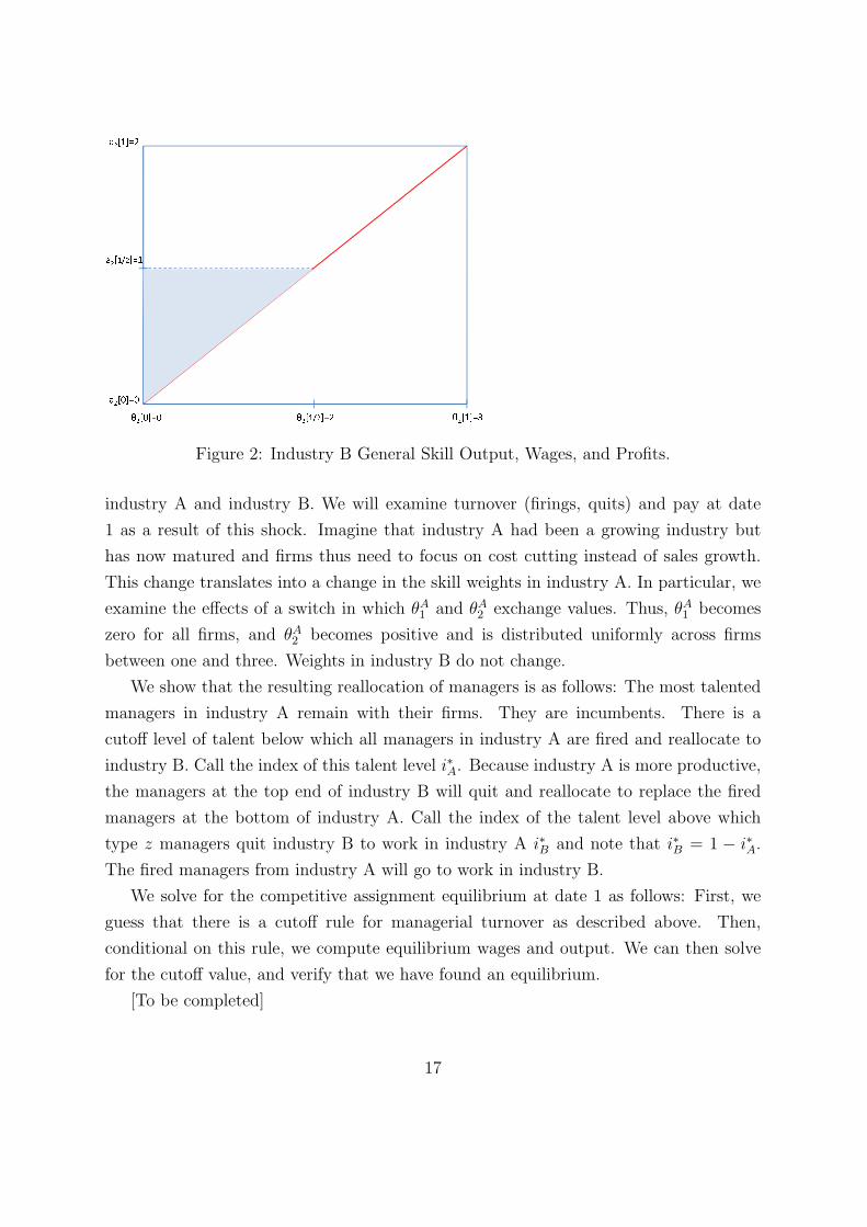
���� ��� ������� �������Figure 2: Industry B General Skill Output, Wages, and Profits.

industry A and industry B. We will examine turnover (firings, quits) and pay at date

1 as a result of this shock. Imagine that industry A had been a growing industry but

has now matured and firms thus need to focus on cost cutting instead of sales growth.

This change translates into a change in the skill weights in industry A. In particular, we

examine the effects of a switch in which θA1 and θA

2 exchange values. Thus, θA1 becomes

zero for all firms, and θA2 becomes positive and is distributed uniformly across firms

between one and three. Weights in industry B do not change.

We show that the resulting reallocation of managers is as follows: The most talented

managers in industry A remain with their firms. They are incumbents. There is a

cutoff level of talent below which all managers in industry A are fired and reallocate to

industry B. Call the index of this talent level i∗A. Because industry A is more productive,

the managers at the top end of industry B will quit and reallocate to replace the fired

managers at the bottom of industry A. Call the index of the talent level above which

type z managers quit industry B to work in industry A i∗B and note that i∗B = 1 − i∗A.

The fired managers from industry A will go to work in industry B.

We solve for the competitive assignment equilibrium at date 1 as follows: First, we

guess that there is a cutoff rule for managerial turnover as described above. Then,

conditional on this rule, we compute equilibrium wages and output. We can then solve

for the cutoff value, and verify that we have found an equilibrium.

[To be completed]

17

2.3 Discussion

Considering again the general model, there are several channels through which changes

in exogenous variables such as industry conditions might drive total surplus below zero

and thereby drive CEO turnover. Throughout the description of the model we used

simple notation and suppressed the dependence of skill weights, skill prices, the pool

of replacement managers, the value of retirement and liquidation and the productivity

of capital on industry conditions. However, we think that such conditions likely affect

all of these variables. Consider first the potential effects of a deterioration in industry

conditions on the outside option of the firm. As the industry declines, the optimal

managerial skill bundle may change as it did in our example, for instance to more heavily

weigh cost cutting or the ability to access capital markets. Firms may find it profitable

to fire incumbent managers and hire managers with the newly more desirable bundle.

Thus, a model like the one described can generate more forced turnover or firings when

industry conditions are poor under what seem to be reasonable assumptions about the

relationship between the firm’s outside option and what is going on in the industry. Next,

consider how industry conditions might change the outside option of the manager and

lead to managers quitting for better jobs or retiring. Changes in industry conditions can

change skill prices and lead the manager to leave for greener pastures. Finally, industry

conditions can change the relative value of retirement through affecting the disutility of

work and the value of retirement compensation packages.

Industry conditions affect turnover in the competitive assignment model and in the

data. However, firm relative to industry performance is the most important predictor of

observing an instance of forced turnover, both in our data and in that of previous studies.

The finding that RPE apparently has such a large empirical contribution to turnover

seems to suggest that there is quite a bit of private information and/or learning about

CEO ability. However, note that even without private information one might observe

what would appear to be RPE driven turnover in data generated by a model like the one

described. In our example, depending on available managers’ skills, it is possible that

only the poorly performing firm would choose to replace its manager after the industry

shock. Thus, finding that RPE drives turnover does not show that boards are effectively

dealing with a problem of asymmetric information. The empirical relationship between

poor performance and turnover may simply be due to variation in the importance or level

of firm or industry specific skills which may lead only the poorest performing firms to seek

replacements. Alternatively, there may be other fixed costs of replacement which would

18

also lead to performance thresholds for firing managers. On the other hand, the converse

is also true. Even if the data did not find such strong support for RPE, one could still

not conclude that boards were not using RPE to gauge talent and effort if other drivers

for turnover also exist. We believe that both learning about unobservable managerial

skills, and shocks to demands for observable talents, are important contributors to CEO

turnover.

Explicitly considering the outside options of both managers and firms in our com-

petitive assignment framework illustrates another, perhaps surprising feature of such a

model which is also consistent with the data. In the model, as in the data, it is actually

quite difficult to label a separation as a “quit” or “fire”. Since empirically separations

are typically labeled as quits or fires by utilizing news stories as we do here, one might

think that the large fraction of turnovers which can neither be labeled as quits or fires

are simply misclassified due to lack of information. One might think that if one had

perfect data, that all separations should be able to be labeled one way or the other.

However, even in data generated by the model, quite reasonable theoretical definitions

of quits and firings would imply that for a large fraction of separations, the agent who

initiated the separation is ambiguous. Separations occur when the total surplus from the

current match is negative. As discussed, this can occur for many reasons on the part of

the firm and the manager, both of whose outside options vary over time, or it can be that

the total value of the match declines. Furthermore, the outside options of the firm and

the manager, as well as the value created by the match depend on the same variables,

namely, skill weights and prices.

We discuss this ambiguity in the context of one specific definition of “quits” vs. “fires”

but note that the model permits others. We introduce time subscripts and suppress

individual agent subscripts to define a separation as follows:

Definition 1 A separation occurs in the current period when a match satisfies the

following two conditions:

Condition 1 Vt − V mt − V f

t < 0

and

Condition 2 Vt−1 − V mt−1 − V f

t−1 > 0.

Now, consider defining a separation as initiated by one agent (either the manager or

the firm) if that agent would choose to remain in the match with the current match value

19

and the current outside option of the other agent, but with their own lagged outside

option. This separation must satisfy conditions 1 and 2 as well as either

Condition 3 (Q) Vt − V mt−1 − V f

t > 0

if the separation is a quit, and

Condition 4 (F) Vt − V mt − V f

t−1 > 0

if the separation is a fire. Note that conditions 1 and Q together simply say that V mt >

V mt−1, while conditions 1 and F together simply say that V f

t > V ft−1. These two inequalities

are not mutually exclusive, so clearly many separations would be unclassified under this

definition. We can, however, refine this definition further.

Add to the definition above that the initiating agent would not want to remain in

the match even given the current match value, that agent’s current outside option, and

the other agent’s lagged outside option. If conditions Q and F are associated with quits

and fires, these new conditions basically state that quits must also not be firings, and

likewise firings must also not be quits. In other words, they require that the separation

also satisfy

Condition 5 (¬F) Vt − V mt − V f

t−1 < 0

if the separation is a quit, and

Condition 6 (¬Q) Vt − V mt−1 − V f

t < 0

if the separation is a fire.

Then, a quit can be defined as a separation which satisfies Q and ¬F. Combining

these two conditions, and condition 1 with condition Q yields the following definition of

a quit:

Definition 2 A separation is a quit if V mt > V m

t−1 and V mt − V m

t−1 > V ft − V f

t−1.

Similarly, a fire can be defined as a separation which satisfies F and ¬Q. Combining

these two conditions, and condition 1 with condition F yields the following definition of

a firing:

Definition 3 A separation is a fire if V ft > V f

t−1 and V ft − V f

t−1 > V mt − V m

t−1.

20

Even these very loose definitions permit separations that cannot be classified in cases in

which the total value of the match drives the surplus negative and outside options remain

unchanged. More strict definitions of quits and fires, such as the one given by conditions

Q and F only, or requiring a quit to satisfy V mt > V m

t−1 and V ft ≤ V f

t−1 and requiring a fire

to satisfy V ft > V f

t−1 and V mt ≤ V m

t−1, would lead to even more ambiguous separations.

However, note that in the model, as in the data, the type of replacement manager, and

the compensation of that manager, would yield additional information about the type of

separation observed.

3 Data

We use four main sources of data: Execucomp for the name and compensation of the

CEOs of 2779 publicly traded companies during 1992-2006, CRSP/Compustat for stock

returns and accounting data for these firms, the industries they belong to, and the market

in general, the Bureau of Economic Analysis for industry and aggregate data (referring

to both public and private firms), and Factiva for news stories published in a three-year

window around CEOs departures. The information in Factiva allows us to determine the

reason why a CEO left and to identify where the replacement CEO came from.21

We identify 2068 instances where a CEO was replaced, and for which we know both

the reason for the incumbent’s departure, as well as where the new CEO came from. Of

all replacements, 613 (29.7%) are the result of a planned retirement decision, announced

at least six months prior to the actual departure date, or of a health-related reason.

Another 323 (15.6%) replacements are instances where the incumbent CEO was forced

out, according to newspaper stories related to the departure. The remaining 1132 (54.7%)

cases are those that do not fit in any of these two categories – retirements or firings –

and thus we will label them unclassified departures. These events include instances

where the incumbent voluntarily left the firm, and therefore we also refer to them as

potential quits. Since these unclassified departures are the residual category, one might

expect them to behave like a weighted average of retirements and forced turnovers. This

is true for some empirical relationships (for example the relationship between relative

firm performance and the likelihood of turnover), but unclassified departures have some

21We are grateful to Dirk Jenter for providing us with the data in Jenter and Kanaan (2006) regardingwhether or not a CEO was fired or chose to retire. We used those data to fill in some of the missingobservations for which our Factiva search was not fruitful.

21

distinct characteristics also. We discuss this more in section 4, but, for example, they have

the strongest negative relationship of all turnover types with contemporaneous market

returns.

Our definition of departure type is different from the algorithm described in Par-

rino (1997) and followed by several other papers, in two significant ways. First, and

most important, the extant literature on turnover identifies just two types of departures:

forced and unforced (the latter including retirements). However, since an employment

relationship is the result of a two-sided matching process that depends on the conditions

in the executive labor market, we allow for turnover to happen for three reasons: the

firm chooses to terminate the match, the CEO chooses to terminate the match but is still

active in the executive labor market, or the CEO leaves the executive labor market for

exogenous reasons such as age and health. These three types of departure have different

theoretical reasons and will be predicted by different variables in the empirical analysis.

Second, unlike Parrino (1997), we do not condition on the incumbent CEO’s age to

define a departure as forced or not. Parrino (1997) classifies as forced departures all

cases where the CEO is younger than 60, and (1) related news stories do not report

the reason for departure as involving death, poor health or the acceptance of another

job, or (2) the firm reports the departure as a retirement, but does so less than six

months before succession. We believe that it is possible that in some of these instances

managers voluntarily quit the job – they were not fired, nor did they choose to leave

the executive labor market (i.e. retire.) Hence, while in papers using the Parrino (1997)

algorithm the age of the departing CEO is a significant and negative predictor of forced

turnover because of the way forced turnovers are defined, in our analysis this mechanical

relationship does not exist.

4 Empirical Results

The three novel theoretical predictions that we will test empirically are as follows:

(H1) When industry conditions deteriorate, forced turnover and voluntary quits are

more likely to occur.

(H2) When industry conditions deteriorate, replacement CEOs are more likely to have

skills different from those of departing CEOs.

(H3) The pay of CEOs reflects the market price of their skill bundles.

22

In line with these predictions, the empirical evidence we document indicates that the

type of CEO departure, as well as the type of CEO hired as a replacement and their pay

depend strongly on the firm’s need for strategy change and on the outside option of both

the firm and the CEO.

In the analysis we build on the findings of a large empirical literature on CEO

turnover. Typically in this literature, either the firm’s stock return or the firm’s re-

turn on assets (ROA), adjusted for industry performance, have been used to predict

CEO turnover, and forced turnover in particular. For instance, Gibbons and Murphy

(1990), Murphy (1999), Jenter and Kanaan (2006) and Kaplan and Minton (2006) use

stock returns, while ROA (typically by itself and not in addition to the stock return)

is used in Barro and Barro (1990), Parrino (1997), Huson, Parrino, and Starks (2001),

and Huson, Malatesta, and Parrino (2004). The evidence in these papers indicates that

relative performance evaluation (Holmstrom (1982)) is used to determine whether a CEO

is fired22 or not: if the firm’s performance (measured as stock return or ROA) relative to

the industry is higher, the probability of the CEO being forced out is lower.

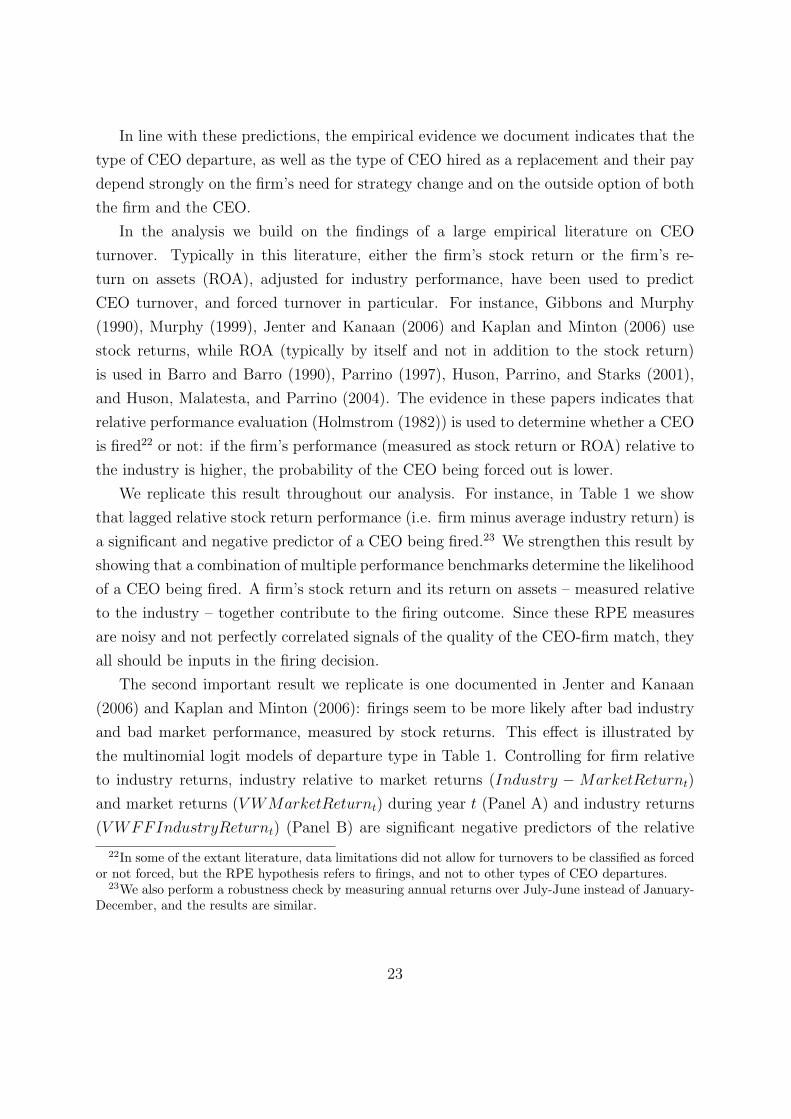
We replicate this result throughout our analysis. For instance, in Table 1 we show

that lagged relative stock return performance (i.e. firm minus average industry return) is

a significant and negative predictor of a CEO being fired.23 We strengthen this result by

showing that a combination of multiple performance benchmarks determine the likelihood

of a CEO being fired. A firm’s stock return and its return on assets – measured relative

to the industry – together contribute to the firing outcome. Since these RPE measures

are noisy and not perfectly correlated signals of the quality of the CEO-firm match, they

all should be inputs in the firing decision.

The second important result we replicate is one documented in Jenter and Kanaan

(2006) and Kaplan and Minton (2006): firings seem to be more likely after bad industry

and bad market performance, measured by stock returns. This effect is illustrated by

the multinomial logit models of departure type in Table 1. Controlling for firm relative

to industry returns, industry relative to market returns (Industry − MarketReturnt)

and market returns (V WMarketReturnt) during year t (Panel A) and industry returns

(V WFFIndustryReturnt) (Panel B) are significant negative predictors of the relative

22In some of the extant literature, data limitations did not allow for turnovers to be classified as forcedor not forced, but the RPE hypothesis refers to firings, and not to other types of CEO departures.

23We also perform a robustness check by measuring annual returns over July-June instead of January-December, and the results are similar.

23

likelihood of the CEO being forced out versus there being no turnover during year t+1.24

Although these results have been documented previously, we provide a unique inter-

pretation here. As our competitive assignment model suggests, industry conditions affect

the CEO-firm match surplus and thus drive turnovers. We will now turn to the novel

empirical findings we document, in light of the predictions of our theoretical framework.

4.1 Match dissolution

The first novel hypothesis of the competitive assignment framework that we test, (H1),

states that when industry conditions deteriorate, forced turnover and voluntary quits are

more likely to occur.

We first observe that turnover of all types, and forced turnover in particular, are

relatively concentrated. Using the Fama French 48 industry classification system, we

find that 50% of all instances of forced turnover occur in just seven industries: Business

Services, Computers, Retail, Utilities, Chips, Machinery and Drugs. Overall turnover

is also concentrated in several industries, although less so than forced turnover. The

top 5% of 608 industry-year bins that our observations belong to account for 22% of all

turnover events, and for 35% of forced turnover. Since these CEO-firm match dissolution

events are not uniformly distributed across industries and over time, we investigate what

specific industry conditions may drive turnover.

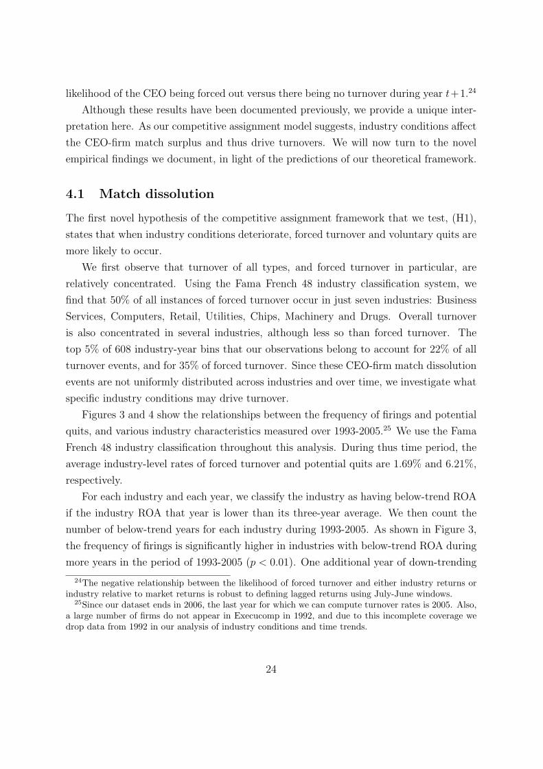
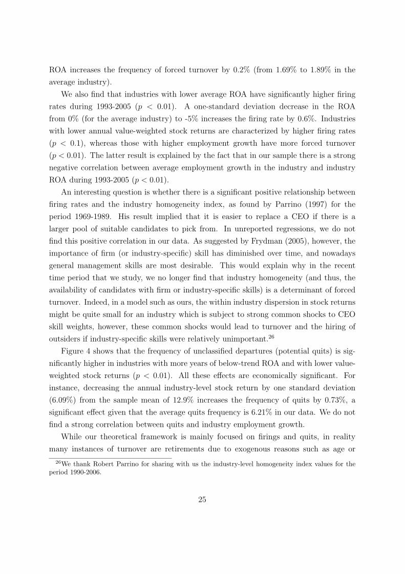
Figures 3 and 4 show the relationships between the frequency of firings and potential

quits, and various industry characteristics measured over 1993-2005.25 We use the Fama

French 48 industry classification throughout this analysis. During thus time period, the

average industry-level rates of forced turnover and potential quits are 1.69% and 6.21%,

respectively.

For each industry and each year, we classify the industry as having below-trend ROA

if the industry ROA that year is lower than its three-year average. We then count the

number of below-trend years for each industry during 1993-2005. As shown in Figure 3,

the frequency of firings is significantly higher in industries with below-trend ROA during

more years in the period of 1993-2005 (p < 0.01). One additional year of down-trending

24The negative relationship between the likelihood of forced turnover and either industry returns orindustry relative to market returns is robust to defining lagged returns using July-June windows.

25Since our dataset ends in 2006, the last year for which we can compute turnover rates is 2005. Also,a large number of firms do not appear in Execucomp in 1992, and due to this incomplete coverage wedrop data from 1992 in our analysis of industry conditions and time trends.

24

ROA increases the frequency of forced turnover by 0.2% (from 1.69% to 1.89% in the

average industry).

We also find that industries with lower average ROA have significantly higher firing

rates during 1993-2005 (p < 0.01). A one-standard deviation decrease in the ROA

from 0% (for the average industry) to -5% increases the firing rate by 0.6%. Industries

with lower annual value-weighted stock returns are characterized by higher firing rates

(p < 0.1), whereas those with higher employment growth have more forced turnover

(p < 0.01). The latter result is explained by the fact that in our sample there is a strong

negative correlation between average employment growth in the industry and industry

ROA during 1993-2005 (p < 0.01).

An interesting question is whether there is a significant positive relationship between

firing rates and the industry homogeneity index, as found by Parrino (1997) for the

period 1969-1989. His result implied that it is easier to replace a CEO if there is a

larger pool of suitable candidates to pick from. In unreported regressions, we do not

find this positive correlation in our data. As suggested by Frydman (2005), however, the

importance of firm (or industry-specific) skill has diminished over time, and nowadays

general management skills are most desirable. This would explain why in the recent

time period that we study, we no longer find that industry homogeneity (and thus, the

availability of candidates with firm or industry-specific skills) is a determinant of forced

turnover. Indeed, in a model such as ours, the within industry dispersion in stock returns

might be quite small for an industry which is subject to strong common shocks to CEO

skill weights, however, these common shocks would lead to turnover and the hiring of

outsiders if industry-specific skills were relatively unimportant.26

Figure 4 shows that the frequency of unclassified departures (potential quits) is sig-

nificantly higher in industries with more years of below-trend ROA and with lower value-

weighted stock returns (p < 0.01). All these effects are economically significant. For

instance, decreasing the annual industry-level stock return by one standard deviation

(6.09%) from the sample mean of 12.9% increases the frequency of quits by 0.73%, a

significant effect given that the average quits frequency is 6.21% in our data. We do not

find a strong correlation between quits and industry employment growth.

While our theoretical framework is mainly focused on firings and quits, in reality

many instances of turnover are retirements due to exogenous reasons such as age or

26We thank Robert Parrino for sharing with us the industry-level homogeneity index values for theperiod 1990-2006.

25

health. In our data, the average industry-level rate of retirements is 3.32%.27 As shown

in Figure 5, industry characteristics tend not to be significant drivers of the retirement

frequency. The one marginally significant result is that the frequency of retirements

is higher in industries with lower employment growth (p < 0.1). This indicates that

retirement decisions may not be exogenous to the firm or aggregate conditions, as one

might think. CEOs have some leeway in when they choose to retire, and may do so where

their outside option is better than the payoff from staying with the firm. It is possible

that retention payoffs are relatively less attractive in industries with lower employment

growth, if empire-building is part of these payoffs.

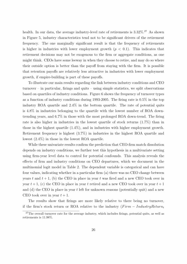
To illustrate our main results regarding the link between industry conditions and CEO

turnover – in particular, firings and quits – using simple statistics, we split observations

based on quartiles of industry conditions. Figure 6 shows the frequency of turnover types

as a function of industry conditions during 1993-2005. The firing rate is 0.5% in the top

industry ROA quartile and 2.4% in the bottom quartile. The rate of potential quits

is 4.8% in industries belonging to the quartile with the lowest number of ROA down-

trending years, and 6.7% in those with the most prolonged ROA down-trend. The firing

rate is also higher in industries in the lowest quartile of stock returns (1.7%) than in

those in the highest quartile (1.4%), and in industries with higher employment growth.

Retirement frequency is highest (3.7%) in industries in the highest ROA quartile and

lowest (2.4%) in those in the lowest ROA quartile.

While these univariate results confirm the prediction that CEO-firm match dissolution

depends on industry conditions, we further test this hypothesis in a multivariate setting

using firm-year level data to control for potential confounds. This analysis reveals the

effects of firm and industry conditions on CEO departures, which we document in the

multinomial logit model in Table 2. The dependent variable is categorical and can have

four values, indicating whether in a particular firm (a) there was no CEO change between

years t and t + 1, (b) the CEO in place in year t was fired and a new CEO took over in

year t + 1, (c) the CEO in place in year t retired and a new CEO took over in year t + 1

and (d) the CEO in place in year t left for unknown reasons (potentially quit) and a new

CEO took over in year t + 1.

The results show that firings are more likely relative to there being no turnover,

if the firm’s stock return or ROA relative to the industry (Firm − IndustryReturnt

27The overall turnover rate for the average industry, which includes firings, potential quits, as well asretirements is 11.98%.

26

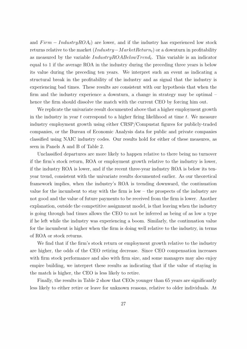
and Firm − IndustryROAt) are lower, and if the industry has experienced low stock

returns relative to the market (Industry−MarketReturnt) or a downturn in profitability

as measured by the variable IndustryROABelowTrendt. This variable is an indicator

equal to 1 if the average ROA in the industry during the preceding three years is below

its value during the preceding ten years. We interpret such an event as indicating a

structural break in the profitability of the industry and as signal that the industry is

experiencing bad times. These results are consistent with our hypothesis that when the

firm and the industry experience a downturn, a change in strategy may be optimal –

hence the firm should dissolve the match with the current CEO by forcing him out.

We replicate the univariate result documented above that a higher employment growth

in the industry in year t correspond to a higher firing likelihood at time t. We measure

industry employment growth using either CRSP/Compustat figures for publicly-traded

companies, or the Bureau of Economic Analysis data for public and private companies

classified using NAIC industry codes. Our results hold for either of these measures, as

seen in Panels A and B of Table 2.

Unclassified departures are more likely to happen relative to there being no turnover

if the firm’s stock return, ROA or employment growth relative to the industry is lower,

if the industry ROA is lower, and if the recent three-year industry ROA is below its ten-

year trend, consistent with the univariate results documented earlier. As our theoretical

framework implies, when the industry’s ROA is trending downward, the continuation

value for the incumbent to stay with the firm is low – the prospects of the industry are

not good and the value of future payments to be received from the firm is lower. Another

explanation, outside the competitive assignment model, is that leaving when the industry

is going through bad times allows the CEO to not be inferred as being of as low a type

if he left while the industry was experiencing a boom. Similarly, the continuation value

for the incumbent is higher when the firm is doing well relative to the industry, in terms

of ROA or stock returns.

We find that if the firm’s stock return or employment growth relative to the industry

are higher, the odds of the CEO retiring decrease. Since CEO compensation increases

with firm stock performance and also with firm size, and some managers may also enjoy

empire building, we interpret these results as indicating that if the value of staying in

the match is higher, the CEO is less likely to retire.

Finally, the results in Table 2 show that CEOs younger than 65 years are significantly

less likely to either retire or leave for unknown reasons, relative to older individuals. At

27

the same time, the likelihood of being fired relative to continuing as a CEO does not

depend on the executive’s age.

4.2 Match formation

In this section we test the second hypothesis, (H2), which states that when industry

conditions deteriorate, replacement CEOs are more likely to have skills different from

those of departing CEOs.

We first document general patterns in the types of replacements hired during 1993-

2005. The frequency of replacements by company insiders has decreased over time from

70% in 1993 to 59.5% in 2005, supporting the argument that general management skills

are now relatively more valuable than firm-specific skills compared to earlier periods (Fry-

dman (2005)). Also, the frequency of replacements by individuals coming from privately-

held firms has increased over time, from 1.75% in 1993 to 5.40% in 2005.

In line with our hypothesis that matches are formed based on the fit of the CEO’s

skill set with the company’s needs, we find evidence suggesting that companies going

through difficult times, either because of idiosyncratic reasons or because of industry

conditions, are more likely to hire replacement CEOs with a different background than

the incumbent executive.

We find that company outsiders are more likely to be brought in after a firing or after a

voluntary departure of the incumbent, which tend to occur when the firm or the industry

experience difficult times, than after a retirement. Moreover, most of these outsiders

are from a different industry according to the Fama French 48 industry classification

system.28

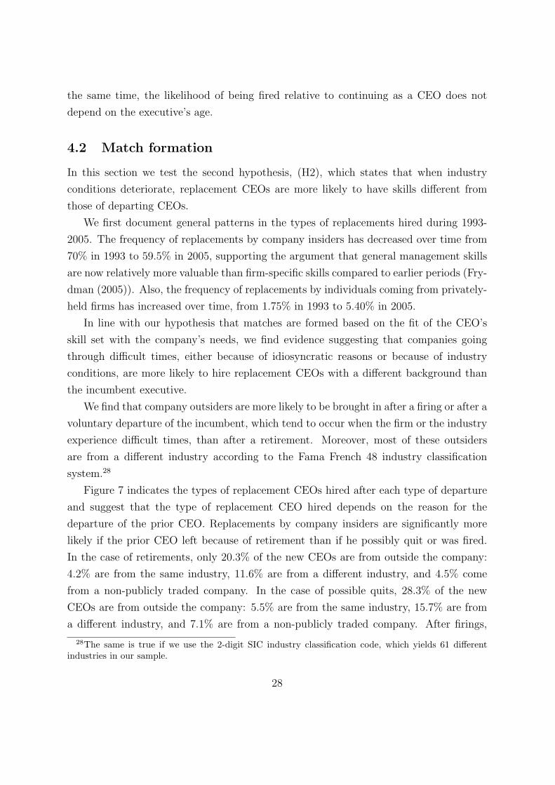
Figure 7 indicates the types of replacement CEOs hired after each type of departure

and suggest that the type of replacement CEO hired depends on the reason for the

departure of the prior CEO. Replacements by company insiders are significantly more

likely if the prior CEO left because of retirement than if he possibly quit or was fired.

In the case of retirements, only 20.3% of the new CEOs are from outside the company:

4.2% are from the same industry, 11.6% are from a different industry, and 4.5% come

from a non-publicly traded company. In the case of possible quits, 28.3% of the new

CEOs are from outside the company: 5.5% are from the same industry, 15.7% are from

a different industry, and 7.1% are from a non-publicly traded company. After firings,

28The same is true if we use the 2-digit SIC industry classification code, which yields 61 differentindustries in our sample.

28

37.8% of replacements are company outsiders: 9.1% are from the same industry, 21.2%

from another industry, and 7.5% from a non-publicly traded company.

We check the robustness of these results by estimating a multinomial logit model

of the relative likelihood of various types of replacement CEOs as function of the prior

CEO’s departure reason, and industry fixed-effects. The results are shown in Table 3

and confirm the unconditional findings.

To get more direct evidence that industry conditions matter for the type of replace-

ment CEO hired, we split the firm-year observations into those belonging to industries

with below-average and above-average ROA during 1993-2005. To keep the analysis sim-

ple, we bundle together all three types of replacement CEOs from outside the company,

and refer to these individuals as “outsiders”. Replacement CEOs hired from within the

firm are referred to as “insiders”.

Figure 8 shows that the number and frequency of turnover events for low and high

ROA industries, and for each departure reason and replacement type. In low ROA

industries there are more instances of firings and unclassified departures (possible quits)

than in high ROA industries, and in such instances it is more likely that an outsider

will be brought in, relative to similar instances in high ROA industries. For instance,

in high ROA industries there were 122 instances were the incumbent was fired and in

36% of these cases, he was replaced by an outsider. In low ROA industries there were

185 firings, and 39% of these instances led to an outside hire. Similarly, in high ROA

industries there were 518 instances of possible quits, and 25% of these were followed by

an outside hire. In low ROA industries, there were 619 instances of possible quits, and

in 32% of these cases an outsider was brought in.

We interpret these patterns as evidence that the more likely it is that the incumbent

CEO-firm match is suboptimal, the more likely it is for the firm to bring in a replacement

CEO with a different background and expertise than a company insider. This evidence

is consistent with the finding documented by Allgood and Farrell (2003) that best firm-

CEO matches tend to occur when inside CEOs follow previous CEOs who quit, and when

outside CEOs follow previous CEOs who are dismissed.

To see whether these univariate results are robust, we estimate a multivariate probit

model for the likelihood that the replacement CEO is an outsider. We allow stock market

and real variables that describe firm and industry conditions to influence this likelihood,

as we did in our analysis of types of CEO departures in Table 2. The results of this

probit model are shown in Table 4.

29

Since we condition on there being turnover and then inquire what type of CEO is

hired, our analysis is different from that in Parrino (1997), where firm-specific perfor-

mance is used to predict what type of CEO is in place, and “no turnover” (i.e. the

incumbent is still CEO) is one of the possible outcomes. The results there indicate that

the likelihood of outside succession, relative to there being no turnover, is negatively

related to industry-adjusted stock returns and ROA. In other words, replacing a CEO,

and doing so with an outsider, happens when the firm is underperforming the industry.

Our evidence complements the result in Parrino (1997) and also shows that industry

conditions matter for the type of CEO hired. We argue that this is because of the effect

of such conditions on the desired management style or skill set.

The results in Table 4 show that the probability of a replacement by an outsider

relative to an insider is higher when the firm’s industry-adjusted stock return and ROA

are lower, a result very much in the spirit of that of Parrino (1997). We also find that a

succession by a company outsider is more likely relative to an inside succession when the

industry ROA is lower, and if the industry has experienced a lower growth in employment.

This pattern holds whether we measure employment using CRSP/Compustat figures that

refer to public companies only, or BEA figures that capture the overall employment in pri-

vate and public companies (reported using the NAIC industry classification). Therefore,

replacements by outsiders seem to be particularly common after poor firm and industry

performance, that is, at times when continuing the same strategy as before may not be

beneficial.

Figure 9 shows the dynamics of firm ROA performance relative to the industry for

all CEO departure reasons and replacement types, to illustrate that these different types

of turnover events happen to firms in different circumstances. Independent of the type

of CEO departure, the firm’s ROA relative to that of the industry is lower prior to the

turnover event in cases where the new CEO is a company outsider, relative to those where

there is no replacement or the new CEO is a company insider. The under-performance

of firms under incumbent CEOs who are eventually replaced by outsiders is greatest in

instances when the incumbent is fired, and smallest in instances when the incumbent’s

departure is due to retirement. Overall, it appears that outside CEOs are brought in to

replace incumbents who are no longer a good match for the firm.

30

4.3 Compensation and CEO skills

The third main hypothesis we test, (H3), states that the pay of CEOs reflects the market

price of their skill bundles. As the model suggests, the pay offered to the new CEO

must compensate him for his forgone outside option. For an individual to decide to take

the CEO job at a firm that is performing poorly, or is in an industry going through

a downturn, he must receive higher compensation than the CEO of a less distressed

firm, as suggested by the example in section 2.1. We find evidence consistent with these

arguments, as shown in Figures 10 to 14 and the regression model in Table 5.

When an outsider is brought in, irrespective of the reason for departure of the prior

CEO, his total pay is higher than that of an insider replacement, a continuing CEO

or the prior CEO (Figure 10). Therefore, since pay does not decrease in the event of

a replacement by an outsider, such events must occur because the outsider’s ability or

quality of match is higher than that of the incumbent, and because the outsider has more

general human capital than the incumbent CEO that can be deployed in other firms or

industries.

The sizable increase in pay of the outsider relative to that of an insider replacement,

a continuing CEO or the prior CEO is driven mostly by the value of the option grants

given to the new CEO who is brought from outside the company (Figure 11) and less so

through bonuses (Figure 13) or other types of pay that exclude salary, bonus or option

grants (Figure 14). Salaries of outsider replacement CEOs are actually lower than those

received by CEOs in these three comparison categories (Figure 12). The highest pay is

received by new CEOs who come in after the prior CEO was fired, with outsiders getting

paid more than insiders. New CEOs from inside the company are paid a similar amount

as continuing CEOs at companies that do not experience turnover.

The regression models in Table 5 yield the same results as univariate findings in

Figures 10 through 14. Controlling for industry and year fixed-effects, as well as firm

market value, we find that the total pay of a new CEO is lowest if he is an insider

replacing a retired incumbent ($0.45 million less than the pay of a continuing CEO), and

highest if he is a company outsider replacing a fired incumbent ($2.5 million more than

the pay of a continuing CEO). Irrespective of the departure reason (retirement, possible

quit, or forced out), the replacement CEO will earn total compensation equal or lower

than continuing CEOs if he is a company insider, but higher than continuing CEOs if he

is a company outsider.

31

5 Conclusion

We consider the link between industry conditions and the CEO labor market in the

context of a competitive assignment model where both the CEO and firm optimize over

the relative value of preserving the match versus pursuing their outside option. In contrast

to a principal-agent framework where only relative performance affects CEO turnover, in

a matching environment both firm and CEO characteristics as well as broader industry

conditions naturally drive turnover events. Although the competitive assignment model

has been used by several authors recently to explain empirical facts about CEO pay, we

are the first to show that such a model can also be used to successfully understand the

dynamics of CEO turnover.

We find empirical support for these ideas using a large dataset we construct describing

turnover events during the period 1992-2006. We collect information regarding both the

reason for the incumbent CEO’s departure and the identity and background of the new

CEO. This information allows us to ascertain with greater precision the reason behind the

turnover event. We study the effect of firm and industry conditions on the likelihood of

turnovers categorized as forced departures, quits or retirements. We similarly document

the determinants of the choice of whether the replacement CEO will be a firm insider or

outsider, and show that type and pay of the new CEO is related to the reason behind

the incumbent’s replacement. Our empirical findings generally match our theoretical

predictions and illustrate that a competitive assignment model can explain the patterns

in observed managerial turnover across industries and over time.

32

References

Allgood, S. and K. A. Farrell (2003). The match between CEO and firm. Journal of

Business 76 (2), 317–341.

Barro, J. R. and R. J. Barro (1990, October). Pay, performance and turnover of bank

CEOs. Journal of Labor Economics 8 (4), 448–481.

Bebchuk, L. and J. Fried (2004). Pay without Performance. Cambridge, MA and Lon-

don, England: Harvard University Press.

Bertrand, M. and A. Schoar (2003, November). Managing with style: The effect of

managers on firm policies. Quarterly Journal of Economics 118 (4), 1169:1208.

DeMarzo, P., M. Fishman, Z. He, and N. Wang (2009). Dynamic agency and the q

theory of investment. Working paper .

DeMarzo, P. M. and M. J. Fishman (2007a, January). Agency and optimal investment

dynamics. Review of Financial Studies 20, 151–188.

DeMarzo, P. M. and M. J. Fishman (2007b, November). Optimal long-term financial

contracting. Review of Financial Studies 20, 2079–2128.

Dicks, D. (2009). Executive Compensation, Incentives, and the Role for Corporate

Governance Regulation. Working paper, UNC .

Edmans, A. and X. Gabaix (2009). Is CEO pay really inefficient? A survey of new

optimal contracting theories. European Financial Management 15 (3), 486–496.

Eisfeldt, A. and A. Rampini (2008). Managerial incentives, capital reallocation, and

the business cycle. Journal of Financial Economics , 177–199.

Frydman, C. (2005). Rising Through the Ranks. The Evolution of the Market for

Corporate Executives, 1936-2003. Harvard University, Working Paper .

Gabaix, X. and A. Landier (2008). Why Has CEO Pay Increased So Much? Quarterly

Journal of Economics 123 (1), 49–100.

Giannetti, M. (2009). Serial CEO incentives and the structure of managerial contracts.

Working paper .

Gibbons, R. and K. J. Murphy (1990, February). Relative performance evaluation for

Chief Executive Officers. Industrial and Labor Relations Review 43 (3. Special issue:

Do Compensation Policies Matter?), 30S–51S.

33

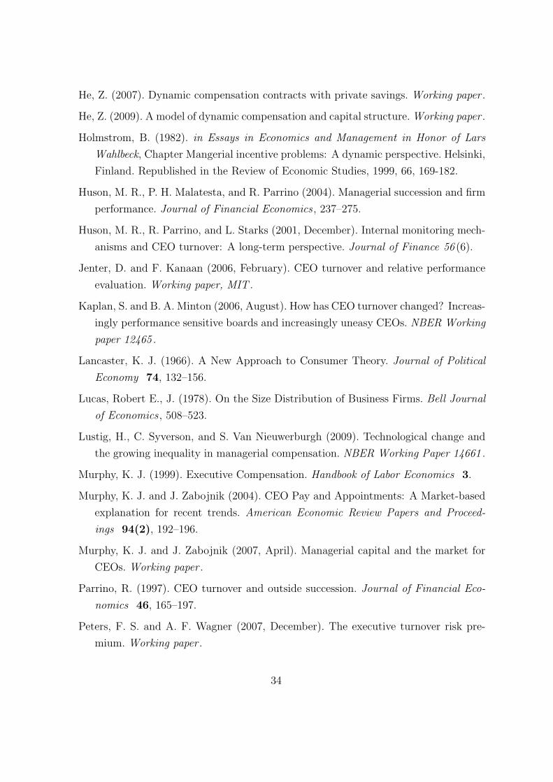
He, Z. (2007). Dynamic compensation contracts with private savings. Working paper .

He, Z. (2009). A model of dynamic compensation and capital structure. Working paper .

Holmstrom, B. (1982). in Essays in Economics and Management in Honor of Lars

Wahlbeck, Chapter Mangerial incentive problems: A dynamic perspective. Helsinki,

Finland. Republished in the Review of Economic Studies, 1999, 66, 169-182.

Huson, M. R., P. H. Malatesta, and R. Parrino (2004). Managerial succession and firm

performance. Journal of Financial Economics , 237–275.

Huson, M. R., R. Parrino, and L. Starks (2001, December). Internal monitoring mech-

anisms and CEO turnover: A long-term perspective. Journal of Finance 56 (6).

Jenter, D. and F. Kanaan (2006, February). CEO turnover and relative performance

evaluation. Working paper, MIT .

Kaplan, S. and B. A. Minton (2006, August). How has CEO turnover changed? Increas-

ingly performance sensitive boards and increasingly uneasy CEOs. NBER Working

paper 12465 .

Lancaster, K. J. (1966). A New Approach to Consumer Theory. Journal of Political

Economy 74, 132–156.

Lucas, Robert E., J. (1978). On the Size Distribution of Business Firms. Bell Journal

of Economics , 508–523.

Lustig, H., C. Syverson, and S. Van Nieuwerburgh (2009). Technological change and

the growing inequality in managerial compensation. NBER Working Paper 14661 .

Murphy, K. J. (1999). Executive Compensation. Handbook of Labor Economics 3.

Murphy, K. J. and J. Zabojnik (2004). CEO Pay and Appointments: A Market-based

explanation for recent trends. American Economic Review Papers and Proceed-

ings 94(2), 192–196.

Murphy, K. J. and J. Zabojnik (2007, April). Managerial capital and the market for

CEOs. Working paper .

Parrino, R. (1997). CEO turnover and outside succession. Journal of Financial Eco-

nomics 46, 165–197.

Peters, F. S. and A. F. Wagner (2007, December). The executive turnover risk pre-

mium. Working paper .

34

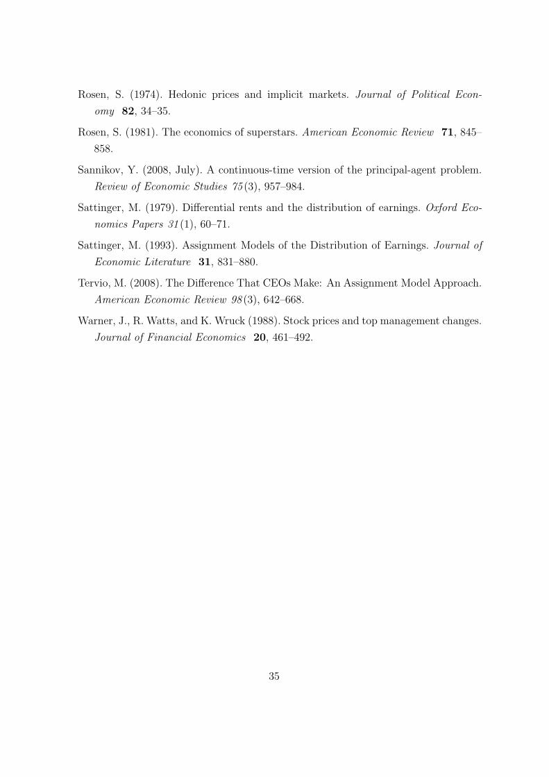
Rosen, S. (1974). Hedonic prices and implicit markets. Journal of Political Econ-

omy 82, 34–35.

Rosen, S. (1981). The economics of superstars. American Economic Review 71, 845–

858.

Sannikov, Y. (2008, July). A continuous-time version of the principal-agent problem.

Review of Economic Studies 75 (3), 957–984.

Sattinger, M. (1979). Differential rents and the distribution of earnings. Oxford Eco-

nomics Papers 31 (1), 60–71.

Sattinger, M. (1993). Assignment Models of the Distribution of Earnings. Journal of

Economic Literature 31, 831–880.

Tervio, M. (2008). The Difference That CEOs Make: An Assignment Model Approach.

American Economic Review 98 (3), 642–668.

Warner, J., R. Watts, and K. Wruck (1988). Stock prices and top management changes.

Journal of Financial Economics 20, 461–492.

35

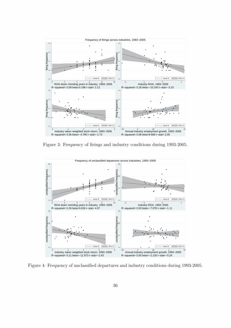
−2

02

46

firin

g fr

eque

ncy

0 2 4 6 8 10

ROA down−trending years in industry, 1993−2005

linear fit 95% CI

R−squared= 0.09 beta=0.198 t−stat= 2.12

−2

02

46

firin

g fr

eque

ncy

−.2 −.1 0 .1

Industry ROA, 1993−2005

linear fit 95% CI

R−squared= 0.18 beta=−10.243 t−stat=−3.23

−2

02

46

firin

g fr

eque

ncy

0 .1 .2 .3 .4

Industry value−weighted stock return, 1993−2005

linear fit 95% CI

R−squared= 0.06 beta=−4.790 t−stat=−1.73

−2

02

46

firin

g fr

eque

ncy

−.05 0 .05 .1 .15

Annual industry employment growth, 1993−2005

linear fit 95% CI

R−squared= 0.08 beta=9.669 t−stat= 2.05

Frequency of firings across industries, 1993−2005

Figure 3: Frequency of firings and industry conditions during 1993-2005.

05

1015

uncl

assi

fied

freq

uenc

y

0 2 4 6 8 10

ROA down−trending years in industry, 1993−2005

linear fit 95% CI

R−squared= 0.26 beta=0.626 t−stat= 4.07

05

1015

uncl

assi

fied

freq

uenc

y

−.2 −.1 0 .1

Industry ROA, 1993−2005

linear fit 95% CI

R−squared= 0.03 beta=−7.076 t−stat=−1.11

05

1015

uncl

assi

fied

freq

uenc

y

0 .1 .2 .3 .4

Industry value−weighted stock return, 1993−2005

linear fit 95% CI

R−squared= 0.11 beta=−11.973 t−stat=−2.43

05

1015

uncl

assi

fied

freq

uenc

y

−.05 0 .05 .1 .15

Annual industry employment growth, 1993−2005

linear fit 95% CI

R−squared= 0.00 beta=−2.130 t−stat=−0.24

Frequency of unclassified departures across industries, 1993−2005

Figure 4: Frequency of unclassified departures and industry conditions during 1993-2005.

36

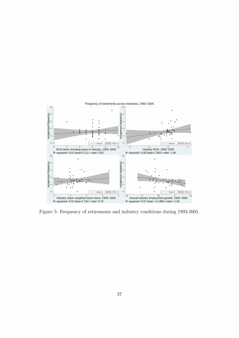
02

46

810

exog

enou

s fr

eque

ncy

0 2 4 6 8 10

ROA down−trending years in industry, 1993−2005

linear fit 95% CI

R−squared= 0.01 beta=0.111 t−stat= 0.83

02

46

810

exog

enou

s fr

eque

ncy

−.2 −.1 0 .1

Industry ROA, 1993−2005

linear fit 95% CI

R−squared= 0.05 beta=7.343 t−stat= 1.56

02

46

810

exog

enou

s fr

eque

ncy

0 .1 .2 .3 .4

Industry value−weighted stock return, 1993−2005

linear fit 95% CI

R−squared= 0.01 beta=2.734 t−stat= 0.70

02

46

810

exog

enou

s fr

eque

ncy

−.05 0 .05 .1 .15

Annual industry employment growth, 1993−2005

linear fit 95% CI

R−squared= 0.07 beta=−11.880 t−stat=−1.81

Frequency of retirements across industries, 1993−2005

Figure 5: Frequency of retirements and industry conditions during 1993-2005.

37

2.4

6.2

2.43.0

6.5

1.3

3.4

5.9

1.6

3.7

4.9

0.502

46

8P

erce

nt

1 2 3 4

by quartile of industry ROA

% Exogenous % Unclassified% Forced

3.0

4.8

1.0

3.2

6.0

1.9

3.2

6.5

1.1

3.3

6.7

2.30

24

68

Per

cent

1 2 3 4

by quartile of industry ROA down−trending years

% Exogenous % Unclassified% Forced

3.1

5.9

1.7

2.9

5.8

1.6

3.2

6.6

1.3

3.4

5.2

1.4

02

46

8P

erce

nt

1 2 3 4

by quartile of industry stock returns

% Exogenous % Unclassified% Forced

3.4

5.4

0.9

3.9

6.7

1.3

2.7

5.8

2.22.6

5.6

1.5

02

46

8P

erce

nt

1 2 3 4

by quartile of industry employment growth

% Exogenous % Unclassified% Forced

Frequency of turnover across industries

Figure 6: Frequency of turnover types as a function of industry conditions, 1993-2005.

38

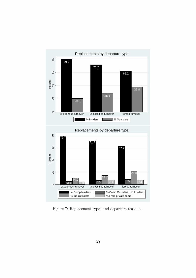
79.7

20.3

71.7

28.3

62.2

37.8

020

4060

80P

erce

nt

exogenous turnover unclassified turnover forced turnover

Replacements by departure type

% Insiders % Outsiders

79.7

4.910.9

4.5

71.7

6.5

14.7

7.1

62.2

8.5

21.8

7.5

020

4060

80P

erce

nt

exogenous turnover unclassified turnover forced turnover

Replacements by departure type

% Comp Insiders % Comp Outsiders, Ind Insiders% Ind Outsiders % From private comp

Figure 7: Replacement types and departure reasons.

39

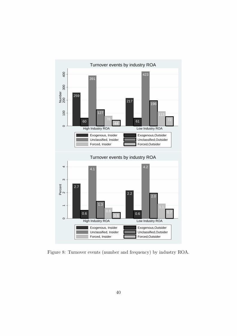
259

60

391

127

7844

217

61

423

196

113

72

010

020

030

040

0N

umbe

r

High Industry ROA Low Industry ROA

Turnover events by industry ROA

Exogenous, Insider Exogenous,Outsider Unclassified, Insider Unclassified,Outsider Forced, Insider Forced,Outsider

2.7

0.6

4.1

1.3

0.80.5

2.2

0.6

4.2

2.0

1.1

0.7

01

23

4P

erce

nt

High Industry ROA Low Industry ROA

Turnover events by industry ROA

Exogenous, Insider Exogenous,Outsider Unclassified, Insider Unclassified,Outsider Forced, Insider Forced,Outsider

Figure 8: Turnover events (number and frequency) by industry ROA.

40

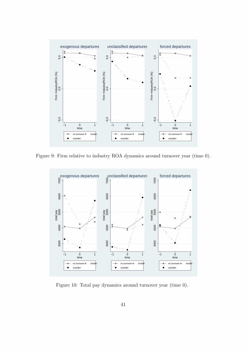
−5.

00.

05.

0F

irm−

Indu

stry

RO

A (

%)

−1 0 1time

no turnover insider

outsider

exogenous departures

−5.

00.

05.

0F

irm−

Indu

stry

RO

A (

%)

−1 0 1time

no turnover insider

outsider

unclassified departures

−5.

00.

05.

0F

irm−

Indu

stry

RO

A (

%)

−1 0 1time

no turnover insider

outsider

forced departures

Figure 9: Firm relative to industry ROA dynamics around turnover year (time 0).

3000

4000

5000

6000

7000

tota

l pay

−1 0 1time

no turnover insider

outsider

exogenous departures

3000

4000

5000

6000

7000

tota

l pay

−1 0 1time

no turnover insider

outsider

unclassified departures

3000

4000

5000

6000

7000

tota

l pay

−1 0 1time

no turnover insider

outsider

forced departures

Figure 10: Total pay dynamics around turnover year (time 0).

41

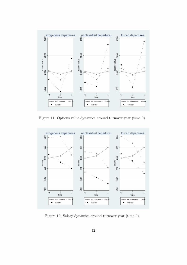
1000

2000

3000

4000

optio

ns v

alue

−1 0 1time

no turnover insider

outsider

exogenous departures

1000

2000

3000

4000

optio

ns v

alue

−1 0 1time

no turnover insider

outsider

unclassified departures

1000

2000

3000

4000

optio

ns v

alue

−1 0 1time

no turnover insider

outsider

forced departures

Figure 11: Options value dynamics around turnover year (time 0).

450

500

550

600

650

700

sala

ry

−1 0 1time

no turnover insider

outsider

exogenous departures

450

500

550

600

650

700

sala

ry

−1 0 1time

no turnover insider

outsider

unclassified departures

450

500

550

600

650

700

sala

ry

−1 0 1time

no turnover insider

outsider

forced departures

Figure 12: Salary dynamics around turnover year (time 0).

42

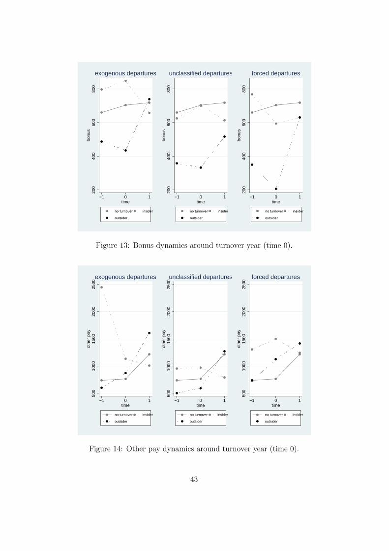
200

400

600

800

bonu

s

−1 0 1time

no turnover insider

outsider

exogenous departures

200

400

600

800

bonu

s

−1 0 1time

no turnover insider

outsider

unclassified departures

200

400

600

800

bonu

s

−1 0 1time

no turnover insider

outsider

forced departures

Figure 13: Bonus dynamics around turnover year (time 0).

500

1000

1500

2000

2500

othe

r pa

y

−1 0 1time

no turnover insider

outsider

exogenous departures

500

1000

1500

2000

2500

othe

r pa

y

−1 0 1time

no turnover insider

outsider

unclassified departures

500

1000

1500

2000

2500

othe

r pa

y

−1 0 1time

no turnover insider

outsider

forced departures

Figure 14: Other pay dynamics around turnover year (time 0).

43

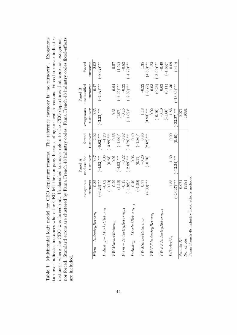
Tab

le1:

Mult

inom

ial

logi

tm

odel

for

CE

Odep

artu

rere

ason

s.T

he

refe

rence

cate

gory

is“n

otu

rnov

er”.

Exog

enou

stu

rnov

erin

dic

ates

inst

ance

sw

her

eth

eC

EO

left

the

com

pan

ybec

ause

ofag

eor

hea

lth

reas

ons.

For

ced

turn

over

indic

ates

inst

ance

sw

her

eth

eC

EO

was

forc

edou

t.U

ncl

assi

fied

turn

over

refe

rsto

the

CE

Odep

artu

res

that

wer

enot

exog

enou

s,nor

forc

ed.

Sta

ndar

der

rors

are

clust

ered

by

Fam

aFre

nch

48in

dust

ryco

des

.Fam

aFre

nch

48in

dust

ryco

des

fixed

-effec

tsar

ein

cluded

.

Pan

elA

Pan

elB

exog

enou

sun

clas

sifie

dfo

rced

exog

enou

sun

clas

sifie

dfo

rced

turn

over

turn

over

turn

over

turn

over

turn

over

turn

over

Fir

m−

Indust

ryR

eturn

t–0

.35

–0.4

7–2

.02

–0.3

5–0

.47

–2.0

2(–

3.23

)∗∗∗

(–4.

92)∗∗∗

(–8.

62)∗∗∗

(–3.

23)∗∗∗

(–4.

92)∗∗∗

(–8.

62)∗∗∗

Indust

ry−

Mark

etR

eturn

t–0

.02

0.03

–1.2

3(–

0.10

)(0

.23)

(–3.

99)∗∗∗

VW

Mark

etR

eturn

t0.

29–0

.91

–0.6

60.

31–0

.94

0.57

(1.1

6)(–

4.02

)∗∗∗

(–1.

66)∗

(1.0

7)(–

3.65

)∗∗∗

(1.5

2)F

irm−

Indust

ryR

eturn

t−1

–0.1

5–0

.22

–0.8

2–0

.15

–0.2

2–0

.82

(–1.

82)∗

(–2.

89)∗∗∗

(–4.

79)∗∗∗

(–1.

82)∗

(–2.

89)∗∗∗

(–4.

79)∗∗∗

Indust

ry−

Mark

etR

eturn

t−1

–0.4

00.

03–0

.49

(–1.

60)

(0.1

1)(–

1.86

)∗

VW

Mark

etR

eturn

t−1

0.77

–0.2

00.

861.

18–0

.22

1.35

(4.0

0)∗∗∗

(–0.

76)

(2.6

2)∗∗∗

(3.9

3)∗∗∗

(–0.

72)

(4.5

0)∗∗∗

VW

FF

Indust

ryR

eturn

t–0

.02

0.03

–1.2

3(–

0.10

)(0

.23)

(–3.

99)∗∗∗

VW

FF

Indust

ryR

eturn

t−1

–0.4

00.

03–0

.49

(–1.

60)

(0.1

1)(–

1.86

)∗

IsU

nder

65t

–1.8

5–1

.30

0.09

–1.8

5–1

.30

0.09

(–23

.27)∗∗∗

(–13

.34)∗∗∗

(0.4

0)(–

23.2

7)∗∗∗

(–13

.34)∗∗∗

(0.4

0)P

seud

oR

20.

071

0.07

1N

o.of

obs

1938

119

381

Fam

aFr

ench

48in

dust

ryfix

edeff

ects

incl

uded

44

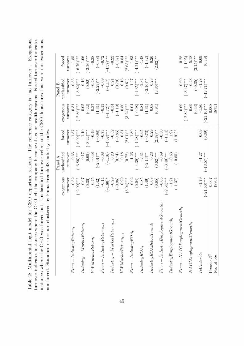
Tab

le2:

Mult

inom

ial

logi

tm

odel

for

CE

Odep

artu

rere

ason

s.T

he

refe

rence

cate

gory

is“n

otu

rnov

er”.

Exog

enou

stu

rnov

erin

dic

ates

inst

ance

sw

her

eth

eC

EO

left

the

com

pan

ybec

ause

ofag

eor

hea

lth

reas

ons.

For

ced

turn

over

indic

ates

inst

ance

sw

her

eth

eC

EO

was

forc

edou

t.U

ncl

assi

fied

turn

over

refe

rsto

the

CE

Odep

artu

res

that

wer

enot

exog

enou

s,nor

forc

ed.

Sta

ndar

der

rors

are

clust

ered

by

Fam

aFre

nch

48in

dust

ryco

des

.

Pan

elA

Pan

elB

exog

enou

sun

clas

sifie

dfo

rced

exog

enou

sun

clas

sifie

dfo

rced

turn

over

turn

over

turn

over

turn

over

turn

over

turn

over

Fir

m−

Indust

ryR

eturn

t–0

.32

–0.3

5–1

.87

–0.3

1–0

.35

–1.8

5(–

2.90

)∗∗∗

(–3.

86)∗∗∗

(–6.

90)∗∗∗

(–2.

86)∗∗∗

(–3.

82)∗∗∗

(–6.

76)∗∗∗

Indust

ry−

Mark

etR

eturn

t0.

070.

17–1

.10

0.05

0.16

–1.0

6(0

.30)

(0.9

5)(–

3.22

)∗∗∗

(0.2

2)(0

.92)

(–3.

26)∗∗∗

VW

Mark

etR

eturn

t0.

45–0

.48

–0.4

90.

37–0

.48

–0.3

8(1

.42)

(–2.

01)∗∗

(–0.

98)

(1.3

1)(–

2.29

)∗∗

(–0.

88)

Fir

m−

Indust

ryR

eturn

t−1

–0.1

4–0

.08

–0.7

3–0

.13

–0.0

9–0

.72

(–1.

80)∗

(–1.

16)

(–4.

62)∗∗∗

(–1.

72)∗

(–1.

17)

(–4.

57)∗∗∗

Indust

ry−

Mark

etR

eturn

t−1

–0.2

90.

20–0

.32

–0.3

40.

21–0

.22

(–0.

96)

(0.7

4)(–

0.85

)(–

1.19

)(0

.79)

(–0.

67)

VW

Mark

etR

eturn

t−1

0.99

0.18

0.81

0.80

0.16

0.84

(3.9

4)∗∗∗

(0.7

2)(2

.01)∗∗

(3.2

4)∗∗∗

(0.6

1)(2

.65)∗∗∗

Fir

m−

Indust

ryR

OA

t0.

02–1

.26

–1.8

9–0

.04

–1.2

7–1

.93

(0.0

4)(–

4.39

)∗∗∗

(–4.

28)∗∗∗

(–0.

08)

(–4.

35)∗∗∗

(–4.

21)∗∗∗

Indust

ryR

OA

t0.

85–2

.31

–0.9

50.

84–2

.34

–1.4

8(1

.49)

(–2.

16)∗∗

(–0.

73)

(1.3

1)(–

2.10

)∗∗

(–1.

32)

Indust

ryR

OA

Bel

owT

rend

t0.

080.

230.

290.

080.

230.

26(0

.85)

(3.6

2)∗∗∗

(2.1

8)∗∗

(0.9

4)(3

.85)∗∗∗

(2.0

2)∗∗

Fir

m−

Indust

ryE

mplo

ym

entG

row

tht

–0.6

5–0

.69

–0.3

0(–

2.64

)∗∗∗

(–3.

40)∗∗∗

(–1.

14)

Indust

ryE

mplo

ym

entG

row

tht

–1.2

1–0

.63

1.97

(–1.

37)

(–0.

85)

(1.9

1)∗

Fir

m−

NA

IC

Em

plo

ym

entG

row

tht

–0.6

9–0

.69

–0.2

8(–

2.82

)∗∗∗

(–3.

47)∗∗∗

(–1.

05)

NA

IC

Em

plo

ym

entG

row

tht

0.69

–0.4

35.

18(0

.43)

(–0.

35)

(3.1

5)∗∗∗

IsU

nder

65t

–1.7

9–1

.27

0.09

–1.8

0–1

.28

0.09

(–21

.50)∗∗∗

(–13

.57)∗∗∗

(0.3

9)(–

21.1

0)∗∗∗

(–13

.71)∗∗∗

(0.3

9)P

seud

oR

20.

067

0.06

8N

o.of

obs

1880

418

751

45

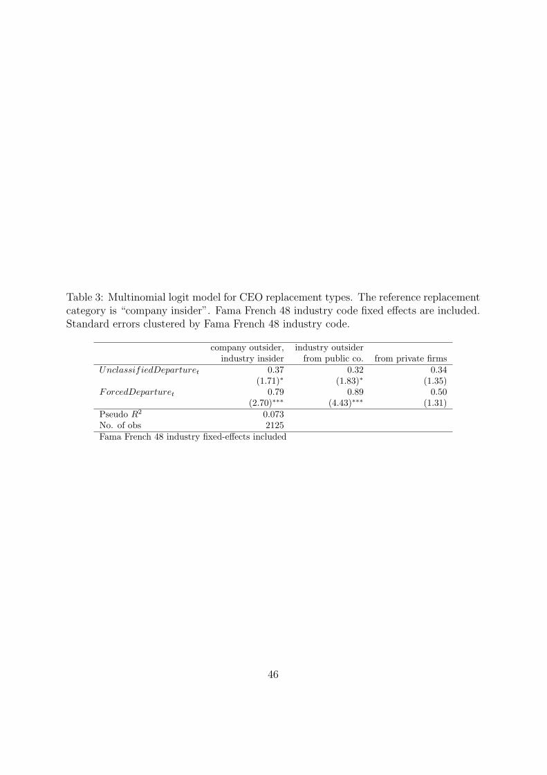
Table 3: Multinomial logit model for CEO replacement types. The reference replacementcategory is “company insider”. Fama French 48 industry code fixed effects are included.Standard errors clustered by Fama French 48 industry code.

company outsider, industry outsiderindustry insider from public co. from private firms

UnclassifiedDeparturet 0.37 0.32 0.34(1.71)∗ (1.83)∗ (1.35)

ForcedDeparturet 0.79 0.89 0.50(2.70)∗∗∗ (4.43)∗∗∗ (1.31)

Pseudo R2 0.073No. of obs 2125Fama French 48 industry fixed-effects included

46

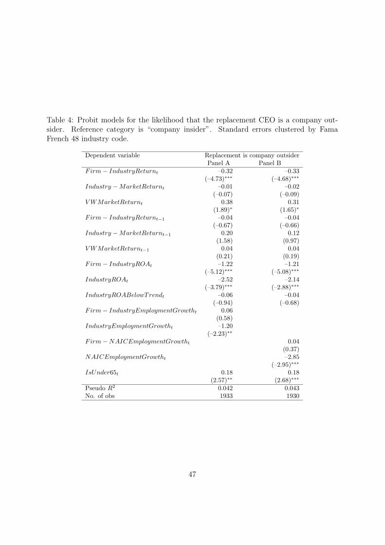
Table 4: Probit models for the likelihood that the replacement CEO is a company out-sider. Reference category is “company insider”. Standard errors clustered by FamaFrench 48 industry code.

Dependent variable Replacement is company outsiderPanel A Panel B

Firm− IndustryReturnt –0.32 –0.33(–4.73)∗∗∗ (–4.68)∗∗∗

Industry −MarketReturnt –0.01 –0.02(–0.07) (–0.09)

V WMarketReturnt 0.38 0.31(1.89)∗ (1.65)∗

Firm− IndustryReturnt−1 –0.04 –0.04(–0.67) (–0.66)

Industry −MarketReturnt−1 0.20 0.12(1.58) (0.97)

V WMarketReturnt−1 0.04 0.04(0.21) (0.19)

Firm− IndustryROAt –1.22 –1.21(–5.12)∗∗∗ (–5.08)∗∗∗

IndustryROAt –2.52 –2.14(–3.79)∗∗∗ (–2.88)∗∗∗

IndustryROABelowTrendt –0.06 –0.04(–0.94) (–0.68)

Firm− IndustryEmploymentGrowtht 0.06(0.58)

IndustryEmploymentGrowtht –1.20(–2.23)∗∗

Firm−NAICEmploymentGrowtht 0.04(0.37)

NAICEmploymentGrowtht –2.85(–2.95)∗∗∗

IsUnder65t 0.18 0.18(2.57)∗∗ (2.68)∗∗∗

Pseudo R2 0.042 0.043No. of obs 1933 1930

47

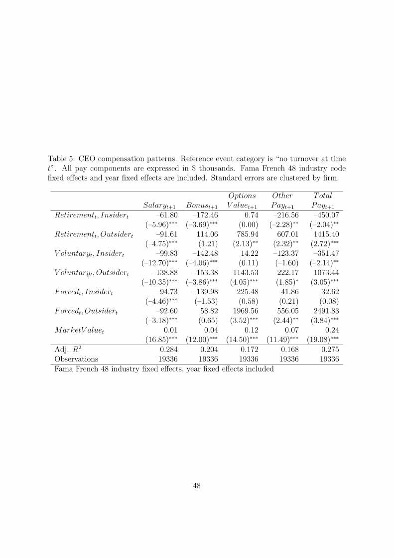
Table 5: CEO compensation patterns. Reference event category is “no turnover at timet”. All pay components are expressed in $ thousands. Fama French 48 industry codefixed effects and year fixed effects are included. Standard errors are clustered by firm.

Options Other TotalSalaryt+1 Bonust+1 V aluet+1 Payt+1 Payt+1

Retirementt, Insidert –61.80 –172.46 0.74 –216.56 –450.07(–5.96)∗∗∗ (–3.69)∗∗∗ (0.00) (–2.28)∗∗ (–2.04)∗∗

Retirementt, Outsidert –91.61 114.06 785.94 607.01 1415.40(–4.75)∗∗∗ (1.21) (2.13)∗∗ (2.32)∗∗ (2.72)∗∗∗

V oluntaryt, Insidert –99.83 –142.48 14.22 –123.37 –351.47(–12.70)∗∗∗ (–4.06)∗∗∗ (0.11) (–1.60) (–2.14)∗∗

V oluntaryt, Outsidert –138.88 –153.38 1143.53 222.17 1073.44(–10.35)∗∗∗ (–3.86)∗∗∗ (4.05)∗∗∗ (1.85)∗ (3.05)∗∗∗

Forcedt, Insidert –94.73 –139.98 225.48 41.86 32.62(–4.46)∗∗∗ (–1.53) (0.58) (0.21) (0.08)

Forcedt, Outsidert –92.60 58.82 1969.56 556.05 2491.83(–3.18)∗∗∗ (0.65) (3.52)∗∗∗ (2.44)∗∗ (3.84)∗∗∗

MarketV aluet 0.01 0.04 0.12 0.07 0.24(16.85)∗∗∗ (12.00)∗∗∗ (14.50)∗∗∗ (11.49)∗∗∗ (19.08)∗∗∗

Adj. R2 0.284 0.204 0.172 0.168 0.275Observations 19336 19336 19336 19336 19336Fama French 48 industry fixed effects, year fixed effects included

48