Centripetal Forces in China’s Economic Takeoff ... · Centripetal Forces in China’s Economic...

Centripetal Forces in China’s Economic Takeoff

ANURADHA DAYAL-GULATI and AASIM M. HUSAIN*

This paper uses provincial time series data from the People’s Republic of China toempirically investigate two propositions relating to economic development: (i) thateconomic takeoff—or an acceleration in economic growth—is associated withinflows of foreign direct investment (FDI), possibly through technological transfer;and (ii) that takeoff is accompanied, at least in the short term, by widening incomeinequality. The results indicate that FDI flows have increased the rate of conver-gence in per capita incomes across China’s provinces. However, the pattern of FDI,which has gone mainly to the relatively wealthy provinces, has caused differentprovinces to converge toward different steady states. [JEL O4, O11, O18]

Economic takeoff is often associated with technological transfer from othercountries, largely through foreign direct investment (FDI). Also, economic

development is often linked with rising inequality, at least in the short term. Thelogic tying these two ideas together is straightforward—relatively prosperouscountries or regions tend to receive more FDI because they have the existinginfrastructure to support such projects. Hence, inequality across countries orregions widens as a result of FDI, which in turn helps achieve economic takeoff.

364

IMF Staff PapersVol. 49, No. 3© 2002 International Monetary Fund

*Anuradha Dayal-Gulati is a Clinical Associate Professor at the Kellogg Graduate School ofManagement, Northwestern University, and Aasim M. Husain is Assistant to the Director in the ResearchDepartment of the International Monetary Fund. The majority of this work was completed when AnuradhaDayal-Gulati was an Economist in the IMF Institute and Aasim Husain was a Senior Economist in the Asiaand Pacific Department of the IMF. We would like to thank, without implicating, Jahangir Aziz, TamimBayoumi, Paul Cashin, Mohsin Khan, Peter Montiel, Ichiro Otani, David Robinson, Reza Vaez-Zadeh, andan anonymous referee for helpful comments on earlier drafts of this paper. We are also indebted to KirstenFitchett, Lakshmi Sahasranam, Bin Zhang, and Rui Zhao for their help with assembling the data.

Cross-country empirical analysis of these propositions, however, is compli-cated by institutional and policy differences across countries, which can rendercomparisons problematic. As such caveats do not apply across regions of the samecountry, provincial-level data from China over the past two decades can be used toprovide interesting empirical insight into these propositions relating to the processof economic development.1, 2

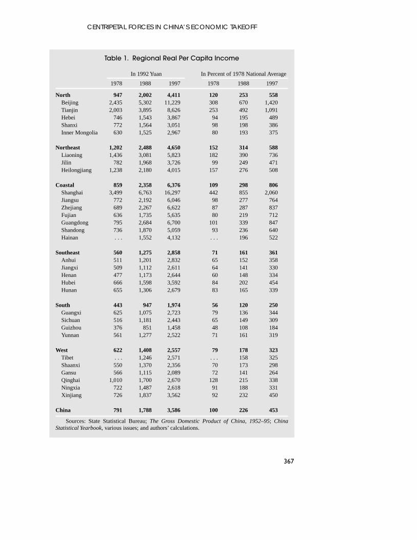
China’s growth performance since the initiation of market-oriented reform in1978 has been impressive. Real GDP has grown by an average annual rate ofalmost 10 percent; real per capita output has averaged 81/4 percent a year. Thiseconomic takeoff has coincided with large inflows of FDI, which have averagedover US$40 billion (51/2 percent of GDP) annually in recent years. At the sametime, however, the variation in economic performance across provinces haswidened, particularly since the late 1980s. After declining in the late 1970s and1980s, the dispersion of (the natural logarithm of) provincial per capita incomesincreased steadily in the 1990s (Figure 1).3 In 1978, real per capita income in therichest province was around six times that of the poorest; by 1997, the multiplehad risen to almost eight (Table 1). Similarly, the pattern of FDI across provincesand regions has differed sharply. The coastal region, for example, saw FDI inflowsaveraging over 9 percent of regional GDP during 1993–97, while FDI in thewestern and southeastern regions averaged only 1–2 percent over the same period.

The apparent widening disparity across China’s provinces—or groups ofprovinces—raises the question of whether provincial per capita incomes havediverged and, if so, why? This paper investigates the variation in economic perfor-mance across provinces and empirically examines whether the poorer provincesgrew faster than the richer ones, which would suggest that all the provinces wereconverging to the same steady-state real per capita income level.4 In addition, thepaper investigates the role of FDI and other structural and policy factors—including the share of investment in provincial GDP, the dominance of state-owned enterprises (SOEs) in industrial output, and the role of the bankingsystem—on economic growth over the period 1978–97.

The analysis presented in this paper indicates that absolute convergence—convergence of real per capita incomes in all provinces to the same steady-statelevel—does not appear to hold over the past two decades, although there appearsto be evidence of conditional convergence—that is, convergence of provincial percapita incomes to their own steady states. While structural characteristics of theprovincial economies—such as the share of investment to GDP and the share of

CENTRIPETAL FORCES IN CHINA’S ECONOMIC TAKEOFF

365

1All references to China in this paper are to the People’s Republic of China.2Strictly speaking, propositions in the literature regarding rising Kuznets-type income inequality

generally relate to widening disparity across income groups within a given country or region (see, forexample, Ben-David, 1993), while the analysis reported below refers to inequality of income growth ratesacross provinces or regions within China. Clearly, widening disparity of one type need not necessarily beassociated with greater inequality in the other sense.

3The coefficient of variation—the standard deviation divided by the mean—of real per capita incomes(also depicted in Figure 1) shows a similar pattern.

4As noted by Cashin and Sahay (1996), convergence of per capita incomes is a necessary, but notsufficient, condition for a reduction in the dispersion of per capita incomes.

SOEs in industrial output—have had some effect, the regional disparities appearto be influenced primarily by the relative importance of FDI to the region. Indeed,the inclusion of an FDI variable in the regressions results in a sizable increase inthe estimated rate of convergence of each region to its own steady state.

I. Absolute and Conditional Convergence

There is a growing literature on convergence of per capita incomes across and withincountries. If economies possess similar levels of technology and have similar prefer-ences, then the neoclassical growth model predicts that all provinces would convergeto similar levels of real per capita income in the steady state. This is known as abso-lute β convergence. Convergence of per capita incomes in this model is driven by theassumption of diminishing returns to capital. When the stock of capital is low, eachaddition to capital stock generates large increases in output. These increments tend todecrease as the stock of capital increases. Accordingly, if the only difference betweeneconomies is the initial level of capital stock, the neoclassical growth model predictsthat poorer economies will grow faster than rich ones. Regions with lower startingcapital-labor ratios will have higher per capita growth rates.

The empirical evidence suggests that convergence is absolute within homoge-neous groups of economies. Barro and Sala-i-Martin (1991, 1992a, 1992b)examine data for the U.S. states from 1880–1990, for Japanese prefectures over

Anuradha Dayal-Gulati and Aasim M. Husain

366

0.44

0.47

0.49

0.52

0.54

0.63

0.66

0.69

0.72

0.75

Coefficient of Variation(log levels; right scale)

Standard Deviation

(log levels; left scale)

1978 1981 1984 1987 1990 1993 1996

Figure 1. Provinces’ Real Per Capita Incomes, 1978–97


367

Table 1. Regional Real Per Capita Income

In 1992 Yuan In Percent of 1978 National Average

1978 1988 1997 1978 1988 1997

North 947 2,002 4,411 120 253 558Beijing 2,435 5,302 11,229 308 670 1,420Tianjin 2,003 3,895 8,626 253 492 1,091Hebei 746 1,543 3,867 94 195 489Shanxi 772 1,564 3,051 98 198 386Inner Mongolia 630 1,525 2,967 80 193 375

Northeast 1,202 2,488 4,650 152 314 588Liaoning 1,436 3,081 5,823 182 390 736Jilin 782 1,968 3,726 99 249 471Heilongjiang 1,238 2,180 4,015 157 276 508

Coastal 859 2,358 6,376 109 298 806Shanghai 3,499 6,763 16,297 442 855 2,060Jiangsu 772 2,192 6,046 98 277 764Zhejiang 689 2,267 6,622 87 287 837Fujian 636 1,735 5,635 80 219 712Guangdong 795 2,684 6,700 101 339 847Shandong 736 1,870 5,059 93 236 640Hainan . . . 1,552 4,132 . . . 196 522

Southeast 560 1,275 2,858 71 161 361Anhui 511 1,201 2,832 65 152 358Jiangxi 509 1,112 2,611 64 141 330Henan 477 1,173 2,644 60 148 334Hubei 666 1,598 3,592 84 202 454Hunan 655 1,306 2,679 83 165 339

South 443 947 1,974 56 120 250Guangxi 625 1,075 2,723 79 136 344Sichuan 516 1,181 2,443 65 149 309Guizhou 376 851 1,458 48 108 184Yunnan 561 1,277 2,522 71 161 319

West 622 1,408 2,557 79 178 323Tibet . . . 1,246 2,571 . . . 158 325Shaanxi 550 1,370 2,356 70 173 298Gansu 566 1,115 2,089 72 141 264Qinghai 1,010 1,700 2,670 128 215 338Ningxia 722 1,487 2,618 91 188 331Xinjiang 726 1,837 3,562 92 232 450

China 791 1,788 3,586 100 226 453

Sources: State Statistical Bureau; The Gross Domestic Product of China, 1952–95; ChinaStatistical Yearbook, various issues; and authors’ calculations.


368

the period 1930–90, and for the regions of eight European countries from1950–90. They find that convergence is absolute in that it applies when no othervariable other than the initial level of per capita income is held constant. Cashinand Sahay (1996) examine convergence within India and find that variations in thesteady state values across states are not significant, implying absoluteconvergence.

If economies vary in their saving rates and technologies, then the neoclassicalgrowth model predicts conditional β convergence—provincial per capita incomesstill converge, but this convergence is conditional on each economy’s own steadystate. Across countries, the accumulated empirical evidence suggests that conver-gence is conditional—after taking into account the effects of the rate of investmentand public policies on per capita growth.5 In most cases, the empirical work doesnot provide robust estimates for the effects of a specific government policy ongrowth, but it shows that the overall package of policies matters a great deal. Thetendency towards convergence is even stronger when a measure of human capitalin the form of educational attainment and health is included as an explanatoryvariable.6

Thus, if all the provinces of China have similar levels of technology andsimilar preferences, then they would converge to the same level of per capitaincome in the steady state (absolute convergence). If, on the other hand, provinces’technologies vary—possibly on account of their ability to attract FDI—they wouldnot be expected to converge to the same steady state, at least as long as their attrac-tiveness to FDI remained varied.7

Capital and labor mobility—or openness—affect the rate of convergence. Forexample, the availability of foreign finance makes it easier to acquire physicalcapital. With the associated increase in the capital stock, diminishing returns set infaster than they would in a closed economy. Hence, the speed of convergence isgreater in open economies than in closed ones.8

The evidence from China suggests that mobility of labor and capital acrossprovinces in China has been limited by policies.9 For instance, permission forhouseholds to move from rural to urban areas has been restricted, and capital

5Public policies include the volume of consumption spending and the associated level of taxation,some form of public investment, and institutional infrastructure.

6See Barro and Sala-i-Martin (1995) for a review of this literature. 7The creation of special economic zones in some of the coastal provinces may have facilitated the

inflow of FDI. To that extent, greater inflows of FDI could be associated with higher capital mobility,thereby raising the rate of convergence. Nevertheless, other factors, such as proximity to Hong Kong SARand Taiwan Province of China—where much of the FDI originated—and their relatively richer humancapital endowment were likely also important factors explaining the coastal provinces’ ability to attractFDI. Such differential ability to attract FDI, rather than access to FDI, would explain provinces’ conver-gences to different steady states, as suggested by our results.

8Labor mobility is analogous to capital mobility and also tends to speed up an economy’s convergencetowards its steady state position. While the empirical evidence for convergence in the regional data aftertaking into account net migration is not definitive, Cashin and Sahay (1996) find that migration is an espe-cially slow means of equalizing per capita incomes.

9Appendix II provides some background information on policies relating to capital and labormobility.

mobility has also been dampened through tax policies and state control over banklending. Therefore, with partial capital and labor mobility, output convergenceacross provinces is likely to be more gradual. However, policies have also soughtto directly redistribute incomes from relatively rich regions to poorer provinces,thereby boosting the rate of convergence. Thus, a relevant question for China iswhether policies have, in total, contributed to the equalization of provincial percapita incomes.

Previous empirical studies of provincial economic performance and conver-gence in China include Bell, Khor, and Kochhar (1993) and Zhao (1998). Bell,Khor, and Kochhar, using the real annual average provincial growth rate during1981–90, find that poorer provinces tended to grow faster than richer ones. Thisfinding appears to depend critically on the sample period, however, during muchof which there was a rapid expansion in agricultural output following the liberal-ization of the agricultural sector. Indeed, as Figure 1 indicates, the dispersion ofprovincial per capita incomes narrowed considerably during this period, beforeincreasing steadily in the 1990s. Bell, Khor, and Kochhar also find that the propor-tion of nonstate sector output in total output was positively related to growth,while there was not a statistically significant relationship in their growth regres-sion between FDI and growth.10 Zhao observes that the evolution of the ratio ofreal per capita GDP in the richest province to that in the poorest province was U-shaped, and empirically investigates the role of capital mobility in explaining thistrend. She finds that capital mobility across China’s provinces was relativelylimited during the 1980s and 1990s (see Appendix II).

Very recent work using our dataset by Graham and Wada (2001) and Aziz andDuenwald (2001) generally supports and extends our findings. Graham and Wadaempirically assess whether inflows of FDI may have been associated with anacceleration in total factor productivity (TFP) growth, possibly resulting fromtechnology transfer embodied in FDI inflows. They conclude that FDI has indeedcontributed to growth in the provinces and regions of China—particularly thecoastal region—that received sizable flows of this type, beyond what would beexpected from higher rates of capital formation enabled by the FDI. Aziz andDuenwald investigate the implications of alternative convergence tests on ourresults. Using the methodology suggested by Quah (1997) to more fully exploitinformation contained in the data, they compute kernel estimates of the relativeincome distribution of China’s provinces. Their results—that the distribution ofrelative incomes is clustering toward two separate relative income clubs, with thecoastal provinces (which received the most FDI) gravitating towards a higher percapita income mode than the other provinces—are consistent with our finding ofconditional convergence.

In another related recent study, Wei and Wu (2001) empirically assess the rela-tion between openness and rural-urban income inequality in Chinese cities andtheir adjacent rural areas during 1988–93. Defining openness as the ratio of


369

10By regressing average growth on only FDI, however, Bell, Khor, and Kochhar (1993) obtain asignificant positive coefficient.

exports to GDP, and allowing for endogeneity by using distance to major seaportsas an instrument for openness, they find that while average openness increased andoverall rural-urban inequality also went up during this period, the correlationacross cities was negative. Together with our results, this would seem to suggestthat within-province inequality has improved while interprovincial inequality hasworsened. However, such an interpretation is subject to at least two qualifications.First, the Wei and Wu results are based on a much shorter time period. Indeed, asillustrated in Figure 1, much of the rise in the dispersion of average per capitaincomes across provinces took place after the period studied by Wei and Wu.Second, special economic zones, which received a large share of China’s total FDIinflows, were excluded from Wei and Wu’s sample. The direction in which thisexclusion might affect their result is not clear.

II. Regional Economic Performance

The basic estimation sample covers 28 provinces and municipalities over theperiod 1978 to 1997.11 The output data used are provincial GDP in constant (1992yuan) prices based on provincial price deflators.12 These estimates are divided bythe provincial population estimates to get provincial real GDP per capita, which isused as a proxy for real per capita income.13 For analytical purposes, the data arealso divided into nonoverlapping intervals of five years each—1978–82, 1983–87,1988–92, and 1993–97. Using the rate of growth of per capita output over a five-year interval rather than a single year provides a simple means of smoothing outshort-run cyclical fluctuations in the rate of capacity utilization. This helps ensurethat this variable approximates output growth at the average rate of capacityutilization.14 Averages of the explanatory variables over the five-year intervals areused in the estimation procedures.

It is convenient for analytical purposes to divide the provinces and munic-ipalities of China into six geographic regions—northern, northeastern, coastal,southeastern, southern, and western. The northern region consists of Hebei,Shanxi, and Inner Mongolia, as well as the municipalities of Beijing andTianjin. The northeast, which comprises Liaoning, Jilin, and Heilongjiangprovinces, has a higher concentration of state-owned industry than the rest ofthe country. The coastal region—consisting of the municipality of Shanghai


370

11Hainan and Tibet Autonomous Region were excluded from the estimations owing to lack of datacovering the entire sample period. Data for Chongqing, which became an independent municipality in1997, are included in the data for Sichuan.

12See Appendix I for a description of the variables and data sources. 13Time series income data at a macro level are not available. Consequently, per capita incomes and

per capita output are used interchangeably in this paper.14Although there is some degree of arbitrariness in assuming that the duration of the business cycle

is five years and is synchronized across provinces and the periods chosen, a study by Khan and Kumar(1997) using a similar approach does not find that the results are sensitive to the choice of a three- or five-year average. It may also be noted that Husain (1998) finds that cycles were about that long in each regionin China, although the cycles tended not to be perfectly synchronized across regions.


371

and the provinces of Jiangsu, Zhejiang, Fujian, Shandong, Guangdong, andHainan—has been the recipient of the bulk of foreign direct investment (FDI),particularly from Hong Kong SAR. The southeastern provinces—Anhui,Jiangxi, Henan, Hubei, and Hunan—are adjacent to the coastal region and havereceived an increasing share of FDI in recent years. The southern region, whichincludes Guangxi, Sichuan, Guizhou, and Yunnan, is more dependent on theagricultural sector than the other regions. Finally, the western region,comprising Tibet Autonomous Region, Shaanxi, Gansu, Qinghai, Ningxia, andXinjiang, accounts for around one half of China’s land area but only 7 percentof its population.15

Growth Performance

Economic performance, as measured by the growth in real GDP per capita, hasvaried significantly across regions and over time (Table 2). For China as a whole,real per capita GDP growth averaged 6 percent in the early post-reform period(1978–82), but picked up markedly in 1983–87 following the introduction ofmarket-oriented reforms in the agricultural sector. Per capita income growthslowed during 1988–92, but picked up again in 1993–97 after the launch of amajor investment drive in the coastal region.

While the coastal region grew at a faster pace than the rest of the country ineach of the four subperiods, the relative performance of the other regions varied.For example, growth in the southeastern region exceeded the national average onlyin the first and last subperiods, while that in the northern and northeastern regionsexceeded the national average only in the last subperiod. As a result, the relativeposition of the regions in terms of the average level of real per capita GDP hasshifted, and each region’s share in China’s overall GDP has changed (Table 3). Theshare of the coastal region, for example, has risen from around one third in the late1970s to over 40 percent in recent years.

The data also indicate a strong positive relation between initial income and thepickup in growth during the post-reform period. As illustrated in Figure 2, theincrease in average growth between 1978–82 and 1993–97 was smallest for theinitially poorest southern region, and greatest for the initially richest northeasternand northern regions.

15While lumping municipalities and provinces is potentially problematic, we chose to maximize thesize of the sample by including municipalities for a number of reasons. First, municipalities are indepen-dent administrative units, in the same way as provinces, and data for both are collected and compiled inthe same fashion. Second, special features of municipalities—such as their relative prosperity and highdegree of urbanization—should be captured by variables included in the estimations reported below, suchas initial per capita income and agriculture’s share of output. Indeed, the municipalities did not stand outas outliers in the regressions, and when provincial dummies were included, coefficient estimates fordummies associated with municipalities were not out of line with those for provinces. Third, the disper-sion of provincial per capita incomes exhibits an even stronger increase in the 1990s when municipalitiesare excluded, suggesting that the convergence to different steady states finding does not rest on the inclu-sion of municipalities in our sample.


372

Table 2. Regional Per Capita Income Growth Rates(annual average; in percent)

1978–82 1983–87 1988–92 1993–97 1978–97

North 5.2 9.6 6.7 11.7 8.4Beijing 4.6 10.4 7.3 10.5 8.4Tianjin 5.3 8.7 4.7 12.9 8.0Hebei 4.1 9.5 8.1 13.6 9.0Shanxi 5.6 8.9 5.5 9.6 7.5Inner Mongolia 8.4 10.1 6.3 9.3 8.5

Northeast 3.9 10.2 5.6 9.3 7.4Liaoning 2.9 12.0 5.4 9.5 7.6Jilin 5.1 12.5 5.6 10.7 8.6Heilongjiang 4.5 6.6 5.7 8.4 6.4

Coastal 8.4 11.3 9.7 14.4 11.1Shanghai 5.3 7.6 6.8 13.5 8.4Jiangsu 8.2 12.8 9.9 14.3 11.4Zhejiang 11.9 13.8 9.1 15.7 12.6Fujian 10.4 10.3 10.7 17.0 12.2Guangdong 9.0 12.2 12.4 13.4 11.9Shandong 7.8 11.2 8.7 14.6 10.7Hainan1 . . . 6.6 13.7 8.7 10.4

Southeast 7.4 10.0 5.6 12.7 9.0Anhui 7.9 10.8 3.6 15.4 9.4Jiangxi 7.2 8.6 7.8 12.1 9.0Henan 7.3 11.5 5.9 12.7 9.4Hubei 8.8 10.1 5.7 12.6 9.3Hunan 5.9 8.3 5.6 10.7 7.7

South 6.7 9.1 6.6 10.3 8.3Guangxi 6.5 5.5 7.2 12.8 8.1Sichuan 6.6 10.6 6.4 10.3 8.5Guizhou 7.5 9.9 5.2 7.1 7.4Yunnan 7.0 8.8 7.7 9.2 8.2

West 4.8 10.7 6.7 8.2 7.7Tibet2 . . . –1.3 4.0 11.6 5.6Shaanxi 5.9 10.6 6.7 8.2 8.0Gansu 1.2 10.9 6.8 8.6 7.1Qinghai 2.5 7.7 3.2 7.2 5.3Ningxia 3.6 10.3 4.8 8.8 7.0Xinjiang 7.6 11.9 7.8 7.5 8.7

China 6.0 10.3 7.0 9.4 8.3


1Data cover 1985–97.2Data cover 1984–97.


373

Table 3. Regional Economic Indicators, 1978–97

Share of RegionalShare of Regional GDP Population in Totalin Total GDP (Percent) Population (Percent)

1978–80 1995–97 1978–80 1995–97

North 14.9 12.4 11.5 11.5Beijing 3.1 2.4 0.9 0.9Tianjin 2.4 1.6 0.8 0.7Hebei 5.2 5.1 5.3 5.4Shanxi 2.6 1.9 2.5 2.6Inner Mongolia 1.6 1.4 1.9 1.9

Northeast 13.7 10.1 9.1 8.6Liaoning 6.4 4.6 3.6 3.4Jilin 2.3 1.9 2.3 2.2Heilongjiang 5.0 3.5 3.3 3.1

Coastal 32.7 41.7 26.6 26.9Shanghai 7.4 4.3 1.2 1.1Jiangsu 7.4 8.8 6.1 5.9Zhejiang 3.9 6.1 3.9 3.6Fujian 1.9 3.8 2.6 2.7Guangdong 5.4 9.5 5.3 5.7Shandong 6.6 8.7 7.5 7.3Hainan1 . . . 0.6 . . . 0.6

Southeast 19.8 19.1 26.0 26.1Anhui 3.3 3.5 5.0 5.0Jiangxi 2.6 2.2 3.3 3.4Henan 5.0 5.3 7.4 7.6Hubei 4.6 4.3 4.8 4.8Hunan 4.4 3.9 5.4 5.3

South 12.8 12.0 19.8 19.3Guangxi 2.2 2.7 3.6 3.8Sichuan 7.3 6.1 10.2 9.3Guizhou 1.4 1.1 2.8 2.9Yunnan 2.0 2.1 3.2 3.3

West 6.0 4.8 7.0 7.5Tibet2 . . . 0.1 . . . 0.2Shaanxi 2.3 1.7 2.9 3.0Gansu 1.8 1.0 2.0 2.0Qinghai 0.4 0.3 0.4 0.4Ningxia 0.4 0.3 0.4 0.4Xinjiang 1.2 1.4 1.3 1.5

China 100.0 100.0 100.0 100.0



Economic Structure

A marked transformation in China’s economic structure has taken place since thelate 1970s. The share of the agricultural sector in GDP has fallen by some 10percentage points to 20 percent. At the same time, the ratio of total investment toGDP has risen steadily, accompanied by an expansion in investment spending bothby state enterprises as well as the nonstate sector.

While the structural transformation at the national level was generallyreflected in developments in each of the regions, there was significant variation inthe timing, pattern, and extent of transformation across regions. For example,reform of the agricultural sector was initially introduced in Anhui province in1978, and later adopted in almost all rural farm households by 1984.16

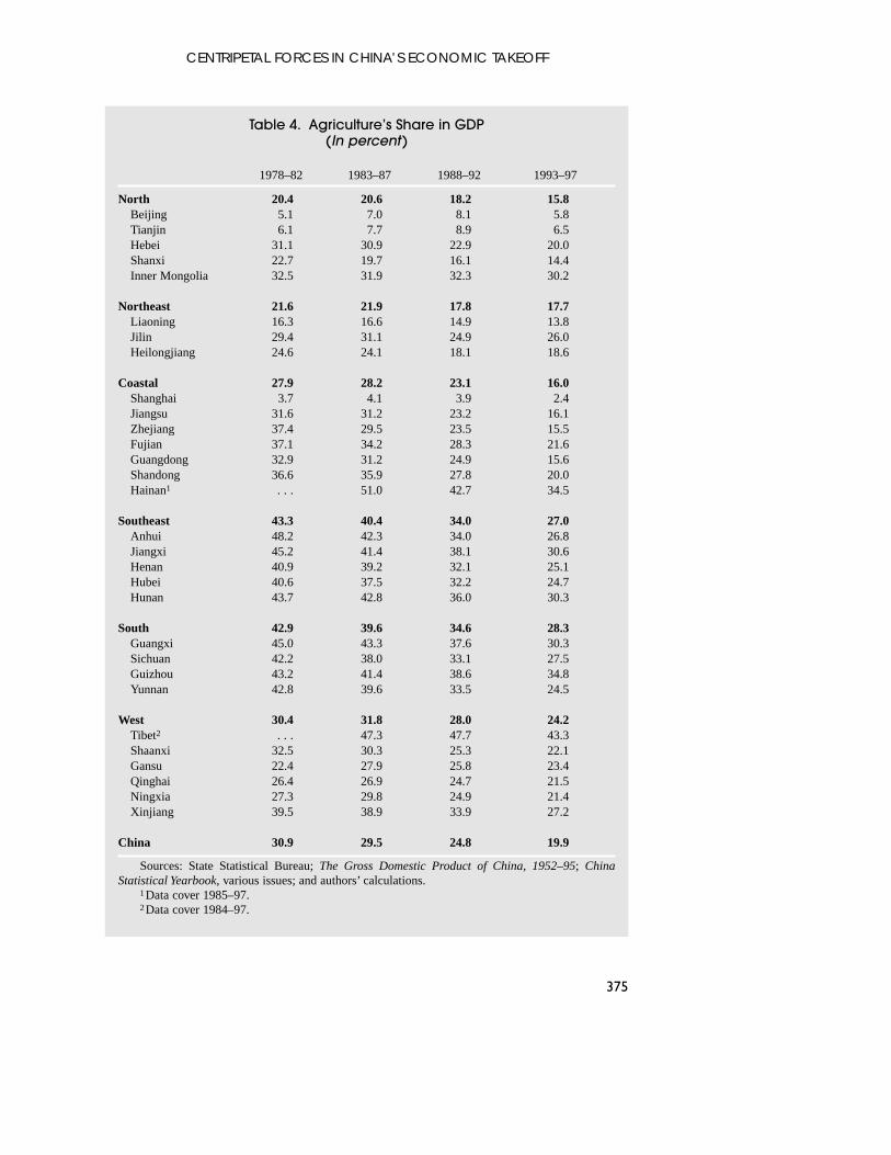
Consequently, the regions with the largest agricultural sectors (southern and south-eastern) at the start of the reform process experienced the steepest declines in agri-culture’s share in regional GDP (Table 4). By contrast, regions where theagricultural sector was relatively small at the outset (northern and northeastern)witnessed a much smaller decline in its share in regional GDP.

Regional differences in the pattern of investment were even more pronounced.The share of total investment in GDP increased sharply in the northern and coastal


374

16See Qian (1999).

0 20 40 60 80 100 120 140 1600

1.0

2.0

3.0

4.0

5.0

6.0

Southeast

West

SouthChina

Coastal

NorthNortheast

Incr

ease

in R

eal P

er C

apita

Inc

ome

Gro

wth

Bet

wee

n 19

78–8

2 an

d 19

93–9

7 (P

erce

ntag

e po

ints

)

Real Per Capita Income in 1978 (Percent of national average)

Figure 2. Regions’ Initial Income and Per Capita Growth Increases


375

Table 4. Agriculture’s Share in GDP (In percent)

1978–82 1983–87 1988–92 1993–97



Coastal 27.9 28.2 23.1 16.0Shanghai 3.7 4.1 3.9 2.4Jiangsu 31.6 31.2 23.2 16.1Zhejiang 37.4 29.5 23.5 15.5Fujian 37.1 34.2 28.3 21.6Guangdong 32.9 31.2 24.9 15.6Shandong 36.6 35.9 27.8 20.0Hainan1 . . . 51.0 42.7 34.5



West 30.4 31.8 28.0 24.2Tibet2 . . . 47.3 47.7 43.3Shaanxi 32.5 30.3 25.3 22.1Gansu 22.4 27.9 25.8 23.4Qinghai 26.4 26.9 24.7 21.5Ningxia 27.3 29.8 24.9 21.4Xinjiang 39.5 38.9 33.9 27.2

China 30.9 29.5 24.8 19.9




376

regions over the period as a whole but less so in the other areas. The westernregion had the highest share of investment in total output at the start of the sampleperiod (40 percent of GDP), which rose to 50 percent (Table 5). Despite the rela-tively high investment ratio, however, the large share of output produced by state-owned enterprises (SOEs)—about 75 percent—and constraints in their reformmay have led to a buildup of inventories. In the northern and northeastern regions,much of the rise in the investment rate was also on account of SOEs, while theincrease in the coastal region was mainly due to the nonstate sector.

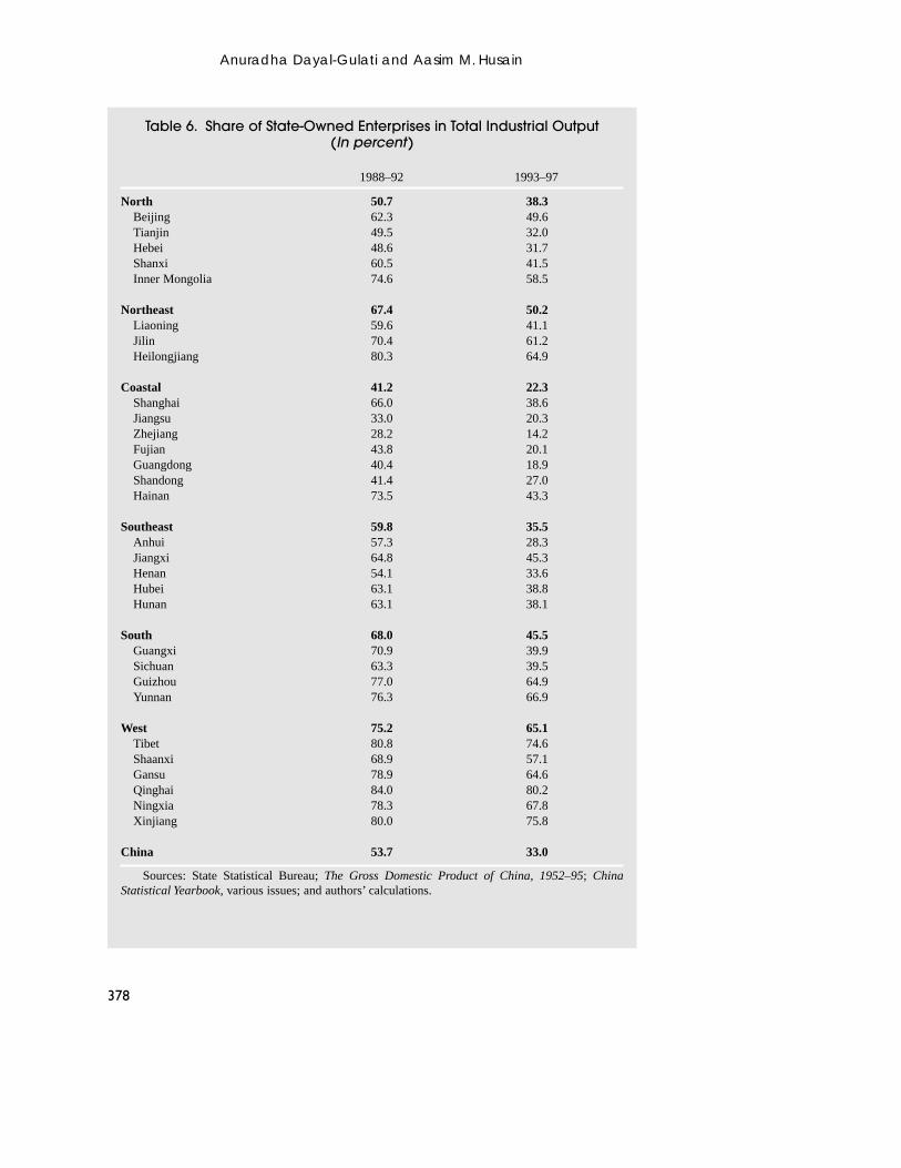
The preponderance of SOEs in provincial economies has varied across regionsas well. Although data on the share of state enterprises in total industrial output areavailable only from the late 1980s (Table 6), these indicate a sharp decline in theimportance of the state sector in the coastal and southeastern regions. By contrast,SOEs have continued to account for the majority of industrial output in the north-eastern and western regions.

Policies Affecting Economic Performance

Despite restrictions on internal capital mobility, policies have been geared towardattracting capital and technology from abroad. There was a marked shift inChina’s foreign investment policies in the second half of the 1980s, including theintroduction of special tax incentives to encourage investment in certain indus-tries. FDI flows increased sharply from less than US$1 billion in 1983 to overUS$40 billion in 1997. The inflows showed a dramatic increase in the coastalregion, where they rose to over 9 percent of provincial GDP and accounted for animportant source of investment spending (Table 7). More recently, the northernand northeastern regions have also seen a sizable increase in FDI inflows. Asillustrated in Figure 3, initially rich provinces have tended to attract relativelygreater inflows of FDI.

An important mechanism for reallocating financial capital across provinceshas been the pattern of lending by the banking system, which until the mid-1990swas subject to credit quotas set by the State Planning Commission (SPC) inconjunction with the People’s Bank of China (PBC). Credit quotas for eachprovince were established on an annual basis to meet policy objectives. Banks inprovinces with quotas that were high in relation to their deposit growth financedtheir lending by borrowing from the PBC, while banks in provinces where creditquotas were relatively tight ended up having to maintain high excess reserves withthe PBC. As a result, there was a close link between the credit plan and centralbank lending, and the PBC played an important role in redistributing financialresources across provinces.

These flows of financial capital appear to have reflected redistributive policyobjectives rather than consumption-smoothing or differences in rates of return oninvestment across provinces. Using data covering 1988–93, Lardy (1998) findsthat the provincial share of industrial output produced by SOEs was the mostimportant variable explaining variations in provincial loan to deposit ratios, with


377

Table 5. Ratio of Total Investment to GDP (In percent)

1978–82 1983–87 1988–92 1993–97



Coastal 27.9 35.7 40.0 47.9Shanghai 20.9 35.5 45.3 59.3Jiangsu 30.4 40.6 43.7 48.5Zhejiang 25.9 33.1 34.5 47.9Fujian 30.3 31.9 31.1 44.5Guangdong 29.2 34.9 36.6 43.6Shandong 32.0 36.1 43.5 46.8Hainan1 . . . . . . 61.2 57.7



West 40.4 43.1 45.8 50.6Tibet2 . . . . . . 45.9 47.1Shaanxi 34.5 42.7 43.2 46.7Gansu 37.9 37.7 41.6 40.2Qinghai 57.5 54.1 45.0 48.7Ningxia 54.0 58.1 57.8 51.8Xinjiang 44.9 47.4 53.8 63.5

China 35.1 36.0 35.7 40.6




378

Table 6. Share of State-Owned Enterprises in Total Industrial Output (In percent)

1988–92 1993–97

North 50.7 38.3Beijing 62.3 49.6Tianjin 49.5 32.0Hebei 48.6 31.7Shanxi 60.5 41.5Inner Mongolia 74.6 58.5

Northeast 67.4 50.2Liaoning 59.6 41.1Jilin 70.4 61.2Heilongjiang 80.3 64.9

Coastal 41.2 22.3Shanghai 66.0 38.6Jiangsu 33.0 20.3Zhejiang 28.2 14.2Fujian 43.8 20.1Guangdong 40.4 18.9Shandong 41.4 27.0Hainan 73.5 43.3

Southeast 59.8 35.5Anhui 57.3 28.3Jiangxi 64.8 45.3Henan 54.1 33.6Hubei 63.1 38.8Hunan 63.1 38.1

South 68.0 45.5Guangxi 70.9 39.9Sichuan 63.3 39.5Guizhou 77.0 64.9Yunnan 76.3 66.9

West 75.2 65.1Tibet 80.8 74.6Shaanxi 68.9 57.1Gansu 78.9 64.6Qinghai 84.0 80.2Ningxia 78.3 67.8Xinjiang 80.0 75.8

China 53.7 33.0



379

Table 7. Ratio of Foreign Direct Investment to GDP (In percent )

1985–87 1988–92 1993–97

North 0.5 0.9 4.1Beijing 1.3 3.0 7.5Tianjin 1.4 1.1 13.1Hebei 0.1 0.3 1.9Shanxi 0.0 0.2 0.8Inner Mongolia 0.1 0.1 0.7

Northeast 0.2 0.7 3.3Liaoning 0.3 1.1 4.7Jilin 0.2 0.3 2.5Heilongjiang 0.1 0.3 1.9

Coastal 1.1 2.4 9.2Shanghai 1.1 1.6 11.1Jiangsu 0.2 1.1 7.2Zhejiang 0.2 0.4 3.1Fujian 1.1 4.2 14.8Guangdong 3.8 5.6 15.6Shandong 0.2 0.9 4.2Hainan . . . 7.2 19.1

Southeast 0.1 0.2 1.9Anhui 0.1 0.2 1.7Jiangxi 0.1 0.3 2.0Henan 0.1 0.2 1.3Hubei 0.1 0.4 2.2Hunan 0.1 0.2 2.1

South 0.2 0.3 2.7Guangxi 0.7 0.6 4.4Sichuan 0.1 0.2 3.2Guizhou 0.2 0.2 0.7Yunnan 0.1 0.1 0.6

West 0.3 0.3 1.4Tibet 0.0 0.0 0.0Shaanxi 0.6 0.7 2.7Gansu 0.0 0.0 0.9Qinghai 0.0 0.0 0.2Ningxia 0.0 0.0 0.6Xinjiang 0.4 0.0 0.5

China 0.7 1.2 5.3


provinces with a high SOE concentration tending to have higher ratios. Sinceinterest rates on loans were administered—generally well below market-clearinglevels—and lending was not solely based on commercial factors, provinces withhigh loan ratios were, in effect, recipients of significant financial transfers. Dataon loan-deposit ratios are available for the last two subperiods—1988–92 and1993–97 (Table 8). The data indicate that the two regions with relatively highshares of industrial output produced by SOEs—the northeast and the west—hadamong the highest loan-deposit ratios.

As regards fiscal policy, China started in 1979 to devolve authority from thecentral government to provincial and other forms of local government. The devo-lution of authority was accompanied by the provision of fiscal incentives. Theunified revenue collection and spending system was replaced by a fiscalcontracting system. Under the new system, local governments entered into long-term (usually five-year) fiscal contracts with higher level governments and manywere allowed to retain 100 percent of the marginal revenue received. Jin, Qian, andWeingast (1999) show that the fiscal contracting system provided provincialgovernments with strong marginal fiscal incentives. They find a strong correlationbetween marginal budgetary revenue collection and marginal budgetary expendi-ture in the 1980s relative to the 1970s. They also find that higher marginal contrac-tual revenue retention rates were associated with faster development of nonstateenterprises and more reform in state enterprises.


380

Rat

io o

f FD

I to

GD

P(A

vera

ge 1

985–

97, i

n pe

rcen

t)

Real GDP Per Capita in 1985 (Percent of national average)

0 50 100 150 200 250 300 350 400 4500

2

4

6

8

10

12

Figure 3. Provinces’ Initial Income and FDI Inflows


381

Table 8. Banking System Loan to Deposit Ratio

1988–92 1993–97

North 1.02 0.83Beijing 0.65 0.51Tianjin 1.63 1.18Hebei 1.14 0.93Shanxi 1.09 1.06Inner Mongolia 1.55 1.47

Northeast 1.55 1.30Liaoning 1.44 1.26Jilin 1.92 1.56Heilongjiang 1.49 1.22

Coastal 1.21 0.85Shanghai 1.34 0.83Jiangsu 1.30 0.86Zhejiang 1.09 0.83Fujian1 1.07 0.84Guangdong 1.08 0.76Shandong 1.37 1.05Hainan 1.29 1.02

Southeast 1.53 1.21Anhui 1.58 1.30Jiangxi 1.57 1.24Henan 1.36 1.09Hubei 1.74 1.30Hunan 1.48 1.20

South 1.25 1.06Guangxi2 1.22 0.92Sichuan 1.37 1.21Guizhou 1.30 1.27Yunnan 0.99 0.85

West 1.24 1.10Tibet 0.68 0.77Shaanxi 1.37 1.13Gansu 1.27 1.07Qinghai 1.31 1.61Ningxia 1.42 1.20Xinjiang 1.05 1.02

China 1.29 0.99

Sources: Lardy (1998); People’s Bank of China; Almanac of China’s Finance and Banking,various issues; and authors’ calculations.

1Data missing for 1994.2Data missing for 1994–96.

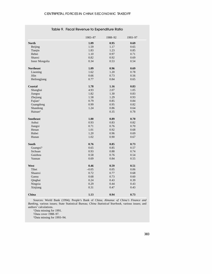
The data on provincial revenue and expenditure indicate a strong positive corre-lation between the provincial revenue to expenditure ratio with per capita income(Table 9). For example, the coastal region and the three municipalities—where percapita incomes are the highest—also have the highest revenue-expenditure ratios. Atthe same time, these ratios are lowest in the western and southern regions, where percapita incomes are also the lowest. This suggests that fiscal policy has also been usedin a redistributive manner.

However, it is important to note several qualifications regarding the provincialfiscal data. First, these data are available only from 1983, and from three differentsources that are occasionally inconsistent for overlapping years.17 Moreover, theydo not appear to include revenue and expenditure by the central government ineach province, which could significantly affect the measurement of the redistribu-tive nature of national fiscal policy. To the extent that such taxation and spendingwere redistributive, their omission from the regression equation could understatethe estimated speed of convergence. Finally, the impact of redistributive fiscalpolicy on growth would depend critically on the form of redistribution. Forexample, the growth implications of income transfers could be very different fromthose associated with infrastructure investment.

III. Estimation Results

The empirical analysis tests for convergence of per capita incomes acrossprovinces by estimating a growth equation that is derived as a log-linear approx-imation of the transition path of per capita output around its steady state level.18

The equation, given below, specifies the average growth rate of per capita outputover the interval t–T and t as a function of initial output and other variables.

ln(yit/yit–T) = C – (1–e–βT) ln(yit–T) + xit + εit, (1)

where i indexes the province, T is the length of the observation interval, t is timeperiod, yit–T is real per capita output at time t–T, the beginning of the subperiod, yit is real per capita income at time t, and β is the convergence coeffi-cient. The convergence coefficient (β) indicates the rate at which yit–T approachesthe steady state level of GDP per capita. A positive coefficient implies that thepoorer provinces grow faster than the richer ones. The higher is β, the more rapidis the convergence to steady state. The variable C is the constant term commonacross provinces, xit includes the vector of other explanatory variables, and εit isan independent error term.

The usual role of the explanatory variables is to capture the structural char-acteristics of the economy that determine the steady state level of per capitaincome. Traditional variables included in the cross-country growth literature are


382

17See Appendix I for a list of the data sources.18The equation for the rate of economic growth is based on the Mankiw, Romer, and Weil (1992)

version of the Solow-Swan model. See also Solow (1956) and Swan (1956).


383

Table 9. Fiscal Revenue to Expenditure Ratio

1983–87 1988–92 1993–97

North 1.09 0.95 0.69Beijing 1.59 1.17 0.65Tianjin 1.83 1.23 0.85Hebei 1.10 0.97 0.71Shanxi 0.82 0.92 0.69Inner Mongolia 0.34 0.53 0.54

Northeast 1.09 0.96 0.69Liaoning 1.62 1.20 0.78Jilin 0.66 0.73 0.56Heilongjiang 0.77 0.84 0.65

Coastal 1.78 1.16 0.83Shanghai 4.93 2.07 1.05Jiangsu 1.82 1.30 0.83Zhejiang 1.58 1.29 0.93Fujian1 0.79 0.85 0.84Guangdong 0.99 0.95 0.82Shandong 1.24 0.86 0.64Hainan2 0.35 0.78

Southeast 1.00 0.89 0.70Anhui 0.93 0.83 0.82Jiangxi 0.71 0.76 0.70Henan 1.01 0.92 0.68Hubei 1.20 0.96 0.69Hunan 1.02 0.90 0.67

South 0.76 0.85 0.73Guangxi3 0.65 0.85 0.57Sichuan 0.93 0.88 0.74Guizhou 0.58 0.76 0.54Yunnan 0.69 0.84 0.55

West 0.46 0.59 0.51Tibet –0.05 0.05 0.06Shaanxi 0.72 0.77 0.68Gansu 0.68 0.73 0.60Qinghai 0.24 0.43 0.39Ningxia 0.29 0.44 0.43Xinjiang 0.31 0.47 0.43

China 1.13 0.94 0.73

Sources: World Bank (1994); People’s Bank of China; Almanac of China’s Finance andBanking, various issues; State Statistical Bureau; China Statistical Yearbook, various issues; andauthors’ calculations.

1Data missing for 1991.2Data cover 1988–97.3Data missing for 1993–94.

the investment rate and educational characteristics. While time series data oneducational characteristics by province or region were not available, we includedthe share of investment to provincial GDP and the private-public mix of produc-tion, as reflected in the share of SOEs in industrial output, in the regressions. Ashighlighted above, the dominance of SOEs in industrial production has variedsharply across the regions. Structural and institutional reforms that improveeconomic incentives and resource allocation and remove impediments to privatesector development are likely to increase the productive capacity of the economyand have an effect on economic growth.19

The remaining variables included in the analysis are policy variables thatappear to be particularly relevant in the Chinese context. These include the shareof FDI flows to provincial GDP, the ratio of revenue to expenditure, and the ratioof bank loans to deposits.20 As noted earlier, higher FDI flows could imply eithermore openness, and thereby a higher rate of convergence, or access to differenttechnology, implying convergence to a different steady state, at least in the shortrun. The rate of convergence would also be affected by the extent of the redis-tributive nature of bank lending and provincial fiscal policies.

The equation is estimated separately for each subperiod (1978–82, 1983–87,1988–92, 1993–97) and for the entire sample period. The estimation results foreach subperiod are based on iterative, nonlinear least squares that allow forheteroskedasticity in the subperiods. For the full sample, the estimates arederived using the seemingly unrelated regression approach (SURE), which alsoallows for correlation of the error terms across the subperiods. For comparison,pooled nonlinear regressions with regional and time dummies were also esti-mated over the corresponding sample period. As shown below, there is littledifference in the full sample estimates except for the estimation results for theperiod 1988–97. Since data on all the explanatory variables are not available forthe entire period, the estimation results are presented for different sample periods(Tables 10, 11, and 12).

Sample Period 1978–97

The first column of Table 10 shows the regression estimates of the convergencecoefficient (β), based on equation (1) where the explanatory variables include onlya constant and the log of each province’s initial per capita income in that subpe-riod. Rows 1–4 of column 1 present the results for each subperiod.

The estimate of β in the first subperiod, 1978–82, is 0.016 or 1.6 percent and ispositively significant. This implies that 1.6 percent of the gap between current output


384

19See Khan (1987) for a review of the nature and evidence for such an effect.20The loan to deposit ratio is intended to capture the redistributive nature of bank lending, or the

extent to which the banking system was a net borrower or net lender in a particular province. Anotherpossibility would be to consider credit availability, measured as the change in real credit, scaled byprovincial GDP. Such a variable would be highly correlated with investment, however, and its construc-tion is complicated by the use of multiple sources of data for bank loans and deposits.

per capita and the steady state per capita output is closed in one year. However, theestimates for the second and third subperiods are insignificant, while the estimatedconvergence coefficient in the fourth subperiod is negatively significant. Large FDIflows, which surged in the fourth period into the northern and coastal regions, maybe viewed as a positive shock that benefited the richer provinces.21 If the estimate ofβ is constrained to be the same for all subperiods, the resulting joint estimate of β is0.001 and is not significant. However, a Wald test for the equality of the coefficientsacross the subperiods rejects the hypothesis that β is stable over the subperiods.


385

Table 10. Estimation Results, 1978–97

(3)

(1) (2) TotalBeta R2 Beta R2 Beta Investment R2

1978–82 0.016* 0.123 0.020* 0.658 0.021* –0.0257 0.66(0.005) 0.086 (0.005) 0.06 (0.006) (0.065) 0.061

1983–87 0.005 0.015 0.018* 0.398 0.017** –0.046 0.402(0.005) 0.078 (0.008) 0.068 (0.010) (0.124) 0.069

1988–92 –0.003 0.009 0.008 0.557 0.007 –0.014 0.558(0.004) 0.072 (0.006) 0.053 (0.007) (0.067) 0.055

1993–97 –0.017* 0.162 –0.004 0.721 0.001 0.056 0.724(0.006) 0.083 (0.007) 0.053 (0.011) (0.106) 0.054

Restricted (SURE) 0.001 0.011** 0.013* 0.062*coefficients (0.003) (0.005) (0.004) (0.029)

Restricted (NLOLS) –0.0002 0.49 0.011* 0.72 0.013* 0.059** 0.73coefficients (0.003) 0.082 (0.004) 0.062 (0.004) (0.034) 0.062

Wald testChi square 24.482 7.142 6.939

Degrees of freedom 3 3 6

p-value 0.000 0.068 0.327

Chi square (0.05) 7.815 7.815 12.592Degrees of freedom 3 3 6

Notes: Standard errors in parentheses; * denotes significance at the 5 percent level, ** at the 10percent level.

21Barro and Sala-i-Martin (1992a) find that the estimated speed of convergence in the U.S. was nega-tive over the period 1920–30. This was attributed to large declines in the relative price of agriculturalcommodities that affected the poorer agricultural states adversely.

Column 2 of Table 10 presents the estimated speed of convergence whenregional dummies are incorporated. These dummies proxy for differences in thesteady state levels of per capita income to which the provinces of China areconverging. Six regional dummies are included for the different regions discussedbefore—the north, northeast, coastal, south, southeast, and west. The inclusion ofregional dummies improves the fit of the estimated equations over the subperiodssuggesting that regional differences are significant.22 The estimated value of theconvergence coefficient over the subperiod 1978–82 increases from 0.016 to 0.02and is positively significant. The estimated coefficient for the subperiod 1983–88also becomes positively significant (β = 0.018). However, the coefficients in thethird and fourth subperiods are insignificant. The estimate of the restricted βincreases to 0.011 or an estimated rate of convergence of 1.1 percent. The Wald testfor equality of the coefficients suggests that the hypothesis of a stable β across thesubperiods can still be rejected at the 5 percent level, but not at the 10 percent level.

In contrast to the Barro and Sala-i-Martin (1991, 1992a, and 1992b) results forU.S. states, Japanese prefectures, and eight European economies, these estima-tions do not provide support for the hypothesis of unconditional convergence.Rather, these results suggest that regions of China are converging to differentsteady state levels of per capita income.

Column 3 of Table 10 includes the ratio of total investment to provincial GDPin the estimations. While this coefficient is not significant for the subperiods, thehypothesis of equality of these coefficients across the subperiods cannot berejected using the Wald test, and the restricted coefficient for total investment ispositively significant. Moreover, the inclusion of this variable affects the estimatedrate of convergence, which increases to 1.3 percent in the combined regression andis now significant at the 5 percent level.23


Since data on FDI flows and revenue and expenditure at the provincial level are notavailable prior to 1983, the relationship between these variables and per capitagrowth was examined over the sample 1983–97.24 Table 11 presents these results.The inclusion of the FDI variable leads to an increase in the estimated rate of conver-gence in the 1983–87 and 1993–97 subperiods. The Wald test again indicates thatthe hypothesis of restricted coefficients over the subperiods cannot be rejected.25


386

22However, these differences do not appear to be significant at the provincial level. Estimations usingfixed effects for each province to test whether each province was converging to its own steady state werenot supported by the data.

23Khan and Kumar (1997) also examine the effect of investment on the speed of convergence for asample of developing countries. They find that the higher the ratio of investment to GDP, the higher is therate of growth of per capita income. The estimated size of the convergence coefficient, taking into accountregional differences, is 1.4 percent, which is very close to the estimated convergence coefficient for China.

24Average levels of the FDI flows over 1985–87 are used for the second subperiod under the assump-tion that the level of FDI flows was close to zero in 1983 and 1984.

25While the estimated coefficients of this equation may, in principle, be affected by collinearitybetween total investment and FDI, there was actually very little correlation between the two variablesover the sample period.

The estimates indicate that FDI flows appear to be positively related to percapita income growth, implying that capital mobility appears to have had a strongeffect on the rate of convergence. The estimated rate of convergence increases to1.8 percent—broadly comparable to results obtained by Barro and Sala-i-Martinof around 2 percent for the U.S., Japan, and Europe. The estimate obtained forChina implies that it takes 38 years to eliminate one-half of the initial gap in percapita incomes.26

The ratio of revenue to expenditure for the provinces appears to have little rela-tion to per capita growth. These results may be due to the problems surrounding theprovincial fiscal data noted above, and to the fact that the ratios used are average


387

Table 11. Estimation Results, 1983–97

(1) (2)

Total TotalBeta Investment FDI R2 Beta Investment FDI Rev/Exp R2

1983–87 0.025* 0.225* 0.020* 0.49 0.034* 0.057 0.019* 0.035 0.51(0.008) (0.080) (0.008) 0.065 (0.009) (0.083) (0.007) (0.025) 0.066

1988–92 0.011 0.003 0.009 0.57 0.011 0.003 0.009 –0.001 0.57(0.008) 0.061 (0.011) 0.055 (0.011) (0.062) (0.011) (0.048) 0.057

1993–97 0.017** 0.128 0.032* 0.78 0.022** 0.175 0.024** 0.081 0.79(0.009) (0.094) (0.011) 0.05 (0.013) (0.116) (0.015) (0.080) 0.05

Restricted (SURE) 0.018* 0.100** 0.019* 0.019* 0.106* 0.019* 0.006coefficients (0.006) (0.055) (0.006) (0.007) (0.053) (0.006) (0.027)

Restricted (NLOLS) 0.020* 0.109* 0.020* 0.74 0.019* 0.109* 0.020* –0.001 0.74coefficients (0.007) (0.055) (0.007) 0.06 (0.007) (0.052) (0.007) (0.024) 0.06

Wald testChi square 6.488 8.83

Degrees of freedom 6 8

p-value 0.371 0.357

Chi square (0.05) 12.592 15.507

Degrees of freedom 6 8

Notes: Standard errors in parentheses; * denotes significance at the 5 percent level, ** at the 10percent level.

26The time t for which log (y(t)) is halfway between log (y(0)) and log (y*) satisfies the conditione–βt = 1/2. The half-life is therefore log(2)/β = 0.69/β. Hence, if β = 0.018, then the half-life is 38 years.


388

Tab

le 1

2.Es

tima

tion

Re

sults

,198

8–97

(1)

(2)

Fixe

d L

oan/

Fixe

dL

oan/

SOE

/B

eta

Inve

stm

ent1

FDI

Dep

osit

R2

Bet

aIn

vest

men

t1FD

ID

epos

itIn

dust

rial

Out

put

R2

1988

–92

0.00

7–0

.082

0.00

1–0

.128

* 0.

670.

006

–0.0

830.

001

–0.1

27*

–0.0

20.

67(0

.006

)(0

.052

)(0

.008

)(0

.039

)0.

05(0

.006

)(0

.051

)(0

.009

)(0

.038

)(0

.030

)0.

051

1993

–97

0.01

70.

104

0.03

3*0.

0001

0.78

0.00

80.

096

0.01

70.

013

–0.0

9*0.

81(0

.014

)(0

.089

)(0

.012

)(0

.041

)0.

052

(0.0

14)

(0.0

87)

(0.0

12)

(0.0

32)

(0.0

32)

0.04

8

Res

tric

ted

(SU

RE

)0.

012*

0.00

7–0

.071

*co

effi

cien

ts(0

.007

)(0

.008

)(0

.027

)

Res

tric

ted

(NL

OL

S)0.

033*

0.23

5*0.

049*

–0.1

13*

0.7

0.01

7**

0.16

*0.

029*

–0.0

72–0

.142

*0.

77co

effi

cien

ts(0

.010

)(0

.070

)(0

.010

)(0

.056

)0.

071

(0.0

10)

(0.0

58)

(0.0

10)

(0.0

52)

(0.0

31)

0.06

3

Wal

d te

stC

hi s

quar

e0.

395

3.62

1 D

egre

es o

f fr

eedo

m1

2

p-va

lue

0.53

00.

164

Chi

squ

are

(0.0

5)3.

841

5.99

1D

egre

es o

ffr

eedo

m1

2

Not

es:S

tand

ard

erro

rs in

par

enth

eses

; * d

enot

es s

igni

fica

nce

at th

e 5

perc

ent l

evel

,**

at th

e 10

per

cent

leve

l.1T

hese

est

imat

ions

use

dat

a on

fix

ed in

vest

men

t ow

ing

to th

e di

verg

ence

in th

e be

havi

or o

f to

tal a

nd f

ixed

inve

stm

ent i

n th

e la

st tw

o su

bper

iods

.

revenue to expenditure rather than marginal revenue to expenditure as mentionedby Jin, Qian, and Weingast (1999). Moreover, revenue contracting practicesbetween different levels of government were subject to frequent negotiation andchange. Institutional changes in 1992–94, which included a shift towards formalfiscal federalism, may also have affected these results.


In order to incorporate data on loan-deposit ratios and the share of SOEs inindustrial output—which are only available from the late 1980s—the regressionswere estimated over a further restricted sample period spanning 1988–97.27 Theconstraints imposed by the small sample period, however, are reflected in theestimation results. The variables appear to behave differently over the twosubperiods 1988–92 and 1993–97. Therefore, the Wald test rejects the hypoth-esis that all coefficients are similar across the subperiods. The results suggestthat the estimate of a stable β coefficient and for the share of SOEs in totalindustrial output across the subperiods cannot be rejected, but the coefficients onthe other variables are different across these periods. These results are shown inTable 12.

In contrast to the FDI flows, the loan-deposit ratio appears to have a nega-tive impact on growth. The loan-deposit ratio is negatively significant over the1988–92 subperiod. This may be due to the fact that SOEs—which faced softbudget constraints and did not invest on purely commercial principles—receivedthe bulk of the credit from state banks. Nonstate enterprises, by contrast,received only limited credit and faced much harder budget constraints. In thelate 1980s and the early 1990s, loans to SOEs accounted for about 80 percent ofall nonagricultural loans, while loans to the nonstate sector consisting of town-ship and village enterprises (TVEs) accounted for only about 8 percent of nona-gricultural loans.28 Hence, the negative relationship between the loan-depositratio and growth could be due to the fact that these transfers tended to supportinefficient SOEs and thereby dampened growth.

If the share of SOEs in total industrial output is included in the estimations,this ratio is negatively significant in the subperiod 1993–97. The negative coef-ficient for the share of SOEs in total output in the pooled estimations alsosuggests that the higher this share, the lower was the rate of economic growth.Hence, the results appear to suggest that enhanced commercial orientation of theSOEs and changes in bank lending policies could have an important positiveeffect on long-run growth.


389

27Instead of total investment in provincial GDP, the share of fixed investment in provincial GDP isused as an explanatory variable as these two measures began to diverge in the 1990s.

28People’s Bank of China (1993).

IV. Conclusions

The estimation results indicate that the regions of China are converging, but todifferent steady state levels of income. The pattern of FDI flows—and the associ-ated technology transfer—appears to have a strong effect on the results. The rela-tively rich coastal and north/northeastern regions, though perhaps more expensive(in terms of labor costs) than the inland regions, were probably able to attract moreFDI precisely because of their relative prosperity and, consequently, more devel-oped infrastructure. The resulting FDI flows boosted the speed of convergence,albeit—at least in the short run—to different steady states for the different regions.

The results suggest that structural characteristics of the regions also appear tohave been important factors determining growth and convergence. For example,the total investment rate appears to be positively correlated with growth, while theprevalence of SOEs and high bank loan-deposit ratios tend to be associated withlower growth. These findings would seem to imply that enhanced commercialorientation of production and the banking system is likely to have a positiveimpact on growth.

The disparity in provincial/regional incomes and the observed convergence todifferent steady states may also be related to the gradual and experimental natureof market-oriented reforms in China. As noted by Bell, Khor, and Kochhar (1993),reform measures tended to be introduced on an experimental basis in some local-ities—often as a result of local initiatives—and expanded to a national scale onlywhen they had proved successful at the local level. The decentralization ofauthority led local governments to assume greater responsibility for state fixedinvestment, initially in industry, but later in infrastructure as well.29 The introduc-tion of agricultural reform and the establishment of special economic zones werealso based on local experimentation. In addition, local governments played animportant role in attracting foreign investment into their localities. Hence, thispattern of development may give rise to strong local effects in the estimationresults. Unless localities within regions tended to adopt reforms at the same time,however, such effects would not be able to explain estimated regional differencesin steady state income levels.

APPENDIX I

Data Sources and Description

Data on provinces’ real and nominal GDP, GDP per capita, agriculture share of GDP, totalinvestment, and fixed investment were taken from The Gross Domestic Product of China,1952–95, and from various issues of the annual China Statistical Yearbook. Provincial popula-tion data were calculated by dividing GDP by GDP per capita; implicit GDP deflators for eachprovince were calculated from the nominal and real GDP series.

Data on provinces’ industrial output, industrial output of SOEs, and foreign direct invest-ment were taken from various issues of the China Statistical Yearbook.


390

29See, for example, Qian (1999), Bell, Khor, and Kochhar (1993), and Tseng and others (1994).

Data on bank deposits and loans in each province were taken from Lardy (1998) for1988–93, and from various issues of the annual Almanac of China’s Finance and Banking for1994–97. Data for 1997 refer only to loans and deposits with the four state commercial banks,which account for around three-quarters of total bank loans and deposits.

Data on provincial revenues and expenditures were taken from World Bank (1994) for1983–90, from various issues of the Almanac of China’s Finance and Banking for 1991–94, andfrom various issues of the China Statistical Yearbook for 1995–97. As noted above, these data donot appear to include central government revenues and expenditures in each province. Moreover,data from the different sources are occasionally inconsistent for years for which overlappingobservations are available.

APPENDIX II

Labor and Capital Mobility

Labor Mobility

The mobility of labor across China’s provinces—and indeed from rural to urban areas withinprovinces—has been limited by policy and institutional factors. Under the household registra-tion system, adopted in 1948, households were designated as either urban or rural; urban house-holds were granted the right to reside in cities and small towns, access to state subsidized grainsupplies, and employment in state enterprises. The 1958 Regulation on the Registration ofHouseholds required households to register their place of residence and to gain permission forany change in residence. Such permission has generally been difficult to obtain.

Following the adoption of agricultural reforms in 1980, rural households’ mobilityincreased somewhat. Communes were disbanded and households no longer had to meet com-mune production quotas. The new household responsibility system allowed rural households todetermine their allocation of labor between farm and nonfarm activities, which in principlemeant that household members could leave the land. However, permission to move under thehousehold registration system remained strictly limited, implying that rural residents could notlegally reside in urban areas. In addition, migration without permission was extremely difficult,as it involved forgoing the benefits that legal residence carried, including food rations, housing,access to schooling for children, and a formal system of old age security. While food and hous-ing have become increasingly available on a market basis over the past decade, unregisteredmigration remains constrained.

Notwithstanding the impediments to urban migration, the number of migrants hasincreased steadily, particularly since the mid-1980s, when the growth in rural incomes began totaper off as the initial boost from rural reforms subsided. Estimates of the total number ofmigrants range from 30 million to 200 million; the World Bank estimated, extrapolating on thebasis of survey data, the total at 40 million in the mid-1990s. This excluded an additional esti-mated 30 million workers who commuted from rural to urban areas on a daily basis.30

The limited mobility of labor has been reflected in data on provinces’ shares in China’stotal population, which have remained virtually unchanged over the past two decades (see Table3). While these data do not capture unregistered migration, much of this has likely been fromrural to urban areas within provinces rather than across provinces. Hence, such migration is notlikely to have altered the provincial population shares in a substantial manner.


391

Capital Mobility

In addition to limiting the mobility of labor, government policies have, in effect, had a damp-ening impact on the mobility of capital across provinces. Empirical evidence supports thehypothesis that interprovincial capital mobility has indeed been limited.

Tax policies

The profit retention system, which was in place in the early 1980s, discouraged regional capi-tal mobility.31 Under this system, enterprises’ transfers to other locations resulted in a loss inprofits accruing to the local government, as retained profits were part of local revenue. In1983–84, modifications to the revenue-sharing system—which involved the decentralization ofplan formulation, lowering of plan production targets, and permission to sell above plan outputon the market—resulted in a sharp increase in enterprise investment, although the incentive toretain funds within local jurisdictions remained high.

In the late 1980s, following the introduction of the contract responsibility system, whichfixed profit remittances by enterprises, and a system of revenue-sharing between different lev-els of government, localities have increasingly offered incentives to attract investment. Indeed,according to the World Bank (1994), there has been a proliferation of tax exemptions offeredby localities once they have arranged to fulfill their revenue target specified in the contract withthe level of government directly above.32 As a result, the interregional capital mobility that doestake place is based on tax differentials rather than differentials in resource endowments or costadvantages.

Empirical tests of capital mobility

Empirical evidence presented by Zhao (1998) supports the view that the degree of capitalmobility within China is limited, and that the interprovincial capital flows that have taken placehave not generally reflected optimizing behavior by investors seeking to equalize rates of returnon investment. The empirical tests are based on the proposition that, under perfect capitalmobility, an increase in a province’s saving rate should be reflected in an increase in allprovinces’ investment rates, since saving would flow to all provinces to equalize the rates ofreturn on investment.

Zhao (1998) finds that the correlation between provinces’ saving and investment rates havegenerally been high, suggesting that capital has not been freely mobile across provinces. Thehigh correlations remain even after adjusting for the effect of common factors on saving andinvestment rates. Zhao also finds that correlations were somewhat lower in provinces where theshare of investment in the state enterprise sector was large, suggesting that the capital that movedacross provincial boundaries was that of the state-owned sector, in which optimizing investmentdecisions are likely to have played a relatively small role. Conversely, in provinces with the high-est shares of private investment in total investment—such as the coastal provinces—the correla-tion between saving and investment rates was particularly high. Adjusting for this effect, thedegree of integration—capital mobility—across provinces is small.


392

30World Bank (1997). Jian, Sachs, and Warner (1996) estimate the total number of migrants at100–150 million.

31A detailed discussion of the institutional aspects of taxation policy and its effect on interregionalcapital mobility is contained in World Bank (1994).

32The World Bank (1994) estimates that there were 1,800 special zones granting tax concessions atthe county level or above in early 1993.

REFERENCES

Aziz, Jahangir, and Christoph Duenwald, 2001, “China’s Provincial Growth Dynamics,” IMFWorking Paper 01/3 (Washington: International Monetary Fund).

Barro, Robert J., and Xavier Sala-i-Martin, 1991, “Convergence Across States and Regions,”Brookings Papers on Economic Activity, 1, pp. 107–82 (Washington: BrookingsInstitution).

———, 1992a, “Convergence,” Journal of Political Economy, Vol. 100 (April), pp. 223–51.

———, 1992b, “Regional Growth and Migration: A Japan-United States Comparison,” Journalof Japanese and International Economics, Vol. 6 (December), pp. 312–46.

———, 1995, Economic Growth (New York: McGraw-Hill).

Bell, Michael W., Hoe Ee Khor, and Kalpana Kochhar, 1993, China at the Threshold of aMarket Economy, IMF Occasional Paper 107 (Washington: International Monetary Fund).

Ben-David, Dan, 1993, “Equalizing Exchange: Trade Liberalization and Income Convergence,”Quarterly Journal of Economics, Vol. 108 (August), pp. 653–79.

Cashin, Paul, and Ratna Sahay, 1996, “Internal Migration, Center-State Grants, and EconomicGrowth in the States of India,” IMF Staff Papers, Vol. 43 (March), pp. 123–71.

Graham, Edward M., and Erika Wada, 2001, “Foreign Direct Investment in China: Effects onGrowth and Economic Performance” (unpublished; Washington: Institute for InternationalEconomics).

Husain, Aasim M., 1998, “Economic Performance and Business Cycles in China’s Provincesand Regions,” in People’s Republic of China: Selected Issues (Washington: InternationalMonetary Fund).

Khan, Mohsin S., 1987, “Macroeconomic Adjustment in Developing Countries: A PolicyPerspective,” World Bank Research Observer, Vol. 2, pp. 23–42.

Khan, Mohsin S., and Manmohan Kumar, 1997, “Public and Private Investment and the GrowthProcess in Developing Countries,” Oxford Bulletin of Economics and Statistics, Vol. 59, pp.69–88.

Jian, Tianlun, Jeffrey D. Sachs, and Andrew M. Warner, 1996, “Trends in Regional Inequalityin China,” NBER Working Paper 5412 (Cambridge, Massachusetts: National Bureau ofEconomic Research).

Jin, Hehui, Yingi Qian, and Barry R. Weingast, 1999, “Regional Decentralization and FiscalIncentives: Federalism, Chinese Style” (unpublished; Stanford, California: StanfordUniversity).

Lardy, Nicholas, 1998, China’s Unfinished Economic Revolution (Washington: The BrookingsInstitution).

Mankiw, N. Gregory, David Romer, and David N. Weil, 1992, “A Contribution to the Empiricsof Economic Growth,” Quarterly Journal of Economics, Vol. 107 (May), pp. 407–37.

People’s Bank of China, various issues, Almanac of China’s Finance and Banking (Beijing:China Financial Publishing House).

Qian, Yingyi, 1999, “The Institutional Foundations of China’s Market Transition,” paperprepared for the Annual World Bank Conference on Development Economics, WashingtonDC, April 28–30.

Quah, Danny, 1997, “Empirics for Growth and Distribution: Polarization, Stratification, andConvergence Clubs,” Journal of Economic Growth, Vol. 95 (December), pp. 27–59.

Solow, Robert M., 1956, “A Contribution to the Theory of Economic Growth,” QuarterlyJournal of Economics, Vol. 70, pp. 65–94.


393

State Statistical Bureau, 1996, The Gross Domestic Product of China, 1952–95 (Beijing: ChinaStatistical Publishing House).

———, various issues, China Statistical Yearbook (Beijing: China Statistical Publishing House).

Swan, Trevor W., 1956, “Economic Growth and Capital Accumulation,” Economic Record,Vol. 32, pp. 334–61.

Tseng, Wanda, Hoe Ee Khor, Kalpana Kochhar, Dubravko Mihaljek, and David Burton, 1994,Economic Reform in China: A New Phase, IMF Occasional Paper 114 (Washington:International Monetary Fund).

Wei, Shang-Jin, and Yi Wu, 2001, “Globalization and Inequality: Evidence from Within China”(unpublished; Washington: International Monetary Fund).

World Bank, 1994, “China: Budgetary Policy and Intergovernmental Fiscal Relations”(Washington: World Bank).

———, 1997, “Income Distribution in China,” China and Mongolia Department (Washington:World Bank), June.

Zhao, Rui, 1998, “Capital Mobility and Regional Integration: China 1978–95” (unpublished;Washington: International Monetary Fund).


394

Centripetal Forces in China’s Economic Takeoff ... · Centripetal Forces in China’s Economic...

Documents

Transcript of Centripetal Forces in China’s Economic Takeoff ... · Centripetal Forces in China’s Economic...