CENTRE FOR ECONOMETRIC ANALYSIS

CEA@Cass

http://www.cass.city.ac.uk/cea/index.html

Cass Business School

Faculty of Finance

106 Bunhill Row

London EC1Y 8TZ

Money Market Funds, Shadow Banking and

Systemic Risk in United Kingdom

Carlo Bellavite Pellegrini, Michele Meoli and Giovanni Urga

CEA@Cass Working Paper Series

WP–CEA–03-2017

1

Money Market Funds, Shadow Banking and Systemic Risk in United Kingdom1

Carlo Bellavite Pellegrini†, Michele Meoli**,c, Giovanni Urga***

This version: 13 January 2017

Abstract

Shadow banking entities have been repeatedly charged with the breaking up of the recent financial

crises. This paper examines the contribution of the money market funds, an important part of the

shadow banking entities, to the systemic risk in United Kingdom by using the CoVaR methodology

(Adrian and Brunnermeier, 2016). Using a sample of 143 money market funds, continuously listed

between 2005Q4 and 2013Q4, we investigate the impact of institutional corporate variables on the

systemic risk. Our results show that liquidity mismatch increases the average systemic risk over the

whole period, but decreases the risk during the Great Financial Depression.

Keywords: Money Market Funds, Shadow banking, Global Financial Crisis, Panel Data. J.E.L. Classification: G01, G15, G21, G23, C23. †Department of Economics and Business Management Sciences, and Research Centre of Applied Economics, Catholic University, Milan (Italy) ** Department of Management, Information and Production Engineering, University of Bergamo (Italy), and CCSE, University of Bergamo (Italy) *** Faculty of Finance, Cass Business School, City University of London (UK), and Department of Management, Economics and Quantitative Methods, University of Bergamo, (Italy) c: contact author.

1 We wish to thank participants in the Centre for Econometric Analysis Occasional Seminar on “Shadow Banking, Financial Instability and Monetary Policy” (6 November 2015, Cass Business School, London) in particular Thorsten Beck, Barbara Casu, Angela Gallo, Ian Marsh, the Banca IMI Research Seminar (21 October 2016, Milan), in particular Massimo Baldi e Massimo Mocio, and the Bank of England Research Seminar (9 November 2016, London) in particular Evangelos Benos, Nicola Garbarino and Daniele Massacci for helpful comments and suggestions. Special thanks to Barbara Casu for very useful comments to a previous version of this paper. We wish to thank the Editor-in-Chief, Brian Lucey, and an anonymous referee for very useful comments that helped to improve the paper. The usual disclaimer applies. We acknowledge financial support from the Bank of England Research Donation Committee (RDC201410), the Centre for Econometric Analysis, Cass Business School, London, and the Centre for Studies in Applied Economics (CSEA) - Catholic University of Milan, and Banca IMI, Milan.

2

1. Introduction

Financial literature has recently devoted an increasing attention to the issue of shadow banking,

exploring institutional features in the United States (Poszar et al. 2012, Adrian and Ashcraft 2016),

United Kingdom (Jackson 2013), and the Euro area (Bakk-Simon et al. 2012).

In particular, the supposed involvement in the triggering of the recent financial crisis2 has been

investigated by considering the relationships between shadow banking and the traditional banking

system during the financial crisis (Hsu and Moroz 2010, Meeks, et al. 2014). The main differences

between the two lie in the distinction between relationship based lending versus actuarially based

lending (Hancock and Passmore 2015) and the nature of core liabilities in the traditional banking

system versus the noncore liabilities in the shadow banking system (Harutyunyan et al. 2015).

Despite the significant bulk of research dedicated to this issue, many distinguishing features of the

shadow banking activities are still unexplored, and an empirical assessment of their contribution to

systemic risk is yet to come.

In particular, Money Market Funds (MMFs henceforth), ascribed by financial literature as a part

of the external and independent shadow banking entities, according to the definition introduced by

Poszar (2008), Poszar et al. (2012) and Adrian and Ashcraft (2016), and representing a significant

part of the listed shadow banking entities, have been often criticized for having contributed to

spread systemic risk. Kodres (2015) notices that during the crisis we observed runs - not the usual

retail runs but wholesale funding runs - on MMFs that had provided funding to commercial and

universal banks (both in United States and in Europe).

MMFs are collective investment schemes which invest in “money market” instruments, with a

very negligible risk, such as short-term high credit quality and liquid debt instruments, government

securities, commercial paper, certificates of deposit and short-term securities or provide repurchase

agreement (repo) financing. The returns to investors in the mutual fund are a straightforward

function of the gain and losses of the mutual fund’s investment portfolio. Money market mutual

funds are a sort of “open end” funds in which investors get back their funds redeeming their shares3.

The main aim of this paper is to identify the main determinants of MMFs contribution to

systemic risk. There are several reasons of why focusing on MMFs is of interest. On the one hand,

these shadow entities are directly involved in a revised form of risk and maturities transformation, 2 According to The Economist’(10/5/2014, p. 9), Mark Carney, Governor of the Bank of England and head of the Financial Stability Board (FSB), identifies the shadow banking in emerging markets as “the greatest danger to the world economy”. 3 The value of a share in a mutual fund can be identified in the “Net Asset Value” of the fund. The Net Asset Value of a mutual fund is the net value of all of its assets divided by the number of shares outstanding. Thus the NAV approximates the liquidation value of an investor’s shares in a fund. It is the price at which investors can buy fund shares or sell them back to the fund. The fund managers calculates the NAV of the fund each day, and when an investor wants his money back, the fund buys (or redeems) the investor’s shares at the price per share (Macey, 2011).

3

and are therefore likely to be identified as financial devices potentially increasing systemic risk of

the financial sectors. On the other hand, they are typically seen as entities with very negligible risk,

because their assets are not characterized by maturity mismatch. Therefore, following the arguments

in previous literature (Macey 2011; Kodres 2015), in this paper we investigate whether the liquidity

mismatch characterizing these entities lead to a positive or negative contribution to systemic risk,

discriminating what we can observe during ordinary periods or during financial crises.

To this purpose, in this paper we adopt the Conditional Value-at-Risk (CoVaR) measure

introduced by Adrian and Brunnermaier (2016). The CoVaR quantifies the contribution of a

financial institution to systemic risk and its contribution to the risk of other financial institutions.

CoVaR indicates the Value-at-Risk (VaR) of financial institution i, conditional on financial

institution j being in distress. Adrian and Brunnermeier (2016) argue that this is a more complete

measure of risk since it is able to capture alternative sources of risk which affect institution i even

though they are not generated by it. Furthermore, if we consider that institution i is the whole

financial system, then ΔCoVaR is defined as the difference between the CoVaR and the

unconditional VaR and it captures the marginal non-causal contribution of a particular institution to

the overall systemic risk.

In this paper, we build on the CoVaR methodology, which allows us to generate time-varying

estimates of the systemic risk contribution of MMFs as a specific sector of the financial industry.

We employ micro data from 143 MMF listed on the London Stock Exchange from 2005Q4 to

2013Q4 While our time span allows us to cover the different phases of the recent financial crises,

namely the Subprime crisis and the Great Financial Depression, the United Kingdom’s context is

chosen because it represents one of the most developed shadow banking system among the

European countries with a relevant presence of listed money market funds.

To anticipate some findings, our empirical applications allow us to identify what institutional

features of shadow entities are correlated to systemic risk. As a contribution to previous literature,

we find that liquidity mismatch plays a major role as determinant of ΔCoVaR: it increases systemic

risk over the whole period, while mitigates risk during the Great Financial Depression.

The reminder of the paper is organised as follows. Section 2 describes the nature and the main

features of the shadow banking system and its relationship with the systemic risk literature. Section

3 introduces the methodology and the data used in our analysis. Section 4 reports the main

empirical findings. Section 5 concludes.

4

2. The contribution of MMFs to systemic risk

2.1 Shadow banking entities and systemic risk

One of the main challenges of recent financial literature on the topic has consisted in the

identification of shadow banking activities and of features that banks do not have.

Even if “shadow banks are easier to define by what they are not than by what they are” (The

Economist, Special Report International Banking, May 10th 2014), recent banking and financial

literature provides different definitions of shadow banking. McCulley (2007) introduces the notion

of shadow banking as an unregulated financial institution characterized by high leverage without to

benefit from a safety net or other official guarantees. According to Adrian and Ashcraft (2016), the

shadow banking system is a web of specialized financial institutions that conduit funding from

savers to investors through a range of securization and secured funding techniques, while Claessens

and Ratnovski (2014) define shadow banking as all financial activities, except traditional banking,

requiring a private or public backstop to operate. For Mehrling et al. (2013) shadow banking is

simply money market funding of capital market lending, sometimes on the balance sheets of entities

called banks and sometimes on their balance sheets. Moreover, the Financial Stability Board (2011)

defines the shadow banking system as the system of credit intermediation that involves entities and

activities outside the regular banking system. In addition, revealing its prejudice about the role of

shadow banking in financial turmoil, it states that shadow banking encompasses all financial

activities and entities that increased systemic risk owing to maturity/liquidity transformation and/or

leverage and/or showing indications of regulatory arbitrage as well.

This issue has been developed by the Poszar’s (2008) and Poszar et al. (2012), providing a

classification of the different natures and features of shadow banking entities. The authors define

shadow banking as a chain of financial intermediaries that conduct credit intermediation,

decomposing the same credit intermediation “into a chain of wholesale-funded, securitization-based

lending” and defining seven steps of shadow bank credit intermediation. Moreover, Pozsar et al.

(2012) identifies for different kind of shadow banking. The first is defined as internal shadow

banking and consists of activities that are conducted by subsidiaries of banking holding. Hence

these activities are included in the traditional banking’s structure. For instance, a banking holding

company may own wealth management unit or may provide liquidity to entities belonging to

shadow banking system. Moreover, in many cases the largest non-bank subsidiaries of banking

groups are finance companies, broker-dealers and wealth management unit, such as mutual funds,

hedge fund and money market funds. For these reasons, the authors stress that the shadow banking

system is organized around securitization and wholesale funding. The second category,

denominated as external shadow banking, consists of independent and regulated institutions that

5

conduct shadow banking activities, but these do not represent their primary business. They refer to

stand-alone broker-dealers, independent wealth management institutions, credit hedge funds and

finance companies, like auto loan subsidiaries. The third category, defined as independent shadow

banking, consists of entities which are specialized only in shadow banking, such as structured

investment vehicle, stand-alone money market funds, independent collateralized debt obligation,

collateralized debt obligation and the majority of asset backed securities. The fourth group, defined

as government sponsored shadow banking, includes government-sponsored enterprises, such as

Fannie Mae and Freddie Mac in the United States (see also the European Commission 2012).

These four categories are partially overlapping because, for example, a money market fund may

be ascribed to the first typology as a subsidiary of a banking holding, or to the third one, being an

independent entity, potentially listed, and involved in shadow banking activity.

From the overview of the definitions of shadow banking, an important issue clearly emerges. In

comparison with the traditional banking system, shadow banking would transform risk and

maturities (Diamond and Dybvig 1983) without the presence of direct and explicit public sources of

liquidity and of any sort of public deposit insurance (Adrian and Ashcraft 2016). This fact

suggested that shadow banking is intrinsically fragile (Pozsar et al. 2012), and is at the basis of the

exploratory researches analysing the relationship with systemic risk, as in Duca (2015), stressing

the role of reserve and other regulatory requirements that induced shifts from bank loans to other

sources of finance, boosting shadow banking activity in the past decade.

2.2 Money Market Funds and their contribution to Systemic Risk

The financial literature highlights, within the shadow banking sector, the wholesale funding

channel as one of the potential device triggering systemic risk (Paltalidis et al. 2015). For this

reasons, Poschmann (2012) focuses on mutual funds, money market funds, hedge funds and finance

companies like consumer and commercial finance companies, leasing companies and factors or

captive financing subsidiaries of non-financial corporations like auto or equipment lease financing

related. The main mission of these companies is to provide loans to consumers and businesses;

therefore, they are important suppliers of credit. Finance companies do not take deposits from

public as funding source, but they issue commercial paper and other short and medium term debt

instruments in order to raise funds. The increasing relevance of the above mentioned typologies of

shadow banking entities is witnessed by Jackson (2013) who highlights that in Europe many small

and medium enterprises are principally financed by leasing and factoring companies rather than

traditional banks. Thus, it is reasonable to assume that the above described typologies of shadow

6

banking entities, involved in a revised form of transforming risk and maturities, may be ascribed as

financial devices potentially increasing systemic risk of the financial sectors.

We focus our attention on continuously listed money market funds, being a part of “external and

independent” listed shadow banking entities: they are linked with the systemic risk issue and it is

possible to obtain reliable data of corporate variables both in accounting and financial measures.

The main aim of this study is to test whether money market funds have contributed to increase

systemic risk or to decrease systemic risk. The theoretical argument follows Hsu and Moroz (2010),

suggesting that the liquidity mismatch does not necessarily imply that the assets have longer term

than liabilities. For example, a money market fund can be compelled to a fire sale of assets, because

of a request of an immediate liability redemption. In other words, money market funds do not have

any problems connected with the existence of a maturity mismatch between assets and liabilities,

because they do not have liabilities as the commercial banks financing the assets, but investors’

shares. Conversely money market funds may experience an issue linked with liquidity mismatch in

periods of financial crisis, because they could not have an immediate cash availability to tune the

request of an investors’ shares redemption with the sale of assets on the market. Therefore, while

their liquidity mismatch can generally add to systemic risk in ordinary conditions, a reverse effect is

likely to be observed in periods of crisis, such as during the recent Great Financial Depression.

We can formalize our expectation as follows:

Hypothesis 1: The higher is the liquidity mismatch of a MMF, the higher will be the

contribution to systemic risk.

Hypothesis 2: During a financial crisis, the higher is the liquidity mismatch of a MMF, the

lower will be the contribution to systemic risk.

2. Methodology and Data

Our paper makes use of the CoVaR measure of Adrian and Brunnermeier (2016). The most

common measure of risk used by financial institutions is the value-at-risk (VaR), which focuses on

the risk of an individual institution in isolation. The q%-VaR is the maximum dollar loss within the

q%-confidence interval. Formally, the q-VaR for an institution i can be defined as:

𝑃𝑃𝑃𝑃𝑃𝑃𝑃𝑃(𝑋𝑋𝑖𝑖 ≤ 𝑉𝑉𝑉𝑉𝑉𝑉𝑞𝑞𝑖𝑖 ) = 𝑞𝑞% (1)

7

where 𝑋𝑋𝑖𝑖 is the variable of institution i for which the 𝑉𝑉𝑉𝑉𝑉𝑉𝑖𝑖 is defined that we set 𝑋𝑋𝑖𝑖 to be the

growth rates of market-valued total financial assets. Note that 𝑉𝑉𝑉𝑉𝑉𝑉𝑖𝑖 is typically a negative number

and, while in practice the sign is often switched, we will not follow this convention, in accordance

to Adrian and Brunnermeier (2016).

The indicator of systemic risk, 𝐶𝐶𝑃𝑃𝑉𝑉𝑉𝑉𝑉𝑉, is defined as the 𝑉𝑉𝑉𝑉𝑉𝑉 of the financial system as a whole

conditional on some event C(Xi) of institution i. That is, 𝐶𝐶𝑃𝑃𝑉𝑉𝑉𝑉𝑉𝑉𝑞𝑞𝑠𝑠𝑠𝑠𝑠𝑠𝑠𝑠𝑠𝑠𝑠𝑠|𝐶𝐶(𝑋𝑋𝑖𝑖) is defined by the q-th

quantile of the conditional probability distribution:

𝑃𝑃𝑃𝑃𝑃𝑃𝑃𝑃(𝑋𝑋𝑠𝑠𝑠𝑠𝑠𝑠𝑠𝑠𝑠𝑠𝑠𝑠|𝐶𝐶(𝑋𝑋𝑖𝑖) ≤ (𝐶𝐶𝑃𝑃𝑉𝑉𝑉𝑉𝑉𝑉𝑞𝑞𝑠𝑠𝑠𝑠𝑠𝑠𝑠𝑠𝑠𝑠𝑠𝑠|𝐶𝐶(𝑋𝑋𝑖𝑖)) = 𝑞𝑞% (2)

where 𝑋𝑋𝑖𝑖 is the market-valued asset return of institution i, and 𝑋𝑋𝑠𝑠𝑠𝑠𝑠𝑠𝑠𝑠𝑠𝑠𝑠𝑠 is the return of the portfolio,

computed as the average of the 𝑋𝑋𝑖𝑖’s weighted by the lagged market value assets of the institutions

in the portfolio. Adrian and Brunnermeier (2016) measure the contribution of each single institution

to systemic risk by the ΔCoVaR, namely the difference between CoVaR conditional on the

institution being in distress and CoVaR in the median state of the institution.

As far as the estimation method is concerned, quantile regressions are employed to estimate

CoVaR. First, one can estimate the predicted value of a quantile regression where the financial

sector losses 𝑋𝑋𝑞𝑞𝑠𝑠𝑠𝑠𝑠𝑠𝑠𝑠𝑠𝑠𝑠𝑠|𝑋𝑋𝑖𝑖 is determined given the losses of a particular institution i for the q%-

quantile:

𝑋𝑋�𝑞𝑞𝑠𝑠𝑠𝑠𝑠𝑠𝑠𝑠𝑠𝑠𝑠𝑠|𝑋𝑋𝑖𝑖 = 𝛼𝛼�𝑞𝑞𝑖𝑖 + �̂�𝛽𝑞𝑞𝑖𝑖 𝑋𝑋𝑖𝑖 (3)

where 𝑋𝑋�𝑞𝑞𝑠𝑠𝑠𝑠𝑠𝑠𝑠𝑠𝑠𝑠𝑠𝑠|𝑋𝑋𝑖𝑖 denotes the predicted value for a particular q%-quantile of the system conditional

on a return realization 𝑋𝑋𝑖𝑖 of institution i. From the definition of VaR, in equation (1), we have that:

𝑉𝑉𝑉𝑉𝑉𝑉𝑞𝑞𝑠𝑠𝑠𝑠𝑠𝑠𝑠𝑠𝑠𝑠𝑠𝑠|𝑋𝑋𝑖𝑖 = 𝑋𝑋�𝑞𝑞

𝑠𝑠𝑠𝑠𝑠𝑠𝑠𝑠𝑠𝑠𝑠𝑠|𝑋𝑋𝑖𝑖 (4)

In practice, the predicted value from the quantile regression of the system losses on institution i

losses gives the value at risk of the financial system conditional on 𝑋𝑋𝑖𝑖, because the 𝑉𝑉𝑉𝑉𝑉𝑉𝑞𝑞𝑠𝑠𝑠𝑠𝑠𝑠𝑠𝑠𝑠𝑠𝑠𝑠|𝑋𝑋𝑖𝑖 is

simply the conditional quantile. Using the particular predicted value of 𝑋𝑋𝑖𝑖 = 𝑉𝑉𝑉𝑉𝑉𝑉𝑞𝑞𝑖𝑖 yields the

𝐶𝐶𝑃𝑃𝑉𝑉𝑉𝑉𝑉𝑉𝑞𝑞𝑖𝑖 measure. More formally, within the quantile regression framework, the 𝐶𝐶𝑃𝑃𝑉𝑉𝑉𝑉𝑉𝑉𝑞𝑞𝑖𝑖 measure

is:

8

𝐶𝐶𝑃𝑃𝑉𝑉𝑉𝑉𝑉𝑉𝑞𝑞𝑖𝑖 = 𝑉𝑉𝑉𝑉𝑉𝑉𝑞𝑞𝑠𝑠𝑠𝑠𝑠𝑠𝑠𝑠𝑠𝑠𝑠𝑠|𝑋𝑋𝑖𝑖=𝑉𝑉𝑉𝑉𝑉𝑉𝑞𝑞𝑖𝑖 = 𝛼𝛼�𝑞𝑞𝑖𝑖 + �̂�𝛽𝑞𝑞𝑖𝑖 𝑉𝑉𝑉𝑉𝑉𝑉𝑞𝑞𝑖𝑖 (5)

The Δ𝐶𝐶𝑃𝑃𝑉𝑉𝑉𝑉𝑉𝑉𝑞𝑞𝑖𝑖 is therefore given by:

Δ𝐶𝐶𝑃𝑃𝑉𝑉𝑉𝑉𝑉𝑉𝑞𝑞𝑖𝑖 = 𝐶𝐶𝑃𝑃𝑉𝑉𝑉𝑉𝑉𝑉𝑞𝑞𝑖𝑖 − 𝐶𝐶𝑃𝑃𝑉𝑉𝑉𝑉𝑉𝑉50𝑖𝑖 = �̂�𝛽𝑞𝑞𝑖𝑖 (𝑉𝑉𝑉𝑉𝑉𝑉𝑞𝑞𝑖𝑖 − 𝑉𝑉𝑉𝑉𝑉𝑉50𝑖𝑖 ) (6)

In order to simplify the notation, in what follows q is always set to be 5%, so that CoVaRi

identifies the system losses predicted on the 5% loss of institution i, while ΔCoVaRi identifies the

deterioration in the system losses, when the institution i moves from its median state to its 5% worst

scenario.

These measures are defined as time-varying, and in practice, in order to estimate the time-

varying VaRt¸ as in equation (3) and CoVaRt,, as in equation (5), we include a set of state variables

to capture the time variation in conditional moments of asset returns. With references to these

specific market’s factors, we also follow the implementation adopted by Lopez-Espinosa et al.

(2012) to take into account the peculiarities of the European institutional environment. In practice,

in our analysis we use the following variables:

1. FTSE-Vol: is the weekly price of the index of the FTSE 100 as a volatility index; ii)

2. Liquidity Spread: is the liquidity spread calculated as the difference between the three months

UK repo rate and the three months UK T bill;

3. T-bill change: indicates the change in UK T bill 3-month rate;

4. Y-Curve slope: indicates the change in slope of the yield curve represented by UK 5-year

minus three-months interest rate on government bonds;

5. Credit spread: indicates the change in credit spread represented by the difference between

BBB corporate bonds and the ten year German government bonds;

6. Equity Return: indicates the weekly equity returns from the FTSE 100.

Our analysis is performed on a sample of 143 British MMF continuously listed between

2005Q4 and 2013Q4, thus covering the Subprime Crisis and the Great Financial Depression. Table

1 shows the total market capitalization of the sample. Over the period 2005Q4-2013Q4, money

market funds represent an average capitalization of roughly 76% of listed shadow banking entities

in the United Kingdom, being the remaining part constituted by finance companies. In terms of

capitalization the whole sector was severely hit between 2007 and 2009 by the Great Financial

9

Depression, registering in 2011 the recovery of 2007’s market capitalization and a further

significant increase since then.

[INSERT HERE TABLE 1]

Table 2 reports the mean, median, minimum, maximum and standard deviation values of 95%-

risk measures, computed for 143 entities on weekly data for the period 2005Q4-2013Q4 and

financial market losses X(i). Indicating with 𝑀𝑀𝑀𝑀𝑠𝑠𝑖𝑖 the market value of a money market fund and

with 𝐿𝐿𝑀𝑀𝑉𝑉𝑠𝑠𝑖𝑖 the ratio between total assets and common equity, we can define:

𝑋𝑋𝑖𝑖 = 𝑀𝑀𝑀𝑀𝑡𝑡𝑖𝑖×𝐿𝐿𝑀𝑀𝑉𝑉𝑡𝑡

𝑖𝑖−𝑀𝑀𝑀𝑀𝑡𝑡−1𝑖𝑖 ×𝐿𝐿𝑀𝑀𝑉𝑉𝑡𝑡−1

𝑖𝑖

𝑀𝑀𝑀𝑀𝑡𝑡−1𝑖𝑖 ×𝐿𝐿𝑀𝑀𝑉𝑉𝑡𝑡−1

𝑖𝑖 (7)

where the sum of all the 𝑋𝑋𝑖𝑖 of the sample gives𝑋𝑋𝑠𝑠𝑠𝑠𝑠𝑠𝑠𝑠𝑠𝑠𝑠𝑠, namely the growth rate of the market value

of the total asset of financial sector under analysis. The values of VaR are obtained by performing

the quantile regressions (95%) of weekly lagged returns of market variables and computing the

expected value of the regression. The CoVaR is the expected value of the quantile regression (95%)

of the capital losses of the financial system on the financial losses of the individual institution and

delayed market variables. The ΔCoVaR is the difference between the CoVaR with a quantile

regression to 95% and that to 50%.

Table 2 shows that money market funds of our sample went through some turbulent period.

Indeed, during 2005Q4 and 2013Q4, the VaR was almost equal to -2% (on average), while the

CoVaR and ∆CoVaR were equal to -2.1% and -2%, respectively. However, whenever we observe

the values of the same quantities for the European traditional banking (Bellavite Pellegrini et al.

2015), we find a different picture: i.e the VaR is equal to -9% (on average), CoVaR equal to -5.2%

(on average) and a ∆CoVaR equal to -3.6%, which are considerably larger values than those found

for the UK money market funds.

[INSERT HERE TABLE 2]

Once estimated the ΔCoVaR, our analysis implies the identification of the institutional

determinants correlated. For the U.K. money market funds, we take into analysis the corporate

variables as described by Adrian and Brunnermaier (2016) and by Lopez Espinosa et al. (2012) and

adapt them to the money market funds specificities. For this mentioned reason we take into

10

consideration a modified variable of maturity mismatch and we define it as “liquidity mismatch”, as

mentioned above, according to (Hsu and Moroz 2010; Poschmann 2012), as an effective main

potential source of systemic risk.

1. Leverage indicates the leverage calculated as the total assets to equity ratio of the money

market fund i at quarter (t-1);

2. Liquidity Mismatch indicates the relative level of short term funding as the total short term

debt minus cash to total liabilities ratio of money market fund i at quarter (t-1);

3. ERV indicates the equity return volatility;

4. Beta is the equity market beta ;

5. M-t-B is the market to book ratio of money market fund i at quarter (t-1);

6. Size represents the total assets of money market fund i at quarter (t-1).

In Table 3, we report the descriptive statistics both for the institutional variables and for the

state variables to capture the time variation in conditional moments of asset returns. If we compare

the values with those of the UK traditional banking system (as reported in Bellavite Pellegrini et al.

2014), we notice that the average value of leverage, 1.54, is more than ten times lower than the

traditional banking system one of 22.34, while the liquidity mismatch experiences a negative value

of -3.70 which may be only partially compared with the maturity mismatch for the traditional

banking system which shows a value of 7.17. Only a slight difference arises regarding the market to

book value being 0.94 for money market funds as compared to 1.01 for the traditional UK banking

system, while the beta coefficient in the traditional banking system is 1.26, which is more than

double than in our money market funds of 0.56.

[INSERT HERE TABLE 3]

3. Empirical Results

We estimate a panel predictive regression model with fixed effects, where the full

specification can be described as follows:

∆𝐶𝐶𝑃𝑃𝑉𝑉𝑉𝑉𝑉𝑉𝑖𝑖𝑠𝑠 = 𝛽𝛽𝑖𝑖0 + 𝛽𝛽1∆𝐶𝐶𝑃𝑃𝑉𝑉𝑉𝑉𝑉𝑉𝑖𝑖𝑠𝑠−1 + 𝛽𝛽2𝑉𝑉𝑉𝑉𝑉𝑉𝑖𝑖𝑠𝑠−1 + 𝛽𝛽3𝐿𝐿𝐿𝐿𝐿𝐿𝐿𝐿𝑃𝑃𝑉𝑉𝐿𝐿𝐿𝐿𝑖𝑖𝑠𝑠−1 + 𝛽𝛽4𝑀𝑀𝑀𝑀𝑖𝑖𝑠𝑠−1 + 𝛽𝛽5𝑀𝑀𝑉𝑉𝑉𝑉𝑖𝑖𝑠𝑠−1 +

𝛽𝛽6𝐵𝐵𝐿𝐿𝐵𝐵𝑉𝑉𝑖𝑖𝑠𝑠−1 + 𝛽𝛽7𝑀𝑀𝐵𝐵𝑉𝑉𝑖𝑖𝑠𝑠−1+𝛽𝛽8𝑆𝑆𝑆𝑆𝑆𝑆𝐿𝐿𝑖𝑖𝑠𝑠−1 + 𝛽𝛽𝑐𝑐1𝐶𝐶𝑃𝑃𝑆𝑆𝐶𝐶𝑆𝑆𝐶𝐶1 + 𝛽𝛽𝑐𝑐2𝐶𝐶𝑃𝑃𝑆𝑆𝐶𝐶𝑆𝑆𝐶𝐶2 +

∑ 𝛽𝛽𝑘𝑘𝑇𝑇𝑆𝑆𝑇𝑇𝐿𝐿𝑘𝑘 + 𝜀𝜀𝑖𝑖𝑠𝑠𝑠𝑠−1𝑘𝑘=1 (8)

11

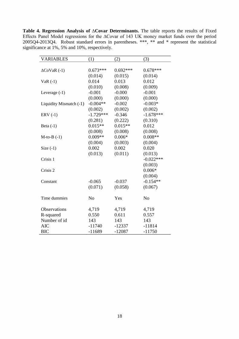
Table 4 reports the results of several estimated equations, where the specification described

above has been simplified according to the following rules. Column (1) represents our baseline

specification considering the full sample period, without crisis and time dummies. In column (2),

we report the regression containing time dummies. Specification (3) considers crisis dummies: in

particular, the dummy variable Crisis 1 captures the characteristics of the Subprime Crisis,

containing period between the outbreak of subprime loans crisis in 2007Q3 and the outbreak of

crisis in 2008Q3; the dummy variable Crisis 2 captures the effects of the Global Financial Crisis

running since 2008Q4 (the bankruptcy of Lehman Brothers) to 2010Q2.

[INSERT HERE TABLE 4]

Model (1) highlights that equity return volatility has a negative and statistically significant

impact on systemic risk, meanwhile liquidity mismatch has a negative impact on systemic risk. This

latter results confirms our Hypothesis 1. As far as the other corporate variables are concerned,

money market funds’ beta and market to book value are likely to mitigate systemic risk. Model (2)

confirms former finding when controlling for time-specific effects. Model (3) documents a negative

and statistically significant impact of the dummy Crisis 1 while Crisis 2 dummy has a positive

impact. This latter finding suggests that money market funds have contributed to decrease and not

to increase systemic risk during the Global Financial Crisis in United Kingdom, being otherwise

their role much more detrimental during the Subprime Crisis. In broad terms, Black et al. (2013)

document a similar result about the contribution of the British banking system to the systemic risk

of the European ones.

Table 5 reports the marginal effect of money market funds corporate variables over Crisis 1 and

Crisis 2. Column (4) reports the main coefficients, while column (5) and column (6) report the

marginal effects, i.e. the interactions between the money market funds’ corporate variables and

Crisis 1 and Crisis 2, respectively.

[INSERT HERE TABLE 5]

The results listed in Column (5) show that none of the money market funds corporate variables

was moderated by the Subprime Crisis, while Column (6) reports a positive impact of liquidity

mismatch and beta coefficient on systemic risk during the Global Financial Crisis. This results

12

confirms our Hypothesis 2, and represent a contribution with respect to former literature, where the

maturity mismatch is identified as negatively related to risk, especially in a context of crisis. Indeed,

empirical evidence on traditional banking (Bellavite Pellegrini et al. 2015; Betz et al., 2016),

suggests that the traditional banking system maturity mismatch represents a proxy of

interconnectedness among financial institutions, being extremely beneficial in normal times and

very detrimental during the financial turmoil. As far as the shadow entities are concerned, Hsu and

Moroz (2010) stress that money market funds liquidity mismatch has not too much to share with

traditional banks maturity mismatch, because it does not imply that assets have a longer average

duration than liabilities. A money market funds has to sell off its assets whenever none of the

liabilities can be rolled over.

The different results that we report with respect to MMFs may be interpreted according to the

different institutional features of liquidity mismatch for money market funds and for maturity

mismatch in the traditional banking system. In this respect, Table 2 shows how the average value of

liquidity mismatch for money market funds is negative and how these entities are featured by a low

level of leverage. If we combine these two pieces evidence, it emerges that money market funds are

characterized by the existence of a potentially satisfying level of liquidity. For money market funds,

this corporate variable is likely to represent a proxy of liquidity endowment which is useful in

lowering systemic risk during the financial turmoil. Similar evidence occurs for the beta coefficient

being likely to respectively decrease systemic risk in the Great Financial Depression for money

market funds and to increase for traditional banks.

4. Conclusions

This paper evaluated the impact of the corporate variables of 143 continuously listed money

market funds, a considerable part of shadow banking entities, on systemic risk in United Kingdom

over the period 2005Q4-2013Q4 covering both the Subprime Crisis and the Great Financial

Depression. Corporate and financial descriptive statistics suggest that UK money market funds are

featured by an average value of leverage more than ten times lower as compared with traditional

UK banks, as well as by a negative average value for the liquidity mismatch. An important result of

our study is related to the different impact of liquidity mismatch on systemic risk on the whole

period and during the Global Financial Crisis, being first negative (implying increasing systemic

risk) and the second positive (decreasing systemic risk). As comparison, the results for the

European traditional banking system reported by Bellavite Pellegrini, et al. (2015) show that

maturity mismatch have an opposite impact. In this respect, UK listed money market funds are

likely to have decreased rather than increased systemic risk during the Global Financial Crisis.

13

These results are confirmed when we introduce in our specification two Crisis dummies,

documenting a negative impact during the Subprime Crisis and a positive impact during the Global

Financial Crisis. Most likely this finding depends on the different endowment of liquidity of these

entities had in comparison with traditional banks.

It will be interesting to extend this research to other shadow banking entities, such as finance

companies for instance, also considering other European countries, in particular continental Europe.

We leave this development to future research.

14

References

Adrian, T., Ashcraft, A. B., 2016. Shadow banking: a review of the literature. In (ed) Garett Jones, Banking Crises Perspectives from the New Palgrave Dictionary of Economics, Palgrave Macmillan UK, 282-315.

Adrian T., Ashcraft A. B. and Cetorelli, N., 2013. Shadow banking monitoring. Federal Reserve Board of New York Staff Report N. 638. Adrian, T., Brunnermeier, M., 2016. CoVar. American Economic Review. 106 (7), 1705-1741. Bakk-Simon K., Borgioli S., Giron C., Hempell H., Maddaloni A., Recine F., Rosati S., 2012. Shadow Banking in the Euro Area. An Overview. European Central Bank, Occasional Paper Series N. 133. Bellavite Pellegrini C., Meoli M., Urga G. e Pellegrini L., 2015. Systemic Risk of European Banks over the period 2006-2012 in (eds) G. Bracchi and D. Masciandaro, Reshaping Commercial Banking in Italy: New Challenges from Lending to Governance, Edibank Bancaria, Gruppo ABI, 203-214. Betz, F., Hautsch, N., Peltonen, T. A., Schienle, M., 2016. Systemic risk spillovers in the European banking and sovereign network. Journal of Financial Stability 25, 206-224. Claessens S., Ratnovski L., 2015. What is Shadow Banking? in “Shadow Banking Within and across National Borders” (eds) Claessens, S., Evanoff, D., Kaufman, G., Laeven, L. World Scientific, 405-412 Duca, J.V., 2015. What Drives Shadow Banking? Evidence from Short-Term Business Credit” in (eds) Claessens, S., Evanoff, D., Kaufman, G., Laeven, L., Shadow Banking Within and Across National Borders, World Scientific, 1001-121 Duca, J.V., 2015. How capital regulation and other factors drive the role of shadow banking in funding short-term business credit. Journal of Banking and Finance, 69, S10-S24. Diamond, D. W., Dybvig, P. H., 1983. Bank runs, deposit insurance, and liquidity. The Journal of Political Economy, 91, 401-419. Eijffinger Sylvester C.W., 2009. Defining and Measuring Systemic Risk. European Parliament. Available at: www.europarl.europa.eu. European Commission 2012. Green Paper Shadow Banking. COM(2012) 102 final. Financial Stability Board 2011. Shadow Banking: Strengthening Oversight and Regulation. Recommendations of the Financial Stability Board. Gorton G., Metrick A., 2010. Haircuts. Federal Reserve Bank of St. Louis Review 92(6).

15

Hancock, D. Passmore, W., 2015. Traditional banks, shadow banks, and financial stability in (eds) Claessens, S., Evanoff, D., Kaufman, G., Laeven, L., Shadow Banking Within and across National Borders.World Scientific, 67-79. Harutyunyan, A. Massara, A., Ugazio, G., Amidzic, G., Walton, R., 2015. Shedding light on shadow banking. International Monetary Fund Working Paper 15/1.

Hsu, J. C. and Moroz, M., 2010. Shadow Banks and the Financial Crisis of 2007-2008 in (ed) Greg Gregoriou, The Banking Crises Handbook, CRC Press (2009), 39-56. Jackson P., 2013. Shadow Banking and New Lending Channels – Past and Future in 50 Years of Money and Finance: Lessons and Challenges, SUERF- The European Money and Finance Forum, Larcier, Vienna. Kodres, L.E., 2015. Shadow banking - What are we really worried about?” in (eds) Claessens, S., Evanoff, D., Kaufman, G., Laeven, L., Shadow Banking Within and Across National Borders, World Scientific., 229-237 Lopez-Espinosa G., Moreno A., Rubia, A., Valderrama L., 2012. Short-term wholesale funding and systematic risk: a global CoVaR approach. Journal of Banking and Finance, 36, 3150-3162. Macey, J. R., 2011. Reducing Systemic Risk: The Role of Money Market Mutual Funds as Substitutes for Federally Insurance Bank Deposits. John M. Olin Center for Studies in Law, Economics and Public Policy, Research Paper N. 422. Mehrling, P., Pozsar, Z., Sweeney, J., Neilson, D. H., 2013. Bagehot was a shadow banker: shadow banking, central banking, and the future of global finance. Available from SSRN: http://ssrn.com/abstract=2232016. Meeks, R., Nelson, B. D., and Alessandri, P., 2014. Shadow banks and macroeconomic Instability. Bank of England Working Paper N. 487. McCulley P., 2007. Teton Reflections. PIMCO Global Central Bank Focus. Paltalidis, N., Gounopoulos, D., Kizys, R., & Koutelidakis, Y., 2015. Transmission channels of systemic risk and contagion in the European financial network. Journal of Banking & Finance, 61, S36-S52. Poschmann J., 2012. The shadow banking system - Survey and typological framework. Working Papers on Global Financial Markets N. 27. Pozsar Z., 2008. The rise and fall of the shadow banking system. Moodys Economy.com. Pozsar Z., Adrian T., Ashcraft A., Boesky H., 2012. Shadow banking. Federal Reserve Bank of New York Staff Report N. 458.

.

16

TABLES

Table 1. Market capitalization for the full sample of money market funds (mln £). The table reports the average market capitalization, calculated year by year, for the sample of 143 money market funds continuously listed in the UK over the period 2005Q4-2013Q4.

Capitalization/Years 2005 2007 2009 2011 2013

Money market funds 30,263.00 41,275.90 29,272.29 39,291.51 46,448.25

Table 2. Summary Statistics. The table reports the average and median values, and the standard deviation of the corporate variables, for the sample of 143 money market funds continuously listed in the UK between 2005Q4 and 2013Q4, and of the variables used to estimate the ∆CoVaR, calculated over the period 2005Q4-2013Q4.

Average Median Standard

Deviation

Leverage 1.547 1.101 6.679

Liquidity Mismatch -3.704 -0.104 32.768

ERV 0.013 0.011 0.007

Beta 0.568 0.577 0.353

M-t-B 0.948 0.900 0.906

Size (mln£) 212.439 184.427 109.737

FTSE-Vol 0.012 0.010 0.006

Liquidity Spread 0.086 0.073 0.070

T-Bill Change -0.010 -0.002 0.049

Credit Spread 2.687 2.714 0.555

Y-Curve Slope 0.005 0.003 0.034

Equity Return 0.009 0.026 0.076

17

Table 3. Summary Statistics for X(i), VaR, CoVaR and ∆CoVaR. The table reports average, median, min and max values, standard deviation, for the growth rate in market value of the total asset (X(i)), for the Value at Risk (VaR), for the CoVaR and the ∆CoVaR measures, calculated for the 143 money market funds listed in UK over the period 2005Q4-2013Q4.

Average Median Minimum Maximum Standard Deviation

X(i) 0.00173 0.00116 -32.242 61.409 0.2878

VaR -0.0173 -0.0103 -32.242 12.662 0.1379

CoVaR -0.0213 -0.02145 -0.2663 0.4236 0.0157

∆CoVaR -0.0196 -0.0185 -0.2304 0.39123 0.01540

18

Table 4. Regression Analysis of ∆Covar Determinants. The table reports the results of Fixed Effects Panel Model regressions for the ∆Covar of 143 UK money market funds over the period 2005Q4-2013Q4. Robust standard errors in parentheses. ***, ** and * represent the statistical significance at 1%, 5% and 10%, respectively.

VARIABLES (1) (2) (3) ∆CoVaR (-1) 0.673*** 0.692*** 0.678*** (0.014) (0.015) (0.014) VaR (-1) 0.014 0.013 0.012 (0.010) (0.008) (0.009) Leverage (-1) -0.001 -0.000 -0.001 (0.000) (0.000) (0.000) Liquidity Mismatch (-1) -0.004** -0.002 -0.003* (0.002) (0.002) (0.002) ERV (-1) -1.729*** -0.346 -1.678*** (0.281) (0.222) (0.310) Beta (-1) 0.015** 0.015** 0.012 (0.008) (0.008) (0.008) M-to-B (-1) 0.009** 0.006* 0.008** (0.004) (0.003) (0.004) Size (-1) 0.002 0.002 0.020 (0.013) (0.011) (0.013) Crisis 1 -0.022*** (0.003) Crisis 2 0.006* (0.004) Constant -0.065 -0.037 -0.154** (0.071) (0.058) (0.067) Time dummies No Yes No Observations 4,719 4,719 4,719 R-squared 0.550 0.611 0.557 Number of id 143 143 143 AIC -11740 -12337 -11814 BIC -11689 -12087 -11750

19

Table 5. Regression Analysis of ∆Covar Determinants (Marginal effects for money market funds over the financial crisis). The table reports the results of a Fixed Effects Panel Model regression for the ∆Covar of the 143 UK money market funds over the period 2005Q4-2013Q4. Column (4) reports the baseline coefficients, Column (5) the coefficients of the variables interacted with Crisis 1, and Column (6) the coefficients of the variables interacted with Crisis 2. Robust standard errors in parentheses. ***, ** and * represent the statistical significance at 1%, 5% and 10%, respectively.

(4) (5) (6)

VARIABLES Baseline coefficients

Marginal effects over Crisis 1

Marginal effects over Crisis 2

∆CoVaR (-1) 0.666*** 0.095*** 0.000 (0.018) (0.023) (0.024) VaR (-1) -0.008 0.003 0.035** (0.011) (0.025) (0.016) Leverage (-1) -0.002** -0.005 0.004 (0.001) (0.005) (0.003) Liquidity Mismatch (-1) -0.006*** 0.013 0.012*** (0.002) (0.027) (0.004) ERV (-1) -1.687*** -0.757 -0.050 (0.355) (0.550) (0.501) Beta (-1) 0.009 0.019 0.022* (0.008) (0.013) (0.013) M-to-B (-1) 0.017** -0.005 -0.024 (0.008) (0.014) (0.015) Size (-1) 0.020 0.004 -0.007 (0.012) (0.006) (0.008) Crisis 1 -0.015 (0.033) Crisis 2 0.054 (0.040) Constant -0.060* (0.036) Observations 4,719 R-squared 0.562 Number of id 143 AIC -11828 BIC -11662

20

Appendix

Table A1. Average and median values of balance sheet variables by year (mln £). The table reports the average and median values of some balance sheet values, calculated year by year for the sample of 143 money market funds listed in UK over the period 2005Q4-2013Q4.

2005 2007 2009 2011 2013 Total Asset

Average 268.33 353.81 259.12 338.00 398.16 Median 143.42 177.80 126.17 180.05 202.81

Common Equity Average 235.29 317.52 227.16 299.32 355.81 Median 114.07 158.08 114.07 158.84 175.35

Short Term Debt Average 6.92 10.23 7.34 13.33 15.59 Median 0.05 1.41 - 0.37 4.15

Cash&Equivalent Average 11.20 14.65 16.38 15.31 17.37 Median 3.03 2.90 3.93 3.45 3.10

Total Liabilities Average 31.72 35.03 30.68 38.60 42.20 Median 12.76 12.70 9.42 11.29 14.66