ISA Transactions 52 (2013) 149–161

Contents lists available at SciVerse ScienceDirect

ISA Transactions

0019-05

http://d

n Corr

E-m

journal homepage: www.elsevier.com/locate/isatrans

Practice Article

Centralized and distributed control architectures under FoundationFieldbus network

Maria Auxiliadora Muanis Persechini n, Fabio Gonc-alves Jota

Department of Electronics Engineering, Federal University of Minas Gerais, Av. Antonio Carlos, 6627. Belo Horizonte, MG 31.270-901, Brazil

a r t i c l e i n f o

Article history:

Received 9 February 2012

Received in revised form

29 August 2012

Accepted 19 September 2012Available online 18 October 2012

This paper was recommended for

publication by Rickey Dubay

Keywords:

Automation system architecture

Process Control

Fieldbus network

Control Performance Assessment

78/$ - see front matter & 2012 ISA. Published

x.doi.org/10.1016/j.isatra.2012.09.005

esponding author.

ail address: dorap@ufmg.br (M.A.M. Persechin

a b s t r a c t

This paper aims at discussing possible automation and control system architectures based on fieldbus

networks in which the controllers can be implemented either in a centralized or in a distributed form.

An experimental setup is used to demonstrate some of the addressed issues. The control and

automation architecture is composed of a supervisory system, a programmable logic controller and

various other devices connected to a Foundation Fieldbus H1 network. The procedures used in the

network configuration, in the process modelling and in the design and implementation of controllers

are described. The specificities of each one of the considered logical organizations are also discussed.

Finally, experimental results are analysed using an algorithm for the assessment of control loops to

compare the performances between the centralized and the distributed implementations.

& 2012 ISA. Published by Elsevier Ltd. All rights reserved.

1. Introduction

Automation systems are responsible for the operation, monitoringand control of industrial processes. Features of these systems alsoinclude the ability for optimization, scheduling and planning. Auto-matic control requires that all sub-systems perform, safely andefficiently, all the functions that are essential to operate theprocess [1]. Nevertheless, the reliability and performance char-acteristics depend, in general, on the system architecture (i.e., thelogical organization of its components and the associated infra-structure). Thus, the choice of the components determines itsmain features such as reliability, product quality, performance,scalability and cost. Therefore, the selection of a specific archi-tecture is not trivial and depends, for example, on the processtype, the operating procedures, the instrumentation, the controland the management systems used.

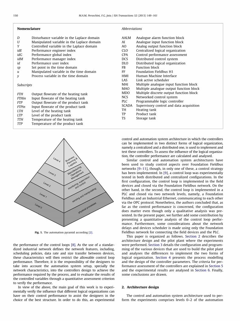
System architectures for process control and automation arehierarchically organized complex structures. Based on CIM (Com-puter Integrated Manufacturing) model, these structures aredesigned in different levels [2]. Level 0 defines the actual physicalprocesses, Level 1 defines the activities involved in sensing andmanipulating the physical processes variables, Level 2 defines theactivities of monitoring, supervisory control and automated con-trol of the production process, Level 3 defines the ManufacturingOperations Management systems and Level 4 defines the Business

by Elsevier Ltd. All rights reserve

i).

Planning and Logistics systems. This hierarchical structure as shownin Fig. 1 is usually referred to as the automation pyramid.

The system architecture infrastructure is responsible for con-necting and integrating the automation pyramid levels in order toexchange information effectively and consistently by using dif-ferent networks technology. Some of these networks, generallyreferred to as fieldbus networks are being widely used on fieldinstruments in the process industries [3–5].

In general, fieldbus networks are connected to other devices suchas programmable logic controllers (PLC) and computers to build theinfrastructure necessary to implement the process automation andcontrol functions. In industry, it is common to find fieldbus networksconnected to a special PLC card which, in turn, interconnects the PLCto computers that perform supervision systems. In this case, sensorsand actuators are connected to the controllers by the fieldbusnetwork, being the control algorithms executed in the PLC in acentralized logical organization. However, depending on the type ofthe fieldbus network employed, the field devices may execute thecontrol algorithm in a distributed logical organization. Therefore,when using fieldbus networks, in either distributed or centralizedlogical organization, the exchange of data between the sensor, thecontroller and the actuator requires communications via network as anetworked control system (NCS).

Various ways of closing the feedback control system via acommunication network have been widely investigated but thestability and performance of the closed-loop system will alwaysbe limited by the network characteristics [6,7]. Typical para-meters of NCS, such as scheduling schemes, maximum delays andthe number of packet dropouts, can impose severe limitations on

d.

Nomenclature

D Disturbance variable in the Laplace domainU Manipulated variable in the Laplace domainY Controlled variable in the Laplace domainidE Performance engineer indexidG Performance global indexidM Performance manager indexid Performance user indexsp Set point in the time domainu Manipulated variable in the time domainy Process variable in the time domain

Subscripts

FTH Output flowrate of the heating tankFTHin Input flowrate of the heating tankFTP Output flowrate of the product tankFTPin Input flowrate of the product tankLTH Level of the heating tankLTP Level of the product tankTTH Temperature of the heating tankTTP Temperature of the product tank

Abbreviations

AALM Analogue alarm function blockAI Analogue input function blockAO Analog output function blockCLO Centralized logical organizationCPA Control performance assessmentDCS Distributed control systemDLO Distributed logical organizationFB Function blockFF Foundation Fieldbus H1HMI Human Machine InterfaceLAS Link active schedulerMAI Multiple analogue input function blockMAO Multiple analogue output function blockMDO Multiple discrete output function blockNCS Networked control systemPLC Programmable logic controllerSCADA Supervisory control and data acquisitionTH Heating tankTP Product tankTS Storage tank

Fig. 1. The automation pyramid according [2].

M.A.M, Persechini, F.G, Jota / ISA Transactions 52 (2013) 149–161150

the performance of the control loops [8]. As the use of a standar-dized industrial network defines the network features, including,scheduling policies, data rate and size transfer between devices,these characteristics will then restrict the allowable control loopperformance. Therefore, it is the responsibility of the designers totake into account the automation system setup, specially thenetwork characteristics, into the controllers design to achieve theperformance required by the process, and to evaluate the results ofthe controlled variables through a quantitative assessment criterionto verify the performance.

In view of the above, the main goal of this work is to experi-mentally verify the influence that different logical organizations canhave on their control performance to assist the designers in thechoice of the best structure. In order to do this, an experimental

control and automation system architecture in which the controllerscan be implemented in two distinct forms of logical organization,namely a centralized and a distributed one, is used to implement andtest these controllers. To assess the influence of the logical organiza-tion, the controller performance are calculated and analysed.

Similar control and automation system architectures havebeen used to study control aspects over Foundation Fieldbusnetworks [9–11], though, in only one of these, a control strategyhas been implemented. In [9], a control loop was experimentallytested in both distributed and centralized configurations. In thefirst configuration, the control loop is implemented in the fielddevices and closed via the Foundation Fieldbus network. On theother hand, in the second, the control loop is implemented in aPLC and closed via two network levels, namely, a FoundationFieldbus and an Industrial Ethernet, communicating to each othervia the OPC protocol. Nonetheless, the authors concluded that, asfar as the control performance is concerned, the configurationdoes matter even though only a qualitative analysis was pre-sented. In the present paper, we further add some contribution bypresenting a quantitative analysis of the control loop perfor-mance. Furthermore, some considerations about the networkdelays and devices scheduler is made using only the FoundationFieldbus network for connecting the field devices and the PLC.

This paper is organized as follows. Section 2 describes thearchitecture design and the pilot plant where the experimentswere performed. Section 3 details the configuration and program-ming of the various devices that are used to build the pilot plantand analyses the differences to implement the two forms oflogical organization. Section 4 presents the process modellingand the design of the controller parameters. The criteria for per-formance assessment of the controllers are explained in Section 5and the experimental results are analysed in Section 6. Finally,some conclusions are drawn.

2. Architecture design

The control and automation system architecture used to per-form the experiments comprises levels 0–2 of the automation

Fig. 2. Pilot plant control and automation architecture.

Fig. 3. Diagram of the pilot plant.

M.A.M, Persechini, F.G, Jota / ISA Transactions 52 (2013) 149–161 151

pyramid. This system is composed of a pilot-scale plant, representa-tive of an industrial continuous process, instrumented with com-mercial devices (such as sensors, actuators and controllers) andsoftware applications that are also commonly used in industries.Also, using the same hardware infrastructure the controllers can beimplemented in either centralized or distributed logical organization.

Fig. 2 shows the control and automation architecture used toperform the experiments and details to these architecture areexplained in the next sections.

2.1. Pilot plant

The pilot plant used in the experiments presented in the paper,shown in Fig. 3, is a system composed of three interconnectedtanks of water (a storage tank, TS, with a storage capacity of 500 l;a heating tank, TH, of 50 l; and a product tank, TP, of 75 l).The water is pumped from TS to TH and to TP by pump B-1, and,from TP to TS, by the pump B-2. The water flows naturally bygravity from TH to TP. The water flowrate from TS to TH ismeasured by FT1, from TH to TP by FT2, from TS to TP by FT3 andfrom TP to TS by FT4. The level and temperature of TH arerespectively measured by LT1 and TE1, and the level and tem-perature of TP are respectively measured by LT2 and TE2. The righas also four control valves: TCV1 installed on the piping betweenTH and TP, FCV1 installed on the piping between TP and TS, LCV1installed on the piping between TS and TH and LCV2 installed onthe piping between TS and TP. Finally, there is a heating system atthe bottom of TH manipulated by a 4–20 mA signal from TTC1.

2.2. Instrumentation

As shown in Fig. 2, a Foundation Fiedbus H1 (hereafter onlyreferred to as FF) network is chosen for real-time data commu-nication between sensors, actuators and controllers. In this case,the FF devices function blocks can be configured allowing dis-tributed control implementation. Analyses of FF networks havebeen presented elsewhere; for example, in [12–15], the effects ofdelays introduced by the FF network are analysed and, in [16,17],techniques for the scheduling policy of the messages on thenetwork are discussed. Furthermore, some examples of applica-tions are reported [18–20]. However, details of the schedulingalgorithms and of the network layer implementation are notavailable for commercial devices. This hinders a theoretical modeldevelopment and a priori evaluation of network communicationseffects on the control system.

As regard to the pilot plant, Fig. 3, the field instruments areconnected by a FF network. As shown in Fig. 2, levels (LT1 andLT2) and flowrates (FT1, FT2, FT3 and FT4) are measured by sixLD032 devices, and temperatures (TE1 and TE2) are measured byone TT302 device. Since the signal sent to the control valves andto the heating system varies in the range of 4–20 mA, there aretwo FI302 devices to convert the FF network signal into a4–20 mA signal. One of the FI302 devices sends signals to thevalves TCV1 and FVC1 and the other sends signals to the heatingsystem TTC1 and to the valves LCV1 and LCV2. The devices LD302,TT032 and FI302 are manufactured by [21] and are easily found inindustries.

2.3. Monitoring and control

In this paper, the infrastructure for monitoring and control iscomposed of one PLC and one computer running a SCADA(supervisory control and data acquisition) system to performthe HMI. As shown in Fig. 2, the PLC is connected to the computervia a serial RS232 port communicating to each other via theModbus protocol. The PLC is also connected to the FF network byusing an interface card, FB700. This card is used for exchangingdata between the PLC and the FF network. A PLC digital outputcard controls the drives of the pumps B-1 and B-2 . A specialdevice, Foundation Fieldbus Universal Bridge DFI302, performsthe Link Active Scheduler (LAS) of the FF network and allows the

Fig. 4. Control strategy diagram.

M.A.M, Persechini, F.G, Jota / ISA Transactions 52 (2013) 149–161152

connection of the FF network to the computer using a High SpeedEthernet (HSE) network.

For developing the control strategies, the computer runs thesoftware applications required to configure the FF network and toprogram the PLC. To monitor and to operate the pilot plant, thecomputer also runs a SCADA system and data acquisition softwarefor historical records. These application softwares are OPC clientsthat communicate with two OPC servers, one of them for the FFnetwork and the other for the PLC, both servers running on thecomputer.

2.4. Control strategy

The architecture of the control and automation of the pilot plant,as seen in Fig. 2, allows the implementation of different controlstrategies. In this case, five control loops were implemented byusing a multiloop control strategy. For the first loop, the controlledvariable yLTH(t) that varies in the range of 0–440 mm, is the TH levelmeasured by LT1, and the manipulated variable uLTH(t) is the signalsent to the control valve LCV1. For the second loop, the controlledvariable yLTP(t) that varies in the range of 0–650 mm, is the TP levelmeasured by LT2 and the manipulated variable uLTP(t) is the signalsent to the control valve LCV2. For the third loop, the controlledvariable yFTP(t) that varies in the range of 0–52 l/min, is theTP output flowrate measured by FT4 and the manipulated variableuFTP (t) is the signal sent to the control valve FCV1. For the fourthloop the controlled variable yTTP(t) that varies in the range of theambient temperature (approximately 22 1C) to 60 1C, is the TPtemperature measured by TE2 and the manipulated variable uTTP(t)is the signal sent to the control valve TCV1. For the fifth loop thecontrolled variable yTTH(t) that varies in the range of the ambienttemperature (approximately 22 1C) to 70 1C, is the TH temperaturemeasured by TE2 and the manipulated variable uTTH(t) is the signalsent to the heating system TTC1. All the manipulated variables varyin the range of 0–100 %. In addition, the water flowrates measuredby FT1, FT2, and FT3 are respectively monitored by the variablesyFTHin(t), yFTH(t), and yFTPin(t).

For the purposes of this work, the TP output flowrate and theTP and TH level control loops are operated in automatic mode,whereas the TP and TH temperature control loops are operated inmanual mode.

The TP output flowrate and the TP and TH level control loopscan be implemented by using different strategies. Both the CLPand the FF network devices have different features that can beused to implement the control strategy. However, the FF networkdevices do not have a programming language such as the PLC; inthis case, the control strategy is implemented by connecting thestandard function blocks, making it impractical to implementadvanced control strategies such as adaptive control, multivari-able and robust control. On the other hand, those advancedstrategies can be implemented in the CLP provided that it hasenough memory and a suitable programming language (forexample, structured text). Since this papers’ goal is to comparethe performance of centralized and distributed logical organiza-tions, the same control strategy should be implemented in bothorganizations. In this case, one common feature is the use of thePID controllers that can be organized in a multiloop controlconfiguration with the possibility of adding additional decouplerscontrollers or feedforward controllers.

Fig. 4 presents the block diagram of the control system empha-sizing the transfer functions used to represent the dynamics of theTP output flowrate and TP and TH levels. In this figure, KLTP(s),KLTH(s) and KFTP(s) are three PID controllers for controlling respec-tively the TP level, the TH level and the TP output flowrate; K13 andK24 are feedforward controllers designed to reduce respectively theload disturbances caused by uFTP(t) on yLTP(t) and by uTTP(t) on

yLTH(t); and gij(s) are transfer functions on the Laplace domain thatrepresent the dynamic behaviour of the controlled variables.

The choice of this structure was dictated by different reasons.First, tests demonstrated that interactions between loops aresignificant, suggesting the use of decoupling controllers. Second,a feedback control combined with a feedforword control is asimple and efficient structure for decoupling control loops widelyused in industries. Finally, the controller type is limited by thedevices used in the pilot plant, especially the FF instrumentswhose PID equation is

UðsÞ ¼ Kp EðsÞ�sTd

1þasTdYðsÞþ

EðsÞ

sTi

� �þKff Uff ðsÞ ð1Þ

where Kp, Ti and Td are respectively the proportional, the integraland the derivative term, U(s) is the manipulated variable, Y(s) isthe controlled variable, E(s) is the difference between the setpoint and the controlled variable, Kff is a feedforword controllergain and Uff(s) is the variable that caused the disturbance.

3. System configuration

The control strategy, as shown in Fig. 4, is implemented by usingtwo different logical organizations: the distributed one and thecentralized one, hereafter referred to as DLO and CLO respectively.The FF network devices, shown in Fig. 2, are then configured, and thestandard function blocks (FBs) inside the devices are parametrized.The PLC is programmed using ladder language. To allow the user to

Fig. 5. Synoptic diagram to operate and monitor the pilot plant.

M.A.M, Persechini, F.G, Jota / ISA Transactions 52 (2013) 149–161 153

operate and monitor the pilot plant, some synoptic diagrams, as forexample the one shown in Fig. 5, were properly constructed in theSCADA application. The procedures to implement the control strat-egy using the FF devices and the PLC are explained in the sequel.

3.1. Distributed logical organization

Fig. 6(a) shows a scheme of the FBs connections used toimplement the DLO strategy. In this design, the AI (analogue input),AO (analogue output) and PID FBs are connected for controlling TPand TH levels and temperatures, and TP output flowrate. The FFnetwork devices are also configured to set digital alarms to informlow and high levels of TH and TP; high temperature of TH and TPand high flowrate of TP output. These alarms are generated bycomparing the values of the AI FBs to the default down and upperlimits values using AALM (analogue alarm) FBs. Since the heater andthe pumps B-1 and B-2 are commanded by the PLC digital outputcard, the digital alarms are transferred from the FF devices to thePLC by the FB700 interface card using a MDO (multiple discreteoutput signals) FB.

With regard to the block diagram shown in Fig. 4, the PID FBsthat run the controllers according to Eq. (1) are allocated in the FFnetwork sensors: KLTP(s) and K13 are run by the LD302-LT1 sensorto control the TH level, KLTH(s) and K24 are run by LD302-LT2sensor to control the TP level, and KFTP(s) is run by LD302-FT4sensor to control TP output flowrate.

There is a recommendation given by the FF devices suppliersthat the PID FB should be located at the same device running theAO block so as to reduce the number of external links and thusminimizing the overall execution time of the network. However,there is only one PID block in each device. As shown in Fig. 2, oneof the FI302 device has two AO blocks and the other three AOblocks. Since there are five control loops and only one PID in eachFI302 device, this recommendation could not be implemented.Therefore, the PID FBs for the three control loops under analysis(TP output flowrate and TP and TH levels) are located in the sameLD302 devices that run the AI blocks, so that these control loopshave the same number of external links.

To ensure the safe operation of the pilot plant, the PLC isprogrammed to turn off the heater and the pumps according tothe alarm values set by the FF devices and to receive the turn on/off user commands from the SCADA application.

3.2. Centralized logical organization

To implement the control strategy in the centralized form theinterface card (FB700) that connects the PLC to the FF network isconfigured to read the AI FB values from the FF devices and towrite the AO FB values according to the PLC program results. Thisinterface card must to be configured for both the FF network andthe PLC. For the FF network, the FB700 is configured with a MAI(multiple analogue input) FB and a MAO (multiple analogueoutput) FB, as shown in Fig. 6(b). The MAI receives, from the FFnetwork devices, the AI FB values measured by TE1, TE2, FT1, FT2,FT3, FT4, LT1 and LT2; and the MAO sends, to the AO FBs, thevalues to manipulate the valves LCV1, LCV2, FCV1 and TCV1 andto the heating system TTC1.

On the PLC side, the interface card is configured as a virtualanalogue input module that corresponds to the MAI FB and as avirtual analogue output module card, corresponding to the MAOFB, so that the AI FB values and the AO FB values correspondrespectively to the PLC’s analogue input variables and outputanalogue variables.

The PLC programming includes the five control loops (TP andTH levels and temperatures as well as TP output flowrate) and thesetting of the digital alarms using the input and output analoguevariables. It also controls the pumps and the heater (turning themon or off according to the alarm sates or the SCADA commands).

3.3. Preliminary analysis

The main characteristic of the control and automation systemarchitecture used in this paper, as shown in Fig. 2, is the use ofdifferent networks to exchange data through the automationpyramid levels. In this architecture, the monitoring and super-visory control activities are centralized, but the control strategiescan be implemented in either centralized or distributed logical

Fig. 6. Distributed (a) and centralized (b) implementation in Foundation Fieldbus network devices.

M.A.M, Persechini, F.G, Jota / ISA Transactions 52 (2013) 149–161154

organization. However, in both, the control loop is closed via thefieldbus network. A significant limitation of the architecture pre-sented in this paper is the relatively low data rate transfer amongthe field devices. The standardized data transmission speed of the FFnetwork is 31.25 Kbps; which is very low compared with othernetworks. The network also introduces different forms of time delay.Even thought the FF network provides a deterministic scheduleservice for periodic data, the time to access each field deviceincreases with the number of field devices. Therefore, the timedelay introduced by the network into the control loop may limit theclosed loop performance. Thus, the use of this type of network inprocesses requiring fast dynamic response should be carefullyconsidered.

As explained in Sections 3.1 and 3.2 and shown in Fig. 6, theFunction Block connections are different for each logical organi-zation. Therefore, some features, such as the network delays andthe synchronism between the functions blocks that perform thecontrol strategy, are different in each case.

The publisher/subscriber model (provided by the FF networkfor real-time data communication) enables a single device to senddata to several different devices in a single scheduler iteration.Also, the FF network bus has a centralized point for media accesscontrol, referred to as the link active scheduler (LAS). The LAScontains a list of starting times and cycle periods for the data

transfers for each Function Block [22]. The time of a singlescheduler iteration to go through all the devices in the FF networkperformed by the LAS is named macrocycle. The macrocycle isdetermined by the number of the devices in the network, thefunction blocks execution times, the number of published values,the transmission time of the cyclic messages and the timereserved for acyclic messages.

According to the FF devices manufacturer the macrocycle timeis calculated as [23]

MC ¼ ð30nNDEVÞþð30nNLEÞn1:2 ð2Þ

where MC is the macrocycle measured in ms, NDEV is the numberof devices and NLE is the number of external links, i.e., thenumber of published values.

It can be seen in Fig. 6 that the CLO has eight external links,corresponding to the values published by each AI FB, and fiveexternal links that correspond to the values published by MAO FB.The DLO has seven external links, corresponding to the valuespublished by each AALM FB, one external link, corresponding tothe value published by the AI FB in TT302, four external links,corresponding to the values published by PID FBs, and fourexternal links that correspond to the values published by AO FBs.

Therefore, considering that, in both configurations, there are11 devices and respectively 16 and 13 published values for DLO

M.A.M, Persechini, F.G, Jota / ISA Transactions 52 (2013) 149–161 155

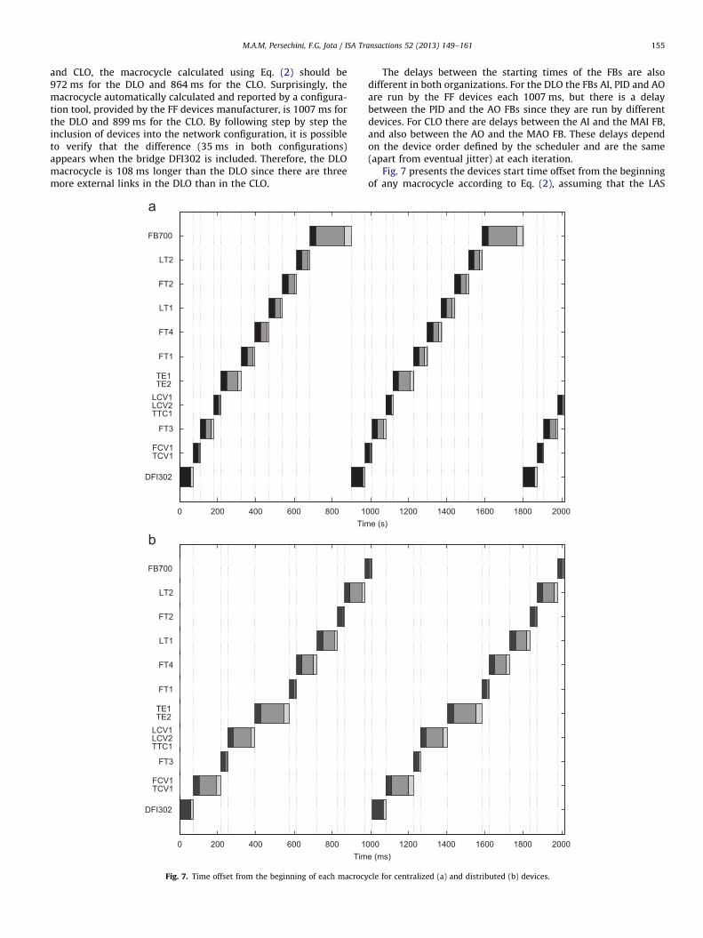
and CLO, the macrocycle calculated using Eq. (2) should be972 ms for the DLO and 864 ms for the CLO. Surprisingly, themacrocycle automatically calculated and reported by a configura-tion tool, provided by the FF devices manufacturer, is 1007 ms forthe DLO and 899 ms for the CLO. By following step by step theinclusion of devices into the network configuration, it is possibleto verify that the difference (35 ms in both configurations)appears when the bridge DFI302 is included. Therefore, the DLOmacrocycle is 108 ms longer than the DLO since there are threemore external links in the DLO than in the CLO.

0 200 400 600 800 1

DFI302

FT3

FT1

FT4

LT1

FT2

LT2

FB700

Tim

FCV1TCV1

LCV1LCV2TTC1

TE1TE2

0 200 400 600 800 1

DFI302

FT3

FT1

FT4

LT1

FT2

LT2

FB700

Tim

TE1TE2

LCV1LCV2TTC1

FCV1TCV1

Fig. 7. Time offset from the beginning of each macrocy

The delays between the starting times of the FBs are alsodifferent in both organizations. For the DLO the FBs AI, PID and AOare run by the FF devices each 1007 ms, but there is a delaybetween the PID and the AO FBs since they are run by differentdevices. For CLO there are delays between the AI and the MAI FB,and also between the AO and the MAO FB. These delays dependon the device order defined by the scheduler and are the same(apart from eventual jitter) at each iteration.

Fig. 7 presents the devices start time offset from the beginningof any macrocycle according to Eq. (2), assuming that the LAS

000 1200 1400 1600 1800 2000e (s)

000 1200 1400 1600 1800 2000e (ms)

cle for centralized (a) and distributed (b) devices.

M.A.M, Persechini, F.G, Jota / ISA Transactions 52 (2013) 149–161156

schedules the devices in ascending order of their addresses.In this figure, in which part (a) refers to the CLO and part (b) tothe DLO, black and grey marks indicate respectively the times forthe device to execute their FBs (30 ms) and to publish theirexternal links (30nNLE). The light grey mark corresponds to the20% extra time in Eq. (2). By analyzing Fig. 7(b), the delaysintroduced by the FF network in the TH level, TP level and TPoutput flowrate control loops are respectively 540 ms (from LT1at time 720 to LCV1 at time 1260), 396 ms (from LT2 at time 864to LCV2 at time 1260) and 468 ms (from FT4 at time 612 to FCV1at time 1080) for DLO.

Even though the CLO macrocycle is shorter than that of theDLO, the delays for the CLO depend not only on the device orderdefined by the scheduler in the FF network but also on thesynchronism between the function block scheduling in the FFnetwork and on the program that runs in the PLC. For the CLO theaverage scan time of the PLC program is 100.4 ms. Consideringonly the FF network scheduler, according to Fig. 7(a), the delaysbetween the AI and MAI FBs plus the ones between the MAO andAO FBs are 612 ms in the TH level control loop (from LT1 at time468 to LCV1 at time 1080), 468 ms in the TP level control loop(from LT2 at time 612 to LCV2 at time 1080), and 576 ms in the TPoutput flowrate control loop (from FT4 at time 396 to FCV1 attime 972). Besides, as there is no synchronization between thevalues published or subscribed by the FF network and the PLCscan, the delays between the MAI function block run by the FFnetwork and the PID run by the PLC can be up to one scan time,increasing the delay in each control loop. Therefore, the delaysintroduced by the FF network are greater for the CLO than for theDLO, and due to the lack of synchronism between the FBscheduler and the PLC program the control loops delays can varyup to one scan of an interaction to another for the CLO.

It is also important to consider the frequency with which thePID algorithm is run by the PLC program. Modern PLC models canrun interrupt service routines to ensure a constant period forcalling the PID controlling block, and this period can be defined bythe user. However, the PLC used in the control and automationarchitecture presented in this paper runs the PID block every scan.In consequence, as the FF network macrocycle is about eighttimes the PLC scan time, the PID block runs eight or nine timeswith the same process variable value, as verified experimentally.This repetition of the controlled variable value affect the PIDresults, especially the derivative term calculation. By analyzingEq. (1), it is verified that a low-pass filter with a time constantadjusted by the parameter a is added in the derivative term.However, the value of a is not configured by the user. In the caseof the PLC this value is not informed in its available documenta-tion, while a¼ 0:13 for the PID function block used by the FFnetwork and according to [24].

4. Controllers design

Taking Fig. 4 as reference, for control design purposes, the pilotplant is simply represented as a matrix of transfer functions in theLaplace domain such as

YLTPðsÞ

YLTHðsÞ

YFTPðsÞ

264

375¼

g11ðsÞ 0 g13ðsÞ g14ðsÞ

0 g22ðsÞ 0 g24ðsÞ

0 0 g33ðsÞ 0

264

375

ULTPðsÞ

ULTHðsÞ

UFTPðsÞ

UTTPðsÞ

266664

377775 ð3Þ

where

g11ðsÞ ¼0:106 e�4s

s; g13ðsÞ ¼

�0:195 e�4s

s

g14ðsÞ ¼0:030 e�4s

s; g22ðsÞ ¼

0:190 e�4s

s

g24ðsÞ ¼�0:035 e�4s

s; g33ðsÞ ¼

1:421 e�4s

sþ1ð4Þ

The transfer function parameter values in Eq. (4) have beendetermined from a set of different experiments, in which themanipulated variables, uLTP(t), uLTH(t), uFTP(t), and the disturbanceuTTP(t) were varied such that yLTP(t), yLTH(t) and yFTP(t) wereperturbed around their nominal operating range values. The timedelays seen in Eq. (4) include the delays introduced by the FFnetwork.

The PID parameters for the KLTP(s) and KLTH(s) controllers havebeen calculated using the technique presented in [25] namelyDirect Synthesis Design for Disturbance Rejection. In this case, tocalculate the TP level control loop, g13ðsÞ is considered thedisturbance model, g11ðsÞ is considered the process model andg14ðsÞ ¼ 0; and to calculate the TH level control loop, g24ðsÞ isconsidered the disturbance model and g22ðsÞ is considered theprocess model. Therefore, from Fig. 4, the closed-loop transferfunctions for disturbances is given by

YLTPðsÞ

UFTPðsÞ¼

g13ðsÞ

1þKLTPðsÞg11ðsÞð5Þ

and

YLTHðsÞ

UTTPðsÞ¼

g24ðsÞ

1þKLTHðsÞg22ðsÞð6Þ

By rearranging Eqs. (5) and (6) the controllers can be calculated as

KLTPðsÞ ¼g13ðsÞ

Y

D

� �ðsÞg11ðsÞ

�1

g11ðsÞð7Þ

and

KLTHðsÞ ¼g24ðsÞ

Y

D

� �ðsÞg22ðsÞ

�1

g22ðsÞð8Þ

where ðY=DÞðsÞ is the transfer function that represents the desiredclosed-loop response of the controlled variable, Y(s), when thedisturbance signal, D(s), occurs. Thus, the controlled and distur-bance variables are respectively YLTP(s) and UFTP(s), in Eq. (7), andYLTH(s) and UTTP(s), in Eq. (8). According to [25] when the processmodel and the disturbance model are described by an integratorplus time delay as given by g11ðsÞ, g22ðsÞ, g13ðsÞ and g24ðsÞ, and byrepresenting the time delay term by a first-order Pade approx-imation in Eqs. (7) and (8), the desired transfer function ðY=DÞðsÞ

needed to fit the controllers KLTP(s) and KLTH(s) into the PIDcontroller equation is specified as

Y

D

� �ðsÞ ¼

ðTi=KpÞsð1þy=2Þs

ðtcsþ1Þ3�

GpðsÞ

GdðsÞð9Þ

where Gp(s) is the process model, Gd(s) is the disturbance model andtc is a free user design parameter chosen to fit the desired closedloop disturbance rejection response of the controlled variable.

Substituting Eq. (9) into Eq. (7) and considering GpðsÞ ¼ g11ðsÞ

and GdðsÞ ¼ g13ðsÞ, and also substituting Eq. (9) into Eq. (8) andconsidering GpðsÞ ¼ g22ðsÞ and GdðsÞ ¼ g24ðsÞ, the resulting PIDparameters are

Kp ¼1

K

yð3tcþy=2Þ

ðtcþy=2Þ3; Ti ¼ 3tcþ

y2; Td ¼

ð3=2Þt2cyþð3=4Þtcy

2þy3=8�t3

c

yð3tcþy=2Þ:

ð10Þ

where K and y are respectively the gain and the time delay of theprocess models g11ðsÞ and g22ðsÞ.

The PID parameters for KFTP(s) have been calculated using theinternal model control approach as described in [26], where tc is

Table 1Controllers settings according to Eqs. (1), (10), (18) and (23).

Control settings TP level TH level TP flow

U(s) ULTP(s) ULTH(s) UFTP(s)

Y(s) YLTP(s) YLTH(s) YFTP(s)

Uff(s) UFTP(s) UTTP(s)

K 0.106 0.190 1.421

y 4 4 4

t 1

tc 7 7 10

Kp 1.19 0.66 0.17

Ti 23 23 3

Td 0.47 0.47 0.66

Kff 1.90 0.18

M.A.M, Persechini, F.G, Jota / ISA Transactions 52 (2013) 149–161 157

the desired closed loop time constant of the controlled variablewhen the set point changes, and K, y and t are respectively thegain, the time delay and the time constant of the process modelg33ðsÞ.

To use this approach, the time delay, y, is replaced by a firstorder Pade approximation, being the process model factored as

~g33ðsÞ ¼ ~g þ ðsÞ: ~g�ðsÞ ð11Þ

where

~g33ðsÞ ¼ K �1�

y2

s

1þy2

s

� �ðtsþ1Þ

ð12Þ

~g þ ðsÞ ¼ 1�y2

s ð13Þ

~g�ðsÞ ¼K

1þy2

s

� �ðtsþ1Þ

ð14Þ

The controller is specified as

KFTPðsÞ ¼GcðsÞ

1�GcðsÞ ~g33ðsÞð15Þ

where

GcðsÞ ¼1

~g�ðsÞf ðsÞ ð16Þ

and f(s) is a first order filter with unity gain and time constant tc

such as

f ðsÞ ¼1

tcsþ1ð17Þ

Substituting Eqs. (12), (14) and (17) into Eq. (15) and rearrangingthe coefficients into the PID controller equation (Eq. (1) with Kff ¼ 0and a¼ 0), the PID parameters are

Kp ¼1

K

2tyþ1

2tc

yþ1

; Ti ¼y2þt; Td ¼

t

2tyþ1

ð18Þ

The gain of the feedforward controllers K13 and K24 werecalculated based on dynamic models as described in [26]. Accord-ing to Fig. 4, the closed loop transfer function for load disturbanceinto TP and TH levels are respectively

YLTPðsÞ

UFTPðsÞ¼

g13ðsÞþK13g11ðsÞ

1þKLTPðsÞg11ðsÞð19Þ

and

YLTHðsÞ

UTTPðsÞ¼

g24ðsÞþK24g22ðsÞ

1þKLTHðsÞg22ðsÞð20Þ

The idea of the feedforward controller is to maintain thecontrolled variable exactly at the set point irrespective of changesin the disturbance variable. Therefore, considering the controlledvariables YLTPðsÞ ¼ 0 and YLTHðsÞ ¼ 0, and the disturbance variablesUFTPðsÞa0 and UTTPðsÞa0, we have

g13ðsÞþK13g11ðsÞ ¼ 0 ð21Þ

and

g24ðsÞþK24g22ðsÞ ¼ 0 ð22Þ

and the feedforward controllers are

K13 ¼�g13ðsÞ

g11ðsÞ; K24 ¼�

g24ðsÞ

g22ðsÞð23Þ

Table 1 summarizes the controller settings according toEqs. (1), (10), (18) and (23). The values of y, t, tc , Ti and Td aregiven in seconds.

5. Performance assessment of controllers

According to [27], one of the reasons for using control perfor-mance assessment (CPA) tools is to provide an online automatedprocedure that delivers information for determining whether thecontrolled variables are achieving the specified performance targets.A review of techniques used for CPA is presented in [27] andapplications of some of them are described, for example, in [28–31].

As far as CPA is concerned, a problem that still remains open isthe determination of which strategy, or control algorithm, is the bestfor a given application in comparison to others. Fair comparisonsbetween the behaviour of controllers can be done only if generalrules for control performance assessment are available. Dependingon the interest of the person that makes the evaluation, differentopinions about the same control behaviour could be made. So, inorder to get a comprehensive assessment of the behaviour of thesystem as a whole, a global index has to be defined.

Although performance assessment is viewed as a must by manyresearchers and practitioners, there seems to be no generallyacceptable metrics that could be applied in real operating condi-tions. Conventional indices, such as ISE and ITAE, do not givestraightforward indication of the actual control performance, sincethey vary according to operating conditions (set-point, disturbances,etc.) and even with the considered time window. Minimum varianceapproaches have been presented as an alternative but their resultsrely very much on the knowledge of the actual minimum or on theon-line estimation of the minimum variance (which is ratherunwieldy since it takes long time to converge). For this reasons,the authors decided to use an weighted control performanceassessment [32] capable of generating metrics according to threeassessors, namely, an engineer, an administrator and an user.A global index is then calculated as an weighted average of thethree metrics, all normalised in the range of 0–100.

5.1. Practical implementation of the performance indices

In [32], a global index, based on multiple criteria, particularlyappropriate for the assessment of performance of real industrialcontrol systems, is defined. The proposed method, besides thetime weighting feature in the index calculations, provides numer-ical conditioning in order to obtain adjustable sensitivity andselectivity. It also takes into account the actual control rangeavailable in any particular position of the final control elements.

The normalized indices, as detailed in the sequel, are calcu-lated by making use of various types of functions of the error andof the variances of the controlled and manipulated variables. Suchperformance indices are computed continuously, in real-time.

M.A.M, Persechini, F.G, Jota / ISA Transactions 52 (2013) 149–161158

One of the difficulties in implementing a continuous perfor-mance assessment, based on the absolute (or squared) error, isrelated to the unlimited growth of the integral as the timeincreases indefinitely. A possible way to solve this problem is touse of an exponential forgetting factor which yields an equivalentdata window, the so-called Asymptotic Sample Length, or ASL [33].Thus, a generic weighted index IN can be defined as

IN ¼

PNi ¼ 1 b

N�if ðiÞPNi ¼ 1 b

N�ið24Þ

where N is the total number of samples, b is the forgetting factor(0obr1) and f(i) is a function of a specific variable to beconsidered in the composition of the index of performance (oneof the functions shown in Table 2), calculated at the i-th samplinginstant. According to [32], b is a user-defined constant parameter,which is chosen a priori.

In order to give greater flexibility to the weighting procedure, ag factor can be introduced so that the index values are reinforced(or attenuated) in some ranges.

The various functions considered in this work for globalperformance assessment and their corresponding weightings arelisted in Table 2. Note that, for 0ogo1, the indices grow andthat, for g41, they are attenuated and, in the absence of extrainformation, g can be simply set to 1.

The Asymptotic Sample Length, defined as 1=ð1�bÞ, means thatthe last measurements are the ones that make greater contributionsto the current value of the computed index [33]. More precisely, theAsymptotic Sample Length corresponds to the number of samplesthat contributes to about 63% of the total value, irrespective of thetotal number of samples performed thus far.

The error and control signals are weighted differently for differentoperating conditions. Owing to the data weighting feature included inthe proposed scheme, the calculated values always lie in the range of[0,100]. The error, e(i), at sampling instant i, is normalised, as afunction of the actual control signal, in the following way:

en ¼

0 for 9eðiÞ9oE

100sateðiÞ

100�uðiÞ

� �for ½eðiÞZE

and ðuðiÞo100�

100sateðiÞ

uðiÞ

� �for ½eðiÞr�E

and uðiÞ40�

100 in any other case

8>>>>>>>>>>>>><>>>>>>>>>>>>>:

ð25Þ

Table 2Functions used in the composition of the indices of performance and their res-

pective acronyms.

Function Weighted index Acron.

9eðkÞ9g

Integral of the absolute error WIAE

eðkÞ2

100g2

Integral of the squared error WISE

k

g9eðkÞ9g

Integral of the time multiplied by absolute error WITAE

k

geðkÞ2

100g2

Integral of the time multiplied by the squared error WITSE

½uðkÞ�wðkÞ=g �2

100g2

Control signal variance WISU

9uðkÞ�u9gDumax

aControl signal activity WUA

9yðkÞ�y9gDymax

aOutput signal activity WYA

a Dxmax corresponds to the maximum possible variation of x in one sampling

interval.

where eðiÞ ¼ spðiÞ�yðiÞ, sp(i) and y(i) being respectively the values ofthe set-point and the output (controlled) variables at samplinginstant i; en represents the normalised error; u(i) is the control signalat time i; E defines a dead-zone which, in practice, is chosenaccording to the variance of the corresponding controlled variableand the function satf�g is given by

satfxg ¼

x for 9x9r1

9x9x

for 9x941

8><>: ð26Þ

The indices so defined and normalized as functions of the time,of the error and of the control and output signals, are taken intoaccount the users, the system manager and the control engineerto generate corresponding metrics (henceforward, referred hereas User Index, idU; Manager Index, idM; and Engineer Index, idE).They are used to express numerically the on-line performance of acontrol loop, producing a global performance index that can beused in the choice of the best control strategy or even in thetuning of the controller parameters or deciding on whether thecontrol system is faulty or not.

The method has also a great potential of application in the areaof quality control in production lines. These three people oftenmake use of guidelines that could be objective or subjective; inthe first case the human opinion is not considered and, in thelatter, statistical measurements or other forms of quantifyingsubjective opinion are used [32].

The global index idG, as an overall assessment of the controlsystem, should reflect the actual performance of the system andgive grades reasonably acceptable by the three assessors. Moredetails on how the four indices (idU, idE, idM and idG) arecalculated can be found in [32]. As each one of these indices isweighted and constrained to a range between 0 and 100, theperformance values also lie between 0 and 100.

6. Experimental results

Preliminary experiments have been performed in the pilotplant and analysed for both centralized and distributed organiza-tions; as a consequence, some of PID parameter settings wereslightly modified to improve the controllers’ performance: theproportional gain of KLTH(s) was changed from 0.66 to 0.90 andthe integral time of KFTP(s) was changed from 3.0 s to 4.5 s.

After these adjustments, typical results for the TH level, TPlevel and TP flowrate control loops are shown in Fig. 8, in whichthe results of the experiment performed in DLO are representedby solid lines, while those performed in CLO are represented indotted lines.

The data points show in Fig. 8 were sampled at the same time andwere grouped by control loop. For the TH level control loop,Fig. 8(a) shows the set point spLTH(t) and the controlled variableyLTH(t)), Fig. 8(b) shows the manipulated variable uLTH(t) that is thesignal sent to the control valve LCV1, and Fig. 8(c) shows the globalperformance index idGLTH(t). For the TP level control loop, Fig. 8(d)shows the set point spLTP(t) and the controlled variable yLTP(t)),Fig. 8(e) shows the manipulated variable uLTP(t) that is the signalsent to the control valve LCV2, and Fig. 8(f) shows the globalperformance index idGLTP(t). For the TP output flowrate control loop,Fig. 8(g) shows the set point spFTP(t) and the controlled variableyFTP(t)), Fig. 8(h) shows the manipulated variable uFTP(t) that is thesignal sent to the control valve FCV1, and Fig. 8(i) shows the globalperformance index idGFTP(t). The set points of the three controlledvariables were changed during the experiment shown in Fig. 8.The TH level set point spLTH(t) was changed from 200 mm to 300 mmat time t¼330 s and returned to 200 mm at time t¼2700 s (Fig. 8(a)).The TP level set point spLTP(t) was changed from 300 mm to 400 mm

0 500 1000 1500 2000 2500 3000150200250300350

y LTH

(mm

)

0 500 1000 1500 2000 2500 30000

1020304050

u LTH

(%)

0 500 1000 1500 2000 2500 30005060708090

100

idG

LTH (%

)

0 500 1000 1500 2000 2500 3000250300350400450

y LTP

(mm

)

0 500 1000 1500 2000 2500 30000

204060

u LTP

(%)

0 500 1000 1500 2000 2500 300040

60

80

100

idG

LTP (%

)

0 500 1000 1500 2000 2500 3000

202530

y FTP

(l/m

)

0 500 1000 1500 2000 2500 30003032343638

u FTP

(%)

0 500 1000 1500 2000 2500 300080859095

100

idG

FTP (%

)

Time (s)

Fig. 8. Typical experimental results where the solid lines represent the experi-

ment in the distributed logical organization, and dotted lines the experiment in

the centralized logical organization.

M.A.M, Persechini, F.G, Jota / ISA Transactions 52 (2013) 149–161 159

at time t¼930 s and returned to 300 mm at time t¼2700 s(Fig. 8(d)). The TP output flowrate set point spFTP(t) was changedfrom 20 l/m to 30 l/m at time t¼2130 s and returned to 20 l/m attime t¼2700 s (Fig. 8(g)).

It is worth mentioning that uTTP(t), the signal sent to thecontrol valve TCV1 installed between TH and TP was manipulatedduring the experiment by setting it to 40% at time t¼0 s, to 25% attime t¼1500 s and again to 40% at time t¼2700 s.

By analysing Fig. 8, it can be seen that the same sequence of setpoints was applied to both logical organizations, and that, whencomparing DLO with CLO (solid lines and dotted lines respec-tively) in each one of the three control loops, the behaviour of thecontrolled variables (Fig. 8(a), (d), and (g)) and manipulatedvariables (Fig. 8(b), (e) and (h)) is very similar, notably for theTP and TH levels. In addition, the global indices idG, althoughshowing the same trend, have different values for the DLO andCLO configurations for the TH level control loop (Fig. 8(c)), thevalues of idGLTH(t) from the set point change at time t¼930 s up tothe end of the experiment are greater for DLO than for CLO; forthe TP level control loop (Fig. 8 (f)), the values of idGLTP(t) aregreater for DLO than for CLO during all the experiment; and forthe TP flowrate control loop (Fig. 8 (i)), the values of idGFTP(t) aregreater for DLO than for CLO at the beginning of the experiment,between t¼0 s and t¼440 s, and at the end of experiment,between t¼2280 s and t¼3330 s. Table 3 presents the final valuesof the control performance assessment indices at time t¼3300 s.

A closer examination of the performance indices for the threecontrol loops (Table 3) reveals that their values are greater forDLO if compared to the CLO ones. For example, idGLTH is equal to55.52% for DLO and equal to 53.85% for CLO, for the TH levelcontrol loop; idGLTP is equal to 66.13% for DLO and equal to 63.55%for CLO, for the TP level control loop; and idGFTP is equal to 85.62%for DLO and equal to 85.21% for CLO, for the TP flowrate controlloop. The differences are respectively 1.67%, 2.58% and 0.41% forthe TH level, TP level and TP flowrate control loops. Althoughthese differences are small, their values are significant when onetakes into account the maximum idG index reached for eachcontrol loop; for example, the maximum global index is respec-tively 85.42%, 96.78% and 97.07% for the TH level, TP level and TPflowrate control loops. Moreover, the differences remain roughlythe same for the TP and TH level control loops throughout theexperiment.

Therefore, the results shown in Fig. 8 and Table 3 indicate that,during most of the time, the control loops that had been config-ured in a distributed logical organization reached performanceindices greater than the control loops configured in a centralizedlogical organization. Other experiments were performed by usingthe same control strategy with different parameters of the PIDcontrollers, and also by modifying the control strategy by remov-ing the feedforward controllers. In all these cases the resultsindicated that DLO reached performance indices greater than thecontrol loops configured in a CLO.

As stated in Section 3.3, differences on the FF networkscheduling and on the synchronization of the functions formeasuring the controlled variables, calculating the PID algorithmand sending the output signal to the manipulated variables couldexplain the performance differences between both logical orga-nizations. Since there are no time synchronism between thefunction blocks scheduling in the FF network and the programthat runs in the PLC, this could cause variations on the delaysintroduced by the FF network in each iteration, reducing theperformance of the CLO. Moreover, an incorrect setting ofthe low-pass filter time constant could cause oscillations in themanipulated variable calculated by the CLO.

Another aspect to be considered is the relationship betweenthe delay introduced by the FF network and the control loop

Table 3Values of the control performance assessment indices at the end of the experiment.

TH level

Distributed Centralized

idELTH idMLTH idULTH idGLTH idELTH idMLTH idULTH idGLTH

55.39 74.20 36.97 55.52 53.54 73.17 34.85 53.85

TP level

Distributed Centralized

idELTP idMLTP idULTP idGLTP idELTP idMLTP idULTP idGLTP

65.47 78.24 54.69 66.13 62.81 76.92 50.93 63.55

TP flow

Distributed Centralized

idEFTP idMFTP idUFTP idGFTP idEFTP idMFTP idUFTP idGFTP

85.72 91.19 79.95 85.62 85.36 90.96 79.31 85.21

M.A.M, Persechini, F.G, Jota / ISA Transactions 52 (2013) 149–161160

dynamic. In this case, the delay introduced by the network isapproximately 0.5 s in both logical configurations, and as shown inTable 1, the control loop design considers a time delay equal to 4 sand a time constant equal to respectively 7 s, 7 s and 10 s for the THlevel, TP level and TP flowrate control loops. Also, the differencebetween the delays introduced in each control loop by the networkcomputed for CLO and for DLO is less than 0.1 s. Therefore, thedelays introduced by the network add a very small contribution tothe control loop dynamics. The relevant fact that could be related tothe small difference in the control performance assessment indicesbetween one configuration and another is the lack of synchronismbetween the FF network scheduler and the PLC program in thecentralized logical organization.

7. Conclusions

An experimental setup using commercial devices and a Founda-tion Fieldbus network has been used to implement the controlstrategies in both centralized and distributed logical organizations.Despite the fact that manufacturers do not make available details oftheir software implementation, an analysis of the fieldbus networkscheduling was made for the considering configurations. It indicatedthat the delays introduced by the network are around 500 ms.Moreover, the delays in the centralized configuration are larger thanin the distributed one although the macrocycle calculated for thelatter is 108 ms greater for centralized configuration.

The design of the control system has been defined taking intoaccount not only the dynamics of the process, but also thecharacteristics and limitations of the available architecture, particu-larly, the requirement of using of PID controllers with a feedforwordaction. This resulted in a simple and an efficient controller design,with acceptable performance in both logical organizations.

The control performance assessment indices provided aninsight that could not be achieved by simple visual inspection ofthe time series profiles of both controlled and manipulatedvariables. These indices have more precisely pointed out whereand for how much one configuration is better than the other.The assessment revealed that the overall control performance wasslightly better in the distributed organization. The final indiceshave indicated an improvement between 0.4% and 2.5% in allcontrol loops. These differences can be explained by the way thedelays occur in the network environment and by the lack of

synchronism in the centralized logical organization between thefunction block scheduling in the Foundation Fieldbus networkand the program that runs in the PLC.

To improve the performance of the centralized organization, itwould be necessary to implement some form of synchronismbetween the program that runs in the PLC and the networkscheduling. These results emphasize the importance of consider-ing not only the physical allocation of the available resources butalso the consequences of their logical distribution on the feedbackcontrol system.

References

[1] Samad T, McLaughlin P, Lu J. System architecture for process automation:review and trends. Journal of Process Control 2007;17:191–201.

[2] ANSI/ISA-95.00.03, Enterprise control system integration part 3: activitymodels of manufacturing operations management; 2005.

[3] Neumann P. Communication in industrial automation. What is going on?Control Engineering Practice 2007;15:1332–47.

[4] Thomesse J-P. Fieldbus technology in industrial automation. Proceedings ofthe IEEE 2005;93(6):1073–101.

[5] Sirkka-Liisa, Jamsa-Jounela, Future trends in process automation, AnnualReviews in Control 31 (2007) 211–20.

[6] Gupta RA, Chow M-Y. Networked control system: overview and researchtrends. IEEE Transactions on Industrial Electronics 2010;57(7):2527–35.

[7] Hespanha JP, Naghshtabrizi P, Xu Y. A survey of recent results in networkedcontrol systems. Proceedings of the IEEE 2007;95(1):138–62.

[8] Baillieul J, Antsaklis PJ. Control and communication challenges in networkedreal-time systems. Proceedings of the IEEE 2007;95(1):9–28.

[9] Fadaei A, Asgarian E, Salahshoor K. Function block and networked controlsystem implementation on a real pilot plant. In: IEEE international confer-ence on industrial technology; 2008.

[10] Karami J, Salahshoor K. Design and implementation of an instructionalfoundation fieldbus-based pilot plant. In: International multi-conference oncomputing in the global information technology; 2006.

[11] Mohammadove G, Salahshoor K. Design and implementation of an instruc-tional foundation fieldbus-based pilot plant (operation phase). In: IEEEChinese control conference; 2006.

[12] Ahdel-Ghaffar HF, Abdel-Magied MF, Fikri M, Kame M. Performance analysisof fieldbus in process control systems. In: IEEE proceedings of the Americancontrol conference. Colorado: Denver; 2003.

[13] Li Q, Rankin DJ, Jiang J. Evaluation of delays induced by foundation fieldbusH1 networks. IEEE Transactions on Instrumentation and Measurement2009;58(10):3584–692.

[14] Pang Y, Yang S-H, Nishitanic H. Analysis of control interval for foundationfieldbus-based control. ISA Transactions 2006;45:458–77.

[15] Lee YH, Hong SH. Dependency on prioritized data in the delay analysis offoundation fieldbus. Control Engineering Practice 2010;18:845–51.

[16] Hong SH, Song SM. Transmission of a scheduled message using a foundationfieldbus protocol. IEEE Transactions on Instrumentation and Measurement2008;57(2):268–75.

M.A.M, Persechini, F.G, Jota / ISA Transactions 52 (2013) 149–161 161

[17] Z. Xiang-li, Study on communication scheduling of fieldbus. In: IEEE Chinesecontrol and decision conference; 2009. p. 565–70.

[18] Fadaei A, Salahshoor K. Design and implementation of a new fuzzy PIDcontroller for networked control systems. ISA Transactions 2008;47:351–61.

[19] Machado V, Neto ADD, de Melo JD. A neural network multiagent architectureapplied to industrial networks for dynamic allocation of control strategiesusing standard function blocks. IEEE Transactions on Industrial Electronics2010;57(5):1823–34.

[20] Geng L, Yan B. Application of foundation fieldbus technology in chain grateboiler automation control system. In: The eighth international conference onelectronic measurement and instruments; 2007.

[21] Smar; July 2010 /www.smar.comS.[22] J. Berge, Introduction to fieldbuses for process control. In: Fieldbuses for

process control: engineering, operation, and maintenance. ISA; 2002. p. 1–26.[23] Smar Co., DFI302 – user manual of fieldbus universal bridge; 2002.[24] Smar Co., Library A: function blocks instruction manual; February 2008.[25] Chen D, Seborg DE. PI/PID controller design based on direct synthesis and

disturbance rejection. Industrial and Engineering Chemistry Research 2002;41:4807–22.

[26] Seborg DE, Edgar TF, Mellichamp DA. Process dynamics and control.John Wiley & Sons; 1989.

[27] Jelali M. An overview of control performance assessment technology and

industrial applications. Control Engineering Practice 2006;14:441–66.[28] Ko B-S, Edgar TF. PID control performance assessment: the single-loop case.

AIChE Journal 2004;50(6):1211–8.[29] Lee KH, Tamayo EC, Huang B. Industrial implementation of controller

performance analysis technology. Control Engineering Practice 2010;18:147–58.

[30] Ingimundarson A, Hagglund T. Closed-loop performance monitoring usingloop tuning. Journal of Process Control 2005;15:127–33.

[31] Veronesi M, Visioli A. Performance assessment and retuning of PID con-trollers for integral processes. Journal of Process Control 2010;20:261–9.

[32] Jota FG, Braga AR, Pena RT. Performance assessment of advanced processcontrol algorithms using an interacting tank system. In: Conference recordsof the 30th annual meeting of the IEEE-IAS, vol. 2; 1995. p. 1565–71 .

[33] Clarke DW. self-tuning control. The control handbook. IEEE Press; 1996.p. 827–46.