Central Bank Swap Lines

Saleem BahajBank of England

Ricardo ReisLSE

ECB - Global Research Forum

29th of November, 2018

The views expressed are those of the presenters and not necessarily those of the Bank of England, the MPC, the FPC or the PRC.

CB swap lines post 2007

The governor of the Reserve Bank of India on Sunday called on major central banks to extend their network of currency swap lines deep into emerging markets, saying a type of “virtual apartheid” in the provision of foreign currencies hampers efforts to fight financial instability.” Wall Street Journal, October 15, 2017.

Source: Denbeem, Jung, Paterno (2016)

This paper1. How do swap lines work and what is their role in monetary policy? • Source country CB lending to recipient country banks. Recipient CB bears credit risk/

monitors.

2. How does this monetary policy transmit through financial markets?• Ceiling on CIP deviations => lower funding costs

3. What economic consequences does this have? 1. Encourage investment from recipient- country banks into assets denominated in the source-

country’s currency.2. Increases the expected profits of recipient-country banks that invest in source country.

Empirics: difference-in-differences strategy around the change in Fed Swap Line Rate in November 2011. Models: Not going to go into details today.

1. Role in central banking: how the swap lines work

ECB borrowing USD from Fed1. Fed sells dollars to ECB, ECB sells euros back at today’s spot exchange rate. 2. Agree in one week to resell, so euros are collateral.3. Settlement happens at the same exchange rate.4. Fed charges an interest rate in dollars set at start ($ OIS+spread).5. ECB lends to EA bank, charges same rate, collect HQLA as collateral,

determines who is eligible.6. ECB in charge of collecting payment.

Liquidity assistance to foreign bank using foreign central bank to do the monitoring of collateral and bank.

Functions and alternativesProperties• US monetary policy on monetary base and rate, not EA monetary policy• No exchange-rate or interest-rate risk, ECB has credit risk as in any lending facility

Basic function of central banks:• Fed: provide liquidity when there is a funding crisis• ECB: judge banks eligible for liquidity assistance• Not exchange-rate pegs, not IMF loans, not US bailout of foreign banks

Alternatives (beyond FX reserves):1. Fed lends directly to EZ banks through discount window/TAF? But (i) less efficient

monitoring, Fed refuse, (ii) branches/subsidiaries did not have collateral; (iii) stigma. 2. EZ banks borrow euros from ECB buy dollars, swap out the currency risk? Spot and

forward markets never closed, but cost…

2. Financial market effects of swap lines

Theory• Trade involving only a bank and the central bank (all in logs)• EZ bank borrows dollars for one week from ECB swap line, pay is • Buys euros at spot rate s, and sell forward at rate f in one week • Deposit euros at ECB at at rate iv* • Swap overnight for one-week rate at cost i*-ip*

• Deviations from CIP:

• Proposition: Deviations from covered interest parity have a ceiling given by the spread between the source swap and interbank rates plus the difference between the recipient central bank policy and deposit rates:

ist � st � ft + (iv⇤t + i⇤t � ip⇤t )<latexit sha1_base64="GP2Anj4jIFo3m5tHFJ5l7GRSH2M=">AAACLXicdVDLSgMxFM34tr6qLt0Ei+ADSyJi252gC5cKVoW2Dpk0U0MzD5I7Qhnmh9z4KyK4UMStv2FSK6johZBzzzmX5J4gVdIAIc/e2PjE5NT0zGxpbn5hcam8vHJhkkxz0eSJSvRVwIxQMhZNkKDEVaoFiwIlLoP+kdMvb4U2MonPYZCKTsR6sQwlZ2Apv3ws/RyK69wUuN0T2LgO7+JweO/gzZF8u+066cN1mxmwBgfz1DUF3vLLFVIlhFBKsQO0dkAsaDTqe7SOqZNsVdCoTv3yY7ub8CwSMXDFjGlRkkInZxokV6IotTMjUsb7rCdaFsYsEqaTD7ct8IZlujhMtD0x4CH7fSJnkTGDKLDOiMGN+a058i+tlUFY7+QyTjMQMf98KMwUhgS76HBXasFBDSxgXEv7V8xvmGYcbMAlG8LXpvh/cLFXpaRKz/YrhyejOGbQGlpHm4iiGjpEJ+gUNRFHd+gBPaMX79578l69t0/rmDeaWUU/ynv/AFR/p5I=</latexit><latexit sha1_base64="GP2Anj4jIFo3m5tHFJ5l7GRSH2M=">AAACLXicdVDLSgMxFM34tr6qLt0Ei+ADSyJi252gC5cKVoW2Dpk0U0MzD5I7Qhnmh9z4KyK4UMStv2FSK6johZBzzzmX5J4gVdIAIc/e2PjE5NT0zGxpbn5hcam8vHJhkkxz0eSJSvRVwIxQMhZNkKDEVaoFiwIlLoP+kdMvb4U2MonPYZCKTsR6sQwlZ2Apv3ws/RyK69wUuN0T2LgO7+JweO/gzZF8u+066cN1mxmwBgfz1DUF3vLLFVIlhFBKsQO0dkAsaDTqe7SOqZNsVdCoTv3yY7ub8CwSMXDFjGlRkkInZxokV6IotTMjUsb7rCdaFsYsEqaTD7ct8IZlujhMtD0x4CH7fSJnkTGDKLDOiMGN+a058i+tlUFY7+QyTjMQMf98KMwUhgS76HBXasFBDSxgXEv7V8xvmGYcbMAlG8LXpvh/cLFXpaRKz/YrhyejOGbQGlpHm4iiGjpEJ+gUNRFHd+gBPaMX79578l69t0/rmDeaWUU/ynv/AFR/p5I=</latexit><latexit sha1_base64="GP2Anj4jIFo3m5tHFJ5l7GRSH2M=">AAACLXicdVDLSgMxFM34tr6qLt0Ei+ADSyJi252gC5cKVoW2Dpk0U0MzD5I7Qhnmh9z4KyK4UMStv2FSK6johZBzzzmX5J4gVdIAIc/e2PjE5NT0zGxpbn5hcam8vHJhkkxz0eSJSvRVwIxQMhZNkKDEVaoFiwIlLoP+kdMvb4U2MonPYZCKTsR6sQwlZ2Apv3ws/RyK69wUuN0T2LgO7+JweO/gzZF8u+066cN1mxmwBgfz1DUF3vLLFVIlhFBKsQO0dkAsaDTqe7SOqZNsVdCoTv3yY7ub8CwSMXDFjGlRkkInZxokV6IotTMjUsb7rCdaFsYsEqaTD7ct8IZlujhMtD0x4CH7fSJnkTGDKLDOiMGN+a058i+tlUFY7+QyTjMQMf98KMwUhgS76HBXasFBDSxgXEv7V8xvmGYcbMAlG8LXpvh/cLFXpaRKz/YrhyejOGbQGlpHm4iiGjpEJ+gUNRFHd+gBPaMX79578l69t0/rmDeaWUU/ynv/AFR/p5I=</latexit><latexit sha1_base64="GP2Anj4jIFo3m5tHFJ5l7GRSH2M=">AAACLXicdVDLSgMxFM34tr6qLt0Ei+ADSyJi252gC5cKVoW2Dpk0U0MzD5I7Qhnmh9z4KyK4UMStv2FSK6johZBzzzmX5J4gVdIAIc/e2PjE5NT0zGxpbn5hcam8vHJhkkxz0eSJSvRVwIxQMhZNkKDEVaoFiwIlLoP+kdMvb4U2MonPYZCKTsR6sQwlZ2Apv3ws/RyK69wUuN0T2LgO7+JweO/gzZF8u+066cN1mxmwBgfz1DUF3vLLFVIlhFBKsQO0dkAsaDTqe7SOqZNsVdCoTv3yY7ub8CwSMXDFjGlRkkInZxokV6IotTMjUsb7rCdaFsYsEqaTD7ct8IZlujhMtD0x4CH7fSJnkTGDKLDOiMGN+a058i+tlUFY7+QyTjMQMf98KMwUhgS76HBXasFBDSxgXEv7V8xvmGYcbMAlG8LXpvh/cLFXpaRKz/YrhyejOGbQGlpHm4iiGjpEJ+gUNRFHd+gBPaMX79578l69t0/rmDeaWUU/ynv/AFR/p5I=</latexit>

xt (ist � it) + (ip⇤t � i

v⇤t )

<latexit sha1_base64="rLq16oBSNlfnPMeHe6Pg7Lu8zho=">AAACl3icdVHbahsxENVub+n25qZ9KX0Zagx2g40USuIUSgMpJY8J1EnA6yxaWeuIaC9I2lCz7C/1Y/rWv6mkbKlb2gGhM3POYUajtJJCG4x/BOGdu/fuP9h6GD16/OTps97z7TNd1orxGStlqS5SqrkUBZ8ZYSS/qBSneSr5eXp95PjzG660KIsvZl3xRU5XhcgEo8aWkt63gUga0142uoV4xUG7DMaQ+XsHhh1989ZlIjGXMdXGChxsKpe0MIoG0eCrE37w/rF373RWrxn7xOq8DGLJYQi/W49vMYw2WlYbRj/AKIqSXh9PMMaEEHCA7O9hCw4OprtkCsRRNvqoi5Ok9z1elqzOeWGYpFrPCa7MoqHKCCZ5G8W15hVl13TF5xYWNOd60fi9tjCwlSVkpbKnMOCrm46G5lqv89Qqc2qu9N+cK/6Lm9cmmy4aUVS14QW7bZTVEkwJ7pNgKRRnRq4toEwJOyuwK6ooM/Yr3RJ+vRT+D852JwRPyOm7/uFxt44t9Bq9QUNE0D46RMfoBM0QC14G74Oj4FP4KvwYfg47bRh0nhfojwhPfwLAA8f1</latexit><latexit sha1_base64="rLq16oBSNlfnPMeHe6Pg7Lu8zho=">AAACl3icdVHbahsxENVub+n25qZ9KX0Zagx2g40USuIUSgMpJY8J1EnA6yxaWeuIaC9I2lCz7C/1Y/rWv6mkbKlb2gGhM3POYUajtJJCG4x/BOGdu/fuP9h6GD16/OTps97z7TNd1orxGStlqS5SqrkUBZ8ZYSS/qBSneSr5eXp95PjzG660KIsvZl3xRU5XhcgEo8aWkt63gUga0142uoV4xUG7DMaQ+XsHhh1989ZlIjGXMdXGChxsKpe0MIoG0eCrE37w/rF373RWrxn7xOq8DGLJYQi/W49vMYw2WlYbRj/AKIqSXh9PMMaEEHCA7O9hCw4OprtkCsRRNvqoi5Ok9z1elqzOeWGYpFrPCa7MoqHKCCZ5G8W15hVl13TF5xYWNOd60fi9tjCwlSVkpbKnMOCrm46G5lqv89Qqc2qu9N+cK/6Lm9cmmy4aUVS14QW7bZTVEkwJ7pNgKRRnRq4toEwJOyuwK6ooM/Yr3RJ+vRT+D852JwRPyOm7/uFxt44t9Bq9QUNE0D46RMfoBM0QC14G74Oj4FP4KvwYfg47bRh0nhfojwhPfwLAA8f1</latexit><latexit sha1_base64="rLq16oBSNlfnPMeHe6Pg7Lu8zho=">AAACl3icdVHbahsxENVub+n25qZ9KX0Zagx2g40USuIUSgMpJY8J1EnA6yxaWeuIaC9I2lCz7C/1Y/rWv6mkbKlb2gGhM3POYUajtJJCG4x/BOGdu/fuP9h6GD16/OTps97z7TNd1orxGStlqS5SqrkUBZ8ZYSS/qBSneSr5eXp95PjzG660KIsvZl3xRU5XhcgEo8aWkt63gUga0142uoV4xUG7DMaQ+XsHhh1989ZlIjGXMdXGChxsKpe0MIoG0eCrE37w/rF373RWrxn7xOq8DGLJYQi/W49vMYw2WlYbRj/AKIqSXh9PMMaEEHCA7O9hCw4OprtkCsRRNvqoi5Ok9z1elqzOeWGYpFrPCa7MoqHKCCZ5G8W15hVl13TF5xYWNOd60fi9tjCwlSVkpbKnMOCrm46G5lqv89Qqc2qu9N+cK/6Lm9cmmy4aUVS14QW7bZTVEkwJ7pNgKRRnRq4toEwJOyuwK6ooM/Yr3RJ+vRT+D852JwRPyOm7/uFxt44t9Bq9QUNE0D46RMfoBM0QC14G74Oj4FP4KvwYfg47bRh0nhfojwhPfwLAA8f1</latexit><latexit sha1_base64="rLq16oBSNlfnPMeHe6Pg7Lu8zho=">AAACl3icdVHbahsxENVub+n25qZ9KX0Zagx2g40USuIUSgMpJY8J1EnA6yxaWeuIaC9I2lCz7C/1Y/rWv6mkbKlb2gGhM3POYUajtJJCG4x/BOGdu/fuP9h6GD16/OTps97z7TNd1orxGStlqS5SqrkUBZ8ZYSS/qBSneSr5eXp95PjzG660KIsvZl3xRU5XhcgEo8aWkt63gUga0142uoV4xUG7DMaQ+XsHhh1989ZlIjGXMdXGChxsKpe0MIoG0eCrE37w/rF373RWrxn7xOq8DGLJYQi/W49vMYw2WlYbRj/AKIqSXh9PMMaEEHCA7O9hCw4OprtkCsRRNvqoi5Ok9z1elqzOeWGYpFrPCa7MoqHKCCZ5G8W15hVl13TF5xYWNOd60fi9tjCwlSVkpbKnMOCrm46G5lqv89Qqc2qu9N+cK/6Lm9cmmy4aUVS14QW7bZTVEkwJ7pNgKRRnRq4toEwJOyuwK6ooM/Yr3RJ+vRT+D852JwRPyOm7/uFxt44t9Bq9QUNE0D46RMfoBM0QC14G74Oj4FP4KvwYfg47bRh0nhfojwhPfwLAA8f1</latexit>

Further discussion: haircuts and regulationProposition: Bank-specific deviations from covered interest parity have a ceiling given by the spread between the source swap and interbank rates, plus the difference between the recipient central bank policy and deposit rates, plus the shadow value of collateral, plus the shadow cost of regulation on banks that is triggered by borrowing and lending from their central bank:

•Two independent sources of policy variation, domestic and foreign• Safe bank or sovereign fund: minimum.•Clear measure of CIP is the OIS one.

xa,t (ist � it) + (ip⇤t � i

v⇤t ) + (1� ⇠

c)(iua,t � i

st ) + a,t.

<latexit sha1_base64="YyLZDIDE/4iWPJGBBIZHgbXtN+E=">AAAFIHicpVRLb9NAEHabACW8WjhyGVFFimkT2SFKyiFSxUs9Fok+pDix1ptJstQvvOuqqeWfwoW/woUDCMENfg2766QN0PbSlSzPfjPfzDfjXXuxz7iwrF9Ly6XyjZu3Vm5X7ty9d//B6trDfR6lCcU9GvlRcugRjj4LcU8w4eNhnCAJPB8PvKOXyn9wjAlnUfhOTGPsB2QcshGjREjIXSu1qy/8FD1MkinodJvA2SlCa6tSZW4m8kHGc3DGCFztoA4j/d6A2sx9/FTtmCsGDuFCBigzi9UmB7NSrVRPVGBX8+uavTGj6pi63pzFgeMj1OC8dr2wwVyoGS8wtQLzunzltOvOCTN10PtN3SsbcFcon3OKghSw01e1ZJMKfoW+IAN0xX9YWmAnEpOJrihcBycNh5h4CaGYQQ+ChbSFrMA8E3eePXczBz+k7BgmtYapBwhyAkQp717dqTNUSVwCk3mFOWJePDqd/M1Frg24rBCYXVvznICIiedlr3OX1GYKze6lNCnPI0lWKMon+rwohQugWTsTUjCVwHnv1/z+A6pOgBxwkW3xDMScFWij4q6uW43nW+1mqw1Ww7I6dtNWRrPTetYCWyJqrRuzteuu/nSGEU0DDAX1Cec924pFPyOJYNTHvOKkHGNCj8gYe9IMSYC8n+kbmUNVIkMYRYl8QlHc00VGRgLOp4EnI9Ws+b8+BV7k66VitNXPWBinAkNaFBqlPogI1N8ChixBKvypNAhNmNQKdELkQRXyn6KGMO8ULjf2mw3bathvW+vbO7NxrBiPjSdGzbCNjrFt7Bi7xp5BSx9Ln0tfS9/Kn8pfyt/LP4rQ5aUZ55Hx1yr//gMCM6T3</latexit><latexit sha1_base64="YyLZDIDE/4iWPJGBBIZHgbXtN+E=">AAAFIHicpVRLb9NAEHabACW8WjhyGVFFimkT2SFKyiFSxUs9Fok+pDix1ptJstQvvOuqqeWfwoW/woUDCMENfg2766QN0PbSlSzPfjPfzDfjXXuxz7iwrF9Ly6XyjZu3Vm5X7ty9d//B6trDfR6lCcU9GvlRcugRjj4LcU8w4eNhnCAJPB8PvKOXyn9wjAlnUfhOTGPsB2QcshGjREjIXSu1qy/8FD1MkinodJvA2SlCa6tSZW4m8kHGc3DGCFztoA4j/d6A2sx9/FTtmCsGDuFCBigzi9UmB7NSrVRPVGBX8+uavTGj6pi63pzFgeMj1OC8dr2wwVyoGS8wtQLzunzltOvOCTN10PtN3SsbcFcon3OKghSw01e1ZJMKfoW+IAN0xX9YWmAnEpOJrihcBycNh5h4CaGYQQ+ChbSFrMA8E3eePXczBz+k7BgmtYapBwhyAkQp717dqTNUSVwCk3mFOWJePDqd/M1Frg24rBCYXVvznICIiedlr3OX1GYKze6lNCnPI0lWKMon+rwohQugWTsTUjCVwHnv1/z+A6pOgBxwkW3xDMScFWij4q6uW43nW+1mqw1Ww7I6dtNWRrPTetYCWyJqrRuzteuu/nSGEU0DDAX1Cec924pFPyOJYNTHvOKkHGNCj8gYe9IMSYC8n+kbmUNVIkMYRYl8QlHc00VGRgLOp4EnI9Ws+b8+BV7k66VitNXPWBinAkNaFBqlPogI1N8ChixBKvypNAhNmNQKdELkQRXyn6KGMO8ULjf2mw3bathvW+vbO7NxrBiPjSdGzbCNjrFt7Bi7xp5BSx9Ln0tfS9/Kn8pfyt/LP4rQ5aUZ55Hx1yr//gMCM6T3</latexit><latexit sha1_base64="YyLZDIDE/4iWPJGBBIZHgbXtN+E=">AAAFIHicpVRLb9NAEHabACW8WjhyGVFFimkT2SFKyiFSxUs9Fok+pDix1ptJstQvvOuqqeWfwoW/woUDCMENfg2766QN0PbSlSzPfjPfzDfjXXuxz7iwrF9Ly6XyjZu3Vm5X7ty9d//B6trDfR6lCcU9GvlRcugRjj4LcU8w4eNhnCAJPB8PvKOXyn9wjAlnUfhOTGPsB2QcshGjREjIXSu1qy/8FD1MkinodJvA2SlCa6tSZW4m8kHGc3DGCFztoA4j/d6A2sx9/FTtmCsGDuFCBigzi9UmB7NSrVRPVGBX8+uavTGj6pi63pzFgeMj1OC8dr2wwVyoGS8wtQLzunzltOvOCTN10PtN3SsbcFcon3OKghSw01e1ZJMKfoW+IAN0xX9YWmAnEpOJrihcBycNh5h4CaGYQQ+ChbSFrMA8E3eePXczBz+k7BgmtYapBwhyAkQp717dqTNUSVwCk3mFOWJePDqd/M1Frg24rBCYXVvznICIiedlr3OX1GYKze6lNCnPI0lWKMon+rwohQugWTsTUjCVwHnv1/z+A6pOgBxwkW3xDMScFWij4q6uW43nW+1mqw1Ww7I6dtNWRrPTetYCWyJqrRuzteuu/nSGEU0DDAX1Cec924pFPyOJYNTHvOKkHGNCj8gYe9IMSYC8n+kbmUNVIkMYRYl8QlHc00VGRgLOp4EnI9Ws+b8+BV7k66VitNXPWBinAkNaFBqlPogI1N8ChixBKvypNAhNmNQKdELkQRXyn6KGMO8ULjf2mw3bathvW+vbO7NxrBiPjSdGzbCNjrFt7Bi7xp5BSx9Ln0tfS9/Kn8pfyt/LP4rQ5aUZ55Hx1yr//gMCM6T3</latexit><latexit sha1_base64="YyLZDIDE/4iWPJGBBIZHgbXtN+E=">AAAFIHicpVRLb9NAEHabACW8WjhyGVFFimkT2SFKyiFSxUs9Fok+pDix1ptJstQvvOuqqeWfwoW/woUDCMENfg2766QN0PbSlSzPfjPfzDfjXXuxz7iwrF9Ly6XyjZu3Vm5X7ty9d//B6trDfR6lCcU9GvlRcugRjj4LcU8w4eNhnCAJPB8PvKOXyn9wjAlnUfhOTGPsB2QcshGjREjIXSu1qy/8FD1MkinodJvA2SlCa6tSZW4m8kHGc3DGCFztoA4j/d6A2sx9/FTtmCsGDuFCBigzi9UmB7NSrVRPVGBX8+uavTGj6pi63pzFgeMj1OC8dr2wwVyoGS8wtQLzunzltOvOCTN10PtN3SsbcFcon3OKghSw01e1ZJMKfoW+IAN0xX9YWmAnEpOJrihcBycNh5h4CaGYQQ+ChbSFrMA8E3eePXczBz+k7BgmtYapBwhyAkQp717dqTNUSVwCk3mFOWJePDqd/M1Frg24rBCYXVvznICIiedlr3OX1GYKze6lNCnPI0lWKMon+rwohQugWTsTUjCVwHnv1/z+A6pOgBxwkW3xDMScFWij4q6uW43nW+1mqw1Ww7I6dtNWRrPTetYCWyJqrRuzteuu/nSGEU0DDAX1Cec924pFPyOJYNTHvOKkHGNCj8gYe9IMSYC8n+kbmUNVIkMYRYl8QlHc00VGRgLOp4EnI9Ws+b8+BV7k66VitNXPWBinAkNaFBqlPogI1N8ChixBKvypNAhNmNQKdELkQRXyn6KGMO8ULjf2mw3bathvW+vbO7NxrBiPjSdGzbCNjrFt7Bi7xp5BSx9Ln0tfS9/Kn8pfyt/LP4rQ5aUZ55Hx1yr//gMCM6T3</latexit>

Shadow value of collateral

Shadow value of reg. constraint

Euro (USD) basis, ECB ceiling

xt (ist � it) + (ip⇤t � i

v⇤t )

<latexit sha1_base64="rLq16oBSNlfnPMeHe6Pg7Lu8zho=">AAACl3icdVHbahsxENVub+n25qZ9KX0Zagx2g40USuIUSgMpJY8J1EnA6yxaWeuIaC9I2lCz7C/1Y/rWv6mkbKlb2gGhM3POYUajtJJCG4x/BOGdu/fuP9h6GD16/OTps97z7TNd1orxGStlqS5SqrkUBZ8ZYSS/qBSneSr5eXp95PjzG660KIsvZl3xRU5XhcgEo8aWkt63gUga0142uoV4xUG7DMaQ+XsHhh1989ZlIjGXMdXGChxsKpe0MIoG0eCrE37w/rF373RWrxn7xOq8DGLJYQi/W49vMYw2WlYbRj/AKIqSXh9PMMaEEHCA7O9hCw4OprtkCsRRNvqoi5Ok9z1elqzOeWGYpFrPCa7MoqHKCCZ5G8W15hVl13TF5xYWNOd60fi9tjCwlSVkpbKnMOCrm46G5lqv89Qqc2qu9N+cK/6Lm9cmmy4aUVS14QW7bZTVEkwJ7pNgKRRnRq4toEwJOyuwK6ooM/Yr3RJ+vRT+D852JwRPyOm7/uFxt44t9Bq9QUNE0D46RMfoBM0QC14G74Oj4FP4KvwYfg47bRh0nhfojwhPfwLAA8f1</latexit><latexit sha1_base64="rLq16oBSNlfnPMeHe6Pg7Lu8zho=">AAACl3icdVHbahsxENVub+n25qZ9KX0Zagx2g40USuIUSgMpJY8J1EnA6yxaWeuIaC9I2lCz7C/1Y/rWv6mkbKlb2gGhM3POYUajtJJCG4x/BOGdu/fuP9h6GD16/OTps97z7TNd1orxGStlqS5SqrkUBZ8ZYSS/qBSneSr5eXp95PjzG660KIsvZl3xRU5XhcgEo8aWkt63gUga0142uoV4xUG7DMaQ+XsHhh1989ZlIjGXMdXGChxsKpe0MIoG0eCrE37w/rF373RWrxn7xOq8DGLJYQi/W49vMYw2WlYbRj/AKIqSXh9PMMaEEHCA7O9hCw4OprtkCsRRNvqoi5Ok9z1elqzOeWGYpFrPCa7MoqHKCCZ5G8W15hVl13TF5xYWNOd60fi9tjCwlSVkpbKnMOCrm46G5lqv89Qqc2qu9N+cK/6Lm9cmmy4aUVS14QW7bZTVEkwJ7pNgKRRnRq4toEwJOyuwK6ooM/Yr3RJ+vRT+D852JwRPyOm7/uFxt44t9Bq9QUNE0D46RMfoBM0QC14G74Oj4FP4KvwYfg47bRh0nhfojwhPfwLAA8f1</latexit><latexit sha1_base64="rLq16oBSNlfnPMeHe6Pg7Lu8zho=">AAACl3icdVHbahsxENVub+n25qZ9KX0Zagx2g40USuIUSgMpJY8J1EnA6yxaWeuIaC9I2lCz7C/1Y/rWv6mkbKlb2gGhM3POYUajtJJCG4x/BOGdu/fuP9h6GD16/OTps97z7TNd1orxGStlqS5SqrkUBZ8ZYSS/qBSneSr5eXp95PjzG660KIsvZl3xRU5XhcgEo8aWkt63gUga0142uoV4xUG7DMaQ+XsHhh1989ZlIjGXMdXGChxsKpe0MIoG0eCrE37w/rF373RWrxn7xOq8DGLJYQi/W49vMYw2WlYbRj/AKIqSXh9PMMaEEHCA7O9hCw4OprtkCsRRNvqoi5Ok9z1elqzOeWGYpFrPCa7MoqHKCCZ5G8W15hVl13TF5xYWNOd60fi9tjCwlSVkpbKnMOCrm46G5lqv89Qqc2qu9N+cK/6Lm9cmmy4aUVS14QW7bZTVEkwJ7pNgKRRnRq4toEwJOyuwK6ooM/Yr3RJ+vRT+D852JwRPyOm7/uFxt44t9Bq9QUNE0D46RMfoBM0QC14G74Oj4FP4KvwYfg47bRh0nhfojwhPfwLAA8f1</latexit><latexit sha1_base64="rLq16oBSNlfnPMeHe6Pg7Lu8zho=">AAACl3icdVHbahsxENVub+n25qZ9KX0Zagx2g40USuIUSgMpJY8J1EnA6yxaWeuIaC9I2lCz7C/1Y/rWv6mkbKlb2gGhM3POYUajtJJCG4x/BOGdu/fuP9h6GD16/OTps97z7TNd1orxGStlqS5SqrkUBZ8ZYSS/qBSneSr5eXp95PjzG660KIsvZl3xRU5XhcgEo8aWkt63gUga0142uoV4xUG7DMaQ+XsHhh1989ZlIjGXMdXGChxsKpe0MIoG0eCrE37w/rF373RWrxn7xOq8DGLJYQi/W49vMYw2WlYbRj/AKIqSXh9PMMaEEHCA7O9hCw4OprtkCsRRNvqoi5Ok9z1elqzOeWGYpFrPCa7MoqHKCCZ5G8W15hVl13TF5xYWNOd60fi9tjCwlSVkpbKnMOCrm46G5lqv89Qqc2qu9N+cK/6Lm9cmmy4aUVS14QW7bZTVEkwJ7pNgKRRnRq4toEwJOyuwK6ooM/Yr3RJ+vRT+D852JwRPyOm7/uFxt44t9Bq9QUNE0D46RMfoBM0QC14G74Oj4FP4KvwYfg47bRh0nhfojwhPfwLAA8f1</latexit>

Difference-in-differences strategy• On November 30, 2011, the Fed unexpectedly announced that from December 5th

onwards it would lower swap rate spread from 1% to 0.5%. Motivation was to normalize the operations of the swap line.

• Exclusion restriction for identification with respect to CIP• The minutes of the meeting have no mention of recent 1-week CIP• Our measures were not particularly elevated the days or weeks before the change. • Timing: outcome of lengthy discussions with foreign central banks. • The change affected all swap-line central banks, event though closer event was

crisis in Euro-area (treated) and Nordic countries (untreated)• Size of the change partly random: serious discussion of 0.75% versus 0.5%• Surprise to markets, little anticipation effect

Difference-in-differences visually

Effect on distribution of daily CIP deviations

Ceiling on quotes

Standard errorsTable 1: Di↵erence-in-di↵erences estimates of the e↵ect of the swap line rate change on CIPdeviations

x

j,t

Swap Line Currencies Non-Swap-Line Currencies D-in-DBefore After Before After

Mean .248 .153 .136 .219 -.178*(.092)

Median .261 .117 .120 .144 -.134(.147)

25th Percentile .411 .209 .456 .407 -.154(.108)

10th Percentile .471 .279 .523 .613 -.269**(.012)

Notes: Swap line currencies refers to the EUR, GBP, CAD, JPY, and CHF. Non-swap line currencies refers

to the AUD, NZD, SEK, NOK, and DKK. The dependent variable is the 1-week CIP deviation vis-a-vis the

USD. Before refers to the days in November 2011 and after to the days in January 2012. Standard errors,

block-bootstrapped at the currency level, are in brackets. The quantile di↵erence-in-di↵erences estimators are

estimated simultaneously with the cross equation covariance matrix is estimated using bootstrapping. ***

denotes statistical significance at the 1% level; ** 5% level;* 10% level.

by 0.18 percentage points relative to currencies not covered by these swap lines. The next

three rows show the e↵ects on di↵erent percentiles of the distribution. As the theory would

predict, the e↵ect on the median is small (and not statistically significant at conventional

levels), but the higher the percentile in the distribution, the larger the e↵ects of the change

in the ceiling. In the top decile of the distribution, the 0.5% fall in the swap-line ceiling

lowered the average CIP deviation by 0.27 percentage points. The appendix shows that these

estimates are robust to: measuring CIP deviations using the interest on excess reserves at

the central bank, enlarging the window to 2 or 3 months, and conducting a placebo test by

comparing August to October.

3.4 A test using time-series domestic variation

The previous estimates used only U.S.-driven variation in the ceiling, which was useful insofar

as this was plausibly exogenous with respect to the CIP deviations. As figure 2 shows for

the Euro, and is true for other currencies, there is additional variation in the ceiling because

of national monetary policy changes. This comes from changes in central bank deposit rates,

which rarely were directly associated with movements in CIP. If times when CIP deviations

16

Domestic variation

Table 2: The e↵ect of swap line ceiling changes on CIP deviations

Baseline 10th percentile Censored time fixed e↵ectxjt xjt xjt xjt

Ceiling (cit) -0.1996*** -0.1843*** -0.6578* -0.1675**(0.037) (0.060) (0.249) (0.057)

N 9500 9500 950 9500Adjusted R

2 0.08 0.16 0.67

Notes: Estimates of equation (4). The dependent variable is the 1 week OIS CIP deviation versus USD

for EUR, GBP, CAD, JPY, CHF. Sample runs from 19th September 2008 (date of the first multilateral

Federal Reserve Swap Agreement) through to 31st December 2015. All regressions include currency fixed

e↵ects. Column (1): Panel least squares estimator. Column (2): Panel quantile regression at the 90th

percentile. Column (3) Panel least squares conditional on xit being in the 90th percentile of the unconditional

distribution. Column (4) Panel least squares estimator including time fixed e↵ect. Standard errors clustered

by currency and date are in brackets. *** denotes statistical significance at the 1% level. ** 5% level. * 10%

level.

3.4 A test using time-series domestic variation

The previous estimates used only U.S.-driven variation in the ceiling, which was useful insofar

as this was plausibly exogenous with respect to the CIP deviations. As figure 2 shows for the

Euro, and is true for other currencies, there is additional variation in the ceiling because of

national monetary policy changes.8 This comes from changes in central bank deposit rates,

which rarely were directly associated with movements in CIP. If times when CIP deviations

are larger are also times of national financial turmoil, which triggers cuts in the policy rate,

then this reverse causality would bias the estimated average e↵ect of the ceiling on the CIP

deviations downwards towards zero.

The baseline regression is:

xj,t = ↵j + �cj,t + "j,t (4)

where ↵j are currency fixed e↵ects, and cj,t is the ceiling on the right-hand side of the

equation in proposition 1 for currency j. We estimate this equation with daily data from

September 19th 2009 to 31st of December 2015, clustering standard errors at the currency

level.9

The first column of table 2 shows an estimated e↵ect of a 1% reduction in the ceiling

of 22bp on the CIP deviations. The second column instead estimates a quantile regression

8The data appendix lists all of these changes in the ceiling.9We also did block bootstrapping to deal with small cluster bias, and found the results to be unchanged.

14

Table 2: Regression estimates of the e↵ect of swap line ceiling changes on CIP deviations

Baseline Censored Time fixed e↵ect Shorter samplex

jt

x

jt

x

jt

x

jt

Ceiling (cj,t

) 0.1996*** 0.6578* 0.1675** 0.248***(0.037) (0.249) (0.057) (0.039)

N 9500 9500 950 8195Adjusted R

2 0.08 0.16 0.67 0.08

Notes: Estimates of equation (5). The dependent variable is the 1-week CIP deviation of the CAD, CHF,

EUR, GBP, and JPY vis-a-vis the USD. The sample runs from 19th September 2008 (the date of the first

multilateral Federal Reserve swap agreement) through to 31st December 2015. All regressions include cur-

rency fixed e↵ects. Column (1): panel least squares estimator. Column (2): panel least squares estimator

conditional on x

j,t

being in the 90th percentile of the unconditional distribution. Column (3): panel least

squares estimator including time fixed e↵ects. Column (4): Removes 2015 observations so the sample ends

on the 31st of December of 2014. Standard errors, clustered by currency and date, are in brackets. ***

denotes statistical significance at the 1% level; ** 5% level; * 10% level.

are larger are also times of national financial turmoil, and this triggers cuts in the di↵erence

between policy and deposit rates, then this reverse causality would bias the estimated average

e↵ect of the ceiling on the CIP deviations downwards towards zero.

The baseline regression is:

x

j,t

= ↵

j

+ �c

j,t

+ "

j,t

(5)

where ↵j

are currency fixed e↵ects, and c

j,t

is the ceiling on the right-hand side of the equation

in proposition 1 for currency j. We estimate this equation with daily data from September

19th 2009 to 31st December 2015, clustering standard errors at the currency level.11

The first column of table 2 shows an estimated e↵ect of a 1% reduction in the ceiling

of 20bp on the CIP deviations. The second column instead estimates a censored regression,

including only observations if the CIP deviations were in the 90th percentile of their sample

distribution. As expected, the estimates are much larger: near the ceiling, a fall in 1% in the

ceiling lowers the CIP deviations by 66bp. The third column adds a time fixed e↵ect. This

removes the variation from the Fed’s actions, so that all that is left is the variation from

changes in deposit rates by the recipient central banks. The estimate falls slightly to 17bp,

consistent with a downward bias due to reverse causality. Finally, the fourth column stops the

sample at the end of 2014 instead of 2015, in case banks started anticipating the regulation

that followed and inferring signals about it from changes in the the recipient-country policy

11We also did block bootstrapping to deal with small cluster bias, and found the results to be unchanged.

17

Further discussion: Equilibrium in Financial Markets• Model Sketch:• Representative intermediary sells FX swaps, matched with bank OTC:• Two frictions generating CIP deviation:• Funding value adjustment (Andersen, Duffie, Song (18)).• Regulatory capital constraints (Du, Tepper, Verdelhan (18))

• Nash bargaining over price of swap -- outside option is the swap line.

Proposition: A decrease in the policy choice is leads to:1. A lower ceiling in the distribution of bank-specific CIP quotes2. A lower mean of the distribution of CIP deviations.

3. Macroeconomic effects of the swap lines: theory

Investment: Theoretical predictions

Proposition: An exogenous decrease in the swap line rate:

1. Lowers the ceiling and expected realizations of CIP deviations;

2. Raises investment by recipient-country banks in source-currency capital,;

3. Increases the expected profits of recipient-country banks that invest in source-currency capital.

Empirical strategy1: investments

• Banks in countries with access to USD via their central bank’s swap line should demand more USD-denominated assets relative to other banks and relative to non-USD bonds

• Triple difference-in-difference• (i) across time: swap rate change, days before and after• (ii) across banks: swap and non swap line across currencies • (iii) across investments: USD-denominated bonds versus bonds in other currencies

• ZEN database: • All trades by EEA-regulated financial firms of either UK-issued corporate bonds or

traded by UK-based firms (London financial center)• Individuals transactions, millions of observations. 26 (19) banks, 790 (69 bonds).• Aggregate to measure net daily flow from firm a, into corporate bond b, at trading date

t, scaled by average flow: na,b,t.

• Later, also:• All USD-bonds in BAML indices, separate those that are actively traded by swap line

banks, then match them to those with similar characteristics.• All bank stock prices in recipient countries , separating those with U.S. presence.

Data

Diff USD-other bonds per bank

Considering bank and asset fixed effects

Figure 8: Excess flows into USD bonds averaged across banks and bonds around the treatmentdate

4.3 Results on bond flows

Figure 8 shows a simple graphical illustration of our triple-di↵erence strategy. The blue solid line

shows the average flow into dollar-denominated corporate bonds, less the average flow into bonds

of other denominations by banks in countries a↵ected by the swap-line rate change during the 25

trading days surrounding the rate change.26 The red dashed line shows also relative flows, but now

averaged for banks una↵ected by the rate change. The comparison shows that flows into USD-

denominated corporate bonds by day by swap-line banks substantially increased versus the flows of

banks outside the swap network. There is a clear shift in the portfolio of the treated group towards

dollar bonds that is not present in the other bonds and the other banks. Moreover, this shift is

apparently permanent as there are no countervailing negative flows later in the window.

Figure 9 plots instead the coe�cient estimates of �t

from the following regression:27

na,b,t

= �t

⇥ SwapLinea

⇥ USDBondb

+ ↵a,t

+ �b,t

+ "a,b,t

(10)

where SwapLinea

is a dummy for whether institution a is a bank headquartered in a country that

26In the CIP estimates, we used a wider window to avoid bias due to the end-of-year spikes in CIP, and becausecomparing histograms required having enough daily observations. For these bond flows regressions we use a moreconservative narrower window, since neither of these two concerns apply.

27Dashed lines represent 90% confidence derived from standard errors clustered at the issuer and firm level.

28

na,b,t = � ⇥ Postt ⇥ SwapLinea ⇥ USDBondb + ↵.,t + "k,j,t<latexit sha1_base64="9fdKgpwPsBxazVdEyFw+YmEuabc=">AAADhHicpVJdb9MwFHUbGCN8rINHXiymipZ+KB4f6x6GqoHEHngoGt0mLW3kuG5r6iSW7ZSVKH+En8Ubf4NfgJ2UURA8YSnKufec43tt31BwprTnfatUnRs3t25t33bv3L13f6e2++BMJakkdEgSnsiLECvKWUyHmmlOL4SkOAo5PQ8Xry1/vqRSsST+oFeCjiI8i9mUEaxNKtitfKkf85SGVMoVLLZrw+c9od06CzKdjzOVQ39GobIR7MBp8W/BxppePrURC/TYx0obgYWZsEEOm27drV9Z4VHh7xTu1tpaaDpFcK2DPqewAX/V7pQYNjdqig1n0UHzf/2WRB3/ijUL0cd2cVY2VoG2nP+ZalymTaU4yHA7NPjID00e+ppFVMFBonTZQhmffsLinXkVo77ODU/fHCfxJMjCvOVjLuZm167ZqeUvsaRCMW7eJFu0iwbcoLbndT3PQwhBC9DBS8+Aw8PePupBZCmz9vqt72/7AIBBUPvqTxKSRjTWhGOlLpEn9CjDUjPCae76qaICkwWe0UsDY2x6GmXFq+ewbjITOE2k+WJdzsKmI8ORUqsoNMoI67n6k7PJv3GXqZ72RhmLRappTMpC05RDnUA7kXDCJCWarwzARDLTKyRzLDHRZm7tJfw8Kfw3ONvvIq+L3pvbOAHl2gaPwGPQAAgcgD44AQMwBKRaqT6pelXkbDlt55nzopRWK2vPQ/Dbcl79AOPUGts=</latexit><latexit sha1_base64="+5mrv227fgHjanYi0DS/3SQIQXg=">AAADhHicpVJdb9MwFHUbGCN8dfDIi8VU0dIPxYOx7mFoGiD2wEPR6DZpaSPHdVtTJ7Fsp6xE+SP8LN74FUj8AuykjILgCUtRzr3nHN9r+4aCM6U972ul6ly7vnFj86Z76/adu/dqW/dPVZJKQgck4Yk8D7GinMV0oJnm9FxIiqOQ07Nw/tLyZwsqFUvi93op6DDC05hNGMHapIKtyuf6EU9pSKVcwmK7NnzWE9qtsyDT+ShTOfSnFCobwQ6cFP8WbKzoxRMbsUCPfKy0EViYCRvksOnW3fqlFR4U/k7hbq2shaZTBFc66HMKG/BX7U6JYXOtplhzFh00/9dvSdTxL1mzEH1oF2dlIxVoy/mfqMZl2lSKgwy3Q4MP/NDkoa9ZRBXsJ0qXLZTxyUcs3ppXMeqr3ODk1VESj4MszFs+5mJmdu2anVr+AksqFOPmTbJ5u2jADWrbXtfzPIQQtADtPfcM2N/v7aAeRJYya/uw9f3N69633X5Q++KPE5JGNNaEY6UukCf0MMNSM8Jp7vqpogKTOZ7SCwNjbHoaZsWr57BuMmM4SaT5Yl3Owrojw5FSyyg0ygjrmfqTs8m/cRepnvSGGYtFqmlMykKTlEOdQDuRcMwkJZovDcBEMtMrJDMsMdFmbu0l/Dwp/Dc43ekir4vemds4BuXaBA/BI9AACOyBQ3AM+mAASLVSfVz1qsjZcNrOU2e3lFYrK88D8NtyXvwAu5UcPA==</latexit><latexit sha1_base64="+5mrv227fgHjanYi0DS/3SQIQXg=">AAADhHicpVJdb9MwFHUbGCN8dfDIi8VU0dIPxYOx7mFoGiD2wEPR6DZpaSPHdVtTJ7Fsp6xE+SP8LN74FUj8AuykjILgCUtRzr3nHN9r+4aCM6U972ul6ly7vnFj86Z76/adu/dqW/dPVZJKQgck4Yk8D7GinMV0oJnm9FxIiqOQ07Nw/tLyZwsqFUvi93op6DDC05hNGMHapIKtyuf6EU9pSKVcwmK7NnzWE9qtsyDT+ShTOfSnFCobwQ6cFP8WbKzoxRMbsUCPfKy0EViYCRvksOnW3fqlFR4U/k7hbq2shaZTBFc66HMKG/BX7U6JYXOtplhzFh00/9dvSdTxL1mzEH1oF2dlIxVoy/mfqMZl2lSKgwy3Q4MP/NDkoa9ZRBXsJ0qXLZTxyUcs3ppXMeqr3ODk1VESj4MszFs+5mJmdu2anVr+AksqFOPmTbJ5u2jADWrbXtfzPIQQtADtPfcM2N/v7aAeRJYya/uw9f3N69633X5Q++KPE5JGNNaEY6UukCf0MMNSM8Jp7vqpogKTOZ7SCwNjbHoaZsWr57BuMmM4SaT5Yl3Owrojw5FSyyg0ygjrmfqTs8m/cRepnvSGGYtFqmlMykKTlEOdQDuRcMwkJZovDcBEMtMrJDMsMdFmbu0l/Dwp/Dc43ekir4vemds4BuXaBA/BI9AACOyBQ3AM+mAASLVSfVz1qsjZcNrOU2e3lFYrK88D8NtyXvwAu5UcPA==</latexit><latexit sha1_base64="S+h8g47lETqANxWG1jnv6aatb1E=">AAADhHicpVJdb9MwFHUbGCN8rINHXiyqipZ+KB4f6x6GpsHDHngoGt0mNW3kuG5r6iSW7ZSVKH+En8Ub/wY7KaMgeMJSlHPvOcf32r6h4Expz/teqTq3bu/c2b3r3rv/4OFebf/RhUpSSeiQJDyRVyFWlLOYDjXTnF4JSXEUcnoZLt9a/nJFpWJJ/FGvBR1HeB6zGSNYm1SwX/naOOUpDamUa1hs14Ev+0K7DRZkOp9kKof+nEJlI9iFs+Lfhs0NvXpuIxboiY+VNgILM2GDHLbchtu4tsLjwt8t3O2NtdB0i+BGB31OYRP+qt0tMWxt1RRbzqKD1v/6LYm6/jVrFaJPneKsbKICbTn/C9W4TJtKcZDhTmjwsR+aPPQ1i6iCg0TpsoUyPv+MxXvzKkZ9kxuevztN4mmQhXnbx1wszK49s1PbX2FJhWLcvEm27BQNuEGt7vU8z0MIQQvQ4WvPgKOj/gHqQ2Qps+pgswZB7Zs/TUga0VgTjpUaIU/ocYalZoTT3PVTRQUmSzynIwNjbHoaZ8Wr57BhMlM4S6T5Yl3OwrYjw5FS6yg0ygjrhfqTs8m/caNUz/rjjMUi1TQmZaFZyqFOoJ1IOGWSEs3XBmAimekVkgWWmGgzt/YSfp4U/htcHPSQ10MfvPrJ2eY6dsET8BQ0AQKH4AScgQEYAlKtVJ9VvSpydpyO88J5VUqrlY3nMfhtOW9+AFWqGPc=</latexit>

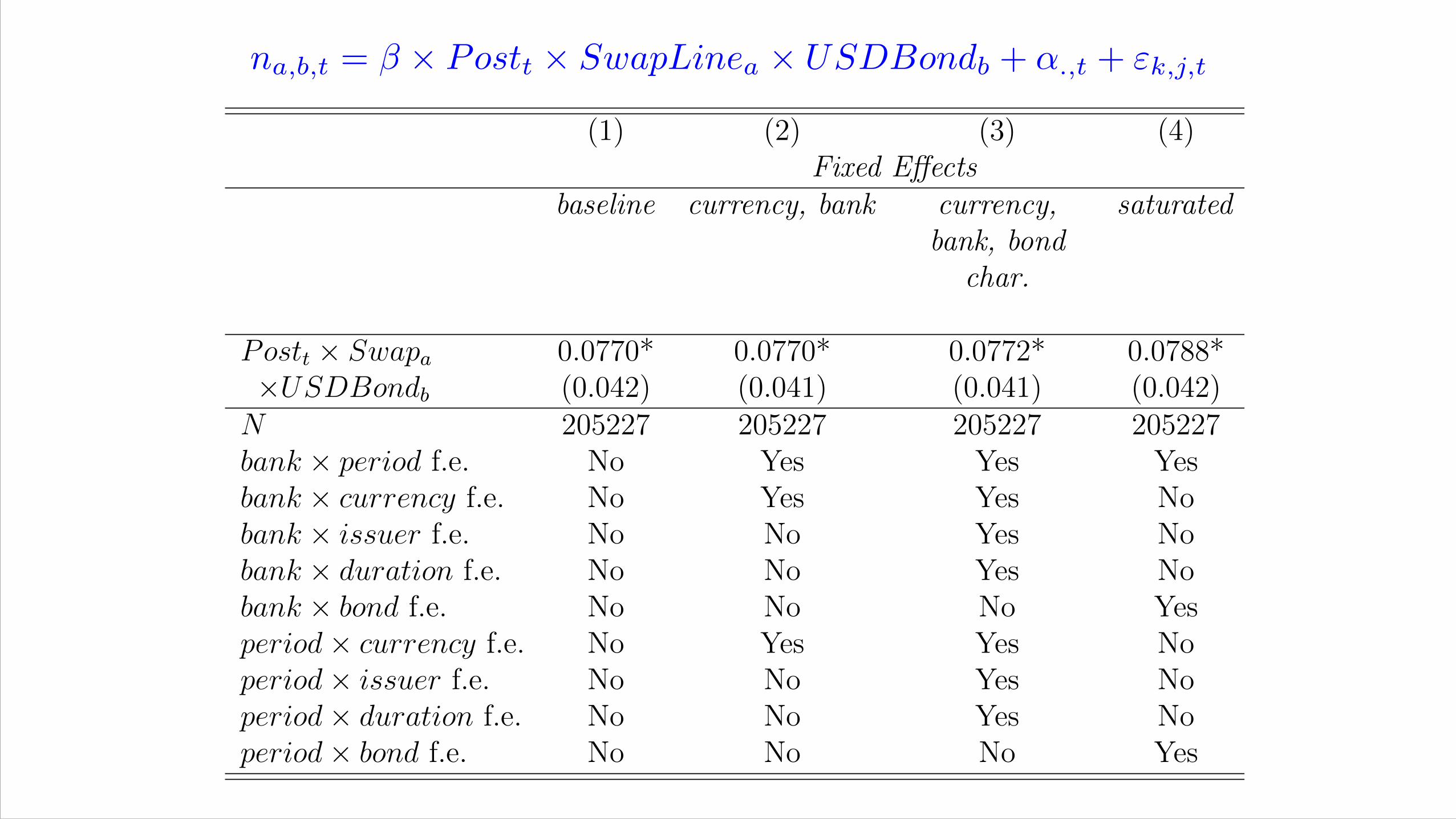
Table 4: Fixed-e↵ects panel regression estimates of the e↵ect of swap line rate changes on investment flows

(1) (2) (3) (4) (5) (6) (7)Fixed E↵ects Alternative Samples

baseline currency, bank currency,bank, bond

char.

saturated include in-frequentlytradingbanks

high rating(A- andabove)

low rating

Post

t

⇥ Swap

a

0.0770* 0.0770* 0.0772* 0.0788* 0.1033 0.0759 0.0756*⇥USDBond

b

(0.042) (0.041) (0.041) (0.042) (0.062) (0.064) (0.042)N 205227 205227 205227 205227 284225 101796 103431bank ⇥ period f.e. No Yes Yes Yes Yes Yes Yesbank ⇥ currency f.e. No Yes Yes No No No Nobank ⇥ issuer f.e. No No Yes No No No Nobank ⇥ duration f.e. No No Yes No No No Nobank ⇥ bond f.e. No No No Yes Yes Yes Yesperiod⇥ currency f.e. No Yes Yes No No No Noperiod⇥ issuer f.e. No No Yes No No No Noperiod⇥ duration f.e. No No Yes No No No Noperiod⇥ bond f.e. No No No Yes Yes Yes Yes

Notes: Estimates of equation (9). The dependent variable is n

a,b,t

, bond level daily flows by bank scaled by the total absolute flow by bank.

Post

t

is a dummy variable taking a value of 1 if t is after 30th of November 2011. Swap

a

is a dummy variable taking a value of 1 if the bank

a is headquartered in swap line country. USDBond

b

is a dummy variable taking a value of 1 if bond b is dollar denominated. Column (1):

triple di↵erence estimator, including Swap

a

⇥ period, USDBond

b

⇥ period and Swap

a

⇥ USDBond

b

fixed e↵ects. Column (2): adds bank

specific and bond-currency specific fixed e↵ects. Column (3): additionally adds issuer and duration (3-year window) fixed e↵ects. Column (4):

saturated regression. Column (5): includes in the sample banks who trade infrequently. Column (6): limits the sample to bonds that are rated

A- and above. Column (7): limits the sample to bonds that are rated BBB+ and below. Standard errors, clustered at the bank and bond level,

are in brackets. *** denotes statistical significance at the 1% level; ** 5% level;* 10% level.

28

Effect on bond prices

Table 5: Impact of swap line rate change on the yield of frequently-traded USD-denominatedbonds

Nearest Exact Match on DroppingNeighbor Euro Issuers Euro-area Issuers

foreignheld

b

-0.0860** -0.1221*** -0.1264***(0.036) (0.036) (0.038)

N 5474 5474 5257

Notes: The dependent variable is the change in the average yield of the bond in the 5 trading days following

the swap rate change on the 30th of November 2011, versus the 5 days before. The independent variable is

a dummy for whether the bond is frequently traded by our sample of European banks. Column (1): nearest

neighbor estimates, using Abadie and Imbens (2011) bias correction, that single matches on five bond char-

acteristics: (i) credit rating, converted into a numerical scale, (ii) log residual maturity, (iii) coupon, (iv) log

of the face value outstanding, and (v) average yield in the 5 days prior to 30th November. Column (2): exact

matching estimators that requires the bond issuer to be located in a Euro-area country. Column (3): Drops

bonds issued by Euro-area firms. Robust standard errors are in brackets. *** denotes statistical significance

at the 1% level; ** 5% level;* 10% level.

excess returns around the swap-rate change dates. Again, this is a triple-di↵erence exercise,

that compares: (i) the days before and after the swap-line rate change by the Fed, (ii) foreign

banks in countries covered by the dollar swap lines and so a↵ected by the rate change, and

(iii) foreign banks with a U.S. presence versus foreign banks with no U.S. investments. The

theory predicts that only the global banks with a U.S. presence should be a↵ected by the

change in the swap line terms.

Turning to the data, we define a bank as having a U.S. presence if it appears in the “U.S.

Branches and Agencies of Foreign Banking Organizations” dataset compiled by the U.S.

Federal Institutions Examination Council. Ideally, we would like to measure the exposure of

a bank to dollar funding shocks, or its reliance on U.S. wholesale funding. The presence of

a branch is only an imperfect proxy for this, so estimates will not be very precise.

We match banks to their equity returns taken from Datastream. Excess returns are

computed as the component of each bank’s returns unexplained by the total market return

in the country where the bank is based, where the relevant betas are computed over the 100

trading days ending on the 31st October 2011. The window after the announcement over

which the excess returns are cumulated is five days.

Figure 9 presents the results. It compares the average excess returns for banks in the

31

• Nearest Neighbour estimator on similar USD bonds outside the sample of frequently traded bonds:• 8bp fall in average yields in five day window after announcement. • Not driven by Euro area issuers most likely to benefit.

Returns around swap rate line change

Conclusion• Central bank swap lines: large and integral.

• Swap line is the twin of the discount window when foreign banks invest and borrow domestically

• Swap line spread plus foreign difference between policy and deposit central bank rates put ceiling on CIP deviations, empirically there from both variations.

• Swap line encourages investment in dollar assets ex ante, prevents fire sales ex post. Empirically see portfolio tilt towards bonds, increase in price of USD bonds traded by foreigners, increase in share price of foreign banks.

• Overall: eased funding pressure in cost of hedging foreign funding, choice of investments to fund, asset prices of those investments, stock price of investors

Appendix Material

• Further features:• Triple difference allows us to control for bond specific factors, like shocks to the issuer’s

credit worthiness, and to identify shifts in preferences among banks for bonds of different denominations.

• Stronger effect on lower credit ratings, stronger effect for infrequent traders

• How large was effect of 0.5% fall in swap line rate?• Within sample, increase in gross flows of $230 million, 4.8% of their absolute flow.• Extrapolating out of sample to all bonds issued by U.S. non-financial excluding the

government in the flow of funds: $8.31 billion shift in capital flows.

Features and how large

Swap dollar funding allocation

Elasticity of allotment to gain

focusing on the 10th percentile.10 The e↵ect is similar. A caveat is that over the whole

sample, the 10th percentile of observations includes some that violate the ceiling; see Figure

2 for the Euro and sterling. The third column therefore instead runs a censored regression,

including only observations if the CIP deviations were in the 90th percentile of their sample

distribution. As expected, the estimates are much larger: near the ceiling, a fall in 1%

in the ceiling lowers the CIP deviations by 66bp. Finally, the fourth column adds a time

fixed e↵ect. This removes the variation from the Fed’s actions, so that all that is left is the

variation from changes in deposit rates by the recipient central banks. The estimate falls to

11bp, consistent with a downward bias due to reverse causality.

3.5 Estimating the demand for funding liquidity by foreign banks

Let qj,t be the flow of dollars allocated by a central bank in swap line country j at an auction

at date t. If the ceiling was never met for any bank, then qj,t should always be zero. However,

there is considerable bank variation in quoted forward rates (Cenedese, Corte and Wang,

2017), leading a few banks to hit the ceiling and therefore ask for dollars from their national

central bank. Figure 5 shows the allotment for the ECB and Bank of Japan auctions, which

had significant amounts outstanding throughout the sample.11

Our next empirical test is to estimate the following regression for one-week dollar auctions:

log(qj,t) = ↵j + �jxj,t�1 + "j,t. (5)

The terms of these dollar auctions were announced in advance and were well known at most

auction dates. Moreover, these were full allotment auctions, where banks could obtain as

much funding as they wanted at this rate. Thus the supply of dollars was horizontal and

known. Therefore, this regression identifies the demand curve for central bank liquidity.

Table 3 shows the results. The elasticity of demand for dollars by European banks

is 2.2%, while that by Japanese banks is 2.5%. Both elasticities are positive, as the theory

predicts, and surprisingly close to each other. The last column of the table present a di↵erent

estimate, of the elasticity of euros lent out by the ECB in its 1 week auctions with respect

to the marginal cost of funds, the 1 week euro Libor-OIS spread. The elasticity of domestic

funding of euros by the ECB with respect to its cost is 1.62%, not statistically significantly

10While panel quantile regressions su↵er from an incidental parameters problem, the bias should be smallin our very large sample.

11The BoJ commenced 1 week auctions on the 29th of March 2011. Zero values are recoded after logarithmsto zero.

15

Table 3: Auction allotments and funding costs

ECB: USD Auctions BoJ: USD Auctions ECB: EUR Auctionslog(q

j,t

) log(qj,t

) log(qj,t

)x

j,t�1 : CIP Deviation 2.2353*** 2.4262***(0.527) (0.9891)

x

j,t�1 : 1-week Libor-OIS 1.5804***(0.587)

N 217 90 388Adjusted R

2 0.08 0.14 0.14

Notes: Estimates of equation (6). CIP deviation is the 1-week EUR or JPY vis-a-vis the USD on the day

prior to the auctions. We consider auctions where a positive amount is alloted between the 19th September

2008 (the date of the first multilateral Federal Reserve swap agreement) through to 31st December 2015.

Robust standard errors are in brackets. *** denotes statistical significance at the 1% level; ** 5% level;*

10% level.

predicts, and surprisingly close to each other. The last column of the table presents a

di↵erent estimate, of the elasticity of euros lent out by the ECB in its 1 week auctions with

respect to the marginal cost of funds, the 1 week euro Libor-OIS spread. The elasticity is

1.6%, not statistically significantly di↵erent from the elasticity of demand for dollars from

the ECB by the same set of banks. This confirms the tight link between conventional lending

facilities and the unconventional swap lines that was the main result of section 2.

4 The macroeconomic e↵ects of the swap lines

We have so far established that the central bank swap lines are a lending facility, similar to

the conventional discount window, but used by foreign banks, and that changes in the swap

rate transmit through financial markets via the price of exchange-rate forward contracts and

the associated deviations from CIP. This section shows, in theory and in the data, that this

has macroeconomic e↵ects in the investment decisions of firms and the risks they face.

4.1 A simple model of global banks’ investment decisions

Consider a simple model of funding risk a↵ecting banks that live for three periods. There

are two countries: a source country and a recipient country, with source and recipient cur-

rencies respectively. The source-country central bank provides a swap line, through which a

recipient-country bank can borrow source currency at the rate i

s.

19