Bank of Canada staff working papers provide a forum for staff to publish work-in-progress research independently from the Bank’s Governing Council. This research may support or challenge prevailing policy orthodoxy. Therefore, the views expressed in this paper are solely those of the authors and may differ from official Bank of Canada views. No responsibility for them should be attributed to the Bank.

www.bank-banque-canada.ca

Staff Working Paper/Document de travail du personnel 2018-36

Central Bank Digital Currency and Monetary Policy

S. Mohammad R. Davoodalhosseini

ISSN 1701-9397 © 2018 Bank of Canada

Bank of Canada Staff Working Paper 2018-36

July 2018

Central Bank Digital Currency and Monetary Policy

by

S. Mohammad R. Davoodalhosseini

Funds Management and Banking Department Bank of Canada

Ottawa, Ontario, Canada K1A 0G9 davo@bankofcanada.ca

i

Acknowledgements

I would like to thank Jonathan Chiu, Charles Kahn and Francisco Rivadeneyra for their

helpful comments and suggestions. I would also like to thank Wilko Bolt, Pedro Gomis-

Porqueras, Scott Hendry, Janet Jiang, Todd Keister, Sephorah Mangin, Venky

Venkateswaran, Steve Williamson, Cathy Zhang, Yu Zhu, and the participants in the

seminars at the Bank of Canada: Monash University; Central Bank Research Association;

the Summer Workshop on Money, Banking, Payments and Finance; and the workshop of

the Australasian Macroeconomics Society.

The views expressed in this paper are solely those of the author and no responsibility for

them should be attributed to the Bank of Canada.

ii

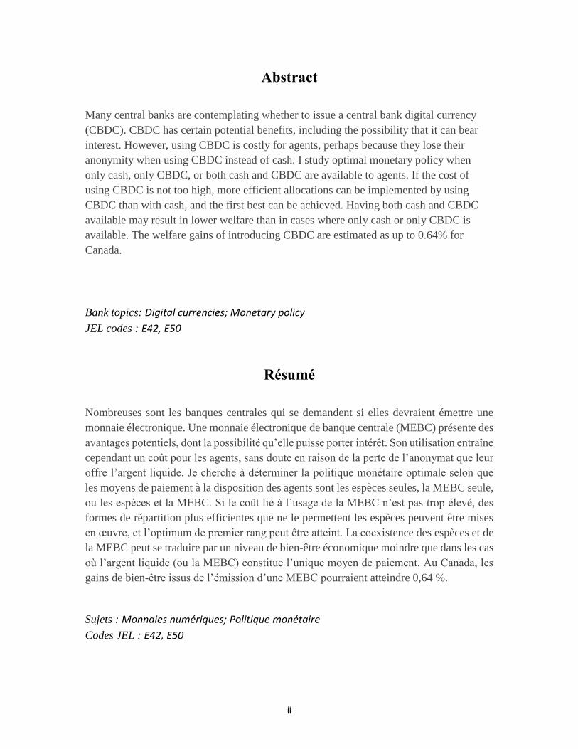
Abstract

Many central banks are contemplating whether to issue a central bank digital currency

(CBDC). CBDC has certain potential benefits, including the possibility that it can bear

interest. However, using CBDC is costly for agents, perhaps because they lose their

anonymity when using CBDC instead of cash. I study optimal monetary policy when

only cash, only CBDC, or both cash and CBDC are available to agents. If the cost of

using CBDC is not too high, more efficient allocations can be implemented by using

CBDC than with cash, and the first best can be achieved. Having both cash and CBDC

available may result in lower welfare than in cases where only cash or only CBDC is

available. The welfare gains of introducing CBDC are estimated as up to 0.64% for

Canada.

Bank topics: Digital currencies; Monetary policy

JEL codes : E42, E50

Résumé

Nombreuses sont les banques centrales qui se demandent si elles devraient émettre une

monnaie électronique. Une monnaie électronique de banque centrale (MEBC) présente des

avantages potentiels, dont la possibilité qu’elle puisse porter intérêt. Son utilisation entraîne

cependant un coût pour les agents, sans doute en raison de la perte de l’anonymat que leur

offre l’argent liquide. Je cherche à déterminer la politique monétaire optimale selon que

les moyens de paiement à la disposition des agents sont les espèces seules, la MEBC seule,

ou les espèces et la MEBC. Si le coût lié à l’usage de la MEBC n’est pas trop élevé, des

formes de répartition plus efficientes que ne le permettent les espèces peuvent être mises

en œuvre, et l’optimum de premier rang peut être atteint. La coexistence des espèces et de

la MEBC peut se traduire par un niveau de bien-être économique moindre que dans les cas

où l’argent liquide (ou la MEBC) constitue l’unique moyen de paiement. Au Canada, les

gains de bien-être issus de l’émission d’une MEBC pourraient atteindre 0,64 %.

Sujets : Monnaies numériques; Politique monétaire

Codes JEL : E42, E50

1

Non-technical summary

Many central banks are contemplating whether to issue central bank digital currency (CBDC). If they do, CBDC will co-exist with other means of payment, including cash. On one hand, CBDC has certain potential benefits, including the possibility that it can bear interest. On the other hand, cash may be preferred by agents over CBDC, perhaps because they can remain anonymous in transactions by using cash.

Interactions between cash and CBDC have not been well understood in the literature. I put together a model in which cash and CBDC co-exist, and agents with heterogeneous transaction needs can choose their portfolios with varying mixtures of each. Using this model, I investigate how monetary policy is affected by the introduction of CBDC, and study the circumstances under which its use is desirable. I show that CBDC provides more flexibility for the central bank to conduct monetary policy. This is because the central bank can monitor agents' portfolios of CBDC and can cross-subsidize between different types of agents, but these actions are not possible if agents use cash.

Having both cash and CBDC available to agents sometimes results in lower welfare than in cases where only cash or only CBDC is available. This fact suggests that removing cash from circulation may be a welfare-enhancing policy if the motivation to introduce CBDC is to improve monetary policy effectiveness. When the availability of both cash and CBDC results in higher welfare than in the above-mentioned cases, optimal cash inflation is strictly positive, and agents endogenously use cash in small-value transactions and CBDC in large-value transactions.

The welfare gains of introducing CBDC are estimated as up to 0.64% for Canada.

“[P]hasing out paper currency is arguably the simplest and most elegant approach to

clearing the path for central banks to invoke unfettered negative interest rate policies should

they bump up against the ‘zero lower bound’ on interest rates.”

Ken Rogoff (2016) in The Curse of Cash

“Some economists advocate that the central bank should replace cash with a digital cur-

rency that can be given a negative interest rate. ... This reasoning is based on the central

bank being prevented from setting a negative interest rate to the extent considered necessary

to stimulate economic activity. Personally, I am not convinced that this problem would arise

in Sweden and I would once again like to say that the Riksbank has a statutory requirement

to issue banknotes and coins. I see e-krona primarily as a complement to cash.”

Skingsley (2016), Deputy Governor of the Bank of Sweden

1 Introduction

There has been a great deal of discussion in recent years about the effects of introducing

central bank digital currency (CBDC) into economies and whether cash should be eliminated,

as the quotes above indicate. Some central banks have already started the decision-making

process on whether to introduce CBDC into their respective economies. For example, the

central bank of Sweden wants to decide soon on whether to issue CBDC (what they call

“e-krona”), and if yes, what type of CBDC.1 Also, some officials at the central bank of

China have expressed their desire to issue their own digital currency as a way to support

their digital economy.2 If central banks issue CBDC, important questions arise, some of

which are as follows: Should central banks eliminate cash from circulation? What would

be the optimal (i.e., welfare-maximizing) monetary policy if agents can choose between cash

and CBDC? And quantitatively, what are the welfare gains of introducing CBDC into the

economy?3

1See the first interim report on the Riksbank’s E-krona Projects (Sveriges Riksbank (2017)). Also note

that CBDC can be of different types. Several authors have suggested taxonomies to understand various

types of electronic money, some forms of which are CBDC. See Bech and Garratt (2017), Bjerg (2017) or

the Committee on Payments and Market Infrastructures (2015) report on digital currencies.2See here: https://goo.gl/kEpHhV.3It may seem that these questions are about the payment systems only, but the endogenous choice of

means of payment by agents affects the optimal monetary policy that the central bank can adopt and,

consequently, welfare.

2

To address these and similar questions, I use the framework of Lagos and Wright (2005) to

build a model in which two means of payment could be available to agents: cash and CBDC.

What I mean by CBDC in this paper is the money issued by the central bank in electronic

format and universally accessible; i.e., all agents in the economy can use it to purchase goods

and services.4 I study the optimal monetary policy when only one or both means of payment

are available to agents. Cash and CBDC are different along two dimensions in this paper.

First, the ability of the central bank to implement monetary policy is different across these

means of payment. The central bank can allocate transfers to agents based on their CBDC

balances but the central bank cannot do so based on their cash balances because the central

bank cannot see agents’ cash balances. Therefore, the only policy that the central bank

can implement with cash is to distribute the newly created cash evenly across all agents.5

Second, carrying CBDC is more costly relative to cash. This cost is perhaps due to the fact

that agents lose their anonymity if using CBDC. This cost creates a sensible tradeoff for the

central bank regarding the means of payment that the central bank would like agents to use.

While CBDC is a more flexible policy instrument, it is more costly than cash.

There are two main results of the paper. First, given that the cost of carrying CBDC

is sufficiently small, the fact that CBDC is interest bearing in a non-linear fashion allows

the central bank to achieve better allocations than with cash. In particular, it is possible to

achieve the first-best level of production by using CBDC if the agents are patient enough

and if the bargaining power of buyers is sufficiently high, while it is never possible to achieve

the first best by using cash. Second, when cash and CBDC are both available to agents and

valued in equilibrium, the monetary policy may be more constrained (i.e., welfare may be

lower) compared with the case in which only one means of payment is available.

To elaborate on these results, consider three different schemes: only cash is available to

the agents (cash-only scheme), only CBDC is available to the agents (CBDC-only scheme),

and both cash and CBDC are available (co-existence scheme).6 If only cash is available,

then the optimal inflation in this economy is zero. It would not be possible to implement

a negative inflation as the central bank cannot force agents to pay taxes, and a positive

4A similar form of money was proposed by Tobin (1987). In his own words: “I think the government

should make available to the public a medium with the convenience of deposits and the safety of currency,

essentially currency on deposit, transferable in any amount by check or other order.”5It is important to note that taxing cash balances is not feasible here; otherwise, the central bank can

simply run the Friedman rule to achieve the first best, and adding CBDC or replacing cash by CBDC would

not offer any potential improvements.6The optimal monetary policy under co-existence is defined to be one that maximizes welfare among all

policies under which both cash and CBDC are valued in equilibrium and used as means of payment.

3

inflation would lead agents to economize on their real balances relative to the first best, so

the production level is distorted. If only CBDC is available, then the set of implementable

allocations is larger, because the balance-contingent transfers are allowed with CBDC, not

with cash, and even the first-best level of production can be achieved. However, there is

welfare loss resulting from the cost of carrying CBDC. Comparing cash-only and CBDC-

only schemes, we find that the tradeoff for the central bank is simply between distorting the

allocation relative to the first best under the cash-only scheme or having the agents incur

the cost of carrying CBDC under the CBDC-only scheme.

Under the co-existence scheme, agents with lower transaction needs endogenously choose

to use cash, and agents with higher transaction needs choose to use CBDC. In this case, the

central bank faces a constraint stemming from the endogenous choice of means of payment.

Because cash is available, agents who would have used CBDC if cash had not been available

can now use cash as a way to evade the taxation that CBDC users are subjected to. To

discourage these agents from using CBDC, the central bank could set the cash inflation too

high, but it would hurt cash users. Therefore, the availability of cash in the presence of

CBDC imposes a constraint for the central bank’s maximization problem. Whether or not

the co-existence scheme is optimal (i.e., leading to higher welfare) relative to cash-only or

CBDC-only schemes depends on how tight this constraint is. If the constraint is too tight,

then the central bank would prefer to have only one means of payment used by agents. In

this case, if the cost of carrying CBDC is not too high, then central bank eliminates cash,

and if the cost is too high, then the central bank eliminates CBDC. On the other hand, if

the constraint is relatively relaxed, then the central bank would have both cash and CBDC

circulating in the economy.

For both cash and CBDC to be used by agents, the cash inflation must be strictly

positive. This result is obtained despite the fact that it is feasible to implement a negative

cash inflation rate when both are available (through open market operations where cash is

traded for CBDC), but it would induce CBDC users to use cash instead. Therefore, CBDC

would not be adopted under a negative cash inflation rate.

Rogoff (2016) has argued in favor of eliminating cash from circulation, except perhaps for

small-denomination notes, as the first quote above indicates. One of his main arguments is

that by eliminating cash, central banks can stimulate the economy in downturns via setting

negative nominal interest rates. If cash is available, since cash guarantees the nominal

interest rate of zero for agents, the ability of central banks to stimulate the economy will

be restricted. The reason that co-existence of cash and CBDC may not be optimal in my

model is similar to Rogoff’s argument. In both, cash provides an outside option for agents,

4

restricting the set of feasible allocations that the central bank can achieve. However, it is

important to note that the effectiveness of CBDC is not only due to the fact that it allows

for the possibility of achieving negative interest rates, but it also allows for implementation

of non-linear transfer schemes, the feature that I use to show that the first-best level of

production can be achieved using CBDC. Furthermore, CBDC provides more information

to the central bank, such as whether the agent is a buyer or seller or the size of transaction.

Altogether, even if cash is not eliminated, CBDC can still positively affect monetary policy,

although its effectiveness is sometimes enhanced if cash is eliminated.7

To give a sense of the welfare gains of introducing CBDC, I calibrate the model to the

Canadian and US data. I show that introducing CBDC can lead to an increase of up to

0.64% in consumption for Canada and up to 1.6% for the US, compared with their respective

economies if only cash is used. Assuming that there are only two sizes of transactions (large-

value and small-value transactions), I calculate the welfare gains of introducing CBDC for

different values of the cost of carrying CBDC and for various values of the relative size of

large- to small-value transactions. As an example, if the monetary cost of carrying CBDC

relative to cash is 0.25% of the transaction value and the average value of large transactions

is around six times the size of small-value transactions, then introducing CBDC will lead to

an increase in consumption of 0.16% for Canada.

In an extension of the benchmark model, I assume that CBDC is not a perfect substitute

for cash, in that CBDC cannot be used in a fraction of transactions in which cash can be

used. In this case, if the cost of carrying CBDC is low, then co-existence might be optimal.

Also, the first best can be achieved as long as the fraction of meetings in which only CBDC

can be used and also the discount factor are sufficiently high. This result shows, interestingly,

that CBDC helps to achieve the first best even for the meetings in which only cash can be

used.

One may argue that the type of CBDC addressed in this paper is difficult to implement

in practice because the interest payments suggested here are traditionally in the realm of

fiscal policy, not monetary policy. This argument ignores two facts: First, the central banks

in most advanced economies already make interest payments on reserves, but only to some

financial institutions that have exclusive access to the central bank facilities. Second, those

interest payments are non-linear in that the interest rate paid on reserves is different from

7Another point is that in Rogoff’s argument, the policy of negative nominal interest rates is needed for

short-run stabilization. In contrast, I analyze the steady state of the model, and the interests paid on CBDC

balances are aimed at maximizing the long-term welfare of the population, not stabilizing the economy in

the short run.

5

the rate charged to borrowers. Central banks have recognized that the payments on reserves

in the current system can serve their policy objectives, so why not extend access to all agents

if economic efficiency requires that?8

The rest of the paper is organized as follows. After briefly discussing the related literature,

I lay out the model in Section 2. I assume in all sections except Section 7 that cash and

CBDC are perfect substitutes; i.e., both can be used in all transactions. In Section 3 and as

a benchmark, I assume cash and CBDC are both costless to carry. In Section 4, I assume

CBDC is more costly to carry relative to cash. I show, among other results, that if both

cash and CBDC are used by agents under the optimal policy, cash is used in small-value

transactions and CBDC is used in large-value transactions. In Section 5, I focus on a

special case in which there are only two sizes of transactions—large-value and small-value

transactions—and characterize conditions under which cash and CBDC are both used by

agents under the optimal policy. In Section 6, I calibrate the model to the Canadian and US

data to estimate the welfare gains of introducing CBDC into these economies. In Section 7,

I assume that cash and CBDC are not perfect substitutes in that in a fraction of meetings,

only cash can be used, and in a fraction of meetings, only CBDC can be used. I show here

that co-existence may be welfare enhancing relative to cash-only or CBDC-only schemes.

Section 8 concludes.

Related Literature. This paper is related to the monetary theory literature, especially

the models that emphasize the micro-foundations of money. The model is built on the

framework developed by Lagos and Wright (2005) and Rocheteau and Wright (2005), and

has the same structure of a centralized market (CM) and a decentralized market (DM). The

CBDC in my paper is similar to the interest-bearing money in Andolfatto (2010). However,

he does not study the endogenous choice of means of payment when (non-interest-bearing)

cash and interest-bearing money are both available to agents; nor does he have idiosyncratic

preference shocks that lead to endogenous adoption of different means of payment by agents

with different transaction needs in my paper.

A closely related paper is Chiu and Wong (2015). They show that electronic money allows

the first-best allocation to be implemented under a broader set of parameter values relative to

cash.9 Another related paper is Gomis-Porqueras and Sanches (2013), in which there are two

payment systems—fiat money and credit—and there is a cost effectively incurred by buyers

8Furthermore, I take the implementation of monetary policy more seriously than most papers in monetary

economics where the creation of new money is assumed to be done through helicopter drop (lump-sum

transfers). In my model, the implementation is done either through open market operations (exchange of

cash with CBD) or through direct transfers to CBDC accounts.9I elaborate in the appendix on the differences between my paper and some closely related papers.

6

to access the credit system. The credit system in their paper is similar to the CBDC in my

paper. Dong and Jiang (2010) show that two monies can expand the set of parameters for

which the first best is achievable in an environment in which agents have private information

about their preference types. Zhu and Hendry (2017) study currency competition between

cash and privately issued digital currency. They show that if the private issuer is not welfare

maximizing, there will be coordination problems between the central bank and the private

issuer and welfare will be lower relative to the case in which the central bank has full control

of monetary policy.10 In other models in the literature, money and credit are studied in

the same model (like Gu et al. (2016) and Chiu et al. (2012)). Using credit is not possible

in my model, as the central bank cannot keep track of the agents’ actions in the DM. The

central bank observes only the agents’ balances at the end of the CM. My model is also

related to Rocheteau et al. (2014) in that in both papers, an open market operation (OMO)

is used. OMO is used in my model as a cross-subsidization device between cash and CBDC

users. Finally, on estimating the costs and benefits of issuing CBDC, Barrdear and Kumhof

(2016) estimate that CBDC issuance could increase GDP by as much as 3%, mostly through

lowering the real interest rates.

2 Model

The model is based on Lagos and Wright (2005), LW hereafter, with two means of payment:

cash and CBDC. I use index c to refer to cash and index e (for electronic money) to refer

to CBDC. Time is discrete: t = 0, 1, 2, .... Each period consists of two subperiods: DM and

CM. In the DM, a decentralized market, and in the CM, a decentralized market, is active.

There is a continuum of buyers and continuum of sellers, each with a unit mass. Both have

discount factor β ∈ (0, 1) from CM to DM. In the CM, both can consume and produce. In

the DM, sellers can only produce and buyers can only consume. In the CM, one unit of

labor supply produces one unit of perishable consumption good. In the DM, a buyer and

seller meet randomly with probability σ and split the gains from trade based on proportional

10There is a growing body of literature studying CBDC and its implications for the payment systems,

monetary policy implementation and financial stability. I cannot do justice to all the papers in this literature,

but to mention only some examples, Fung and Halaburda (2016) study a framework to assess why a central

bank should issue digital currency. Kahn et al. (2017) study different schemes of CBDC and discuss how

these schemes can meet the central bank’s objectives. Finally, Berentsen and Schar (2018) argue in favor of

central banks issuing CBDC. In particular, they argue that implementing monetary policy using CBDC is

more transparent than the current way of implementing monetary policy.

7

bargaining. The buyer’s utility function is given by:

E0

∞∑t=0

βt(wtu(qt) +Xt),

where buyer’s preference shock, wt, is an i.i.d. draw across time and agents from CDF F (w)

and w ∈ [wmin, wmax], u(q) is the utility of consuming q units of the DM good, and Xt is the

consumption of numeraire in the CM. Introducing this preference shock is the first departure

from the standard LW model. The seller’s utility function is given by:

E0

∞∑t=0

βt(−c(qt) +Xt).

where c(q) is the cost of producing q units of the DM good. Sellers do not receive a preference

shock. All interesting actions come from the buyers’ decisions in this paper. I assume that

u′′ < 0 < u′, u(0) = 0 and 0 < c′′, 0 < c′, c(0) = 0. Clearly, the first-best production level for

type w is given by:

q∗w = arg maxq{wu(q)− c(q)}.

Another departure from the standard LW model is that there are two means of payment

in this economy—cash and CBDC. Denote by ce(ze) : R+ → R+ the cost of carrying ze units

of real balances (in terms of the CM good) in the form of CBDC from CM to DM. It is

assumed that the buyer incurs this cost. The cost of carrying real balances in the form of

cash is assumed to be zero.

The timing of actions and realization of shocks in period t are specified as follows. In

the DM, agents are randomly matched and trade according to the proportional bargaining

protocol, with θ ∈ [0, 1] being the share of the buyer. In the bilateral meeting, w is known

both to the buyer and seller, so there is no problem regarding private information. After

agents trade in the DM and get separated from the match, the buyers learn their w for the

next period. Next, agents trade in the CM. They work and choose the amount of CBDC

and cash they want to carry to the next DM. At the end of the CM, new cash and CBDC

are transferred to agents as will be described below. Denote by zc ∈ R+ the number of

pre-transfer real balances in the form of cash. Similarly, denote by ze ∈ R+ the number of

pre-transfer real balances in the form of CBDC. Denote by tc ∈ R+ the helicopter drop of

cash in real terms (units of the CM good) to all buyers. Denote by te(ze, w) : R+ → R+ the

number of CBDC transfers in real terms to type w buyers that have brought ze from the CM.

It is assumed that the planner has complete information about the buyer’s type if the buyer

uses CBDC. Yet, the only feasible policy using cash is a helicopter drop. This assumption

8

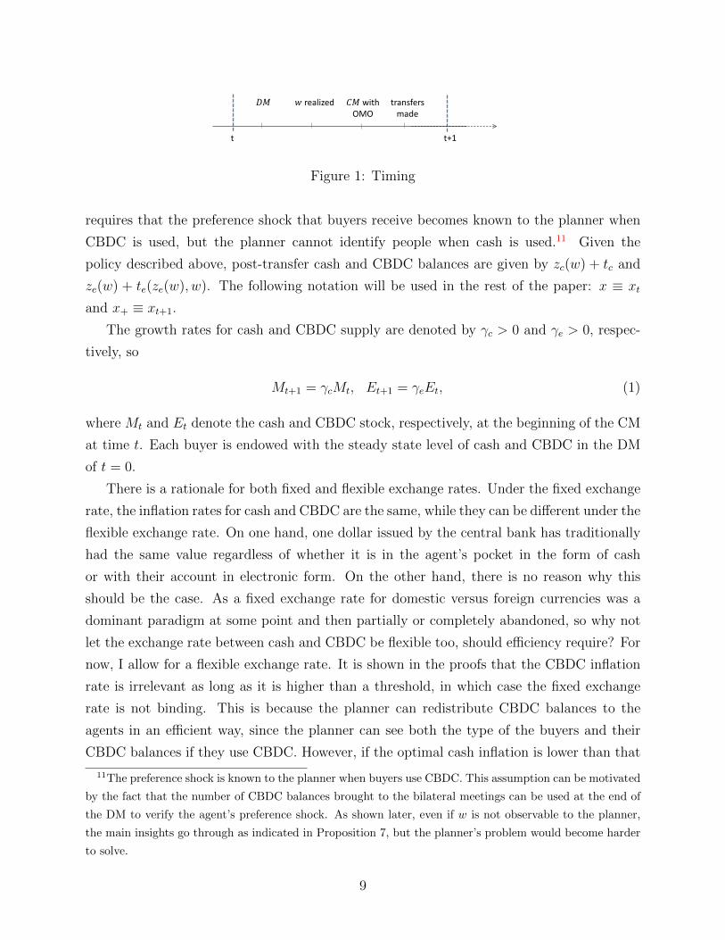
t t+1

𝐷𝐷 𝑤 realized 𝐶𝐷 with OMO

transfers made

Figure 1: Timing

requires that the preference shock that buyers receive becomes known to the planner when

CBDC is used, but the planner cannot identify people when cash is used.11 Given the

policy described above, post-transfer cash and CBDC balances are given by zc(w) + tc and

ze(w) + te(ze(w), w). The following notation will be used in the rest of the paper: x ≡ xt

and x+ ≡ xt+1.

The growth rates for cash and CBDC supply are denoted by γc > 0 and γe > 0, respec-

tively, so

Mt+1 = γcMt, Et+1 = γeEt, (1)

where Mt and Et denote the cash and CBDC stock, respectively, at the beginning of the CM

at time t. Each buyer is endowed with the steady state level of cash and CBDC in the DM

of t = 0.

There is a rationale for both fixed and flexible exchange rates. Under the fixed exchange

rate, the inflation rates for cash and CBDC are the same, while they can be different under the

flexible exchange rate. On one hand, one dollar issued by the central bank has traditionally

had the same value regardless of whether it is in the agent’s pocket in the form of cash

or with their account in electronic form. On the other hand, there is no reason why this

should be the case. As a fixed exchange rate for domestic versus foreign currencies was a

dominant paradigm at some point and then partially or completely abandoned, so why not

let the exchange rate between cash and CBDC be flexible too, should efficiency require? For

now, I allow for a flexible exchange rate. It is shown in the proofs that the CBDC inflation

rate is irrelevant as long as it is higher than a threshold, in which case the fixed exchange

rate is not binding. This is because the planner can redistribute CBDC balances to the

agents in an efficient way, since the planner can see both the type of the buyers and their

CBDC balances if they use CBDC. However, if the optimal cash inflation is lower than that

11The preference shock is known to the planner when buyers use CBDC. This assumption can be motivated

by the fact that the number of CBDC balances brought to the bilateral meetings can be used at the end of

the DM to verify the agent’s preference shock. As shown later, even if w is not observable to the planner,

the main insights go through as indicated in Proposition 7, but the planner’s problem would become harder

to solve.

9

threshold, then imposing a fixed exchange rate will be a binding restriction for the planner’s

problem, leading to a less efficient allocation.12

We focus on the cases where total real cash and CBDC balances are constant over time:

φtMt = φt+1Mt+1 and ψtEt = ψt+1Et+1. This implies that:

φtφt+1

= γc,ψtψt+1

= γe. (2)

I allow the planner to use OMO to change the relative supply of cash and CBDC. By OMO,

I mean that the government trades CBDC for cash in the CM with the price ψφ

. In that case,

the equilibrium conditions can be written as follows:

M −M = −ψφ

(E − E), (3)

tc = φ+(M+ − M), (4)∫te(ze(w), w)dF (w) = ψ+(E+ − E), (5)∫

zc(w)dF (w) = φ+M, (6)∫ze(w)dF (w) = ψ+E, (7)

where M and E are the cash and CBDC supply after the OMO and before transfers are

made to the agents, and zc(w) and ze(w) are real balances of cash and CBDC that a buyer

of type w holds in the steady state.

Equation (3) states that the net number of real balances supplied to the CM in the form

of cash and CBDC is equal to 0. Equations (4) and (5) simply pin down the value of transfers

in the form of cash and CBDC, respectively, available to be distributed across agents. For

example, tc is the real value of balances in CMt+1 given to buyers in the transfer stage of

period t. Equations (6) and (7) are market-clearing conditions for cash and CBDC.

Two points about OMO are worth mentioning. First, (3) shows that OMO is a cross-

subsidization tool between cash and CBDC users. If there is no cross-subsidization, then

M = M and E = E, so tc will be pinned down by the inflation rate of cash. However,

OMO allows the amount of cash distributed among agents to be less than the amount of

newly created cash, providing a tool for the planner to achieve better allocations. Second,

12Agarwal and Kimball (2015) argue that if cash and CBDC co-exist, allowing for the exchange rate to be

different from par makes it possible to implement a negative interest rate policy. My paper and theirs share

the feature that if a flexible exchange rate between cash and CBDC is allowed, the outcome is more efficient

compared to that with a fixed exchange rate, at least under some parameters.

10

OMO can adjust the imbalances between the supplies of these two assets. Specifically, OMO

can be used for short-run stabilization in this model, as in many standard macroeconomic

models. I do not study short run-stabilization policies here, however.

Lemma 1. With OMO, the following constraint should hold in the stationary equilibrium:13

tc +

∫te(ze(w), w)dF (w) = (γc − 1)

∫zc(w)dF (w) + (γe − 1)

∫ze(w)dF (w). (8)

2.1 Agents’ Problems in the CM

Buyer’s problem in the CM:

WBw (z) = max

X,Y,zc,ze

{X − Y − ce(ze + te(ze, w)) + βV B

w (zc + tc, ze + te(ze, w))

}

s.t. X +φ

φ+

zc +ψ

ψ+

ze = Y + z,

where z denotes the real balances that the buyer has at the beginning of the CM. Also,

V Bw (zc, ze) is the value function in the DM of the buyer of type w with zc real balances in

cash and ze real balances in CBDC. Incorporating the constraint into the objective function,

one can write:

WBw (z) = z + max

zc,ze{− φ

φ+

zc −ψ

ψ+

ze − ce(ze + te(ze, w)) + βV Bw (zc + tc, ze + te(ze, w))}. (9)

The sellers’ value function in the CM can be written similarly.

2.2 Agents’ Problems in the DM

Buyers receive:

V Bw (zc, ze) = EWB

w (zc + ze)

+σ

(wu(qw(zc, ze)) + EWB

w (zc + ze − dc,w(zc, ze)− de,w(zc, ze))− EWBw (zc + ze)

)= EWB

w (zc + ze) + σ

(wu(qw(zc, ze))− dc,w(zc, ze)− de,w(zc, ze))

),

where qw(zc, ze), dc,w(zc, ze), de,w(zc, ze) denote, respectively, the production amount and the

real transfer of cash and CBDC balances in the DM meetings in which the buyer has brought

13This constraint is consolidated for both cash and CBDC. Without OMO, this condition should be

replaced by the following two constraints: tc = (γc − 1)∫zc(w)dF (w) and

∫te(ze(w), w)dF (w) = (γe −

1)∫ze(w)dF (w). In this case, the gains of CBDC would be more limited.

11

zc real balances in cash and ze real balances in CBDC. Also, the expectation is taken over

realizations of buyer types in the next period. Similarly, sellers receive:

V Sw (zc, ze) = W S(zc + ze) + σ

(− c(qw(zc, ze)) + dc,w(zc, ze) + de,w(zc, ze)

).

Superscript S represents the seller’s associated variable. The linearity of W S and WB were

used to simplify the DM value functions. Sellers do not need to bring balances to the DM

because carrying balances is costly and the sellers do not use them until the next CM.

Therefore, we focus only on the buyer’s balances, determined from the bargaining protocol.

2.3 Proportional Bargaining in the DM

Terms of trade are determined from the following maximization problem:

maxq,dc∈[−zSc ,zc],de∈[−zSe ,de≤ze]

∆B + ∆S

subject to: ∆B = θ(∆B + ∆S),

where ∆B and ∆S denote buyer’s and seller’s surplus, respectively, and are given by:

∆B ≡ V Bw (zc − dc, ze − de)− V B

w (zc, ze) + wu(q),

∆S ≡ V Sw (zSc + dc, z

Se + de)− V S

w (zSc , zSe )− c(q).

The solution to the bargaining problem is given by:14

dc,w(zc, ze) + de,w(zc, ze) = min

{zc + ze, Dw(q∗w),

}

qw(zc, ze) = D−1w

(dc,w(zc, ze) + de,w(zc, ze),

)(10)

where Dw(.) is defined as follows:

Dw(q) ≡ θc(q) + (1− θ)wu(q).

Equivalently, the solution is given by:

(qw, dc,w + de,w) =

(q∗w, Dw(q∗w)) if zc + ze ≥ Dw(q∗w)

(D−1w (zc + ze), zc + ze) otherwise

.

14This problem is basically the same as follows: maxx,d∈[−z′,z][u(x)−x] subject to u(x)−d = θ(u(x)−x).

12

In words, Dw(q) denotes the number of real balances that a type w buyer needs for buying q

units of the DM good. If the buyer brings at least Dw(q∗w), then the first best is achievable;

i.e., the first-best level of production, q∗w, can be produced. Otherwise, the buyer spends the

entire balances, and then the terms of trade are given by the second line above. Finally, the

value function for buyers and sellers at the beginning of the DM can be written as follows:

V Bw (zc, ze) = EWB

w (zc + ze) + σθ

(wu(qw(zc, ze))− c(qw(zc, ze))

),

V Sw (zc, ze) = W S(zc + ze) + σ(1− θ)

(wu(qw(zc, ze))− c(qw(zc, ze))

).

2.4 CM and DM Value Functions Together

The buyer’s problem turns into:

WBw (z) = z + EWB

w (0)

+maxzc,ze

{− φ

φ+

zc−ψ

ψ+

ze−ce(ze+te(ze, w))+β(zc+tc)+β(ze+te(ze, w))+βσθ(wu(q)−c(q))},

(11)

where q is implicitly given by Dw(q) = min{Dw(q∗w), zc + tc + ze + te(ze)}.It is standard to show that sellers do not bring any balances to the DM. In the DM, if

sellers get matched, they work to produce the DM good and sell it to the buyer, and then

bring their balances to the CM and use them to purchase the CM good and consume it.

Buyers work to acquire money (cash or CBDC) in the CM, and receive transfers from the

planner. Then, they enter the DM with the entire money stock, and exchange it all for goods

produced by sellers.

2.5 Equilibrium Definition

The equilibrium definition can now be written as follows.

Definition 1 (Stationary Equilibrium). Stationary equilibrium is a price system {φt}, {ψt},an allocation {(q(w), zc(w), ze(w))}w and a policy {γc, γe, tc, {te(ze, w)}w} such that the fol-

lowing conditions hold:

(i) Buyer’s maximization in CM: Given zc,0, ze,0, {ψt}∞t=0 and {φt}∞t=0, zc(w) and ze(w)

solve (9) (where zc,0 and ze,0 denote initial values of zc and ze).

(ii) Market clearing for cash and CBDC, planner’s budget constraint and OMO: (8) should

hold.

13

(iii) Proportional bargaining: q(w) solves (10).

(iv) Growth equation (2) for cash and CBDC.

2.6 Planner’s Problem

The planner’s problem is to maximize welfare, calculated at the beginning of the CM, by

choosing a policy:

Problem 1 (Planner’s Problem).

max{γc,γe,tc,{te(w)}w}

∫ [βσ(wu(q(w))− c(q(w))

)− ce(ze(w))

]dF (w)

subject to: {(q(w), zc(w), ze(w))}w form an equilibrium together with some prices {φt}, {ψt}and the policy.

I make the following assumption on the functional form of cash and CBDC costs through-

out the paper.

Assumption 1 (Cost Functions). CBDC costs K ≥ 0 in terms of the CM good and is to be

incurred in the CM. That is, ce(z) = KI{z > 0}.

As will be shown later, if both cash and CBDC are costless, cash is redundant, because

CBDC is a more powerful instrument for the planner to implement monetary policy. For

the planner to have a non-trivial problem regarding which means of payment should be

available to agents, CBDC needs to be disadvantageous to cash in some ways. Considering

a fixed cost of using CBDC relative to cash, as assumed here, is one way to do so. This

disadvantage is motivated by the fact that agents in the economy may value anonymity

while doing transactions, and they may lose it if they use CBDC. Also, electronic means of

payment including CBDC usually require some devices to process the payments, while cash

does not, so this cost can summarize the costs of using such devices. This disadvantage is

modeled for simplicity as a flat cost K ≥ 0 for using CBDC. The flat cost of using CBDC is

also consistent with the digital format of CBDC in that the dis-utility of losing anonymity

for the agent may be independent of the number of balances that the agent holds.

2.6.1 Simplified Planner’s Problem

The main constraint for the planner’s problem, equation (11), can be written as:

(q(w), zc(w), ze(w)) ∈ arg maxq∈[0,q∗w],zc,ze

{− (

φ

φ+

− β)(zc + tc)

14

−(ψ

ψ+

− β)(ze + te(ze, w))− ce(ze + te(ze, w)) + γctc + γete(ze, w) + βσθ(wu(q)− c(q))}

s.t. Dw(q) = min{Dw(q∗w), zc + tc + ze + te(ze, w)}.

Given the assumption on the cost functions, the planner’s problem can be simplified as

follows:

Problem 2.

max{γc,γe,tc,{te(ze,w)}}

∫ [βσ

(wu(q(w))− c(q(w))

)−KI(ze(w) > 0)

]dF (w)

s.t. (q(w), zc(w), ze(w)) ∈ arg maxq∈[0,q∗w],zc+ze+tc+te(ze,w)=Dw(q)

{−(γe−β)(ze+te(ze, w))−(γc−β)(zc+tc)+βσθ

(wu(q)−c(q))

)−KI(ze > 0)+γctc+γete(ze, w))

},

and tc +

∫(te(ze(w), w)− (γc − 1)zc(w)− (γe − 1)ze(w))dF (w) = 0.

Proposition 1. In the solution to the planner’s problem, we can assume without loss of

generality that te(z, w) is a step function in z. That is,

te(z, w) =

t0,w z ≥ z0,w

0 z < z0,w

for some t0,w ∈ R+, z0,w ∈ R+.

This lemma states that we can restrict our attention to the CBDC transfer schemes that

are step functions. That is, if an agent of type w brings at least ze(w), then he receives some

transfers, but bringing any lower real balances in CBDC does not yield him any transfers.

This is the most severe punishment of the agents by the planner.15

In the next section, I study the case in which cash and CBDC are costless as a benchmark

(K = 0). Next, I study the case in which CBDC is more costly than cash (K > 0).

15This transfer scheme can easily be implemented by a fixed fee and interest payment on balances. Follow-

ing Andolfatto (2010), assume agents are charged some fixed cost f in the CM if they want to hold CBDC

and are paid interest on their CBDC balances with i interest rate in the transfer stage. This scheme with

appropriate values for f and i can implement the same allocation as the transfer scheme here.

15

3 Costless Cash and CBDC

I show that if K = 0, cash is redundant. I also study conditions under which first best

is achievable with CBDC. It is impossible to achieve the first best with only cash, because

it is not possible to tax cash holdings nor to make transfers to agents based on their cash

holdings.

Proposition 2 (Redundancy of cash). If both cash and CBDC are costless—i.e., K = 0—

then cash is redundant. That is, any allocation that is achieved by using cash and CBDC

can be achieved by using only CBDC.

The idea is that if both cash and CBDC are costless, CBDC has a clear advantage for the

planner, as the planner can provide incentive for buyers to bring enough balances to the DM

by checking their CBDC balances. The planner can then punish agents who do not bring

enough balances from the CM by making zero transfers to them. The cash growth rate is

set sufficiently high that the gains from using cash and consequently the demand for cash

become zero.

3.1 Homogeneous Buyers

The planner sees w and can make transfers to buyers who use CBDC contingent on their

types. Cash can be distributed across agents only evenly (helicopter drop). In this section,

there is only one type so only one means of payment is generally used and a flexible exchange

rate is irrelevant for analyzing the steady state.

Proposition 3. Suppose both cash and CBDC are costless; i.e., K = 0. Suppose also the

distribution of types is degenerate at w; i.e., there is only one type. The first best is achievable

if and only if:

βσθ(wu(q∗w)− c(q∗w)) ≥ (1− β)Dw(q∗w).

The left-hand side (LHS) of the condition is the buyer’s gains from bringing the number

of balances that the planner asks for. The right-hand side (RHS) is the real cost of holding

balances. This is the inevitable cost of holding real balances with CBDC: Carrying CBDC

for buying q units of the DM good imposes (γe − β)Dw(q∗w) cost of real balances on the

buyer, but the newly created CBDC will be distributed across buyers such that they receive

(γe − 1)Dw(q∗w) real balances if they have brought enough balances. Therefore, they have

to incur the cost (1− β)Dw(q∗w). Noticeably, the inflation rate of CBDC does not affect the

incentives.

16

The condition required by this proposition is equivalent to:

θ ≥ θ(w) ≡ 1− β(1− β(1− σ))(1− c(q∗w)

wu(q∗w)).

For θ(w) ≤ 1, we must have:

β ≥(

1 + σwu(q∗w)− c(q∗w)

c(q∗w)

)−1

.

To achieve the first best, the proposition requires θ and also β to be sufficiently high. Even

in the case of θ = 1, in which the buyer takes the entire surplus, the buyer still needs to work

in the CMt to earn c(q) real balances in CBDC. The benefits of CBDC will be realized in

the DMt+1 with probability σ, in the DMt+2 with probability (1− σ)σ, and so on. For the

benefits to dominate the costs, one needs: wu(q)(βσ+β2(1−σ)σ+β3(1−σ)2σ+ ...) ≥ c(q),

which is equivalent to the above condition.16

The following proposition implies that for a given set of model parameters, there exists a

threshold for w below which the first best cannot be achieved and above which the first best

can be achieved. The condition required in this proposition is satisfied, for example, when

c(q) is linear and u(q) = (q+b)1−η−b1−η1−η where η ∈ (0, 1) and b > 0.

Proposition 4. θ(w) is decreasing in w if c′(q)u(q)c(q)u′(q)

is increasing in q.

3.2 Heterogeneous Buyers

Now suppose that the distribution of types is not degenerate. The condition in the proposi-

tion may be binding for some types and not for others. The following proposition provides

sufficient conditions to achieve the first best.

Proposition 5. Suppose both cash and CBDC are costless; i.e., K = 0. With heterogeneous

types, the first best is achievable if and only if:

βσθ

∫(wu(q∗w)− c(q∗w))dF (w) ≥ (1− β)

∫Dw(q∗w)dF (w).

Compared with the case with homogeneous buyers, cross-subsidization is possible here.

This can be seen clearly from comparing the conditions in Propositions 3 and 5. The idea is

that if the condition in Proposition 3 is slack for some types, say w2, and does not hold for

other types, say w1, the planner can charge type w2 buyers to subsidize type w1 buyers so

16Chiu and Wong (2015) provide this intuitive explanation for a related discussion.

17

that they bring enough balances to the DM. It is not possible to cross-subsidize with cash,

because it is not possible to see types or the amount of balances.

I emphasize the fact that types are observable in the CBDC system, so cross-subsidization

is possible. Without observability of types, the higher types would like to pretend to be of

a lower type. Therefore, the planner faces a more constrained problem. The following

proposition provides a condition for the planner to achieve the first best when the type of

agents are not observable to the planner.

Proposition 6 (First best with no type-contingent transfers). Suppose cash and CBDC are

costless, i.e., K = 0. Assume that the CBDC transfers cannot be contingent on the type of

buyers.17 The first best is achievable if the following condition holds:

βσθ(wu(q∗w)− c(q∗w))|w=wmin ≥ (1− β)

∫Dw(q∗w)dF (w).

The LHS of the condition in this proposition is associated with the surplus of the lowest

type. The RHS of the condition is the same term as that in Proposition 5. This difference

implies that private information, unsurprisingly, restricts the amount of cross-subsidization

possible. Suppose we begin by having only one type, wmin. When higher types are added to

the population, the RHS becomes larger while the LHS is kept constant, implying that the

range of β’s and θ’s under which the first best can be achieved becomes smaller. Remember

that in the complete information case, when higher types are added, both the RHS and

LHS increase, which may result in achieving the first best for a broader range of parameters.

When type-contingent transfers are not allowed, the minimum balances that the agents need

to bring cannot depend on their type, so all buyers would be subject to the same minimum

balances. As a result, high-type buyers would have less incentive to bring the same number

of balances that they would bring under complete information, and consequently, it would

be harder to achieve the first best.

4 Costless Cash and Costly CBDC

In this section, consider the case in which cash is still costless but CBDC requires flat cost

K > 0 in real balances to carry from the CM to the DM. CBDC is costly, so cash may not

be redundant anymore and the planner may want some types to use cash. An important

task is to characterize the types who use cash and the types who use CBDC. Cash inflation

17In this case, buyers have private information regarding w relative to the planner, but the seller still can

see w.

18

is costly for those agents who carry cash. However, it may still be optimal for them to bring

cash because there is a direct cost associated with carrying CBDC. Thus, the interesting

tradeoff here is whether the planner should increase cash inflation so as to encourage more

buyers to use CBDC and achieve better allocations, or decrease cash inflation to have less

distorted allocation for cash users and to save on CBDC carrying costs. Since the CBDC

cost is independent of the amount of CBDC that buyers carry, if the planner wants a buyer

to carry some CBDC, the planner wants the buyer to carry his entire balances in the form

of CBDC.

I introduce the following notation, which will prove useful in the rest of the paper:

f(w, q) ≡ wu(q)− c(q), (12)

s(w, q) ≡ −(1− β)Dw(q) + βσθ(wu(q)− c(q)), (13)

O(w, γ) ≡ maxq{−(γ − β)Dw(q) + βσθ(wu(q)− c(q))}, (14)

q(w, γ) ≡ arg maxq{−(γ − β)Dw(q) + βσθ(wu(q)− c(q))}, (15)

e(w, γ) =

1 type w uses CBDC

0 otherwise. (16)

Function f(w, q) is the surplus created in a match of a buyer of type w who consumes q units

of the DM good. Function s(w, q) is the present value of the payoff that a buyer of type w

receives in the CM from working for (and holding) Dw(q) units of real balances that can be

used to buy q units of the DM good when the inflation rate is zero, assuming that only cash

is available. Function O(w, γ) is the maximum present value of the payoff that a buyer of

type w can receive when the inflation rate is γ−1 and q(w, γ) is the consumption of the DM

good when the inflation rate is γ − 1, again assuming that only cash is available. Finally,

e(w, γ) is simply an indicator function for a buyer of type w when the cash inflation rate is

γ − 1 (and CBDC inflation rate is sufficiently high). It takes the value of 1 if the buyer uses

CBDC and takes the value of 0 otherwise.

4.1 Homogeneous Buyers

Similar to the last section, I begin by analyzing the case for homogeneous buyers. Since

there is no heterogeneity and the cost of using CBDC is flat, either all buyers use cash or all

use CBDC. As a result, it suffices to calculate the highest possible welfare under cash and

under CBDC separately and then compare them. Define e(w) as follows. If only CBDC is

used, then e(w) = 1, and if only cash is used, then e(w) = 0.

19

First, suppose buyers use CBDC. From the constraints in the planner’s problem, we have

te = (γe − 1)ze and te + ze = Dw(q) where q is the DM production under CBDC. Therefore,

te = (γe − 1)/γeDw(q). Note that tc is set to 0 because distributing cash would only distort

the allocation. The planner’s problem can be written as follows:

maxq

{βσf(w, q)−K

}s.t. − (1−β)Dw(q) +βσθ(wu(q)− c(q))−K ≥ max

q{−(γc−β)Dw(q) +βσθ(wu(q)− c(q))}.

The cash inflation rate, γc−1, is chosen to be sufficiently high that the RHS of the constraint

becomes 0. Also, γe − 1 must be sufficiently large so that CBDC transfers become positive.

(Here, it suffices to have γe− 1 > 0.) Denote by q(w) the solution to this problem. It is easy

to see that if K ≤ s(w, q∗w), then q(w) = q∗w. If K > s(w, q∗w), then q(w) is implicitly given

by K = −(1− β)Dw(q) + βσθ(wu(q)− c(q)). In this case, obviously, q(w) < q∗w.

Second, suppose buyers use cash, then it is optimal to set the cash inflation to the lowest

possible level; i.e., γc = 1. The value of the objective function then equals βσf(w, q(w, 1)).

Therefore, it is optimal to use CBDC if and only if βσf(w, q(w, 1)) < βσf(w, q(w))−K.

The following proposition summarizes this discussion.

Proposition 7. The production level, q(w), and the optimal choice of means of payment for

the case in which all buyers are of type w, e(w), can be summarized as follows:

if K1(w) ≤ K2(w) :

q(w) = q∗w, e(w) = 1 K ≤ K∗(w) ≡ K1(w)

q(w) = q(w, 1), e(w) = 0 K > K∗(w),

if K1(w) > K2(w) :

q(w) = q∗w, e(w) = 1 K ≤ K2(w)

q(w) < q∗w, e(w) = 1 K2(w) < K ≤ K∗(w)

q(w) = q(w, 1), e(w) = 0 K > K∗(w)

,

where K1(w) ≡ βσf(w, q∗(w))− βσf(w, q(w, 1)), K2(w) ≡ s(w, q∗w), and K∗(w) denotes the

cost threshold at which the planner is indifferent between the schemes in which only cash is

used by everyone or only CBDC is used by everyone.

When e(w) = 0, the cash inflation rate is 0—i.e., γc = 1—and transfers are given by

te(z, w) = 0 and tc = 0. When e(w) = 1, the transfers are given by:

te(z, w) =

(γe−1)Dw(q(w))

γez ≥ Dw(q(w))

γe

0 z < Dw(q(w))γe

.

20

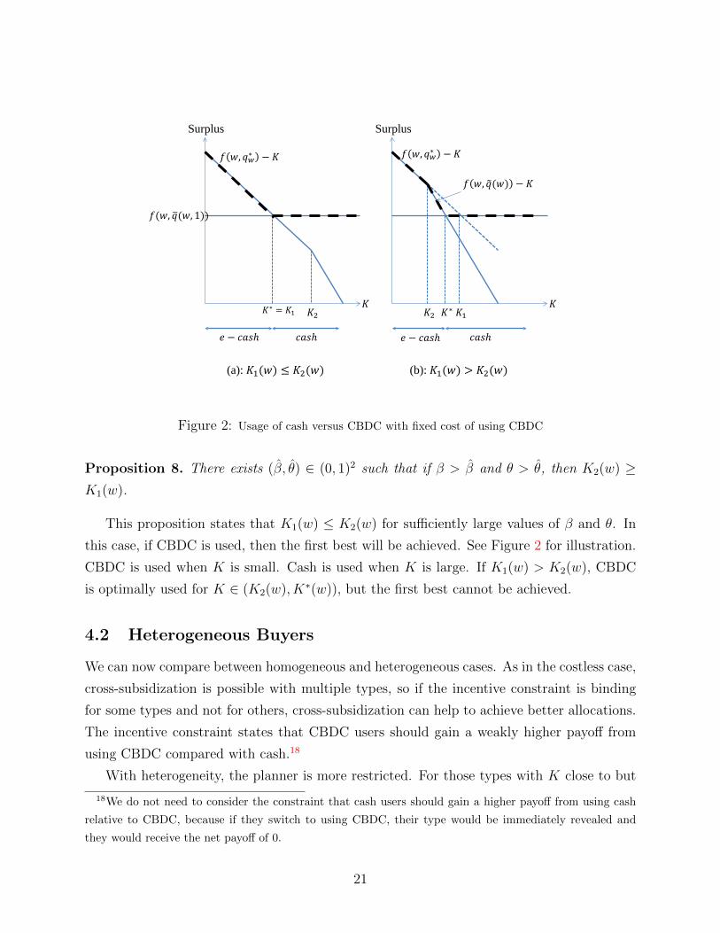
𝐾∗ = 𝐾1 𝐾2

𝑓(𝑤, 𝑞�(𝑤, 1))

𝑓 𝑤, 𝑞𝑤∗ − 𝐾

𝐾

𝑒 − 𝑐𝑐𝑐ℎ 𝑐𝑐𝑐ℎ

𝐾1 𝐾2 𝐾

𝑒 − 𝑐𝑐𝑐ℎ 𝑐𝑐𝑐ℎ

𝐾∗

(a): 𝐾1(𝑤) ≤ 𝐾2(𝑤) (b): 𝐾1(𝑤) > 𝐾2(𝑤)

Surplus Surplus

𝑓 𝑤, 𝑞𝑤∗ − 𝐾

𝑓 𝑤, 𝑞�(𝑤) − 𝐾

Figure 2: Usage of cash versus CBDC with fixed cost of using CBDC

Proposition 8. There exists (β, θ) ∈ (0, 1)2 such that if β > β and θ > θ, then K2(w) ≥K1(w).

This proposition states that K1(w) ≤ K2(w) for sufficiently large values of β and θ. In

this case, if CBDC is used, then the first best will be achieved. See Figure 2 for illustration.

CBDC is used when K is small. Cash is used when K is large. If K1(w) > K2(w), CBDC

is optimally used for K ∈ (K2(w), K∗(w)), but the first best cannot be achieved.

4.2 Heterogeneous Buyers

We can now compare between homogeneous and heterogeneous cases. As in the costless case,

cross-subsidization is possible with multiple types, so if the incentive constraint is binding

for some types and not for others, cross-subsidization can help to achieve better allocations.

The incentive constraint states that CBDC users should gain a weakly higher payoff from

using CBDC compared with cash.18

With heterogeneity, the planner is more restricted. For those types with K close to but

18We do not need to consider the constraint that cash users should gain a higher payoff from using cash

relative to CBDC, because if they switch to using CBDC, their type would be immediately revealed and

they would receive the net payoff of 0.

21

less than K∗(w), use of CBDC is optimal when the population is homogeneously composed

of w, because the cash inflation can be set very high. However, if there is a sufficiently high

measure of agents who want to use cash, then setting a high cash inflation rate amounts to

a significant loss in social welfare, because it affects all cash users. As a result, cash inflation

cannot be too high. Therefore, such a type w may switch to cash (inefficiently compared

with the homogeneous case) because the punishment for using cash cannot be severe enough

to induce him to use CBDC.

4.2.1 Cash Is Used in Small-Value Transactions

In the following result, we establish that when co-existence is optimal, low-type buyers use

cash and high-type buyers use CBDC. That is, cash is used for small-value transactions and

CBDC is used for large-value transactions under the optimal policy. Define:

Q(r) ≡ arg maxq{ru(q)− c(q)}.

Proposition 9. Assume rQ′′(r)Q′(r)

≥ −1. Then there exists a threshold wt > 0 such that agents

with w < wt use cash and agents with w ≥ wt use CBDC under the optimal policy.

The only requirement of this result is that the coefficient of relative risk aversion of Q

should be less than 1. This result is not trivial. Cash inflation is not ∞, so some agents can

receive a strictly positive payoff by using cash. Since the size of the surplus is higher for higher

types, they receive a higher payoff for a given cash inflation. If their payoff from holding

cash increases very fast with their type, it may not be worth it for the planner to have these

types use CBDC. It is shown that if rQ′′(r)Q′(r)

≥ −1, this does not happen.19 This condition is

satisfied for the production and cost functions, u and c, usually used in economics. As an

example, let u(q) = q1−1/c0 with c0 > 1 and c(q) = c1q. Hence, Q(r) = ( (1−1/c0)c1

)c0rc0 , sorQ′′(r)Q′(r)

= c0(c0 − 1)/c0 = c0 − 1 > 0 ≥ −1.20

19This finding is consistent with facts from a survey in Canada reported by Fung et al. (2015) that cash is

used mainly for small-value transactions. They add that the share of cash usage relative to the usage of other

means of payment has decreased. Interestingly, they report that the respondents to the survey attribute

their cash usage mostly to its lower cost relative to other means of payment. Other factors, such as security

concerns, acceptance by the merchants, and ease of use, come after the cost.20More generally, consider a constant relative risk averse Q(r) in which − rQ′′(r)

Q′(r) = 1 − c0 where c0 ≥ 0.

This implies that Q(r) = k1rc0 + k0. Therefore, if c and u are such that c′(q)

u′(q) = ( q−k0

k1)1/c0 for some k0, k1

and c0, then the required condition is satisfied.

22

5 Co-Existence of Cash and CBDC in a Two-Type Ex-

ample

I focus in this section on the two-type example. Studying this case, as opposed to many types

or a continuum of types, is relatively easy and captures the main tradeoff. Suppose there are

two types w1 and w2 with K∗(w1) < K < K∗(w2). If the population is homogeneous, type

w1 uses cash and type w2 uses CBDC under the optimal policy. What should the planner

do when there is more than one type and the optimal means of payment for some of them

is different from others? Denote the measure of type w2 buyers by π2 ≡ π and measure of

type w1 buyers by π1 ≡ 1 − π. When all buyers are of type w2, the planner could increase

cash inflation so that no buyer uses cash. In contrast, when all the buyers are of type w1,

the planner has to use cash for w1 and set the cash inflation rate to the lowest possible level,

γc = 1.

Denote by E the optimal welfare level if both types use CBDC, denote by C the optimal

welfare level if both types use cash, and finally denote by B the welfare level if only w1 uses

cash:

E = (1− π2)βσf(w1, q∗1) + π2βσf(w2, q

∗2)−K,

C = (1− π2)βσf(w1, q1(1)) + π2βσf(w2, q2(1)),

B = (1− π2)βσf(w1, q1(γc)) + π2βσf(w2, q2)− π2K.

We know from the results in the previous section that it is not optimal that only type w2 use

cash. Therefore, the planner’s problem can be written as max{E,C,B} where B denotes

the optimal welfare level if only w1 uses cash, and it is obtained from:

B ≡ maxtc,te2,zc1,ze2,γc,γe,q2

B

s.t. tc + π2(te2 − (γe − 1)ze2) = (1− π2)(γc − 1)zc1 (equivalent to (8)),

tc + te2 + ze2 = max{Dw2(q∗w2), Dw2(q2)} (w2’s payment when using CBDC),

tc + zc1 = max{Dw1(q∗w1), Dw1(q1)} (w1’s payment when using cash),

O(w2, γc) ≤ −(γe−β)(te2+ze2)−(γc−β)tc+βσθ(w2u(q2)−c(q2))−K+γete2(incentive constraint).

I assume that β and θ are sufficiently large that q(w) = q∗w under CBDC (according to Propo-

sition 8). Agents do not want to bring more balances than the number of balances needed to

buy the first-best level of production. The incentive constraint for the maximization problem

can then be simplified to:

maxq{−(γc − β)Dw2(q) + βσθ(w2u(q)− c(q))}

23

≤ −(1−β)Dw2(q2)+βσθ(w2u(q2)−c(q2))−K+(1−π2)/π2(γc−1)Dw1(q1)−γctc/π2. (17)

See the appendix for the derivation. A positive tc makes the constraint only tighter. Since tc

does not appear in the objective function, it is optimal to set it to the lowest possible value;

i.e., tc = 0. Now, we obtain the following result.

Proposition 10 (Optimality of positive inflation). Suppose K > 0. In any equilibrium in

which both means of payment are used, the cash inflation rate must be strictly positive; i.e.,

γc > 1.

If γc ≤ 1, then cash should be withdrawn from the CM, requiring CBDC to be injected

into the CM using OMO. These CBDC balances should be financed from CBDC users.

Moreover, as shown earlier, there is an opportunity cost of using CBDC, as the transfers

made to buyers can be used to purchase the DM good only in the next period. This is as

if the inflation for CBDC cannot be less than 1. Finally, CBDC users should incur cost K.

Altogether, if γc ≤ 1, then CBDC is a strictly dominated choice of payment for buyers, so

co-existence is not possible. Finally, note that this result implies that when co-existence is

optimal, the cash inflation must be strictly positive, although it is feasible to run a negative

cash inflation rate.

5.1 Sufficient Conditions for Non-Optimality of Co-Existence

Assumption 2 (Condition for Non-Optimality of Co-Existence). Assume γ0 < γ1, where

γ0 and γ1 are implicitly defined by the following equations:

βσf(w1, q(w1, γ0)) ≡ βσf(w1, q∗1)−K,

maxq{−(γ1−β)Dw2(q)+βσθ(w2u(q)−c(q))} ≡ −(1−β)Dw2(q

∗2)+βσθ(w2u(q∗2)−c(q∗2))−K.

Proposition 11 (Non-Optimality of Co-Existence). Suppose buyers are of only two types:

w1 with probability 1 − π and w2 with probability π. Under Assumption 2, the co-existence

is not optimal if π is sufficiently close to 1.

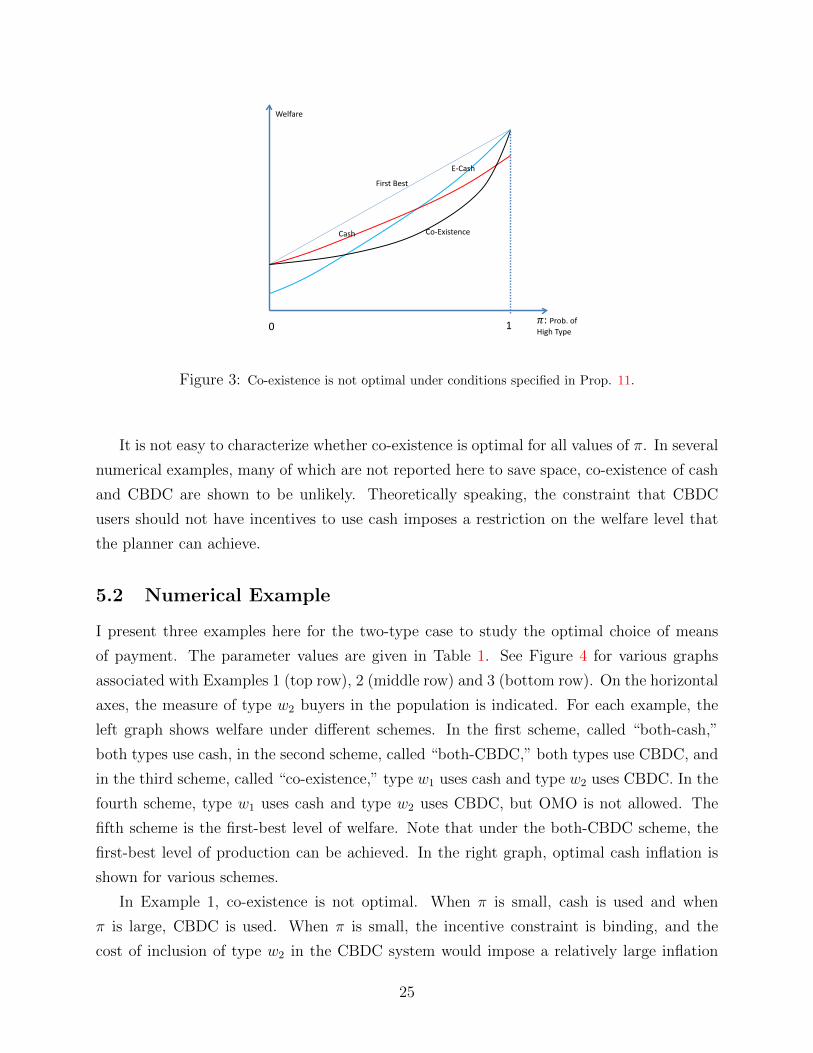
The schematic diagram for this result can be found in Figure 3. A similar result can be

obtained if π is close to 0. It is evident that when π is close to 1, the welfare level under

co-existence is lower than that under the scheme in which both types use CBDC, which is

in turn lower than that under the first best (i.e., the weighted average of the welfare level

under the optimal scheme for each type).

24

First Best

Co-Existence

E-Cash

Cash

Welfare

𝜋: Prob. of High Type 1 0

Figure 3: Co-existence is not optimal under conditions specified in Prop. 11.

It is not easy to characterize whether co-existence is optimal for all values of π. In several

numerical examples, many of which are not reported here to save space, co-existence of cash

and CBDC are shown to be unlikely. Theoretically speaking, the constraint that CBDC

users should not have incentives to use cash imposes a restriction on the welfare level that

the planner can achieve.

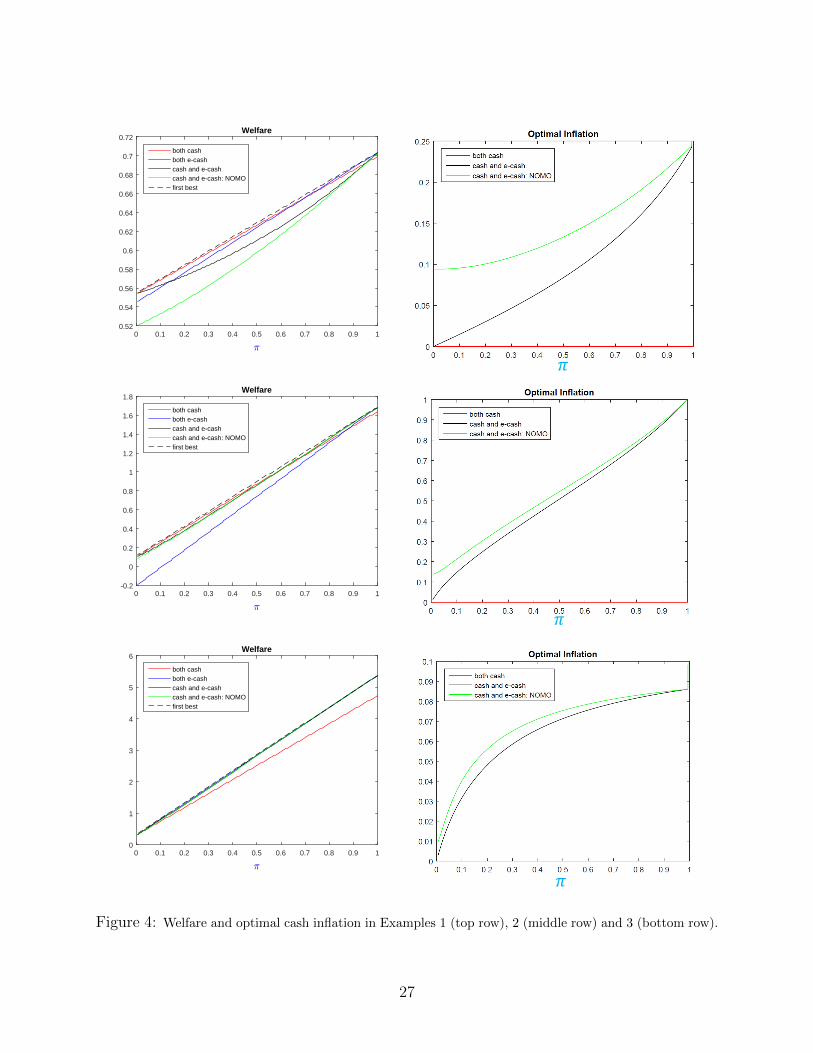
5.2 Numerical Example

I present three examples here for the two-type case to study the optimal choice of means

of payment. The parameter values are given in Table 1. See Figure 4 for various graphs

associated with Examples 1 (top row), 2 (middle row) and 3 (bottom row). On the horizontal

axes, the measure of type w2 buyers in the population is indicated. For each example, the

left graph shows welfare under different schemes. In the first scheme, called “both-cash,”

both types use cash, in the second scheme, called “both-CBDC,” both types use CBDC, and

in the third scheme, called “co-existence,” type w1 uses cash and type w2 uses CBDC. In the

fourth scheme, type w1 uses cash and type w2 uses CBDC, but OMO is not allowed. The

fifth scheme is the first-best level of welfare. Note that under the both-CBDC scheme, the

first-best level of production can be achieved. In the right graph, optimal cash inflation is

shown for various schemes.

In Example 1, co-existence is not optimal. When π is small, cash is used and when

π is large, CBDC is used. When π is small, the incentive constraint is binding, and the

cost of inclusion of type w2 in the CBDC system would impose a relatively large inflation

25

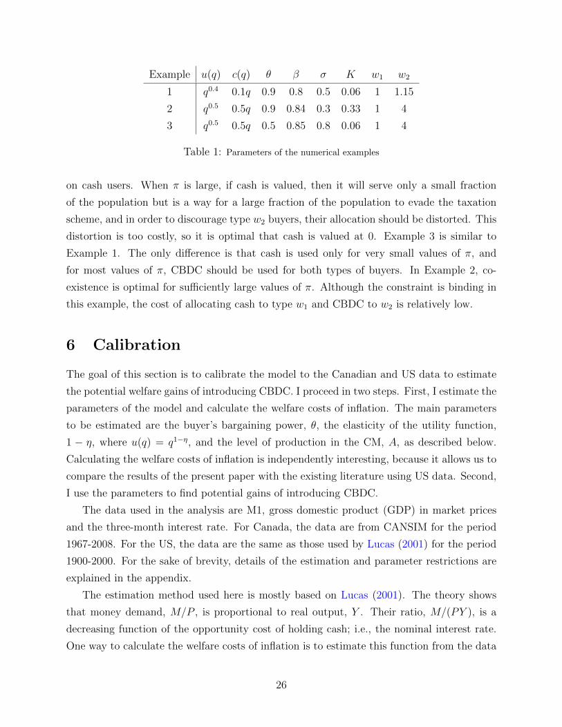
Example u(q) c(q) θ β σ K w1 w2

1 q0.4 0.1q 0.9 0.8 0.5 0.06 1 1.15

2 q0.5 0.5q 0.9 0.84 0.3 0.33 1 4

3 q0.5 0.5q 0.5 0.85 0.8 0.06 1 4

Table 1: Parameters of the numerical examples

on cash users. When π is large, if cash is valued, then it will serve only a small fraction

of the population but is a way for a large fraction of the population to evade the taxation

scheme, and in order to discourage type w2 buyers, their allocation should be distorted. This

distortion is too costly, so it is optimal that cash is valued at 0. Example 3 is similar to

Example 1. The only difference is that cash is used only for very small values of π, and

for most values of π, CBDC should be used for both types of buyers. In Example 2, co-

existence is optimal for sufficiently large values of π. Although the constraint is binding in

this example, the cost of allocating cash to type w1 and CBDC to w2 is relatively low.

6 Calibration

The goal of this section is to calibrate the model to the Canadian and US data to estimate

the potential welfare gains of introducing CBDC. I proceed in two steps. First, I estimate the

parameters of the model and calculate the welfare costs of inflation. The main parameters

to be estimated are the buyer’s bargaining power, θ, the elasticity of the utility function,

1 − η, where u(q) = q1−η, and the level of production in the CM, A, as described below.

Calculating the welfare costs of inflation is independently interesting, because it allows us to

compare the results of the present paper with the existing literature using US data. Second,

I use the parameters to find potential gains of introducing CBDC.

The data used in the analysis are M1, gross domestic product (GDP) in market prices

and the three-month interest rate. For Canada, the data are from CANSIM for the period

1967-2008. For the US, the data are the same as those used by Lucas (2001) for the period

1900-2000. For the sake of brevity, details of the estimation and parameter restrictions are

explained in the appendix.

The estimation method used here is mostly based on Lucas (2001). The theory shows

that money demand, M/P , is proportional to real output, Y . Their ratio, M/(PY ), is a

decreasing function of the opportunity cost of holding cash; i.e., the nominal interest rate.

One way to calculate the welfare costs of inflation is to estimate this function from the data

26

:

0 0.1 0.2 0.3 0.4 0.5 0.6 0.7 0.8 0.9 10.52

0.54

0.56

0.58

0.6

0.62

0.64

0.66

0.68

0.7

0.72Welfare

both cashboth e-cashcash and e-cashcash and e-cash: NOMOfirst best

𝜋

:

0 0.1 0.2 0.3 0.4 0.5 0.6 0.7 0.8 0.9 1-0.2

0

0.2

0.4

0.6

0.8

1

1.2

1.4

1.6

1.8Welfare

both cashboth e-cashcash and e-cashcash and e-cash: NOMOfirst best

𝜋

:

0 0.1 0.2 0.3 0.4 0.5 0.6 0.7 0.8 0.9 10

1

2

3

4

5

6Welfare

both cashboth e-cashcash and e-cashcash and e-cash: NOMOfirst best

𝜋

Figure 4: Welfare and optimal cash inflation in Examples 1 (top row), 2 (middle row) and 3 (bottom row).

27

by finding the best fit, then calculate the area under the demand curve from the inflation

level of π0 to π0 + 0.10 to estimate the welfare costs of 10% inflation. Another way is to

have a model that generates a money demand function. One should then try to find the

parameters of the model such that the money demand function generated by the model fits

the data as much as possible. Finally, one can calculate the welfare costs of inflation implied

by the model. Many papers, including Lucas (2001), Lagos and Wright (2005) and Craig

and Rocheteau (2008), also use the latter approach to estimate welfare costs of inflation for

the US data. I follow this methodology.

In the first step, I estimate parameters (θ, η, A), taking as given the discount factor, β,

and the probability of matching in the DM, σ. Throughout this section, I set β = 0.97; that

is, the real interest rate is set to 3%. I assume that c(q) = q; that is, the cost of producing

q units of the DM good for sellers is q. In the benchmark exercise, I set σ = 0.5, although

I estimate parameters assuming other values for σ as well.21 For estimating parameters, I

assume agents are homogeneous; i.e., w1 = w2.22 For the results to be comparable with

the aforementioned papers, I normalize w1 = 1/(1 − η); that is, the buyer’s utility from

consuming q units of the DM good is q1−η/(1 − η). With a linear production function in

the CM, the level of production in equilibrium is indeterminate. Following the literature, I

assume the production function in the CM is U(X) = A ln(X). This implies that the level

of production in the CM is X∗ = A.

I estimate (θ, η, A) by minimizing the distance between the data and the model-generated

real balances–income ratio, M/(PY ), subject to the constraint that the markup (price over

marginal cost minus 1) in the DM is µ = 10% under the 2% inflation rate in the benchmark

estimation.23 Fixing the markup imposes a constraint on variables. The difference between

my approach and that typically used in the literature is that I place this constraint explic-

itly in the minimization problem. In the estimation, I assume that only cash is available.

Since I use M1 to represent cash, and most elements of M1 are not interest bearing, this

assumption is consistent with the main presumption of the model that cash is not interest

bearing. Introducing CBDC, then, is equivalent to introducing interest-bearing money into

21In the estimation, I fix σ. If I include σ in the optimization parameters, the estimates of welfare costs

of inflation do not change substantially, but the estimates of parameters (θ, η) would be very sensitive, in

that various pairs of (θ, η) lead to almost the same fit. Yet, I conduct various robustness checks depicted in

Tables 2 and 3.22In some exercises not reported here, I estimate the model allowing w2 to be different from w1, but w2 is

not identified, in that various combinations of parameters yield to almost the same fit.23For the robustness check, I consider µ = 20%. Also, I consider the average markup of both DM and CM

and estimate parameters, with this average markup being 10%.

28

the economy.

The estimates for Canada and the US are reported in Tables 2 and 3, respectively. The

benchmark estimates are shown in the top row of the tables in bold. The ratio of real

balances to income is plotted against the nominal interest rate for both data points and

model-generated points based on the benchmark estimates in Figures 5 and 7 for Canada

and the US, respectively. The welfare costs of inflation based on the benchmark estimates

are shown in Figures 6 and 8. Following Lagos and Wright (2005), the welfare costs of a

given level of inflation are calculated as the fraction of consumption that agents are willing

to forgo to be in equilibrium with a 0 inflation rate (or 3% interest rate).

The welfare cost of 10% inflation in the benchmark estimation is 0.96% for Canada and

1.88% for the US. The range of welfare costs for different parameter values is from 0.8%

to 2.8% for Canada and 1.19% to 5.81% for the US. My estimates of welfare costs of 10%

inflation for the US are close to estimates in the literature. Lagos and Wright (2005) estimate

these welfare costs as ranging from 1% to 5% and Craig and Rocheteau (2008) estimate these

costs as ranging from 0.5% to 5%. Also, the lower bound in my estimates is close to the

upper bound in the estimate of Lucas (2001) (less than 1%).

In the second part, I estimate the welfare gains of introducing CBDC into the economy.

This estimate crucially depends on the choice of K, the cost of using CBDC relative to cash

in a transaction. I calculate a range for possible gains of introducing CBDC when the cost

of using CBDC in transactions relative to cash ranges from 0% to 0.5% of the transaction

value. The welfare gains of introducing CBDC are calculated relative to 0% inflation. That

is, I calculate the welfare at 0% inflation when only cash is used, and then compare it with

the optimal level of welfare when CBDC can be used too. More precisely, I calculate the level

of additional consumption that makes the agents indifferent between being in equilibrium

with 0% inflation with only cash circulated in the economy, and being in equilibrium under

the optimal policy with both cash and CBDC.

Results regarding the welfare gains of introducing CBDC are summarized in Tables 4 and

5 for Canada and the US, respectively.24 The benchmark estimations are depicted in the top

rows of the tables. When the cost of using CBDC relative to cash is 0%, the welfare gains

of introducing CBDC are 0.11% for Canada and 0.26% for the US. With other parameter

specifications, the welfare gains range from 0.11% to 64% for Canada and from 0.15% to

1.6% for the US.

I also allow buyers to be homogeneous (w1 = w2) or heterogeneous (w2 < w1). When w2

24The optimal scheme requires co-existence when only w2 uses CBDC. See the last column of Tables 4

and 5.

29

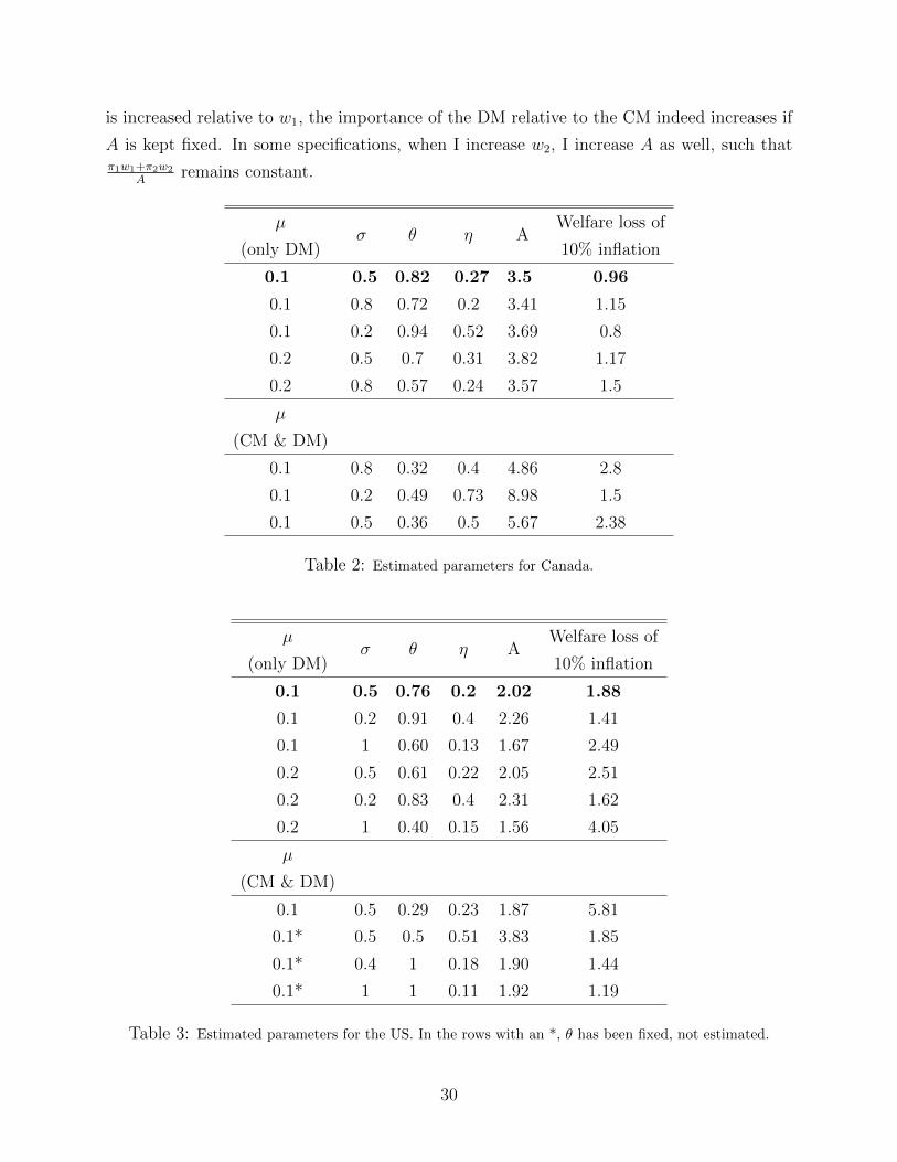
is increased relative to w1, the importance of the DM relative to the CM indeed increases if

A is kept fixed. In some specifications, when I increase w2, I increase A as well, such thatπ1w1+π2w2

Aremains constant.

µ

(only DM)σ θ η A

Welfare loss of

10% inflation

0.1 0.5 0.82 0.27 3.5 0.96

0.1 0.8 0.72 0.2 3.41 1.15

0.1 0.2 0.94 0.52 3.69 0.8

0.2 0.5 0.7 0.31 3.82 1.17

0.2 0.8 0.57 0.24 3.57 1.5

µ

(CM & DM)

0.1 0.8 0.32 0.4 4.86 2.8

0.1 0.2 0.49 0.73 8.98 1.5

0.1 0.5 0.36 0.5 5.67 2.38

Table 2: Estimated parameters for Canada.

µ

(only DM)σ θ η A

Welfare loss of

10% inflation

0.1 0.5 0.76 0.2 2.02 1.88

0.1 0.2 0.91 0.4 2.26 1.41

0.1 1 0.60 0.13 1.67 2.49

0.2 0.5 0.61 0.22 2.05 2.51

0.2 0.2 0.83 0.4 2.31 1.62

0.2 1 0.40 0.15 1.56 4.05

µ

(CM & DM)

0.1 0.5 0.29 0.23 1.87 5.81

0.1* 0.5 0.5 0.51 3.83 1.85

0.1* 0.4 1 0.18 1.90 1.44

0.1* 1 1 0.11 1.92 1.19

Table 3: Estimated parameters for the US. In the rows with an *, θ has been fixed, not estimated.

30

interest rate (%)2 4 6 8 10 12 14 16 18

real

bal

ance

s--in

com

e ra

tio

0.06

0.08

0.1

0.12

0.14

0.16

0.18

0.2

0.22

0.24

0.26Data and model

Figure 5: Data and model for Canada

interest rate (%)2 4 6 8 10 12 14 16 18

cons

umpt

ion

loss

rel

ativ

e to

zer

o in

flatio

n (%

)

-0.2

0

0.2

0.4

0.6

0.8

1

1.2

1.4

1.6Cost of inflation

Figure 6: Welfare cost of inflation for Canada

31

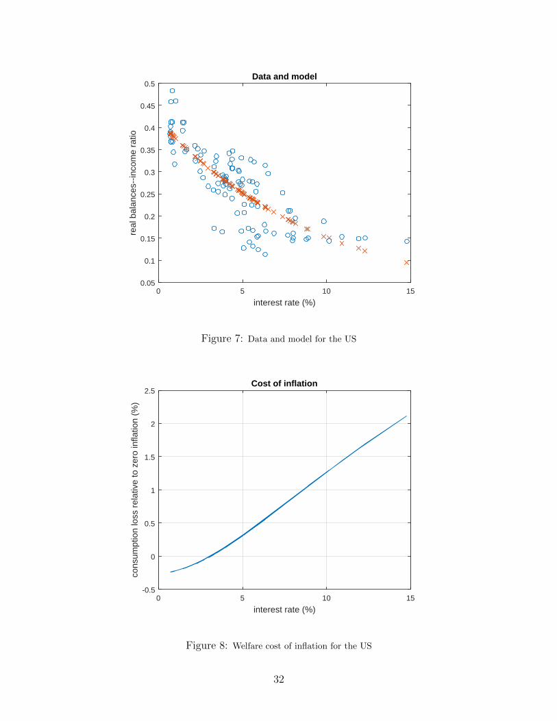
interest rate (%)0 5 10 15

real

bal

ance

s--in

com

e ra

tio

0.05

0.1

0.15

0.2

0.25

0.3

0.35

0.4

0.45

0.5Data and model

Figure 7: Data and model for the US

interest rate (%)0 5 10 15

cons

umpt

ion

loss

rel

ativ

e to

zer

o in

flatio

n (%

)

-0.5

0

0.5

1

1.5

2

2.5Cost of inflation

Figure 8: Welfare cost of inflation for the US

32

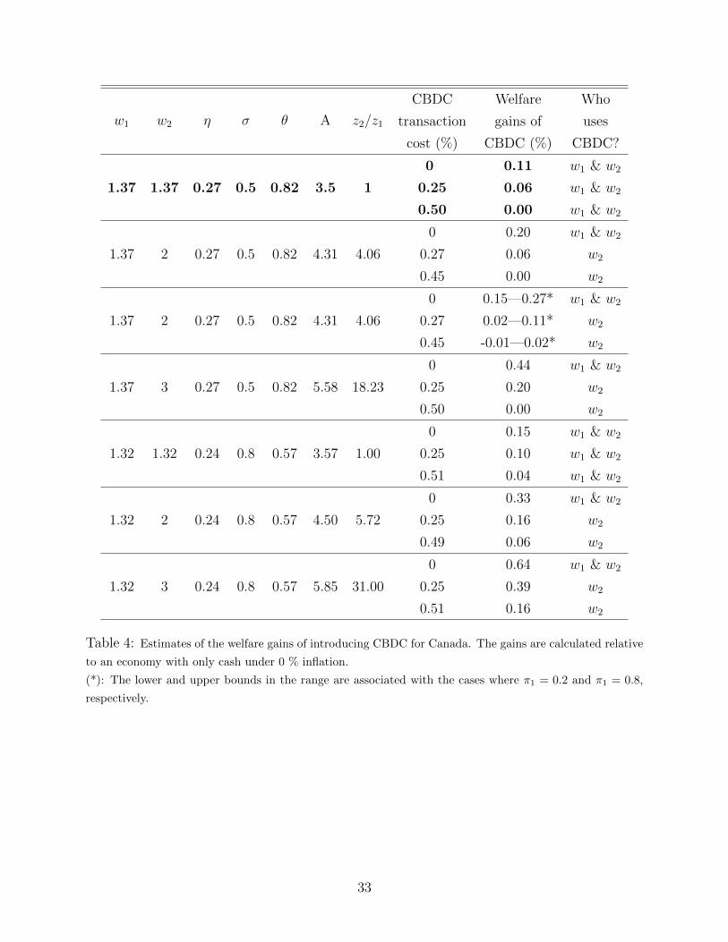
w1 w2 η σ θ A z2/z1

CBDC

transaction

cost (%)

Welfare

gains of

CBDC (%)

Who

uses

CBDC?

0 0.11 w1 & w2

1.37 1.37 0.27 0.5 0.82 3.5 1 0.25 0.06 w1 & w2

0.50 0.00 w1 & w2

0 0.20 w1 & w2

1.37 2 0.27 0.5 0.82 4.31 4.06 0.27 0.06 w2

0.45 0.00 w2

0 0.15—0.27* w1 & w2

1.37 2 0.27 0.5 0.82 4.31 4.06 0.27 0.02—0.11* w2

0.45 -0.01—0.02* w2

0 0.44 w1 & w2

1.37 3 0.27 0.5 0.82 5.58 18.23 0.25 0.20 w2

0.50 0.00 w2

0 0.15 w1 & w2

1.32 1.32 0.24 0.8 0.57 3.57 1.00 0.25 0.10 w1 & w2

0.51 0.04 w1 & w2

0 0.33 w1 & w2

1.32 2 0.24 0.8 0.57 4.50 5.72 0.25 0.16 w2

0.49 0.06 w2

0 0.64 w1 & w2

1.32 3 0.24 0.8 0.57 5.85 31.00 0.25 0.39 w2

0.51 0.16 w2

Table 4: Estimates of the welfare gains of introducing CBDC for Canada. The gains are calculated relative

to an economy with only cash under 0 % inflation.

(*): The lower and upper bounds in the range are associated with the cases where π1 = 0.2 and π1 = 0.8,

respectively.

33

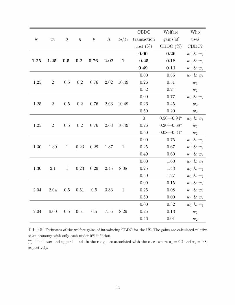
w1 w2 σ η θ A z2/z1

CBDC

transaction

cost (%)

Welfare

gains of

CBDC (%)

Who

uses

CBDC?

0.00 0.26 w1 & w2

1.25 1.25 0.5 0.2 0.76 2.02 1 0.25 0.18 w1 & w2

0.49 0.11 w1 & w2

0.00 0.86 w1 & w2

1.25 2 0.5 0.2 0.76 2.02 10.49 0.26 0.51 w2

0.52 0.24 w2

0.00 0.77 w1 & w2

1.25 2 0.5 0.2 0.76 2.63 10.49 0.26 0.45 w2

0.50 0.20 w2

0 0.50—0.94* w1 & w2

1.25 2 0.5 0.2 0.76 2.63 10.49 0.26 0.20—0.68* w2

0.50 0.08—0.34* w2

0.00 0.75 w1 & w2

1.30 1.30 1 0.23 0.29 1.87 1 0.25 0.67 w1 & w2

0.49 0.60 w1 & w2

0.00 1.60 w1 & w2

1.30 2.1 1 0.23 0.29 2.45 8.08 0.25 1.43 w1 & w2

0.50 1.27 w1 & w2

0.00 0.15 w1 & w2

2.04 2.04 0.5 0.51 0.5 3.83 1 0.25 0.08 w1 & w2

0.50 0.00 w1 & w2

0.00 0.32 w1 & w2

2.04 6.00 0.5 0.51 0.5 7.55 8.29 0.25 0.13 w2

0.46 0.01 w2

Table 5: Estimates of the welfare gains of introducing CBDC for the US. The gains are calculated relative

to an economy with only cash under 0% inflation.

(*): The lower and upper bounds in the range are associated with the cases where π1 = 0.2 and π1 = 0.8,

respectively.

34

7 Extension

I assume in this section that there is no direct cost of carrying CBDC—i.e., K = 0—but

CBDC cannot be used in a fraction of transactions. For example, the seller may not be able to

accept CBDC because no internet or electricity connection is available, or because the seller

does not have access to CBDC technology (such as un-banked agents in remote locations).

Another reason might be that the buyers do not want to use CBDC in some transactions

so that they can keep their anonymity. Formally, assume that in αc ∈ [0, 1] fraction of

transactions, only cash can be used (c-meetings); in αe ∈ [0, 1] fraction of transactions, only

CBDC can be used (e-meetings); and in αb ∈ [0, 1] fraction of transactions, both cash and

CBDC can be used (b-meetings).25 Of course, αc + αe + αb ≤ 1.26 Note that the buyers

learn the type of the meeting only after they match with a seller. Therefore, and in contrast

to the previous sections, a given agent may want to hold both means of payment as they do

not know which means of payment can be used in the DM. The case of αc = 0 is similar to

the benchmark model in the previous sections with K = 0, in that using CBDC is costless,

so cash is redundant. In the case of αc > 0, CBDC users may effectively incur a cost for

using CBDC, as their means of payment cannot be used in some transactions.

I assume without loss of generality that the planner is not allowed to make cash transfers,

i.e., tc = 0.27 Furthermore, I do not study the heterogeneity of types in this section; type w

is fixed and the same for all buyers.28 Therefore, the index w is removed from the notation.

The rest of the environment is exactly the same as in the benchmark model. In particular,

I continue to assume that the transfer to agents, whether in cash or CBDC form, cannot be

negative. That is, the planner does not have the power of taxation.

For a given policy, the agent’s problem is given as follows:

maxzc,ze

{− (γc − β)zc − (γe − β)ze + βte(ze) + βσθ

(αcf(qc) + αef(qe) + αbf(qb)

)}(18)

25In making this assumption, I follow Rocheteau et al. (2014) and Zhu and Hendry (2017). In the former,

fiat money and bond, and in the latter, money and private e-money are means of payment.26Especially when doing comparative statics, I allow their sum to be less than 1. The interpretation is

that in some transactions, the buyer and seller may not trade with any means of payment.27To show this claim, start from an allocation with a strictly positive tc. Change tc to 0 but conduct

OMO such that the same amount of cash is injected into the economy in exchange for CBDC. Next, transfer

CBDC to the agents (and possibly adjust the CBDC inflation) so that the DM production levels in all three

types of meetings remain the same.28I had heterogeneity in the benchmark model to generate demand for both means of payment endoge-

nously. In this section, since one means of payment may not be useful in some transactions, agents may

want to bring both means of payment from the CM. Therefore, I do not need to have heterogeneity of types

anymore.

35

where

qc = min{q∗, D−1(zc)}, (19)

qe = min{q∗, D−1(ze + te)}, (20)

qb = min{q∗, D−1(zc + ze + te)}. (21)

The planner’s problem is to choose a policy that maximizes welfare, and can be written as

follows:

maxzc,ze,te(.),γc,γe

{αcf(qc) + αef(qe) + αbf(qb)}

s.t. te(ze) = (γc − 1)zc + (γe − 1)ze, (22)

where (qc, qe, qb) is obtained from the agent’s maximization problem given above.

Since the punishment in the case that the agent does not bring enough CBDC balances is

severe (i.e., receiving no transfers), we can assume without loss of generality that if an agent

brings CBDC, then the agent will bring the exact amount of CBDC that the planner wants.

Similar to the benchmark model, to support this punishment, the inflation rate for CBDC

should be sufficiently high that the CBDC transfers for agents who bring enough balances

become positive. Therefore, the only relevant constraint is that agents should not gain if

they bring all their portfolio in the form of cash. This constraint is summarized by:

maxzc

{− (γc − β)zc + βσθ

(αcf(qc) + αbf(qb)

)}− (γe − β)ze + βte(ze) + βσθαef(qe)

≥ maxq

{− (γc − β)D(q) + βσθ(αc + αb)f(q)

}. (23)

Also, define

zc ∈ arg maxz′c

{−(γc−β)z′c+βσθ

(αcf(min{q∗, D−1(z′c)})+αbf(min{q∗, D−1(z′c+ze+te)})

)}.

(24)

From now on, I summarize the optimal policy by zc and qb. From (19), zc pins down qc. One

then obtains γc from (24) consistent with zc, qb and qc, and ze and te from (21) and (22) for

a given γe. Finally, qe is given by (20).

7.1 Sufficient Conditions to Achieve the First Best

Remember that in Section 3, the first-best level of welfare cannot be attained when K > 0,

because even if β and θ are sufficiently high, the buyers still have to incur the direct cost of

carrying CBDC. Here, in contrast, the first-best level of welfare can be achieved if β and θ

are sufficiently high even when αc > 0. To achieve the first best, the planner runs deflation

36

on cash at the rate of time preferences—i.e., γc = β—and then runs inflation on CBDC to

finance the deflation by withdrawing cash and injecting CBDC in the CM through OMO.

OMO is crucial for this result. Also, similar to the transfer scheme used previously, the

planner makes CBDC transfers to agents only if they bring enough CBDC balances from the

CM. If they do not, then the planner does not give them the subsidy.

Proposition 12. Assume αc = 0. Then the first best is achievable if and only if:

βσ(αe + αb)θ(wu(q∗)− c(q∗)) ≥ (1− β)D(q∗). (25)

Now assume that αc > 0. Then the first best is achievable if:

βσαeθ(wu(q∗)− c(q∗)) ≥ 2(1− β)D(q∗). (26)

Some points are worth mentioning. If αc = 0, the condition needed to achieve the first

best is equivalent to that in Proposition 3. In the general case of αc > 0, to achieve the first

best, the planner needs to ensure that buyers have enough balances in all types of meetings

to achieve the first best. Regarding the c-meetings, the planner needs to run a cash growth

rate equal to the discount factor to reduce the cost of holding real balances to 0. Regarding

the e-meetings, the planner simply needs to ensure that the number of balances in CBDC

that the agents carry, together with what they receive as transfers, is enough to buy the

first-best level of production. The planner would not worry about the b-meetings because

agents have enough balances to buy the first-best level of consumption by using only one

means of payment.

7.2 Optimal Scheme When the First Best Cannot Be Achieved

Now assume that the first best is achievable when there are no c-meetings—i.e., when

αc = 0—but it is not achievable otherwise. That is, (25) holds but (26) does not. We

are interested in knowing whether both means of payment are valued in the optimal alloca-

tion (co-existence) or only one means of payment is valued. Particularly, how is the use of

means of payment changed when αc increases from 0? Do buyers choose to bring a small

amount of cash from the CM? Or, is there a threshold for αc below which they do not use

cash even though cash is useful in some meetings?

The tradeoff that the planner faces is similar to that in the benchmark model. If cash

is valued in the equilibrium, then agents can substitute cash for CBDC in the b-meetings.

Therefore, agents have less incentive to bring CBDC. This, in turn, implies that welfare

gains from CBDC, due to its flexibility, are less likely to be realized. If cash is not valued,

there will be no trade in the c-meetings. The optimal policy trades off these two forces.

37

Proposition 13. Suppose αc + αe + αb = 1 and that αc > 0. Assume that (25) holds but

(26) does not. That is, the first best can be achieved when αc = 0 but not when αc > 0. Then

the following results are obtained:

(a) Assume αb = 0. Suppose (25) holds with strict inequality. Then cash is valued in the

optimal allocation.

(b) Assume αe = 0. If both means of payment are valued and the first best cannot be

achieved in any meetings, then cash inflation must be strictly positive.

Part (a) states that when αc > 0, it is optimal to use cash. Notice that this result holds

even without Inada conditions. There are two countervailing forces. When cash is valued,

it is effectively a leeway for agents to evade the taxation policy to which the CBDC users

are subjected. Since there are no b-meetings, the choice of cash is independent of the choice

of CBDC. The planner would have cash circulated as long as there are some meetings for

which cash is useful. Therefore, cash is absolutely essential in this economy. This result is in

contrast to the result in the benchmark model in which under certain conditions cash is not

used in the optimal allocation. Finally, when αc is small, the planner needs to run deflation

to implement this allocation. This means that using OMO (to inject CBDC and withdraw

cash from the CM) is crucial here.

Part (b) simply states that cash inflation is necessary to provide incentive to agents to

hold CBDC. If cash inflation is too low, agents would have incentive to use cash in both

c-meetings and b-meetings, and therefore, the welfare gains associated with using CBDC

would not be realized. This result is similar to the benchmark model.

Proposition 14. (a) Assume αe = 0. There exists αc < 1 such that if αc ≥ αc, then only

cash is valued in the optimal allocation.

(b) Assume αb = 0 and u′(0) < ∞. There exists αc < 1 such that if αc ≥ αc, then only

cash is valued in the optimal allocation.

I summarize the analytical results so far in the space of αc and αe in Figure 9. There are

three schemes for means of payment: cash-only (in which all agents use only cash), CBDC-

only (in which all agents use only CBDC), and both cash and CBDC (in which agents use

both means of payment). Ideally, one would like to identify the regions under which each

scheme is optimal, but analytically it is not easy to do that for the entire space. This is why

I identify the optimal schemes on only some boundaries of the region. On the horizontal

axes, αe is depicted, and on the vertical axes, αc is depicted.

When αc = 0, cash is redundant, and if (25) holds, even the first best is achievable.

If αe = 0, then Proposition 14(a) implies that the cash-only scheme is optimal. Similarly,

38

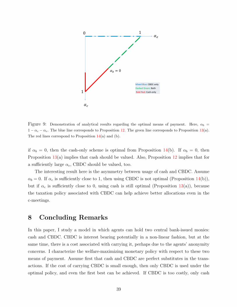
𝛼𝑒

𝛼𝑐

Mixed Blue: CBDC-only Dashed Green: Both Bold Red: Cash-only

0 1

1

𝛼𝑏 = 0

Figure 9: Demonstration of analytical results regarding the optimal means of payment. Here, αb =

1− αc − αe. The blue line corresponds to Proposition 12. The green line corresponds to Proposition 13(a).

The red lines correspond to Proposition 14(a) and (b).

if αb = 0, then the cash-only scheme is optimal from Proposition 14(b). If αb = 0, then

Proposition 13(a) implies that cash should be valued. Also, Proposition 12 implies that for

a sufficiently large αe, CBDC should be valued, too.

The interesting result here is the asymmetry between usage of cash and CBDC. Assume

αb = 0. If αc is sufficiently close to 1, then using CBDC is not optimal (Proposition 14(b)),

but if αc is sufficiently close to 0, using cash is still optimal (Proposition 13(a)), because

the taxation policy associated with CBDC can help achieve better allocations even in the

c-meetings.

8 Concluding Remarks

In this paper, I study a model in which agents can hold two central bank-issued monies:

cash and CBDC. CBDC is interest bearing potentially in a non-linear fashion, but at the

same time, there is a cost associated with carrying it, perhaps due to the agents’ anonymity

concerns. I characterize the welfare-maximizing monetary policy with respect to these two

means of payment. Assume first that cash and CBDC are perfect substitutes in the trans-

actions. If the cost of carrying CBDC is small enough, then only CBDC is used under the

optimal policy, and even the first best can be achieved. If CBDC is too costly, only cash

39

is used. If the cost of carrying CBDC is intermediate, welfare under co-existence may be

dominated by the scheme in which only one means of payment is used. This is because

under co-existence, agents use cash as a way to evade the taxation scheme that CBDC users

are subjected to; therefore, co-existence leads to under-utilization of gains of CBDC rising

from its interest-bearing feature. When cash and CBDC are not perfect substitutes, then

co-existence is more likely to be optimal. Furthermore, CBDC can help achieve better al-

locations even for the meetings in which only cash can be used. This is possible through

OMO, where the planner exchanges cash for CBDC to run the Friedman rule for cash.

A system that can implement the CBDC discussed in this paper is a debit card system

that is owned and monitored by the central bank (although its operations can be outsourced

to other institutions such as “FinTech” companies, if they can do it with low operational

costs). Each individual can have an account with the central bank, and individuals can use

these balances for purchases of goods and services. Such a system provides access to the

central bank balance sheet in electronic format for all agents in the population and allows

them to earn interest on their balances. Currently, only some financial institutions have this

privilege. With such a system, monetary policy directly affects agents’ decisions to carry

balances, rather than through the financial system, making the implementation of monetary

policy more transparent. (See Berentsen and Schar (2018).)

Introducing CBDC would have non-trivial effects on the banking system. If CBDC is

available, it provides direct access for agents to a perfectly safe deposit account. Such an

account would be safer than the deposits at commercial banks (at least for the deposits

exceeding the amount insured by, say, the Canada Deposit Insurance Corporation), so those

agents who want a perfectly safe deposit vehicle do not deposit at commercial banks. There-

fore, CBDC acts as a competitor for bank deposits. On one hand, this elevated level of

competition may lead banks to improve their services by offering cheaper and/or better

products. On the other hand, an increased level of competition may lead banks to invest

in (or give loan to) riskier projects, resulting in a less stable financial system. Furthermore,

banks may increase the interest rate on loans, which in turn can affect the real economy.

The effects of CBDC on the banking system, both in the steady state and also in times of

crisis, are yet to be explored.

40

References

R. Agarwal and M. Kimball. Breaking through the zero lower bound. IMF Working Paper

No. 15/224, 2015.

D. Andolfatto. Essential interest-bearing money. Journal of Economic theory, 145(4):1495–

1507, 2010.

J. Barrdear and M. Kumhof. The macroeconomics of central bank issued digital currencies.

Bank of England Staff Working Paper No. 605, 2016.

M. Bech and R. Garratt. Central bank cryptocurrencies. BIS Quarterly Review, page 55,

2017.

A. Berentsen and F. Schar. The case for central bank electronic money and the non-case for

central bank cryptocurrencies. Federal Reserve Bank of St. Louis Review, Early Edition,

2018.

O. Bjerg. Designing new money-the policy trilemma of central bank digital currency. Copen-

hagen Business School Working Paper, 2017.

J. Chiu and T.-N. Wong. On the essentiality of e-money. Technical report, Bank of Canada

Staff Working Paper, 2015.

J. Chiu, M. Dong, and E. Shao. On the welfare effects of credit arrangements. Bank of

Canada Staff Working Paper 2012-43, 2012.

Committee on Payments and Market Infrastructures. Digital currencies. Bank of Interna-

tional Settlements, November 2015.

B. Craig and G. Rocheteau. Inflation and welfare: A search approach. Federal Reserve Bank

of Cleveland Policy Discussion Paper Number 12, 2006.

B. Craig and G. Rocheteau. Inflation and welfare: A search approach. Journal of Money,

Credit and Banking, 40(1):89–119, 2008.

M. Dong and J. H. Jiang. One or two monies? Journal of Monetary Economics, 57(4):

439–450, 2010.

B. Fung and H. Halaburda. Central bank digital currencies: a framework for assessing why

and how. Bank of Canada Staff Discussion Paper 2016-22, 2016.

41

B. Fung, K. P. Huynh, and G. Stuber. The use of cash in canada. Bank of Canada Review,

2015(Spring):45–56, 2015.

P. Gomis-Porqueras and D. Sanches. Optimal monetary policy in a model of money and

credit. Journal of Money, Credit and Banking, 45(4):701–730, 2013.

C. Gu, F. Mattesini, and R. Wright. Money and credit redux. Econometrica: Journal of the

Econometric Society, 84(1):1–32, 2016.

C. Kahn, F. Rivadeneyra, and T.-N. Wong. E-money and payment policy. Technical report,

Bank of Canada Staff Working Paper, 2017.

R. Lagos and R. Wright. A unified framework for monetary theory and policy analysis.

Journal of Political Economy, 113(3):463–484, 2005.

R. E. Lucas. Inflation and welfare. In Monetary Theory as a Basis for Monetary Policy,

pages 96–142. Springer, 2001.

G. Rocheteau and R. Wright. Money in search equilibrium, in competitive equilibrium, and

in competitive search equilibrium. Econometrica, 73(1):175–202, 2005.

G. Rocheteau, R. Wright, and S. X. Xiao. Open market operations. Technical report, mimeo,

2014.

K. S. Rogoff. The curse of cash. Princeton: Princeton University Press, 2016.

C. Skingsley. Should the riksbank issue e-krona? Speech at FinTech Stockholm, 16 November,

2016.

Sveriges Riksbank. The riksbank’s e-krona project: Report 1. September 2017.

J. Tobin. A case for preserving regulatory distinctions. Challenge, 30(5):10–17, 1987.

Y. Zhu and S. Hendry. A framework for analyzing monetary policy with e-money. Technical

report, Mimeo, 2017.

42

Appendix

In this appendix, I first discuss the relationship between my paper and two closely related

papers. Second, I provide proofs for the results. Finally, I elaborate on the calibration

exercise.

Relation with Chiu and Wong (2015)

My paper is among the first to study the payment choice between cash and CBDC, and

how this choice affects the optimal monetary policy. The only paper with something of a

similar objective is Chiu and Wong (2015). Perhaps the most important difference between

my model and theirs is that the features of cash and CBDC emphasized in my model are

different from theirs. In particular, I do not allow for communication between the planner

and the agents if they use cash. Also, I do not allow for the planner’s direct interventions

in the bilateral meetings. I believe these two features are more realistic regarding cash and

the versions of CBDC typically discussed in policy circles.

To elaborate, the first difference between my paper and theirs is with respect to how cash

transfers are made to agents. In their model, the agents can communicate with the planner

or mechanism designer to report their cash holdings, and the planner proposes an allocation

that can depend on their report in a very general way; i.e., there is no requirement on the

functional form of this dependence. In my model, the ability of the planner to implement

monetary policy around cash is very limited. No communication between cash users and the

planner is allowed, and the only possible form of implementing monetary policy regarding

cash is the helicopter drop; i.e., the number of cash transfers to agents cannot depend on

the agent’s characteristics (such as transaction amount). As a result, the first best is never

achievable with cash in my model. Roughly speaking, the CBDC in my paper is equivalent

to cash, together with some form of communication in their paper.

The second difference is that in my model, the planner cannot intervene in the bilateral

meetings. All interventions in my model are done either in the CM (using OMO) or in the

transfer stage before bilateral meetings occur. In contrast, in their model, the planner has

the power to either restrict access to CBDC balances in the DM or make transfers to the

agents in the DM. Therefore, the set of interventions available to the planner in their paper

is different from my paper.29

29There are other differences between the two papers, too. In my paper, the agents are heterogeneous in

their transaction needs, while agents are homogeneous in their paper. I study the cases under which both

means of payment co-exist and are used by different agents. In their paper, co-existence is not studied.

1

Relation with Gomis-Porqueras and Sanches (2013)

I do not assume that the planner has access to the history of transactions, but the fact

that the planner can see the current CBDC balances somewhat summarizes all available

information for the planner whether the agent has worked in the previous CM or not. In

this sense, CBDC in my model acts like credit, which is the focus of their paper. Unlike in

my benchmark model, the credit is not available in their paper in a fraction of meetings, so

their setting is similar to the setting in Section 7 of my paper. Moreover, they do not have

heterogeneity of buyers; therefore, the endogenous adoption of different means of payment

for different agents does not happen in their equilibrium. Finally, they do not have a policy

choice regarding credit. In contrast, in my model, the policy choice of the planner is to

choose how CBDC transfers should be distributed to the agents to induce them to use the

means of payment that leads to the socially optimal outcome.

Proofs

Proof of Lemma 1. One can write

tc+

∫te(ze(w), w)dF (w) = φ+M+ +ψ+E+−φ+M−ψ+E = φ+(M+ +

ψ+

φ+

E+)−φ+(M+ψ

φE)

= φ+(M+ +ψ+

φ+

E+)− φ+(M +ψ

φE) =

φ+

φ++

φ++M+ − φ+M +ψ+

ψ++

ψ++E+ − ψ+E

= (γc − 1)

∫zc(w)dF (w) + (γe − 1)

∫ze(w)dF (w).

For the first equality, (4) and (5) were used. For the third one, (3) was used for t + 1.

Equations (6) and (7) together with (2) were used for the last equality.

Proof of Proposition 1. Consider problem 2. Take the optimal policy {γc, γe, tc, {te(z, w)}w}and denote the equilibrium allocation by {(q(w), zc(w), ze(w))}w. Consider another policy

in which te(z, w) is replaced with

t′e(z, w) =

te(ze(w), w) z ≥ ze(w)

0 z < ze(w).

It is easy to see that the same equilibrium objects form an equilibrium under this new policy,

because the constraints of the planner’s problem continue to hold. Especially note that type

w buyers do not want to bring CBDC any less than in the equilibrium, as they would get

weakly fewer transfers, and they do not want to bring any more either, as they cannot get

2

any transfers more than te(ze(w), w). Finally, their decision regarding cash does not change

either, as cash payments to them are the same as before.

Proof of Proposition 2. For any optimal policy and the associated equilibrium allocation,

another policy and equilibrium will be constructed in which cash is not used and the welfare

remains the same. Consider problem 2. Take the optimal policy {γc, γe, tc, {te(z, w)}w} and

denote the equilibrium allocation by {(q(w), zc(w), ze(w))}w. Consider another policy with

t′c = 0, M ′0 = M0, E ′0 = E0 inflation rate γ′c, γ

′e, and

t′c = 0, t′e(z, w) =

Dw(q(w))− Dw(q(w))+Λc(w)+Λe(w)γ′e

z ≥ Dw(q(w))+Λc(w)+Λe(w)γ′e

0 otherwise

where

Λc(w) ≡ (γc − 1)(tc + zc(w))− γctc,

Λe(w) ≡ (γe − 1)(te(ze(w), w) + ze(w))− γete(ze(w), w).

Set γ′c sufficiently high such that buyers do not want to bring any balances from the CM.

Then it is easy to check that with this policy, agents will choose the same q(w) as in the

original equilibrium.

To give an idea of how the new policy was constructed, note that the buyer’s payoff can

be written as

−(1− β)(zc + ze(w) + tc + te(ze(w), w)︸ ︷︷ ︸Dw(q)

) + βσθ(wu(q)− c(q))− Λc(w)− Λe(w)

following the first constraint in problem 2. I construct γ′e and t′e(z, w) such that the real post-

transfer balances of buyers remain the same as in the original allocation—i.e., t′e(z′e(w), w) +

z′e(w) = Dw(q(w))—and also their payoff remains the same: −Λc(w) − Λe(w) = −(γ′c −1)(t′c + z′c(w)) + γ′ct

′c −(γ′e − 1)(t′e(.) + z′e(w)) + γ′et

′e(.).

Under this policy, if any buyer wants to carry cash, the buyer gets at most maxq{−(γ′c−β)Dw(q) + βσθ(wu(q)− c(q))}, which is 0 if γ′c is set sufficiently high. If any buyer chooses

to bring balances in CBDC but lower than z′e(w), then the buyer can get no more than his

payoff if he uses cash, in which case his payoff is 0. If he brings z′e(w), then he gets a positive

payoff as in the original equilibrium allocation.

Finally, I show below that the last constraint in the problem is also satisfied.

t′c+

∫ [(t′e(z

′e(w), w)−(γ′c−1)z′c(w)−(γ′e−1)z′e(w))

]dF (w) = −

∫ [Λc(w)+Λe(w)

]dF (w) = 0.

3

For the first equality, the construction of a new policy and a new equilibrium allocation was

used. The second one can be simply derived after some algebra and using the fact that the

corresponding constraint in the original equilibrium must hold.

Proof of Proposition 3. First, assume that the condition holds.

Consider the policy {γc, γe, tc, {te(z, w)}w}, the equilibrium allocation {(q(w), zc(w), ze(w))}w,

and CBDC transfer function te(z, w):

te(z, w) =

(γe−1)Dw(q∗w)

γez ≥ Dw(q∗w)

γe

0 z < ze(w).

tc = 0, γe > 1, and γc > 1 is set sufficiently high that maxq{−(γ − β)Dw(q) + βσθ(wu(q)−c(q))} = 0. Under this policy, no buyer wants to carry any cash, as their payoff would be

0. Moreover, the buyer would take exactly ze(w) = Dw(q∗w)γe

real balances from the CM. The

constraint of the planner’s problem is satisfied by the construction of te.

Second, assume that the first best is achievable. By Proposition 2, cash is not used

without loss of generality, so we can assume that tc = 0. Following the second constraint

of the planner’s problem, one obtains te(z, w) = (γe − 1)ze(w). Since first best is achiev-

able, the balances that the agent takes from the CM plus the transfers that he receives,

ze(w) + te(ze(w), w), must be equal to Dw(q∗w). Therefore, ze(w) = Dw(q∗w)γe

, and consequently,

te(z, w) = (γe − 1)ze(w) = (γe−1)Dw(q∗w)γe

. The buyer must get a positive payoff, so

−(γe − β)Dw(q∗w) + βσθ(wu(q∗w)− c(q∗w)) + γete(ze(w), w) ≥ 0.

Otherwise, the buyer would skip the CM and DM; i.e., there would be no trade. Sim-

ple algebra ensures that the condition must hold using the values derived for ze(w) and

te(ze(w), w).

Proof of Proposition 4. Define r(q) as follows:

r(q) ≡ c′(q)

u′(q)⇒ r′ =

c′

u′

(c′′

c′− u′′

u′

)and q∗w = r−1(w),

where the arguments of the functions are eliminated when there is no danger of confusion.

Therefore,

θ(w) is decreasing ⇔ wu(q∗w)

c(q∗w)is increasing ⇔ ∂

∂w

(wu(r−1(w)

c(r−1(w)

)> 0.

Now,

c2 ∂

∂w

(wu(r−1(w)

c(r−1(w)

)= (u+ wu′/r′)c− wuc′/r′

4

= uc

(1 + w/r′(u′/u− c′/c)

)= uc

(1 +

wu′/(wu)− c′/cc′′/c′ − u′′/u′

),

where in the last step, the fact that u′(q∗w) = c′(q∗w) was used. But

1 +wu′/(wu)− c′/cc′′/c′ − u′′/u′

> 0⇔ cc′′ − c′2

cc′>uu′′ − u′2

uu′⇔ ∂

∂qln

(c′(q)u(q)

c(q)u′(q)

)> 0.

Proof of Proposition 5. Both means are costless, so we can assume without loss of generality

that inflation is sufficiently high so that cash is not used and also te is characterized as a step

function. Since the payoff from using cash is 0, the following must hold at any equilibrium:

−(γe − β)Dw(q(w)) + βσθ

(wu(q(w))− c(q(w))

)+ γete(z(w), w) ≥ 0∀w,

∫w

(te(z(w), w)− (γe − 1)z(w))dF (w) ≤ 0.

One can write from the first constraint that−γete(z(w), w) = −(γe−β)Dw(q(w))+βσθ(wu(q(w))−c(q(w))) − ε(w) for some ε(w) ≥ 0. Since te(z(w), w) + z(w) = Dw(q(w)), the budget con-

straint can be written as

0 = 1/γe

(∫(γete(z(w), w)− γ(γe − 1)z(w))dF (w)

)

= 1/γe

((γe − β)Dw(q(w))− βσθ(wu(q(w))− c(q(w))) + ε(w)

−(γe − 1)(βDw(q(w)) + βσθ(wu(q(w))− c(q(w))− ε(w))

)dF (w)

=

∫((1− β)Dw(q(w)) + βσθ(wu(q(w))− c(q(w))) + ε(w))dF (w). (27)

“only if” part: Now suppose FB is achievable. Since ε(w) ≥ 0 for all w, the condition

in the proposition will follow.

“if” part: If the condition is satisfied, then it is easy to verify that the first best is

achievable with the following choice of te(z, w):

te(z, w) =

(γe−β)Dw(q∗(w))−βσθ(wu(q∗(w))−c(q∗(w)))+v

γez ≥ βDw(q∗(w))+βσθ(wu(q∗(w))−c(q∗(w)))−v

γe

0 otherwise,

where

v ≡∫−(1− β)Dw(q∗(w)) + βσθ(wu(q∗(w))− c(q∗(w)))dF (w).

5

Also, set tc = 0, and again γc > 1 is set sufficiently high that maxq{−(γc − β)Dw(q) +

βσθ(wu(q)−c(q))} = 0, and γe is set sufficiently high that (γe−β)Dw(q∗(w))−βσθ(wu(q∗(w))−c(q∗(w))) ≥ 0. Note that v ≥ 0 following the assumption in the proposition. Notice that I

have assumed the distribution is such that v ≤ βDw(q∗(w))+βσθ(wu(q∗(w))−c(q∗(w)))−vγe

for all types.

If it does not hold for some types, then those types do not need to bring any balances. In

that case, the transfer scheme needs to be modified, but I skip it for the sake of brevity.

Proof of Proposition 6. The buyers of type w want to bring Dw(q∗w)—enough balances to be

able to buy q∗w—if

tc = 0, te(z, w) =

γe−ββz − βσθ(wminu(q∗wmin )−c(q∗wmin ))

β+ ∆ z ≥ Dwmin (q∗wmin )

γe

0 otherwise,

where

∆ ≡(βσθ(wu(q∗w)− c(q∗w))|w=wmin − (1− β)

∫Dw(q∗w)dF (w)

)/β,

and γc is set sufficiently high that buyers get a 0 payoff by using cash, and γe is set sufficiently

high too as in previous proofs. Therefore, they are willing to bring as much as Dw(q∗w) real

balances. That is, γe−ββze −

βσθ(wminu(q∗wmin )−c(q∗wmin ))

β+ ∆ + ze = Dw(q∗w). Subsequently,

ze = βγe

(Dw(q∗w) −∆ + σθ(wminu(q∗wmin) − c(q∗wmin))), and γete(.) = (γe − β)Dw(q∗w) + β∆ −βσθ(wminu(q∗wmin)− c(q∗wmin)).30 I check now that the incentive constraint is satisfied:

−(γe − β)(ze + te(ze, w))− (γc − β)(zc + tc) + βσθ(wu(q)− c(q)) + γctc + γete(ze, w)

= −(γe − β)Dw(q∗w) + βσθ(wu(q∗w)− c(q∗w)) + γete(ze, w)

= βσθ(wu(q∗w)− c(q∗w)) + β∆− βσθ(wminu(q∗wmin)− c(q∗wmin)) ≥ 0.

The last inequality holds true because wu(q∗w) − c(q∗w) is increasing in w, w ≥ wmin and

∆ ≥ 0 by assumption. Finally, I verify the planner’s budget constraint:∫(te + ze − γeze)dF =

∫ ((1− β)D∗ − βσθ(wminu(q∗wmin)− c(q∗wmin)) + β∆

)dF = 0,

which holds true by the choice of ∆.31

30It is easy to check that Dw(q∗w) + σθ(wminu(q∗wmin)− c(q∗wmin

)) ≥ ∆, so all types need to bring positive

balances from the CM.31This argument will continue to work if only linear transfers (fixed cost and some interest rate) are

allowed.

6

Proof of Proposition 8.

K2(w) ≡ s(w, q∗w) ≥ K1(w) ≡ βσf(w, q∗w)− βσf(w, q(w, 1))

⇔ βσf(w, q(w, 1)) ≥ βσf(w, q∗w)− s(w, q∗w)

βσ(wu(q(w, 1))− c(q(w, 1))) ≥ (1− β)Dw(q∗w) + βσ(1− θ)(wu(q∗w)− c(q∗w))

The RHS is decreasing and the LHS is increasing in θ. As θ → 1, the LHS is equal to

{maxq−(1− β)c(q) + βσ(wu(q)− c(q))}+ (1− β)c(q(w, 1)) which is greater than the RHS,

(1− β)c(q∗w), for β sufficiently close to 1. This concludes the proof.

Proof of Proposition 9. I prove this result using three lemmas. First, I show that a necessary

condition for co-existence is that agents using CBDC must be indifferent between cash and

CBDC (Lemma 2). I then rewrite the planner’s problem in a simpler form (Lemma 3).

Finally, I write the necessary conditions for optimality and prove the result.

Lemma 2. Suppose co-existence is optimal; i.e., it is optimal that both cash and CBDC are

used. Then it can be assumed without loss of generality that all types who use CBDC are

indifferent between using cash and CBDC.

Proof of Lemma 2. Suppose the constraint is slack in Problem 2 for a strictly positive mea-

sure of types, so they strictly prefer to use CBDC. Then, the planner requires these types to

bring more balances but the planner keeps ze + te constant for each type. The planner then

uses the remaining balances to transfer to other types who use CBDC but do not get to the

first best. If all types who use CBDC get their first-best level of consumption, the planner

will distribute the remaining balances in the form of cash across everybody. This policy does

not reduce welfare, as it does not change the incentives of buyers to bring enough balances.

Therefore, we can assume without loss of generality that CBDC users are indifferent between

cash and CBDC.

Lemma 3. Given γc, the planner’s problem can be written as follows:

maxq(w,γc),e(w,γc)

∫ [(βσf(w, q(w, γc))−K)e(w, γc) + βσf(w, q(w, γc))(1− e(w, γc))

]dF

s.t.

∫ (s(w, q(w, γc))−K − s(w, q(w, γc))

)e(w, γc)dF +

∫(γc − 1)Dw(q(w, γc))dF ≥ 0,

where q(w, γc) is the buyer of type w’s consumption in the DM when the buyer uses CBDC

and the cash inflation rate is γc.

7

Proof of Lemma 3. If a type w buyer wants to use CBDC, his payoff from using CBDC must

be higher than that from cash. Therefore, for any type who uses CBDC under the inflation

rates γc and γe, there should exist ε(w) ≥ 0 such that:

−(γe − β)(ze + te(ze, w)) + βσθ(wu(q)− c(q)))−K + γete(ze, w) + γctc︸ ︷︷ ︸gains from using CBDC

= −(γc − β)(zc + tc) + βσθ(wu(q)− c(q)) + γctc︸ ︷︷ ︸gains from using cash

+ε(w),

where Dw(q) = zc + tc and Dw(q) = ze + te(ze) + tc.32 After some algebra, this constraint

reduces to:

s(w, q)−K − (γe − 1)ze + te(ze) + (1− β)tc = s(w, q)− (γc − 1)(zc + tc) + ε(w).

Now, consider the constraint of problem 2. Using the fact that each type carries either cash

or CBDC, one can write:

tc +

∫ [(te(ze(w), w)− (γe − 1)ze(w)

)e(w, γ)− (γc − 1)zc(w)(1− e(w, γ))

]dF (w) = 0.

Combining the last two equations, one yields∫(s(w, q(w, γc))−K − s(w, q(w, γc)))e(w, γc)dF +

∫(γc − 1)Dw(q(w, γ))dF

= γctc +

∫ (− (γc − β)tc + ε(w)

)e(w, γ)dF.

Note that ε(w) ≥ 0, and that tc does not show up anywhere in the objective function and

in the LHS of this constraint; therefore, we can simply replace this constraint with another

one where the LHS is greater than or equal to 0, as tc ≥ 0.

Following Lemma 3, the Lagrangian for the planner’s problem can be written as follows:

L =

∫ [(βσf(w, q(w, γc))−K − βσf(w, q(w, γc))

)e(w, γ) + βσf(w, q(w, γc))

+λ(γc)[(s(w, q(w, γc))−K − s(w, q(w, γc))

)e(w, γc) + (γc − 1)Dw(q(w, γc))

]+µ1(w)e(w, γc) + µ2(w)(1− e(w, γc))

]dF,

32The payoff from using CBDC has been written given the fact that if type w wants to use CBDC, he

will use only CBDC. This is true due to the following: First, the cost of using CBDC is independent of how

many balances the buyer carries. Second, the transfers in CBDC are in the form of a step function, so if a

buyer already incurs the cost of CBDC, it is not worth it to have some balances in cash.

8

where the Lagrangian multipliers are denoted by λ, λµ1 and λµ2. Note that CBDC inflation

is irrelevant as long as it is sufficiently high. Necessary conditions for optimality imply that:

q(w, γ) = arg max{βσf(w, q) + λ(γ)s(w, q)}, (28)

resulting in q(w, 1) ≤ q∗w. Moreover, if a given type uses CBDC with an amount of production

less than that if he uses cash, the planner can make zero transfers to this type, distribute

the extra balances to CBDC users and have this type use cash. This would increase welfare.

Therefore, the production level for type w under CBDC is always greater than that under

cash; i.e., q(w, γ) ≤ q(w, γ). As a result,

q(w, γ) ∈ [q(w, γ), q∗w].

Other necessary conditions for optimality:

e(w, γ) = 1→ βσf(w, q(w, γ))−K−βσf(w, q(w, γ))+λ(γ)

[s(w, q(w, γ))−K−s(w, q(w, γ))

]= µ2 ≥ 0,

(29)

e(w, γ) = 0→ βσf(w, q(w, γ))−K−βσf(w, q(w, γ))+λ(γ)

[s(w, q(w, γ))−K−s(w, q(w, γ))

]= −µ1 ≤ 0

(30)

Now, by way of contradiction, assume that e(w1, γc) = 1, e(w2, γc) = 0, for w1 < w2. I

show below that the following is increasing in w:

βσf(w, q(w, γ))−K − βσf(w, q(w, γ)) + λ(γ)(s(w, q(w, γ))−K − s(w, q(w, γ))

).

But this is in contradiction with the necessary conditions for optimality. The above term is

equal to: ∫ q(w,γ)

q(w,γ)

[fq(w, q) + λ(γ)sq(w, q)

]dq −K(1 + λ(γ)).

As shown above, q(w, γc) ≤ q(w, γc) for all w for which e(w, γc) = 1. One needs to show that

the derivative of the above expression with respect to w is positive. Therefore, it suffices to

show ∫ q(w,γ)

q(w,γ)

[fwq(w, q)︸ ︷︷ ︸

≥0

+λ(γc) swq(w, q)︸ ︷︷ ︸≥0

]dq

+∂q(w, γc)

∂w

∫ q(w,γc)

q0

[fq(w, q)+λ(γc)sq(w, q)

]dq−∂q(w, γc)

∂w

∫ q(w,γc)

q0

[fq(w, q)+λ(γc)sq(w, q)

]dq ≥ 0.

Define α and α as follows:

q(w, γ) = Q(αw) where α ≡ −(1− β)(1− θ) + βσ(θ + 1/λ(γ))

(1− β)θ + βσ(θ + 1/λ(γ)),

9

q(w, γ) = Q(αw) where α ≡ −(γ − β)(1− θ) + βσθ

(γ − β)θ + βσθ.

But α ≥ α as q(w, γ) ≤ q(w, γ). It is shown in Lemma 4 below that αQ′(αw) is increasing

in α, so αQ′(αw) ≥ αQ′(αw). Therefore,

⇒ ∂q(w, γ)

∂w=∂Q(αw)

∂w= αQ′(αw) ≥ αQ′(αw) =

∂Q(αw)

∂w=∂q(w, γ)

∂w.

Finally, q(w, γ) ≥ q(w, γ), Q′(.) is positive, and fq(w, q)+λ(γ)sq(w, q) > 0 for q < q(w, γ),

so the inequality is established.

Lemma 4. If rQ′′(r)Q′(r)

≥ −1, then αQ′(αw) is increasing in α.

Proof.

∂

∂α

(αQ′(αw)

)≥ 0⇔ Q′(αw) + αwQ′′(αw) ≥ 0⇔ −αwQ

′′(αw)

Q′(αw)≤ 1.

Derivation of the constraint of the planner’s problem in the two-type example

The first constraint is simplified to:

te2 = (γe − 1)ze2 + (1− π2)/π2(γc − 1)Dw1(q1)− ((1− π2)γc + π)tc/π,

where zc1 is substituted out from the third constraint. Using the other constraints, one

yields:

tc + ze2 + (γe − 1)ze2 + (1− π2)/π2(γc − 1)Dw1(q1)− ((1− π2)γc + π)tc/π = Dw2(q2)

⇒ γeze2 = Dw2(q2)− (1− π2)/π2(γc − 1)Dw1(q1) + (1− π2)γctc/π2

⇒ γete2 = (γe − 1)Dw2(q2) + (1− π2)/π2(γc − 1)Dw1(q1)− ((1− π2)γc + π2)tc/π2.

Proof of Proposition 10. Assume that γc ≤ 1. Then,

maxq{−(γc − β)Dw2(q) + βσθ(w2u(q)− c(q))}

≥ maxq{−(1− β)Dw2(q) + βσθ(w2u(q)− c(q))}

> −(1− β)Dw2(q2) + βσθ(w2u(q2)− c(q2))−K + (1− π2)/π2(γc − 1)Dw1(q1)− γctc/π2,

where the first inequality comes from γc ≤ 1, and the second inequality comes from K > 0

and tc ≥ 0. This is a contradiction with the optimality of co-existence, because type w2

must use CBDC (by Proposition 9), but it it is shown here that type w2 is better off using

cash.

10

Proof of Proposition 11. B(π) is a continuous function of π around π = 1, using the theorem

of the maximum. E(π) is also continuous. By Assumption 2, B(1) < E(1). Therefore, there

exists a neighborhood around π = 1 such that B(π) < E(π) for π > π where π ∈ (0, 1).

This completes the proof.

Proof of Preposition 12. If condition (25) is satisfied, then the first best can be achieved

using the following policy: γc = β, γe is set sufficiently high (γe > 2− β), and

te =

(1− (2−β)γe

)D(q∗) ze > (2− β)/γeD(q∗)

0 otherwise.

Proof of Proposition 13. Proposition 13 (a):

Suppose by way of contradiction that cash is not valued. I propose the following allocation

and show that it achieves higher welfare: qe = q∗, and zc = ε > 0 where ε is chosen sufficiently

close to 0 that (24) and (23) are satisfied. Since αb = 0, (23) is reduced to

−(γe − β)ze + βte + βσθαef(qe) ≥ 0.

Since in the proposed allocation, qe = q∗, so we must have ze + te = D(q∗). Together with

(22), this implies γeze + (γc − 1)zc = D(q∗); therefore,

− (1− β)D(q∗) + βσθαef(q∗) ≥ (1− γc)zc. (31)

By assumption, the LHS is strictly positive, so if zc is sufficiently small, this constraint is

satisfied. Finally, we need to check that zc > 0 is a solution to max{−(γc−β)zc+βσθαcf(q)}.This condition is satisfied if −(γc − β)(1 − θ) + βσθαc > 0, but γc can be sufficiently close

to β for this inequality to hold.

In this allocation, the first best is achieved in CBDC meetings, and the production level

in cash meetings is strictly positive. Therefore, the welfare level in this allocation is above

the welfare level in any allocation in which the production level in cash meetings is zero, and

this production level is zero only if cash is not valued.

Now assume that CBDC is not valued in the optimal allocation. Consider the same

allocation but with q′e = ε. Equation (31) must hold with ε replacing q∗. If γc > 1, then

this equation holds because its LHS is positive, following the facts that (25) holds and also

ε < q∗. If γc ≤ 1, since γc ≥ β and ze < q∗, then if ε is set sufficiently small, this inequality

holds following (25).

11

Finally, it is not possible that neither cash nor CBDC is valued, because any of the

allocations valued above yield strictly higher welfare than zero. This completes the proof.

Proposition 13 (b):

In this proof, I assume for simplicity that αe = 0. The proof can be easily extended for

αe > 0. I write the LHS of (23) in the following format:

maxzc

{−(γc−β)(zc+ze+te)+βσθ

(αcf(qc)+αbf(qb)

)}+(γc−β)(ze+te)−(γe−β)ze+βte(ze)+βσθαef(qe).

Assuming that qb ≤ q∗, we will have zc + ze + te = D(qb). Next, using (22), the LHS of (23)

can be written as: maxzc{− (γc−β)(zc+ ze+ te) +βσθ

(αcf(qc) +αbf(qb)

)}+ (γc−1)D(qb).

Now, I write the RHS of (23) as follows:

maxq

{− (γc − β)D(q) + βσθ(αc + αb)f(q)

}≥ max

zc

{− (γc − β)(zc + ze + te) + βσθ(αc + αb)f(D−1(zc + ze + te))

}> max

zc{−(γc − β)(zc + ze + te) + βσθ(αcf(D−1(zc)) + αbf(D−1(zc + ze + te)))

}= max

zc{−(γc − β)(zc + ze + te) + βσθ

(αcf(qc) + αbf(qb)

)},

where the first inequality is derived by optimality of q and the second one is obtained by

the fact that ze + te > 0. Altogether, the constraint implies that (γc − 1)D(qb) > 0, and

consequently γc > 1.

Proof of Proposition 14. The constraint of the planner’s problem can be written as:

maxzc

{− (γc − β)zc + βσθ

(αcf(qc) + αbf(qb)

)}+ (γc − 1)zc − (1− β)(ze + te)

≥ maxq

{− (γc − β)D(q) + βσθ(αc + αb)f(q)

}.

By way of contradiction, assume that for any αb > 0, CBDC is valued in the optimal

allocation. Now, I propose another allocation in which cash inflation and the real CBDC

balances in the DM (post-transfers) are slightly lower, but the value of the objective function

is higher:

γ′c = γc −∆1,

z′e + t′e = ze + te −∆2.

Since αe = 0, the first best cannot be achieved following Proposition 12. If γc = β, then

buyers can buy the first level of DM production by carrying only cash; therefore, we must

have γc > β. Also, CBDC is valued, so ze + te > 0. Hence, the proposed allocation and

policy with γ′c (and sufficiently high γe) are feasible.

12

I argue here that if αb is sufficiently small (or, equivalently, αc is sufficiently large), then

sufficiently small values for ∆1 and ∆2 can be found that the welfare level is higher in the

proposed allocation relative to the original allocation and the constraint continues to be

satisfied. If ∆1 and ∆2 are small, then one can calculate the changes in the LHS and RHS

of the constraint by simply taking a derivative. Hence, we need to show the following:

−(−zc+zc+(γc−1)D′(q1)

∂q1

∂γc

)∆1−

(βσθαbf

′(qb)∂qb

∂(ze + te)+(γc−1)

∂zc∂(ze + te)

−(1−β)

)∆2 ≥ D(q)∆1,

where

q ≡ arg maxq

{− (γc − β)D(q) + βσθ(αc + αb)f(q)

}.

For writing this inequality, I differentiated both sides with respect to γc and (ze + te), and I

also used the envelope theorem. After simple algebra, we need to show:((1−β)−βσθ αb︸︷︷︸

small

f ′(qb)∂qb

∂(ze + te)−(γc−1)

∂zc∂(ze + te)︸ ︷︷ ︸

small

)∆2 ≥

(D(q)+(γc−1)D′(q1)

∂q1

∂γc

)∆1.

If αb is set sufficiently small, then the coefficient in the LHS will become positive, because

zc is not affected by much when αb is small. Therefore, we can find a sufficiently small value

for ∆1/∆2 that this inequality holds. The objective function has now increased, since the

dominant term is αcf(qc) (because αb is small), and qc has increased (because cash inflation

is lower). This is a contradiction because we could find a feasible solution with a higher

value for the objective function. This completes the proof.

Proof of part (b) is similar to (and easier than) part (a), so I skip it. Assumption

u′(0) <∞ is needed to ensure that when agents’ CBDC balances are reduced, the reduction

in the utility level is bounded.

On the Calibration Exercise

I elaborate on some details of the calibration exercise in Section 6. As a reminder regarding

the notation, we have:

O(w, γ) ≡ maxq{−(γ − β)Dw(q) + βσθ(wu(q)− c(q))}, (32)

q(w, γ) ≡ arg maxq{−(γ − β)Dw(q) + βσθ(wu(q)− c(q))}. (33)

Denote

i =γ − ββ

.

13

One can write the first-order condition for a given inflation rate as:

(−i(1− θ) + σθ)wu′(q)− (i+ σ)θc′(q) = 0.

Assume the following functional forms:

u(q) = q1−η, c(q) = c1q.

Hence, q(w, γ) is given by:

q(w, γ) =

((−i(1− θ) + σθ)w(1− η)

(i+ σ)θc1

)1/η

.

Also,

z(w, i) ≡ Dw(q(w, γ)) = (1− θ)wu(q) + θc(q) = q((1− θ)wq−η + θc1)

⇒ z(w, i) = q(w, γ)θc1

((i+ σ)(1− θ)

(−i(1− θ) + σθ)(1− η)+ 1

).

Price over marginal cost in the DM is thus given by

µ(w, i) =z(w, i)

q(w, γ)c1

=(i+ σ)(1− θ)

(−i(1− θ) + σθ)(1− η)+ 1.

The production function in the CM was assumed to be linear in the benchmark model.

However, with the linear function, the level of production in the CM is indeterminate. To

eliminate this indeterminacy, and following the literature, I assume for this empirical exercise

that the production function in the CM is U(X) = Aln(X). This implies that the level of

production in the CM is X∗ = A. The parameters (η, A, θ) are estimated using the standard

method developed by Lucas (2001). The idea is to use the relationship between the nominal

interest rate and money demand; i.e., L(i) = M/(PY ). Assume the population is composed

of two types, w1 and w2. In the benchmark model,

L(i) =M/P

Y=

π1z1(w1, i) + π2z2(w1, i)

A+ σ(π1z1(w1, i) + π2z2(w2, i))=

(A

π1z1(w1, i) + π2z2(w2, i)+ σ

)−1

. (34)

The parameters are estimated by minimizing the distance between the data- and model-

generated money demand. Hence, the following problem is solved:

min(η,A,θ)

∑Tt=1(L(it)− L(it))

2 (35)

s.t. π1µ(w1, i0) + π2µ(w2, i0) = µ0, (36)

where L(it) denotes the M/(PY ) from the data at time t. L(it) is calculated from (34) using

the nominal interest rate at time t. The markup at 2% inflation rate (or i0 ≈ 5%) is set to

µ0 = 1.10.

14

I use M1 to represent M , nominal GDP to represent PY , and the rate on the three-

month T-bill to represent i. For the US, the data span 1900 to 2000 and are taken from

Craig and Rocheteau (2006). They use the same data set that Lucas used; however, Lucas

had included data until only 1994, so Craig and Rocheteau (2006) extended the data set to

include data up to 2000. For Canada, the data are from CANSIM. I use series v41552795

for M1 (which includes currency outside banks, chartered bank chequable deposits, less

inter-bank chequable deposits). I use series v646937 for nominal GDP. The rate on the

three-month T-bill is taken from Table 176-0043. The data span 1967 to 2008. I did not

include earlier dates for Canada, because the M1 data series was discontinued and there were

some inconsistencies between earlier versions and the current one.

It is worth mentioning that the length of data used here for Canada is short, so a longer

data horizon would provide more reliable estimates. The problem with inclusion of data

from the distant past is that it is likely that the underlying parameters of the environment

become different from the parameters of the environment now, so the estimates may not

be useful for any counter-factual analysis; e.g., the estimated cost of 10% inflation. This is

not only a general point that may be true in many empirical settings, but it is specifically

true in this economy as M/(PY ) has decreased from the pre-1980 period to the post-1980

period, because of extensive usage of electronic means of payment (like credit cards) and less

demand to hold currency or its equivalents for transaction purposes.

15