CENTER FOR

MACHINE PERCEPTION

CZECH TECHNICAL

UNIVERSITY

RESEARCH

REPO

RT

ISSN

1213

-236

5

Matching by Normalized Cross-Correlation—Reimplementation,Comparison to Invariant Features

Tomas Petrıcek, Tomas Svoboda

qqpetricek@cmp.felk.cvut.cz, svoboda@cmp.felk.cvut.cz

CTU–CMP–2010–09

September 9, 2010

The author was supported by EC project FP7-ICT-247870 NIFTiand by the Czech Science Foundation under project P103/10/1585.Any opinions expressed in this paper do not necessarily reflect theviews of the European Community. The Community is not liable

for any use that may be made of the information contained herein.

Research Reports of CMP, Czech Technical University in Prague, No. 9, 2010

Published by

Center for Machine Perception, Department of CyberneticsFaculty of Electrical Engineering, Czech Technical University

Technicka 2, 166 27 Prague 6, Czech Republicfax +420 2 2435 7385, phone +420 2 2435 7637, www: http://cmp.felk.cvut.cz

Matching by NormalizedCross-Correlation—Reimplementation,

Comparison to Invariant Features

Tomas Petrıcek, Tomas Svoboda

September 9, 2010

Abstract

The normalized cross-correlation is one of the most popular meth-ods for image matching. While fast implementations of the algorithmare available in standard mathematical toolboxes, there still are waysto get significant speed-up for many practical applications. This workinvestigates the following possibilities: reusing image sums for match-ing multiple templates, using maximum expected disparity to boundsearch regions, and using downscaling factor to reduce size of compu-tation.

Based on our experiments we conclude that both downscaling im-ages and bounding disparity field yields significant speed-up. Down-scaling images also yields higher repeatability rate, which remainsreasonably high for downscaling factors up to 5. For images relatedby translation, matching by normalized cross-correlation gives higherrepatability rate and matching score than invariant features with SIFTdecriptors.

Contents

1 Introduction 2

2 Possible improvements and function design 2

2.1 Normalized cross-correlation of multiple templates with singleimage . . . . . . . . . . . . . . . . . . . . . . . . . . . . . . . 2

2.2 Template matching with downsampling factor . . . . . . . . . 4

1

3 Evaluation and results 63.1 Data sets and image preprocessing . . . . . . . . . . . . . . . 63.2 Reusing image sums . . . . . . . . . . . . . . . . . . . . . . . 63.3 Downscaling factor and search regions . . . . . . . . . . . . . . 9

3.3.1 Blurred images—data set ‘bikes’ . . . . . . . . . . . . . 103.3.2 Blurred images—data set ‘trees’ . . . . . . . . . . . . . 103.3.3 JPEG compression—data set ‘ubc’ . . . . . . . . . . . 123.3.4 Light change—data set ‘leuven’ . . . . . . . . . . . . . 133.3.5 Repeatability and accuracy discussion . . . . . . . . . . 153.3.6 Processing time . . . . . . . . . . . . . . . . . . . . . . 18

3.4 Comparison to invariant features . . . . . . . . . . . . . . . . 19

4 Conclusions 21

A User guide 23

1 Introduction

The normalized cross-correlation is one of the most popular mothods for im-age matching. While fast implementations of the algorithm itself are availablein standard mathematical toolboxes, such as Matlab, there still are ways toget significant speed-up for many applications. We investigate some of thesepossibilities and provide two Matlab functions for practical use.

The Matlab implementation normxcorr2 [1] basically follows the veryefficient algorithm [2] in using precomputed image sums for normalizingcross-correlation computed in spatial or transform domain, choosing themethod based on image and template size to optimize number of computa-tions. Similar approach is taken in the implementation provided, with somesimplification—only ‘valid’ parts of convolution are computed (i.e. wholetemplates are matched), and exclusively in frequency domain.

2 Possible improvements and function design

2.1 Normalized cross-correlation of multiple templateswith single image

When several templates are matched with a single image, precomputed im-age sums might be reused for all templates. This is not possible with theMatlab-provided implementation which does not allow multiple templates asargument. Despite that computing image sums usually takes only a fraction

2

of overall time, it still can count for seconds for large images (i.e. largerthan 1000x1000 pixels). Therefore, reusing the precomputed sums is veryreasonable, especially if large number of templates is being matched.

Another means to reduce computation time is to match templates onlywith subimages instead of the whole image. This may be true for some object-tracking applications where some constraints on object speed in image spacecan be assumed. Template matching can then be limited to a particularsubimage which may reduce computation size significantly.

To be able to utilize the possibilities mentioned above, slightly modifiedversion of Matlab function normxcorr2 was designed.

corrCoefMaps = normxcorr2ext(templates, image, ranges)

The function computes normalized 2-D cross-correlation of the templatesand the image, reusing the images sums for all templates. Ranges may beprovided to limit the computation to particular subimages for each template.The image sums are used for the normalization, i.e. for calculating the de-nominator of correlation coefficient. Its nominator is calculated as the ‘valid’part of FFT-based convolution1

Input:

templates—templates as a cell array, should be double and grayscale. Inte-sity range may be arbitrary, e.g. 0-1 or 0-255.image—image matrix, should be double and grayscale. Intensity range maybe arbitrary, e.g. 0-1 or 0-255.ranges—ranges to bound the computation to as a cell array of cell arraysof ranges, e.g. 33:132, 1:100 to limit computation for the first template tosubimage containing rows 33 to 132 and columns 1 to 100. Defaults to fullrange, if not provided. Size of all ranges must be equal or greater than theirassociated templates.

Output:

corrCoefMaps—matrices with correlation coefficients as a cell array.

1There is no built-in Matlab function for FFT-based 2-D convolution. We used LuigiRosa’s implementation because it has a convenient interface and there already was apositive feedback from its users. Alternatives might be used too, of course. The functionis available from http://www.mathworks.com/matlabcentral/fileexchange/4334.

3

2.2 Template matching with downsampling factor

As computation size increases quickly with larger image and template sizes,a possibility of reducing the size of images and templates should generallybe considered if it is allowed by the particular application. In many applica-tions this can be done without actually changing quality of the results. Forexample, in an object-tracking application which does not need pixel-preciseaccuracy, downscaling both the image and templates by a factor of 2 mayreduce computation time, by a factor of 16 (i.e. 24), approximately, yieldingsame results in most cases.

For problems where the most likely positions of templates are to be foundin a single image, the templatePositions function is provided. It is basically awrapper around the normxcorr2ext function, utilizing all its advantages, butmoreover allowing to use a downscaling factor for the image and templates:

[positions rows cols corr] = templatePositions(templates, ...

image, minCorrCoef, downscalingFactor, initialPositions, ...

maxDisparity)

[positions rows cols corr] = templatePositions(templates, ...

image, minCorrCoef, downscalingFactor, searchRegions)

The function returns most likely positions of the templates in the image,considering minimum correlation coefficient from which a template is con-sidered matched. The positions returned are scaled to the original imagesize.

There are two ways of how to bound search regions (i.e. how to call thefunction): either to provide the search regions directly, or to specify initialpositions with maximum expected disparity of the initial positions and thoseto be found. The parameters and related concepts are visualized in Figure 1.

Input:

templates—template matrices as a cell array.image—the image matrix.minCorrCoef—minimum correlation coefficient for a template to be consid-ered found (maximum is still being used to get the most likely positions).Defaults to 0.downscalingFactor—downscaling factor to be used for correlation, must bea positive integer. Scaled images are constructed using the ‘lanczos3’ inter-polation kernel.searchRegions—regions of the image to search templates in, defined as a

4

cell array of pairs of row vectors, first of which determines the top-left cornerand second the bottom right corner of the region. The region defaults tothe whole image. Each template must fit into its associated region. Regionsthemselves are trimmed to fit the image size. Either searchRegions, orinitialPositions with maxDisparity may be provided.initialPositions—cell array of initial positions of the templates, e.g. froma previous video frame. Each position is given as a vector of row and columncoordinates.maxDisparity—maximum expected disparity in any dimension. It may beeither a scalar value common for all templates and both dimensions, a vectorwith maximum disparity for y and x dimension, or a cell array of one above,with possibly different disparities for individual templates.

Output:

positions—cell array of most likely positions of the templates, [NaN, NaN]

is returned for templates not found using given minCorrCoef.rows—cell array of column vectors containing all row coordinates of positionssatisfying the minimum correlation coefficient.cols—cell array of column vectors containing all column coords of positionssatisfying the minimum correlation coefficient.corr—cell array of column vectors containing coefficients for coordinatesgiven by rows and cols.

Initial positionTemplate sizeDisparity boundSearch region

Figure 1: Concepts related to templatePositions function: initial position,template size, disparity bound, and search region.

When a minimum correlation coefficient is supplied, there are three otheroutput parameters available: rows and cols give coordinates of all template

5

positions which fulfil the minimum constraint, with corr containing actualcorrelation coefficients.

3 Evaluation and results

We perform three types of tests. In the first test we investigate performancegain resulting from reusing precomputed image sums for matching multipletemplates. In the second test we evaluate performance of the templatePosi-tions function—we measure repeatability rate and speed-up factors for var-ious combinations of downscaling factor and maximum expected disparity.Last, we compare our results for normalized cross-correlation to repeatabilityand matching score of invariant features with the SIFT descriptor presentedin [3].

For all measurements regarding computation time the build-in Matlabfunction cputime is used.

3.1 Data sets and image preprocessing

For evaluation purposes we use a part of the data sets presented in [3]2. Ourtests are limited to test images with following types of distortion: blur, JPEGcompression, changing light conditions. Data sets with viewpoint changes,scaling or rotation are generally not used because cross-correlation cannotgenerally cope with this class of transforms. To verify that invariant featuresperform better in such problems, two data sets with viewpoint change areincluded for comparison in section 3.4.

There is one reference image (img1.ppm) and 5 test images (img2.ppm- img6.ppm) in the original datasets. For testing downscaling factor andsearch regions in section 3.3, we use only 3 test images, namely img2.ppm,img4.ppm, and img6.ppm. For comparison to invariant features in section3.4 all images are used. Images were converted to grayscale before furtherprocessing. The data sets used are shown in Figure 2.

3.2 Reusing image sums

For this test case any image might be used since our concern is only tomeasure relative performance of matching multiple templates at once reusingprecomputed image sums, compared to matching templates one by one whenthe sums are computed from scratch for each template. In this test we

2Data sets are available from http://www.robots.ox.ac.uk/~vgg/research/affine/

6

Data set ’graf’ − viewpoint change

Data set ’wall’ − viewpoint change

Data set ’bikes’ − image blur

Data set ’trees’ − image blur

Data set ’ubc’ − JPEG compression

Data set ’leuven’ − light change

Figure 2: Data sets. The reference image and a test image for each data set.Data sets used in 3.3 are displayed with Harris corners detected.

7

assume that the algorithm works correctly because the template is taken asa subimage from the image it is matched with.

The first image from the data set ‘bikes’ in [3] serves both as an image tobe searched and as a basis for creating subimages, i.e. templates. Size of theimage is 1000x700 pixels. Parameters of the test are template edge size anda number of templates matched at once. Template edge size takes values 16and 32, the number of templates takes one of following values: 1, 2, 4, 8, 16,and 32. The test is run for each combination of the template edge size andthe number of templates.

Results are summarized in Figure 3 and Table 1. The 4th column in thetable describes speed-up one can get from reusing image sums for multipletemplates instead of recalculating them again and again for every template.The maximum speed gain is above 17% for 16x16 templates and 11% for32x32 templates. Obviously the relative speed gain is higher for smallertemplates as computing image sums takes more time relatively to wholecomputition and therefore relatively more time can be saved when reusingthem. Matching 32 templates, the time saved is around 0.15 s per templatein both cases.

0 5 10 15 20 25 30 350.7

0.8

0.9

1

1.1

1.2

1.3

1.4Processing time per template

Number of templates

CP

U ti

me

per

tem

plat

e [s

]

Template size 16x16 pixelsTemplate size 32x32 pixels

Figure 3: Processing time per template for a varying number of templatesreusing image sums(image size 1000x700 pixels)

8

Table 1: Processing time per template for a varying number of templatesreusing image sums (image size 1000x700 pixels)

Template Number of CPU time per Speed-up for singlesize [px] templates template [s] template

16 1 0.81 0.00%16 2 0.77 4.71%16 4 0.74 8.71%16 8 0.72 11.58%16 16 0.72 11.53%16 32 0.71 12.78%32 1 1.30 0.00%32 2 1.27 2.69%32 4 1.22 5.90%32 8 1.20 8.04%32 16 1.18 9.13%32 32 1.17 10.10%

3.3 Downscaling factor and search regions

In this test case the effect of the downscaling factor and search regions onspeed and accuracy is investigated. The downscaling factor varies from 1 to8. Search regions are expressed in terms of maximum expected disparity inany dimension; values 64, 128, and 256 are used in our tests. Accuracy isdescribed in terms of repeatability, and overlap error for matched templates.

For this purposes four data sets from [3] are used: ‘bikes’ and ‘trees’ withimage blur, ‘ubc’ with JPEG compression, and ‘leuven’ with changing lightconditions (see Figure 2). Distortion rate increases with every test image inrow.

Same tests with various values of maximum expected disparity and down-scaling factor are run for every data set:

1. Regions with significant features are found in the reference image usingHarris corner detector [4], namely the Matlab function harris from [5].Only Harris corners far enough from image edges are used, to be surethat same regions exist in all test images. The Harris corners found areused as template centers. Template edge size is 32 pixels for all thesetests; smaller templates would not be suitable for testing higher valuesof downscaling factor.

2. For every test image and a combination of input arguments best matches

9

are found using the templatePositions function, bounding search re-gions with the maximum expected disparity.

3. Positions found are then compared with positions derived from thereference positions using the homography provided for that test image.This comparison basically follows the repeatability measure mentionedin [3] but instead of ellipses rectangular regions are used. Similarlyas in the paper mentioned the regions are rescaled prior to computingoverlap error and repeatability to have area equal to that of a circlewith radius 30. The same overlap error threshold is used too, i.e. 40%.

Using the 40% overlap error threshold is in fact rather strict measurebecause it says that a template must cover at least 3

4area of the region to be

considered matched. Only templates which pass the overlap error test countfor the average overlap error, therefore this overlap error can never be higherthan the threshold used for measuring repeatability.

Feature detection and matching is not separated when normalized cross-correlation is used. Therefore our repeatability results are directly compara-ble both to repeatability and matching score from [3], with following caveats.First, several templates can have have the same best-match position in a testimage. Second, the number of regions detected in the reference image al-ways counts as the basis for matching score calculation because no featuredetection is carried on in test images.

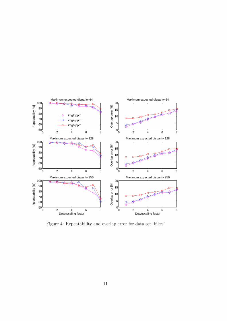
3.3.1 Blurred images—data set ‘bikes’

A set of 66 templates was matched with images of size 1000x700 pixels.For this data set we got the best repeatability results, with overall average

of 92.5%. As can be seen from Figure 4, for downscaling factors up to 6 therepeatability does not decrease below 90% for any test image.

Regarding accuracy, such results could be expected—the overlap errorrises slightly with increasing downscaling factor and image distortion.

3.3.2 Blurred images—data set ‘trees’

A set of 165 templates was matched with images of size 1000x700 pixels.Although these are another blurred images, the results differ significantly

from those of ‘bikes’. This is mainly caused by the texture-like scene type,where there are many similar indistinct features detected by Harris cornerdetector. Because of that repeatability decreases with larger search windowsas more similar regions can be found in larger areas of the same texture.

10

0 2 4 6 850

60

70

80

90

100Maximum expected disparity 64

Rep

eata

bilit

y [%

]

img2.ppm

img4.ppm

img6.ppm

0 2 4 6 80

5

10

15

20Maximum expected disparity 64

Ove

rlap

erro

r [%

]

0 2 4 6 850

60

70

80

90

100Maximum expected disparity 128

Rep

eata

bilit

y [%

]

0 2 4 6 80

5

10

15

20Maximum expected disparity 128

Ove

rlap

erro

r [%

]

0 2 4 6 850

60

70

80

90

100Maximum expected disparity 256

Rep

eata

bilit

y [%

]

Downscaling factor0 2 4 6 8

0

5

10

15

20Maximum expected disparity 256

Ove

rlap

erro

r [%

]

Downscaling factor

Figure 4: Repeatability and overlap error for data set ‘bikes’

11

This is especially true for heavily blurred test images, i.e. img4.ppm andimg6.ppm. See Figure 5 for more details.

0 2 4 6 80

50

100Maximum expected disparity 64

Rep

eata

bilit

y [%

]

img2.ppm

img4.ppm

img6.ppm

0 2 4 6 80

5

10

15

20Maximum expected disparity 64

Ove

rlap

erro

r [%

]

0 2 4 6 80

50

100Maximum expected disparity 128

Rep

eata

bilit

y [%

]

0 2 4 6 80

5

10

15

20Maximum expected disparity 128

Ove

rlap

erro

r [%

]

0 2 4 6 80

50

100Maximum expected disparity 256

Rep

eata

bilit

y [%

]

Downscaling factor0 2 4 6 8

0

5

10

15

20Maximum expected disparity 256

Ove

rlap

erro

r [%

]

Downscaling factor

Figure 5: Repeatability and overlap error for data set ‘trees’

3.3.3 JPEG compression—data set ‘ubc’

A set of 66 templates was matched with images of size 800x640 pixels.

Results for JPEG-compressed images are shown in Figure 6. As can beseen from the plots, JPEG artifacts in heavily-compressed images complicatefeature matching a lot, at least when cross-correlation is used. For example,having maximum disparity 256 and downscaling factor of 1, increasing com-pression from 60% to 90%, and then to 98%, causes the repeatability to dropfrom 100% to approximately 30%, and to 0%, respectively. For more com-pressed images repeatability can be improved by using higher downscalingfactors—for this particular data set downscaling factor 5 gives even betterresults than 2.

12

Similarly as in data set ‘trees’ the maximum expected disparity seriouslyaffects the repeatability rate. There are probably two main reasons for this:large amount of noise and many indistinctive features in test images, bothgenerated by JPEG artifacts and the rectangular grid they create.

0 2 4 6 80

50

100Maximum expected disparity 64

Rep

eata

bilit

y [%

]

img2.ppm

img4.ppm

img6.ppm

0 2 4 6 80

5

10

15

20Maximum expected disparity 64

Ove

rlap

erro

r [%

]

0 2 4 6 80

50

100Maximum expected disparity 128

Rep

eata

bilit

y [%

]

0 2 4 6 80

5

10

15

20Maximum expected disparity 128

Ove

rlap

erro

r [%

]

0 2 4 6 80

50

100Maximum expected disparity 256

Rep

eata

bilit

y [%

]

Downscaling factor0 2 4 6 8

0

5

10

15

20Maximum expected disparity 256

Ove

rlap

erro

r [%

]

Downscaling factor

Figure 6: Repeatability and overlap error for data set ‘ubc’

3.3.4 Light change—data set ‘leuven’

A set of 69 templates was matched with images of size 900x600 pixels.

Average repeatability of 84.7% was the second best result in our tests,even high downscaling factors up to 6 produce reasonable results. Repeata-bility descreases slightly with higher expected disparity. See Figure 7 formore details.

13

0 2 4 6 850

60

70

80

90

100Maximum expected disparity 64

Rep

eata

bilit

y [%

]

img2.ppm

img4.ppm

img6.ppm

0 2 4 6 80

5

10

15

20Maximum expected disparity 64

Ove

rlap

erro

r [%

]

0 2 4 6 850

60

70

80

90

100Maximum expected disparity 128

Rep

eata

bilit

y [%

]

0 2 4 6 80

5

10

15

20Maximum expected disparity 128

Ove

rlap

erro

r [%

]

0 2 4 6 850

60

70

80

90

100Maximum expected disparity 256

Rep

eata

bilit

y [%

]

Downscaling factor0 2 4 6 8

0

5

10

15

20Maximum expected disparity 256

Ove

rlap

erro

r [%

]

Downscaling factor

Figure 7: Repeatability and overlap error for data set ‘leuven’

14

3.3.5 Repeatability and accuracy discussion

Accuracy summary for each data set is provided in Table 2. When comparingresults for individual data sets it is apparent that both scene type and typeof image distortion affects accuracy and repeatability of template matching.Same type of distortion—image blur—yields different results for two differenttypes of scene. For data set ‘bikes’ we got repeatability average of 92.5%,for data set ‘trees’ we got 74.3%. Lack of distinctive features in texture-like scenes constitues a problem for other feature detectors and matchingscenarios as well. Similar results are presented in [3] where all tested detectorsperformed worse for data set ‘trees’ than for ‘bikes’.

Table 2: Repeatability and overlap error summary for data sets

Data Average Averageset repeatability overlap error

bikes 92.5% 9.4%trees 74.3% 14.9%ubc 76.5% 7.4%leuven 84.7% 8.6%

An overall conclusion can be made regarding downscaling factor. In av-erage, configurations with downscaled images had higher repeatability ratesthan those with original-sized images. From our tests the best downscal-ing factor seems to be 2 which gives an average repeatability rate 87.8%;downscaling factor 3 gives 87.5%. With templates of size 32x32 pixels, alldownscaling factors up to to 5 (86.0%) seem as a reasonable choice. Allaverages are summarized in Figure 8 and Table 3.

This might change if some filtering of original-sized images were made butthat would prevent us from taking an advantage of speed-up related to usingdownscaled images. Considering related implications to computation sizeand performance, applications should generally consider using downscaledimages for normalized cross-correlation.

For templates considered matched by the repeatability measure, overlaperror increases slightly for downscaled images, as can be seen from Figure9 and Table 4. Besides effects due to loss of information there is anotherlimitation related to the fact that integer positions are found in downscaledimages and then upscaled for the original-sized images using an integer down-scaling factor. Therefore without any sub-pixel corrections used in matching,the positions found will ideally be pixel-accurate only in 100/sd

2 per cent ofcases, with sd being the downscaling factor.

15

1 2 3 4 5 6 7 868

70

72

74

76

78

80

82

84

86

88Average repeatability

Downscaling factor

Rep

eata

bilit

y [%

]

Figure 8: Average repeatability rate vs. downscaling factor

Table 3: Average repeatability rate vs. downscaling factor

Downscaling Averagefactor repeatability

1 77.1%2 87.8%3 87.5%4 87.0%5 86.0%6 82.7%7 79.8%8 68.2%

16

1 2 3 4 5 6 7 85

6

7

8

9

10

11

12

13

14

15Average overlap error

Downscaling factor

Ove

rlap

erro

r [%

]

Figure 9: Average overlap error vs. downscaling factor

Table 4: Average overlap error vs. downscaling factor

Downscaling Average overlapfactor error

1 5.2%2 6.8%3 8.2%4 9.6%5 10.9%6 12.7%7 13.3%8 14.1%

17

3.3.6 Processing time

Effects of downscaling factor and bounded disparity field on speed shouldbe same regardless of what data set is used, provided that the number oftemplates is fixed. The results below are averages from all data sets, withthe number of templates varying from 66 to 165. Table 5 lists processingtime per template, Table 6 lists average speed-up factors for combinations ofmaximum expected disparity and downscaling factor, compared to the casewith maximum disparity 256 and no downscaling (i.e. downscaling factor 1).

Table 5: Average processing time per template [ms] for combinations ofmaximum expected disparity dmax and downscaling factor sd

dmax\sd 1 2 3 4 5 6 7 8

256 242.2 45.4 26.5 13.6 10.2 8.0 6.1 5.5128 81.0 14.5 12.1 5.5 4.5 4.0 4.0 4.164 42.1 8.1 4.8 3.9 3.5 3.5 3.4 3.1

Table 6: Average speed-up factor for combinations of maximum expecteddisparity dmax and downscaling factor sd, relatively to processing time formaximum disparity 256 and downscaling factor 1

dmax\sd 1 2 3 4 5 6 7 8

256 1.0 5.3 9.2 17.8 23.8 30.3 39.5 44.2128 3.0 16.7 20.0 44.3 53.5 60.1 60.7 58.664 5.8 30.1 51.0 61.4 68.3 69.1 71.7 78.2

As can be seen from the results, both limiting maximum expected dispar-ity and using downscaled images saves a significant amount of time. Given amaximum disparity, the computation time is reduced approximately by fac-tor of 5.4 only by increasing downscaling factor from 1 to 2. For downscalingfactor 2, which gives the highest repeatability rate, lowering maximum ex-pected disparity from 256 to 64 gives the speed-up factor of 5.6. For param-eter values considered in our tests one can get the maximum speed-up factorof 68.3 while still keeping the repeatability rate reasonably high. Note thatthe reference time itself is computed with bounded search regions, thereforespeed-up factors would be even greater if templates were matched to wholeimages.

18

3.4 Comparison to invariant features

In the last test we compare normalized cross-correlation to invariant featureswith SIFT descriptors presented in [3]. Our goal was to make the test settingsas close as possible so that the repeatability rate and matching score can becompared directly.

When comparing our results to [3], however, note that the test settingsdiffer slightly and some of the original data sets were intentionally excludedbecause of transform class.

The same test was conducted for each of the four data sets:

1. The best-performing affine detector for the data set is used to detectfeatures in the reference image. Only features present both in thereference image and in a particular test image are used. We limit themaximum number of features to 500—if more than 500 features aredetected, 500 of them are chosen randomly.

2. Templates are constructed around centers of the features; all templatesare of size 32x32 pixels.

3. These templates are then matched with test images by the templatePo-sitions function, using maximum expected disparity 425 and downscal-ing factor 4.

Maximum expected disparity of 425 was used to encompass very highdisparities in the two data sets where viewpoint changes, i.e. in data sets‘graf’ and ‘wall’.

Compared to our previous tests the number of templates is much higherand depends on the particular affine detector used. Number of invariantfeatures varies from 423 for data set ‘graf’ with the MSER detector up tothe maximum, i.e. 500.

The results, summarized in Figure 10, are very similar to those obtainedfrom the previous test for downscaling factor 4 and maximum expected dis-parity 256.3.

As assumed, invariant features out-perform normalized cross-correlationin data sets where images are related by general affine transform. This isverified on the two data sets with viewpoint changes. In data set ‘graf’normalized cross-correlation gives very poor results with repeatability notexceeding 20 per cent. In data set ‘wall’ it gives higher repeatability andmatching score than invariant features for viewpoint changes up to 30 degreesand at least comparable matching score up to 50 degrees.

3See the first plot in the third row in Figures 4, 5, 6, and 7.

19

There are probably several reasons for why these results differ so much.First, these are two types of scene—‘graf’ is structured while ‘wall’ is moretexture-like. Second, there are some additional occlusions caused by a carin images of ‘graf’. Third, viewpoint change includes rotation for some testimages of ‘graf’.

In data sets where images are related by translation-based homographies,i.e. excluding ‘graf’ and ‘wall’, normalized cross-correlation gives both higherrepeatability and matching score. This is true for all data sets except ‘ubc’where normalized cross-correlation provides comparable results up to JPEGcompression of 80 per cent. However its accuracy drops rapidly when com-pression exceeds 80 percent and then better results can be obtained withinvariant features.

Matching score of normalized cross-correlation is significantly higher forboth data sets affected by image blur: 2–3 times higher for data set ‘bikes’and 3–15 times higher for data set ‘trees’.

20 30 40 50 600

50

100

Viewpoint change

Rep

eata

bilit

y / m

atch

ing

scor

e [%

]

Data set ’graf’ − 423 templates, MSER

Cross−correlation repeatabilityMSER repeatabilityMSER with SIFT matching score

20 30 40 50 600

50

100Data set ’wall’ − 500 templates, MSER

Viewpoint change

Rep

eata

bilit

y / m

atch

ing

scor

e [%

]

2 3 4 5 60

50

100

Image blur

Rep

eata

bilit

y / m

atch

ing

scor

e [%

]

Data set ’bikes’ − 500 templates, Hessian

Cross−correlation repeatabilityHessian repeatabilityHessian with SIFT matching score

2 3 4 5 60

50

100Data set ’trees’ − 500 templates, Hessian

Image blur

Rep

eata

bilit

y / m

atch

ing

scor

e [%

]

60 70 80 90 1000

50

100

JPEG compression

Rep

eata

bilit

y / m

atch

ing

scor

e [%

]

Data set ’ubc’ − 500 templates, Hessian

Cross−correlation repeatabilityHessian repeatabilityHessian with SIFT matching score

2 3 4 5 60

50

100

Light change

Rep

eata

bilit

y / m

atch

ing

scor

e [%

]

Data set ’leuven’ − 494 templates, MSER

Cross−correlation repeatabilityMSER repeatabilityMSER with SIFT matching score

Figure 10: Comparison of normalized cross-correlation and invariantfeatures—repeatability and matching score.

20

4 Conclusions

In this paper we have described some limitations of Matlab function nor-mxcorr2 for computing normalized cross-correlation and suggested possibleimprovements for practical applications: reusing image sums when matchingmultiple templates, using bounded search regions for individual templates,and downscaling images before computation. To exploit these possibilites twoMatlab functions have been designed and implemented—normxcorr2ext andtemplatePositions. The latter has an interface convenient for object trackingand wraps the whole functionality presented in the paper.

Three tests have been carried out, using a standardized data set. First,we measured possible speed-up from reusing image sums for matching mul-tiple templates with a single image. Second, we evaluated accuracy andperformance of matching in various settings. Last, we compared normalizedcross-correlation to invariant features presented in [3].

The accuracy is measured in terms of repeatability and overlap error, asdefined in [3]. Our experiments have shown that accuracy is affected bothby type of the scene and algorithm parameters. Relatively poor results wereobtained for data sets ‘trees’ and ‘ubc’. For data set ‘trees’ it was due tolarge texture-like regions in the scene containing many indistinctive features,combined with image blur which further lowers the distinctiveness. In caseof ‘ubc’ poor results were caused mainly by JPEG compression and strongartifacts in heavily-compressed test images.

Better results in terms of repeatability were generally obtained for down-scaled images. Downscaling factor of 2 seems to be the best choice providingthe highest repeatability rates in most cases along with significant perfor-mance gain. It reduces the processing time by factor of 5, compared tothe case with original-sized images. Repeatability is reasonably high up todownscaling factor 5. As the results suggest, applications should in generalconsider to use downscaled images, although the most appropriate value ofdownscaling factor is application-dependent. The downscaling factor couldprobably be higher in applications with higher image resolution and less dis-tortion.

Using maximum expected disparity and thus bounding search regions forindividual templates also yields considerable speed-up. Lowering maximumdisparity from 256 to 64 gives an approximate speed-up factor of 5. Generalconclusion about the value of maximum expected disparity cannot be madewithout a particular application in mind—one should choose the lowest valueallowed by the application to reduce size of computation as much as possible.

Last, we compared normalized cross-correlation to invariant features withSIFT descriptors. Our results have shown that for images related by trans-

21

lation normalized cross-correlation gives both higher repeatability rate andmatching score than invariant features presented in [3].

The standardized data set provides repeatable evaluation environmentbut can be seen as too static for some object-tracking applications. Anotherevalutation in real-world scenario would probably provide deeper insight intohow to tune the parameters for real applications.

22

A User guide

A brief user guide is provided in this appendix in form of a commentedMatlab script. The output is shown in Figure 11.

%% Initialize search path for third-party functions, e.g. harris, conv2fft.

% We assume that current working directory points to the directory with

% templatePositions.m etc.

initPath

%% Load reference and test images.

% We will match templates from the reference image with the test image. We

% can load two images from the dataset ‘bikes’ used in our tests.

refImPath = ’../img/bikes/img1.ppm’;

testImPath = ’../img/bikes/img4.ppm’;

refImage = double(rgb2gray(imread(refImPath)));

testImage = double(rgb2gray(imread(testImPath)));

%% Find some feature points in the reference image.

% These will be used as template centers.

[refCenterRows refCenterCols] = featurePoints(refImPath);

%% Create templates using the feature points.

% Choosing appropriate templates for matching depends on a particular

% application...

TEMPLATE_SIZE = 32;

refCenterPos = vec2cellpos(refCenterRows, refCenterCols);

refTopleftPos = center2topleft(refCenterPos, TEMPLATE_SIZE);

[refTopleftRows refTopleftCols] = cell2vecpos(refTopleftPos);

templates = cell(1, length(refTopleftRows));

for iTpl = 1:length(refTopleftRows)

templates{iTpl} = refImage(refTopleftRows(iTpl):refTopleftRows(iTpl) ...

+ TEMPLATE_SIZE - 1, ...

refTopleftCols(iTpl):refTopleftCols(iTpl) ...

+ TEMPLATE_SIZE - 1);

end

%% Find the most likely template positions in the test image.

MIN_CORR_COEF = 0.9; MAX_DISPARITY = 64; DOWNSCALING_FACTOR = 2;

testTopleftPos = templatePositions(templates, testImage, MIN_CORR_COEF, ...

DOWNSCALING_FACTOR, refTopleftPos, MAX_DISPARITY);

testCenterPos = topleft2center(testTopleftPos, TEMPLATE_SIZE);

[testCenterRows testCenterCols] = cell2vecpos(testCenterPos);

%% Show the correspondences found.

concatImage = [refImage testImage];

demo2Fig = figure; imshow(concatImage, [0 255]); hold on;

% Plot points and matching pairs.

for iPos = 1:length(refCenterRows)

% Highlight points not matched.

if isnan(testCenterRows(iPos)) || isnan(testCenterCols(iPos))

plot(refCenterCols(iPos), refCenterRows(iPos), ’r+’, ’MarkerSize’, 10);

continue;

end

% Connect points from reference and test images.

plot([refCenterCols(iPos); testCenterCols(iPos) + size(refImage, 2)], ...

[refCenterRows(iPos); testCenterRows(iPos)], ’--g+’);

end

23

Figure 11: Matching results. Templates taken as subimages from the ref-erence image on the left were matched with the test image on the right.Correspondences are shown as dashed green lines. Templates not found us-ing the minimum correlation coefficient are highlighted red.

References

[1] Matlab documentation. normxcorr2. Available from (June 9,2010): http://www.mathworks.com/access/helpdesk/help/toolbox/images/normxcorr2.html.

[2] Lewis, J. P. Fast Normalized Cross-Correlation. Industrial Light &Magic. Available from (June 9, 2010): http://www.idiom.com/˜zilla/Work/nvisionInterface/nip.html.

[3] Mikolajczyk, K., Tuytelaars, T., Schmid, C., Zisserman, A., Matas,J., Schaffalitzky, F., Kadir, T., Van Gool, L. A Comparison ofAffine Region Detectors. International Journal of Computer Vision.Springer Science + Business Media, Inc. Available from (June 9,2010): http://www.robots.ox.ac.uk/˜vgg/research/affine/det eval files/vibes ijcv2004.pdf.

[4] Harris, C. G., Stephens, M. J. A combined corner and edge detector.Proceedings Fourth Alvey Vision Conference, Manchester. pp 147-151,1988.

[5] Svoboda, T., Kybic, J., Hlavac, V. Image Processing, Analysis, andMachine Vision: A MATLAB Companion. Thomson Learning 2008.ISBN: 0495295957.

24