Center for Biofilm Engineering

BSTM– July 2009

Al ParkerStatistician and Research EngineerMontana State University

Some statistical considerations in molecular methods

Acknowledgments

Colleagues in the CBE: James Moberly, Seth D’Imperio, Brent Peyton Markus Dieser Marty Hamilton

How to extract useful information from hundreds to thousands of response variables (eg. micro-array analysis) measured from only a few replicates (experiments or environmental samples)

The problem

Statistical thinking

Multivariate Statistics attempts to organize and summarize data sets with large numbers of response variables

“organize and summarize” = dimension reduction

In this talk, I will focus on abundance data, estimated for example from micro-array or clone analysis of PCR

Statistical thinking

Hierarchical Clustering

Principle Components

Canonical Correlation

Hierarchical Clustering (38 variables, 9 replicates)

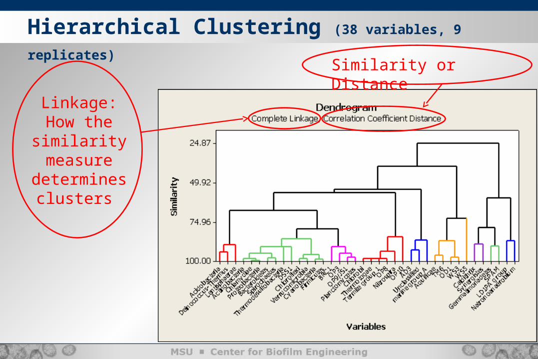
Hierarchical Clustering (38 variables, 9 replicates)

Similarity or Distance

Linkage: How the similarity measure

determines clusters

Two different ways to generate clusters

with the same similarity measure

A Distance or Similarity Measure

Correlation measures the strength and direction of a linear relationship between paired variables x and y

Corr(x,y) =(n-1)SxSy

Σ(xi – mean(x))(yi – mean(y))

Unitless Values between -1 and 1

An example (2 variables, 9 replicates)

Corr(Actinobacteria, Acidobacteria) = .7833

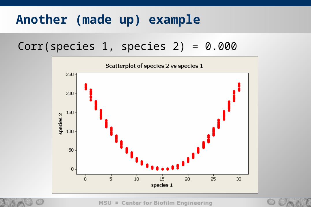
Another (made up) example

Corr(species 1, species 2) = 0.000

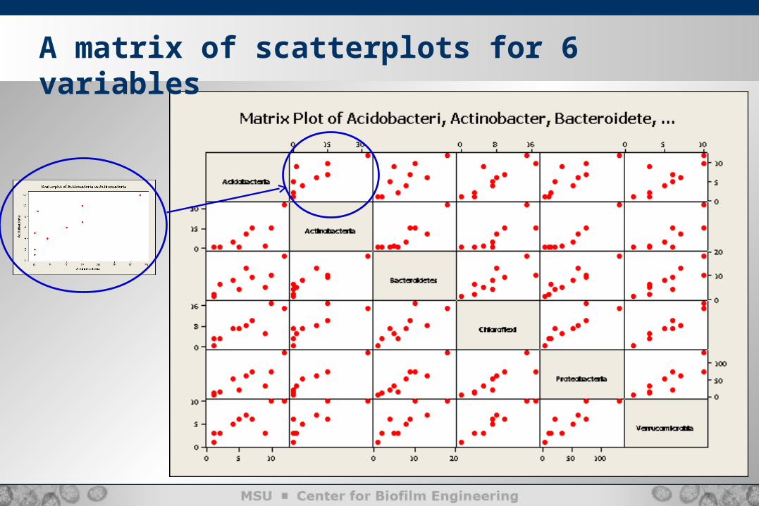
A matrix of scatterplots for 6 variables

Acidobacteria Actinobacteria Bacteroidetes Chloroflexi Proteobacteria VerrucomicrobiaAcidobacteria 1 0.7833 0.7589 0.8556 0.8444 0.7975

Actinobacteria 0.7833 1 0.8993 0.8257 0.9698 0.8230Bacteroidetes 0.7589 0.8993 1 0.7901 0.9393 0.8392Chloroflexi 0.8556 0.8257 0.7901 1 0.8704 0.9699

Proteobacteria 0.8444 0.9698 0.9393 0.8704 1 0.8621

Verrucomicrobia 0.7975 0.8230 0.8392 0.9699 0.8621 1

A correlation matrix of 6 variables

Principle Components Analysis (PCA)

PCA uses the correlation matrix formed by the original variables to optimally construct a smaller number of new variables which capture the maximum amount of variability in the original variables

PCA applied to the correlation matrix is not affected by disparate units between the different variables

The number of new variables is only as large as the number of replicates

PCA with 2 (standardized) responses

Original variable #2

Ori

gin

al vari

ab

le #

1

PCA with 2 (standardized) responses

1st PC - 78%

1st PC is loaded by Orig Var #1

Original variable #2

Ori

gin

al vari

ab

le #

1

2nd PC – 22%

2nd PC is loaded by Orig Var #2

PCA terminology

The new variables are called principle components

The amount of variability of the original data captured by each component is given

The correlation between the original variables and the principle components are principle component loadings

Reducing 7 original variables to 2 PCs

1. Water depth

2. Core depth

3. Fe

4. Mn

5. Cu

6. Pb

7. Zn

Original variables:

1st PC: Metals2nd PC: Water depth and Core depth

New variables = Principle Components

55%

18%

Reducing 7 original variables to 2 PCs

1st PC - 55%

2nd PC – 18%

Total: 73%

PCA is another way to cluster

Canonical Correlation Analysis (CCA)

CCA uses the correlation matrix to determine the (linear) relationship between input variables (eg. environmental variables) and response variables (eg. phylogenic data)

CCA simultaneously finds new variables from the input and response variables which have maximal correlation

The number of new variables (canonical components) can be no larger than the number of replicates

1. Water depth

2. Core depth

3. Fe

4. Mn

5. Cu

6. Pb

7. Zn

Original environmental variables:

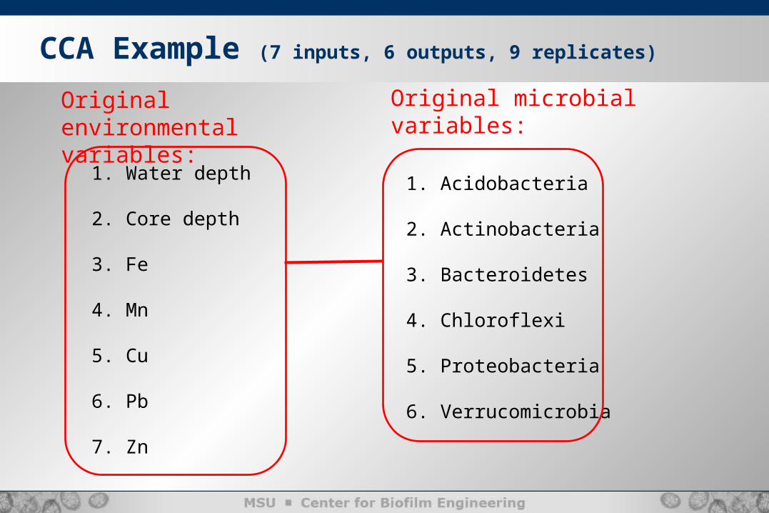
CCA Example (7 inputs, 6 outputs, 9 replicates)

1. Acidobacteria

2. Actinobacteria

3. Bacteroidetes

4. Chloroflexi

5. Proteobacteria

6. Verrucomicrobia

Original microbial variables:

1. Water depth

2. Core depth

3. Fe

4. Mn

5. Cu

6. Pb

7. Zn

Original environmental variables:

1. Acidobacteria

2. Actinobacteria

3. Bacteroidetes

4. Chloroflexi

5. Proteobacteria

6. Verrucomicrobia

Original microbial variables:

CCA (7 inputs, 6 outputs, 9 replicates)

1st CC: Water depth and Core depth

1st CC: Acidobacteria,…, Verucomicrobia

2nd CC: Metals 2nd CC: Bacteroidetes

CCA (7 inputs, 6 outputs, 9 replicates)

1st CC: Water depth and Core depth

1st CC: Acidobacteria,…, Verucomicrobia

2nd CC: Metals 2nd CC: Bacteroidetes

Summary

PROBLEM: Lots of variables measured from a few samples

SOME APPROACHES: Cluster similar variables together

Principle component analysis creates a few new variables which optimally represent the data

Canonical correlation analysis describes the optimal (linear) relationship between input and output variables

Fin

• Principal Component Analysis: water depth , core depth (, Mn-Total, Fe-Total, C

• Eigenanalysis of the Correlation Matrix

• Eigenvalue 3.8467 1.2443 1.0043 0.6628 0.1567 0.0830 0.0023• Proportion 0.550 0.178 0.143 0.095 0.022 0.012 0.000• Cumulative 0.550 0.727 0.871 0.965 0.988 1.000 1.000

• Variable PC1 PC2 PC3 PC4 PC5 PC6 PC7• water depth (cm) 0.090 -0.529 -0.732 0.338 0.131 0.201 -0.062• core depth (cm) -0.193 0.702 -0.154 0.558 0.194 0.313 0.009• Mn-Total 0.488 0.163 -0.171 -0.016 -0.366 0.084 0.752• Fe-Total 0.477 0.228 -0.126 -0.057 -0.504 0.154 -0.651• Cu-Total 0.227 -0.358 0.608 0.633 -0.119 0.188 0.004• Zn-Total 0.463 0.019 0.147 -0.326 0.634 0.505 -0.026• Pb-Total 0.474 0.142 -0.055 0.253 0.376 -0.735 -0.080

CCA (7 input variables, 9 replicates)

1st CC: Water depth Core depth

2nd CC: Metals

CCA (6 response variables, 9 replicates)

1st CC: Acidobacteria,…, Verucomicrobia

2nd CC: Bacteroidetes

Hierarchical Clustering

The large number of variables are organized into a smaller number of similar clusters

One can choose a representative variable from each cluster (eg. a mean)