CENE 486 - ceias.nau.edu
95
CENE 486 Capstone: Trax Team Wall E. Wallerson & Associates Inc. Final Report Prepared For: Bridget Bero: CENE 486 Course Grading Instructor Stephen Irwin: Project Client Prepared by: Chris Cook, Josh Endersby, and Hunter Schnoebelen CENE 486 Fall 2019 Students Tuesday 4:00pm-5:00pm December 10, 2019
Transcript of CENE 486 - ceias.nau.edu

CENE 486
Capstone: Trax Team Wall E. Wallerson & Associates Inc.
Final Report
Prepared For:
Bridget Bero: CENE 486 Course Grading Instructor
Stephen Irwin: Project Client
Prepared by:
Chris Cook, Josh Endersby, and Hunter Schnoebelen
CENE 486 Fall 2019 Students
Tuesday 4:00pm-5:00pm
December 10, 2019

1
Table of Contents 1 Project Introduction 6
1.1 Current Conditions ........................................................................................................... 8
1.2 Project Location ............................................................................................................... 9
1.3 Project Constraints/Limitations ...................................................................................... 10
2 Field Work 10
3 Testing and Analysis 12
3.1 Particle-Size Distribution ............................................................................................... 12
3.2 Hydrometer..................................................................................................................... 13
3.3 Atterberg Limits ............................................................................................................. 13
3.4 Modified Proctor Compaction ........................................................................................ 15
3.5 Triaxial Test ................................................................................................................... 15
3.6 Direct Shear .................................................................................................................... 16
3.7 Consolidation Test.......................................................................................................... 17
3.8 Heavy Metals Tests ........................................................................................................ 19
3.9 Soil Classification .......................................................................................................... 19
4 Hydrology 20
5 Hydraulics 22
6 Wall Design Alternatives 23
6.1 Concrete Cantilever Retaining Wall .............................................................................. 27
6.2 Mechanically Stabilized Earth Retaining Wall (MSE) .................................................. 33
6.3 Concrete Masonry Unit Retaining Wall ......................................................................... 36
7 Final Design Recommendation 42
8 Impacts the Design 45
8.1 Environmental Impact .................................................................................................... 45
8.2 Social Impact .................................................................................................................. 45
8.3 Economic Impact............................................................................................................ 45
9 Cost of Implementing Design 45
10 Summary of Engineering Work 46
11 Summary of Engineering Costs 51
12 Conclusion 51

2
13 References 52
Appendices 53
Appendix A- Field Safety and Sampling Plan .......................................................................... 53
Appendix B-1: Soil Test Results: Particle Size Distribution ................................................. 60
Appendix B-2: Soil Test Results: Hydrometer ...................................................................... 61
Appendix B-3: Soil Test Results: Atterberg Limits .............................................................. 63
Appendix B-4: Soil Test Results: Modified Proctor Compaction ......................................... 64
Appendix B-5: Soil Test Results: Unconfined, Unconsolidated Triaxial Compressive Test 65
Appendix B-6: Soil Test Results: Consolidation ................................................................... 65
Appendix B-7: Soil Test Results: Direct Shear ..................................................................... 66
Appendix C: Geotechnical Report ............................................................................................ 68
Appendix D: Streamstats ........................................................................................................... 77
Appendix D: Streamstats Results .............................................................................................. 78
Appendix E: Maricopa Standard Detail .................................................................................... 82
Appendix F: Reinforced CMU Wall ......................................................................................... 83
3
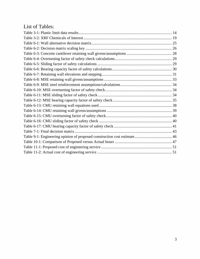
List of Tables: Table 3-1: Plastic limit data results ............................................................................................... 14
Table 3-2: XRF Chemicals of Interest .......................................................................................... 19
Table 6-1: Wall alternative decision matrix.................................................................................. 25
Table 6-2: Decision matrix scaling key ........................................................................................ 26
Table 6-3: Concrete cantilever retaining wall givens/assumptions .............................................. 28
Table 6-4: Overturning factor of safety check calculations .......................................................... 29
Table 6-5: Sliding factor of safety calculations ............................................................................ 29
Table 6-6: Bearing capacity factor of safety calculations ............................................................. 30
Table 6-7: Retaining wall elevations and stepping ....................................................................... 31
Table 6-8: MSE retaining wall givens/assumptions ..................................................................... 33
Table 6-9: MSE steel reinforcement assumptions/calculations .................................................... 34
Table 6-10: MSE overturning factor of safety check .................................................................... 34
Table 6-11: MSE sliding factor of safety check ........................................................................... 34
Table 6-12: MSE bearing capacity factor of safety check ............................................................ 35
Table 6-13: CMU retaining wall equations used .......................................................................... 38
Table 6-14: CMU retaining wall givens/assumptions .................................................................. 39
Table 6-15: CMU overturning factor of safety check ................................................................... 40
Table 6-16: CMU sliding factor of safety check .......................................................................... 40
Table 6-17: CMU bearing capacity factor of safety check ........................................................... 41
Table 7-1: Final decision matrix ................................................................................................... 43
Table 9-1: Engineering opinion of proposed construction cost estimate ...................................... 46
Table 10-1: Comparison of Proposed versus Actual hours .......................................................... 47
Table 11-1: Proposed cost of engineering service ........................................................................ 51
Table 11-2: Actual cost of engineering service ............................................................................ 51

4
List of Figures: Figure 1-1: Wall location facing east .............................................................................................. 6
Figure 1-2: Back slope location facing east .................................................................................... 7
Figure 1-3: Back slope facing west ................................................................................................. 8
Figure 1-4: Site location relative to Flagstaff ................................................................................. 9
Figure 1-5: Parcel location relative to surrounding locations ......................................................... 9
Figure 2-1: West side of sampled soil pile.................................................................................... 10
Figure 2-2: East side of sampled soil pile ..................................................................................... 11
Figure 2-3: Collected soil samples ................................................................................................ 11
Figure 3-1: Average percent finer graph ....................................................................................... 12
Figure 3-2: Fine soil particle size distribution graph .................................................................... 13
Figure 3-3: Average liquid limit graph ......................................................................................... 14
Figure 3-4: Modified proctor compaction graph .......................................................................... 15
Figure 3-5: Triaxial stress vs strain graph..................................................................................... 16
Figure 3-6: Friction angle of soil .................................................................................................. 17
Figure 3-7: Vertical stress vs strain curve..................................................................................... 18
Figure 3-8: Void ratio vs log vertical stress curve ........................................................................ 18
Figure 3-9: AASHTO soil classification....................................................................................... 20
Figure 4-1: Streamstats defined basin ........................................................................................... 21
Figure 4-2: Catch basins along route 66 ....................................................................................... 22
Figure 5-1: Weep hole Detail [9] .................................................................................................. 23
Figure 6-1: Wall alternative sketches ........................................................................................... 24
Figure 6-2: Cross-section of concrete cantilever retaining wall ................................................... 27
Figure 6-3: Concrete cantilever retaining wall profile .................................................................. 32
Figure 6-4: MSE retaining wall cross section ............................................................................... 33
Figure 6-5: MSE retaining wall profile ......................................................................................... 35
Figure 6-6: CMU retaining wall cross section .............................................................................. 36
Figure 6-7: CMU retaining wall profile ........................................................................................ 37
Figure 7-1: Flagstaff Urban Trail handrail detail .......................................................................... 44

5
Acknowledgements In the process of completing this work, the team received much help from several sources, and
would like to acknowledge the contributions of several key contributors. Thank you to our client,
Stephen Irwin, for his patience and professionalism. Thank you to Tommy Nelson, our Technical
Advisor, for his valuable knowledge and constructive input. Thank you to our grading instructor,
Bridget Bero, for her environmental engineering expertise, copious draft revisions, and taking
the time to meet with the team on a weekly basis. Thank you also to Adam Bringhurst, the lab
manager, for providing the time, equipment, and help for the lab testing. Thank you to Hanako
Ueda, the soil mechanics graduate assistant, for her help with lab testing and diagnosing testing
errors, and finally thank you to Wyatt LaFave for his help with the X-Ray Fluorescence testing.

6
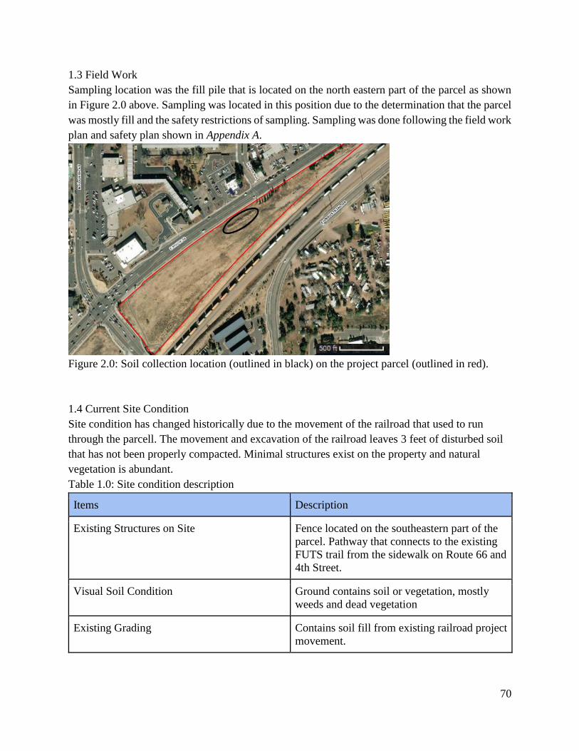
1 Project Introduction
The purpose of this project is to create a retaining wall which will allow the land owner, Holiday
Inn, to maximize the use of their land. This retaining wall will serve to stabilize the slope that
separates the grades of the Trax land and the railroad. The parcel is currently vacant and contains
excess soil fill from the 2006 relocation of the railroad tracks.
Photos of the site’s current condition were taken during site visit on 9/23. Figure 1-1 displays the
south eastern boundary of the Trax land. The proposed retaining wall will roughly parallel the
this boundary, and the picture was taken at the approximate location of the beginning of the
retaining wall. The apparent path in the picture, void of vegetation, displays what will likely be
the approximate location of the FUTS trail.
Figure 1-1: Wall location facing east

7
Figure 1-2 below, displays the slope which separates the Trax land from the Railroad. This figure
is also facing east.
Figure 1-2: Back slope location facing east

8
Figure 1-3 below, shows the North Fourth Street bridge, which represents the most southwestern
boundary of the Trax land.
Figure 1-3: Back slope facing west
1.1 Current Conditions
The current conditions on the site could be generally characterized as undeveloped and includes
a steep slope, which can be seen in Figure 1-3 above, on the northeastern property line which
separates the Trax property from the railroad. Reports from the client characterize the soil as
poor and contains fill material from the construction of the railroad.

9
1.2 Project Location
The Trax retaining wall project is located on the east side of Flagstaff, at Fourth St. and Route
66. The parcel address is 2251 E. Route 66, Flagstaff AZ 86001. Figure 1-4 below, displays the
location of the project in relation to the greater flagstaff area. the approximate project location,
the Trax land, is outlined in red. Figure 1-5 shows the property lines of the project site, and the
retaining wall will be located along the southeast property line.
Figure 1-4: Site location relative to Flagstaff
Figure 1-5: Parcel location relative to surrounding locations

10
1.3 Project Constraints/Limitations
The primary limitation to the project was the lack of proper boring equipment. This limitation
was addressed by performing the necessary soil tests on soil samples collected from the soil
stockpile on site, as opposed to split spoon samples. Another limitation on the project was the
proximity of the proposed wall to the boundary separating the Trax and Railroad properties,
which influenced the design of the wall.
2 Field Work
The field work for this project consisted of a site investigation and soil sample collection. A
safety and sampling plan was created for the field work and is appended to this report as
Appendix A. Soil sampling was conducted from 10am to noon on September 23rd, 2019. The
weather was slightly rainy and the team worked quickly to avoid being rained on. Soil conditions
were dry on top, but more moist at approximately a foot deep into the stockpile. Ambient
temperature was approximately 55 degrees Fahrenheit. Each sample was taken from a different
location along the pile. For each sample, four holes were dug into the side of the pile, two on the
north side and two in the same location but on the south side of the pile. The sample holes were
approximately one to two feet deep towards the center of the pile to avoid external weathering.
Each of the six buckets were filled from four different holes at different locations along the soil
pile. Figure 2-1 below, shows the west side of the soil sample pile where approximately half of
the soil samples were taken from.
Figure 2-1: West side of sampled soil pile

11
Figure 2-2 located below shows the east side of the soil sample pile where half of the soil
samples were taken from.
Figure 2-2: East side of sampled soil pile
Figure 2-3 located below shows the six 5-gallon buckets of soil after the soil collection process.
Figure 2-3: Collected soil samples

12
3 Testing and Analysis
Testing performed included:
1) Particle-Size Distribution
2) Hydrometer
3) Atterberg Limits
4) Sand Cone (Replaced with Modified Proctor Compaction)
5) Tri-axial
6) Consolidation
7) Direct Shear
The full results of these tests can be seen in Appendix C: Geotechnical Report. Results are
summarized in the sections below.
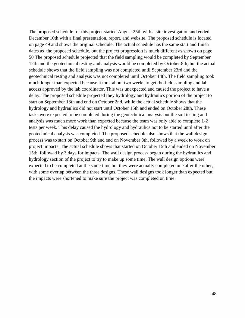
3.1 Particle-Size Distribution
The particle-size distribution test was completed in accordance with ASTM D6913.
According to this standard test procedure, the soil was sieved from the bulk composite samples
through numbers 10, 20, 40, 60, 100, 140, and 200 sieves. Each of the six samples were sieved,
and a percent finer graph was produced (Figure 3-1). Averaging the results of the six tests, it was
determined that the soil is comprised of 28.53% gravel, 65.11% sand, 5.8% silt, and 0.56% clay.
These data, along with the results of the hydrometer and Atterberg limits tests, were used to
determine the soil classification.
Figure 3-1: Average percent finer graph

13
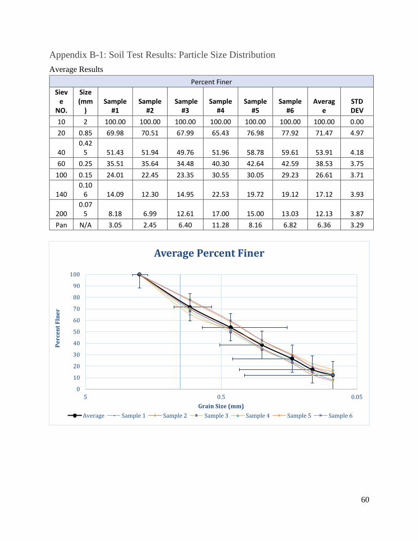
3.2 Hydrometer
The hydrometer test followed ASTM 7928-17 where only the soil that passed the number 200
sieve was tested. In order to determine the silt and clay percentages, approximately 50 grams of
each soil sample finer that the 200 sieve was placed in a 1000 milliliter graduated cylinder with
125 milliliters of sodium hexametaphosphate and 875 milliliters of water. A hydrometer was
placed in each cylinder and measurements were taken at time intervals up to 48 hours. These
measurements record how fast the soil particles settle to the bottom of the cylinder and these data
were used to determine the fine soil particle size distribution. Figure 3-2 shows each fine soil
particle size distribution as well as the average. The results show that the soil contains 65.11%
sand, 5.8% silt, and 0.56% clay. This data was used to classify the soil.
Figure 3-2: Fine soil particle size distribution graph
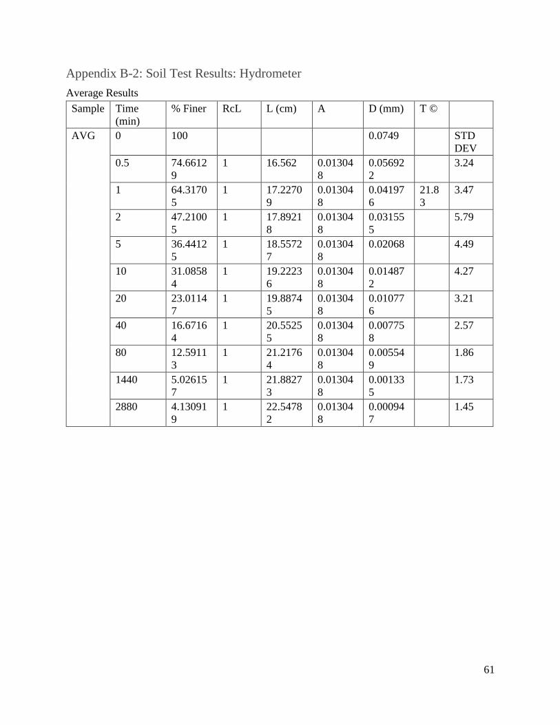
3.3 Atterberg Limits
The Atterberg Limits tests followed ASTM-D4318-17 which determined the plastic and liquid
limits. The plastic limit occurs when the moisture content of the soil reaches a level that the soil
begins to act as a plastic and the liquid limit occurs when the moisture content of the soil reaches
a level that the soil begins to act as a liquid. The plastic limit was determined by adding water to
each soil sample finer than the Number 40 sieve, and then roll it on a glass plate until the rolled
soil cracks at a diameter of 1/8th of an inch. Then the soil is dried and the moisture content and
plastic limits were determined. Table 3-1 below shows the moisture content of each sample when
the soil begins to act as a plastic, as well as the average plastic limit with the standard deviation.
14
Table 3-1: Plastic limit data results
The liquid limit also used the soil finer than the Number 40 sieve and water was added to the
soil. The soil was then placed in a Casagrande cup and a cut was made down the middle
exposing a two millimeter gap between the soil. The Casagrande cup was then raised 10
millimeters and dropped until the soil closed the gap. This was done four times for each soil
sample with different moisture contents to create a liquid limit graph. Figure 3-3 below shows
the data collected for each sample and the trend lines for each sample. Samples 4 and 5 have
dotted trend lines because the trend line slopes are positive which is incorrect so they were
excluded from the liquid limit average. The equation from the average trend line was then used
to determine the optimal moisture content at 25 drops, and that was used to determine the liquid
limit which was 24.55 percent. These limits were used to classify the soil.
Figure 3-3: Average liquid limit graph

15
3.4 Modified Proctor Compaction
The modified proctor compaction test followed ASTM-1557-12e1 to determine the dry and
moist unit weight of the soil. Soil passing the Number 4 sieve was collected from each sample
and water was added to create 4% moisture content. The soil sample was placed in the
compaction mold and the proctor hammer was dropped 25 times to compact the soil. A second
layer of soil was then placed in the mold and compacted with another 25 hammer drops. A third
layer was added and compacted, and the weight of the compacted soil was collected and then the
sample was placed in the oven to determine the moisture content. The soil had another 4%
moisture content added and the compaction process was repeated. This process of adding 4%
moisture content and then compaction was repeated until the weight of the compacted soil began
to decrease. Figure 3-4 shows the results from this test. All of the data was averaged except for
sample 4 because it does not represent the soil well. The optimal dry unit weight is 1752
(kg/m^3).
Figure 3-4: Modified proctor compaction graph
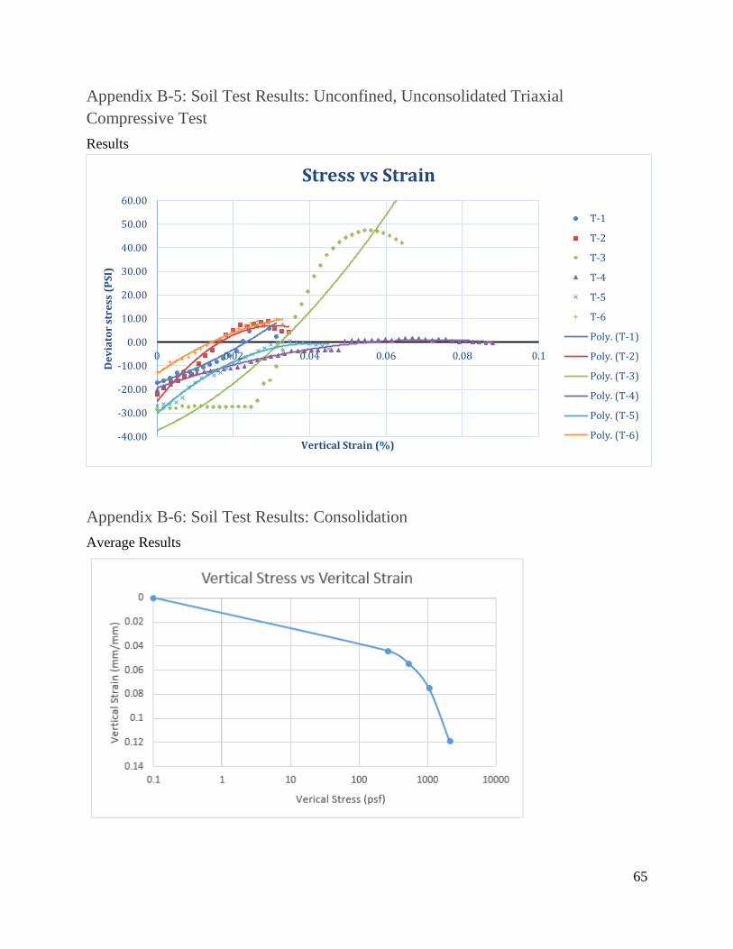
3.5 Triaxial Test
The triaxial test results are shown in Figure 3-5 below, and resulted in ambiguous data. The
specific triaxial test used was an Unconfined-Unconsolidated test, which is meant for cohesive
soils. The tested soil was composed of a large percentage of sand, which is a relatively non-
cohesive soil. This created soil specimens that could not bear much stress, and thus failed far
earlier than expected. It was determined that a direct shear test would have to be implemented to
acquire an adequate shear strength value.
16
Figure 3-5: Triaxial stress vs strain graph
The expected results from this test was to determine the soil friction angle from various
compressive strengths. The results that were obtained did not accurately represent the soil
because the majority of the soil is sand and this test is meant to test clay.
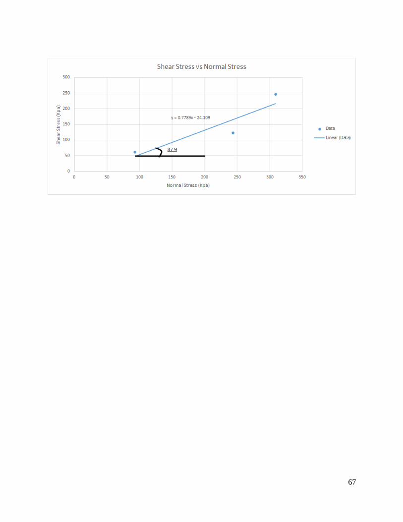
3.6 Direct Shear
The direct shear test followed ASTM D3080 to determine the friction angle of the soil. The
friction angle was initially determined by piling the dry soil and physically measuring the angle
of friction, which was determined to be 35 degrees. This friction angle was a conservative
estimate that was going to be changed after the direct shear test. The direct shear test allowed an
actual friction angle of 37.9 degrees to be determined. The actual friction angle turned out to be
larger than the bulk piled angle (35 degrees), meaning the soil is more cohesive than expected.
Figure 3-6 shows the shear stress plotted against the normal stress, which were both recorded
through a computer during the testing, and the trend line represents the angle of friction for the
soil.

17
Figure 3-6: Friction angle of soil
3.7 Consolidation Test
In order to analyze soil settlement over time, a consolidation test was run, adhering to ASTM
D2435. The objective a consolidation test is to measure settlement over time and attempt to
obtain an ultimate settlement value. In order to do this, a vertical strain versus vertical stress
curve was developed based upon the test results, and can be seen in Figure 3-7, below. The soil
was loaded to a pressure of 2099 psf, which is within the realm of what the actual bearing
conditions on sight will be under the load of the proposed retaining wall, FUTS trail, and
Holiday Inn. Under this loading, the soil reached a final settlement value of 2.47 mm or
approximately .097 inches, as displayed in the raw data of Appendix C. This low level of
consolidation is consistent with what would be expected of a soil with low levels of clay, as
identified by the soil classification methods. Lastly, Figure 3-8 displays the void ratio of the
specimen with logarithmic time. From this Figure, it can be seen that the soil contained
approximately 18% voids upon completion of compaction. This is consistent with the final
moisture content of the sample which was approximately 18%. This is displayed on the Figure as
0.1845 and since the specimen was fully saturated and under load, it can be safely assumed that
the entirety of the voids were due to the presence of water. It must be noted, that due to the time
requirements of this test (4 days to reach full loading) that only one specimen was tested.

18
Figure 3-7: Vertical stress vs strain curve
Figure 3-8: Void ratio vs log vertical stress curve

19
3.8 Heavy Metals Tests
Table 3-2 below displays the results of the heavy metal contaminants testing. The test was
performed using a Thermofisher Niton XL3T that uses X ray Fluorescence to detect
concentrations of heavy metals identified by the Arizona Soil Remediation Standard for
Residential Limits [6]. Twenty four test specimens (4 per each of the 6 samples) were placed in
the ring and cap plastic containers with a thin translucent film over the top of them. Then,
environmental consultant and NAU graduate student, Wyatt LaFave tested the samples using a
lead encased portable test stand.
Table 3-2 below, shows that the soil only slightly exceeds Arsenic and Vanadium levels. Heavy
metal contamination is not considered a concern. Table 3-2: XRF Chemicals of Interest
3.9 Soil Classification
Through the use of the AASHTO soil classification system, seen in Figure 3-9 below, the soil
has been classified as A-1-b: stone fragments, sand, and gravel. If the gravel contents were to be
20
ignored, it would change the percentage of soil passing the #40 sieve (step 5) and would then be
classified as A-3: fine sand.
Figure 3-9: AASHTO soil classification
4 Hydrology
The determination of the amount of precipitation on the parcel was completed using National
Oceanic and Atmospheric Administration, NOAA. The determination of how the water moves to
the parcel is shown as a major basin in figure 4-1. The intensity of rainfall that will be present
on site when an average storm event occurs is 0.690 inches in 10-minutes, the average amount of
precipitation for a storm in Flagstaff. All intensities that are located on the parcel are shown in
Appendix D, showing the determination of storm intensities. Using the area of the parcel, 8.7
acres, and the amount of intensity that NOAA provides, the amount of water that is present on
the parcel during a storm is 43.13 cubic ft per second on the entire parcel using the 10 year storm
data. This shows that an average 10 year storm has minimal effect on the parcel. And
precipitation that is directly on the parcel can be neglected.
The determination of the flow of water to the parcel uses stream stats to calculate the path of
flow to the parcel and the total amount of water making it to the parcel. The determination of the
amount of total water behind the wall will determine the wall restriction in design.
21
Figure 4-1: Streamstats defined basin
The movement of water on the site has been determined using the Streamstats[7] program to
delineate the major watershed that leads to the site. Streamstats determined that the amount of
flow to the parcel for the 100-year storm is 507cfs. The flow from the basin is south and floods
Fourth Street during heavy rains. Arizona Department of Transportation, ADOT, uses a series of
catch basins to move the water to an underground storm sewer. On the northern side of the
parcel, the storm drains can be seen as part of the curb and gutter on Route 66. These are
identified to be 25 feet apart and run along the full length of the parcel. This is in place due to
the flooding that happens on Fourth Street and runs into Route 66. The parcel was raised from
due to the fill during the railroad relocation in 2006, putting it slightly higher than the floodplain.
The current infrastructure that is in place will not allow flooding from the basin to reach the
parcel.

22
Figure 4-2: Catch basins along route 66
Shephard Wesnitzer Inc., SWI, has provided the drainage plans for the current site, with flow
directions and flow mitigation. The plans show that the increase in impervious surfaces (116,100
square feet because of the Holiday Inn.) The impervious surfaces will reduce the amount of
infiltration into the soil, which will allow the water on the parcel to be negligible. The drainage
plan shows that the water will be diverted from impervious surfaces to the storm sewer
management that will run underneath the FUTS trail. In conclusion, the wall will have some form
of drainage to release any excess water from behind the wall, however, this will follow a
predetermined detail. The predetermined detail will show a weep hole that will be used in the wall.
5 Hydraulics
City of Flagstaff and Coconino County do not provide standard details for retaining wall
drainage. Maricopa County design standards, also known as M.A.G.[9], were used for the
drainage of the wall. Weep holes will be spaced 20 ft apart, evenly along the base of the wall.
The holes will be made of 4” PVC pipe and cut to fit the length of the wall with a ½” slope per
foot. Maricopa County uses a filter material that is either gravel or coarse sand directly behind
the wall and filtering to the weep hole. The fill will be 18” tall and 18” wide and will run along
the base of the wall. The filter material will be determined by the contractor, and will need to be
placed between the wall and the existing soil. The final design will be using a weep holes as the
cost and will fit with the elevation change for the wall. Weep holes that will be used for the
design are shown in the design detail below.

23
Figure 5-1: Weep hole Detail [9]
6 Wall Design Alternatives
Design alternatives were determined according to the decision matrix shown in Table 6-1 below.
In the initial decision matrix, 7 possible alternatives were analyzed, using a positive, neutral, or
negative weight for the prescribed categories. Rough sketches of each of these seven wall types
can be seen in Figure 6-1, below. The seven wall alternatives included: a concrete gravity wall,
concrete cantilever wall, reinforced concrete cantilever wall, anchored retaining wall,
mechanically stabilized earth wall, concrete masonry unit wall, and a geotextile wall. Each
category was equally weighted, and the three alternatives with the highest total points were
chosen as design alternatives to be further evaluated. These more detailed designs are discussed
in Section 7.0 Final Wall Design Recommendation.

24
Figure 6-1: Wall alternative sketches

25
Figure 6-1 above, displays the 7 preliminary designs that were considered for further design. The
concrete cantilever is a conventional design option which tends to use smaller footings than its
reinforced counterpart, but trades off for depth of excavation required. Similar to the concrete
cantilever wall, a concrete gravity wall does not require reinforcement due to its sheer size and
volume, but because it tends to be a larger wall, it may not be a suitable option for this design.
An anchored retaining wall can utilize a variety of designs, but the idea is that the anchor is
attached or buried to something outside of the failure envelope of the wall. This alternative may
not be viable due to the proposed storm drain. A Mechanically Stabilized Earth retaining wall,
uses a combination of compaction and layered reinforcements to stabilize the slope. This option
may not be viable due to the proposed storm drain. A retaining wall made of Concrete Masonry
Units essentially acts as a cantilevered wall, but differs due to the lighter unit weight of the
concrete masonry units, and the thinner dimensions of the wall. Lastly, a geotextile wall utilizes
a synthetic plastic in lifts to stabilize the slope. It may also conflict with the proposed storm
drain.
Table 6-1: Wall alternative decision matrix

26
Table 6-2: Decision matrix scaling key
In the preliminary decision of which walls the team would further evaluate, the concrete gravity
wall was not considered because of its large footing and thick base, which would likely require
more land use than the project allows for. The reinforced concrete cantilever wall was not
considered because after examining the unreinforced concrete cantilever wall, it was determined
that no reinforcement was needed. The anchored wall was not considered because of the anchor
reinforcement required will add cost and time on the design as well as the drainage may be
affected by the anchor. The geotextile wall was not considered because of the complexity of the
design and the large estimated cost of the wall. The conventional cantilevered wall was chosen
because of its simplicity, the low estimated cost, and the fast estimated construction time. The
MSE wall was chosen because of its alternative material type and a more contemporary design
could be evaluated. The CMU wall was selected because of the existing CMU retaining wall that
was used on the south west side of the 4th Street bridge; this would provide a better look for the
area.
These alternatives were further evaluated through the use of a decision matrix to provide a final
design recommendation.

27
6.1 Concrete Cantilever Retaining Wall
The first wall design option is a conventional concrete cantilever retaining wall as shown in
Figure 6-2. The dimensioning for this wall were determined from the calculations that are shown
later in the report.
Figure 6-2: Cross-section of concrete cantilever retaining wall
As shown above, the designed wall is five feet high with a minimum buried depth of 2.5 feet.
The footing at the bottom of the retaining wall is 2.5 feet wide and these dimensions can be
shown in the cross-section of the wall (Figure 6-2). The values used for design, both those
determined from testing and those calculated, are located in Table 6-3. These values were used to
ensure that the concrete cantilever wall meets the minimum required factors of safety for
overturning, sliding, and bearing. These design checks are located in tables 6-4 through 6-6.

28
Table 6-3: Concrete cantilever retaining wall givens/assumptions
Givens
Heel Space Setback (ft) 1
Unit Weight γ concrete (psf) 150
Cohesion C (lb/ft^2) 0
Friction Angle Φ (degrees) 37.9
Unit Weight γ soil (psf) 109.3
7
Bearing Capacity Factor Nc 46.12
Bearing Capacity Factor Nq 33.3
Bearing Capacity Factor Nγ 48.03
Footing Depth Df (ft) 2.5
Height H (ft) 5
Footing Width B (ft) 2.5
Active Earth Pressure Coefficient Ka 0.271
5
Passive Earth Pressure Coefficient Kp 4.228
Weighted Footing Width B' (ft) 1.957
Length L (ft) 1500
Alpha α 0
Top of Wall Width Top B (ft) 1
Table 6-4 shows the calculations that were completed to determine the factor of safety check for
overturning. Overturning failure occurs when the active moment force acting on the wall is
significantly larger than the resisting moment force causing the wall to overturn. The results of
checking this design, as displayed in the green highlighted cells of Table 6-4, displays the
overturning factor of safety is 3.09, which passes the minimum of 3.0.
29
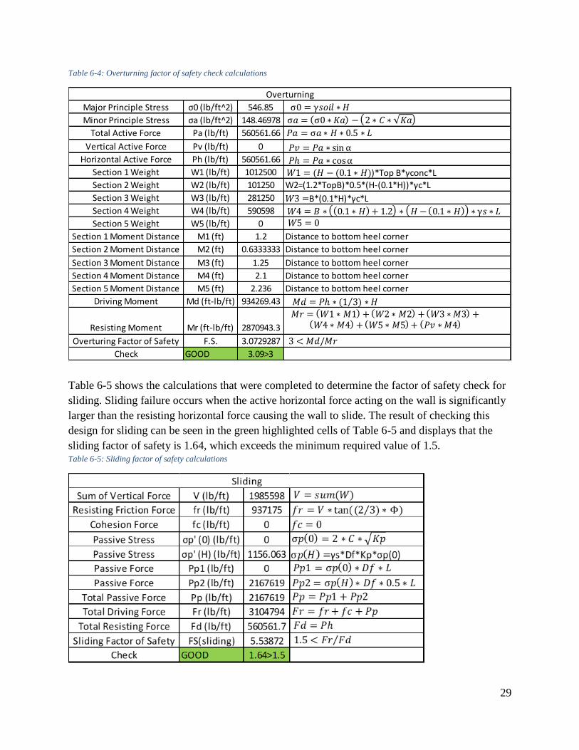
Table 6-4: Overturning factor of safety check calculations
Table 6-5 shows the calculations that were completed to determine the factor of safety check for
sliding. Sliding failure occurs when the active horizontal force acting on the wall is significantly
larger than the resisting horizontal force causing the wall to slide. The result of checking this
design for sliding can be seen in the green highlighted cells of Table 6-5 and displays that the
sliding factor of safety is 1.64, which exceeds the minimum required value of 1.5. Table 6-5: Sliding factor of safety calculations
Major Principle Stress σ0 (lb/ft^2) 546.85
Minor Principle Stress σa (lb/ft^2) 148.46978
Total Active Force Pa (lb/ft) 560561.66
Vertical Active Force Pv (lb/ft) 0
Horizontal Active Force Ph (lb/ft) 560561.66
Section 1 Weight W1 (lb/ft) 1012500
Section 2 Weight W2 (lb/ft) 101250
Section 3 Weight W3 (lb/ft) 281250
Section 4 Weight W4 (lb/ft) 590598
Section 5 Weight W5 (lb/ft) 0
Section 1 Moment Distance M1 (ft) 1.2 Distance to bottom heel corner
Section 2 Moment Distance M2 (ft) 0.6333333 Distance to bottom heel corner
Section 3 Moment Distance M3 (ft) 1.25 Distance to bottom heel corner
Section 4 Moment Distance M4 (ft) 2.1 Distance to bottom heel corner
Section 5 Moment Distance M5 (ft) 2.236 Distance to bottom heel corner
Driving Moment Md (ft-lb/ft) 934269.43
Resisting Moment Mr (ft-lb/ft) 2870943.3
Overturing Factor of Safety F.S. 3.0729287
Check GOOD 3.09>3
Overturning
)*Top B*γconc*L
W2=(1.2*TopB)*0.5*(H-(0.1*H))*γc*L
B*(0.1*H)*γc*L

30
Table 6-6 shows the calculations that were completed to determine the factor of safety check for
bearing. Bearing capacity failure occurs when the vertical bearing pressure acting on the wall is
significantly larger than the resisting pressure force pushing up on the footing causing the wall to
sink. The results of checking this design for bearing capacity can be seen in the green highlighted
cells of Table 6-6, and displays that the factor of safety for the bearing capacity was calculated as
13.08, which well exceeds the minimum required factor of safety of 3.0. Table 6-6: Bearing capacity factor of safety calculations
This wall design meets all of the retaining wall checks and works with the proximity constraints
as well as the grade elevations. Since the grade along the wall varies, the wall needed to include
steps to keep the minimum depth at 2.5 feet and to keep the top of wall one-foot minimum above
grade. Table 6-7 includes the grade elevations along the wall as well as the elevations of the top
and bottom of the wall. It also includes the step locations and the above and below grade values.
Table 6-7 shows the stationing of the wall starting from the west side, and provides the grade
elevation, top and bottom of wall elevations, stepping locations, step sizes, and the above and
below grade lengths of the wall.
Pressure q (lb/ft) 410137.5
Shape Factor Fqs 1.001012 From Table
Shape Factor Fγs 0.99948 From Table
Depth Factor Fqd 1.231638 From Table
Depth Factor Fγd 1 From Table
Momnent Difference Mn (ft-lb/ft) 1936674
Eccentricity e (ft) 0.274639
Maximum Pressure q_max (lb/ft^2) 1317750
Minimum Pressure q_min (lb/ft^2) 270728.5
Beta β (degrees) 0
Inclination Factor Fqi 1 From Table
Inclination Factor Fγi 1 From Table
Bearing Capacity qu (lb/ft^2) 16843340
Bearing Factor of Safety F.S. 12.78189
Check GOOD 13.08>3
Bearing Capacity

31
Table 6-7: Retaining wall elevations and stepping

32
Figure 6-3 below, shows a plan view of the concrete cantilever design discussed above. This
alignment utilized very few steps, since the wall remains the same height throughout the
alignment.
Figure 6-3: Concrete cantilever retaining wall profile

33
6.2 Mechanically Stabilized Earth Retaining Wall (MSE)
The second design alternative is a Mechanically Stabilized Earth retaining wall shown in Figure
6-4. The dimensioning for this design was determined from the calculations that are shown later
in the report.
Figure 6-4: MSE retaining wall cross section
Table 6-8 shows the given values from the soil testing as well as the assumed height of the wall.
The assumed wall height was determined by inputting various heights into the calculations until
the factor of safety checks met the requirements. Table 6-8: MSE retaining wall givens/assumptions
Givens
Friction Angle Φ 37.9 Given
Soil Unit Weight γ (psf) 109.37 Given
Cohesion C 0 Given
Height H (ft) 5 Assume
Table 6-9 shows the assumed steel strip dimensions and calculations used to determine the length
of the steel straps. The purpose of this table was to determine the required length of the steel
straps. The dimensions and spacing of the straps were assumed through a trial and error process
to determine the required length of the steel straps, which is 10 feet.

34
Table 6-9: MSE steel reinforcement assumptions/calculations
Table 6-10 shows the calculations used to determine the overturning factor of safety. The result
from this table is highlighted in green which shows that the overturning factor of safety is greater
than the required value of 3. Table 6-10: MSE overturning factor of safety check
Table 6-11 shows the calculation used to determine the sliding factor of safety. The result from
this table is highlighted in green which shows that the sliding factor of safety is greater than the
required value of 3. Table 6-11: MSE sliding factor of safety check
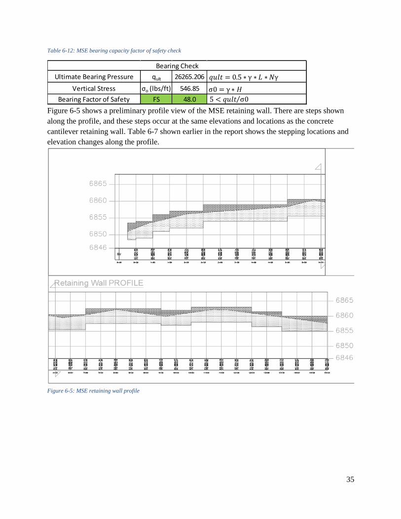
Table 6-12 shows the calculations used to determine the bearing capacity factor of safety. The
result from this table is highlighted in green which shows that the bearing capacity factor of
safety is greater than the required value of 3.
Width of Tie w (in) 2.00 Assume
Vertical Tie Spacing SV (ft) 1.25 Assume
Horizontal Tie Spacing SH (ft) 4.00 Assume
Yield Strenght of Tie fy (lbs/ft^2) 5012504.23 Assume
Soil-Tie Friction Angle Φu 20 Assume
Tie Thickness t (in) 0.057594397
Corrosion Tie Thickness tc (in) 0.12
Breaking Factor of Safety FSB 3 Assume
Pulling Factor of Saftey FSP 3 Assume
Lateral Pressure σa (lbs/ft) 267.31
Active Pressure Coefficient Ka 0.489
Steel Strap Length L 10
Steel Reinforcement
Soil Weight W 5468.5
Distance to Soil Load x 5
Lateral Soil Force Pa 668.3
Depth of Lateral Force z 1.67
Overturining Factor of Safety FS 24.5
Overturing Check
Sliding Factor of Safety FS 3.86
Sliding Check
35
Table 6-12: MSE bearing capacity factor of safety check
Figure 6-5 shows a preliminary profile view of the MSE retaining wall. There are steps shown
along the profile, and these steps occur at the same elevations and locations as the concrete
cantilever retaining wall. Table 6-7 shown earlier in the report shows the stepping locations and
elevation changes along the profile.
Figure 6-5: MSE retaining wall profile
Ultimate Bearing Pressure qult 26265.206
Vertical Stress σo (lbs/ft) 546.85
Bearing Factor of Safety FS 48.0
Bearing Check

36
6.3 Concrete Masonry Unit Retaining Wall
The third design alternative will be a Concrete Masonry Unit retaining wall which has a cross-
section shown in Figure 6-6. Figure 6-6 includes the dimensions of the wall as well as the
varying wall heights/base widths that occur along throughout the length of the wall. The wall
heights vary because the depth of footing was maintained at 5 feet while the top of wall varied as
the elevation of the finished grade changed along the alignment. The table in the upper right
corner of Figure 6-6 shows the different heights used along the wall with the footing sizes for
that wall height. The rebar required in the footing and stem was designed from the ACI
Reinforced Concrete Code [11].
Figure 6-6: CMU retaining wall cross section
Figure 6-7 includes the profile of the wall, which shows that the wall includes steps at various
locations along the top and bottom of the wall. The footing along the profile never exceeds the
30 inch frost depth and the top of the wall steps half a foot or less whenever the finish grade
elevation is equal to the top of the wall elevation.
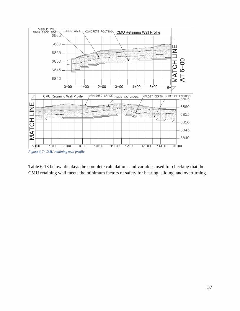
37
Figure 6-7: CMU retaining wall profile
Table 6-13 below, displays the complete calculations and variables used for checking that the
CMU retaining wall meets the minimum factors of safety for bearing, sliding, and overturning.

38
Table 6-13: CMU retaining wall equations used
Table 6-14 below, displays some of the more important values used in the design checks.

39
Table 6-14: CMU retaining wall givens/assumptions

40
Table 6-15 below, displays the design check to ensure that factor of safety for overturning for the
tallest section of the CMU retaining wall meets the required minimum. From the cells
highlighted in green, it can be seen that the design meets the minimum required factor of safety
of 3.0.
Table 6-15: CMU overturning factor of safety check
Table 6-16 below, displays the design check to ensure that factor of safety for sliding for the
tallest part of the CMU retaining wall meets the required minimum. From the cells highlighted in
green, it can be seen that the design meets the required minimum factor of safety for sliding of
1.5. Table 6-16: CMU sliding factor of safety check
Table 6-17 below, displays the design check to ensure that the tallest section of the CMU
retaining wall meets the minimum required factor of safety for bearing capacity. From the cells
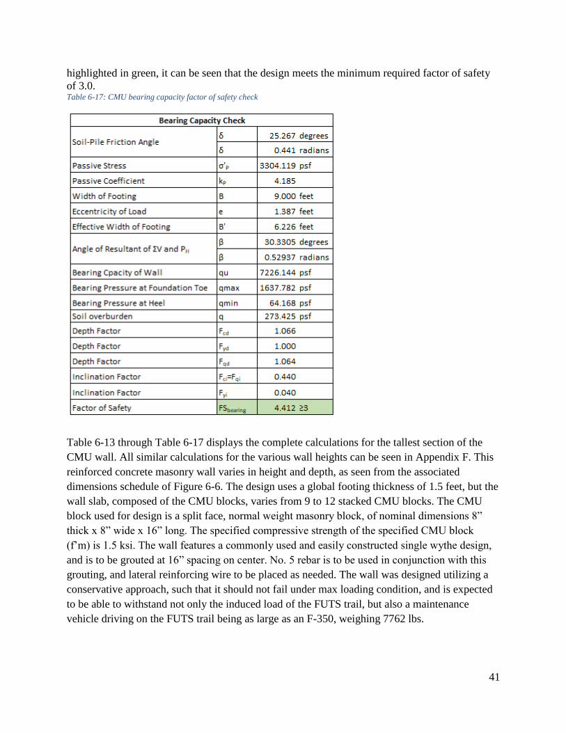
41
highlighted in green, it can be seen that the design meets the minimum required factor of safety
of 3.0. Table 6-17: CMU bearing capacity factor of safety check
Table 6-13 through Table 6-17 displays the complete calculations for the tallest section of the
CMU wall. All similar calculations for the various wall heights can be seen in Appendix F. This
reinforced concrete masonry wall varies in height and depth, as seen from the associated
dimensions schedule of Figure 6-6. The design uses a global footing thickness of 1.5 feet, but the
wall slab, composed of the CMU blocks, varies from 9 to 12 stacked CMU blocks. The CMU
block used for design is a split face, normal weight masonry block, of nominal dimensions 8”
thick x 8” wide x 16” long. The specified compressive strength of the specified CMU block
(f’m) is 1.5 ksi. The wall features a commonly used and easily constructed single wythe design,
and is to be grouted at 16” spacing on center. No. 5 rebar is to be used in conjunction with this
grouting, and lateral reinforcing wire to be placed as needed. The wall was designed utilizing a
conservative approach, such that it should not fail under max loading condition, and is expected
to be able to withstand not only the induced load of the FUTS trail, but also a maintenance
vehicle driving on the FUTS trail being as large as an F-350, weighing 7762 lbs.

42
7 Final Design Recommendation
In order to determine the final wall design recommendation, a second decision matrix was
performed, which comparatively evaluated the three alternatives that were chosen to be further
developed after the preliminary decision matrix. This decision matrix featured a more in depth
explanation of the 6 grading criteria and can be seen below in Figure 7-1 below. These grading
criteria were composed of 6 major criteria to determine the most feasible option for the client.
These criteria were:
1) The ability to easily implement drainage, such as weep holes, into the design.
2) The size of foundation as the railroad restricts the size of the foundation at the toe to 6
inches.
3) The amount of reinforcement required, evaluated from both economic and construction
standpoints.
4) The aesthetics of the wall, based upon its cohesive appearance with the surrounding
infrastructure.
5) Cost of construction and implementation.
6) The estimated time of construction.

43
Table 7-1: Final decision matrix
As can be seen in Table 7-1, the final wall recommendation is the CMU wall design. This design
features a normal weight CMU split face brick with nominal dimensions 8” x 8” x 16” with a
compressive masonry strength (f’m) equal to 1.5 ksi. The smallest section of the wall utilizes 9
blocks stacked, and stepping occurs by 1 block up to a maximum of 12 blocks. Type M mortar is
to be used along the lateral joints of the CMU blocks, and every other block column is to be
grouted. The grouted cells are to have one #7 rebar placed in the center of the cell. In the footing,
three #7s per foot are to be placed four inches below the top of the footing. The wall was
designed using a conservative approach, meaning that the wall should not fail under maximum
loading conditions, which includes the surcharge of a maintenance vehicle weighing as much as
7762 lbs.

44
The client asked for a railing that would match the standards for the City of Flagstaff, which is
shown in Figure 7-1. Using the engineering detail 14-01-010 from the city, the contractor will
attach the railing to the top of the CMU retaining wall [10]. It will be up to the contractor how
the railing will be mounted to the wall, however, the contractor is required to follow the details
in the construction plan set.
Figure 7-1: Flagstaff Urban Trail handrail detail

45
8 Impacts the Design
8.1 Environmental Impact
The environmental impact this project may have would be the large amount of concrete that is
required for the footing. The footing for the wall requires concrete that will most likely have to
be transported from Phoenix, Arizona. The transportation of the concrete and the pouring will
produce CO2 that pollutes the air. The construction of the wall will cause noise pollution for
nearby businesses.
8.2 Social Impact
The social impact this project would have is the extension of the FUTS path with the retaining
wall being located next to the path. The retaining wall with the handrail will support the path
extension and provide better access through the area for pedestrians and bike. The handrail will
also help prevent people from walking or falling into the railroad. This retaining wall will also
have the same look as the existing retaining walls on the west side of the 4th Street bridge so the
proposed wall will continue the aesthetic look of the surrounding location.
8.3 Economic Impact
The primary economic impact of this project is to support local businesses, from buying
construction materials from local manufacturers in Flagstaff. The CMU blocks that are proposed
in the retaining wall design can be manufactured and purchased in Flagstaff. Masonry contractor
are also common in Flagstaff so this project would also support their business. Also, the handrail
used in the proposed design is a Flagstaff standard handrail with is used all around the city so the
manufacturing and installation of that handrail will also be done locally.
9 Cost of Implementing Design
The total costs of implementation for the CMU design alternative is displayed below in Table 9-
1. These costs were developed using the 2005 version of the RS Means Cost of Construction
book [8]. The costs estimates form RS Means Cost of Construction include the labor and
material costs. Maintenance may also be required which could include spraying the wall with salt
to reduce the freeze thaw process that occurs in Flagstaff as well as cleaning weep holes and
checking for cracks. The majority of the maintenance that will be required for this project will be
on the FUTS trail because the trail will have users. The maintenance for this project will be
conducted by the City of Flagstaff.

46
Table 9-1: Engineering opinion of proposed construction cost estimate
10 Summary of Engineering Work
Summaries of the proposed engineering design hours and the actual engineering design hours
completed are shown in Figures 10-1. Comparing the two tables, one can see a number of
discrepancies between what was proposed and what actually occurred. First it was originally
proposed that the field work would take approximately 30 hours, but as discussed in the Field
Work Plan, the soil sample acquisition methods incurred some unexpected difficulties that
ultimately simplified sample collection greatly, so that the actual sample collection took only 5.5
hours total. Second, the scope of the soil testing expanded beyond that which was originally
proposed, but took only 2 hours longer than what was originally expected. Third, as discussed in
Section 11.0, the existing surface water runoff conveyance of the area surrounding the site and
the proposed storm drain on site greatly simplified the work on hydrology and hydraulics, cutting
84 hours of proposed work to 18 hours of actual work for those tasks. Last, the inherently
ambiguous nature of project management led to a total discrepancy of approximately 70 hours
(about 25%), compared to the proposed, across the sum of all the subtasks associated with that
major task.

47
Table 10-1: Comparison of Proposed versus Actual hours
48
The proposed schedule for this project started August 25th with a site investigation and ended
December 10th with a final presentation, report, and website. The proposed schedule is located
on page 49 and shows the original schedule. The actual schedule has the same start and finish
dates as the proposed schedule, but the project progression is much different as shown on page
50 The proposed schedule projected that the field sampling would be completed by September
12th and the geotechnical testing and analysis would be completed by October 8th, but the actual
schedule shows that the field sampling was not completed until September 23rd and the
geotechnical testing and analysis was not completed until October 14th. The field sampling took
much longer than expected because it took about two weeks to get the field sampling and lab
access approved by the lab coordinator. This was unexpected and caused the project to have a
delay. The proposed schedule projected they hydrology and hydraulics portion of the project to
start on September 13th and end on October 2nd, while the actual schedule shows that the
hydrology and hydraulics did not start until October 15th and ended on October 28th. These
tasks were expected to be completed during the geotechnical analysis but the soil testing and
analysis was much more work than expected because the team was only able to complete 1-2
tests per week. This delay caused the hydrology and hydraulics not to be started until after the
geotechnical analysis was completed. The proposed schedule also shows that the wall design
process was to start on October 9th and end on November 8th, followed by a week to work on
project impacts. The actual schedule shows that started on October 15th and ended on November
15th, followed by 3 days for impacts. The wall design process began during the hydraulics and
hydrology section of the project to try to make up some time. The wall design options were
expected to be completed at the same time but they were actually completed one after the other,
with some overlap between the three designs. These wall designs took longer than expected but
the impacts were shortened to make sure the project was completed on time.

49

50

51
11 Summary of Engineering Costs
The proposed summary of engineering costs, can be seen in Figure 11-1 below. The summary of
the actual costs can be seen in Figure 11-2, below Figure 11-1. Comparing the two, it can be seen
that the design fee was approximately ⅔ of the proposed design fee. The greatest contributors to
this discrepancy were the discrepancies between proposed and actual hours on the project due to
soil testing and the simplified hydrological analysis. It can be seen in Figure 11-1 that the actual
cost of engineering services incurred by the client was $60,815. Table 11-1: Proposed cost of engineering service
Table 11-2: Actual cost of engineering service
12 Conclusion
The objective of this project was to produce three possible retaining wall design alternatives
which would adequately support the proposed FUTS trail and Holiday Inn. Prior to designing the
alternatives, soil analysis was needed to determine the type of soil that was retained. The soil
testing along with the determination of other soil property factors, were used to evaluate the wall
designs. The three alternatives were determined based on decision matrices to narrow the best
option. This final recommendation was determined to be a CMU wall that was adjusted based on
the existing grade and the client’s proposed grade. The project was completed on time.

52
13 References
[1] Gismaps.coconino.az.gov. (2019). Coconino Parcel Viewer. [online] Available at:
https://gismaps.coconino.az.gov/parcelviewer/ [Accessed 25 Feb. 2019].
[2] Earth.google.com. (2019). Google Earth. [online] Available at: https://earth.google.com/web/
[Accessed 25 Feb. 2019].
[3] Compass.astm.org. (2019). ASTM International - Compass Login. [online] Available at:
https://compass.astm.org/EDIT/html_annot.cgi?D4767+11 [Accessed 28 Feb. 2019].
[4] N. Braja M. Das, Principles of Foundation Engineering, 9 ed., Boston, Massachusetts: Cenage,
2017.
[5] M.-C. R. Y. W. A. K. Donald P Coduto, Geotechnical Engineering, Second Edition ed.,
Pearson Education, 2011.
[6] Arizona Department of Environmental Quality, "Department of Environrmental Quality -
Remedial Action," 31 March 2009. [Online]. Available:
https://apps.azsos.gov/public_services/Title_18/18-07.pdf.
[7] "StreamStats", Streamstats.usgs.gov, 2019. [Online]. Available:
https://streamstats.usgs.gov/ss/. [Accessed: 16- Oct- 2019].
[8] RS Means 2005, Estimating in Building Constriction, S. Peterson, F. Dagostino
[9]“Programs,” AZMAG. [Online]. Available: https://www.azmag.gov/Programs/Public-
Works/Specifications-and-Details. [Accessed: Dec-2019].
[10]Flagstaff.az.gov. (2019). Engineering Design Standards | City of Flagstaff Official Website.
[online] Available at: https://www.flagstaff.az.gov/482/Engineering-Design-Standards [ Dec.
2019].
[11]Concrete.org. (2019). 318 Building Code Portal. [online] Available at:
https://www.concrete.org/tools/318buildingcodeportal.aspx.aspx

53
Appendices
Appendix A- Field Safety and Sampling Plan
Trax Retaining Wall Team Field Work Plan
Wall E. Wallerson Inc. and Associates
Josh Endersby
Hunter Scnoebelen
Chris Cook
9/18/2019
Figure 1: Project Location in Flagstaff, Arizona

54
1.0 Sampling Location:
Figure 2.0: Sampling Location
2.0 Sampling The Trax Team plans to acquire a total of 4-8 samples from 4 soil piles. The soil piles,
shown in Figure 2.0: Sampling Locations, show that the sampling will start from the undeveloped
lot West of Fourth Street while the rest of the sampling will occur on the East side of the site.
Samples will be taken at multiple locations around the soil piles and placed in a five-gallon bucket.
Each pile samples will be placed in different buckets and labeled accordingly.
2.1 Equip The equipment that will be used for sample collection will include:
● 3 shovels
● 3 pairs of working gloves
● maximum of 8 five-gallon buckets
● Hand auger (if necessary)
● tape and sharpie for labeling samples.
2.2 Sample Protocol Per each soil pile, the soil on the outside will be scraped off of the pile to eliminate
weathered soil from the sample. The samples will then be in areas around the pile, as shown in
Figure 3.0. The samples will be taken as close to the center of the pile as possible to provide an
accurate representation of the entire pile. The soil sampled from each location around the pile will
be placed in a bucket and label to prevent confusion. The labels will include a “T” for Trax, and a
number representing which pile the soil was taken from. An example would be “T-1” for pile 1, if
multiple sample buckets are used on the same pile the labeling would be “T-1.1” and “T-1.2”.

55
Figure 3.0: Sapling Method
2.3 Deviations from Plan
In the event that the team is unable to acquire the samples in the manner(s) described above, the
following deviations will be executed as necessary.
1. If dense, large rock is uncovered, preventing the acquisition of a sample, then smaller
samples will be taken at any possible location around the pile.
2. If an acceptable sample cannot be obtained for lab testing, the pocket penetrometer and
Torvane tests will be used in place of the triaxial test.
3. After speaking to the client, the team is aware that there is a large amount of fill and “bad
soil” on the site. If the tests or samples indicate something other than these results, the
client will provide the team with the geotechnical report to use for design
4. In the very worst-case event, that no good sample can be acquired, the team will discuss
with the Technical Advisor and Client the option to entirely replace the geotechnical
testing with a site survey.
3.0 Safety In the event of an emergency, the nearest hospital is the Flagstaff Medical Center,
located at 1200 N Beaver St, Flagstaff, AZ, 86001. This location is approximately 3 miles or 8
minutes away from the site. The map below shows the approximate times and distances of
alternate routes to the hospital.

56
Figure 3.0: Emergency Route Map
The map shows that the two main routes are either:
West along Route 66 to Switzer Canyon Drive,
North to San Francisco Street,
Hospital on left
Or
Go North on Fourth Street,
(Sub-option: Take E 6th Ave to N West St)
To West on E Cedar Ave
E Cedar turns into E Forest Ave
Follow E Forest Ave West to San Francisco Street
South on San Francisco St,
Hospital on Right.

57
NAU Field Safety Checklist
This form is designed to assist the Principal Investigator (PI), or Supervisor with assessing potential hazards of
fieldwork. The completed checklist must be shared with all the members of the field team and a copy must
be kept on file on campus. Multiple trips to the same location can be covered by a single checklist, as long as any
changes in hazards and/or participants are documented. NAU’s Regulatory Compliance groups are available to
review these plans, and will conduct periodic reviews of departmental checklists.
Before you go: ¨This checklist must be completed, with a copy maintained on campus, prior to departure for any fieldwork. ¨Prepare first aid kit and any documentation needed (SOPs, Chemical Safety Data Sheets, etc) ¨Assemble and check safety provisions ¨Check to assure all required immunizations are current for all team members ¨Check to assure all emergency health care and insurance requirements have been met.
Principal Investigator/Supervisor: Bridget Bero
Type of Field Work: Academic Field Trip Field Research Observation Other
Dates of Travel: September 23, 2019
Mode of Transportation: Personal Vehicle
Location of Field Work: Country: USA Geographical Site: 4th Street/Route 66
Nearest City: Flagstaff, AZ Distance from
Site: 0 Miles Nearest Hospital/Distance (Attach map when applicable):
See attached
Field Work: The team plans to sample soil from existing piles with shovels and buckets. The samples will
then be transported back to the soils lab in the engineering building.
No-Go Criteria: High winds, thunderstorms (lightning within 6 miles or 30 seconds for thunder to sound)

58
Emergency Procedures: See attached
University Contact (Name/ Phone): Adam Bringhurst/435-668-6799
Local Field Contact (Name/ Phone): Stephen Irwin/928-242-5641
Special Medical Requirements: None
First Aid Training: None
Physical Demands: Carrying and lifting 5-gallon buckets filled with soil. Shoveling the soil from test piles.
Risk Assessment: Please list identified risks associated with the activity or the physical
environment and the appropriate safety measures to be taken to reduce the risks (personal
protective equipment, training, SOPs, etc); Include a separate sheet if necessary. Attach
Safety Data Sheets (SDSs) and training documentation for any chemicals that will be used.
Identified Risk Safety Measures
Temperature Extremes Team will not go out in the field if temperatures are below 30
or above 90 degrees.
Cuts From Vegetation
Wear closed toe shoes and pants
Plants/Insect Allergies
Route to hospital planned, and first aid kit in nearby car
Tripping
Work in the daytime and stay back from the road property
Blisters
Wear work gloves

59
Animal Studies: A field study is defined as any study conducted on free-living wild animals
that does not involve an invasive procedure or materially alter the behavior of the animal under
study. In order to help you determine if your study fits this criteria, please answer the following
questions.
1. Does your study greatly disturb the animals under study?YesNo
(ex. testing predator vocalization, supplemental feeding, nest manipulation)
2. Does your study involve an invasive procedure? YesNo
(ex. blood sampling, tagging)
3. Does your study cause potential harm/injury to the animal? YesNo
(ex. net and trap capture, bagging)
If you answered YES to any of these questions, your study involves invasive procedures or
materially alters the behavior of the animal under study. Please fill out the full IACUC
protocol application form. http://www.research.nau.edu/compliance/iacuc/
If you answered NO to all three of these questions and your study will only involve
observation of free ranging animals, then an IACUC protocol is not required.
Field Team Membership (Please list the names of all members of the field team, and the
Field Team Leader.) Include a separate sheet if necessary.
Name/Cell Phone Number (if applicable on site)
1. Chris Cook, 951-970-0947
2. Josh Endersby, 760-468-9711
3. Hunter Schnoebelen, 623-680-8462
60
Appendix B-1: Soil Test Results: Particle Size Distribution
Average Results
Percent Finer
Sieve
NO.
Size (mm
) Sample
#1 Sample
#2 Sample
#3 Sample
#4 Sample
#5 Sample
#6 Averag
e STD DEV
10 2 100.00 100.00 100.00 100.00 100.00 100.00 100.00 0.00
20 0.85 69.98 70.51 67.99 65.43 76.98 77.92 71.47 4.97
40 0.42
5 51.43 51.94 49.76 51.96 58.78 59.61 53.91 4.18
60 0.25 35.51 35.64 34.48 40.30 42.64 42.59 38.53 3.75
100 0.15 24.01 22.45 23.35 30.55 30.05 29.23 26.61 3.71
140 0.10
6 14.09 12.30 14.95 22.53 19.72 19.12 17.12 3.93
200 0.07
5 8.18 6.99 12.61 17.00 15.00 13.03 12.13 3.87
Pan N/A 3.05 2.45 6.40 11.28 8.16 6.82 6.36 3.29
0
10
20
30
40
50
60
70
80
90
100
0.050.55
Pe
rce
nt
FIn
er
Grain Size (mm)
Average Percent Finer
Average Sample 1 Sample 2 Sample 3 Sample 4 Sample 5 Sample 6
61
Appendix B-2: Soil Test Results: Hydrometer
Average Results
Sample Time
(min)
% Finer RcL L (cm) A D (mm) T ©
AVG 0 100 0.0749 STD
DEV
0.5 74.6612
9
1 16.562 0.01304
8
0.05692
2
3.24
1 64.3170
5
1 17.2270
9
0.01304
8
0.04197
6
21.8
3
3.47
2 47.2100
5
1 17.8921
8
0.01304
8
0.03155
5
5.79
5 36.4412
5
1 18.5572
7
0.01304
8
0.02068 4.49
10 31.0858
4
1 19.2223
6
0.01304
8
0.01487
2
4.27
20 23.0114
7
1 19.8874
5
0.01304
8
0.01077
6
3.21
40 16.6716
4
1 20.5525
5
0.01304
8
0.00775
8
2.57
80 12.5911
3
1 21.2176
4
0.01304
8
0.00554
9
1.86
1440 5.02615
7
1 21.8827
3
0.01304
8
0.00133
5
1.73
2880 4.13091
9
1 22.5478
2
0.01304
8
0.00094
7
1.45

62
0
10
20
30
40
50
60
70
80
90
100
00.010.020.030.040.050.060.070.08
Per
cen
t F
iner
Particle Diamter Size (mm)
T-1
T-2
T-3
T-4
T-5
T-6
AVERAGE
Clay
Silt
Sand
63
Appendix B-3: Soil Test Results: Atterberg Limits
Average Results
Plastic Limit
Moisture Can ID T-1 T-2 T-3 T-4 T-5 T-6
Mc (g) 19.5 13.3 19.8 13.6 13.2 13.3
Mm (g) 31.6 25.2 27.5 24.2 31 22.4
Md (g) 29.2 23.2 26 22.2 27.7 20.7
w (%) 24.74 20.20 24.19 23.26 22.76 22.97
PL (%) 24.74 20.20 24.19 23.26 22.76 22.97
AVG PL (%) 23.02 ± 1.58
LL 24.552
y = -0.1128x + 27.372
20
21
22
23
24
25
26
27
28
29
10 15 20 25 30 35 40 45 50
Mo
uis
ture
Co
nte
nt
(%)
Number of Drops
Liquid Limit (LL)
T-1
T-2
T-3
T-4
T-5
T-6
Average
LL
LL
Linear (T-1)
Linear (T-2)
Linear (T-3)
Linear (T-4)
Linear (T-5)
Linear (T-6)

64
Appendix B-4: Soil Test Results: Modified Proctor Compaction
Average Results
Modified Proctor Compaction- Average
Trial 1 2 3 4 5
moisture content 0.040 0.082 0.116 0.163 0.201
Std Dev Moisture Content 0.003 0.012 0.005 0.006 0.009
weight of compacted soil 1571.
9 1675.
7 1803.
6 1919.
3 1845.
2
moist unit weight 1667.
6 1777.
8 1913.
6 2036.
2 1955.
3
dry unit weight 1588.
1 1619.
7 1684.
6 1751.
2 1628.
6
Std Dev Dry Unit Weight 23.3 17.8 14.8 21.1 11.0
Optimal dry unit weight 1752
Optimal dry unit weight (lb/ft^3) 109.3
7
1550.0
1600.0
1650.0
1700.0
1750.0
1800.0
1850.0
0.000 0.050 0.100 0.150 0.200
Dry
Un
it W
eigh
t (k
N/m
^3
)
Moisture Content (g/g)
Modified Proctor Compaction
T-1
T-2
T-3
T-4
T-5
T-6
Average
Optimal
Optimal
65
Appendix B-5: Soil Test Results: Unconfined, Unconsolidated Triaxial
Compressive Test
Results
Appendix B-6: Soil Test Results: Consolidation
Average Results
-40.00
-30.00
-20.00
-10.00
0.00
10.00
20.00
30.00
40.00
50.00
60.00
0 0.02 0.04 0.06 0.08 0.1
De
via
tor
stre
ss (
PS
I)
Vertical Strain (%)
Stress vs Strain
T-1
T-2
T-3
T-4
T-5
T-6
Poly. (T-1)
Poly. (T-2)
Poly. (T-3)
Poly. (T-4)
Poly. (T-5)
Poly. (T-6)

66
Appendix B-7: Soil Test Results: Direct Shear
Average Results
0
50
100
150
200
250
300
350
0 20 40 60 80 100 120
Shea
r F
orc
e (K
pa)
Horizontal Displacement (%)
Direct Shear
20kg
40kg
80kg
67

68
Appendix C: Geotechnical Report
Geotechnical Report Trax Team: Retaining Wall for Proposed Holiday Inn
Site Address:
2511 E Route 66
Flagstaff, AZ 86001
Prepared For:
Stephen Irwin
Shephard Wesnitzer INC.
110 W. Dale Ave
Flagstaff, AZ 86001
Prepared By:
Wall E. Wallerson & Associates Inc.
Flagstaff, AZ 86001

69
1.0 Introduction: 1.1 Project Information
The following report is the result of the soil testing to design the retaining wall for the proposed
Holiday Inn. Geotechnical work was performed on the parcel, 107-13-009, of the proposed
Holiday in to be located at 4th Street and Route 66 in Flagstaff, Arizona. Scope of geotechnical
work for the retaining wall consisted of collecting 6 samples on the proposed fill of the site. Soil
collection locations and soil collection plan is located in Appendix A of the report.
The purpose of this report is to determine the following for the retaining wall on site:
● Soil type
● Soil Attributes
○ Unit Weight of Soil
○ Bearing Capacity
○ Settlement
○ Liquid and Plastic Limits
○ Percentage of Clay
1.2 Project Location
The project is outlined in the image below in red. The project location is confined by Route 66
and Fourth Street, as well as the railroad located to the South of the parcel. APN for the parcel is
107-13-009 in Coconino County.
Figure 1.0: Project parcel outlined in red.
70
1.3 Field Work
Sampling location was the fill pile that is located on the north eastern part of the parcel as shown
in Figure 2.0 above. Sampling was located in this position due to the determination that the parcel
was mostly fill and the safety restrictions of sampling. Sampling was done following the field work
plan and safety plan shown in Appendix A.
Figure 2.0: Soil collection location (outlined in black) on the project parcel (outlined in red).
1.4 Current Site Condition
Site condition has changed historically due to the movement of the railroad that used to run
through the parcell. The movement and excavation of the railroad leaves 3 feet of disturbed soil
that has not been properly compacted. Minimal structures exist on the property and natural
vegetation is abundant.
Table 1.0: Site condition description
Items Description
Existing Structures on Site Fence located on the southeastern part of the
parcel. Pathway that connects to the existing
FUTS trail from the sidewalk on Route 66 and
4th Street.
Visual Soil Condition Ground contains soil or vegetation, mostly
weeds and dead vegetation
Existing Grading Contains soil fill from existing railroad project
movement.

71
2.0 Results 2.1 Testing and Procedures
The results of geotechnical analysis were completed using the following tests and procedures.
Table 2.0: Table of test performed using ASTM standards.
Testing for Analysis Performed Outcome for Each Test
Sieve Analysis ( ASTM D6913M-17) Particle size distribution curve to determine
percentage of gravel, sand and clay/silt.
Hydrometer Analysis (ASTM D7928-17) Determine the percent of clay in the soil.
Atterberg Limits (ASTM D4318-17) Determine the liquid and plastic limit of the
soil as well as the soil type.
Tri-axial (ASTM D4767-11) Determine the bearing capacity of the soil.
Consolidation (ASTM D2435M-11) Determine the settlement of the soil.
Direct Shear Analysis ( ASTM ) Determine the bearing capacity of the soil.
(substitute for triaxial test)
Proctor Compaction (ASTM ) Determine the unit weight of the soil
2.2 Results of Testing
The results of testing is based on the average of the samples to provide a basis of information to
the client. The soil is also a mixed sample as it was collected in buckets from a fill pile. Note that
this is used in place of the boring holes that were proposed.
2.2.1 Sieve Analysis
Determined the following percentages all graphs and tables in Appendix B.
Table 3.0: Soil particle distribution for the soil collected.
Type of Soil Sieve Number (NO.) Particle Size (mm) Percentage (%)
Gravel 10 > X 2 > X 28.53
Sand 10 > X > 200 2 > X > .05 67.07
Silt/Clay X > 200 .05 > X 4.4
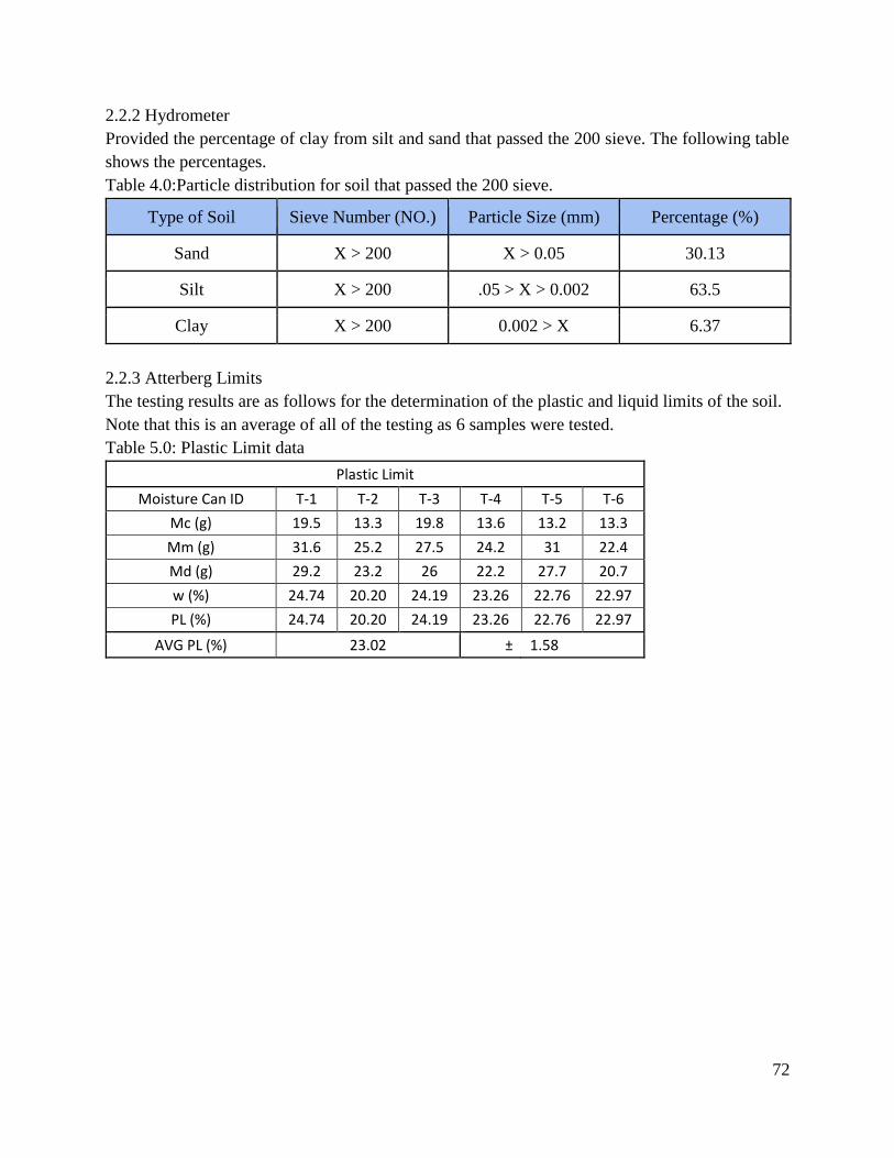
72
2.2.2 Hydrometer
Provided the percentage of clay from silt and sand that passed the 200 sieve. The following table
shows the percentages.
Table 4.0:Particle distribution for soil that passed the 200 sieve.
Type of Soil Sieve Number (NO.) Particle Size (mm) Percentage (%)
Sand X > 200 X > 0.05 30.13
Silt X > 200 .05 > X > 0.002 63.5
Clay X > 200 0.002 > X 6.37
2.2.3 Atterberg Limits
The testing results are as follows for the determination of the plastic and liquid limits of the soil.
Note that this is an average of all of the testing as 6 samples were tested.
Table 5.0: Plastic Limit data
Plastic Limit
Moisture Can ID T-1 T-2 T-3 T-4 T-5 T-6
Mc (g) 19.5 13.3 19.8 13.6 13.2 13.3
Mm (g) 31.6 25.2 27.5 24.2 31 22.4
Md (g) 29.2 23.2 26 22.2 27.7 20.7
w (%) 24.74 20.20 24.19 23.26 22.76 22.97
PL (%) 24.74 20.20 24.19 23.26 22.76 22.97
AVG PL (%) 23.02 ± 1.58

73
Figure 3.0 Liquid Limit Data
Liquid Limit- 24.92
Plastic Limit- 23.02
Cu- 12.11
Cc- 1.169
To classify the fill soil on the parcel, all methods were used to give a better understanding of the
soil. AASHTO, USCS, and USDA are shown with classification and soil descriptions.
Table 6.0: Soil Classification Summary
Classification Method Classification Description Soil Description
AASHTO A-1-b , A-3 Gravel Sand/ Fine Sand
USCS ML, SW Welly Graded Sand with Gravel
USDA N/A Sand
2.2.4 Triaxial
Testing is for the determination of the bearing capacity of the soil. Note that this is not being used
in the determination of the soil or the bearing capacity as testing did not provide sufficient data.
The actual The direct shear test will be done instead to determine the bearing capacity of the soil.
Results for the triaxial test are shown in Appendix F. The
y = -0.1128x + 27.372
20
21
22
23
24
25
26
27
28
29
10 15 20 25 30 35 40 45 50
Mo
uis
ture
Co
nte
nt
(%)
Number of Drops
Liquid Limit (LL)
T-1
T-2
T-3
T-4
T-5
T-6
Average
LL
LL
Linear (T-1)
Linear (T-2)
Linear (T-3)
Linear (T-4)
Linear (T-5)
Linear (T-6)

74
Figure 4.0: Triaxial Test Data
2.2.5 Proctor Compaction
The proctor compaction test provided a unit weight for the samples as shown in the table below.
This also was averaged to provide an optimal unit weight of 1752 Kg/m^3 at the peak of the curve
provided in Appendix E. The following are the results of the testing.
Figure 5.0: Modified Proctor Compaction Data
1550.0
1600.0
1650.0
1700.0
1750.0
1800.0
1850.0
0.000 0.050 0.100 0.150 0.200
Dry
Un
it W
eigh
t (k
N/m
^3
)
Moisture Content (g/g)
Modified Proctor Compaction
T-1
T-2
T-3
T-4
T-5
T-6
Average
Optimal
Optimal

75
2.2.6 Consolidation
Consolidation is used to determine the total settlement in the soil when a load is applied. The
following is the stress table that was collected from the consolidation testing that was completed.
Due to the lack of time and the amount of load on the soil. This was redone to collect accurate
results for settling. Unfortunately since the soil sample was disturbed, the results from this test are
inconclusive.
Table 7.0: Consolidation Test Data
Vertical Effective Stress (σ'z)=P/A
P A (σ'z)
4 kg 3231.0806 mm^2 0.00124 kg/mm^2
0.0032 m^2 1237.97592 kg/m^2
8 kg 3232.0806 mm^2 0.00248 kg/mm^2
0.0032 m^2 2475.95185 kg/m^2
16 kg 3233.0806 mm^2 0.00495 kg/mm^2
0.0032 m^2 4951.90370 kg/m^2
2.2.7 Direct Shear
Direct Shear was used to determine the friction angle of the soil. The data collected and plotted
in Figure 6.0 is the shear force applied on the soil against the horizontal displacement of the soil.
This data was used to create Figure 7.0 and allowed the friction angle to be determined.
Figure 6.0: Direct Shear Data
0
50
100
150
200
250
300
350
0 20 40 60 80 100 120
Shea
r F
orc
e (K
pa)
Horizontal Displacement (%)
Direct Shear
20kg
40kg
80kg

76
Figure 7.0: Friction Angle of soil
3.0 Summary of Analysis The soil that has been tested is from a fill that is located on the parcel. This is not a fully accurate
report as the soil that is on the site varies near the retaining wall. This will be used to design the
wall as parcel is mostly fill that is determined similar to the stockpile that the homogenous samples
were taken from. Soil sampling will continue as two more testing sessions are needed prior to wall
design.
The type of soil consists of mostly sand and small amounts of gravel and clay. This is ideal for the
design as the soil will have little to no settlement after the wall is completed. The soil is defined
as fine sand by the AASHTO standards. The amount of clay that the soil is negligible, however,
the consolidation test will determine if settlement is an issue due to the clay. The optimal dry unit
weight of the soil is 1752 kg/m^3 as the proctor compaction test identified. Triaxial did not provide
useable results and a direct shear test will be used in its place once completed for the bearing
capacity of the wall.
Overall, the soil will provide sufficient drainage and the soil is sufficient for the wall design as of
now. A further and more thorough report will be provided when the testing is finished.

77
Appendix D: Streamstats

78
Appendix D: Streamstats Results

79

80

81

82
Appendix E: Maricopa Standard Detail
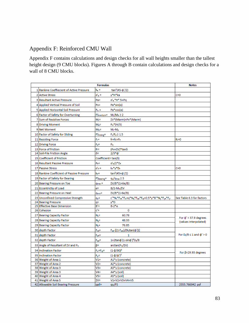
83
Appendix F: Reinforced CMU Wall
Appendix F contains calculations and design checks for all wall heights smaller than the tallest
height design (9 CMU blocks). Figures A through B contain calculations and design checks for a
wall of 8 CMU blocks.
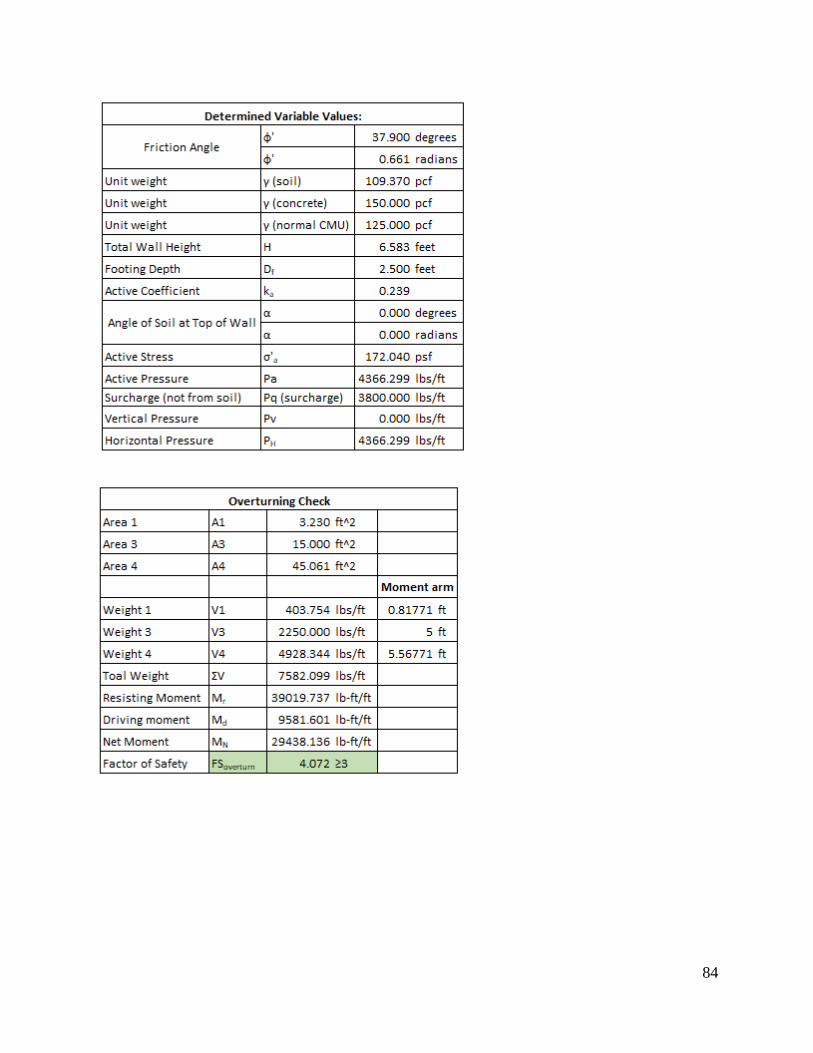
84

85

86
Figures C through D contain calculations and design checks for a wall of 7 CMU blocks.

87

88

89
Figures E through F contain calculations and design checks for a wall of 6 CMU blocks.

90

91
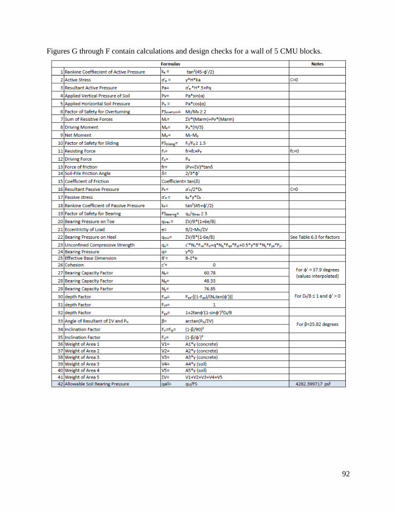
92
Figures G through F contain calculations and design checks for a wall of 5 CMU blocks.

93

94


![Second Thoughts[486]](https://static.fdocuments.in/doc/165x107/577d35651a28ab3a6b9052b5/second-thoughts486.jpg)