Cellular Automaton experiments on local galactic structure ...
18
ASTRONOMY & ASTROPHYSICS OCTOBER II 1996, PAGE 231 SUPPLEMENT SERIES Astron. Astrophys. Suppl. Ser. 119, 231-248 (1996) Cellular Automaton experiments on local galactic structure. I. Model assumptions J. Perdang 1 and A. Lejeune 2 1 Institute of Astronomy, Madingley Road, Cambridge CB3 OHA, UK, and Institut d’Astrophysique, 5, Avenue de Cointe, B–4000 Li` ege, Belgium ? 2 Institut de Physique, Sart–Tilman, B–4000, Li` ege, Belgium Received October 27, 1994; accepted March 6, 1996 Abstract. — The purpose of the present paper, combined with the companion paper (Lejeune & Perdang 1995, hereinafter Paper II), is to demonstrate that a Cellular Automaton (CA) framework incorporating detailed physical evolutionary mechanisms of the galactic components provides a straightforward approach for simulating local struc- tural features in galaxies (such as those of flocculent spiral galaxies). Conversely, and more important, the observed local irregularities may give information on the relevant timescales of the evolutionary processes operating in these galaxies. In this paper we start out with a critical review of the more standard methods in use in galactic modelling. We insist on the fact that these models do not lend themselves to a straightforward inclusion of both the galactic dynamics and the physical evolution of the galactic components. We show that the Cellular Automaton approach can combine both effects, on condition that the dynamics is approximated by a stationary, in general space–dependent velocity field of the galactic matter. The main part of the paper addresses an extension of the Stochastic Propagating Star Formation scheme originally devised by Mueller & Arnett (1976). The model consists in a multi–state 2D CA specifically designed to deal with the evolutionary behaviour of an off-centre region of a galaxy, of an area of a few kpc 2 . The model incorporates a detailed sequence of in part parametrised stellar evolutionary processes. In the version discussed here it includes as dynamical effects the motions of galactic matter due to a stationary circulation and, to some extent, due to the proper motions of the stars. The model we present is a first nontrivial instance of a CA de- fined over a lattice lacking geometric symmetries (crystal symmetries of standard CA, or rotational symmetry of the Mueller–Arnett CA). The precise geometry of the CA network of cells is imposed in our model by the space–dependent stationary galactic velocity field. Numerical results are discussed in the companion paper. Key words: galaxies: structure — star formation — methods: numerical 1. Introduction From the point of view of the formal theory of dynamical systems (DS), current galactic models belong into three broad categories. 1.1. Low order differential models On the one end of the spectrum of models, we have a class of elementary DSs, namely ordinary differential equations (ODEs) of low order (say n = 3, 4, ...). Such models are adopted to supply a theoretical basis for an understanding of the gross evolutionary behaviour of the local stellar con- tent, together with the chemical evolution of the galaxy. The formulation, dealing with a local part of the galaxy only, is reminiscent of chemical kinetics in a homoge- Send offprint requests to: J. Perdang ? Permanent address neous medium (Kaufman 1979; Shore 1981, 1982; Cowie & Rybicki 1982; Franco & Shore 1984; Shore et al. 1987; cf. also comments in Shore 1985). The counterparts of the chemical species are here the galactic species (interstellar gas and dust, and different classes of stars); the rates of the transformation processes of one species into another typically involve adjustable parameters. The main virtue of these models is that they demonstrate the important role of nonlinear steps in the evolution equations: Through nonlinear feedback the evolution may exhibit generically oscillatory as well as more complex stationary fluctua- tions, while a purely linear dynamics would imply an asymptotic evolution towards a time–independent state. Being of low order, the ODE formulations lend themselves to a more detailed mathematical analysis (Shore 1985). For n ≥ 2 these models have parameter ranges over which the evolutionary behaviour is periodic; for n ≥ 3 they may in principle exhibit deterministic chaos over some range,
Transcript of Cellular Automaton experiments on local galactic structure ...
ASTRONOMY & ASTROPHYSICS OCTOBER II 1996, PAGE 231
SUPPLEMENT SERIES
Astron. Astrophys. Suppl. Ser. 119, 231-248 (1996)
Cellular Automaton experiments on local galactic structure.
I. Model assumptions
J. Perdang1 and A. Lejeune2
1 Institute of Astronomy, Madingley Road, Cambridge CB3 OHA, UK, and Institut d’Astrophysique, 5, Avenue deCointe, B–4000 Liege, Belgium?
2 Institut de Physique, Sart–Tilman, B–4000, Liege, Belgium
Received October 27, 1994; accepted March 6, 1996
Abstract. — The purpose of the present paper, combined with the companion paper (Lejeune & Perdang 1995,hereinafter Paper II), is to demonstrate that a Cellular Automaton (CA) framework incorporating detailed physicalevolutionary mechanisms of the galactic components provides a straightforward approach for simulating local struc-tural features in galaxies (such as those of flocculent spiral galaxies). Conversely, and more important, the observedlocal irregularities may give information on the relevant timescales of the evolutionary processes operating in thesegalaxies. In this paper we start out with a critical review of the more standard methods in use in galactic modelling.We insist on the fact that these models do not lend themselves to a straightforward inclusion of both the galacticdynamics and the physical evolution of the galactic components. We show that the Cellular Automaton approach cancombine both effects, on condition that the dynamics is approximated by a stationary, in general space–dependentvelocity field of the galactic matter. The main part of the paper addresses an extension of the Stochastic PropagatingStar Formation scheme originally devised by Mueller & Arnett (1976). The model consists in a multi–state 2D CAspecifically designed to deal with the evolutionary behaviour of an off-centre region of a galaxy, of an area of a fewkpc2. The model incorporates a detailed sequence of in part parametrised stellar evolutionary processes. In the versiondiscussed here it includes as dynamical effects the motions of galactic matter due to a stationary circulation and, tosome extent, due to the proper motions of the stars. The model we present is a first nontrivial instance of a CA de-fined over a lattice lacking geometric symmetries (crystal symmetries of standard CA, or rotational symmetry of theMueller–Arnett CA). The precise geometry of the CA network of cells is imposed in our model by the space–dependentstationary galactic velocity field. Numerical results are discussed in the companion paper.
Key words: galaxies: structure — star formation — methods: numerical
1. Introduction
From the point of view of the formal theory of dynamicalsystems (DS), current galactic models belong into threebroad categories.
1.1. Low order differential models
On the one end of the spectrum of models, we have a classof elementary DSs, namely ordinary differential equations(ODEs) of low order (say n = 3, 4, ...). Such models areadopted to supply a theoretical basis for an understandingof the gross evolutionary behaviour of the local stellar con-tent, together with the chemical evolution of the galaxy.The formulation, dealing with a local part of the galaxyonly, is reminiscent of chemical kinetics in a homoge-
Send offprint requests to: J. Perdang?Permanent address
neous medium (Kaufman 1979; Shore 1981, 1982; Cowie &Rybicki 1982; Franco & Shore 1984; Shore et al. 1987; cf.also comments in Shore 1985). The counterparts of thechemical species are here the galactic species (interstellargas and dust, and different classes of stars); the rates ofthe transformation processes of one species into anothertypically involve adjustable parameters. The main virtueof these models is that they demonstrate the importantrole of nonlinear steps in the evolution equations: Throughnonlinear feedback the evolution may exhibit genericallyoscillatory as well as more complex stationary fluctua-tions, while a purely linear dynamics would imply anasymptotic evolution towards a time–independent state.Being of low order, the ODE formulations lend themselvesto a more detailed mathematical analysis (Shore 1985).For n ≥ 2 these models have parameter ranges over whichthe evolutionary behaviour is periodic; for n ≥ 3 they mayin principle exhibit deterministic chaos over some range,
232 J. Perdang and A. Lejeune: Cellular Automaton experiments on local galactic structure. I.
although such a behaviour has not yet been reported sofar. By ignoring spatial exchanges — diffusion in the ana-logue of chemical kinetics — such models automaticallydiscard, to a large extent, the details of the interactionsbetween different species.
In spite of their simplicity, these models may also pro-duce nontrivial space patterns: If the local transformationrates include a slight systematic radial space dependence,then in a periodic regime the ensuing space dependenceof the period is responsible for the formation of annularisodensity lines of the different constituents (cf. Perdang1974); the kinematics of rotation is then sufficient to de-form the latter into spirals.1
Within this class of models global mechanical effects,such as galactic rotation and gravitation, are entirely ig-nored.
1.2. High order differential models
At the other end of the spectrum of galactic models wehave a class of DSs in the form of ODEs of high or-der (> 103), namely N–body simulations. Following theinitial attempts of the late 60’s (Miller & Prendergast1968; Hockney & Hohl 1969; cf. also Aarseth 1972), theseoriginally 2D models incorporate as only physics gravi-tation (combined with rotation through appropriate ini-tial conditions). In principle, these models cope there-fore with the correct global galactic mechanics, thougheven the most accurate N–body programs, handling some106−107 bodies, work at a numerical ‘noise level ... aboutone thousand times higher than ... a galaxy’ (Sellwood &Wilkinson 1993). N–body calculations generate spatialinhomogeneities: With simplest initial conditions for agalaxy (statistically uniform density; systematic rotationwith superposed random motions of the individual bodies;absence of a halo), these experiments produce a (transient)double arm connected by a central bar (cf. the original 2Dexperiments by Hohl 1971), or more generally, coherentspatial matter concentrations reminiscent of spiral armsand bars (cf. the 3D experiments by Raha et al. 1991;and the analysis by Pfenniger & Friedli 1991).
N–body models are predicated on the assumption thatthe constituents are structureless permanent point masses;the intrinsic physical evolution of the individual galac-tic species is ignored. On the other hand, the prominentglobal observational structures in a galaxy, such as thegeometry of a spiral arm or of a central bar, are of an ‘op-tical’ nature. The observed geometry is the geometry ofthe isophotes; any photometric or photographic techniquesupplies a brightness map, rather than a direct picture
1If diffusion is superimposed on the chemical kinetic equa-tions — transforming the elementary DS into a different classof a DS, namely a system of partial differential equations(PDEs) —, the oscillating regime gives rise to travelling waveswhich again can form spiral patterns (Cowie & Rybicki 1982;Feitzinger 1985).
of hydromechanical properties (such as the distributionof matter density). While the statement “ ‘brightness’ re-quires the ‘presence of matter’ ”, is manifestly true, theconverse statement “ ‘presence of matter’ implies ‘opticalobservability’ ”, does not hold. Any inferences on the mat-ter distribution from optical observations (including radio,cm, mm, IR, UV, X and gamma) are indirect, and neces-sarily based on disputable, and disputed, assumptions onthe chemical nature and the physical state of the galacticmatter.
High luminosity in optical light, on the other hand,is chiefly the result of the presence of stars in their ear-liest evolutionary phases. It is then not obvious to con-ceive that purely mechanical N–body models, interestingas they may be, should satisfactorily account for an inter-pretation of the salient brightness patterns of galaxies asshown for instance in blue light photographs.
1.2.1. The problem of reduction of the order
On the mathematical side, the high order n (= 6N in3D experiments) of the ODEs representative for N–bodymodels constitutes a major hurdle to a theoretical investi-gation of the allowed time and associated space behaviourof these DSs. Accordingly our knowledge of the dynam-ics of these models mainly rests on numerical experimen-tation, even though ad hoc approximation schemes mayprovide clues towards interpreting the results. Thus thesubstitution to the instantaneous N–body potential of asmoothed out stationary potential decouples the mass–points, and lends itself to an analysis and classification ofthe allowed orbits (cf. Binney & Tremaine 1987 Chapt.3; cf. de Zeeuw & Franx 1991 for comments on modelsfor elliptical galaxies); in this context, the observation ofbars in the N–body experiments may be attributed tothe existence of ‘box orbits’ in the mean potential ap-proximation. The method devised by Schwarzschild (1979,1982) is a refinement of this approach, in which a self–consistent smoothed stationary potential is numericallygenerated from a large collection of trial orbits, via an it-erative technique. A more pragmatic method is adoptedby Contopoulos and coworkers (Patsis et al. 1991); theseauthors relate the smoothed stationary potential (with su-perposed spiral perturbation) to a parametrised analyticalinterpolation formula of the rotation curve of a galaxy; thefree parameters are then observationally fitted; the den-sity structure of the galaxy is finally simulated using alarge enough sample of computed orbits.
Models of this type have been successful in reproducingthe spatial distribution of the molecular gas (simulated astest particles; cf. for instance Sempere et al. 1995 in thecase of M100).
It is true that very often dynamical systems with largenumbers of degrees of freedom asymptotically relax ona short timescale to an internal equilibrium in which a
J. Perdang and A. Lejeune: Cellular Automaton experiments on local galactic structure. I. 233
substantial fraction of the actual degrees of freedom ceaseto participate in the dynamics.2
Under those conditions, once an internal equilibrium isestablished, the physically relevant evolution depends ef-fectively on the small number of order parameters alone,which in turn obey the dynamics of a low order ODE.A mean potential representation, to the extent that it isan asymptotically correct description of the N–body be-haviour, may perhaps be justified on the basis of this gen-eral observation.
A systematic, and mathematically precise methodthat achieves the reduction of degrees of freedom is thePoincare Normal Form technique (cf. Arnold 1976). Thistechnique demonstrates that a reduction to a low orderof the originally high order ODEs representative for thenumerical treatment of the dynamics of a star is not al-lowed in the general 3D case (while such a reduction doeshold if the dynamics is forced to be strictly radial): in the3D case the reduced ODE remains of a very high order(Perdang 1994). Due to a formal similarity of the equa-tions of stellar and galactic dynamics, we may infer thatthe stellar non–reducibility should extend to the case ofgalactic structure. Simplified models, such as the mean po-tential approach, may supply partial information on lim-ited sub–problems; to understand the general aspects ofthe N–body dynamics, however, actual large scale numer-ical experiments appear as inevitable.
1.2.2. The fluid dynamic approach
A macroscopic variant of the microscopic N–body equa-tions is a formalism of fluid dynamics as derived froma Boltzmann (Vlasov) equation approach. The formula-tion of fluid dynamics belongs into a new category of DSs,namely partial differential equations (PDEs). Although re-lying on a spatial smoothing of the microscopic dynamics,the macroscopic PDE formulation preserves the large (for-mally infinite) number of degrees of freedom. It is there-fore not subject to the above criticism and can serve thepurpose of interpreting the global behaviour of N–bodyexperiments.
Linear stability calculations of differentially rotatingdiscs initiated by Lin & Shu (1964, 1966; also Lin 1966)in the context of this model demonstrate the existence ofunstable modes. The density pattern of the most unsta-ble mode, reminiscent of the observed structure of spiralarms, is then identified with the global spiral structure— the Grand Design of Sa, Sb and Sc galaxies — (cf.Shu 1991 Chapt. 11; Bertin et al. 1989; cf. also Binney& Tremaine 1987 chapt. 6) as well as with the matter
2More precisely, in the terminology of Haken, a large numberof the actual degrees of freedom are ‘slaved’ by a few relevantdegrees of freedom, or ‘order parameters’ (Haken 1977 chapt.7). The latter collective degrees of freedom alone eventuallygovern the macroscopic time behaviour.
concentrations as traced in the N–body experiments; thisconjecture is the main ingredient of the density wave the-ory. Although actual calculations are limited to the linearregime, a physical argument (nonlinear stabilisation of thelinearly unstable mode as a result of dissipation leadingto a stationary finite amplitude pattern; Kalnajs 1972)suggests that the global pattern is the outcome of a sin-gle symmetry–breaking in the uniform disc induced by adynamic instability.3
Theoretically it is not obvious why the geometricallysmooth linearly unstable pattern should preserve its in-cipient shape in a nonlinear regime. Nothing excludes apriori the occurrence of a hierarchy of superposed sym-metry breakings away from the regular stationary armpattern; this hierarchical scenario would in turn lead toincreasingly less trivial stationary as well as nonstation-ary geometries. We recall in this connection that Couette–Taylor flow, not unrelated to the large scale flow set upin a rotating galaxy, is indeed subject to a variety ofsymmetry–breaking instabilities, as is known both the-oretically and experimentally (Brandstadter & Swinney1987; Cross & Hohenberg 1993). Likewise, the geometry ofa hydrodynamic vortex exhibits an irregular spiral patternreminiscent of spiral galaxies (cf. the vortex simulations inLavallee et al. 1993).
Finally, even in the case of the geometrically most reg-ular galaxies the observed structure of the galactic armsdoes not really exhibit the smooth and regular shape ofthe unstable linear density waves (cf. M81 chosen in King1989a to demonstrate the Grand Design; cf. in particularthe plates pp. 99-105, 119-127 in the Revised Shapley–Ames Catalog, Sandage & Tamman 1981 (RSAC), andthe large scale plates (Part II) in the Atlas of Galaxies,Sandage & Bedke 1988 (AG)).
Besides these weaknesses proper to the linear densitywave theory, any fluid dynamic approach — or nonlin-ear wave theory — shares what we believe is the majorweakness of the N–body model which it is meant to re-produce: Like the latter, it ignores any evolutionary ef-fect in the individual galactic species. On the other hand,the fluid dynamic approach may remain meaningful fordealing with the interstellar gas. Regarding the interstel-lar medium, the atomic component is typically observedvia HI in the Milky Way (since 1951, 21 cm line); as atracer of the molecular component, in particular of the gi-ant molecular clouds (GMC), and hence of the regions ofstar formation, CO is used (1.3 and 2.6 mm line; cf. King
3A symmetry–breaking from an original axisymmetry (C∞group) necessarily consists in a transition to a subgroup ofthe latter, i.e. to some Cm ⊂ C∞ (m–fold rotational symme-try), regardless of the physics involved; representatives of Cmare m–fold arms. The specific selection m = 2 as already ex-hibited in Hohl’s (1971) N–body experiments — and in realgalaxies — depends on the precise physics responsible for theinstability.
234 J. Perdang and A. Lejeune: Cellular Automaton experiments on local galactic structure. I.
1989; Combes 1991). As is convincingly demonstrated bya comparison of a plot of the HI column density bright-ness in M81 (Fig. 6-23 in Binney & Tremaine 1987) with ablue–light photograph of this galaxy (p. 123 in the RSAC),the HI distribution globally follows the arms of the pho-tograph, even though the two specific geometries are notidentical (see also Fig. 10.8 in van der Kruit 1989, showinga similar situation for NGC 628). Maps of the CO distribu-tion in M51 compared with various other maps (HI, Hα)exhibit elongated patches sketching the global shapes ofragged arms; the arm structures of CO, HI and Hα areagain roughly, though not exactly, coincident (cf. Fig. 3 inYoung & Scoville 1991).
1.3. Cellular Automaton models
As a category of galactic structure DSs not encoded inconventional ODEs or PDEs, a novel methodology wasintroduced in the 70s, in the form of cellular automatonmodels. With a discretised time, a discretised space (2D inthe majority of models devised so far), and with a discreterepresentation of the physics, the dynamics of the CA iscaptured algebraically by an iteration in the integral do-main of the integers (a system of a large number [> 105]of difference equations in integer variables). The latter cantherefore be solved exactly. This is a major computationaladvantage of a CA model over ODE and PDE formulationswhose numerical solutions are always subject to round–offerrors: Instabilities, especially multiple competing insta-bilities, are hard to control in an ODE or PDE frameworkwhere round–off errors are then amplified exponentiallyin time. Since, as stressed above, such instabilities are notunlikely to occur in real galaxies, we believe that the CAenvironment is a computationally more satisfying frame-work for galactic modelling.
As a further advantage of the CA framework for han-dling physics, we point out that physical mechanisms hardto translate into ODE or PDE form are often trivially ex-pressed as CA rules (cf. the discussion in Perdang 1993).4
4An illustration is the chaotic mechanism for the formationof irregular structure as suggested by Goldreich & Lynden–Bell (1965) and which so far remained on a descriptive level.According to Elmegreen & Elmegreen (1982) about 70% ofthe isolated spiral galaxies are flocculent; they exhibit ‘short,chaotic–looking arms and no apparent symmetry’ (Elmegreen& Elmegreen 1983). To account for the raggedness and patch-iness of real galactic arms Goldreich and Lynden–Bell proposethe following scenario: Through a spontaneous Jeans instabil-ity in a clump at some random location in the galaxy and atsome random instant of time, a nest of protostars is created.The kinematic shearing effect of the differential rotation subse-quently stretches this aggregate of young objects into an elon-gated, irregular patch — a local portion of a luminous arm. Dueto the short lifetime of the high luminosity phase of the youngstars, the actual visibility of such a localised arm structure isseverely limited in time. An impression of a global continuous
The first attempt at simulating the global morphologyof spiral galaxies in the framework of a CA model was dueto Mueller & Arnett (MA) (1976). The CA formulationwas carried further in a series of papers by Gerola, Seiden,Schulman and coworkers (GSS) (Gerola & Seiden 1978;Seiden et al. 1979, 1982; Seiden & Gerola 1979; Gerola etal. 1980; Schulman & Seiden 1982; for discussions and ex-tended reviews see Seiden & Gerola 1982; Schulman & Sei-den 1983, 1986; Seiden & Schulman 1990; Schulman 1993),as well as by Comins & coworkers (C) (Comins 1981, 1983,1984; Statler et al. 1983; Balser & Comins 1988; Comins& Shore 1990). Essentially, a galactic CA model may in-corporate any physical ingredient of the low-dimensionalODE models listed under (1), with an additional imple-mentation of space dependence.
The simplest CA version is based on 4 physical as-sumptions and approximations:
(a) The model incorporates two galactic species only,namely ‘gas’ or ‘dust’, D, and ‘stars’, S (in the form ofluminous high mass stars); each cell of the automaton iseither in the D state, or in the S state.
(b) The model takes account of the kinetics of the ob-servationally documented processes of star formation in aparametrised form. These mechanisms are:
(α) spontaneous star formation, viewed as any processconforming to a decay reaction
D → S; (1.1)
a cell in state D spontaneously transforms into a stateS with a given probability per timestep (simulation of aspontaneous Jeans instability of the interstellar medium);and
(β) star–induced star formation, or self–propagatingstar–formation (SPSF) in the terminology of MA; formallySPSF refers to the totality of autocatalytic processes obey-ing a stoichiometric scheme
D + m S → (1 +m) S; (1.2)
a cell in state D transforms into a state S with a givenprobability per timestep provided that there are m cellsin state S in the neighbourhood. This step accounts forthe observational evidence of star formation (presence ofOB associations) in expanding spherical shells surround-ing supernovae and high luminosity stars in general (San-cisi 1973; Berkhuijsen 1974; Castor et al. 1975; Elmegreen& Lada 1977); these observations are interpreted as the ef-fects of shocks generated by supernova explosions (Arnettet al. 1989), shocks associated with H–ionisation fronts
spiral arm pattern is eventually created by the simultaneouspresence of a large number of such short–lived elongated lumi-nous patches appearing and disappearing at random positions;the overall shape of the arm reflects the direction of the stretch-ing. It is not clear how this mechanism could be captured bya PDE model; on the other hand the CA framework describedbelow incorporates the mechanism automatically.
J. Perdang and A. Lejeune: Cellular Automaton experiments on local galactic structure. I. 235
due to OB stars (Elmegreen & Lada 1977, who quote M42,M17, M8, NGC 7538), or shocks connected with stellarwinds generated by massive stars. These shocks compressthe interstellar gas into molecular clouds, or the clumpsin a cloud, which in turn transform into stars.5
(c) The standard CA model incorporates a station-ary circular differential rotation of the galaxy (cells arearranged in rings which are rotated at different speeds,in accordance with a given rotation law). Rotation thusplays a kinematic role only, thereby influencing howeverthe processes of star formation. Gravitation is not explic-itly handled in this CA version; this should not be equatedwith saying that gravitation is just ignored. The station-ary kinematic motion which is implemented is to be inter-preted dynamically as resulting from all forces — includ-ing gravitation — acting on the galactic matter. Althoughan improvement over the ODE models (1), assumption (c)corresponds to a lower order approximation of the galac-tic dynamics than the mean potential method mentionedunder (2): Stationary rotation amounts to taking accountof the simplest class of dynamically allowed orbits only,namely circular orbits in a mean radial gravitational field;moreover, the possible occurrence of resonances — andthe possibility of chaotic dynamics — is ignored. The av-eraged potential models under (2) sample in principle allcategories of allowed orbits including chaotic dynamicalbehaviour.
(d) Initially all cells are in the (‘active’) D state.
If spatial structure emerges in this model, then it isnot due to a direct action of gravitation on matter; thiscontrasts with models (2), in which the wave pattern isrelated exclusively to the inhomogeneities in the matterdensity. In a CA model obeying the kinematic assump-tion (c) the originally uniform overall density distribution(assumption (d)) is preserved; structure can only arise asa consequence of the evolution of the galactic components(asumption (b), Eqs. (1.1) and (1.2)); the global motionand hence indirectly gravitation modulate however thelocal rates of these evolutionary processes. The develop-
5In the context of the CA models of GSS the simulationparametrises the rates of the ‘chemical reactions’ (1.1) and(1.2). To the extent that the star formation mechanisms con-form to these reactions, the simulation remains invariant underany specific interpretation of the two mechanisms. It is irrel-evant whether it is a real shock or any other physical process(for instance a gravitational interaction, or some other energytransfer) that induces the transformation of gas into stars inprocess (1.2), provided only that this process requires the pres-ence of nearby stars. In GSS the gas component D is subdi-vided into an ‘active’ and an ‘inactive’ phase parametrised by a‘refractory time’ τ . Essentially, if a star formation event has oc-curred in a given cell at a given time, then during τ timestepsthis same cell remains ‘inactive’ in the sense that if it con-tains gas then the latter is not allowed to transform into stars.We observe in passing that the refractory time is a parameterwhich is hard to estimate physically.
ment of a pattern corresponds to a spatial organisationof the two galactic components, rather than to a globalrearrangement of matter density (as happens in models(2)).
It was recognised by MA that it was the specific SPSFmechanism — the autocatalytic step (1.2), i.e. the pres-ence of a nonlinear fragment in the ‘reaction kinetics’ —which was eventually responsible for the development ofa chain of contiguous active cells interpreted as the lumi-nous galactic arm. Schulman and coworkers subsequentlyidentified the formation of the arm pattern with a per-colation phenomenon in the star population (modified bythe galactic kinematics; cf. Schulman & Seiden 1983, andSeiden & Schulman 1990 for analytical details). If allmodel parameters except the probability of induced starformation, p (process 1.2), are kept fixed, then the corre-lation length of the star population, ξ(p), and the meancluster size of the star population (total number of stars ina group of stars occupying contiguous cells), S(p), divergeas
ξ(p) ∼ | pc − p |−ν (a), and S(p) ∼ | pc − p |−γ (b),(1.3)
as the free parameter p approaches a critical value pc (cf.Stauffer 1985). Given the geometry of the cellular grid ofthe CA, the critical exponents ν, γ (> 0) can be estimatedtheoretically. For a probability p < pc the catalytic process(1.2) remains too inefficient to secure the actual propaga-tion of star formation; there will be no unbounded clusterof activity. A huge cluster of stellar activity — a galacticarm — is formed at the percolation phase transition whenp tends to pc (S(p) →∞).6
Even these simplest CA schemes have been surpris-ingly successful in generating synthethic pictures of galax-ies which closely resemble photographs of real galaxies (cf.the comparisons of CA simulations with the blue plates ofNGC 628 [Sc(s)I in the classification scheme of the RSAC]and NGC 7793 [Sd(s)IV] in Schulman & Seiden 1986, orSeiden & Schulman 1990). Photographs of real galaxies arein fact far better mimicked by CA simulations than by thecomputationally much more involved full N–body simu-lations (cf. for instance Sellwood & Carlberg 1984) or ap-proximate many–body simulations in given gravitationalfields (possibly modified by self–gravitational effects;cf. the simulations of molecular cloud distributions inSempere et al. 1995). Whatever the critique directed
6To secure the actual realisation of a proper galactic arm pat-tern a further condition must be satisfied. If the reaction proba-bility exceeds a second critical value pM (> pc) then essentiallyall matter is in the active star state and the configuration isuniformly luminous; there are no individual arms (cf. in partic-ular the survey in C 1981). Accordingly, in order to guaranteethe formation of a realistic arm pattern, the probability pa-rameter p must be confined to some interval (pc, pM).
236 J. Perdang and A. Lejeune: Cellular Automaton experiments on local galactic structure. I.
against the admittedly elementary, and incomplete, na-ture of this CA model, its success in duplicating real pho-tographs of galaxies secures that it deserves credit, at leastas a tool of heuristic value and efficacy.
Reviews of spiral structure theory characteristicallypresent the density wave scheme and the SPSF CA astwo rival theories designed to interpret the formation andthe stability of galactic arms (cf. Shu 1985). In the formermodel gravitation coupled with rotation is responsible fora mechanical (second order) phase transition from spa-tial homogeneity to spatial structure in the global matterdistribution. In the latter model, the change in the mor-phology leaves the global matter distribution essentiallyunaffected; structure results from inhomogeneities in thespace distribution of the galactic components created ina percolation–like phase transition caused by the SPSFmechanism, and modulated by the galactic mechanics.
Since both dynamics and catalytic star formation pro-cesses coexist in real galaxies, the two instability mecha-nisms, rather than being antagonistic, are complementary,and they may well be operative simultaneously. This be-lief was already expressed by MA who suggested that theSPSF effect might be responsible for the more ‘irregularoptical appearance often seen in late–type spiral galaxies’,while the classic symmetric two–arm spirals might be ofgravo–rotational origin. The same idea has been repeatedmore recently by Schulman (1993, p. 312) who argues that‘some [galaxies] are dominated by gravitational and fluiddynamic effects, while for others the morphology is a con-sequence of the statistical mechanics effects’ as capturedin the CA model.
If it is true that the morphology is at least to someextent determined by the SPSF effect, and, more gener-ally, by evolutionary effects of the galactic components(gas, different species of stars, ...), then we are entitled toexpect that in turn the morphology may supply informa-tion on the evolutionary processes of these components.It is this ‘inverse problem’ which motivates our interestin concentrating on a more detailed physical model of theinternal evolution.
2. The adopted methodology
In view of the above remarks, a satisfactory galactic modelshould incorporate both instability mechanisms, the dy-namical density wave effect and the SPSF process. In prin-ciple, this could be achieved either in the context of modelsof category (2), by superposing stellar formation and evo-lution on an already time–consuming mechanical N–bodyproblem (or on the averaged potential variant thereof);or, in the framework of models of category (3), by explic-itly handling the galactic dynamics within a CA model.Unfortunately, neither procedure is easy to implement.
On the other hand, in a simulation of galaxies in whichthe flocculent character is well developed, we believe thatthe global mechanical effects play a relatively minor part
in determining the structure (cf. the comments of MA), sothat we are entitled to treat galactic mechanics as a ‘per-turbation’. We then propose the following hybrid methodwhich takes account of the specific advantages of both ap-proaches (2) and (3):
(a) The dynamics, in the form of the N–body problem(2), (or of a convenient approximation to the latter; cf.the mean stationary potential approximation), is solvedseparately; a hydrodynamic velocity field v(r, t) is thenderived by ensemble–averaging. Provided that the gener-ally accepted assumption of stationarity holds, the veloc-ity field v(r) may directly be determined observationally(cf. Fig. 6-23 in Binney & Tremaine 1987 showing v(r)in M81 as estimated from the HI distribution). The latterapproach was in fact followed by the first proponents ofthe SPSF model, with the further simplifying assumptionthat the stationary velocity field is purely rotational.
(b) The CA model is then run with the velocity fieldv(r, t) (or v(r)) as given in step (a) added as a kinematicconstraint. Under the theoretical alternative of (a), thesequence of steps (a) and (b) may be repeated until con-vergence.
A flexible technique for implementing an arbitraryspace–dependent stationary velocity field in a CA environ-ment consists in adopting a network of cells whose shapesand sizes are functions of position determined by the ve-locity field itself (cf. the discussion and illustration of thisprocedure in Perdang 1993); the specific details of thistechnique are discussed below. The method in the formadopted here appears to be a convenient strategy for adirect simulation of small parts of a galaxy. To model awhole galaxy, a variant of it which remains closer to thestandard CA implementation of a pure rotational veloc-ity field as adopted by previous authors (MA, GSS, C) isprobably more convenient (cf. below).
Besides our concern for improving the treatment of thegalactic dynamics in the CA modelling environment, thepresent work is motivated by several further observationaland theoretical points.
The large–scale plates of spiral galaxies in the AGdemonstrate that the geometry of the spiral pattern ofeven the most regular grand–design galaxies is not fullyconsistent with the geometrically smooth and regularshape of unstable density modes (cf. Binney & Tremaine1987, Chapt. 6.3). The observed patterns are alwaysragged and fragmented, exhibiting alternating high andlow brightness concentrations along an arm. The clear–cut geometry of a theoretical linear mode transpires onlyafter strongly smoothing and filtering the galaxy pictures.On the other hand, the actually observable small–scalestructure of the isophotes bears a visual similarity withthe isophotes of molecular clouds, suggesting in turn thatphysically similar mechanisms may be operative on thescale of the arms and on the scale of the clouds. Bazell& Desert (1988) who analysed the geometry of constant
J. Perdang and A. Lejeune: Cellular Automaton experiments on local galactic structure. I. 237
brightness contours of several molecular clouds (IRASSky Flux plates) reported fractal dimensions in the range1.12−1.40 for the latter; a morphological image analysisof the η Carinae cloud (ESO plate) by Blacher & Perdang(1990) led to fractal dimensions of different brightness lev-els in the range 1.33−1.45. We expect therefore that thecontours of the arm structure are characterised by fractaldimensions in a similar range, say 1.1−1.5.
Density wave theory in its elementary linear form isnot consistent with fractality of the arms. In a nonlinearvariant, density wave simulations based on averaged po-tentials do generate fractured irregular arms (especiallynear the 4/1 resonance; cf. the simulated photograph Fig.8b in Patsis et al. 1991); however, a mere visual compari-son of the shape of the simulated arms (cf. again Fig. 8bin Patsis et al. 1991) with the arms of real galaxies indi-cates morphological differences which are hard to quan-tify; moreover, it remains to be shown that the conjec-tured fractality of the simulations is not just an artifactof the low number of sampling orbits. In the frameworkof gravity–induced dynamics a full existence proof of atransition to fractality is lacking, although numerical ex-periments are not inconsistent with an evolution towardsa hierarchical gravitational organisation (cf. for instancethe 1D experiments in Rouet et al. 1991).7
In contrast, it is well known experimentally that in CAmodels fractal structures are common, and for a variety ofsimple CA evolution rules the occurrence of fractal (spaceor space–time) structures can be proved analytically (cf.Perdang 1993). We also recall that percolation clustershave fractal boundaries. Accordingly, a CA formulationseems to be an adequate framework for a study of theformation of a fractal arm morphology.
Besides a fractal geometry of the arm structure, a sec-ond type of spatial fractality is to be expected: It has beensuggested (Ikeuchi & Yoshioka 1989) that the supernovaremnants are fractally distributed in space, in the sensethat these objects uniformly cover a fractal region of thegalaxy. Since stellar evolutionary effects are not easily im-plemented in models of class (2), we adopt a CA formalismwhich can accommodate several stellar species without un-due computational complications. In the context of CAmodels it is a well known experimental fact that specificcellstates can obey fractal space distributions; moreover,for some simple CA evolution rules the existence of frac-
7The special equations of isothermal self–gravitating 2D fluiddynamics of radial symmetry (matter in an infinite circularcylinder), containing an ad hoc modification to deal with apossible fractal matter distribution, can be shown to be in-variant under a Lie group acting also on the dimension of thematter distribution; physically this result means that the sys-tem may be deformed without energy expenditure, and henceit may spontaneously evolve from an original non–fractal ge-ometry — the standard matter distribution in the cylinder —to a fractal geometry (Perdang 1995).
tal distributions can be shown analytically (cf. Perdang1993).
3. Geometry of the CA simulation
In contrast with the CA models as designed by MA, GSSand C, which deal with a global simulation of an entiregalaxy, the model we introduce here addresses the mor-phology of a small part of a galaxy only. It aims at simu-lating irregular luminous matter concentrations (irregulararm structures) in off–centre regions of intermediate typegalaxies (between extreme flocculent and grand–design).Specimens of such galaxies are M33 (arm class 5), or M100and M101 (arm class 9) (Elmegreen 1981).
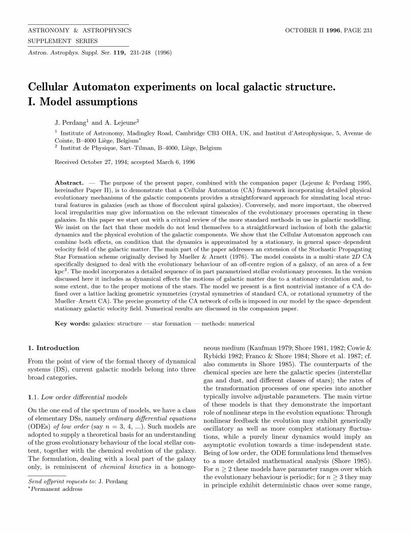
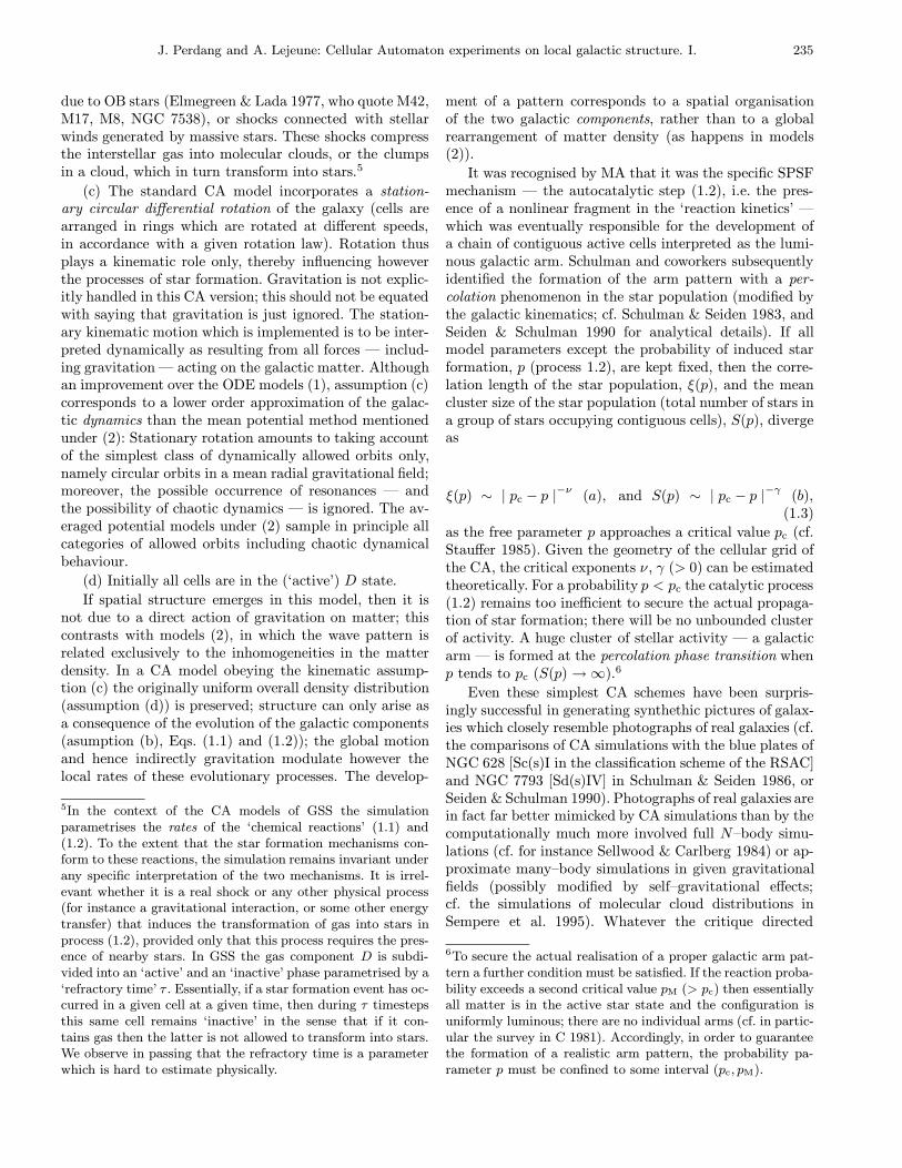
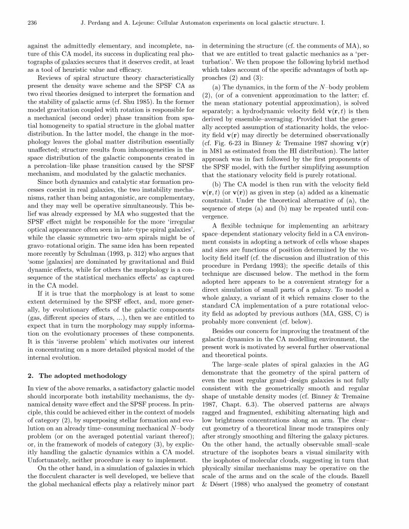
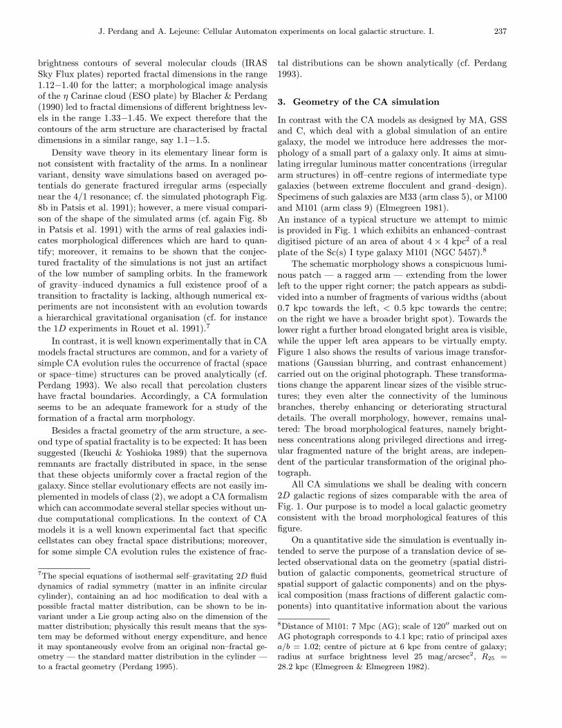
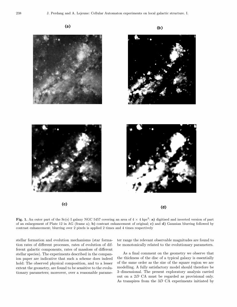
An instance of a typical structure we attempt to mimicis provided in Fig. 1 which exhibits an enhanced–contrastdigitised picture of an area of about 4 × 4 kpc2 of a realplate of the Sc(s) I type galaxy M101 (NGC 5457).8
The schematic morphology shows a conspicuous lumi-nous patch — a ragged arm — extending from the lowerleft to the upper right corner; the patch appears as subdi-vided into a number of fragments of various widths (about0.7 kpc towards the left, < 0.5 kpc towards the centre;on the right we have a broader bright spot). Towards thelower right a further broad elongated bright area is visible,while the upper left area appears to be virtually empty.Figure 1 also shows the results of various image transfor-mations (Gaussian blurring, and contrast enhancement)carried out on the original photograph. These transforma-tions change the apparent linear sizes of the visible struc-tures; they even alter the connectivity of the luminousbranches, thereby enhancing or deteriorating structuraldetails. The overall morphology, however, remains unal-tered: The broad morphological features, namely bright-ness concentrations along privileged directions and irreg-ular fragmented nature of the bright areas, are indepen-dent of the particular transformation of the original pho-tograph.
All CA simulations we shall be dealing with concern2D galactic regions of sizes comparable with the area ofFig. 1. Our purpose is to model a local galactic geometryconsistent with the broad morphological features of thisfigure.
On a quantitative side the simulation is eventually in-tended to serve the purpose of a translation device of se-lected observational data on the geometry (spatial distri-bution of galactic components, geometrical structure ofspatial support of galactic components) and on the phys-ical composition (mass fractions of different galactic com-ponents) into quantitative information about the various
8Distance of M101: 7 Mpc (AG); scale of 120′′ marked out onAG photograph corresponds to 4.1 kpc; ratio of principal axesa/b = 1.02; centre of picture at 6 kpc from centre of galaxy;radius at surface brightness level 25 mag/arcsec2, R25 =28.2 kpc (Elmegreen & Elmegreen 1982).
238 J. Perdang and A. Lejeune: Cellular Automaton experiments on local galactic structure. I.
Fig. 1. An outer part of the Sc(s) I galaxy NGC 5457 covering an area of 4 × 4 kpc2: a) digitised and inverted version of partof an enlargement of Plate 12 in AG (frame a); b) contrast enhancement of original; c) and d) Gaussian blurring followed bycontrast enhancement; blurring over 2 pixels is applied 2 times and 4 times respectively
stellar formation and evolution mechanisms (star forma-tion rates of different processes, rates of evolution of dif-ferent galactic components, rates of massloss of differentstellar species). The experiments described in the compan-ion paper are indicative that such a scheme does indeedhold: The observed physical composition, and to a lesserextent the geometry, are found to be sensitive to the evolu-tionary parameters; moreover, over a reasonable parame-
ter range the relevant observable magnitudes are found tobe monotonically related to the evolutionary parameters.
As a final comment on the geometry we observe thatthe thickness of the disc of a typical galaxy is essentiallyof the same order as the size of the square region we aremodelling. A fully satisfactory model should therefore be3–dimensional. The present exploratory analysis carriedout on a 2D CA must be regarded as provisional only.As transpires from the 3D CA experiments initiated by
J. Perdang and A. Lejeune: Cellular Automaton experiments on local galactic structure. I. 239
Comins (1983; Statler et al. 1983), the inclusion of thethird dimension may indeed alter the quantitative conclu-sions drawn from 2D simulations.
4. Dynamics of the CA simulation
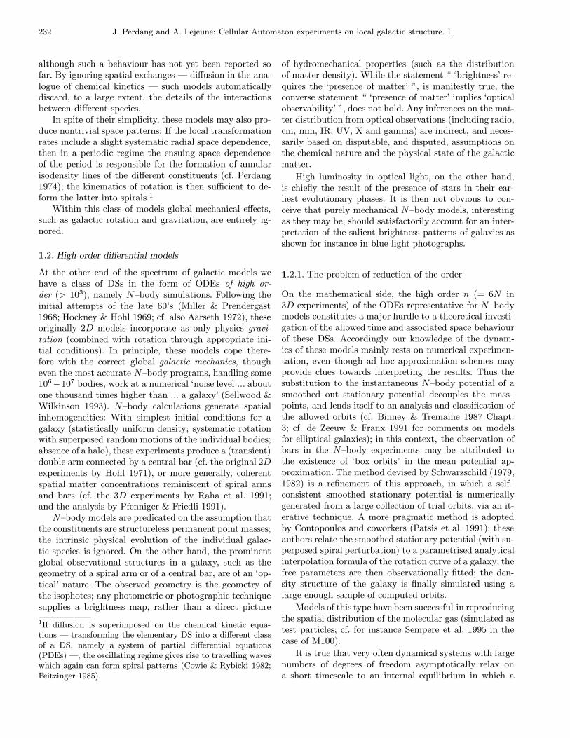
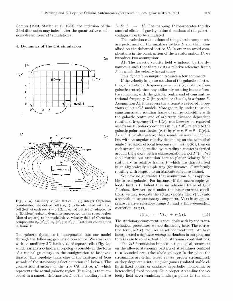
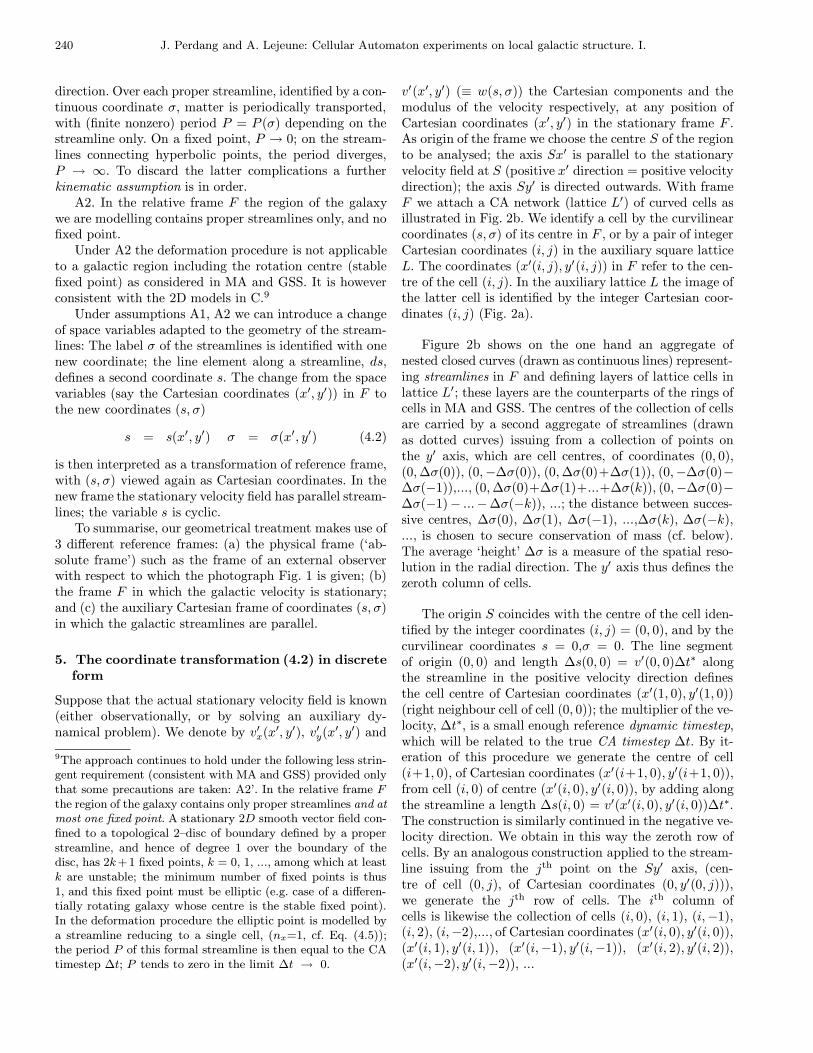
Fig. 2. a) Auxiliary square lattice L; i, j integer Cartesiancoordinates; last dotted cell (right) to be identified with firstcell (left) of each row j = 0,1,2,..., ny. b) Lattice L′ adapted toa (fictitious) galactic dynamics superposed on the space region(dotted square) to be modelled; v, velocity field of Cartesiancomponents vx′(x
′, y′), vy′(x′, y′); x′, y′, Cartesian coordinates
in frame F
The galactic dynamics is incorporated into our modelthrough the following geometric procedure. We start outwith an auxiliary 2D lattice, L, of square cells (Fig. 2a)which assigns a cylindrical topology (possibly in the formof a conical geometry) to the configuration to be inves-tigated; this topology takes care of the existence of localperiods of the stationary galactic motion (cf. below). Thegeometrical structure of the true CA lattice, L′, whichrepresents the actual galactic region (Fig. 2b), is then en-coded in a smooth deformation D of the auxiliary lattice
L, D: L → L′. The mapping D incorporates the dy-namical effects of gravity–induced motions of the galacticconfiguration to be simulated.
The evolution calculations of the galactic componentsare performed on the auxiliary lattice L and then visu-alised on the deformed lattice L′. In order to avoid com-plications in the construction of the transformation D, weintroduce two assumptions.
A1. The galactic velocity field v induced by the dy-namics is such that there exists a relative reference frameF in which the velocity is stationary.
This dynamic assumption requires a few comments.If the velocity is a pure rotation of the galactic substra-
tum, of rotational frequency ω = ω(r) (r, distance fromgalactic centre), then any uniformly rotating frame of cen-tre coinciding with the galactic centre and of constant ro-tational frequency Ω (in particular Ω = 0), is a frame F .Assumption A1 thus covers the alternative studied in pre-vious galactic CA models. More generally, under those cir-cumstances any rotating frame of centre coinciding withthe galactic centre and of arbitrary distance–dependentrotational frequency Ω = Ω(r), can likewise be regardedas a frame F (polar coordinates in F , (r′, θ′), related to thegalactic polar coordinates (r, θ) by r′ = r, θ′ = θ−Ω(r)t).As a further alternative, the streamlines may be circularbut with an angular velocity depending on the azimuthalangle θ (rotation of local frequency ω = w(r)q(θ)); then oneach streamline, identified by its radius r, matter is carriedaround the galaxy with a characteristic period P ∗(r). Weshall restrict our attention here to planar velocity fieldsstationary in relative frames F which are characterisedin an algebraically simple way (for instance, F uniformlyrotating with respect to an absolute reference frame).
We have no guarantee that assumption A1 is applica-ble to real galaxies. For instance, if the macroscopic ve-locity field is turbulent then no reference frame of typeF exists. However, even under the latter extreme condi-tions, we may separate the actual velocity field v(t; r) intoa smooth, mean stationary component, V(r) in an appro-priate relative reference frame F , and a time–dependentcorrection, ν(t; r),
v(t; r) = V(r) + ν(t; r). (4.1)
The stationary component is then dealt with by the trans-formation procedures we are discussing here. The correc-tion term, ν(t; r), requires an ad hoc treatment. We haveincorporated a diffusive mixing mechanism in our programto take care to some extent of nonstationary contributions.
The 2D formulation imposes a topological constrainton the allowed stationary pattern of streamlines confinedto a bounded area (the whole galaxy): In the plane thestreamlines are either closed curves (proper streamlines),or they degenerate into singular points (isolated stable el-liptic fixed points, or unstable hyperbolic [homoclinic orheteroclinic] fixed points). On a proper streamline the ve-locity field never vanishes; it always points in the same
240 J. Perdang and A. Lejeune: Cellular Automaton experiments on local galactic structure. I.
direction. Over each proper streamline, identified by a con-tinuous coordinate σ, matter is periodically transported,with (finite nonzero) period P = P (σ) depending on thestreamline only. On a fixed point, P → 0; on the stream-lines connecting hyperbolic points, the period diverges,P → ∞. To discard the latter complications a furtherkinematic assumption is in order.
A2. In the relative frame F the region of the galaxywe are modelling contains proper streamlines only, and nofixed point.
Under A2 the deformation procedure is not applicableto a galactic region including the rotation centre (stablefixed point) as considered in MA and GSS. It is howeverconsistent with the 2D models in C.9
Under assumptions A1, A2 we can introduce a changeof space variables adapted to the geometry of the stream-lines: The label σ of the streamlines is identified with onenew coordinate; the line element along a streamline, ds,defines a second coordinate s. The change from the spacevariables (say the Cartesian coordinates (x′, y′)) in F tothe new coordinates (s, σ)
s = s(x′, y′) σ = σ(x′, y′) (4.2)
is then interpreted as a transformation of reference frame,with (s, σ) viewed again as Cartesian coordinates. In thenew frame the stationary velocity field has parallel stream-lines; the variable s is cyclic.
To summarise, our geometrical treatment makes use of3 different reference frames: (a) the physical frame (‘ab-solute frame’) such as the frame of an external observerwith respect to which the photograph Fig. 1 is given; (b)the frame F in which the galactic velocity is stationary;and (c) the auxiliary Cartesian frame of coordinates (s, σ)in which the galactic streamlines are parallel.
5. The coordinate transformation (4.2) in discreteform
Suppose that the actual stationary velocity field is known(either observationally, or by solving an auxiliary dy-namical problem). We denote by v′x(x′, y′), v′y(x′, y′) and
9The approach continues to hold under the following less strin-gent requirement (consistent with MA and GSS) provided onlythat some precautions are taken: A2’. In the relative frame Fthe region of the galaxy contains only proper streamlines and atmost one fixed point. A stationary 2D smooth vector field con-fined to a topological 2–disc of boundary defined by a properstreamline, and hence of degree 1 over the boundary of thedisc, has 2k+1 fixed points, k = 0, 1, ..., among which at leastk are unstable; the minimum number of fixed points is thus1, and this fixed point must be elliptic (e.g. case of a differen-tially rotating galaxy whose centre is the stable fixed point).In the deformation procedure the elliptic point is modelled bya streamline reducing to a single cell, (nx=1, cf. Eq. (4.5));the period P of this formal streamline is then equal to the CAtimestep ∆t; P tends to zero in the limit ∆t → 0.
v′(x′, y′) (≡ w(s, σ)) the Cartesian components and themodulus of the velocity respectively, at any position ofCartesian coordinates (x′, y′) in the stationary frame F .As origin of the frame we choose the centre S of the regionto be analysed; the axis Sx′ is parallel to the stationaryvelocity field at S (positive x′ direction = positive velocitydirection); the axis Sy′ is directed outwards. With frameF we attach a CA network (lattice L′) of curved cells asillustrated in Fig. 2b. We identify a cell by the curvilinearcoordinates (s, σ) of its centre in F , or by a pair of integerCartesian coordinates (i, j) in the auxiliary square latticeL. The coordinates (x′(i, j), y′(i, j)) in F refer to the cen-tre of the cell (i, j). In the auxiliary lattice L the image ofthe latter cell is identified by the integer Cartesian coor-dinates (i, j) (Fig. 2a).
Figure 2b shows on the one hand an aggregate ofnested closed curves (drawn as continuous lines) represent-ing streamlines in F and defining layers of lattice cells inlattice L′; these layers are the counterparts of the rings ofcells in MA and GSS. The centres of the collection of cellsare carried by a second aggregate of streamlines (drawnas dotted curves) issuing from a collection of points onthe y′ axis, which are cell centres, of coordinates (0, 0),(0,∆σ(0)), (0,−∆σ(0)), (0,∆σ(0)+∆σ(1)), (0,−∆σ(0)−∆σ(−1)),..., (0,∆σ(0)+∆σ(1)+...+∆σ(k)), (0,−∆σ(0)−∆σ(−1)− ...−∆σ(−k)), ...; the distance between succes-sive centres, ∆σ(0), ∆σ(1), ∆σ(−1), ...,∆σ(k), ∆σ(−k),..., is chosen to secure conservation of mass (cf. below).The average ‘height’ ∆σ is a measure of the spatial reso-lution in the radial direction. The y′ axis thus defines thezeroth column of cells.
The origin S coincides with the centre of the cell iden-tified by the integer coordinates (i, j) = (0, 0), and by thecurvilinear coordinates s = 0,σ = 0. The line segmentof origin (0, 0) and length ∆s(0, 0) = v′(0, 0)∆t∗ alongthe streamline in the positive velocity direction definesthe cell centre of Cartesian coordinates (x′(1, 0), y′(1, 0))(right neighbour cell of cell (0, 0)); the multiplier of the ve-locity, ∆t∗, is a small enough reference dynamic timestep,which will be related to the true CA timestep ∆t. By it-eration of this procedure we generate the centre of cell(i+1, 0), of Cartesian coordinates (x′(i+1, 0), y′(i+1, 0)),from cell (i, 0) of centre (x′(i, 0), y′(i, 0)), by adding alongthe streamline a length ∆s(i, 0) = v′(x′(i, 0), y′(i, 0))∆t∗.The construction is similarly continued in the negative ve-locity direction. We obtain in this way the zeroth row ofcells. By an analogous construction applied to the stream-line issuing from the jth point on the Sy′ axis, (cen-tre of cell (0, j), of Cartesian coordinates (0, y′(0, j))),we generate the jth row of cells. The ith column ofcells is likewise the collection of cells (i, 0), (i, 1), (i,−1),(i, 2), (i,−2),..., of Cartesian coordinates (x′(i, 0), y′(i, 0)),(x′(i, 1), y′(i, 1)), (x′(i,−1), y′(i,−1)), (x′(i, 2), y′(i, 2)),(x′(i,−2), y′(i,−2)), ...
J. Perdang and A. Lejeune: Cellular Automaton experiments on local galactic structure. I. 241
The lines issuing from (0,−∆σ(0)/2), (0, ∆σ(0)/2), (0,−3× ∆σ(0)/2), (0, 3∆σ(0)/2), ..., are again streamlinesspecifying the ‘horizontal’ boundaries of the rows of cells ofthe network L′. The line midway between the centre pointsof columns i − 1 and i represents the common ‘vertical’boundary between the cells of columns i− 1 and i.
This construction provides a cellular network L′
adapted to the stationary velocity field v(r) in frame F .By the same token it defines the correspondence betweenthe lattice L′ and the auxiliary lattice L made up of iden-tical unit square cells (cellsize ∆x = ∆y = 1).
To avoid negative integer coordinates, it is convenientto choose as the origin O of the auxiliary lattice L thelower left corner cell; a cell of L is then specified by (i, j)with i = 0,1,2,...,nx(j) − 1 and j = 0,1,2,...,ny − 1; thenumber of rows (number of cells in the y–direction), ny,is a parameter of the simulation (≈ 103 in our experi-ments); the number of cells per row j, nx(j), depends onthe streamline j (cf. below). Henceforth a point (i, j) in theauxiliary system L will be understood as being defined inthis latter system of nonnegative integer coordinates; thecorresponding cell in the physical lattice L′ (associatedwith the relative frame F ) will be referred to by the samepair (i, j).
The point of Cartesian coordinates (i, j) in L ismapped onto the point of Cartesian coordinates (x′, y′)= (x′(i, j), y′(i, j)) in L′, of the cell of column i and rowj in L′ through the transformation D
D : (i, j) 7→ (x′, y′) = (x′(i, j), y′(i, j)); (5.1)
explicitly, the Cartesian coordinates of the centre pointsof the cells of each row j = 0, 1, ..., ny−1, in L′ are givenby the recurrence relations
x′(i+ 1, j) = x′(i, j) + v′x(x′(i, j), y′(i, j))∆t∗,
y′(i+ 1, j) = y′(i, j) + v′y(x′(i, j), y′(i, j))∆t∗, (5.1a)
(i = 0, 1, ..., nx(j)− 1).10 In the stationary hydrodynamicmotion, the matter content at a position of Cartesian co-ordinates (x′, y′) in the relative frame F is shifted to thenew position
(xN′ , yN′) = (x′ + v′x(x′, y′)∆t∗, y′ + v′y(x′, y′)∆t∗)
in one dynamic timestep ∆t∗, i.e. matter is just translatedto the neighbour cell in the positive velocity direction. De-note by N(Y ; t; x′, y′) and n(Y ; t; x′, y′) the total amountof matter and the corresponding density respectively ofspecies Y at the continuous time t in cell (x′, y′) of L′;
10If a stable fixed point is to be included (assumption A2’),we associate with it a single cell in L′, of ‘height’ ∆σ(0, 0)as above, and ‘width’ ∆s(0, 0) = v′∆t∗; to avoid a flattenedcell we identify v′ with the average cell velocity of the closestproper streamline; this cell is then taken as the origin (0, 0) ofthe coordinate system, with nx(0) = 1. In the auxiliary frameL the ‘lowest’ row then contains a single square cell.
denote further by ∆V (x′, y′) the (time–independent) ‘vol-ume’ of this cell. The discrete CA time, denoted by τ (=0, 1, 2, ...), is related to the continuous time by t = τ∆t,∆t being the automaton timestep; the relation betweenthe kinematic timestep ∆t∗ and the automaton timestep∆t will be discussed below. In the physical lattice L′ theconstraint of conservation of species Y in the mechanicalmotion, over one kinematic timestep ∆t∗, becomes
N(Y ; t; x′, y′) ≡ n(Y ; t; x′, y′)∆V (x′, y′) =
n(Y ; t+ ∆t∗; x′N , y′N)∆V (x′N , y
′N ) ≡
N(Y ; t+ ∆t∗; x′N , y′N). (5.2)
In the auxiliary latticeL, the amount of matter in cell (i, j)is just shifted to cell (i + 1, j) in one kinematic timestep∆t∗, so that the counterpart of (5.2) takes the simple form
N(Y ; t; i, j) = N(Y ; t+ ∆t∗; i+ 1, j). (5.2a)
In this lattice the velocity (= ∆x/∆t∗) is a constant equalto 1 if time is measured in units of the kinematic step ∆t∗.
The comparison of the treatment of a galactic rota-tion by the method initiated in MA with the deformedlattice technique as proposed here, illustrates clearly theadvantage of the latter procedure. Under pure rotation thestreamlines in the physical space are circular (the radius rplaying the role of the coordinate σ); the lattice L′ is madeup of concentric circular rings (labelled by j) subdividedinto cells by roughly radially directed line segments; thesesegments make a progressively smaller angle with the ringsas we go outwards, since the ‘horizontal size’ of the cells,∆s = r∆θ(r) ( ∆θ(r), ‘azimuthal size’), progressively in-creases with increasing distance r from the galactic centre;cells of a ring centred on the same streamline have all samesize. Since in the corresponding auxiliary lattice L matteris shifted by one cell in each row j per timestep ∆t∗, tosecure the correct period P (j) on each proper streamline(row of cells) j, we have to select a number of cells perrow j,nx(j), proportional to P (j) (cf. Eq. (5.3) below).
In the procedures adopted by MA and GSS the cir-cular rings defined by the streamlines are subdivided intocells which all have (approximately) the same width andarea. To incorporate differential rotation, different ringsare rotated by different amounts. If the lattice structurewere preserved in the evolution, as a strict CA frameworkwould require, then in one timestep the jth ring should beshifted by a fixed integer number of cells, hj = 0, 1, 2,...,depending on the label j; two successive rings j, j + 1then would either corotate, (hj+1 − hj = 0), or elsesuffer a relative shift of 1, or 2,... cells per timestep. Incontrast, within the lattice deformation approach we sim-ulate a much slower relative shift of ring j+1 with respectto ring j, namely of 1, 2,... cells per period P (j). Hence a
242 J. Perdang and A. Lejeune: Cellular Automaton experiments on local galactic structure. I.
first advantage of the deformation procedure is that it canrepresent more accurately the differential rotation.11
In the second place, the deformation method is concep-tually closer to the general spirit of CA models: Tradi-tionally CA evolution rules are local rules, predicated oninteractions between neighbour cells only. Unless specialprecautions are taken, the requirement of locality may beviolated in the formal shift procedure, where two neigh-bour cells in adjacent rings may become widely separatedin a single timestep (cf. the experiments in Lejeune & Per-dang 1991 which make use of the shifting method appliedto a local part of the galaxy).
Thirdly, it is not clear how to extend the method ofMA to arbitrary stationary motions.12
A closed streamline j in the galaxy is simulated by thecomplete ring j of cells of the physical lattice L′,nx(j) be-ing then the total number of cells in this ring. In contrastto the method of MA which models the whole galaxy, ourpurpose is to devise a procedure describing the behaviourof a small part of the galaxy only (rectangular zone Rin Fig. 2b), thereby avoiding an explicit treatment of therest of the galaxy. Accordingly, we do not attempt to de-scribe the whole ring but only a small section of it. Tothis end we embed R in a larger region Z (covered by thefinite network L′); Z remains small as compared to thewhole galaxy. The number of cells nx(j) thus representsthe number of cells of ring j within the region Z in whichwe carry out our computations. The behaviour of the re-mainder of the galaxy is not explicitly treated; its effect isdealt with through boundary conditions at the border ofzone Z.
In the case of a closed streamline j in the relative frameF (lattice L′), the kinematic timestep ∆t∗ and the periodP (j) associated with this streamline, determine the totalnumber of cells, nx(j), in the full ring j defined by thisstreamline, namely nx(j) ≈ P (j)/∆t∗. In a rigorous
11In practice, the accuracy in the ring shifting method isimproved by actually shifting successive rings by fractionalamounts of the cell size; however, such a procedure does notconform to a standard CA methodology.12In the deformation method the stationarity assumption A1 ofthe velocity field in the 2D galactic model, and the kinematicassumption A2 (or A2’) appear as essential ingredients. Onlyunder these assumptions do we secure a simple geometry of thestreamlines, and hence the existence of a geometrically simpleauxiliary lattice L. In the presence of several fixed points (vi-olation of A2’) the elementary structure of an auxiliary latticeL is not only destroyed: it also raises the problem of handlingstreamlines connecting unstable fixed points. We should finallystress the special constraint imposed by the dimensionality 2of our simulation. In a 3D space stationarity of a velocity fieldconfined to a bounded region does not automatically imply pe-riodicity; stationary streamlines in 3D confined to a boundedregion may not close, in which case they either correspond tomulti–periodic, or else to chaotic transport of matter. It is notclear how the latter alternative could be simulated kinemati-cally in a CA environment.
treatment the full ring should be dealt with; in the latter,cell i = 0 is identical with cell i = nx(j), a property whichcan be interpreted as a boundary condition. In our localformulation nx(j) represents a fraction f ≈ 1/K (K, aninteger independent of j if the region Z is properly chosen)of the total number of cells of the closed streamline j. Thenumber of cells in the section of the streamline lying in Zis thus given by
nx(j) ≈ P (j)
K∆t∗. (5.3)
This procedure is consistent with the true period for thetransport of matter on the streamline j. In the present casean explicit boundary condition is needed; to this end, justas for the full ring, we identify cells i = 0 and nx(j) oneach streamline j (cf. the auxiliary lattice Fig. 2a wherethe dotted cell on the right is identified with the first cellon the left).13
The boundary conditions we are then led to adopt are
state of cell (nx(j), j) ≡ state of cell (0, j),
state of cell (−1, j) ≡ state of cell (nx(j) − 1, j).(5.4)
The latter condition is needed when dealing with theneighbourhood of cell (0, j).14
At the bottom (j = 0) and top rows (j = ny − 1) weimpose artificial reflection conditions. The ‘lower’ neigh-bour of a cell in the bottom row, (i, 0), is identified with its‘upper’ neighbour; and the ‘upper’ neighbour of a cell ofthe top row, (i, nx) is identified with the ‘lower’ neighbourof this cell
state of cell (i,−1) ≡ state of cell (i,+1),
state of cell (i, ny) ≡ state of cell (i, ny−2). (5.5)
For an endcell (nx(j) − 1, j) of a row, the ‘lower’ and‘upper’ neighbours are read off from Fig. 2a. The latterconditions are required for the specification of the neigh-bourhood of a boundary cell.15
13Geometrically this imposes a fictitious K–fold symmetry tothe global structure of the galaxy; but since the modelling pro-cedure only deals with 1/K of the ring, this symmetry neverbecomes observable in the simulation. With K integer, the trueperiodicity P (j) remains an exact period of the motion alongthe streamline.14The approach we have adopted is reminiscent of a methodapplied in statistical mechanics: instead of computing for in-stance the behaviour of a gas in a large vessel, the gas is for-mally confined to a small cubic test region, and simple peri-odicity conditions are imposed on the surface of the cube; theidea is that the precise form of the boundary conditions doesnot influence significantly the behaviour inside the test cube.15We should keep in mind that since neighbour rows have gen-erally different numbers of cells nx(j), after a time intervalP (j)/K row j is shifted with respect to its neighbour rows.Matter initially in say column 0 thus distributes over several
J. Perdang and A. Lejeune: Cellular Automaton experiments on local galactic structure. I. 243
6. CA simulation of star formation and stellarevolution
As in our previous simulations (Perdang 1990; Lejeune &Perdang 1991; Lejeune 1993), the following galactic speciesare dealt with in the evolutionary computations: interstel-lar gas and dust, D, (in the form of molecular clouds);massive protostars, P ; massive main sequence stars, M ,massive evolved stars (referred to as ‘red giants’) R; in-ert remnants (white dwarfs, neutron stars, black holes), I;and low mass stars, L. A given cell (i, j) in lattice L′ orin the auxiliary lattice L, is either empty, E, or populatedby at most one of the 6 species listed. The field functionF (τ ; i, j) encoding the state of cell (i, j) at discrete timeτ , is defined over ZZ7; (7–state automaton; F = 0: emptystate E, black in our colour plates; F = 1: gas state D,cyan; F = 2: P , white; F = 3: M , yellow; F = 4: R, red;F = 5: I blue; and F = 6: L magenta).
There is manifestly considerable freedom in the defini-tion of ‘massive’ and ‘low mass’ stellar objects. We havehere in mind representative orders of magnitude for the P ,M and R objects of 15−20 M; L objects are assignedmasses of about 1 M or lower. The choice of a mass range> 15 M for massive stars is dictated by the requirementthat the surface brightness of the galaxy be dominated bythe luminosity of these objects (in their early evolutionaryphase P ; luminosity> 105 L for >15 M). On the otherhand, with the assignment of a mass of 1 M to species L,low mass stars do not significantly evolve over the times-pan of an experimental run (not substantially exceeding108 y); for the purposes of evolution both states L and Ithen play the parts of sinks for the galactic material. Overthe same timespan of one run a massive star goes througha full evolutionary cycle; at the end of the cycle most ofthe star’s matter is returned into the active gas form D;a new cycle then starts all over again.
If we adopt a surface density of matter of the order ofthe solar neighbourhood density, (≈ 75 M/pc2; Binney& Tremaine 1987), then a cell of our 103×103 automaton(simulating a total area of 16 kpc2), if not empty, carriesan average mass of roughly 103 M; the cell has a size ofthe order of the size of a cluster or an association. If in aP , M or R state, then the cell contains approximately 50actual protostars, main sequence stars or red giants; if inan L or I state, it contains 103 low mass or inert stars.
columns after a time > P/K , where P is the period associatedwith any streamline. Under the amended assumption A2’, inthe presence of a stable fixed point the right and left neigh-bours of the corresponding cell (0, 0) are to be identified withthe cell (0, 0) itself, in conformity with Eq. (5.4); the shift ofmatter to the neighbour cell in one timestep thus leaves thiscell unchanged. The region in physical space containing thefixed point surrounds the latter; in the simulation on latticeL′ cell (0,0) is thus surrounded by a ring of 8 cells, with thefirst and last cells of the ring being physical neighbours; theperiodicity condition (5.4) is then exact.
With our evolution processes being handled on the levelof cellstates rather than on the level of actual galactic ob-jects, the physical parameters referring to stars (transitionprobabilities per timestep) must be rescaled to individualcells.16
The stellar evolutionary processes accounted for in ourmodel are transformations among the 6 galactic species,simulated by transitions among the 6 non–empty cellstatesof our CA model. These transformations are convenientlyvisualised as chemical reactions symbolised by stoichio-metric schemes of the form
X + nC + mK + ... →
Y + nC + mK + ..., P [X, nC,mK, ...; Y, nC,mK, ...].(6.1)
This notation means that if at discrete time τ cell (i, j)is in state X, and n cells (i′, j′), (i′′, j′′),..., of the neigh-bourhood IN(i, j) of cell (i, j) are in state C, m cells ofthe neighbourhood are in state K, etc, then at discretetime τ + 1 state X is replaced by state Y with probabil-ity P [X, nC,mK, ...;Y, nC,mK, ...]. The neighbourhoodIN(i, j) we adopt is the Moore neighbourhood, consistingof the cell (i, j) itself and its 8 neighbours (i, j±1), (i±1, j)and (i±1, j±1). Species C, K, ... act as catalysts. In thissection we regard times are being expressed in units of anevolutionary timestep, ∆t∗∗, adapted to the evolutionarytimescale of our massive objects, ∆t∗∗ ≈ 5 105 y.
The initial state of the galaxy is a diffuse and spatiallynon–uniform aggregate of gas: any cellstate F (0; i, j) iseither 0 (E state), or 1 (D state) (cf. Paper II).
6.1. Star formation
The two protostar formation processes already imple-mented in the model of MA as well as in all subsequentCA models are naturally included in our formulation:
(α) Spontaneous gravitational collapse of interstellarmatter (molecular clouds) into protostars, as a result of aJeans instability.
We regard the latter as being operative at a given sitein the galaxy provided that a large enough neighbourhoodcontains interstellar matter; essentially the latter provisoguarantees that a critical wavelength may actually be re-alised in the neighbourhood of the site. Spontaneous starformation produces both low mass stars and massive stars.The corresponding stoichiometric schemes are
D + dD → P + dD; P [DdD;PdD] (6.2)
D + eD → L + eD; P [DeD;LeD] (6.3)
we have set d ≥ 5 and e ≥ 2. The probabilities of theseprocesses are chosen small enough, 5 10−5 (P –formation)
16With 103 P cells in a 103×103 automaton (about 0.1% of thematter in P form) the average luminosity/pc2 for a region of4×4 kpc2 is ≈ 300 L/pc2 (order of central surface brightnessof elliptical galaxies: 140 L/pc2; Binney & Tremaine 1987).
244 J. Perdang and A. Lejeune: Cellular Automaton experiments on local galactic structure. I.
and 1.7 10−4 (L–formation) per timestep ∆t∗∗; the pre-cise value of the P –formation rate by process (6.2) is foundto be immaterial for the actual evolution of the galacticmatter; this process is indeed obliterated by star–inducedstar formation (β), as soon as a few protostars are presentin the medium; the role of a small transition probabilityof (6.2) is to delay the efficient onset of star formationthrough the explosive catalytic process (β) discussed be-low. Test experiments, with an initial state inseminatedby just a few protostars (≈ 10 in a lattice of 106 cells) andwith process (6.2) entirely suppressed, demonstrate thatthe subsequent evolution of the galactic species is virtuallyidentical with the original evolution.
(β) Catalytic protostar formation. The global stoichio-metric scheme symbolising this process is
D + pP + mM + rR →
P + pP + mM + rR; P [DpPmMrR;PpPmMrR],(6.4)
which is our counterpart of the more schematic process(1.2) of MA. Since catalytic star enhanced star formationconstitutes the main ingredient of SPSF, advocated in allCA simulations of galactic structure (cf. GSS), it is su-perfluous to rehash the arguments in favour of this mech-anism. In our numerical implementation we require thatp+ r ≥ 1, or m ≥ 4, expressing that luminous young ob-jects or luminous evolved stars (which end as supernovae)have a far more efficient triggering action than massivemain sequence stars (a Moore neighbourhood with at least4 M cells having a virtually vanishing probability to ma-terialise).
The numerical values we have adopted for the transi-tion probability of process (6.4) lie in the range 0.03−0.3per timestep ∆t∗∗. In GSS this probability is the mainmodel parameter responsible for the onset of the percola-tion phase transition.
6.2. Stellar evolution
Besides the usual evolutionary steps of isolated stars
P → M ; P [P ;M ], (6.5)
M → R; P [M ;R], (6.6)
R → I; P [R; I], (6.7)
L → I; P [L; I], (6.8)
whose transition probabilities are provided by standardstellar evolution, we add artificial steps of disintegrationfor each ‘active’ stellar species A into gas
A → D; A = P,M,R or L; P [A;D]; (6.9)
the latter simulate mass loss accompanying the normalevolution of all massive stars, as well as the cataclysmiclate evolutionary stages.
The orders of magnitude of the transition probabilitiesper timestep we adopt are P [P ;M ] ≈ 0.002; P [M ;R] ≈0.02; P [R; I] ≈ 5 10−4; P [L; I] ≈ 4 10−6; with the latter‘disintegration’ probability of the L objects this mecha-nism is inoperative over the timescale of our experiments.The estimate of the transition probabilities is illustratedin the case of P [R; I]: A genuine massive red giant trans-forms about 1/15th to 1/20th of its matter into inert ob-jects, the remainder being recycled as gas; if we take atimescale of 5 107 y for the massive red giant phase, since15 to 20 R cells are needed to form one I cell, the effectivetimescale for the formation of one I cell becomes ≈ 109 y;hence we have a probability per timestep of the order of∆t∗∗/109 ≈ 5 10−4.
As tentative orders for the probabilities of mass losswe adopt P [P ;D] ≈ 0.09; P [M ;D] ≈ 0.025; P [R;D] ≈0.1; P [L;D] < 0.0001.
In addition to the standard stellar evolutionary steps(6.5-8) we include catalytic steps which are meant to re-flect the property that in a close multiple stellar systemthe evolution of an individual component is affected by itscompanions (essentially through exchange of mass). Weinclude the following schemes
P + pP + mM + rR →
M + pP + mM + rR; P [PpPmMrR;MpPmMrR],(6.10)
M + rR → R + rR; P [MrR;RrR]. (6.11)
The first reaction mechanism, which we let operate ifp + r ≥ 1 or m ≥ 4 (cf. above), captures the transfor-mation of a protostar into a main sequence star under theeffect of the extra radiation field of the companions; wehave here tentatively set this probability equal to 0.05.The second process (with r ≥ 1) symbolises the evolu-tion of a main sequence star in a close binary or in ahigher order multiple stellar system. The transformationrate of the main sequence star into a red giant in the pres-ence of one or several more evolved companions is speededup, as a result of mass transfer from the evolved (R) tothe less evolved body (M). In our test experiments wehave typically chosen P [MrR;RrR] ≈ 0.075. Physicallythe evolution of a main sequence star in a close binary isnot a genuine catalytic step, since both components, themain sequence star and the red giant undergo mutuallyinduced evolutionary changes. By formally approximatingthis evolutionary stage by (6.11) we disregard the fact thatwhile suffering mass loss, the R cell suffers a change in itsevolutionary rate as well; the reaction step (6.11) only du-plicates the effect of mass accretion on the M cell whoseevolution thereby may be affected significantly.
It was noticed in the context of simplest ODE models(1) that the combined presence of the catalytic steps (6.4)and (6.11) in the network of evolutionary transformationscan lead to oscillations in the global average of the popula-tion of the different species (Perdang 1974). The numerical
J. Perdang and A. Lejeune: Cellular Automaton experiments on local galactic structure. I. 245
experiments carried out with the present CA model notonly confirm the possibility of a periodic time behaviourin the spatially extended system, for specific choices of theparameters; they also indicate that a transition to spatialinhomogeneity can take place, reminiscent of the spatialsymmetry breaking in reaction–diffusion systems and in-duced by an instability in the reaction scheme (Prigogine& Lefever 1968; Glansdorff & Prigogine 1971). In chem-ical reactions one necessary condition for any symmetrybreaking, temporal or spatial, is the presence of catalyticsteps in the stoichiometric equations; a second quantita-tive condition is that the timescales in the different reac-tion steps inducing the instability be of same order. Underusual conditions prevailing in a galaxy, the latter require-ment is probably not fulfilled, so that this dynamic regimeseems to be of marginal astrophysical interest only.
6.3. Other effects
The model includes an inflow of gas from the galactic haloonto the disk during the early galactic evolution. This issimulated by a gas ‘creation’ scheme
E → D, P [E;D]; (6.12)
The corresponding transition probability is set equal to1 10−5, during the first 100 evolutionary timesteps (con-traction phase of galaxy); it drops to zero at later times.
As an admittedly rough way of accounting for propermotions, as well as for non–stationary irregular hydrody-namics, we implement a spatial diffusion or mixing mech-anism affecting all of the galactic species in the same way.As in our previous papers, this is done via the simplealgorithm of Chopard & Droz (1990). The random quasi–isotropic mixing is applied in the auxiliary lattice L, sothat in the physical frame L′ isotropy of the irregular mo-tions appears as broken, as it should do.
For the simplest evolution processes of isolated stars(6.5-6.8), stellar evolution theory supplies, in principle, re-liable timescales for individual masses. The relevant tran-sition probabilities for our model are averaged inversetimescales over the stellar mass distribution. Our artifi-cial subdivision of the stellar mass spectrum into just twocategories, low mass stars and massive stars, makes theseprobabilities strongly dependent on the specific mass atwhich the subdivision occurs; moreover these probabilitiesdepend on the precise form of the mass spectrum and es-pecially on cut–offs. This leaves considerable uncertaintyeven in these transition probabilities. The characteristictimes for star formation, for the processes of mass loss, andfor the catalytic steps (6.10, 11), can only be guessed at;the ‘reaction rates’ for these processes must be regardedas free parameters. The main goal of the present work isto show that physical and geometrical observational in-formation (relative amounts of different galactic species,local fractal dimension of arms, etc, in real galaxies) maybe used to constrain these parameters.
7. Stationary velocity field of the CA model
The velocity pattern we select (over a square area R ofabout 16 kpc2, of centre at a distance rS = 6 kpc fromthe galactic centre) is required to possess characteristicproperties generic for actual galactic fields. Therefore wechoose a velocity field which is rotational on average, ofthe order of 200 km s−1, and which increases outwardsby several km s−1 per kpc. In an absolute reference frameour ansatz for the angle–averaged azimuthal velocity at adistance r from the galactic centre O is
vo(r) = va + (r − rS)v′b,
va ≈ 200 kms−1, v′b ≈ 3.5 kms−1/kpc. (7.1)
We assume that the complete velocity field differs fromthe average field by correction factors less than 10% ofthe value of va.17
In conformity with assumptions A1, A2 we postulatethe existence of a relative reference frame F in which thetrue velocity field is stationary and has no fixed points. Weapproximate this reference system by a frame in uniformrotation with respect to the absolute frame; the order ofmagnitude of the period PF of frame F with respect tothe absolute frame will be chosen close enough to P (S);within F the angle–averaged velocity then becomes
vo∗(r) = v∗a + (r − rS)v′b, va
∗ va, in F ; (7.1a)
(without loss we require vo∗(r) > 0 in the region to be
modelled). The absence of fixed points is secured if wehave
v∗a > (rS − rmin)v′b or va∗ > 7 km/s (7.1b)
for the orders of magnitude adopted.We describe the full (non–averaged) stationary velocity
field in zone Z embedding R in polar coordinates, by aFourier–type ansatz of the form
Vθ(r, θ) = vo∗(r) +
v1(r) sin(2πθ/Θ(r)+Φ1(r)) + v2(r) sin(4πθ/Θ(r)+Φ2(r)),
VR(r, θ) = w1(r) sin(2πθ/Θ(r) + φ1(r))+
w2(r) sin(4πθ/Θ(r) + φ2(r)). (7.2)
17These orders of magnitude are consistent with the rotationvelocity in our Galaxy (va = 220 km s−1 for solar neighbour-hood, distance ≈ 8.5 kpc; A–value of galactic rotation curve:13.3 ±1.5 km s−1/kpc, Hron & Maitzen 1985; we have chosenhere a somewhat smaller gradient). With the average rotationalvelocity it takes 2 107 y for matter on the streamline passingthrough the centre S to be shifted from one side to the otherin our model. This corresponds to 1/10th of the local periodP (S) (rotation period of solar neighbourhood: 2.4 108 y).
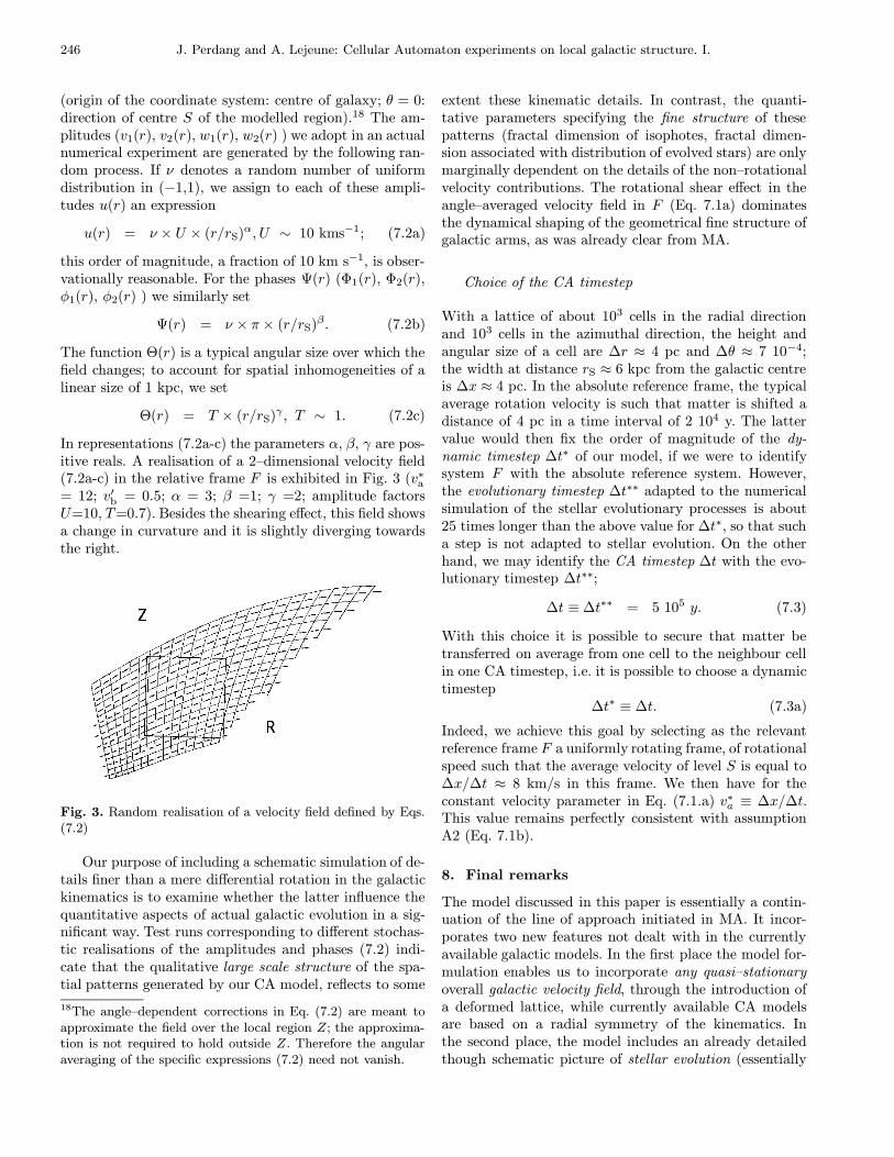
246 J. Perdang and A. Lejeune: Cellular Automaton experiments on local galactic structure. I.
(origin of the coordinate system: centre of galaxy; θ = 0:direction of centre S of the modelled region).18 The am-plitudes (v1(r), v2(r), w1(r), w2(r) ) we adopt in an actualnumerical experiment are generated by the following ran-dom process. If ν denotes a random number of uniformdistribution in (−1,1), we assign to each of these ampli-tudes u(r) an expression
u(r) = ν × U × (r/rS)α, U ∼ 10 kms−1; (7.2a)
this order of magnitude, a fraction of 10 km s−1, is obser-vationally reasonable. For the phases Ψ(r) (Φ1(r), Φ2(r),φ1(r), φ2(r) ) we similarly set
Ψ(r) = ν × π × (r/rS)β. (7.2b)
The function Θ(r) is a typical angular size over which thefield changes; to account for spatial inhomogeneities of alinear size of 1 kpc, we set
Θ(r) = T × (r/rS)γ , T ∼ 1. (7.2c)
In representations (7.2a-c) the parameters α, β, γ are pos-itive reals. A realisation of a 2–dimensional velocity field(7.2a-c) in the relative frame F is exhibited in Fig. 3 (v∗a= 12; v′b = 0.5; α = 3; β =1; γ =2; amplitude factorsU=10, T=0.7). Besides the shearing effect, this field showsa change in curvature and it is slightly diverging towardsthe right.
Fig. 3. Random realisation of a velocity field defined by Eqs.(7.2)
Our purpose of including a schematic simulation of de-tails finer than a mere differential rotation in the galactickinematics is to examine whether the latter influence thequantitative aspects of actual galactic evolution in a sig-nificant way. Test runs corresponding to different stochas-tic realisations of the amplitudes and phases (7.2) indi-cate that the qualitative large scale structure of the spa-tial patterns generated by our CA model, reflects to some
18The angle–dependent corrections in Eq. (7.2) are meant toapproximate the field over the local region Z; the approxima-tion is not required to hold outside Z. Therefore the angularaveraging of the specific expressions (7.2) need not vanish.
extent these kinematic details. In contrast, the quanti-tative parameters specifying the fine structure of thesepatterns (fractal dimension of isophotes, fractal dimen-sion associated with distribution of evolved stars) are onlymarginally dependent on the details of the non–rotationalvelocity contributions. The rotational shear effect in theangle–averaged velocity field in F (Eq. 7.1a) dominatesthe dynamical shaping of the geometrical fine structure ofgalactic arms, as was already clear from MA.
Choice of the CA timestep
With a lattice of about 103 cells in the radial directionand 103 cells in the azimuthal direction, the height andangular size of a cell are ∆r ≈ 4 pc and ∆θ ≈ 7 10−4;the width at distance rS ≈ 6 kpc from the galactic centreis ∆x ≈ 4 pc. In the absolute reference frame, the typicalaverage rotation velocity is such that matter is shifted adistance of 4 pc in a time interval of 2 104 y. The lattervalue would then fix the order of magnitude of the dy-namic timestep ∆t∗ of our model, if we were to identifysystem F with the absolute reference system. However,the evolutionary timestep ∆t∗∗ adapted to the numericalsimulation of the stellar evolutionary processes is about25 times longer than the above value for ∆t∗, so that sucha step is not adapted to stellar evolution. On the otherhand, we may identify the CA timestep ∆t with the evo-lutionary timestep ∆t∗∗;
∆t ≡ ∆t∗∗ = 5 105 y. (7.3)
With this choice it is possible to secure that matter betransferred on average from one cell to the neighbour cellin one CA timestep, i.e. it is possible to choose a dynamictimestep
∆t∗ ≡ ∆t. (7.3a)
Indeed, we achieve this goal by selecting as the relevantreference frame F a uniformly rotating frame, of rotationalspeed such that the average velocity of level S is equal to∆x/∆t ≈ 8 km/s in this frame. We then have for theconstant velocity parameter in Eq. (7.1.a) v∗a ≡ ∆x/∆t.This value remains perfectly consistent with assumptionA2 (Eq. 7.1b).
8. Final remarks
The model discussed in this paper is essentially a contin-uation of the line of approach initiated in MA. It incor-porates two new features not dealt with in the currentlyavailable galactic models. In the first place the model for-mulation enables us to incorporate any quasi–stationaryoverall galactic velocity field, through the introduction ofa deformed lattice, while currently available CA modelsare based on a radial symmetry of the kinematics. Inthe second place, the model includes an already detailedthough schematic picture of stellar evolution (essentially
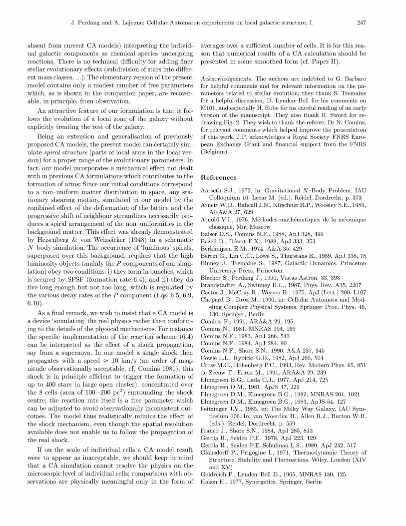
J. Perdang and A. Lejeune: Cellular Automaton experiments on local galactic structure. I. 247
absent from current CA models) interpreting the individ-ual galactic components as chemical species undergoingreactions. There is no technical difficulty for adding finerstellar evolutionary effects (subdivision of stars into differ-ent mass classes, ...). The elementary version of the presentmodel contains only a modest number of free parameterswhich, as is shown in the companion paper, are recover-able, in principle, from observation.
An attractive feature of our formulation is that it fol-lows the evolution of a local zone of the galaxy withoutexplicitly treating the rest of the galaxy.
Being an extension and generalisation of previouslyproposed CA models, the present model can certainly sim-ulate spiral structure (parts of local arms in the local ver-sion) for a proper range of the evolutionary parameters. Infact, our model incorporates a mechanical effect not dealtwith in previous CA formulations which contributes to theformation of arms: Since our initial conditions correspondto a non–uniform matter distribution in space, any sta-tionary shearing motion, simulated in our model by thecombined effect of the deformation of the lattice and theprogressive shift of neighbour streamlines necessarily pro-duces a spiral arrangement of the non–uniformities in thebackground matter. This effect was already demonstratedby Heisenberg & von Weizsacker (1948) in a schematicN–body simulation. The occurrence of ‘luminous’ spirals,superposed over this background, requires that the highluminosity objects (mainly the P components of our simu-lation) obey two conditions: i) they form in bunches, whichis secured by SPSF (formation rate 6.4); and ii) they dolive long enough but not too long, which is regulated bythe various decay rates of the P component (Eqs. 6.5, 6.9,6.10).
As a final remark, we wish to insist that a CA model isa device ‘simulating’ the real physics rather than conform-ing to the details of the physical mechanisms. For instancethe specific implementation of the reaction scheme (6.4)can be interpreted as the effect of a shock propagation,say from a supernova. In our model a single shock thenpropagates with a speed ≈ 10 km/s (an order of mag-nitude observationally acceptable, cf. Comins 1981); thisshock is in principle efficient to trigger the formation ofup to 400 stars (a large open cluster), concentrated overthe 8 cells (area of 100−200 pc2) surrounding the shockcentre; the reaction rate itself is a free parameter whichcan be adjusted to avoid observationally inconsistent out-comes. The model thus realistically mimics the effect ofthe shock mechanism, even though the spatial resolutionavailable does not enable us to follow the propagation ofthe real shock.
If on the scale of individual cells a CA model resultwere to appear as inacceptable, we should keep in mindthat a CA simulation cannot resolve the physics on themicroscopic level of individual cells; comparisons with ob-servations are physically meaningful only in the form of
averages over a sufficient number of cells. It is for this rea-son that numerical results of a CA calculation should bepresented in some smoothed form (cf. Paper II).
Acknowledgements. The authors are indebted to G. Barbarofor helpful comments and for relevant information on the pa-rameters related to stellar evolution; they thank S. Tremainefor a helpful discussion, D. Lynden–Bell for his comments onM101, and especially H. Robe for his careful reading of an earlyversion of the manuscript. They also thank R. Sword for re-drawing Fig. 2. They wish to thank the referee, Dr N. Comins,for relevant comments which helped improve the presentationof this work. J.P. acknowledges a Royal Society–FNRS Euro-pean Exchange Grant and financial support from the FNRS(Belgium).
References
Aarseth S.J., 1972, in: Gravitational N–Body Problem, IAUColloquium 10. Lecar M. (ed.). Reidel, Dordrecht, p. 373
Arnett W.D., Bahcall J.N., Kirschner R.P., Woosley S.E., 1989,ARA&A 27, 629
Arnold V.I., 1976, Methodes mathematiques de la mecaniqueclassique, Mir, Moscow
Balser D.S., Comins N.F., 1988, ApJ 328, 499Bazell D., Desert F.X., 1988, ApJ 333, 353Berkhuijsen E.M., 1974, A&A 35, 429Bertin G., Lin C.C., Lowe S., Thurstans R., 1989, ApJ 338, 78Binney J., Tremaine S., 1987, Galactic Dynamics. Princeton
University Press, PrincetonBlacher S., Perdang J., 1990, Vistas Astron. 33, 393Brandstadter A., Swinney H.L., 1987, Phys. Rev. A35, 2207Castor J., McCray R., Weaver R., 1975, ApJ (Lett.) 200, L107Chopard B., Droz M., 1990, in: Cellular Automata and Mod-
eling Complex Physical Systems, Springer Proc. Phys. 46,130. Springer, Berlin
Combes F., 1991, ARA&A 29, 195Comins N., 1981, MNRAS 194, 169Comins N.F., 1983, ApJ 266, 543Comins N.F., 1984, ApJ 284, 90Comins N.F., Shore S.N., 1990, A&A 237, 345Cowie L.L., Rybicki G.B., 1982, ApJ 260, 504Cross M.C., Hohenberg P.C., 1993, Rev. Modern Phys. 65, 851de Zeeuw T., Franx M., 1991, ARA&A 29, 239Elmegreen B.G., Lada C.J., 1977, ApJ 214, 725Elmegreen D.M., 1981, ApJS 47, 229Elmegreen D.M., Elmegreen B.G., 1982, MNRAS 201, 1021Elmegreen D.M., Elmegreen B.G., 1983, ApJS 54, 127Feitzinger J.V., 1985, in: The Milky Way Galaxy, IAU Sym-
posium 106. In: van Woerden H., Allen R.J., Burton W.B.(eds.). Reidel, Dordrecht, p. 559
Franco J., Shore S.N., 1984, ApJ 285, 813Gerola H., Seiden P.E., 1978, ApJ 223, 129Gerola H., Seiden P.E.,Schulman L.S., 1980, ApJ 242, 517Glansdorff P., Prigogine I., 1971, Thermodynamic Theory of
Structure, Stability and Fluctuations. Wiley, London (XIVand XV)
Goldreich P., Lynden–Bell D., 1965, MNRAS 130, 125Haken H., 1977, Synergetics. Springer, Berlin
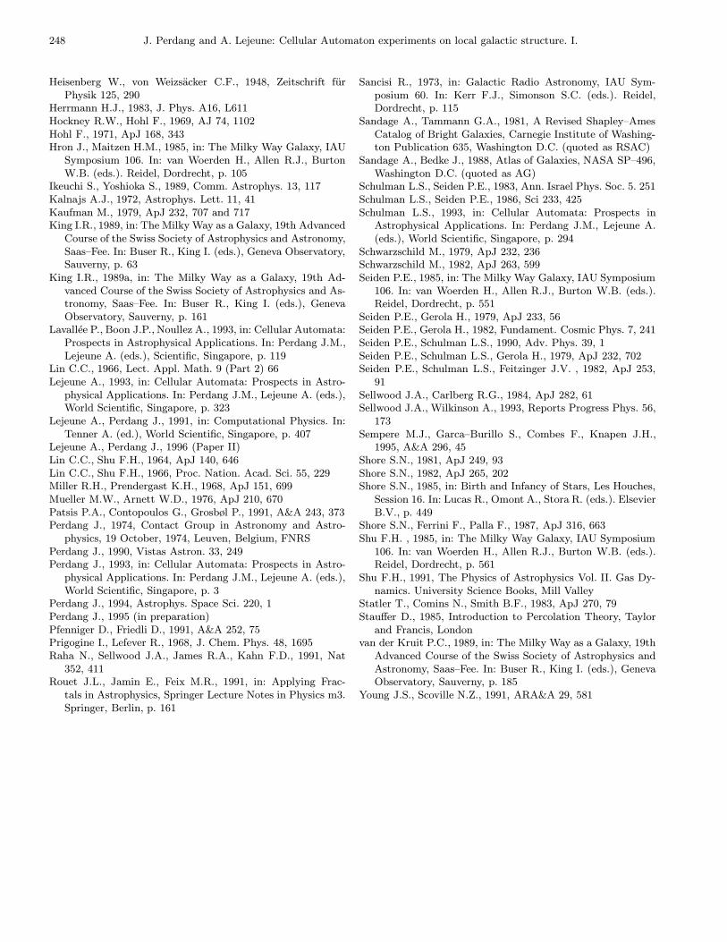
248 J. Perdang and A. Lejeune: Cellular Automaton experiments on local galactic structure. I.
Heisenberg W., von Weizsacker C.F., 1948, Zeitschrift furPhysik 125, 290
Herrmann H.J., 1983, J. Phys. A16, L611Hockney R.W., Hohl F., 1969, AJ 74, 1102Hohl F., 1971, ApJ 168, 343Hron J., Maitzen H.M., 1985, in: The Milky Way Galaxy, IAU
Symposium 106. In: van Woerden H., Allen R.J., BurtonW.B. (eds.). Reidel, Dordrecht, p. 105
Ikeuchi S., Yoshioka S., 1989, Comm. Astrophys. 13, 117Kalnajs A.J., 1972, Astrophys. Lett. 11, 41Kaufman M., 1979, ApJ 232, 707 and 717King I.R., 1989, in: The Milky Way as a Galaxy, 19th Advanced
Course of the Swiss Society of Astrophysics and Astronomy,Saas–Fee. In: Buser R., King I. (eds.), Geneva Observatory,Sauverny, p. 63
King I.R., 1989a, in: The Milky Way as a Galaxy, 19th Ad-vanced Course of the Swiss Society of Astrophysics and As-tronomy, Saas–Fee. In: Buser R., King I. (eds.), GenevaObservatory, Sauverny, p. 161
Lavallee P., Boon J.P., Noullez A., 1993, in: Cellular Automata:Prospects in Astrophysical Applications. In: Perdang J.M.,Lejeune A. (eds.), Scientific, Singapore, p. 119
Lin C.C., 1966, Lect. Appl. Math. 9 (Part 2) 66Lejeune A., 1993, in: Cellular Automata: Prospects in Astro-
physical Applications. In: Perdang J.M., Lejeune A. (eds.),World Scientific, Singapore, p. 323
Lejeune A., Perdang J., 1991, in: Computational Physics. In:Tenner A. (ed.), World Scientific, Singapore, p. 407
Lejeune A., Perdang J., 1996 (Paper II)Lin C.C., Shu F.H., 1964, ApJ 140, 646Lin C.C., Shu F.H., 1966, Proc. Nation. Acad. Sci. 55, 229Miller R.H., Prendergast K.H., 1968, ApJ 151, 699Mueller M.W., Arnett W.D., 1976, ApJ 210, 670Patsis P.A., Contopoulos G., Grosbøl P., 1991, A&A 243, 373Perdang J., 1974, Contact Group in Astronomy and Astro-
physics, 19 October, 1974, Leuven, Belgium, FNRSPerdang J., 1990, Vistas Astron. 33, 249Perdang J., 1993, in: Cellular Automata: Prospects in Astro-
physical Applications. In: Perdang J.M., Lejeune A. (eds.),World Scientific, Singapore, p. 3
Perdang J., 1994, Astrophys. Space Sci. 220, 1Perdang J., 1995 (in preparation)Pfenniger D., Friedli D., 1991, A&A 252, 75Prigogine I., Lefever R., 1968, J. Chem. Phys. 48, 1695Raha N., Sellwood J.A., James R.A., Kahn F.D., 1991, Nat
352, 411Rouet J.L., Jamin E., Feix M.R., 1991, in: Applying Frac-
tals in Astrophysics, Springer Lecture Notes in Physics m3.Springer, Berlin, p. 161
Sancisi R., 1973, in: Galactic Radio Astronomy, IAU Sym-posium 60. In: Kerr F.J., Simonson S.C. (eds.). Reidel,Dordrecht, p. 115
Sandage A., Tammann G.A., 1981, A Revised Shapley–AmesCatalog of Bright Galaxies, Carnegie Institute of Washing-ton Publication 635, Washington D.C. (quoted as RSAC)
Sandage A., Bedke J., 1988, Atlas of Galaxies, NASA SP–496,Washington D.C. (quoted as AG)
Schulman L.S., Seiden P.E., 1983, Ann. Israel Phys. Soc. 5. 251Schulman L.S., Seiden P.E., 1986, Sci 233, 425Schulman L.S., 1993, in: Cellular Automata: Prospects in
Astrophysical Applications. In: Perdang J.M., Lejeune A.(eds.), World Scientific, Singapore, p. 294
Schwarzschild M., 1979, ApJ 232, 236Schwarzschild M., 1982, ApJ 263, 599Seiden P.E., 1985, in: The Milky Way Galaxy, IAU Symposium
106. In: van Woerden H., Allen R.J., Burton W.B. (eds.).Reidel, Dordrecht, p. 551
Seiden P.E., Gerola H., 1979, ApJ 233, 56Seiden P.E., Gerola H., 1982, Fundament. Cosmic Phys. 7, 241Seiden P.E., Schulman L.S., 1990, Adv. Phys. 39, 1Seiden P.E., Schulman L.S., Gerola H., 1979, ApJ 232, 702Seiden P.E., Schulman L.S., Feitzinger J.V. , 1982, ApJ 253,
91Sellwood J.A., Carlberg R.G., 1984, ApJ 282, 61Sellwood J.A., Wilkinson A., 1993, Reports Progress Phys. 56,
173Sempere M.J., Garca–Burillo S., Combes F., Knapen J.H.,
1995, A&A 296, 45Shore S.N., 1981, ApJ 249, 93Shore S.N., 1982, ApJ 265, 202Shore S.N., 1985, in: Birth and Infancy of Stars, Les Houches,
Session 16. In: Lucas R., Omont A., Stora R. (eds.). ElsevierB.V., p. 449
Shore S.N., Ferrini F., Palla F., 1987, ApJ 316, 663Shu F.H. , 1985, in: The Milky Way Galaxy, IAU Symposium
106. In: van Woerden H., Allen R.J., Burton W.B. (eds.).Reidel, Dordrecht, p. 561
Shu F.H., 1991, The Physics of Astrophysics Vol. II. Gas Dy-namics. University Science Books, Mill Valley
Statler T., Comins N., Smith B.F., 1983, ApJ 270, 79Stauffer D., 1985, Introduction to Percolation Theory, Taylor
and Francis, Londonvan der Kruit P.C., 1989, in: The Milky Way as a Galaxy, 19th
Advanced Course of the Swiss Society of Astrophysics andAstronomy, Saas–Fee. In: Buser R., King I. (eds.), GenevaObservatory, Sauverny, p. 185
Young J.S., Scoville N.Z., 1991, ARA&A 29, 581