Cellular Automata - Site UEVE Productionhutzler/Cours/mSSB/CellularAutomata.pdf · Cellular...

1

Cellular Automata

Guillaume Hutzler IBISC (Informatique Biologie Intégrative et Systèmes Complexes) COSMO team (COmmunications Spécifications MOdèles) [email protected] http://www.ibisc.univ-evry.fr/~hutzler/Cours/

Course outline

§  Introduction �  Simple Examples �  Historical perspective

§  Design choices §  Theoretical considerations §  Application to the modelling and simulation of

complex systems §  Conclusion

2

�  1-dimensional model –  Linear array of cells

�  Limited state space –  Each cell takes its values from the {0, 1} set

�  Reduced neighbourhood –  The cells neighbourhood is limited to the two adjacent cells

�  Simple transition rules –  The automaton progresses through successive generations –  The state of a cell to the next generation depends on its state and

on the state of its neighbors at the current generation –  All cells change state synchronously

�  Studied by S. Wolfram in a systematic way

Introduction – A simple example to begin with

1-D automaton

Introduction - A simple example to begin with

Transition rules

§  Base principle

§  For a given cell �  8 possible configurations (23) �  2 new possible states for each

configuration �  256 possible automata (28) �  ex. : rule 18

–  f(111)=0 – f(110)=0

–  f(101)=0 – f(100)=1

–  f(011)=0 – f(010)=0

–  f(001)=1 – f(000)=0 n° rule = f(111)f(110)f(101)f(100)f(011)f(010)f(001)f(000)

State-space diagram

3


A model of morphogenesis?

§  Observation �  The patterns obtained by some automata resemble that exhibited

by some sea-shells �  May model a simple diffusion model [Meinhardt & Klingler 1987]

« Shell patterns are time records of a one-dimensional pattern forming process along the growing edge. Oblique lines result from travelling waves of activation (pigment production). Branches and crossing result from a temporary shift from an oscillatory into a steady mode of pigment production... »


General considerations

§  Very experimental domain �  an automaton is fully described by its specification �  But: impossible to predict a priori the state of an automaton

without executing

§  But also theoretical results �  Complexity classes �  reversibility �  Eden Gardens and limit-sets �  Conservation laws �  universality

§  applications �  simulation of spatio-temporal phenomena (physics, chemistry,

biology as well as engineering, traffic, sociology, etc.). �  image processing and classification

4

Introduction

Historical background (1)

§  Stanislaw Ulam �  was interested in the evolution of graphic constructions created from

simple rules �  principle

–  Two-dimensional space divided into "cells" (a kind of graph paper) –  Each cell can have two states: on or off –  Starting from a given configuration, the next generation was determined by

neighbourhood rules –  eg. if a given cell is in contact with two on-cells, it goes on, else it goes off

�  results –  generation of complex and aesthetic figures –  in some cases, these figures could replicate

�  Questions –  may these recursive mechanisms explain the complexity of reality? –  is this complexity only apparent, the fundamental laws themselves being

single

Introduction - S. Ulam

Maltese cross (1)

http://algorithmicbotany.org/vmm-deluxe/QT/Maltese/maltese.qt

5

Introduction - S. Ulam

Maltese cross (2) http://algorithmicbotany.org/vmm-deluxe/JPEG/Maltese/maltese_obst.jpg

[Greene 1991]

Introduction


§  John von Neumann �  Worked on the design of a self-replicating machine design, the

kinematon –  Capable of producing any machine described in its program,

including a copy of itself from materials found in the environment �  difficulties

–  self-reference in the description –  The machine should have a description of itself, so also a description of

the description ... –  The description is seen as both a program and a component

–  the description is interpreted to build the new machine –  it is then copied

–  Similar to the operation of the DNA (found out later)

–  Physical conditions of realization of the machine

6

Introduction


§  Self-replicating automata �  Ulam suggested that von Neumann use what he called the

"cellular spaces" (cellular spaces) to build his machine –  "By axiomatizing [self-replicating] automata this way, one (...) has

resigned to not explain how these elements are made of real things, particularly how these elements are made up of elementary particles or even molecules (...) we will simply assume that elementary particles with certain properties exist. The question we hope to answer, or at least consider is: what principles are implemented in the organization of these molecules in functional living beings (...) "

�  each cell is a finite state automaton –  2-dimensional CA with 200,000 cells and 29 states

–  signal transmission –  logical operations

–  Logical Architecture –  a universal constructor –  a strip of cells

Introduction – historical background

Later developments

§  Developments in different directions �  Complement the work of Von Neumann cellular automata [Burks

70] �  Extending the work of Von Neumann on self-replicating machine

[Codd 68 Langton 84] �  Games based on cellular automata

–  Game of Life [Conway 70] –  Brian's brain [Silverman 84]

�  Theoretical study of the properties of cellular automata �  Extension of the original model (coupled map lattices) �  Application to the modeling of complex systems (biology, physics,

sociology, etc.).

7

Introduction - automates auto-reproducteurs

Self-replicating automata

§  Edgar Codd (1968) �  Simplified version of the Von Neumann automaton

–  only 8 states –  still a universal constructor

§  Christopher Langton (1984) �  abandoned the idea of universal replicator �  designing a cellular automaton supporting a structure whose

components are the information needed for its own replication �  structure both itself and representation of itself �  uses 8 states and 29 rules �  loop consisting in a "membrane" in which circulates the

information necessary for replication

Introduction – self-replicating automata

The Langton loop

�  cells in state 2 form the membrane �  internal cells contain the replication information (kind of DNA) �  7-0 and 4-0 sequences spread towards the tail

–  7-0 sequences extend the tail –  4-0 sequences construct a right angle to the left

�  a rule of "sterilization" blocks changes after a number of generations and allows the crystallization of the oldest loops

8

Introduction – self-replicating automata

A robotic automaton

http://mae2.wdg.us/ccsl/research/selfrep/

Introduction – Games based on cellular automata

The Game of Life [Conway 1970]

§  Originally presented as a mathematical game �  a rectangular grid of cells �  each cell can either be « alive » or « dead » �  the state of the cells is randomly initialized �  at time t+1, the state of each cell depends on its own state and

on the state of its 8 neighbours at time t –  a dead cell becomes alive if it has exactly three live neighbours

(reproduction) –  a live cell dies if it has

–  less than 2 live neighbours (isolation) –  more than 3 live neighbours (overcrowding)

§  Result �  emergence of dynamical structures �  variant : different rules for the evolution of the cells

9

Introduction – The game of life

A simple example

Numbered cells (alive in yellow, dead in red)

Neighbourhood of cell n°12

Number of live nieghbours State of the automaton at the next generation


Example of dynamics

10


Remarkable structures

§  Stable structures (1-periodic)

§  Oscillating structures (2-periodic)

§  N-periodic with translation (e.g. glider)

Introduction – Games based on cellular automata

Brian’s brain [Silverman 84]

�  3 states instead of 2 –  excited (white) –  refractory (red) –  dead (black)

�  Transition rules –  excited cells go refractory at next

timestep –  refractory cells go dead at next

timestep –  a dead cell becomes excited if it has

exactly two excited neighbours (among its 8 neighbours)

11

Cellular automata characterization

Informal description

§  Framework for a large class of discrete models with homogeneous interactions

§  These models have the following properties: �  Discretization

–  space: decomposed into a grid cell space –  time: evolution through discrete timesteps

�  Parallelism –  cells evolve simultaneously and independently

�  Locality –  each cell evolves according to its own state and that of a finite set of

neighbouring cells �  Homogeneity

–  the topology is regular cells –  the neighbouring relationship is uniform –  transition rules are the same for all cells


Simple example : Greenberg-Hastings

§  Model of excitable medium �  resting state (0) �  excitation state (2) �  refractory state (ou remission)

§  Parameters of the automaton �  rectangular grid �  4-neighbourhood �  rules

–  if no neighbour

–  if at least 1 neighbour

–  – 

12


Evolution with one excited cell

§  Let �  L a regular grid (its elements are cells) �  S a finite number of states �  N a finite number of neighbouring indexes (of size n) so that :

�  f a transition function :

§  A cellular automaton is defined by the 4-tuple §  A configuration is a function which associates a

state to each cell of the grid §  The role of the transition function f is to change into

according to : �  where is the set of the neighbours of cell r


Formal definition

13


Design choices

§  Space dimension and lattice geometry §  Shape and size of the neighbourhood §  Boundary conditions §  Initial conditions §  State space §  Transition rules

Cellular automata characterization – Design choices

Grid geometry

§  Regular grid = periodic tiling of a n-dimensional space �  cells entirely tile a d-dimensional space �  the grid reproduces identically by translations in d independant

directions

§  Solutions in 1, 2, 3 dimensions

14


1-dimensional space

§  Only one possibility �  linear array of cells


2-dimensional space (1)

§  3 regular grids �  triangular

�  square

�  hexagonal

15


2-dimensional space (2)

§  Triangular grid �  advantage = little number of neighbours (3) �  disadvantage = difficult to represent and to visualize

§  Square grid �  advantage = simple representation and visualization �  disadvantage = anisotropy

§  Hexagonal grid �  advantage = lowest anisotropy of the three �  disadvantage = difficult to represent and to visualize

Caractérisation des automates cellulaires - Choix de conception

Mappings hexagonal -> square grids (1)

§  Shearing

�  cell (i,j) has its center in

–  origin in the upper-left corner –  unity = distance between the cells

�  cell (i,j) is mapped into �  the neighbourhood relationship becomes :

16



§  Shifting of successive lines in opposite directions

�  cell (i,j) is mapped into �  the neighbourhood relationship becomes :



§  Shearing �  advantage = the local neighbourhood relationship remains

uniform �  disadvantages =

–  border conditions more difficult to implement –  necessary to to transform the representation again for visualization

§  Shifting �  advantages =

–  border conditions as simple to implement as with the square representation

–  simple visualization

�  disadvantage = the neighbourhood depends on the parity of j –  neighbourhood and rules not homogeneous

17


Mappings triangular -> square grids (1)

§  Similar to the shifting mapping

�  cell (i,j) is mapped into �  the neighbourhood relationship becomes:


Mappings triangular -> square grids (2)

§  Other solution :

�  state space extended for each square cell �  neighbourhood of two triangular cells = neighbourhood of a

square cell �  advantage = uniform neighbourhood and transition rules �  disadvantage =

–  bigger state space –  bigger transition table for the cells

18


3-dimensional space

§  Lots of possible grids �  the simplest = cubic grid �  no grids symmetric-enough for hydrodynamics problems

§  Specific visualization problems �  3D representation

�  2D slices representation


Size and shape of the neighbourhood (1)

§  Neighbourhood = set of cells with which a given cell will be able to interact

§  Description of the neighbourhood = set of cells that belong to the neighbouring of cell (i,j)

19


Size and shape of the neighbourhood (2)

§  Von neumann neighbourhood

§  Moore neighbourhood

§  Generalized von Neumann neighbourhood

§  Generalized Moore neighbourhood


Limit conditions

§  Formal definition given for infinite grids �  reasonable and necessary from a theoretical point of view but

unworkable �  some problems have natural boundaries

§  3 types of border �  periodic �  reflective �  with fixed value

20


Periodic border

§  Periodic extension of the grid §  In 1 dimension : ring

�  often used since the closest to a grid of infinite size

§  In 2 dimensions : torus �  not possible to obtain a sphere


Reflective border

§  Repetition of the grid at the border §  In 1 dimension

�  adapted when the system to simulate has borders

§  In 2 dimensions

21


Fixed conditions

§  Fixed value given to the cells at the border


Mixed conditions

§  The 3 types of conditions may be combined �  different boundaries have different conditions �  if a boundary has a periodic border, the opposite side will also

have the same conditions �  a long tube can be simulated by imposing periodic conditions in

one dimension and reflecting conditions in the other dimension

§  Alternatives �  expand the grid when the structures in the CA touch the edges

–  pb = some structures develop very quickly

�  adopt special transition rules for borders –  pb = potentially many special cases

22


Initial conditions

§  The initial conditions often condition the future evolution of the automaton �  construction �  random generation

§  Important considerations �  lots of automata preserve some quantities

–  peculiar to the model: nb of particules, energy, etc. –  peculiar to the grid: nb of particules in a line or a column

�  choice so that –  the first ones are verified –  the seconds ones are not harmful


Example : Greenberg-Hastings

§  If only red cells �  wave that propagates and vanishes

§  If red bar over a yellow bar �  endless spiral at each end of the bar �  particular case = red cell next to a cell yellow -> center of

emission of periodic waves

�  the number of spirals is preserved!

23


State space

§  CA = finite state automaton �  Finite number of states �  Generally small

–  so that we can systematically explore all the CAs of the same family –  for s states and n neighbours, the number of Acs is

–  to be able to specify the transition rules explicitely and store them in a table (of size )

�  Big number of states interesting to gain in precision –  but one may prefer a partial differential equations model if a great

precision is needed –  CAs are adapted for systems with fluctuations, where local interactions

are important


Generalization of Greenberg-Hastings

§  n different possible states §  Transition rules:

§  Longer refractory period

24


Extension = Coupled-map lattices

§  Continuous instead of discrete state-space


State with multiple variables

§  The state-space S is the cross-product of the spaces of each of the variables

§  Excitable medium characterized by �  excitation variable u

–  u=1 -> excited –  u=0 -> resting

�  phase variable v –  u=1 -> v is the time during which the cell is excited –  u=0 -> v is the time before the cell is excitable again

25


Transition rules

§  The most important aspect of CAs §  Conditionned by

�  the geometry �  the neighbourhood �  the state space

§  Even if the transition rule directly determines the evolution of the CA, it is often impossible to predict its evolution except by simulating it


Direct vs. indirect specification

§  direct specification = transition rules for all possible configurations �  for the 1D automaton with 3 states

�  long and tedious �  possible to introduce « wildcards »

§  implicit specification = rules given as formulas

26


Direct specification + wildcards

§  The same rule using wildcards

�  being careful that the specification enable the construction of the full table in a consistant way

�  still more complicated than the specification given in the introduction

§  Extension by ordering the application of the rules


Direct specification + wildcards + symmetry

§  Simplification by grouping the states depending on the symmetry of the grid

�  same nb of cases as in the specification in the introduction

§  Event more important in 2 dimensions

�  the first rule is valide for all the configurations obtained by rotation of the grid

�  the complete table has a size of !!!

27


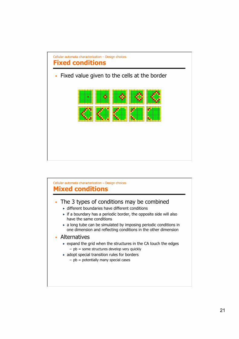
Little changes in the table

§  Even a small change in the rules table can lead to very significant changes in the resulting dynamics �  ex1:

�  ex2:


Totalistic rules (1)

§  Lots of Cas don’t care about the exact disposal of the cells but only about the number of neighbours in a given state �  allows to simplify the transition table

§  Totalistic CA �  only consider the sum of the states of the neighbouring cells

§  « Outer totalistic » CA �  also depends on the current state of the cell concerned

28


Totalistic rules (2)

§  Most of the time, we sum only a subset of the states �  ex: greenberg-hastings = sum of the cells in state 2

�  in the example: –  g(0) = 0 –  g(1) = 0 –  g(2) = 1 –  f(0,0) = 0 –  f(0, x>0) = 2 –  f(1,x) = 0 –  f(2,x) = 1


A 1D totalistic automaton with 3 states

29


Probabilistic rules (1)

§  The new state of the cell depends on: �  the configuration of the neighbourhood �  probabilities associated to the different possible states (the sum of

the probabilities has to be equal to 1) �  The probabilistic choices of the cells are independent from one

another �  The transition function becomes:

–  G verifying

–  in general, G is non nul for only some values

§  important to simulate a number of systems in which the functionning is noisy


Probabilistic rules (2)

§  Example

�  take into account the fact that propagation does not always noccur

�  irregular front but more circular

30


A probabilistic 1D automaton

Cellular Automata - Site UEVE Productionhutzler/Cours/mSSB/CellularAutomata.pdf · Cellular...

Documents

Transcript of Cellular Automata - Site UEVE Productionhutzler/Cours/mSSB/CellularAutomata.pdf · Cellular...