Cellular Automata and ParallelProcessing for Practical

Fluid-Dynamics Problems

H. AbarbanelK. Case

A. DespainF Dyson

M. FreedmanC. Max

D. Nelson0. Rothaus

September 1990

JSR-86-303

This report was prepared as an account of work sponsored by an agency of the United States GovernmentNeither the United States Government nor any of their employees, makes any warranty. express or implied, orassumes any legal liability or responsibility for the accuracy completeness, or usefulness of any information,apparatus, product, or process disclosed, or represents that its use would not infringe privately owned rightsReference herein to any specific commercial product, process, or service by trade name, trademarx, manufacturer,or otherwise, does not necessarily constitute or imply its endorsement, recommendation, or favoring by theUnited States Government or any agency thereof. The views and opinions of authors expressed herein do notnecessarily state or reflect those of the United States Government or any agency thereof

JASONThe MITRE Corporation

7525 Colshire DriveMcLean, Virginia 22102-3481

(703) 883-6997

i -ppT.e ,i. pub*

REPORT DOCUMENTATION PAGE T Form ApprovediI O0M8 No. 07(4-0188

pW&K te",inin burdenl for tis CoificCioE of informsation i t ited to aefeWI ou "0ta OtrcIoome. inciudinq iv tie fm.9or reiro...q instrojoni.m ,tachrnq "ntinq data souc.Vgatha.nq and maintaining fthe data neded. and CORN01011ing and. re*Ce-nq the. coliition of -nformaton 1efld rommntSre9~l n udnetmte~a' re ieno u

,oiptdro,rotormstoe. *nidadir'q *, qqasf1tOes for reducing [PIPS burden. to WosnnAQoa, n*addaarfe,s $vinefen. Oireeorar o nomation, Oinatioms and itecnu. 121 ) W.oenfs HNgqvSV. Suit# 104. Atrnqon. VA 22202-4302. and to thea Office of Manaqcemept and Suoaqvit faoerwora atdaucion Proft (07044188S). Woiasfuosqnoas OC JOS03

i. AGENCY USE ONLY (Leave blank) 2REPORT OAT4 9 3. EPORT TYPE AND DATES COVERED

ISeptember -0, 1994. TITLE AND SUBTITLE S. FUNDING NUMBERS

Cellular Automata and Parallel Processing for PracticalFluid-Dynamics Problems

6. AUTHOR(S) P 53

H. Abarbanel etal

7. PERFORMING ORGANIZATION NAME(S) AND ADORESS(ES) 3. PERFORMING ORGANIZATIONThe MITRE Corporation REPORT NUMBER

JASON Program Office A107525 Coishire DriveMcLean, VA 22102 JSR-86-303

9. SPONSORING. MONITORING AGENCY NAME(S) AND ADDRESS(ES) 10. SPONSORING/ MONITORING

Depatmen of ~j= -AGENCY REPORT NUMBER

JSR-86-303Washington. DC 2

111. SUPPLEMENTARY NOTES

112a. DISTRIBUTION/ AVAILABILITY STATEMENT 12b. DISTRIBUTION CODE

-r,.s report %as prepared as an account of work sponsored by an agency of the United States Goversnent Neither the liability

epresents ma'. as use would not infringe pnnaiely owened rights Reference herein to any specific commercial product.rnicess, or sersicc ns trade name, trademark, mnanufacturer, or otherwise. does not necessarly constitute or imply its

,ndorsemen:. rccormedation. or favoing by the United Staies Govemnment or any agency thereof The views and opinionsai~viors exprcssed herein do not nececssarcy suite or reflect those of the Uruted States Gonemment or any agency, thereof

13. ABSTRACT (Maximum 200 words)

During the 1986 JASON Summer Study a group of JASONs undertook to examine, under thesponsorship of the Department of Energy and DARPA )the utility of cellular automata in physicalscience calculations, especially in fluid dynamics. We expanded the scope ofour study to includeseveral related topics which we concluded would be of some interest to our sponsors. These include:(1j a comparison of cellular automata (CA) techniques to "conventional" methods of solving thepartial differential equations of fluid dynamics or other physical si'tuations, and (2) the utility andstatus of using parallel or concurrent processing machines for doing either CA or conventional fluidscalculations.

14. SuBJ ECT TERMS 1S. NUMBER OF PAGES

cellular automata, vlsi chip, impressible fluid algorithrnns; ___________

two, three, or four dimensions; octogonal quasilattice 16. PRICE coDE

17. SECURITY CLASSIFICATION 13. SECURITY CLASSIFICATION 19. SECURITY CLASSIFICATION 20. LIMITATION OF ABSTRACTOF REPORT I OF THIS PAGE OF ABSTRACT

UNCLASSIFIED UNCLASSIFIFD IUN('LASSIFIFI) SAR

NSN 7547' '-5500 Stanoard Fort" 298 (ROV 2-89)"V5Coom Or A*NP6 %to 1)9. I

Contents

1 INTRODUCTION 1

2 CELLULAR AUTOMATA RULE FINDING FOR USE IN3-D FLUID DYNAMICS 52.1 3-D Cellular Automata ...................... 12

3 A VLSI CHIP FOR A CELLULARAUTOMATA MACHINE 173.1 Introduction .. .... .. ... ...... ....... .. .. 173.2 Computational Cell for 4-D Rules ................ 19

4 GENERAL COMPARISON OF CELLULAR AUTOMATAAND CONVENTIONAL FLUID-DYNAMICALMETHODS 274.1 Cellular Automata: Potential Advantages ............ 274.2 Cellular Automata: Disadvantages ............... 274.3 Conventional Methods: Advantages ............... 284.4 Conventional Methods: Disadvantages ............. 284.5 Comparison on the Basis of Computational Work ........ 29

4.5.1 Number of Grid or Lattice Points ............ 294.5.2 Number of Bits per Lattice or Grid Point .......... 334.5.3 Number and Speed of Operations per Timestep .... 364.5.4 Number of Timeteps ................... 384.5.5 Ease of Adapting to a Parallel Computation Environment 394.5.6 Overall Comparison of Computational Effort ....... 40

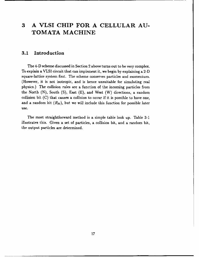
5 QUASILATTICES FOR CELLULAR AUTOMATON FLUIDCALCULATIONS 475.1 Introduction . . . . . . . . .. . . . .. .. .. .. . .. . . .. 475.2 Octagonal Quasilattices ..................... 495.3 Icosahedral Quasilattices ..................... 59

6 COMPARISON BETWEEN CONVENTIONAL KINETICTHEORY AND CELLULAR AUTOMATA DERIVATIONSOF HYDRODYNAMICS 69

ill

6.1 Introduction ............................ 696.2 Equations for One Particle Distribution Function .. .. .. .. 70

6.2.1 Molecules .. .. .. ... ... ... .... ... .... 706.2.2 C.A. .. .. ... ... ... .... ... ... ... .. 71

6.3 Macroscopic Conservation Laws. .. .. .. ... ... ...... 726.3.1 Molecules .. .. .. ... ... ... .... ... .... 726.3.2 C.A. .. .. .. .. ... ... .... ... ... ... .. 73

6.4 The Euler Equations. .. .. .. ... .... ... ... .... 746.4.1 Molecules .. .. .. ... ... ... .... ... ..... 746.4.2 C.A. .. .. .. .. ... ... ... .... ... ... .. 75

6.5 The Chapman-Enskog Expansion .. .. .. ... ... ... .. 766.5.1 Molecules .. .. .. ... ... ... .... ... .... 766.5.2 C. A. .. .. .. .. ... ... .... ... ... ... .. 78

6.6 Conclusion. .. .. .. .. .... ... ... ... ... ... .. 80

7 PACKING A PLANAR LATTICE 83

Accession For

V0 -N~~tTIS G-RA &IDTlC TAB0

uniannounced 0lJustifioatio Sponsoring/Monitoring agency was U. S.

Dept. of Energy, office of Program

By Analysis/ER-32 . Washington, DC 20585.Di tributiol/AvailabilitY Codes Dist. "A" per Charles mandelbaumn. Office

jAvail and/or of Program Analysis/ER-32. U. S. Depart-

ctt Special ment of Energy/ER32 eahngoD20585.

VHG 11/07/90

iv

1 INTRODUCTION

During the 1986 JASON Summer Study a group of JASONs undertook toexamine, under the sponsorship of the Department of Energy and DARPA,the utility of cellular automata in physical science calculations, especially influid dynamics. We expanded the scope of our study to include several relatedtopics which we concluded would be of some interest to our sponsors. Theseinclude: (1) a comparison of cellular automata (CA) techniques to "conven-tional" methods of solving the partial differential equations of fluid dynamicsor other physical situations; and (2) the utility and status of using parallelor concurrent processing machines for doing either CA or conventional fluidscalculations.

To assist our study we hosted a series of external briefers who kindlygave of their time and expertise. On the subject of CA and applications tofluid dynamics we heard from Dr. Jay Boris of the Naval Research Labo-ratory who spoke on "Cellular Model for Tasking and Correlation," Dr. T.Toffoli of MIT who spoke about "Primitives of Computation and of Physicsas Applied to Cellular Automata," Dr.Gary Doolen of the Los Alamcs Na-tional Laboratory who addressed us on the topic of "Lattice Gases," Dr. S.Wolfram of the University of Illinois speaking on "CA and Hydrodynamics,"Dr. S. Omohundro of Illinois speaking on "Applications of the ConnectionMachine Architecture," Dr. B. Nemnich who spoke on "The ConnectionMachine," and Dr. P. Collela from the Lawrence Livermore National Lab-oratory speaking on "Multiple Scale Problems in Hydrodynamics." On thesubject of parallel processing we heard, in addition to the talks of Nemnichand Omohundro, from Dr. J. Barhen of Oak Ridge National Laboratory on"Hypercube Computer: Architecture and Algorithms for Advanced Applica-tions," and from Dr. J. Fier of the AMETEK Computer Research Divisionon "Hypercube Architecture and Applications." To all these workers in thefield we give our thanks for their assistance.

The work reported on in the present study was begun at JASON in thesummer of 1986. Since that time there has been a considerable maturation ofthe field of cellular automata. The reader desiring further background mayrefer to two excellent review volumes:

21

1. Complex Systems volume 1, no. 4 (August 1987); this volume is basedlargely on presentations of a workshop held in Santa Fe, NM in Octoberof 1986.

2. Lattice Gas Methods for Partial Differential Equations, edited by G.Dollan et al. (Addison-Wesley, N.Y., 1989).

Our own work has been organized along the following lines:

" We have examined the relationship, in terms of effort and efficiency, ofdoing fluid dynamics calculations using cellular automata versus moreconventional spectral or finite difference methods. We conclude thatcellular automata calculations are likely to be competitive with stan-dard finite element or spectral methods for the Navier-Stokes equationsprimarily for low Reynolds numbers and Mach numbers. An exceptionto this may occur in complex geometries or with boundary conditionswhere conventional methods are often quite difficult.

" We have reviewed the derivation of ordinary Navier-Stokes Newtonianfluid dynamics from kinetic theory and compared it to the derivation offluid dynamics from CA. Only for low Mach numbers do we have someconfidence that fluid dynamics is being simulated in these calculations.

" We have looked into two schemes for carrying out CA calculations inthree dimensions-one uses the notion of tiling or covering 3-D spacewith a quasi-periodic lattice of Penrose type, and the other investigatesthe idea of doing CA computations in dimensions larger than three andthen projecting the results back into three dimensions. In each casethe issue is achieving enough structure in the underlying covering of3-D space to assure correct tensorial characteristics of the quantitiesentering the Navier Stokes equations.

" We have formulated in an abstract fashion the problem of represent-ing in a physical 3-D computational structure 2-D highly parallel CAcomputations.

Perhaps it is useful to define what we mean by some of the terms usedalready in this introduction, especially those which will appear throughoutthe report. First of all, we need to address the meaning of cellular automata.

2

The idea of cellular automata is that by using very restricted informationon the position and velocities of individual particles in their microscopiccollision and interaction one can, nonetheless, arrive at a good representationof macroscopic dynamical equations such as the Navier-Stokes equations,since the latter involve averaging over larger numbers of individual particles.Fr- thermore, the averaging is over space and time scales large compared tothe microscopic dynamics, so one might think that a crude representation ofthe latter could result in realistic and acceptable macroscopic physics. Thegenerality of macroscopic equations such as the diffusion equation or the fluiddynamics equations which are parametrized by a few transport coefficientsin which all the microphysics is buried would also support this point of view.The key notion of CA, as opposed to the ideas of molecular dynamics, isto very crudely represent each individual particle motion. Crude here meansgiving the position on a simple lattice covering the space of interest and givingthe velocity as one of a few choices such as plus or minus unity. In otherwords, by representing the phase space coordinates of individual particles byonly a few bits of information, one hopes that the aggregate average neededto construct the macroscopic velocity or density is accurately and efficientlycomputable.

3

2 CELLULAR AUTOMATA RULE FIND-ING FOR USE IN 3-D FLUID DYNAM-ICS

There is some difficulty in finding simple cellular automata dynamicsin three dimensions which adequately simulate the Navier-Stokes equation.From a purely formal (i.e., nonphysical) point of view, there are a numberof ways of overcoming these difficulties, and as we will show, many of thepurely formal procedures have a straightforward physical interpretation. Asa consequence of these investigations, we can present what appears to be thesimplest, and most straightforward, cellular automata simulation of 3-D fluidmotion.

To begin, whether in two- or three-dimensions, our lattice sites will al-ways be the points with all integer coordinates, i.e., the usual integral lat-tice. In addition are given a collection of vectors e1, e2, ... eN each vectorbelonging to the lattice. In the list, a given vector may occur repeatedly.At any instant of time, the total state of our automaton is described byan N-dimensional vector of zeros and ones given for each lattice site. Inother words, the state of our automata at time t is described by specifyingA,(x, t), a = 1, 2,... N, and x running through the lattice sites. For fixed xand t, the vector [A,(x,t),A 2(X,t), ... ,AN(X,t)] is called the state vector atsite x, time t.

The evolution or dynamics in our automaton is given a. follows:

A(X,t+ 1) = F,,a = 1,2... N,

where each F. is a fixed function of the state vectors of the automaton at timei at sites in a fixed neighborhood of x. What we mean to say here is simplythat the rule for advancing in time is the same function of neighboring statesat each site and all times. You may think of the Fa as including both thecollision laws and the motion of the more conventional description of cellularautomata, but in general they have no such simple physical description.

In order to bring out clearly what the essential properties of the dynamicsare, we will write:

Fa = A(x-ea,t)/fl (2-1)

5

and demand that identically for all total states of the automata at time t,we have:

no = 0 (2-2)a

eafl. = 0. (2-3)a

The I's are simply the measure of the difference in the dynamics of theautomaton from straight collisionless motion of the particles. They are rarelymentioned specifically for most of the familiar constructs, but they do playan important formal role, as we shall see momentarily. It is quite easy tosee that conditions in Equation (2-2) are met, as a matter of fact, for thefamiliar square and hexagonal lattice fluid dynamics constructs, without evenspecifically bringing in the QVs.

For our original list of vectors e', we are going to insist that all the tensorsa a

Ei eO, e 0 ea, Ea e e & ea and ei e ,e ea(ea be isotropic.

Thus, for example, if we take in two dimensions the 20 vectors: (±1, ±1)once each, (±1,0) 4 times each, and (0, ±1) 4 times each, we satisfy theisotropy requirements. In three dimensions, we may take the 24 vectors(±1,±1,0) once each, (±1,0, 0) twice each, (0, ±1,0) twice each, and (0, 0, ±1)twice each to satisfy the isotropy requirements.

In general, for a given set of e's, it seems quite easy to produce a largenumber of Fa's satisfying the requirements (2-1) and (2-2) above. Subse-quently, we will produce Fe's for the e's described in the paragraph immedi-ately above.

Suppose we assume that our automata locally equilibrate in space. De-note by E the admittedly vague notion of expectation operator for the localspatial equilibration, and put fa(x,t) = E(A,(x,t)). By virtue of the re-

quirements (2-1) and (2-2), we obtain:

Efa(xlt+ 1) = E f.(Xea, t) (2-4)

a a

Eeafa(x,t + 1) = Eefa(..X-ea,t). (2-5)a a

6

Denote n(x,t) = E.fa(x,t) and n(x,t) u(x,t) = Eefa(X,t). In thecontinuum limit of long times and large lattices, the equations above become:

S-+V-nu = 0 (2-6)

-j(nu) + Ee(e.Vf.) = 0. (2-7)a

It is convenient to refer to n(x, t) as particle density, u(x, t) as average ve-

locity, and nu as momentum density. With this convention the requirements(2-1) and (2-2) provide for conservation of particle number and momentum.For if we pick an initial state for the automaton in which only finitely manyof the state vectors are non-zero, we get from (2-1) that

n(xt + 1) = n(xt)

or in the continuum hrmit

d J n(x, t)dx- = 0.

Similarly (2-2) gives conservation of momentum in time.

Analogously, if the initial state for the automaton is periodic in the spa-tial variables, so also are subsequent states and with the same periods, andthe total particle number and total momentum over a periodic rectangularparallelogram or parallelepiped is conserved in time. Imposing periodocityis equivalent, of course, to running the dynamics on a 2- or 3-D torus.

At this point, we make the bold assumption that the functions fa(x, t)

can be determined from the equilibrium parameters u(x, t) and n(x, t) bya Chapman Enskog expansion. Arguing just as in Wolfram1 we end withNavier-Stokes like equations for a continuum fluid.

For the rest of this section, we are going to show that, at least in somecases, the formal procedures described above really work. Along the way, wewill produce a particularly simple way of running 3-D fluid dynamics at the

cellular automata level.

We will begin with a 4-D cellular automaton with the lattice sites beingas usual the points with all integral coordinates. Lattice points are labelled(x,y,z,w). We take the sublattice of integral points for which the coordinate

7

sum is even, which is of index 2 in the full integral lattice. This lattice isconnected with a very interesting tessalation of tUe 4-D space, but this doesnot concern us here. In the sublattice we take all points of least nonzerodistance from the origin, these being precisely the 24 vectors: (±1, ±1,0, 0)

and its permutations. These 24 vectors are the list ea, a = 1,2,..., N = 24.It is easy to verify that the requirements of isotropy are met by this list, that

is, for example:

E(,a)(,a)(e' ) (,a), = i3'kt + bikbit + bitbik.a

There are a number of available scattering laws to give a good momentumscramble, e.g.:

A) Binary: (1,-1, 0, 0) + (-1, 1, 0, 0) - (0, 0, 1,-1) + (0, 0,-1, 1)

B) Ternary: (1, -1, 0, 0) + (0, 1, -1, 0) + (-1, 0, 1, 0) - (-1, 1, 0, 0) +(0, -1, 1, 0) + (1, 0, -1, 0)

C) Ternary: (1, 0, 0, -1) + (1, 0, 0, 1) + (-1. 1, 0, 0) 4--* (0, 1, 0, 1) + (0,

1, 0,-i) + (1,-1, 0, 0) and

D) Ternary: (1, 0, 0,-1) + (1, 0, 0, 1) + (-1, 1, 0, 0) +-+ (1, 1, 0, 0) + (0,1, 1, 0) + (0, -1, -1, 0)and so avoid undesirable conservation laws. If we run a 4-D cellular automa-ton with a suitable collection of such scattering laws on the integral lattice,

there is however one inevitable conservation law, which will not concern us inthe applications we make. This arises simply from the fact that the dynam-ics takes place in two uncoupled sets, namely the sublattice of points whose

coordinate sum is even and the coset of points whose coordinate sum is odd.

The application of this 4-D cellular automaton to 3-D problems is now

quite straightforward. Take any initial state in the 3-D section (x,y,z,w = 0),and extend it to 4-D by repeating it in every section w = k, k an integer. If we

have deterministic scattering laws, then throughout the evolution all sectionsw = k remain the same as the section w = 0. [Even if we have probabilistic

scattering laws, we can maintain the identity of sections by insisting that thechoice made at a site (x,y,z,0) in the section w = 0 be repeated at all sites

(x,y,z,w)l.

8

All sections remain the same, thus macroscopic particle density, momen-tum density and average velocity vector are independent of w. since we getthe same average over a region and any translation of the region along thew-axis.

The even sublattice and its colattice are now coupled together becausethe sites (x,y,z, even) and (x,y,z, odd) have the same state.

If we now look at the 4-D Navier Stokes equation which our 4-D automa-ton is presumably simulating, then since density and momentum density arenot functions of w, the projection 7ru of the velocity vector u into the sectionw = 0 together with the original density n, satisfy a Navier Stokes like systemin 3-D.

Since the sections w = k remain the same throughout the evolution ofthe 4-D automaton, the dynamics can be fully described in the section w =0. How do we do so? We need to describe the state at each 3-D site witha 24 bit vector, corresponding to presence or absence of a particle headedin direction ea;a = 1,2,... ,24. Since we will be concerned only with theprojection of the 4-D momentum into the section w = 0, we project the 24vectors ea to get:

(±l, ±1, 0) once each(±1,0, ±1) once each(0, ±1, ±1) once each(±1,0, 0) twice each(0, ±1, 0) twice each(0,0, ±1) twice each.

The versions i the projected vectors which occur twice are to be labelled; wecall one spin plus, the other spin minus, depending on the sign of the invisible4th coordinate. The scattering laws such as (A), (B), (C), (D) describedearlier are replaced by their versions with the last "oordinate suppressed,but the vectors therein labelled spin plus or minus as required. The 3-Dmotion after scattering takes place along the 24 projection of the vectors F a.

Here we have precisely what was described only as a possibility earlier,namely a 3-D Navier Stokes simulation using some vectors ea repeatedly. The3-D isotropy is obvious.

9

The 2-D simulation using 20 vectors, described earlier, can be simulatedby projecting once more, into the section z = 0. It is rAatively easy to seethat the four rest particles arising from the projection of (0,0, ±1), can bedispensed with altogether, but we do not go into details.

As matters currently stand, we can run our 3-D Navier Stokes simulationwith a 24-bit vector to describe the state at each site. We want to argue nowthat 24 can be reduced to 18. To do so, we return to our 4-D simulation, withall sections w = k, k an integer, the same. Suppose for the moment that thestate vector at each site in the section w = 0 is reflectively symmetric. By thiswe mean that if one of the particle directions such as (1, 0, 0, 1) occurs, soalso does (1, 0,0, -1). This being the case, the state vector can be describedby an 18 bit vector. Suppose also that the zattering rules we choose to useare reflectivity symmetric. By this we mean that for every scattering law,the law obtained by changing the signs of last coordinates is also a scatteringlaw we use. (With some care, probabilistic scattering laws can be handled).All this being so, it is easy to see that in the evolution of the 4-D automata,the section w = 0 remains reflectively symmetric, and so the 3-D dynamicsneeds only 18 bits per site. At the same time, we must assure ourselves thatwe have enough applicable scattering laws to avoid undesirable conservation

laws. It is clear that we will not succeed by using only those vectors whichoccur singly. But the purpose of our writing down scattering laws (C) and(D) earlier was to persuade the reader now that enough scattering survives,these being two instances of scattering laws in which the spin plus and spinminus directions occur in pairs. Actually, a binary law, such as (1, 0, 0,

+1) + (1, 0, 0, -1) ( (1, 1, 0, 0) + (1, -1, 0, 0), will eliminate unwantedconservations.

It is interesting to note that in running a 4-D reflectively symmetric cellu-lar automaton with all sections w = k the same, the macroscopic momentum

density has no component in the direction of the w-axis.

Now that we are done describing our 3-D simulation, it all seems quitetrivial. We have simply reversed a standard device in fluid dynamics. If,for example, one wishes to describe a 3-D planar flow about a cylindricalobstacle, one reduces to a 2-D problem. We have, perversely, taken a 3-D problem and imbedded it in a 4-D hyperplane flow setting, to gain theadvantage of the useful lattices existing in four dimensions.

10

There is another 4-D sublattice of the integral lattice which offers somepromise. Essentially the dual of the sublattice considered earlier, it consistsof points all of whose coordinates are even, or all of whose coordinates areodd. It is of degree 8 in the full integral lattice. The vectors to consider inthis instance, 24 in number also, are

(±2, 0, 0, 0) and its permutations and

(±,+1, ±1, ±1).

These vectors give the desired isotropy, and projecting into w = 0 givestwo rest particles, 8 particle directions which occur twice, and 6 particledirections occurring once. The rest particles can be eliminated; runningthe remainder demanding reflective symmetry as before will give us a 3-D simulation requiring a 14 bit vector to describe the state at each site.Scattering laws such as

(1111) + (111 - 1) + (-2000) -, (-1111) + (-111 - 1) + (2000)

will give us some momentum scramble, but we do not appear to have ananalogue of the very useful scattering law (D) used in the earlier lattice.Without such analogue, the total number of particles in all of the directionsgiven by the 8 paired spin plus and spin minus directions is conserved, andthis gives us a conservation law. The use of higher order scattering laws caneliminate conservation.

The fact that the 3-D dynamics takes place in 4 uncoupled colatticespresents no difficulties; restrict one's attention to the sublattice: all coordi-nates even, or all coordinates odd.

It is appropriate to describe at this point what we feel is the right way tosearch for conservation laws. Recall that there is an assumption underlyingthe whole discussion of cellular automata, namely that particle number andmomentum are the only conserved quantities.

Now we suppose that the automaton dynamics is broken into two parts,the applications of the scattering laws followed by the lattice motions. At aninstant in time we have a state vector A(x, t) which after scattering becomesA'(x, t), followed by motion to neighboring sites, so that Ao(x, f+ 1) = A'(x-ea , t). Now suppose there is a vector v such that

EvaAa(x, t)= Ev°A.(x,t),

a a

11

no matter what x and t, and such that also E. voA.(x, t) is not identically

zero. Then we have a particle number conservation law, since now

VaA(x,t + 1)= vAo(x - e.,t).a

Integrating over all space and taking expectations yields

J v.- f (x, t)dx- =f v.- f (x, t + dx

which is not the usual conservation law if v • f(x, t) is not a scalar multiple

of n(x,t).

A law different from the usual momentum conservation law would arisefrom a vector v such that

ZVae'A (x, t) = Zvae AA(x,t).a a

On taking the dot product of the last with a fixed arbitrary vector, we wouldfind a particle conservation law of the sort considered just above, so it sufficesto search for particle number conservation laws. As noted above, these arisefrom vectors v orthogonal to A(x, t) - A'(x, t) for all possible x and t.

2.1 3-D Cellular Automata

We will now discuss in greater detail some of the technical issues involved

in efficient use of 3-D cellular automata for simulating fluid flow, confiningour attention to the two kinds of automata described in Section 2. The firstof these is associated with the 4-D lattice of integral points whose coordinatesum is even and for which we pick lattice motions corresponding to the 24directions (±1, ±1,0, 0) and its permutations, this choice assuring sufficientisotropy of the flow to mimic the Navier-Stokes equations. The second choiceis the lattice of integral points for which all coordinates are even or all are odd.

In this case we pick 24 lattice motions associated to the vectors (±2, 0, 0, 0)and its permutations and (±1, ±1, ±1, ±1), enough again to insure isotropy.

In both cases we are going to use the 4-D automaton to simulate 3-Dproblems. This is effected by choosing initial conditions in the section w =0, and repeating them in all the other sections w = k. If the scattering lawused at the site (a, b, c, k) is the same for all k at each fixed instant in time,

12

then all sections remain the same in the evolution of the automaton, and itis enough to simply follow the evolution in the section w = 0.

In order to further reduce the computational burden, the following usefuldevice, already pointed out in Section 2, if a particle is needed in direction(a, b, c, d), there is also one headed in the direction (a, b, c, -d).

For the first lattice mentioned above, this convention permits the stateat a 3-D site to be described by an 18-bit vector. For the second, the stateat a site requires 16 bits. But since it is easy to see that the effect on theevolution of the automaton arising from the pair of directions (0, 0, 0, ±2), ifthese are not used in any scattering laws, is irrelevant and does not createany unwanted conservation in the 3-D section w = 0, the number of bitsnecessary to describe the state at a site can be reduced to 14.

For the second lattice the pair of directions (0, 0, 0, ±2), which look likerest particles from the 3-D point of view, have simply been dropped. Foreither lattice, a pair of directions such as (a, b, c, 1) and (a, b, c, -1), bothof which occur at a site, or neither, is called a "married pair."

For both lattices, a variety of scattering laws are available, much more sothan in the simple 2-D hexagonal lattice, even with the restrictions createdby the married pairs. The problem, as we see it, is to have a rich enoughcollection of scattering laws to eliminate any undesirable particle or momen-tum conservation laws, but not so many that the computational logic at asite becomes unwieldy or too slow.

Part of the difficulty in achieving this goal is a consequence of the obser-vation that some randomization is needed in applying scattering laws. Forexample, if the pair (1, 1, 0, 0) and (-1, -1, 0, 0) are present at a site, theycan be replaced by any other velocity vector pair which sums to zero. Howshall the choice be made? Similarly, we may have scattering laws:

(A) (1, 1, 0, 0) + (-1,-1, 0, 0) - (1, 0,-1, 0) + (-1, 0, 1, 0)

(B) (1, 1, 0, 0) + (1,-1, 0, 0) 4-- (1, 0, 1, 0) + (1, 0,-1, 0).

If all three velocity vectors on the left are present at the site, and none ofthose on the right, which of the two laws should be applied?

13

Recall that the ultimate macroscopic features of the flow arc to be ob-

tained by averaging over suitable sub-regions of the 3-D grid. If the scatteringis very limited, or not always applied when available, then mean-free-pathswill be quite long; consequently the suitable sub-regions of the grid will haveto be undesirably large. On the other hand, attempting to put in all thescattering available will require intricate combinatorial decisions, and a fair

amount of randomization.

For these and other reasons, it is desirable to keep the scattering lawsas simple as possible. The simplest scattering laws are, of course, binaryscatters, and physically these are the most likely to occur. It is fortunatethat for the first of the two lattices described earlier, with 18 bits per site forthe state vector, the use of binary scattering only suffice.

We describe the situation here in a little more detail now. We can inter-change any of the four following pairs

1 1 0 0 -1 -1 0 0 1 0 1 0 M 1 0 -1 0

(I) -1 -1 0 0 1 1 0 0 1 0-1 0 1 0 1 0

or any of the following three pairs

(m 1 1 0 0 1 0 1 0 1 0 0 1)(i) 1 -1 0 0 ) (1 0 -1 0 ) (1 0 0 -1

and analogously,

-1 1 0 0),0 1 1 0 0 1 0 1IIi - 1 0 0 0 1 -1 0 ) (0 1 0 -1 )

(V 1 0 1 0 0 1 1 0 0 0 1 1 ), an d(I)(1 0 1 0 )'0 -1 1 0 )'0 0 1 -1

(I) gives us 6 binary scatters, (II) to (VII) give us 3 binary scatters each,for a grand total of 24 scatters. Notice that these scattering laws meet the

restriction imposed by the married pairs. It is also possible to verify thatthese binary laws are sufficient to avoid undesirable conservation laws (asdescribed in Section 2); it is the exchanges offered by (II) through (VII)which mix up the "married pairs" with the "single" velocity vectors.

We have not investigated the question of how many of the binary scatterscan be dropped while still avoiding conservation laws, though it is clear thatsome can be. We could, for example, rather than permit the interchanging

14

of all the pairs of (I), interchange only pair 1 with pair 2, 2 with 3, ... , pair 4with pair 1. Even with limitations such as this, the question of which inter-change is to be made has to be decided with a randomization; if the secondpair is present, and not the first or the third, which of the two interchangesshould be effected?

It is problematic whether using a thin set of the binary scattering laws,big enough to avoid conservation, will give us results as favorable as usingthem all. We do not see any particular advantage to limited use, and aregoing to proceed on the basis of using all the binary laws, and on somethinglike an equal footing.

Now we describe one scheme for using all of the 24 laws of the first lattice.The laws are labeled from one to twenty-four. A random number generator,somewhere on the side, picks a number between one and twenty-four, onefor each site, and applies the selected scattering law if it can be applied;otherwise no scattering takes place. The random choice of scatter at eachsite is followed by motion of particles to neighboring sites, and then repetitionof the procedure.

In practice it may be desirable to have the random selection of the integerbetween one and twenty-four other than uniform. Since there are a very largenumber of fast methods for generating random numbers with frequencies, wewill not go into these questions here. There is, nonetheless, quite a large bit ofrandomization-one generator for each site. Possibly the randomization canbe carried out intrinsically as follows: use the bits, and their complements,in the far field of a site to generate the random number at the site. Thereare obvious risks and deficiencies in this procedure, however.

For some purposes, the method outlined above will not effect scatteringwith sufficient frequency, for an available scattering law at a site has roughlya probability of 1/24 of taking place. At the cost of slowing the proceduredown, a straightforward alternative is available as follows. After the firstchoice of scattering law is made and applied if possible, and before the particlemotion to neighboring sites, a second independent choice is made of binaryscatter and applied if possible. This may be repeated as many times asnecessary before motion. An attractive feature of this scheme is that thenumber of repetitions may be settable by the program. Whether the schemeis any better than running the simulation faster with only one randomization

15

per motion depends on the time trade-off for scattering steps compared to

motion steps.

There is still another way of proceeding which in a sense eliminates the

need for randomization. One may simply choose, once and for all, at each

site in the field one of the 24 binary scattering laws, the choice to be madeas randomly as possible. This is probably the cheapest and fastest way to

simulate, though it might be useful for some purposes if the fixed random

allocation of scattering laws to sites could be easily changed.

So much for the first lattice. The second lattice has a smaller state vectorat the site, but is considerably poorer in scattering laws. With the restric-tion imposed by the "married pairs," there are only three binary scatters-interchange any of the following three pairs

2 0 0 0 0 2 0 0 0 0 2 0(I -2 0 0 0 ' (0 2 0 0 ' (0 0 -2 0 '

none of which mix up married and singles. There are no ternary laws; thereare, however, 24 special quaternary laws of which a general example is

(1,1,1,1) + (1,1,1,-1) + (-1,-1,-1 -1) *-+

(2,0,0,0) + (-2,0,0,0) + (0, 2, 0, 0) + (0,-2,0,0)

and these 24 together with the three of (I) eliminate unwanted conservation.

This lattice with the 27 scattering laws above can be used along any of

the lines described for the first lattice, though it is not at all clear what the

relative frequency of scatters coming from (I) with those coming from (II)should be. In general, especially in instances in which overall density is fairly

large or fairly small, it is going to be difficult to use (II) and its ilk. Sincewithout (II) the marrieds and singles are never mixed, it seems clear that

somewhat greater emphasis must be put on finding applications of (II).

In the final analysis, the performance in practice of either lattice, along

any of the lines described above, must be studied by actual computer simula-tions. A great deal will depend on the size of the region over which averages

are taken in order to obtain macroscopic estimates, on details of the scatter-ing laws used, and on particle density.

16

3 A VLSI CHIP FOR A CELLULAR AU-TOMATA MACHINE

3.1 Introduction

The 4-D scheme discussed in Section 2 above turns out to be very complex.To explain a VLSI circuit that can implement it, we begin by explaining a 2-Dsquare-lattice system first. The scheme conserves particles and momentum.(However, it is not isotropic, and is hence unsuitable for simulating realphysics.) The collision rules are a function of the incoming particles fromthe North (N), South (S), East (E), and West (W) directions, a randomcollision bit (C) that causes a collision to occur if it is possible to have one,and a random bit (RN), but we will include this function for possible lateruse.

The most straightforward method is a simple table look up. Table 3-1illustrates this. Given a set of particles, a collision bit, and a random bit,the output particles are determined.

17

Table 3-1

INPUT NSEW C RN OUTPUT NSEW0000 00000001 00010010 00100011 0 - 00110011 1 - 11000100 - - 01000101 - - 01010110 - - 0110

0111 - - 01111000 - - 10001001 - - 1001

1010 - - 10101011 - - 10111100 0 - 11001100 1 - 00111101 - - 1101

1110 - - 11101111 - - 1111

Now consider a 'factored' solution to the same problem. Only head-on colli-sions can result in scattering and if scattering is to occur, then there must bean output channel for each particle to occupy. Thus there are two 'scattering'rules:

1) N.S.E,. W C E EW

2) I.S E. W.C .. N. S.

The first rule can be read as

"If there is a particle from the North, and a particle from theSouth,

and no particle from the East, and no particle from the West, and

a collision is to occur, then send a particle out to the East andsend a particle out to the West."

18

The enabling condition parts of these rules are simply implemented by'and' gates.

Next we must decide which rule to employ if both should be enabled.(Of course, in our example this can never actually occur, but it will occur inmore complex systems.) We will employ a priority encoder to choose a rule,with a dynamic priority assignment by the random bit.

Finally, the chosen rule will select which output channels to block andwhich output channels to inject particles into.

The complete circuit is illustrated in Figure 3-1. It is, of course, morecomplex than a simple table look-up approach for this very simple system.However, it illustrates the method we intend to use to implement the 4-Dcellular automata scheme.

3.2 Computational Cell for 4-D Rules

The 4-D case has a total set of 24 incoming particles but some (6) arepaired, so only 18 bits are needed to specify the incoming and outgoing parti-cles. In addition there are 66 rules, so that seven input priority specificationbits are needed to randomize rule selection. These will be decoded to theone in 66 priority selection bits. The 'C' bit (C) suffices to determine if anallowed collision will occur.

The straight-forward table look-up scheme will no longer work efficientlyas a table of 18 * 2 * *(18 + 7 + 1) - 10' bits is needed. So we will employ the'factored' approach illustrated above. The computational node to accomplishthis is shown in Figure 3-2.

The rule enabling conditions will be calculated in the 'AND-plane' of aPLA (programmcd logic array). Thus we input the collision enabling bit andall of our particle signals, as well as the logical complement of each. Thisis some 38 total input signals. The result is 66 rule enable requests (R).Figure 3-3 illustrates the connections for the 'AND-plane.' From Figure 3-3,it is easy to count that there are 282 transistors needed to implement theconnections. A few more (,, 100) will also be needed to function as inverters,drivers, etc., for a total of about 500 transistors.

19

RANDOM PRIORITY ASSIGNMENTRN)

REQUEST

RULE 1 GRANT RULE 1

C

REQUEST 3RANT RULE 2

NN

SS

--- Ei

w W,

COLLISION RULES PRIORITY SELECTION SWITCH PARTICLES

Figure 3-1. "FACTORED" Computation Cell.

20

To Neighbors

Stored State

(Lattice Pts)

I Swich H Prioity H AndPriority PLA-----

Figure 3-2. A computational node for the VLSI chip.

21

MARRIAGES INTER-GROUP OUTER-GROUPAND HEAD-ON MIXING HEAD-ONDIVORCES COLLISIONS COLLISIONS COLLISIONS

1 2 3 4 5 6 7 8 9 10 1112 13 14 15 16 1718 192021222324252627282930313233

00o + 1ii T . ...... .. .0 00- 1 T

0+0

0-0

0--00

0 - + 1 1 1 .. ..

0++

+) -0-F:.R E l i e i ii. e o I InI0 - - 1: ; A .. .I: : . . . .

-+0- 1 ; T: ::I ... I

++0 """ ""'''

Figure 3-3. AND-plane' of Rule Enable Signal Generation Circuit. (The complement of each inputsignal appears in the row next to the signal.)

22

The next step is to select (randomly) a rule to fire. We will decode theseven random input bits into 66 signals to control the 'AND-gates' of thepriority circuit. This will require about 500 transistors.

If a simple extension of the priority circuit of Figure 3-1 is employed, itwould require three gates and two inverters per stage, or about sixteen tran-sistors per stage. This would be about 1000 transistors for the simple prioritycircuit. Such a priority circuit would be far too slow, and if pipelined wouldhave too much latency. So a 'carry-look-ahead' scheme will be employed. Itwill require about 1200 transistors total if full look-ahead is employed usinga gate fan of about 4. This combined with modest pipelining would requireabout 1500 transistors total. So we will assume this number.

The output switch circuitry will require 36 gates or about 150 transistors.

Thus we see in summing up that the factored circuitry will require about3000 transistors per computation node.

If one-half the chip is dedicated to computation circuitry and one-halfto memory (to store the virtual node state) then about 8 x 8 (64) realcomputation nodes/chip is about the limit that ,.u,,i re expccted for near-term VLSI technology (see Table 3-2"

Tabie .1-1

VLSI TECHNOLOGY (CMOS)

Today ] in about 5 years- cm 2 active area - cm 2

- 200 pins - 400 pins-, 1 Mbit DRAM -, 4 Mbit DRAM- 50K 'Random' transistors - 200K Tran.-- 10 nsec internal clock - nsec-, 80 nsec external drive - nsec

These nodes are laid out as illustrated in Figure 3-4.

The performance of the proposed 'ldttice gas computer' is now easilyestimated (see Table 3-3).

23

To~

Too

Mux A Computational Node

Figure 3-4. Layout of nodes on Lhe VLSI chip.

24

Table 3-3

PERFORMANCE ESTIMATES

FuturePresent Day (5 years)

512 lattice points

64 nodes/chip

106 chips

32K lattice points/chip

3 x 1010 lattice points TOTAL z 1011

10 nsec update rate

64 x 10' updates/chip/sec

1016 updates/sec 10"'

About 106 VLSI chips is the limit for a single computer system (modernlarge scale supercomputers have about 3 x 10' chips). At 512 lattice pointsper node, 64 nodes/chip and 106 chips, up to 3 x 1010 lattice points may befeasible. With a 10 nanosecond update rate, 64 x 108 updates per chip and106 chips yields an update rate of , 1016 per second.

Advances in VLSI technology over the next five years will allow ; 3 timesthe number of lattice points and , 10 times the internal clock rate to yield; 1011 lattice points updated at the rate of zt 1017 updates per second.

25

4 GENERAL COMPARISON OF CELLU-LAR AUTOMATA AND CONVENTIONALFLUID-DYNAMICAL METHODS

Before looking in detail at the computational requirements for cellularautomata and conventional fluid dynamics, we first attempt to summarizesome of their relative advantages and disadvantages in a more general way.

4.1 Cellular Automata: Potential Advantages

Cellular automata have the nice properties of elegance, in the sense thattheir microphysics is immediately transparent, and of local simplicity. They

are more immediately suitable for parallelization than conventional fluidmethods, and they lend themselves to the design of custom computer ar-chitectures which may give very large increases in speed relative to conven-tional multipurpose machines. In addition, because of the "modular" natureof their geometry, they may be able to handle some types of complicatedboundary conditions more readily than conventional fluid techniques.

4.2 Cellular Automata: Disadvantages

On the other hand, the macroscopic physics which is being described bythe cellular automata model is not always clear. This is the case, for exam-ple, for flows with Mach numbers approaching unity or for lattices lackingthe appropriate isotropy properties. Additionally, cellular automata cannotbe used for hypersonic flows, and they scale more poorly to high Reynoldsnumbers than conventional methods, as shown in Reference 2.

C.A. calculations suffer with respect to Navier-Stokes equations becauseof the need to calculate much more than required by the application to fluidflow. Celiular automata provide a "few state" representation of configurationand velocity space, and are basically very simple versions of kinetic theory.Thus one must average over large numbers of individual sites in Z pace toconstruct the macroscopic density, n ( 4 t), and mean velocities, I (4 t),

27

which enter the fluid equations directly. This problem is shared by all kinetic

theories, of course. Indeed, the point of solving macroscopic equations such

as those of Navier-Stokes is to first filter out the microscopic spatial andtemporal scales, and then solve for n and X.

4.3 Conventional Methods: Advantages

For conventional solutions of the Navier-Stokes equations, the physical

assumptions are more immediately apparent. The physical model is also moreflexible, since for example additional terms may be added or the magnitude

of the viscosity may be changed without altering the underlying spatial or

grid structure. Conventional fluid dynamics seems better able to deal witha large dynamic range in spatial or velocity coordinates. This is partially

because of the more favorable scaling to high Reynolds number discussedabove, and partially due to the ability to use adaptive grid techniques inthose locations where high spatial resolution is needed, without having to usethe fine grid spacing in those locations where nothing much is going on. Theyalso have the potential advantage that the assumption of incompressibility

can be incorporated explicitly in the algorithm if the flow is highly subsonic,

leading to a substantial savings in computer time. By contrast there is nocomparable technique for taking advantage of incompressibility for cellular

automata.

Again this is because C.A. share with kinetic theories or molecular dy-namics the feature of calculating all time scales at once.

4.4 Conventional Methods: Disadvantages

Conventional fluid techniques have more complexity and more bits percell than cellular automata. Per cell, they thus have higher memory require-

ments. The floating-point operations required for finite-difference solutions

of the Navier-Stokes equations take much longer to perform, per operation,than the simple logical operations or table look-ups of the cellular automata

case. Conventional fluid techniques are not as easy to parallelize as cellular

automata, and they may in some cases be less able to deal with complexboundary conditions.

28

4.5 Comparison on the Basis of Computational Work

Here we attempt to quantify some of the explicitly computational prosand cons of the two methods. Consider solving the same fluid-dynamicsproblem two ways: using cellular automata and using conventional methodsbased on finite-difference solution of the Navier-Stokes partial differentialequations. We compare the computational work needed in the two methods.We emphasize 3-D applications, since in our judgment these represent thenext major step in computational fluid dynamics over the coming decade.

When the specifics of computer architecture enter our discussion, we shallcompare a conventional Navier-Stokes fluid calculation performed on a Cray-2 class supercomputer with a cellular automata calculation performed on aspecial-purpose massively parallel machine that does not exist today. Somedetails of this hypothetical special-purpose machine were described in Section3; others will emerge as the discussion proceeds.

Both numerical techniques involve subdividing the fluid volume of interestinto a discrete grid or lattice. First we discuss how many grid or lattice pointsare needed for the two approaches (Reference 2).

4.5.1 Number of Grid or Lattice Points

Let L be a macroscopic scale length characterizing the fluid-dynamicsproblem, and let U be a macroscopic velocity. For example L might be thelength of an obstruction in the flow, the width of an shear layer in a jet, orthe thickness of a channel or pipe through which the fulid is flowing. The cellsize for both the conventional and the cellular automata calculations must beclearly be much smaller than L, so as to resolve the macroscopic structure.

Figure 4-1 depicts the relations between the macroscopic scale L, the sizeof a cell t, in the fluid code, and the lattice spacing a in the cellular automatamodel. Because the equivalent of fluid quantities must be determined in thecellular automata model by averaging over the noisy data of many latticepoints, it is clear that L >> t, >> a.

29

a

Figure 4-1. Schematic of relations between macroscopic scale 1, for conventional hydrodynamicalcalculation, and lattice spacing a for cellular automata model.

30

In a conventional hydrodynamics calculation, the viscosity determinesthe required size of the cell, because a cell should resolve the Kolmogorovdissipation scale 17:

4, 77 = (L v3/U 3)' / 4 = L Re - 3/ 4 , (4 - 1)

where v is the viscosity and Re is the Reynolds number,

Re = U L/v. (4 -2)

Thus from (4-1), the number of fluid cells in a length L is

LIM - Re 3 /4 . (4 - 3)

This quantity, Re3 /4 , represents the dynamic range in scale sizes which thecalculation must resolve, since in any case the finite viscosity will not permitshear flow to develop on scales smaller than n. The dynamic range invelocities required in the calculation is of order Re'/4.

From Equation (4-3) we see that in the conventional fluid-dynamic cal-culation, the number of cells required in three dimensions is approximately

NcelI( 3 D fluid) = (LI )3 - Re914 . (4 -4)

It is well known that this strong scaling of the number of cells with Reynoldsnumber makes it difficult to carry out 3-D fluid-dynamics calculations evenat Reynolds numbers of a few hundred. For example if one used a threedimensional grid with 64 grid points on a side (2.6 x 10' total grid points in3-D), one could by the above criterion do a good job with a Navier-Stokesfluid algorithm simulating Reynolds numbers up to about (64) 4 / 3 = 256. Tosimulate a Reynolds number of 1000 would require 178 grid points on a side,or 5.6 x 106 fluid cells in all.

For the celluar automata case, there are several different criteria whichmust be met in order to produce a physically meaningful simulation of a fluid.These are reviewed in Reference 2. For our purposes the most stringentcondition turns out to concern the way in which collisions in the celluarautomata model must represent the viscosity of the fluid, when averagedover many cellular automata nodes or lattice points.

In the cellular automata model, all particles move with one discrete ve-locity (or at most a few). We shall call this velocity v,. If the mean free

31

path of a cellular automata particles is A, then the effective viscosity v which

the model will produce when averaged over distances much longer than the

mean free path isV -' A V.. (4 -5)

The relation between the lattice spacing a and the mean free path A varieswith the collision rules chosen for the cellular automata. In some models the

mean free path will be considerably larger than a, if the rules state that ascattering event can only occur when the lattice sites which will be the finalstates of the collision are initially unoccupied. In other cases the mean freepath will be comparable with, or even in some cases less than, a; this may

be the situation when rules state that there can be more than one cellular

automata particle occupying a given site.

In the discussion to follow, we shall assume that the mean free path isapproximately comparable with the lattice spacing, a. When one averages

over distances long compared to the mean free path, the macroscopic viscosityv will be roughly

v Av -av,. (4-6)

Dividing this inequality by a and multiplying by the macroscopic scale lengthL, this implies that the number of lattice sites in a macroscopic scale length

L is

Lia - L vo/v = ( V = ReIM, (4-7)V U

where M is the Mach number,

M= U/v,. (4-8)

Equation (4-7) is the cellular automata counterpart of Equation (4-3) for theconventional fluid-dynamics case. The Reynolds number Re is considerablylarger than unity in most cases of interest. Additionally, the Mach number

M must be small because it is shown in Section 6 of this report that the

cellular automata model does not reproduce Navier-Stokes fluid dynamics

unless M << 1. As a consequence, the scaling for cellular automata given

in Equation (4-7) is even more stringent than that for conventional fluidcalculations given in Equation (4-3). The number of lattice points requiredin three dimensions is approximately

Ncell (3D C.A.) t- (L/a)3 - (Re/M)3 . (4 - 9)

32

To continue our numerical example, using Re = 256 and Mach number M

= 0.2 the number of cells required is 2.1 x 10'. A Reynolds number of 1000would require 1.3 x 1011 cells for a Mach number of 0.2.

Figure 4-2 illustrates the number of cells required for the equivalentNavier-Stokes and cellular automata calculations, at several Mach numbers.

In three dimensions, the ratio of the number of grid points needed forcellular automata and conventional fluid-dynamical calculations of the sameproblem is

rL/a]3 Re3/ 4

(7a LL/, M3 >> 1. (4-10)

Consider a numerical example just discussed, where the fluid dynamics cal-culation has 643 grid points. The cellular automata model needs a factor

of

Re3/4/M 3 = 8000

more grid points than the fluid dynamics calculation would need. For aReynolds number of 1000, the cellular automata model would need a factorof 2.2 x 10' more grid points than the fluid model.

4.5.2 Number of Bits per Lattice or Grid Point

The computational effort needed to solve a given problem depends on anumber of factors besides the number of lattice or grid points. In the nextfew subsections we consider these in turn. First, we discuss the number

of bits needed at each grid or lattice position, to describe the state of thefluid or cellular automata model. This is ultimately related to the memoryrequirements. In general cellular automata models will require considerablyless memory per cell, but will have many more cells than the conventionalmodels.

For the simplest triangular-lattice cellular automata models in two di-mensions, the magnitude of a particle's velocity is always v,, and after ascattering event each particle goes in one of 6 discrete directions. Thus inthe simplest case there are 6 bits per node to keep track of.

However the situation is more complex in three dimensions, since the

required lattices may not have simple symmetries (see Sections 2 and 5 of

33

1012 Memory Limit

For CA Models

1011

10l o

10 9 - CA, M 0.2

0

108 Memory LimitEo For Fluid ModelsEz

z C7107

106 - -

1 - 0 Fluid

104

103 I I I I I I I100 200 300 400 500 600 700 800 900 1000

Reynolds Number

Figure 4-2. Number of fluid cells, Nc,., (3D fluid), required in three dimensional Navier-Stokescomputation, compared with number of cellular automata lattice points, Nc,,j (C.A.)required to perform the equivalent calculation. Memory limits are derived inSections 4.5.2 and 4.5.3; they correspond in the cellular automata case to a 106-chipparallel supercomputer with several megabits of local memory per node, and in the fluidcase to a Cray-2 with 64 million words of shared memory.

34

the present report). The number of bits required per node ranges from 14 atthe low end to 30 or 40 at the high end, depending on the lattice geometryand collision rules chosen. For the purposes of this discussion we will estimatethat about 20 bits per node are required in three dimensions.

Next we consider the number of bits required at each cell or grid point ina conventional fluid-dynamics calculation, recalling that each fluid-dynamicvariable is now typically described by a 64-bit word. Since the Mach numberfor cellular automata models must be small, it is appropriate to comparethese models with the computational requirements of incompressible hydro-dynamics. In this case the only independent variables are two components ofthe velocity, since the third component is determined from div X = 0. Thepressure is found from solving a Poisson equation of the form

p = Q(v.:, vy, v'). (4 - 11)

However computationally one must in fact utilize more than just two 64-bitwords. For example since one must find the pressure by solving Equation(4-11), the pressure and all three velocity components must be known or cal-culated at each cell or grid point. A previous JASON report (Reference 3)analyzed one particular 3-D finite-difference technique for solving Equation(4-11), and found that of order 10 words per cell were needed, or approxi-mately 640 bits (if the words were 64 bits each).

Thus very roughly, the ratio of the number of bits per cell or node requiredfor cellular automata and fluid calculations is

Nbits(Cellular Automata) ~ 20- = 3.1 X 10. (4 - 12)

Nbits(Fluid Dynamics) 640

As anticipated, there are considerably fewer bits per node required for thecellular automata case. However the total memory requirements for cellularautomata may still be more than for the fluid-dynamics calculation, sincethe number of cells is larger:

Total Memory (Cellular Automata) ~ (3.1 x 10- 2 )Re3/ 4 (4 - 13)Total Memory (Fluid Dynamics) M 3

For our previous numerical examples, Re = 256, M = 0.2, the cellular au-tomata model requires 250 times more total memory than the fluid dynamicscalculation, but only 1/32nd the amount of memory per node. A calculationat a Reynolds number of 1000 require 690 times more total memory for acellular automata model than for a fluid one.

35

4.5.3 Number and Speed of Operations per Timestep

Another way to compare cellular automata techniques with conventional

fluid dynamics is to look at the required number of operations per timestep,and the speed with which they can be executed.

First we consider the number of operations required by conventional fluid

dynamics. These will of course vary with the choice of algorithm. Here we

choose one example, which we hope is typical. Reference 3 studied one 3-Dincompressible fluid dynamics algorithm in detail, and found the followingnumber of total operations per time step, for a computational grid of N , NJ,

and N, zones in the x, y, and z directions:Additions:

N.NvN 2(95 + 3 log 2 NNV)

Multiplications:N.gNN(81 + 2 log2 N NY)

Memory Transfers:

28 N, Ny X, (4- 14)

Continuing our numerical example, if N, = Nv = N. = 64, correspondingto a Reynolds number of 256, there would be 3.4 x10 additions, 2.8 x 107

multiplications, and 7.3 x 106 memory transfers per timestep for the fluidcalculation. Per fluid cell, there would be 131 additions, 105 multiplications,

and 28 memory transfers per timestep. Of course each of the additions and

multiplications is a floating-point operation.

Conventional fluid calculations running on a Cray-2 computer in vector

mode, with pipelining of memory fetches, would require a clock cycle of about

4 nsec for each of the required adds, multiplies, and memory fetches.

For a 3-D cellular automata model, the number of required operations

per timestep is considerably more uncertain, since it depends on the partic-ular choice of lattice and collision rules, neither of which has yet been well

explored. Here we consider for the sake of definiteness the "4-D" lattice de-

scribed in Section 2 of this report. For this lattice, 18 bits at each node arerequired to describe the "state vector" of the system.

First we ask how complex the collision rules are, and in particular how

much space it would take to realize them on a VLSI chip.

36

The rule function accepts 18 bits to represent incoming particles, utilizes2 to 4 random bits, and produces 18 bits to represent the outgoing particlesafter each collision. A straightforward table look-up for the collision ruleswould thus require a table of about 106 entries. Symmetry, however, greatlyreduces the functional complexity. A rough estimate based on collision rulesdesigned by Rothaus (Section 2 of the present report) indicates that there are24 "parallel collision sites" per lattice point. If the rule functions were to behard-wired, as in a special-purpose computer devoted exclusively to cellularautomata, each "parallel collision site" would require about 8 inputs and 4outputs or about 500 transistors each in a PLA (Programmed Logic Array).Thus the 24 "parallel collision sites" needed for each rule function wouldrequire about 10' transistors or 1% of the area of a VLSI chip, exclusive ofwiring. There could therefore be about 102 collision rule calculation enginesper chip, and the collision rule calculation could be parallelized by a factorof up to 100.

The limiting number of lattice points per chip is easily calculated byassuming that approximately 20 bits are needed to represent one lattice point.Random access memory chips can presently contain up to 4 x 106 bits. Soup to 200,000 lattice points can reside in a single chip. Since today about106 chips can be practically assembled into a super computer-scale system,the number of cellular automata lattice points is limited to about 2 x 1011.

A given chip will have a fixed area, so there is a design tradeoff betwenthe number of lattice point states that can be put on a chip. If equal chiparea were allocated to each of these functions, we would have 10' latticepoint states per chip (or 1011 total lattice points in our hypothetical 106-chipsupercomputer), and 50 parallel lattice point engines per chip. According toEquation (4-9), the Reynolds number accessible to cellular automata calcu-lations on this special-purpose computer would then be less than or equalto 1000 at a Mach number of 0.2, and less than or equal to 300 at a Machnumber of 0.05. To access Reynolds numbers larger than these values, latticepoints could be stored on disc rather than in local memory, and then shut-tled in and out of the computational nodes as needed. This use of "virtualmemory" would be very costly in execution time, however.

In principle one could also increase the accessible Reynolds numbers some-what by allocating a larger fraction of the chip area to lattice points, at the

expense of parallelism in the rule engines. But since the accessible Reynolds

37

number only increases as the 1/3 power of the number of lattice points, there

would not be a great deal to be gained by allocating more than 50% of thechip area to lattice points.

This discussion leads us to a preliminary view of the required charac-teristics for the special-purpose cellular automata computer which we arepostulating. The desire to simulate fluid behavior in three spatial dinen-sions and at large Reynolds numbers requires a great many lattice points,and implies a massively parallel architecture which nevertheless has a greatmany (of order 10') lattice points at each computational node or chip. Thisis in contrast to the prevalent practice to date, in which for two spatial di-mensions and moderate Reynolds numbers one can devote one computational

node to a single lattice point. The cost of placing many lattice points at eachcomputational node is some increased complexity, due to the requirementto communicate to neighboring lattice points which are sometimes off-chipand sometimes on-chip. However, with appropriate lattice layout the bulkof these nearest-neighbor communications will occur within a single chip,and thus the considerably slower off-chip communication times will not beas much of a penalty as they are today.

A second contrast between this type of computer and today's parallelmachines is in the sophistication and cost of each computational node. Today,devices such as the "connection machine" endeavor to use computational

nodes which are relatively simple, inexpensive, and which have only a modestamount of local memory. The computer which we have envisioned here would

require several megabits of local memory at each computational node, andwould in addition use custom designed VLSI rule engines at each node toachieve adequate parallelism. These requirements are due to the desire toperform 3-D simulations at Reynolds numbers of 102 - 10'.

4.5.4 Number of Timesteps

The different grid sizes and algorithms will impose different requirementson the number of timesteps required to perform the same physical calculationusing cellular automata or conventional fluid-dynamics models.

38

For cellular automata, there is a genuine Courant condition since "soundwaves" can propagate at the velocity v,. Thus the timestep is limited to thetime it takes a sound wave to cross from one lattice point to another:

At. = a/v.. (4-15)

From Equation (4-7), this is equivalent to

A tc, c (L/U)(M 2/Re) (4 - 16)

For incompressible fluid dynamics, there is not a Courant condition be-cause sound waves effectively move instantaneously around the grid. Rather,the timestep is determined by the time for the smallest scale eddies to evolve.Since the smallest spatial scale is the grid spacing 77 L Re- 314 and thesmallest velocity is the corresponding eddy velocity v,. =- U Re - 1 4 , theevolution time for the smallest eddies is r,/v,. Thus the timestep is approxi-mately

Atfluid (L/U) Re-112. (4- 17)

The ratio of the minimum timestep size for the cellular automata and fluiddynamics models is

A tca//tfluid - M 2 Re- 11 2. (4 - 18)

Continuing with our numerical example of Re = 256 and M = 0.2, this wouldimply that the cellular automata model would need Re'/ 2/M 2=400 timesmore timesteps to calculate the same physical problem as the fluid dynamicsmodel. For a Reynolds number of 1000, the cellular automata calculationwould require about 790 times more timesteps tharb the equivalent Navier-Stokes calculation.

4.5.5 Ease of Adapting to a Parallel Computation Environment

A final factor influencing the relative promise of the cellular automataand conventional fluid dynamics approaches is the ease with which each canbe adapted to a computational environment which is highly parallel. By de-sign, the cellular automata algorithms are well suited to massively parallelcomputer architectures; one can assign a node or group of nodes to a specific

39

microprocessor and its associated memory. Since we have seen that the mem-ory requirements per lattice point or cell are much less stringent for cellular

automata than for conventional techniques, and since only logical operationsare required, each microprocessor can be relatively unsophisticated. In ad-dition, the collision rules are designed so that each lattice point need only

communicate with its nearest neighbors. Thus the communications overhead

is not severe, provided that lattice points which are logically adjacent arealso connected by short physical paths (see Section 7 for a more complete

discussion of the latter issue).

In the discussion of cellular automata which follows, we shall continue tohypothesize a special-purpose parallel machine which does not exist today

but which we believe to be within today's state-of-the-art: a computer of

order 106 computational nodes, a 1 nsec clock, and about 4 megabits of fastlocal memory per node. Thus before any additional parallelization at the

chip level, one gains a factor of 106 over a one-processor machine.

If at the chip level one uses the type of hard-wired rule engine which wediscussed in Section 4.5.3, there is an additional gain of a factor of 50 due tothe ability to compute collision rules for 50 lattice points at once.

Conventional Navier-Stokes hydrodynamics can also be adapted for par-alel computing, although the individual processors must be considerably morepowerful than those needed for cellular automata. Typical requirements are32- or 64-bit words and fast floating-point arithmetic. Many algorithms also

need substantial shared memory accessible by all the processors.

For the purpose of the present discussion, we contrast massively parallel

cellular automata calculations with Navier-Stokes hydrodynamics computed

on a 4-processor Cray-2 scale machine. Experience to date suggests that

multiprocessing on such a machine can yield speed-ups in elapsed time ofabout a factor of 3.6, relative to the same calculation performed on oneprocessor alone.

4.5.6 Overall Comparison of Computational Effort

One can attempt to combine the criteria developed in the preceedingsections into an overall figure of merit for the cellular automata approach,

40

relative to conventional fluid dynamical methods. This figure of merit isin some ways a narrow one, in the sense that it does not take into accountpractical issues such as mesh tangling, numerical stability, accuracy and noiseproperties, flexibility, and so forth. What our overall figure of merit doesmeasure is the relative amount of elapsed computer time needed to performthe same physical calculation, using the two methods.

What we describe as the computational effort is an estimate of the overallcomputer time needed to complete a fluid-dynamics calculation of physicalduration L/U, the timescale for macroscopic evolution of the flow. Of coursemost actual computations will be carried out for physical durations longerthan this. But since the number of L/U times required will vary with the

specific problem being solved, we shall use L/U as a convenient scaling pa-rameter.

The computational effort thus defined is made up of a series of factors:

Effort =Ncell Ntimesteps x (parallelization speed-up) -1 x

operations [operation speed x Noperations / cell/timestep]. (4-19)

The comparison we shall present is unfair in one import,--at way: it com-pares an as yet unbuilt special-purpose parallel supercomputer for cellularautomata calculations with a four or five year-old Cray-2 machine for con-ventional hydrodynamics. In a sense one is comparing computers which are

a generation apart, and the reader should be cautioned that this inserts abias favoring cellular automata algorithms on massively parallel machines.

Table 4-1 summarizes the properties needed for the evaluation of Equation(4-19). We have assumed that Cray-2 memory fetches are pipelined and arethus executable in one clock cycle, and that adds and multiplies are in vectormode.

Inserting the values from Table 4-1 into Equation (4-19), we obtain forthe Navier-Stokes calculation on a Cray-2 class machine:

Effort (Navier-Stokes) = 10- 7 Re11 / 4 (1 + 0.16 log10 Re)sec, (4 - 20)

where we have assumed that the adds give the dominant timing. For thespecial-purpose cellular automata computer, the effort is approximately

Effort (C.A.) 2 x 10-17 Re4M-5 sec. (4 -21)

41

Table 4-1

Comparison of Cellular Automata with IncompressibleFluid Algorithmns in Three Dimensions

Cellular Automata ImcompressibleProperty Hypothetical Fluid,

Parallel Computer Cray-2 ComputerNcell (Re/M 3 ) Re914

Ntimesteps Re/M' Re1 / 2

Speedup due to 106 chips x 50parallelization rule engines/chip 3.6

= 5 X 107

Noperations Rule engine: 1 Memory fetch: 28per cell Add: 95 + 4.5 log 2Repet timestop Multiply: 81 + 3 log2 Re

Operation 1 nsec 4 nsecspeed

42

The resulting effort values are tabluated in Table 4-2 for several Reynoldsnumbers and two Mach numbers, assuming that the cellular automata rule-engine parallelism is a factor of 50. The parentheses for higher Reynoldsnumbers and low Mach numbers indicate that the cellular automata calcu-lation would not fit on a special-purpose computer with 106 total chips, ifthe size of a typical chip is limited to 4 megabits. Similarly, for the fluidcase the parentheses indicate that the calculation would not fit in the 64million word memory of a Cray-2. Under both of these circumstances, vir-tual disc-based memory could be utilized, but at a substantial degradationin execution speed.

Figure 4-3 illustrates the relation between computational effort and Reynoldsnumber graphically. One sees that for a Mach number of 0.2 and Reynoldsnumbers between 100 and 1000, the cellular automata model is predicted toexecute about three orders of magnitude faster than the conventional fluidcalculation. To be sure, we have made several quite idealized assumptionsconcerning the charactersitics of our hypothetical cellular automata com-puter. But even if one therefore gives the fluid calculation credit for anadditional factor of 10 in speed, due for example to an improved next gen-eration of general-purpose supercomputers, the cellular automata approachappears to be quite promising.

The same cannot be said, however, for the case of Mach number equalto 0.05. Here the two approaches show much more comparable executionspeeds, and the cellular automata technique requires so much more memorythat it cannot plausibly fit in a 10'-chip parallel supercomputer for Reynoldsnumbers larger than about 300. Furthermore, if as before one gives theconventional fluid approach credit for an additional factor of 10 in speed,the fluid algorithms emerge as somewhat superior. The cellular automataapproach retains interest primarily in those situations where it has a uniqueadvantage; this might be the case, for example, in studies of fluid behaviorwithin a boundary layer, where the Reynolds numbers are not large and theboundary properties may be complex.

Thus our conclusions regarding the relative execution speeds of the twoapproaches depend on the range of Mach numbers in which one is interested.If, as suggested in the discussion of the Chapman-Enskog expansion in Sec-tion 6, one must limit Mach numbers to very small values in order to assurethat the cellular automata model reduces to the Navier-Stokes equations,

43

Table 4-2

Computational Effort for Navier-Stokes Fluid andCellular Automata (C.A.) Methods in Three Dimensions

Reynolds Fluid Effort: C.A. Effort: Ratio,Number Cray-2 Special-Purpose Fluid

(sec) Parallel to C.A.Computer (sec) Effort

100 4.2 x 10- 2 6.3 x 10-' 6.7 x IF

256 0.58 2.7 x 10- 4 2.2 x 103

1000 26 6.3 x 10- 2 4.2 x 102

5000 (2.4 x 103) (39) (60)

4-2a. Mach number equal to 0.2

Reynolds Fluid Effort: C.A. Effort: Ratio,Number Cray-2 Special-Purpose Fluid

(sec) Parallel to C.A.Computer (sec) Effort

100 4.2 x 10- 2 6.4 x 10- 3 6.5

256 0.58 2.8 x 10- ' 2.1

1000 26 (64.5) (4.0 x 10-')

5000 (2.4 x 103) (39.9 x 103) (60 x 10- 2)

4-2b. Mach number equal to 0.05

44

Fluid - , - "

101 -

10 o --o 10- . CA Memory Limit

100 -M =0.2

M =0.05

"'CA, M =0.05

0,

10- 3

_

1C-4

CA, M =0.2

10- 5

100 200 300 400 500 600 700 800 900 1000

Reynolds Number

Figure 4-3. Overall computational effort for fluid and cellular automata models, as a function ofReynolds number. In our definition, computational effort is a measure of the elapsed timerequired to perform a given calculation, exclusive of I/0, averaging in the cellularautomata case, and diagnostics. Memory limits for cellular automata are derived inSections 4.5.2 and 4.5.3, and correspond to a 106-chip parallel supercomputer withseveral megabits of local memory per node.

45

then for 3-D problems the cellular automata technique does not appear tohave notable advantages over conventional fluid techniques. Under these cir-cumstances we do not imagine that there will be interest in developing orpurchasing an expensive special-purpose parallel computer for cellular au-tomata work.

It may turn out, on the other hand, that Mach numbers as high as one ortwo tenths are adequate for assuring the reduction of the cellular automataresults to the Navier-Stokes model. Only considerably more experience indoing 3-D calculations will suggest whether this is the case. If it is, then thefactors of 100 - 1000 improvement in execution speed suggested in Figure 4-3for M = 0.2 would be a powerful incentive for further pursuing the designand execution of a dedicated massively parallel supercomputer for cellularautomata work.

46

5 QUASILATTICES FOR CELLULAR AU-TOMATON FLUID CALCULATIONS

5.1 Introduction

It is possible that lattice models of hydrodynamics with discrete velocities,or "cellular automata fluids," may prove to be an efficient way to simulatecomplex fluid mechanics problems, at least for virtually incompressible flowsat low Mach number. Lattice models were introduced into the physics lit-erature in 1968 by Kadanoff and Swift4 , who were interested in dynamiccritical phenomena, and later by Hardy and Pomeau5, who were interestedin fluid properties in general. The recent attention focused on these modelswas stimulated by the observation of Frisch, Hasslacher and Pomeau6 thatcellular automata on a triangular lattice can provide good approximations tothe two-dimensional Navier-Stokes equations of an isotropic fluid. Cellularautomata lend themselves to highly efficient parallel processing on digitalcomputers. A discussion of different models and methods of obtaining ap-proximately isotropic equations in the continuum limit has been given byWolfram.

1

Cellular automata fluid models usually allow a collection of particles totravel with one of a few, discrete velocities along a specified set of directionsor "channels" in two or three dimensions. The directions are specified bya set of unit vectors {go}. On the triangular lattice, for example, particlestypically travel with unit velocity along one of the six directions connectinga given site to its neighbors. The models determine the time evolution ofa set of probabilities fa(X, t), which give the fraction of particles in velocitychannel a at position Y and time t. The number density n(l, t), momentumdensity gi( ,t), and stress tensor aii(i,t) of the fluid are determined fromthe f.'s via the relations

n =ZfA (5-1)a

g = fa ea (5-2)a

i = Ee ea a (5-3)a

47

The Navier-Stokes equations may be written

oigi + ajerij = 0 (5-4)

where the momentum density is related to the fluid velocity il(i, t) by ff = nil.

A closed set of equations for il results if we can express aij in terms of U-. Asshown, for example, by Wolfram', the Chapman-Enskog expansion in smallvelocities and gradients for aii takes the form

a o = [ + e E, e'ej ek (5-5)

"e eke,e'j bl ey / : 'e k

e 2 ( a a a eaek UkU

a a

-Jr e2 Z i i k i

; (1 ee e e' -1/2 "ea )ukU

-- a e k

+ ( ................ ]

If the {a} connect nearest neighbors on a triangular lattice, the sums overa in Equation (5-5) are guaranteed to be isotropic up to quantities fourth

order in {a}l:eie c 6,j (5-6)

a

eaee a o 6 ijbk + bijb i + 6 il6 . (5-7)a

Although Equations (5-6) and (5-7) are enough to ensure that the usualtruncation of the gradient expansion leading to the Navier-Stokes equationsis isotropic, higher order corrections involving sixth rank tensors will beanisotropic. There is, moreover, no simple analogue in three dimensions ofthe triangular lattice which ensures that even fourth rank tensors will trans-form properly under rotations'. One solution to this problem is to introduceadditional directions (beyond nearest neighbors) of propagation on latticeswith low symmetries (the (11) direction on square lattices and the (110) and

(111) directions on cubic lattices, for example) and adjust the collision rulesto eliminate higher order anisotropies. A new variant of this solution was de-scribed in Section 2. Another approach, mentioned for example in Reference1, is to have particles moving on a quasilattice, which can have symmetrieswhich are forbidden on conventional crystallographic lattices.

In this section we discuss the latter approach, and show in particularhow to construct an octagonal quasilattice in two dimensions which ensures

48

isotropy of all tensors up to eighth order. Particles occupy the faces of afour-dimensional hypercubic lattice, and hop from face to face along a two-dimensional hyperplane which cuts this lattice at a set of irrational angles.When projected into two dimensions, particles flow along eight channels ina way which, despite its apparent complexity, can be simply described us-ing four dimensional integer arithmetic. Momentum is exchanged amongthe eight channels by allowing special collisions for particles intersecting atright angles, and two distinct velocities. We also discuss a model in threedimensions which allows particles to flow along one of thirty directions cor-responding to the midpoints of the bonds of an icosahedron. Among thesedirections can be found ten groups of six which are coplanar, and point to thevertic s of a regular hexagon. This feature allows three-particle collisions andmomentum transfer between channels. The model requires only one velocity,and is in many ways reminiscent of a triangular lattice cellular automatonin two dimensions. The icosahedral quasilattice is an irrational projection ofa six dimensional hypercubic lattice, and particle positions can be specified

using 6d integer arithmetic.

5.2 Octagonal Quasilattices

In Figure 5-la we show a set of eight basis vectors pointing to the verticesof a regular octagon. One might naively hope to generate a lattice whereparticles move along one of these eight directions by taking integer linear

combinations,4

Fi(5 -8)ji1

of the basis vectors e- through i'4 (the vectors 65 through F8 are redundant,since they are the negatives of e1 through e4). This clearly will not work, how-ever, because this set is overcomplete, and the basis vectors have irrationalprojections on each other: If arbitrary quartets of integers {n], n2, n3, n4 } areallowed in (5-8), we will fill space very inefficiently with an irregular array ofpoints, many of which are almost on top of one another. These difficulties arethe basis of a theorem of classical crystallography which states that regularlattices with an octagonal symmetry are impossible. We need to find a wayto restrict the integers {n} so that the "lattice" points are approximatelyequally spaced.

49

I I I I I |

3 e

e 4

e,

.

(a)

64 e

-Il -II

e2 e3

(b) (C)

Figure 5-1. Eightfold basis vectors for a two dimensional octagonal lattice. The basis set indicated in (a)can be regarded as the projection of a four dimensional basis set, as shown in (b). Theprojection of the 4D basis set onto a perpendicular "shadow" plane is shown in (c).

50

One solution of this problem is embodied in Figure 5-1b, where we chooseto regard the basis vectors {g } as a two dimensional projection of an or-thonormal basis set in four dimensions. A projection matrix P whic!, --'-unit vectors along the coordinate axes in four dimensions to give the vectors{I} is

vr2 1 0-11 1 /2 1 0 (5-9)P= 8 0 1 r/2 1 "

-1 0 1 V2

The components of the {-} are given by the columns of this matrix. Theyoccupy a common 2-D plane, and it is easily checked by taking dot productsthat the angles between them are consistent with the octagonal geometryof Figure 5-1a. Let us call this subspace the parallel or "physical" plane.This will be the space occupied by the quasilattice. One can also choose toproject normal to this plane into a perpendicular or "shadow" subspace viathe matrix Q = 1 - P,

,F2 -10 1-1 IF2 -1 0 (5-10)

Q = 7 0 -1 2 -11 0 -1 v'2-

and obtain the four alternative projections of the four dimensions basis setlabelled {F-,} in Figure 5-1c.

The idea behind the projection method for generating quasilattices s isillustrated for a 2-to-i projection in Figure 5-2. Here, a 2-D lattice point(n1 ,n 2 ) is projected if it is at the lower left hand corner of a square whichintersects the line t. The sites are projected onto the axis labelled 611. Auseful reformulation of this projection criterion has been given by Elser s interms of the projection of a potential quasilattice point onto the axis labelledx.L: A potential site q- (nIn 2) will be accepted into the quasilattice if andonly if its projection Qn- contained in the shadowed region of the x± axis

CL V.i),I

C(X) = Q [-C(o-)] + Y., (5- 11)

where Q [-C(o-)] is the set formed by applying Q to the inversion of a cubecentered at the origin, and i, a vector marking the intersection of the line fwith the x± axis (see Figure 5-2). By varying the parameter x,, we obtain

51

X2

PhysicalXO space

Shadow

Figure 5-2. Projection ideas illustrated for a 2 to 1 projection.

52

a continuous family of possible projections. A more formed definition of thisset of lattice points (call it S(xo)) is

S() = ,EZ2 (5 -12)

This set is indicated by the darkened portion of the Y± axis labelled "shadow"in Figure 5-2. Its bounded extent along the x. axis ensures that the projectedpoints will not be too close together.

The generalization of these ideas to the octagonal 4 -- 2 projection isstraightforward. The analogue of the "shadow" CL(Xo,) in Figure 5-2 is thetwo dimensional shadow of a 4-D hypercube, which is the interior of a regularoctagon. If the 4-D lattice has unit spacing, it can be shown straightforwardlythat the distance between parallel faces of the shadow octagon is (see Figure

5-3)d = 1 + v/2/2. (5 - 13)

There is now a 2-D family of possible projections obtained by translating theshadow octagon within the perpendicular plane. The translation vector Zomay be conveniently written in terms of the orthogonal vectors

Ja> = 1/2(1,O,-1,v'2_) (5-14)

Ib > = 1/2 (-1, v',-1,0) (5-15)

as

io = sla > +tlb > (5- 16)

where s and t are arbitrary real parameters. Note that the transverse pro-

jection operator Q may be written

Q = Ia >< al + Ib >< bl (5- 17)

and that Pla >= Plb >= 0. Allowed quasilattice positions n- = {ni,n 2, n3 ,n 4}are now determined by the set

S(io) = {ffeZ4I Q eC (Y")}. (5 - 18)

It is easy to use these ideas to "grow" an octagonal quasilattice on acomputer. A program written in Pascal which runs on an IBM PC is includedin the Appendix. The program tests all points of Z 4 inside a large hypercubeto see if their projection falls into a particular shadow octagon. If the test

53

e + e4

e- + e:-+ e

el- e + 64 3 4

Figure 5-3. Shadow of a four dimensional cube, obtained by applying the transverseprojection operator Q to the unit cube consisting of points of the form

r = - x~e2, whereO0 <x<1.i=l

54

_4 .,-I ff ,

-44 , :: ,.p, :--d -

, '2

I.'-' I

-, ',.4-

>N , ,:.--4tc i - ..

/ --- g, ---. ,: ': " " " ':

N c . ... ..- .y..... ..*~-~-4-","-.t--? 4 , ,p",&. ,

Figure 5-4. Growth of an octagonal quasilattice. There are 321 vertices in the bottompicture. The image of these vertices in shadow space is shownin the upper right.

55

is succsssful, it then draws the projection into physical space of the linesconnecting this point to any nearest neighbors which also happen to be inthe set S(io). A growing octagonal quasilattice is shown in Figure 5-4. Thesquare and rhombic cells in this projection are the images of faces of 4-Dhypercubes which intersect the projection plane. Also shown, in the upperright hand corner, are the projections onto the perpendicular shadow spaceof the quasilattice vertices. It can be shown using the methods of Reference8 that the shadow octagon is filled with a uniform density of points in thelimit of an infinite quasilattice. This feature can be used to determine thefrequency and location of various patterns in the quasilattices .

One way an octoganal quasilattice could be used in a cellular automatonsimulation is illustrated in Figure 5-5. In the absence of collisions, particlesin one time step hop between adjacent cells connected by a common set ofparallel bonds. Several such jagged particle trajectories are shown in theupper portion of Figure 5-5. Particles moving in this way are defined to haveunit velocity in a direction normal to the bonds they are traversing. Binarycollisions occur whenever two particles occupy the same cell, as illustratedin the lower portion of the figure. Wolfram has suggested using octagonalquasilattices to improve isotropyi, but instead of Figure 5-5 draws a picturelike that shown in Figure 5-6. The straight lines shown here may be viewedas approximations to the jagged trajectories of Figure 5-5. We find ourimplementation of the quasilattice idea preferable because particle positionsmay be indexed using simple 4-D integer arithmetic, rather than solving forthe intersections of a set of incommensurate parallel lines. Note also thatthere are a number of near "coincidences" in Figure 5-6, where three or morelines almost intersect in a point. Such potential ambiguities are resolvedautomatically in Figure 5-5.

All cellular automaton models with only binary collisions have additional,unwanted conservation laws, in addition to conservation of particle number,energy, and momentum'. On an octagonal quasilattice, for example, the

momentum contained in particles flowing along each of four directions (eachdirection corresponding to a pair of channels) is conserved. This is because abinary collision, like that shown in Figure 5-5, extracts a net zero momentum

from one direction, and adds a net of zero momentum to another. On a tri-angular lattice, equilibration of momentum between three different channels

is achieved by allowing triple collisions.

56

Figure 5-5. Particle trajectories on an octagonal quasilattice. Particles travel in one

of eight directions. A binary collision is shown at the bottom. Octagonal

figures such as those highlighted on the left side are sites of collisions that

transfer momentum between channels.

57

Figure 5-6. Alternative representation of the momentum channels shown in Fig, 5-5.

58

Figure 5-7 illustrates one way to achieve a similar effect on an octagonallattice. Particles are now lalowed to have velocities 0, 1, or v2-. Collisionswhich transfer momentum between directions occur whenever two particlesmoving with unit velocity at right angles to each other meet inside an octagonconsisting of two squares and four rhombuses. Several such octagons arehighlighted in Figure 5-5. Because these octagons have eight symmetricallydistributed edges, a representative trajectory irom all four possible directionswill pass through every octagon. The result of such a collision is defined tobe a particle at rest somewhere inside the octagon, as well as a particlemoving with velocity V/2 in the direction given by the vector sum of thetwo incident velocities. The inverse process occurs when a particle withvelocity V2 enters an octagon containing a rest particle and produces a pair ofparticles with velocity 1. Note that energy (velocity squared) is conserved inboth cases. Both v2 -velocity and unit-velocity particles also have the usualbinary collisions indicated in Figure 5-7 as well. The eightfold symmetry ofthe octagonal quasilattice cellular automaton model insures the isotropy ofall tensors with rank six or lower in a Chapman-Enskog expansion of theNavier-Stokes equations.

The image of the bonds encompassing one of the octagons discussed aboveis an eight pointed star when projected into the shadow octagon (see Figure5-8). By translating this star around so that it remains completely inside theshadow octagon, one obtains the set of all octagons which could be used aspotential collision sites in physical space.

Computer implementations of these are conveniently viewed as shufflingparticles around the sites of a regular four-dimensional lattice. The test (5-14) can be used to confine the particles to the "physical" subset of 4-D latticepoints. Particles travel on jagged paths in the 4-D space whose projectionscorrespond to the trajectories in Figure 5-5.

5.3 Icosahedral Quasilattices

It is straightforward to apply these ideas in three dimensions and obtaincellular automata with an overall icosahedral symmetry, thus insuring theisotropy of all tensors with rank four and lower. In analogy with Figure5-6, Wolfram has considered cellular automata models obtained from the

59

00

Inverse:

0

/1

Figure 5-7. Different kinds of binary collisions on an octagonal quasilattice.

60

Figure 5-8. Image of an octagon, like those highlighted in Fig. 5-5, in shadow space. The star shapedobject is the image of an octagon whose edges are traced out by starting at the origin andapplying e I, e2 ,. e8 in succession.

61

intersections of sets of equally spaced planes such that particles move indirections given either by the vertices of a regular icosahedron, or by itsdual, the dodecahedron.' Particles can then flow in one of twelve or twentysymmetrically arranged channels. In our view, it would be preferable tohave particles move in directions piercing the midpoints of the bonds of anicosahedron, thus obtaining a thirty channel model. These 30 channels canbe grouped into ten coplanar sets of six, which point to the vertices of aregular hexagon. It is then possible to equilibrate momenta across channelsusing triple collisions in much the same way as for the triangular lattice. Suchsimple triple collisions are not possible with the other two arrangements.'

In any event, we think it may be better to obtain icosahedral quasilatticesusing the projection technique, rather than from the intersections of incom-mensurate planes, for the reasons discussed in the previous subsection. Theprojection technology is well-developed in this case, because it has been usedto model recently discovered metallic alloys with an icosahedral symmetry.9

One now tries to obtain a lattice of points of the form

6

F= nFi (5-19)t=1

where six {e} now point to six of the twelve vertices of an icosahedron (theremaining six vertices are obtained by inversion). The allowed sextets of inte-gers .n.,..., n 6 } are now obtained by projecting a six dimensional hypercubiclattice into three dimensions.' g' ° The projection matrix into physical spaceis now given by'

V 1 1 1 1 1

I v/ 5 - -1 11 1 1 V/5 1 -11

1 -1 1 V5 1 -1 (5-20)

1 -1 -1 1 11 1 -1-1i 1 V/5

and points are projected only if their perpendicular projection (obtained fromQ = 1 - P) falls within the three dimensional shadow of a 6D cube, whichis the interior of a rhombic triacontahedron.

In physical space, one obtains a tiling of space by the two rhombahedrashown in Figure 5-9. These two shapes are analogous to the square andrhombus which appear in Figure 5-5. To obtain a cellular automaton, one

62

Figure 5-9. Prolate and oblate rhombahedral tiles that comprise the icosahedral

quasilattice.

63

Figure 5-10. Schematic representation of a triple collision in a plane normal to a threefold symmetry axis of triacontahedron.

65

allows particles to hop between centers of rhombahedra, across a set of rhom-bic faces with identical orientation. The set of jagged paths obtained in thisway leads to thirty possible momentum channels. Particles suffering head onbinary collisions within a particular cell exit via one of two sets of parallelfaces different from those by which they entered.

Just as one finds regular octagons in the 2-D quasilattice, we can find

many regular rhombic triacontahedra in 3-D. These triacontahedra havethirty rhombic faces, corresponding to the thirty channels discussed above;the centers of the faces may be put into a one to one correspondence withthe centers of the bonds of a regular icosahedron. Each triacontahedron iscomposed of ten large (prolate) and ten smaller (oblate) rhombahedra. Astereo view of a triacontahedron filled in this way is given in the paper by

11MacKay

Momentum conserving triple collisions can be implemented using thesetriacontahedra as discussed above: Normal to each of the ten three-fold sym-metry axes of the tricontrahedron there are six coplanar momentum channelspointing to the vertices of a hexagon. Whenever three particles enter a tria-contanedron as sketched in Figure 5-10, we have them backscatter into thedirections from whence they came.

Implementations are possible along the lines sketched for the octagonalquasilattice in Section 5.2.

64

APPENDIX TO SECTION 5OCTAGONAL QUASILATTICE PROGRAM

The follwoing program was written and run on an IBM personal computerequipped with a high resolution graphics card and an 8087 chip to speed uparithmetic operations. Less than seven minutes were required to draw the321 vertex lattice shown in Figure 5-4. The program was written using theTURBO Pascal compiler developed for the IBM PC by Borland International,Scotts Valley, California.

66

type octagon.pas

Appendix: Octagonal Quasilattice Program

The following program was written and run on an IBM personalcomputer equipped with a high resolutior graphics card and an 8)87chip to speed LIP arithmetic operations. Less than seven minutes were

required to draw the 321 vertex lattice shown in Fig. 4. The program

was written using the TURBO pascal compiler developed by the IBrM1 PC

by Borland International, Scotts Valley, California.

program octagon;

e: array[I. .2,1..4) of real; ep: array[1..2,1..4] of real.

p: arrayl1..4,1. .4 of real; q: array[l..4,1..4] of real;rs : array[l..4) of real%::: array[l..4) of real;s, t,r,,ry,s:,y,dl,d,,d4 real;

n: array[l..4) of real; m: array[l..4) of real;i ,j,|,l ,uv~w~rx:i ryi :i ,syi ,count: integer;

constphi = 0.785981l3; r8 = 2.8G28427125; r2 = 1.414213562. dm= ().607-553 9 1;

beginHiFes; HiResColor(15).

'initialize basis vectors in 'd physical space and 2d shadow space3

for j :- 1 to 4 do beginell,j] :cos((j - ('.5)*phi) e[.,j] := sn((j - O.5)*phi):

ep[l,jl := cos(..C)*(j - i..5>*phi); ep[2,j] := sin(Z.(*(j -

end:

Cinitiali:e projection matrices)

,11.13 := .).5; Qgl,2) := -l.,-ir8; qgl,zJ : 0.0; q~l,4] := 1.0/re:qL2,1] = -. /8 q(2,23 := ().5, qE2,3] := 1.0/r8: q[2,4] =0.'

q[-7,1 : 0.0; q[3,2] := -l.0/r8: q[7,7] : 0 .5. q[3,4) := -1.')ir8;

qC 4 ,1] : 1.0/r8; q[ 4 ,] :- 0.): qE4,3) - -1.0/rB ; q[4,4] := 0).5;

(compute displacement vector"s I=0.1 t 1= 0. 5;

::-11) := s*.5 - t*0.5: -EZI = s*I.i * t*rZ/2.0'-s*0C.5 - t*0).5; xC,[4] := srZ/2.) - t*O.0

.test all lattice sites near oriQin of Z4 for inclusion in _d

octagonal latttice)

CoLnt : -:befor i = -4 to 4 do beginfor j -4 to 4 do beginfor : -4 to 4 do begin

fc,r 1 : -4 to 4 do begin

nil) :i: n[2] := j; n[- : ; nE4] :1:

for L := I to 4 do beginrslu] := 0.C'

for v : I to 4 do begin

rsEuL := rs~u] + qCLI,vJ*n[v];end:rstu] :- rs[Lt] + X4[u]

end:

67

d 1 ri5Cl]*qCJ,1] rE-[.2I*qEZ,lI + rSE7]*q[E,1 + rs[4).q[4,1):d2 rsLlJ~qC1,2)] rsC2*qZ,Z + +:.L, rsf4J*q[4.Z];dl rLJQl. + rr-L::J~q(2,7 + rs 3'cL:[,:] + rsE4)*qr4,:);-d4 rsIl*q1I,43 + rsC23*q(2-,4J + rs[t.]*q[7,41 + rs[43*qE4,43.If u(absdu'dm) and (abs(d2)-.dm) and (abs(d7,),.dm)

and (abs(d4)-'Idm)) then begincif site oi. then check ats four neighbors and draw line joining then?if these also check out;

r.! e(1,1J*n[IJ + eLlZJ*nL)I + eLl.3)aInL]1 + ell,4J*n[4):ry eC2,I1*n1lJ + eC2.2J*n[EJ + e[Z,71n(.J +eE2,4J*n[4J;

f:ep[1,13-i-111 + ep~l,Z2*rU[22+ ep[l.7l*mL)- +' eptl,4J*m(4]:

Sy epL2,1J*nClJ + ep[:,2)*M(2J+ epE:,Zim[)l + ep[2,4J*mE43:

si=4e(:) + ro--Und t45.q-u*s'x). syi 50) roL'nd(16.0*sy);

cc-unt Count + 1;for w 1 to 4 do bean

MEW) :=MEW] + 1;for u 1 to 4 do beginrsfu] 0 . 0.for v 1 to 4 do begin

rstu3 :- rs~uJ + q~u,vJ*mCvI;ersd.rs-CLI rscu.tl N~Jend;dl rs113*q1I.l) + rsEZ)3*qEZ,13 + rs[73*qC7,1] rs[4)*qE4,1J:dZ rstl)*q(1,2J + rsl:2Ja*q[2,23 + rs[33*qE:-.] + rsE43*q(4,2):

7- rs(1)*QE1.7) + rs[2.JaqC2,7) + rsC73)*qC7,7J + s4*4,;d4 :rs1lJ*qEI,4J rs[2l*q[,4J + rs[3*qE7,4) + rs(4J*q[4.4 3%If ttabs(di)h.dm? and (abs(dZ) din) and (abstd3)*:.dm)and (abs(d4),dn1) then begin

s~:e[1.l3.m[IlJ +e(I.2*mE2J+ e(l1*mn(,3 + eE1,43*m[4Js

sy' eLZ,IJ*(mLl) + eE2.J3*M()+ eE:.J*m3 * eE2,43*mt4J:

r:-1 Z40 + r cjund (25. ()*rx:) ryi =110) - round (I(.-ry)-s:1i : 40 + aund(25.C)*sxd: syi 110 - round(1C1sy

end;end:

end.end; end; end; end;writeln~total number of vertices is ,count:6);

end.

86

6 COMPARISON BETWEEN CONVENTIONALKINETIC THEORY AND CELLULAR AU-TOMATA DERIVATIONS OF HYDRO-DYNAMICS

6.1 Introduction

There has been much work done on trying to solve partial differentialequations by computing the evolution of properly chosen cellular automata

(CA 1 ,4,5 ). Most attention has been focused on the Navier-Stokes (N-S) equa-

tion to which we restrict ourselves here.

The essential idea of CA is the following. At any instant of time the stateof the automata are described by giving the numbers of "particles" at each

point of a fairly regular space-filling lattice. Each of the particles has one of

a discrete set of velocities. At the succeeding time step the state is changedso that:

1. A particle with a given velocity moves to the nearest lattice point inthe direction of the velocity.

2. Two or more particles can have "collided" and become particles moving

with other of the discrete velocities.

The claim has been made that with appropriate choices of lattices andcollision rules, the behavior of the CA when sufficiently averaged represents

solutions of the N-S equations. Here we wish to investigate this. Discus-

sions of the process have been given elsewhere. 0 '4-6 ) However, we thought itto be useful to give a derivation completely in parallel with a conventional

derivation of the N-S equations. In particular we try to be as general aspossible - for example not specifying lattice or dimension whenever possible.

Some (important) technical points are ignored. Thus the question of how to

choose parameters so that the isotropy of the N-S equations is obtained is

not considered. We drop the restriction frequently made that at most one

particle with a given velocity can be at a site. This restriction seems mostly

69

to simplify numerical computation. It is rather artificial and could be anadditional barrier to obtaining a desired macroscopic equation.

In the following sections we give a step by step derivation of theN-S equation (denoted as "molecules" in the text headings to follow) takendirectly from reference( 2 ). At each step we then obtain the correspondingequation for CA. Discussion of similarities and differences are given whenappropriate.

6.2 Equations for One Particle Distribution Function

6.2.1 Molecules

In principle we start with a Hamiltonian describing all particles of thesystem. Then a distribution function f (L, ...... r , t) is introduced.Integrating the Liouville equation over all particle coordinates but one, weobtain an equation for the one particle distribution function (f(Z,, Z1 , t)),

-L + V. Vf = J". (6-1)

5tJ, the collision term, contains all reference to two and many body collisions.We have for simplicity omitted any external potentials. These are readilyincluded.

This equation is really no particular simplification because J, involves thetwo particle distribution function. The equation for this involves the threeparticle distribution for which we have an equation involving the four particlefunction and so on to N. The usual assumption is, following Boltzmann, thatof molecular chaos. This is to the effect that the two particle function canbe approximated as the product of one particle functions. This means thatparticles before and after collision are uncorrelated - which is reasonableif the correlation function falls off rapidly in space and time (for example,exponentially). Recently("3 ) this has been found not to be necessarily thecase. Power law behavior has been found. Consequently, the molecular chaosassumption which we will make can only be assumed safe for sufficiently low

70

density. This does not mean that the N-S equations do not hold for densefluids (e.g. water). Rather our derivation is then suspect.

With the assumption we have

J,, = Id3V, I dl g I(g, G)[ f'fi - f f I. (6-2)

The integrand describes the collision of particles of velocity et." and i pro-1 1)/

ducing or being produced by particles with velocity 0, '01. We assume mo-

mentum conservation

+ (6-3)

and energy conservation1/22 Iv )2 -4)2

1/2. +1,2v,= 1/2(- +1/2( i)2 . (6-4)

(Here all molecules are assumed to have unit mass.) I(g, 0) is essentially thedifferential scattering cross-section and

g"=II = - i1. (6-5)

The conservation laws tell us that

J, dy = J, d 2 J, d3v = 0. (6-6)

6.2.2 C.A

Describing the state of the C.A. by a distribution function f.("-, t) givingthe number of particles at --, t with velocity " , and replacing small timeand space differences by derivatives, gives the Boltzmann-like equation

9f+ e -V f. = J. (6- 7)

The le are the allowed velocities which we here require all to be of unit

magnitude. The J. can involve two, three, four, .... products of the f'sdepending on the collision law chosen. To have an analogy with Equation(6-6) we must require that the particle number and momentum are conservedin the collison. Then we have

F, E ea Ja=O=a^,. J. (6-8)

We always have one less such equation than for the true Boltzmann equation.

In the C.A. models "energy" is trivially conserved.

71

6.3 Macroscopic Conservation Laws

6.3.1 Molecules

Define for any 0( )

f O(O) f(v)d3af f(v) d3v

Multiplying Equation (6-1) by 1, - and T respectively and integrating overV gives in view of Equation (6-6)

On+ (nu) = 0, (6-9)

Z(nui) + -9 n -- = 0, (6-10)ax,

an Ipartial n 2 + =0. (6-11)

dt 2 dx, 2 0'

1,ere the number density n = f fdAv and Z is the average velocity,

i.e. X (L, t) = ,-. (6-12)

Tqie Equations (6-10) and (6-11) can be put in a more useful form by intro-d icing the deviation of - from its mean

- -, (,-,t). (6- 13)

'1 lien, for example,

vij = uiu, + UUj.

Equation (6-2) becomes

d 0 da (nu,) + _-nuu = ---- P (6-14)

withPj = n 7. (6- 15)

72

Using mass conservation Equation (6-10) simplifies to

a

Similiarly introducing U Equation (6-3) and simplifying using Equations

(6-3) and (6-14) we get

a U Q an{-+ .V }{ } + -xiq, = -P, jDj, (6- 17)

with Q=n -u2 n 7-5Q " ,qi _ Z U~(6-18)2 2

and

Dij = 1/2 ( au x,+ (6-19)

6.3.2 C.A.

Following the above procedure we multiply Equation (6-7) by 1 and Za

and sum over a. We obtain

an a+ +ji nui = 0 (6-20)

and -(nui) + a n(- )i( a)j 0. (6 -21)at ax,Here

n=a fa (6-22)

and,== r (6-23)

Again introducing velocities relative to the mean

U e - (6-24)

and using Equation (6-18) to simplify Equation (6-19) we obtain

n u = + P. (6-25)at xwith

P.= T.T.U uPi, = n Tij , (Ti =('a)i(E.)j. (6 - 26)

73

6.4 The Euler Equations

6.4.1 Molecules

We are interested in solutions slightly away from equilibrium. Then as a

zeroth approximation we should use an f such that the collision integral iszero. This will be so if In f is a linear function of the conserved quantities.This leads to

0o n (0 ) .

(2f kT)/2 e 2kT , (6-27)

the Maxwell distribution. (Note: At this point one usually invokes the H-

theorem to further justify our choice of ft. However, to our ki.owledge thereis no general H-theorem for CA's). Notice that if Z, l, T are all space-time

independent Equation (6-25) is indeed an exact solution of the Boltzmann

equation. However, even if Z, I", T are -pace time functions we still have

J,[f°] = 0. A reasonable lowest order approximation for our macroscopicequations is to use fo allowing T, 1, -,, to vary and then calculate the quan-tities occurring in Equations (6-13) and (6-16). One obtains the set

3q, =0, Q = p

Pq = pbij, p = nkT

an a9-+-a nui =0 (6-28)a't ax,

n {- +'-Vu,} -Vp (6-29)

+ .V)(nT-3 '2 ) = 0 (6 - 30)atwhich are the Euler equations with an adiabatic temperature law and the

ideal gas equation of state. These are true for any distribution function f°

which is even in the variable 0 - u (A, t).

74

6.4.2 C.A.

Here again it is true that if In f is a linear function of the conservedconstants, then

Ja[I 0 (6-31)

even if the coefficients of the linear function depend on " i t.

We then assume as a lowest order approximation

W e

b =(6-32)b e- ' °

Here then indeed n is the number density. w is a vector to be related to -.

Specifically:E2e e ..u a' a

W - e (6-33)a e

- ~ ' ~ °

Using Equation (6-30) for the distribution function we obtain for the Tin Equation (6-26)

j =a uL e (a -u)j ea (6-34)b e-~ ~b

These "Euler" equations then differ significantly from those for molecules:

1. The parameter P. in the distribution is not the average velocity.

2. The pressure tensor now has a rather strange dependence on t.5

If however, It is small (i.e.lw « 1 ) we can expand the exponentials

E W C e

ui a a (6-35)b I

and

EeT -0 a (-a)i -) (6 -36)

121b7

75

Assuming enough symmetry that these sums over a are isotropic (see Sections

2 and 5) we findUr(6-37)

andPij = pbij (6-38)

withnn . (6-39)

(Here d is the number of spatial dimensions) i.e. we have the Euler equationsat constant temperature kT = 1/d.

The lesson to be learned at this stage is that the C.A. are describing Eulerhydrodynamics at constant temperature provided I < 1. This restrictsC.A. models to small Mach numbers.

6.5 The Chapman-Enskog Expansion

6.5.1 Molecules

We have noted that the Maxwell-Boltzmann distribution function satisfies

J"[fI = 0, (6 - 40)

even if T are functions of ,-, t. However, in this case the left hand side

of Equation (6-1) will not be zero. Consider the case where n, o, T are slowlyvarying on the spatial scale of the mean free path and time scale of the meantime between collisions. We proceed so.

Letf = f0 [1 + 1. (6-41)

Insert this in Equation (6-1). On the left hand side we keep only f* whileon the right we keep only terms linear in 4. The result is

Of*+ .76

76

This is a linear integral equation for 0. Since we have the 5 conserved quan-tities, there are 5 zero eigenvalues of L, corresponding to eigenfunctions

V 2

1, (6-42)

For Equation (6-37) to have a solution the inhomogeneous terms on theleft must be orthogonal to these. But these conditions are just our "Euler"equations. Hence to evaluate the left hand side of Equation (6-37) wheren, T, v depend on 0.%. and t we use the Euler equations to eliminate 2n 8T

8n I o~t

and . This results in the integral equation

uiu 1/3 b 1 - (6-43)

kT T axiU

2

U, [ 2fT 2]

The solution will be unique if we demand that

1I fO(v)d=0

For a general scattering cross-section we have no possibility of solving thisanalytically. However, we can see qualitatively what will result. Let Oi, Ai bethe eigenfunction of L,. It can be readily shown that the Oi are orthogonalto each other with weight functions fo, i.e. we can take the Oi to satisfy

J Oipif*dv = bij. (6 - 44)

The first 5 of the Oi correspond to the eigenvalue zero. The Equation (6-39)is satisfied if we expand so that

S= _6 ai ib. (6-45)

Further we note that the Oi will be functions only of u - s and can be

chosen to be even or odd in u Then the coefficients of the even fb nctionsare determined by the terms Di in Equation (6-38) and the coefficients ofthe odd functions are determined by the terms IT ~-. The net result is that

Pij = nkT 3ij+c 1 (T)(Dij- IDkk3. ij), (6-46)

qi = c2(T)0

77

Note: Here cl and c2 are independent of - . They are also independent ofn. This last property results from the fact that we are considering only twobody collisions. In Equation (6-38) there is one factor of n on the left andtwo on the right, therefore

1(6-47)

nThe portions of Pij and qj which depend on 0 are then n independent.

6.5.2 C.A.

To complete the macroscopic Equations (6-18) and (6-23) we need tocompute

To= (u')i (Ua)j (6-48)a (ua)i(vo)jfa

= Eafa

For this we need fa to be obtained from Equation (6-7). Because of theconservation laws

Ja[f*] = O (6-49)

wheref,(°) = - (6 -50)

E w e (a e- ''

even when n and t (i.e. t) are functions of space and time.

We assume these are slowly varying functions and tryf. = fa[ €] (6 -51)

Inserting this in Equation (6-7), keeping only the first term on the left andterms linear in 0 on the right gives

-fT +- C"V fa = L.[0] (6-52)

which is an inhomogeneous linear equation for 4. The inhomogeneous terms

are given by the derivatives of f*. The linear operator L. has zero eigenvalues

corresponding to the number and momentum conservation laws. Thus forEquation (6-46) to have solutions we must require that

a,- .Vf)=O (6 -53)

78

For the solution to be unique we require 0 to be orthogonal to the eigen-functions of zero eigenvalue.

The Equation (6-47) are just our Euler equations. In Section 6.1 we used

these to eliminate 2- and from the analog of Equation (6-4C. Unfortu-atic ocuaeebutahrths f,,nately it is not the derivatives of "Owhich occur here but rather tose of'

We thus obtain

(Z-, "V) f=° = Vf ±( ) U (6-54)ja n (9xi_uz _ u~ z _ ), oj ',,,

O9w*1 '9+b -' a u), [n1~ok 1fa'u all 49Xk

where T(° ) is as given in Equation (6-31).

However, this can be simplified. Thus, since

ui = a -(-. e- (6-55)

E ea e - -.-. '

au,- ik = -ia' (a - )) e (O9uk '9uk

= - or Ou- = -(T°)l" (6-56)

Then Equation (6-48) becomes

-' aui ( -7(- + Za -V) f. = {-V. Z +( a - )k(T°), (6-57)

I, a- u)(TO) a TO)

Finally we note that after some calculation we can show that

a' T(O) - Pr. (7T0)-l '9u-m6-8TXk = kj partalXk (6- 58)

whereI, e a -u)i (~ea - u 0 )k. (6-59)

79

-- ,,m m m • nam MMnm MxMnn N N II

Thus our linear equation for 0 is

V{ +K ) .- )- ea - .m(T 0 )7,n (6-60)

Ton kj]I (To)-' Oak f

The complicated dependence on u of this equation should be comparedwith the simple form of Equation (6-38). Indeed the T' depend on tandthis is an implicit function of X.

To see what is happening we look at this equation for small It. The lowestorder terms in the { } of Equation (6-53) are:

{ } d(=%),(a)k 1 } d (6-61)8T

This should be compared to the terms in Equation (6-38) left when 2- = 0.We see this will lead to a pressure tensor of the form of Equation (6-42) (Asexplained above the ci will not now necessarily be independent of n.)

If we look at second order terms we obtain

d+2 (6-62)

-d V')k Oui

+ ( o)i "k Oxk (6-63)

The first two terms of this expression will give rise to terms which have n)analogue in the N-S equation. The last term gives rise to a modification ofthe convection term in the N-S equation.

6.6 Conclusion

The class of Cellular Automata considered here can model low veloc-ity (i.e. incompressible) Navier-Stokes flows, for which the Mach number is<< 1. Sound waves can be modeled, though they require a sound velocitythat is specified arbitrarily. When calculations are made for Mach num-bers approaching unity, the results are questionable. Some non-linear partial

80

differential equations are being solved but they are not the Navier-Stokes

equations.

In addition, we note that for both the Navier-Stokes and cellular au-tomata systems, the Chapman-Enskog expansion assumes that typical scalesfor spatial variation are long compared with the collision mean free path.For fluid models this condition is easily satisfied since the typical cell size isusually kept large compared to a mean free path.

The situation is more difficult for cellular automata. Here the effectivemean free path is generally a few times the distance between adjacent latticepoints. Thus care must be taken that external sructures and boundariesintroduced into the flow be already smoothed or rounded to the requiredspatial scales, since the physics of the lattice model alone will not guarantee

slow enough variation of fluid quantities.

This requirement for smooth variation of boundaries and other structuresin the flow has some interesting consequences. Although cellular automatamodels may be useful in the study of boundary layers for which the boundarygeometry is complex, as suggested in Section 4, the Chapman-Enskog expan-sion requires that boundary surfaces of a cellular automata model must varyslowly relative to the lattice spacing. They cannot be too jagged or bumpy.

This raises interesting questions about recent two-dimensional simulations offlow past a plate, for example, because at the abrupt ends of the plate there is

a region where these assumptions are violated, as illustrated in Figure 6-1. Ina fan-like region emanating from the corners of the plate, the Navier-Stokesequations are not being well modeled. It would therefore be interesting torepeat the calculation using a finite thickness plate with rounded ends, to seewhether the previous sharp edges affected the downstream vortex structure

or the long-time behavior of the flow.

81

Sharp Edges, Corners

Incoming OutgoingFluid Fluid

Flat- Plate

DownstreamVortices

Figure 6-1. Sharp edges in cellular automata computation of flow past a plate raise questions aboutvalidity of Chapman-Eriskog expansion near corners.

82

7 PACKING A PLANAR LATTICE

Cellular automata have been proposed for problems whose initial datahave a natural parameterization by a metrical surface, usually the Euclidianplane E2 . Such applications include the study of: global weather, vision,two-dimensional fluid flow. The physical realization of such C.A.'s suggestsan optimization problem in discrete geometry.

Let S. be the square of side = x in the usual planar lattice Z + Z and Cythe cube of side y in the cubical lattice Z3 . Our problem is to represent themodel S, in the computer CY so that: (1) model-adjacent nodes can exchangeinformation quickly, and (2) a high density A = y3/x 2 is achieved.

On S. we take the "city street" metric 11 xll = lxol+lxll. We imagine

Cy to be composed of horizontal layers or leaves within which communicationtime is essentially distance (e.g., as defined on S.). Communication betweendistinct layers only occurs between vertically adjacent nodes at the surfaceof the cube. (We fix a constant c to be the "distance" between such pairs.)

minThis determines a metric on Cy, dist (p,q) = tn (# (horizontal edges of-i )+c# (vertical edges of -t ) ) where -y is an edge path from p to q whose onlyvertical edges are on the cube's surface. Fabrication and heat dissipationproblems make this model more realistic than a homogeneous cube.

It can be proved [14] that any one to one map f : S. --+ Cy which fillsthe cube with a fixed density p > 0 must produce a distortion of distance(= communication time) which grows as c1/2 const. (p) x 1/16. For p nearzero the constant is at least ,6; for p near 1 the constant is > 1/10.)Furthermore, we explicitly define a map F: S, --+ C,, with density ; 1, 1/6-power stretching, and small leading coefficient (stretchF - V-c'/2 x1/6 ).

The map F describes the best way to cut a two-dimensional data setapart and reassemble it on a stack of trays. Dicing into squares and stackingis not optimal since it concentrates all the stretching in the vertical direction(stretch ; x/ arises). The idea in constructing F is to share the necessarystretching equally (hence in the amount X 1/6 ) between hori7ontal and ver-tical stretching; these add - not multiply - to give the total stretching. For

83

convenience we fix c = 2 and assume x 1/6 is an integer; here is the definitionof F:

F-(each z-level set) is a xs/6 by x ' /2 rectangle R×. x1/2. (7 - 1)

Defineh(p,q) = (p(p.) [p,], x1/ 6 q + p-)

whereP = P.X 213 + P,0 < P1 X.213 _1

and

p (po)CZ 2,

the group of two elements. The nontrivial element is the permutation:

0 1 z2/ - 1

X 12/1 1 X21 2 0

and or(odd) is nontrivial, a (even) is trivial. The map h is a bijection which

stretches by no more than a factor of x'/6.Now set:

F(u, v) = (h(r'(u.)[u1l, r"(v0,)[vi1), u0 + X1/ 6 V°),

whereu= uoX5/6 + u,0 u, X5/6 - 1

andV = Vor 1/ 2 + vI,0 vI X 1 - 1

a' (odd) and a" (odd) are permutations which (resp.) reverse the orderedsets:

As a final note, if Cy is given the more homogeneous metric 1x =

I XI I + IX21 + I X2 I+ Ix31 then packings with p ; 1 and stretching = 3(independent of x) can be constructed. I thank J. Komlos for this sharpbound on stretching.

84

DISTRIBUTION LIST

Dr. Henry D.I. Abarbanel Dr. Herbert L. Buchanan, IIIInstitute for Nonlinear Science DirectorMail Code R002/Building CMRR/Room 115 DARPA/DSOUniversity of California/San Diego 1400 Wilson BoulevardLa Jolla, CA 92093-0402 Arlington, VA 22209-2308

Dr. Donald M. Austin Dr. Curtis G. Callan, Jr.Scientific Computing Staff Physics DepartmentOffice of Energy Research P.O. Box 708U.S. Department of Energy Princeton UniversityER-7, GTN Princeton, NJ 08544Washington, DC 20545

Dr. Kenneth M. CaseThe Honorable John A. Betti Institute for Nonlinear ScienceUndersecretary of Defense for Acquisition Mail Code R-002The Pentagon, Room 3E933 University of California/San DiegoWashington, DC 20301-3000 San Diego, CA 92093-0402

Dr. Arthur E. Bisson Dr. Ferdinand N. Cirillo, Jr.Technical Director of Submarine Central Intelligence Agencyand SSBN Security Program Washington, DC 20505Department of the Navy, OP-02TThe Pentagon, Room 4D534 Ambassador Henry F. CooperWashington, DC 20350-2000 Director/SDIO-D

Strategic Defense Initiative OrganizationMr. Edward C. Brady Room 1E1081Sr. Vice President and General Manager The PentagonThe MITRE Corporation Wasington, DC 20301-7 100Mail Stop Z6057525 Colshire Drive Mr. John DarrahMcLean, VA 22102 Senior Scientist and Technical Advisor

HQAF SPACOM/CNMr. Edward Brown Peterson AFB, CO 80914-5001Assistant Director on Nuclear MonitoringDARPA/PM1400 Wilson BoulevardArlington, VA 22209-2308

85

DISTRIBUTION LIST

Dr. Alvin M. Despain Dr. Michael H. FreedmanElectrical Engineering Systems Department of MathematicsSAL-318 C-012University nf Southern California University of California/San DiegoLos Angeles, CA 90089-0781 La Jolla, CA 92093-0112

DTIC [2] Dr. Richard GajewskiDefense Technical Information Center Director, Division of Advanced EnergyCameron Station ProjectsAlexandria, VA 22314 ER-16

U.S. Department of EnergyProfessor Freeman J. Dyson Washington, DC 20545Institute for Advanced StudyOlden Lane Dr. Larry GershwinPrinceton, NJ 08540 Central Intelligence Agency

Washington, DC 20505Maj Gen Robert D. EagletAssistant Deputy SAF/AQ Dr. Fred M. GlaserThe Pentagon, Room 4E969 Office of Technical CoordinationWashington, DC 20330-1000 U.S. Department of Energy

FE-14/GTNMr. John N. Entzminger Washington, DC 20545DirectorDARPA/ITO Dr. S. William Gouse1400 Wilson Boulevard Sr. Vice President and General ManagerArlington, VA 22209-2308 The MITRE Corporation

Mail Stop Z605Dr. Robert Foord [2] 7525 Colshire DriveCentral Intelligence Agency McLean, VA 22102Washington, DC 20505

Dr. David A. HammerLaboratory of Plasma Studies369 Upson HallCornell UniversityIthaca, NY 14853

86

DISTRIBUTION LIST

LTGEN Robert D. Hammond Mr. Alfred LiebermanCommander and Program Executive Officer ACDA/OAU.S. Army / CSSD-ZA Room 5726 StateStrategic Defense Command 320 21st Street N.W.P.O. Box 15280 Washington, DC 20451Arlington, VA 22215-0150

Mr. Robert Madden [2]Mr. Thomas H. Handel Department of DefenseOffice of Naval Intelligence National Security AgencyThe Pentagon ATIN: R-9 (Mr. Madden)Room 5D662 Ft. George G. Meade, MD 20755-6000Washington, DC 20350-2000

Mr. Charles R. MandelbaumMr. Joe Harrison U.S. Department of EnergyCentral Intelligence Agency Code ER-32P.O. Box 1925 Mail Stop: G-236Room GV 1710 NHB Washington, DC 20545Washington, DC 20505

Mr. Arthur F. Manfredi, Jr. [10]Dr. Robert G. Henderson OSWRDirector Central Intelligence AgencyJASON Program Office Washington, DC 20505The MITRE Corporation7525 Colshire Drive, Z561 Dr. Oscar P. ManleyMcLean, VA 22102 Office of Basic Energy Research

U.S. Department of EnergyJASON Library [5] Code ER- 15/GTNThe MITRE Corporation Washington, DC 20545Mail Stop: W0027525 Colshire Drive Mr. Joe MartinMcLean, VA 22102 Director

Naval Warfare and MobilityDr. O'D'ean P. Judd Office of Tactical Warfare ProgramsLc , Alamos National ' ab The PentagonMail Stop A- 110 Washington, DC 20301Los Alamos, NM 87545

87

DISTRIBUTION LIST

Dr. Claire E. Max Dr. Peter G. PappasInst. of Geophysics & Planetary Physics Chief ScientistLawrence Livermore Nail Lab U.S. Army Strategic Defense CommandL-413 P.O. Box 15280P.O. Box 808 Arlington, VA 22215-0280Livermore, CA 94550

MAJ Donald R. PonikvarMGEN Thomas S. Moorman, Jr. Deputy for Division Engineering SystemsDirector of Space and SDI Programs ODDR&E/DSCode SAF/AQS The PentagonThe Pentagon Room 3D 136Washington, DC 20330-1000 Washington, DC 20301-3090

Dr. Julian C. Nall Mr. John Rausch [21Institute for Defense Analyses NAVOPINTCEN Detachment, Suitland1801 North Beauregard Street 4301 Suitland RoadAlexandria, VA 22311 Washington, DC 20390

Dr. David R. Nelson Records ResourcesDepartment of Physics The MITRE CorporationHarvard University Mailstop: Wl15Cambridge, MA 02138 7525 Colshire Drive

McLean, VA 22102Dr. Robert L. Norwood [2]Director for Space Dr. Victor H. Reisand Strategic Systems Acting DirectorOffice of the Assistant Secretary of the Army DARPAThe Pentagon, Room 3E474 1400 Wilson BoulevardWashington, DC 20310-0103 Arlington, VA 22209-2308

Mr. Gordon Oehler Dr. Oscar S. RothausCentral Intelligence Agency Math DepartmentWashington, DC 20505 Cornell University

Ithaca, NY 14853

88

DISTRJBUTION LIST

Dr. Fred E. Saalfeld Mr. Richard VitaliDirector Director of Corporate LaboratoryOffice of Naval Research U.S. Army Laboratory Command800 North Quincy Street 2800 Powder Mill RoadArlington, VA 22217-5000 Adelphi, MD 20783-1145

Dr. Philip A. Selwyn [2] Dr. Edward C. WhitmanDirector Duputy Assistance Secretary of the NavyOffice of Naval Technology C31 Electronic Warfare & SpaceRoom 907 Department of the Navy800 North Quincy Street The Pentagon, 4D745Arlington, VA 22217-5000 Washington, DC 20350-5000

Dr. Donald K. Stevens RADM Ray WitterAssociate Director for Basic Energy Director - Undersoa WarfareSciences,ER- 10 Space and Naval Warfare Systems CommandU.S. Department of Energy Code: PD-80Office of Energy Research, GTN/Room J304 Department of the NavyWashington, DC 20545 Washington, DC 20363-5 100

Superintendent ADM Daniel J. WolkensdorferCode 1424 DirectorAttn: Documents Librarian DASWD (OASN/RD&A)Naval Postgraduate School The PentagonMonterey, CA 93943 Room 5C676

Washington, DC 20350-1000Dr. George W. Ullrich [3]Deputy Director Dr. Linda ZallDefense Nuclear Agency Central Intelligence Agency6801 Telegraph Road Washington, DC 20505Alexandria, VA 22310

Mr. Charles A. ZraketMs. Michelle Van Cleave President and Chief Executive OfficerAssistant Director for National Security The MITRE CorporationAffairs Mail Stop A265Office of Science and Technology Plicy Burlington RoadNew Executive Office Building Bedford, MA 0173017th and Pennsylvania AvenueWashington, DC 20506

89