1

Cell Load Balancing Schemes in

an Uncoordinated

Heterogeneous Deploument Master Thesis

Supervisors:

Prof. Albena Mihovska(CTiF,AAU-Aalborg)

Prof. Vladimir Poulkov(TU-Sofia)

2013

Mihail Mihaylov & Dimitar Georgiev

ICTE, CTiF, Aalbog University

6/6/2013

2

Abstract

Every year the telecommunication services consumers demand for more powerful terminals, like

mobile and smart phones, is sharply increasing. To handle higher quality services to the users,

network providers need to establish better solutions in order to use the existing natural resources,

as the electromagnetic spectrum, and new technologies as well as carbon emissions caused by

Information and Communications Technology (ICT).

The electromagnetic spectrum is a valuable resource that needs to be reused in more efficient

way in order to give to provider the necessary conditions to serve its customers. Only the

efficiency is not enough to handle the problems, it is necessary that the reuse of the spectrum

does not lead to high interference scenarios, where no communication between terminals is

possible.

Deployment of cells in the network, with lower coverage than the ones that already exist, is one

of the technology revolutions that were taken in order to allow better spatial reuse of the

spectrum. This new networks are called Heterogeneous Networks (HetNets). However this leads

to increased energy consumption for supplying all this network equipment.

More cells, respectively, also lead to higher interference scenarios which reflect negatively on

the overall network performance. Thereby, it is necessary to create tools that help to mitigate the

interference, increasing the effectiveness of the spectrum reuse and obtaining the power

consumption at the same time.

In the present master thesis, these problems were addressed taking into account different

scenarios. The performance of the proposed algorithms was evaluated through the measurement

of the energy consumption for the allocated physical resources, throughput, and regarding a

defined Quality of Services (QoS) offered to the users.

The results obtained shown that energy consumption of the telecommunication network could be

managed assuming some basic requirement for its performance and then via manipulating the

number of the working base stations to decrease the overall expenses for network power

supplying.

3

Key words:

LTE-A, Energy Consumption Efficiency, SINR, Cell Load Balancing, HetNet

4

Contents

Abstract ......................................................................................................................................................... 2

List of Figures ............................................................................................................................................... 6

List of Tables ................................................................................................................................................ 7

List of Abbreviations .................................................................................................................................... 8

CHAPTER I ................................................................................................................................................ 11

Introduction ................................................................................................................................................. 11

1.1 Motivation & Goals .......................................................................................................................... 12

1.2 Objectives and Scope ........................................................................................................................ 13

1.3 Research Scenario ............................................................................................................................. 14

1.4 Research contribution ....................................................................................................................... 15

CHAPTER II ............................................................................................................................................... 17

Background ................................................................................................................................................. 17

2.1 LTE-Advanced .................................................................................................................................. 17

2.1.1 Cells Deployment and Communication Interfaces .................................................................... 19

2.4 Heterogeneous Network Deployments ............................................................................................. 20

2.5 Interference among cells ................................................................................................................... 23

2.6 Load Balancing and Inter-cell interference coordination .................................................................. 23

2.7 Energy Savings and Management (ESM) concept............................................................................ 24

2.8 Green Energy .................................................................................................................................... 25

2.9 Telecommunications influence of the CO2 ...................................................................................... 26

CHAPTER III ............................................................................................................................................. 27

Technical Approach .................................................................................................................................... 27

3.1 Algorithm Evaluation ........................................................................................................................ 27

3.1.1 Scenario I - Fairly Shared PRBs with Inter Cell Interference. ................................................... 29

3.1.2 Scenario II – Uncoordinated Shared PRBs with Intra Cell Interference .................................... 30

3.2 Introduction to the Simulator ............................................................................................................ 30

3.2.1 Scenarios .................................................................................................................................... 30

3.2.2 Simulator Specifications ............................................................................................................ 31

3.2.3 Main Parameters of the Simulations .......................................................................................... 34

3.2.4 Interference ................................................................................................................................ 35

3.2.5 Traffic Model ............................................................................................................................. 36

3.3 Power Efficiency Modeling .............................................................................................................. 36

5

3.3.1 Base Station Power Models ....................................................................................................... 37

3.3.2 Distributed energy saving management ..................................................................................... 38

3.3.3 Energy Saving Reliability .......................................................................................................... 39

3.3.4 Energy Saving Efficiency .......................................................................................................... 39

CHAPTER IV ............................................................................................................................................. 40

Results and Discussion ............................................................................................................................... 40

4.1 Evaluating Energy Saving Efficiency ............................................................................................... 40

4.2 Evaluating Energy Saving Efficiency – worst case with interference .............................................. 45

CHAPTER V .............................................................................................................................................. 51

Conclusions and Future Work..................................................................................................................... 51

5.1 Conclusions ....................................................................................................................................... 51

5.2 Future works ..................................................................................................................................... 52

References ................................................................................................................................................... 53

6

List of Figures

Figure 1. 1: Research scenario of the proposed algorithm .......................................................................... 15

Figure 2. 1: Carrier Aggregation – Frequency Division Duplex (FDD). The R10 UE can be allocated

resources Downlink (DL) and Uplink (UL) on up to five Component Carriers. The R8/R9 UEs can be

allocated resources on any ONE of the CCs. The CCs can be of different bandwidths [17]. ..................... 18

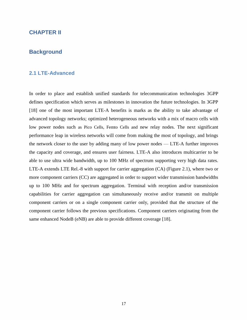
Figure 2. 2: E-UTRAN Overall architecture [4]. ........................................................................................ 20

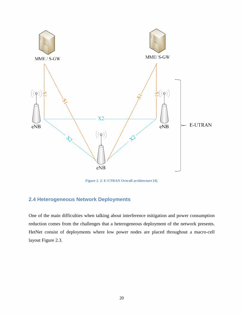
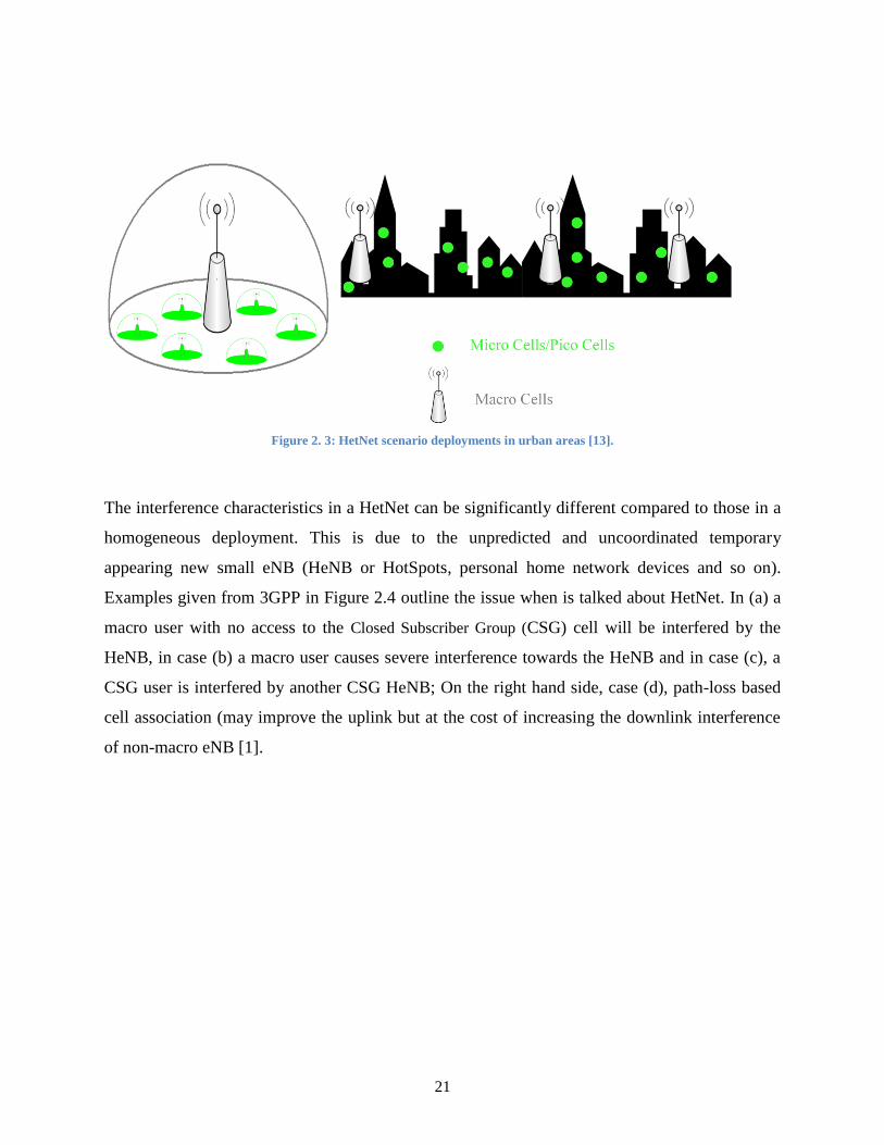
Figure 2. 3: HetNet scenario deployments in urban areas [13]. .................................................................. 21

Figure 2. 4: Examples of interference scenarios in heterogeneous deployment [1].................................... 22

Figure 2. 5: Illustrations of inter-cell interference: downlink phase (left) and uplink phase (right), where

the solid arrow denotes the transmission of useful signal and the dashed arrow denotes the inter-cell

interference [20]. ......................................................................................................................................... 23

Figure 3. 1: Block Scheme of Algorithm for Cell Load Balancing with Energy Consumption

Optimization. .............................................................................................................................................. 28

Figure 3. 2: Main layout of the network with 19 sites; 57 MBSs [14]. ...................................................... 32

Figure 3. 3: Graphical representation of θ and φ [14]. ................................................................................ 33

Figure 3. 4: Vertical Antenna Pattern of a MBS and the antenna mast (left) and Horizontal Antenna

Pattern of 7 sites with 3 MBS each (right) [14]. ......................................................................................... 34

Figure 4. 1: Power Saving Efficiency [%] as a function of used PRB from PBS and distance [m] of the

UE from the MBS. ...................................................................................................................................... 40

Figure 4. 2: The Energy Saving Reliability coefficient in function of 0-20% MBS load and the number of

the PRBs offloaded from the PBS............................................................................................................... 41

Figure 4. 3: The Energy Saving Reliability coefficient in function of 35% MBS load and the number of

the PRBs offloaded from the PBS............................................................................................................... 42

Figure 4. 4: The Energy Saving Reliability coefficient in function of 50% MBS load and the number of

the PRBs offloaded from the PBS............................................................................................................... 42

Figure 4.5: The Energy Saving Reliability coefficient in function of 80% MBS load and the number of the

PRBs offloaded from the PBS. ................................................................................................................... 43

Figure 4.6: The Energy Saving Reliability coefficient in function of 95% MBS load and the number of the

PRBs offloaded from the PBS. ................................................................................................................... 44

Figure 4.7: Overview of the ESR coefficient for the maximum offloading distance according different

MBS loads ................................................................................................................................................... 44

Figure 4.8: ESR at 5% PRB usage recovery between PBS and MBS. ....................................................... 46

Figure 4. 9: ESR at 10% PRB usage recovery between PBS and MBS. ................................................... 46

Figure 4. 10: ESR at 20% PRB usage recovery between PBS and MBS. .................................................. 47

Figure 4. 11: Average additional power per PRB for compensating the interference from MBS. ............. 48

Figure 4. 12: Cumulative Distribution Function per user throughput. ........................................................ 49

Figure 4. 13: Cumulative Distribution Function per cell throughput. ......................................................... 49

7

List of Tables

Table 1. 1: Schematic outline of the thesis ................................................................................................. 16

Table 2. 1: ITU and 3GPP requirements [17] ............................................................................................. 19

Table 3. 1: Network Simulation Parameters ............................................................................................... 34

Table 3. 2: UEs and PBSs deployment restrictions taking into account the network simulator

characteristics [14] ...................................................................................................................................... 36

Table 3. 3: Base Station Power Models Parameters ................................................................................... 37

8

List of Abbreviations

For the purposes of the present document, the abbreviations defined in TR 21.905 [5] and the

following apply. An abbreviation defined in the present document takes precedence over the

definition of the same abbreviation, if any, in TR 21.905 [5].

2G Second Generation

3G Third Generation

3GPP Third Generation Partnership Project

4G Fourth Generation

AWGN Additive White Gaussian Noise

BS Base Station

CA Carrier Aggregation

CC Component Carrier

CDF Cumulative Distribution Function

CSG Closed Subscriber Group

DL Downlink

EDGE Enhanced Data rates for GSM Evolution

eNB enhanced NodeB

EPC Evolved Packet Core

ES Energy Savings

ESE Energy Saving Efficiency

ESM Energy Savings Management

ESR Energy Saving Reliability

9

E-UTRAN Evolved UMTS Terrestrial Radio Access Network

FDD Frequency Division Duplex

GPRS General Packet Radio Service

GSM Global System for Mobile communications

HeNB Home eNB

HetNet Heterogeneous Network

HSPA High Speed Packet Access

ICI Inter Cell Interference

ICIC Inter-cell Interference Coordination

ICT Information and Communications Technology

IMT International Mobile Telecommunications

ITU International Telecommunication Union

LB Load Balancing

LOS Line of Sight

LTE Long Term Evolution

LTE-A LTE–Advanced

MAC Medium Access Control

MBS Macro Base Station

Mcells Macro Cells

MIMO Multiple Input Multiple Output

MME Mobility Management Entity

NLOS Non-LOS

OAM Operations, Administration, Maintenance

OPEX Operating Expenses

10

PBS Pico Base Station

Pcells Pico/Femto Cells

PDCP Packet Data Convergence Protocol

PHY Physical layer

PL PathLoss

PRB Physical Resource Block

QoS Quality of Service

RAN Radio Access Network

RLC Radio Link Control

RN Relay Nodes

RRC Radio Resource Control

RRM Radio Resource Management

S-GW Serving Gateway

SINR Signal Interference to Noise Ratio

SNR Signal to Noise Ration

TRX Transceiver

Tx Transmission

UE User Equipment

UL Uplink

UMTS Universal Mobile Telecommunications System

11

CHAPTER I

Introduction

Technological improvement and fast developments in the wireless communications have been

significant during the recent decade. Increased demands of mobile broadband services were

mainly driven by the successful deployment of Global System for Mobile communications

(GSM) networks. The extension of GSM to General Packet Radio Service (GPRS) including

packet transmission capabilities in the radio interface was a first milestone (commonly named

2.5G) in the evolution path from Second Generation (2G) cellular systems towards the Third

Generation (3G), with Universal Mobile Telecommunications System (UMTS) being one of its

most significant representatives between UMTS and GSM/GPRS technologies. As a result,

wireless technologies are rapidly evolving in order to allow operators to deliver more advanced

multimedia and data transfer services so in this sense, GPRS evolved towards Enhanced Data

rates for GSM Evolution (EDGE) providing higher bit rates comparable to those of UMTS. As

for UMTS, High Speed Packet Access (HSPA) for uplink and downlink is seen as intermediate

evolutionary step since the first wave of UMTS networks rollout, while Evolved UMTS

Terrestrial Radio Access Network (E-UTRAN) is the long term perspective for the Third

Generation Partnership Project (3GPP) technology family [15].

The Fourth Generation (4G) systems are expected to have peak rates of 100 Mbit/s for high

mobility and 1 Gbit/s for low mobility with a good QoS. The macro cells (Mcells), already

deployed by the operator in the network, do not allow the achievement of such high data rates.

This makes it necessary the deployment of pico/femto cells (Pcells). The uncoordinated nature of

the deployment of this smaller cells and the limited amount of electromagnetic spectrum bands

identified as suitable for International Mobile Telecommunications (IMT) leads to high

interference among cells [14].

The driving force to further develop Long Term Evolution (LTE) towards LTE–Advanced (LTE-

A) [17], LTE R-10 from the 3GPP specifications is to provide higher bitrates in a cost efficient

way, and at the same time completely fulfill the requirements set by International

12

Telecommunication Union (ITU) for IMT Advanced, also referred to as 4G. In LTE-Advanced

focus is moved on higher capacity where increased peak data rates.

Next generation wireless HetNet [16] are significant technical challenges that require

advancements in wireless networks architecture, protocol, and management algorithms in order

to build reliable and QoS proved telecommunication infrastructure. There are many networking

protocols at different layers to guarantee and provide integration of the heterogeneous wireless

networks. In addition, managing radio resources among multiple heterogeneous wireless systems

is important to preserve system robustness and QoS. How to fairly and efficiently share radio

resources among multiple networks is one of the major challenges in integrating multiple

networks together.

1.1 Motivation & Goals

A lot of studies based on wireless technology usage indicate that more and more increasing

demand on voice calls, and data traffic is expected and most of it will originated indoors. This

also suggests that a bigger percentage of data traffic and voice calls are made in HotSpot (WiFi)

zones that in fact are business buildings during the day and inhabited buildings during the night

time. This traffic demand, most times follows a predictable pattern where there are peaks and

downs during the day time, depending on the hour.

Today networks have become more complicated with combining different communication

technologies and implementing many new ones in order to meet the market needs. The problem -

how to improve the power efficiency and power saving becomes a significant task in such a

complicated scenario of HetNet. In the telecoms, most mobile network operators aim at reducing

the power consumption without too much influent on their network and the QoS they support to

their subscribers. In such a case, the greenhouse emissions are reduced, while the Operating

Expenses (OPEX) of operators is saved the power efficiency in the infrastructure and terminal

becomes an essential part of the cost-related requirements in network, and there is a strong need

to investigate possible network energy saving solutions [8].

The research community is motivated to innovate a worthy method for improving the network

coverage indoor and in high urban areas. Pico Base Stations (PBS) also called Home eNB

13

(HeNB) appeared to be proper technology solution which to provide this type of improvement,

with their low-power consumption, low-cost and user-oriented deployment. However, the need

to obtain the shared spectrum between Macro Base Stations (MBS) and PBS creates significant

problems of coexistence between the two technologies, as the signal of one is the noise of the

other. Thus it is important to evaluate the risks associated with the deployment of PBSs and how

to decrease them, and thus to prevent capabilities reduction and network malfunction.

1.2 Objectives and Scope

The objectives of this work are:

• Design a power consumption aware metrics for implementation in an algorithm for cell load

distribution that balances the users among Base Stations (BS) in a heterogeneous scenario,

provides fairness to all users and also considers a minimum energy use. This is very important

for successful deployments.

• Study the cell load balancing techniques and algorithm in the current standards to obtain a

reference performance and analysis framework in terms of energy consumption efficiency.

• To identify potential solutions and approaches for energy saving in E-UTRAN in order to meet

LTE, LTE-A performance expectations and current specifications.

• To perform evaluation and implementation of the proposed scenarios, so that they will serve as

a basis for further investigation and simulations of the network performance and energy saving

solutions.

The following use cases will be considered in this study item as defined in [2]:

• Intra-Cell and Inter-Cell Interference consideration in energy saving approaches.

The energy saving solutions identified in this study need to be justified by valid scenario(s), and

based on cell/network load and load balancing situation. The impacts on the existing network

coverage and newly deployed MBS/PBS when introducing an energy saving solution should also

be considered.

The research scope is defined as follows:

14

• User Equipment (UE) accessibility should be guaranteed when a cell is transferred to energy

saving mode.

•QoS should remain in proper levels as well as the other network performance factors like Signal

Interference to Noise Ratio (SINR), Signal to Noise Ration (SNR) .

• Establish a traffic balancing aware scheme in order to fairy allocate the spectrum resources

between the UE(s) during energy saving mode.

• The solutions should not impact negatively the UE power consumption.

1.3 Research Scenario

The research scenario is presented in Figure 1.1. The main idea is to compare the energy

consumption of a PBS to maintain a defined average number of PRBs, then it is assumed that

these PRBs could be offloaded to a BS which is able to serve them(in our case MBS).

A saving power consumption model is defined (Chapter 3.3) and evaluated, at the end the

difference between the saved power from the turned off hardware components in the PBS and

the compensation energy from the MBS to cover the UEs at the referred distance is compared.

Firstly, we accept that there are equally shared physical resources between PBS and MBS, thus

no Intra cell interference exists. In this scenario the load on the MBS and the distance appear to

determine the dimensions of the Energy Saving Reliability ESR and Energy Saving Efficiency

ESE.

Secondly, a scenario is considered, which assumes same PRB usage from both PBS and MBS

which leads to increased interference within the cell coverage area. Here, it is interesting to note

that only small sized remote areas have probability of performing a reliable ESM action.

15

Figure 1. 1: Research scenario of the proposed algorithm

1.4 Research contribution

This study represents the importance of the energy consumption optimization of the

overall network performance. An emphasis is put on reducing the energy consumed by

the network equipment and in particular the small Pico cells.

The approach used concerns methods for establishing a ‗sleep mode‘ state for the small

cells, in which some parts of the hardware could be turned off as long as no active users

are attached to the base station.

The overall proposed solution focused on keeping the QoS at recommended levels thus

providing the users with good enough ‗user experience‘.

A new metrics for estimation and performing ESM decisions are proposed and evaluated.

An algorithm for calculation the stated ESE and ESR coefficients, according to the target

QoS and power consumption efficiency awareness is evaluated.

Analyses of the gained results and basics for future works are given as well.

16

In the current chapter the scope and goals of the thesis presented are given. A schematic

overview of the thesis is represented in Table 1.1 to illustrate the main outline of the presented

work.

Table 1. 1: Schematic outline of the thesis

Chapter II presents an overall view of the state of the art in energy saving scenarios as well as the

interference analysis and interference mitigation. This chapter also focuses on the background

information about LTE/LTE-A and current green communication solutions and the main metrics

used to assess the power efficiency.

Chapter III presents the algorithms used for Energy Saving Management (ESM), as a

representation of the algorithm ESE and ESR are introduced. Approaches for mitigation of the

interference and maintaining the QoS are implemented in our algorithm which is later evaluated

and analyzed.

In Chapter IV, relations among the different scenarios presented in the work are discussed.

Uncoordinated scenario in HetNet where no physical interface between cells exists is considered.

User driven approach - focused on the cell and users throughput. Also the results obtained from

the evaluation are discussed in this chapter, as well as the ESR and ESE.

Finally, in Chapter V the conclusions from this thesis work are presented and future perspectives

are discussed.

•IntroductionChapter 1

•BackgroundChapter 2

•Technical ApproachChapter 3

•Results and Discussion Chapter 4

•Conclusions and Future WorkChapter 5

17

CHAPTER II

Background

2.1 LTE-Advanced

In order to place and establish unified standards for telecommunication technologies 3GPP

defines specification which serves as milestones in innovation the future technologies. In 3GPP

[18] one of the most important LTE-A benefits is marks as the ability to take advantage of

advanced topology networks; optimized heterogeneous networks with a mix of macro cells with

low power nodes such as Pico Cells, Femto Cells and new relay nodes. The next significant

performance leap in wireless networks will come from making the most of topology, and brings

the network closer to the user by adding many of low power nodes — LTE-A further improves

the capacity and coverage, and ensures user fairness. LTE-A also introduces multicarrier to be

able to use ultra wide bandwidth, up to 100 MHz of spectrum supporting very high data rates.

LTE-A extends LTE Rel.-8 with support for carrier aggregation (CA) (Figure 2.1), where two or

more component carriers (CC) are aggregated in order to support wider transmission bandwidths

up to 100 MHz and for spectrum aggregation. Terminal with reception and/or transmission

capabilities for carrier aggregation can simultaneously receive and/or transmit on multiple

component carriers or on a single component carrier only, provided that the structure of the

component carrier follows the previous specifications. Component carriers originating from the

same enhanced NodeB (eNB) are able to provide different coverage [18].

18

Figure 2. 1: Carrier Aggregation – Frequency Division Duplex (FDD). The R10 UE can be allocated resources Downlink

(DL) and Uplink (UL) on up to five Component Carriers. The R8/R9 UEs can be allocated resources on any ONE of the

CCs. The CCs can be of different bandwidths [17].

The driving force to further develop LTE towards LTE–A, LTE R-10 is to provide higher

bitrates in a cost efficient way, and at the same time completely fulfill the requirements set by

ITU for IMT Advanced, also referred to as 4G. In LTE-A focus is on higher capacity- increased

peak data rate, DL 3 Gbps, UL 1.5 Gbps - higher spectral efficiency, from a maximum of

16bps/Hz in R8 to 30 bps/Hz in R10 - increased number of simultaneously active subscribers and

improved performance at cell edges, e.g. for DL 2x2 Multiple Input Multiple Output (MIMO) at

least 2.40 bps/Hz/cell. Each aggregated carrier is referred to as a component carrier. The

component carrier can have a bandwidth of 1.4, 3, 5, 10, 15 or 20 MHz and a maximum of five

component carriers can be aggregated. Hence the maximum bandwidth is 100 MHz. As an

outline the main new functionalities introduced in LTE-A are the enhanced use of multi-antenna

techniques, CA, and support for Relay Nodes (RN) [17].

19

Table 2. 1: ITU and 3GPP requirements [17]

Quantity IMT-Advanced LTE-Advanced

Peak data rate Downlink (DL) 1 Gbit/s

Uplink (UL) 500 Mbit/s

Spectrum allocation Up to 40 MHz Up to 100 MHz

Latency User plane 10 ms 10 ms

Control plane 100 ms 50 ms

Spectrum

efficiency

(4 ant BS,

2 ant terminal)

Peak 15 bit/s/Hz DL 30 bit/s/Hz DL

6.75 bit/s/Hz UL 15 bit/s/Hz UL

Average 2.2 bit/s/Hz DL 2.6 bit/s/Hz DL

1.4 bit/s/Hz UL 2.0 bit/s/Hz UL

Cell-edge 0.06 bit/s/Hz DL 0.09 bit/s/Hz DL

0.03 bit/s/Hz UL 0.07 bit/s/Hz UL

2.1.1 Cells Deployment and Communication Interfaces

The E-UTRAN [4] consists of Macro, Micro, Pico and Fempto cell commonly called eNBs,

providing the E-UTRA user plane (Packet Data Convergence Protocol (PDCP)/Radio Link Control

(RLC)/Medium Access Control (MAC)/Physical layer (PHY)) and control plane Radio Resource

Control (RRC) protocol terminations towards the UE. The eNBs are interconnected with each

other by means of the X2 interface. The eNBs are also connected by means of the S1 interface to

the Evolved Packet Core (EPC), more specifically to the Mobility Management Entity (MME)

by means of the S1-MME and to the Serving Gateway (S-GW) by means of the S1-U. The S1

interface supports a many-to-many relation between MMEs / S-GWs and eNBs. The E-UTRAN

architecture is illustrated in Figure 2.2 below.

20

Figure 2. 2: E-UTRAN Overall architecture [4].

2.4 Heterogeneous Network Deployments

One of the main difficulties when talking about interference mitigation and power consumption

reduction comes from the challenges that a heterogeneous deployment of the network presents.

HetNet consist of deployments where low power nodes are placed throughout a macro-cell

layout Figure 2.3.

21

Figure 2. 3: HetNet scenario deployments in urban areas [13].

The interference characteristics in a HetNet can be significantly different compared to those in a

homogeneous deployment. This is due to the unpredicted and uncoordinated temporary

appearing new small eNB (HeNB or HotSpots, personal home network devices and so on).

Examples given from 3GPP in Figure 2.4 outline the issue when is talked about HetNet. In (a) a

macro user with no access to the Closed Subscriber Group (CSG) cell will be interfered by the

HeNB, in case (b) a macro user causes severe interference towards the HeNB and in case (c), a

CSG user is interfered by another CSG HeNB; On the right hand side, case (d), path-loss based

cell association (may improve the uplink but at the cost of increasing the downlink interference

of non-macro eNB [1].

22

Figure 2. 4: Examples of interference scenarios in heterogeneous deployment [1].

As stated in [1] such scenarios, methods for handling the UL and DL interference towards data

as well as the control signaling, reference signals and synchronization signals are of importance.

Such methods may operate in time, frequency and/or spatial domains. Methods like usage of

different carrier frequencies for different cell layers, or, by restricting the transmission power

during part of the time for at least one cell layer to reduce interference to control signaling on

other cell layers or through different power control schemes as discussed in 3GPP

recommendations.

23

2.5 Interference among cells

Figure 2. 5: Illustrations of inter-cell interference: downlink phase (left) and uplink phase (right), where the solid arrow

denotes the transmission of useful signal and the dashed arrow denotes the inter-cell interference [20].

When we overview both uplink and downlink, transmissions in one cell would interfere the

transmissions in the other neighbor cells if they are operating with the same physical resource. As

shown in Figure 2.5 the downlink, the UE on the cell board is interfered by the signals from other

cells so that it could not successfully recover the signal for its associated eNB. In the uplink, the eNB

is interfered by the signals from other cells so that it could not successfully recover the signal

transmitted by the UE [20]. Thus two main scenarios can be separated and they will be evaluated in

this work in other to gain more realistic results.

2.6 Load Balancing and Inter-cell interference coordination

As defined in [4], Load Balancing (LB) has the task to handle uneven distribution of the traffic

load over multiple cells. The aim is distribution in such a way that radio resources remain highly

utilized and the QoS of in progress sessions are maintained to the extent possible and call

dropping probabilities are kept sufficiently small. LB algorithms may result in hand-over or cell

reselection decisions with the purpose of redistribute traffic from highly loaded cells to

24

underutilized cells. LB is located in the eNB in order to meet the uncoordinated scenario

requirements when the eNB takes Self Organizing Network performance decisions.

Inter-cell Interference Coordination (ICIC) has the task to manage radio resources blocks in way

that ICIC is kept under control. ICIC is inherently a multi-cell Radio Resource Management

(RRM) function that needs to take into account information like the resource usage status and

traffic load situation from multiple cells. The proper ICIC method for a certain deployment may

differ in the UL link and DL link [4].

2.7 Energy Savings and Management (ESM) concept

ESM addresses both Macro and Pico (HeNBs) power consumption and efficiency. Two energy

saving states can be conceptually identified for a network element. The first can be defined as

―notParticipatingInEnergySaving” where no energy saving functions runs and other is

“energySaving‖ - state in which the network element is powered off or restricted in physical

resource usage in different ways. When concerning ―Power Off ―- the radio part of the network

equipment is OFF but the Control part is ON. The radio part of the hardware can be turned ON if

needed if the network performance requires it in order to meet the demands. Based on that

energy saving states, a full energy saving solution includes two elementary procedures:

Energy saving activation: The procedure to switch off PBS/eNB in order to satisfy

energy saving purpose. As a result, a specific network element enters in the energy saving

mode.

Energy saving deactivation: The procedure to switch on PBS/eNB or resume the usage of

corresponding physical resources in order to satisfy the increasing traffic throughput,

QoS or SINR requests. As a result, a specific network element proceeds from

energySaving to notParticipatingInEnergySaving state.

For some use cases of energy saving management, a network element may additionally transition

into the compensatingForEnergySaving state, in which the network element is remaining

powered on, and taking over the coverage areas of geographically closed network element in

energySaving state. The Configuration Management is based on traffic load measurements and

service usage data, Operations, Administration, Maintenance (OAM) can take appropriate

25

actions on the network equipment for improving the energy savings. Examples of such actions

include switch cell or carriers OFF / ON; Reduce or Increase Transceiver (TRX) power [2].

For each of the attempted actions, the potential impact on the network performance like

coverage, capacity or service quality should be assessed and estimated. Clear example is

switching off a cell, which should be performed after the neighbor cells are able to cover the pre-

defined level of capacity, e.g., to estimate the spectrum condition. On the other hand we aim at

high energy efficiency of the performed action, thus, a special purpose coefficient is introduced

in this thesis: Chapter III – 3.1.3 & 3.1.4. Furthermore, before running ESM actions, OAM is

able to compare current traffic load with measurement data obtained from previous days at same

period of time to add even more accurate decision.

2.8 Green Energy

A essential driver of the whole carbon footprint of mobile communications is the number of

worldwide mobile subscriptions. According to statistical researches, the number of mobile

subscribers worldwide increased with a compound annual growth rate of 24%, from around 500

million to over 4 billion between 2000 and 2009 [22]. There were supposed to be about 1.4

billion and over 2 billion regular 3G+ (broadband for phones/smartphones) subscriptions in 2012

and 2014, respectively. The overall number of subscriptions is predicted to increase to about 6

billion in 2014 and tends to reach global penetration of 100% after 2020. Penetration of 100%

means that the number of subscriptions matches the number of dwellers. If only the relevant age

group between 10 and 65 is taken into account, a quasi-100% penetration can be expected

already during 2012 [12].

The other essential driver behind the energy consumption footprint of the mobile

communications is the traffic volume. With the distribution of smartphones and cellular data

subscriptions for laptops, mobile data - traffic shows a rapid rising pattern. The most

weighty type of application is video streaming: it makes highest data volumes, and user

experience is already very good (as it is improving continuously) with modern user

devices and modern networking technology. Notice how mobile data will dominate all mobile

26

traffic (the share of voice is declining); also, mobile data is intended to account for 11-17%

of all Internet Protocol (IP) traffic in 2020. As regards per user statistics, an average mobile

subscription (in all technologies) is supposed to correspond to 8 GB of traffic per year in 2014,

and it will achieve 65 to 100 GB in 2020 [22].

2.9 Telecommunications influence of the CO2

The ever-raising demand for wireless services and ubiquitous network access, however, comes at

the value of a rising carbon footprint for the mobile communications industry. The entire ICT

sector has been evaluated to represent about 2% of global CO2 emissions and about 1.3% of

global CO2 equivalent emissions in 2007 [24]. This study evaluates the relevant figure for

mobile networks to be 0.2% and 0.4% of the global CO2 equivalent emissions in 2007 and 2020,

accordingly. It is significant to notice that these figures include emissions from the entire life

cycle, not only emissions relevant to the operation of mobile networks.

In addition to minimizing the whole footprint of mobile communications, there is a strong

economic drive to decline the energy consumption of these networks. Mobile data traffic is going

to growth rapidly over the next five years, essentially due to a rapid raising in mobile video

traffic, e.g., live video broadcasting and streaming. When considering a increasing whole energy

consumption of the networks driven by the computational complication of modern transmission

methods and raising number of base station sites necessary for high data rates in demand on the

one hand, and constantly growing energy prices on the other, it becomes apparent that energy

consumption is crucial for OPEX of mobile telecom providers.

27

CHAPTER III

Technical Approach

This Chapter presents the algorithms used for ESM. As a representation of the algorithm ESE

and ESR coefficients are introduced and explained. Approaches for mitigation of the interference

and maintaining the QoS are implemented in our algorithm which is later evaluated and

analyzed.

3.1 Algorithm Evaluation

The block scheme of the algorithm - Figure 3.1 represents the overall energy optimization

solution we present in the thesis. A step by step description of the algorithm follows regarding

the consideration and references stated above are taken into account.

In general we distinguish two scenarios with a difference in the Inter Cell and Intra Cell

Interference influence. We suggest an algorithm which efficiently to act in Cell Load Balancing

schemes in order to optimize energy consumption in overall HetNet deployment. A detailed

description of the approach is represented below (Figure 3.1):

28

Figure 3. 1: Block Scheme of Algorithm for Cell Load Balancing with Energy Consumption Optimization.

Block 1 - Used PRBs by PBS: calculates the number of PRBs at given number of users and QoS;

Block 2 - PBS: input data by which is estimated the power per 1 PRB for Pico cell;

SINR - calculated regarding the target SNR for a given user and QoS for PBS;

AWGN - Additive White Gaussian Noise, which is 6,3.10-15

; [14]

ICI - Average value of the interference from a neighboring cells 1,25.10-12

; [14]

*Intra Cell Interference – (Used for Scenario II) Average value of interference from the

macro cell when pico cell is located within macro' range; In case they use same PRB an

interference occurs in the cell area and the network performance is reduces.

29

Block 3 - Power Consumption model PBS: refers to PBS power consumption modem - Formula

(3.12);

Block 4 - Number of PRB to be offload from the PBS: This is the load on PBS determined from

the UEs activity status and traffic demand.

Block 5 - Current Power Consumption of the PBS: This block calculates the current power

consumption of a pico cell at a current moment in function of Block 1 and Block 2;

Block 6 - MBS network performance metrics:

SINR - target SNR for a given user and QoS for macro cell;

AWGN - Additive White Gaussian Noise

Average ICI - Average value of the interference from neighboring cells;

Block 7 – Estimation of the Compensation Power Consumption by MBS: Knowing the number

of the PRBs that have to be offloaded and regarding the energy consumptions parameters for

saving and compensation, the Energy Saving Reliability (ESR) coefficient is determined.

Block 8 - QoS: Determines the overall network and user performance requirements.

Block 9 - Energy Saving Management Decision: Depending on the QoS requirements and the

values of the Energy Saving Reliability and Efficiency is decided whether to transfer PRBs from

Pico cells. It takes into account the free power of Macro cell and free resources.

Block 10 - Calculating the Energy Saving Efficiency coefficient: Determine the percentage of

the saved power if an offload from PBS to MBS is performed.

3.1.1 Scenario I - Fairly Shared PRBs with Inter Cell Interference.

In first scenario only ICI is considered which mitigates the scenario. In addition the resources are

equally shared between the MBS and PBS with no common PRB usage between them, thus no

Intra Cell Interference is taken into account. This allows better performance and results when

30

energy optimization management decisions are taken. The values for AWGN and ICI are

calculated regarding the basic results from simulated network in [14]. This is due to improve the

simulation performance and extend the possibilities of the suggested scenarios for cell load

balancing algorithms with energy consumption awareness.

3.1.2 Scenario II – Uncoordinated Shared PRBs with Intra Cell Interference

In second scenario additional Intra Cell Interference is considered to influence the network

performance. This appears due to the simultaneously usage of a same PRBs from the both MBS

and PBS. A evaluations with 5, 10, 20 and 35 interfered PRBs on PBS are explained detailed (in

Chapter 4.2). This lead to attempt from both the BS to compensate the interference by emitting

more power for PRB to maintain the required QoS and a stage in which the network is congested

could occur. In our case evaluation of the Energy Efficiency is done by calculation ESR and ESE

coefficients regarding the Intra Cell Interference. Samples with up to 35% of PRB recovery are

taken and we established that there is a range within the MBS coverage area where it is energy

efficiently to offload user from PBS to MBS.

3.2 Introduction to the Simulator

3.2.1 Scenarios

The network scenarios specification and performance discussed and analyzed in the thesis are

chosen to take into 3GPP recommendation for carrier aggregation and power efficiency

management [1][14]. In current scenario Macro Sites has three MBS beams, thus forming 3

Micro Cells, are taken into account. Since the goal of this work is to study the power efficiency

and optimization of the network and in particular the network performance regarding the cells

interference, QoS and traffic throughput. The worst interference level scenario is taken into

account. This study will assess several scenarios, starting with a simpler one and improving the

complexity gradually.

31

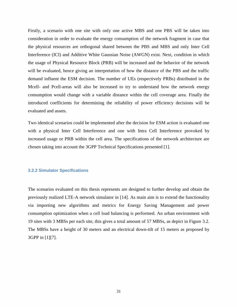
Firstly, a scenario with one site with only one active MBS and one PBS will be taken into

consideration in order to evaluate the energy consumption of the network fragment in case that

the physical resources are orthogonal shared between the PBS and MBS and only Inter Cell

Interference (ICI) and Additive White Gaussian Noise (AWGN) exist. Next, condition in which

the usage of Physical Resource Block (PRB) will be increased and the behavior of the network

will be evaluated, hence giving an interpretation of how the distance of the PBS and the traffic

demand influent the ESM decision. The number of UEs (respectively PRBs) distributed in the

Mcell- and Pcell-areas will also be increased to try to understand how the network energy

consumption would change with a variable distance within the cell coverage area. Finally the

introduced coefficients for determining the reliability of power efficiency decisions will be

evaluated and assets.

Two identical scenarios could be implemented after the decision for ESM action is evaluated one

with a physical Inter Cell Interference and one with Intra Cell Interference provoked by

increased usage or PRB within the cell area. The specifications of the network architecture are

chosen taking into account the 3GPP Technical Specifications presented [1].

3.2.2 Simulator Specifications

The scenarios evaluated on this thesis represents are designed to further develop and obtain the

previously realized LTE-A network simulator in [14]. As main aim is to extend the functionality

via importing new algorithms and metrics for Energy Saving Management and power

consumption optimization when a cell load balancing is performed. An urban environment with

19 sites with 3 MBSs per each site, this gives a total amount of 57 MBSs, as depict in Figure 3.2.

The MBSs have a height of 30 meters and an electrical down-tilt of 15 meters as proposed by

3GPP in [1][7].

32

Figure 3. 2: Main layout of the network with 19 sites; 57 MBSs [14].

The Path Loss (PL) Model in the simulation, regarding by the proposed in 3GPP [1] and further

developed in Matlab environment in [14] which considers different PL for Line of Sight (LOS)

and Non-LOS (NLOS) conditions, where there is no direct channel between transmitter and

receiver. Equations (3.1) and (3.2) gives the PL LOS and the PL NLOS from the Macro base

station to the Users, whereas equations (3.3) and (3.4) express the PLs from the Pico base

stations to the Users.

𝑃𝐿𝐿𝑂𝑆𝑚𝑎𝑐𝑟𝑜 = 103.4 + 24.2 log10(𝑅[𝑘𝑚]) (3.1)

𝑃𝐿𝑁𝐿𝑂𝑆𝑚𝑎𝑐𝑟𝑜 = 131.1 + 42.8 log10(𝑅[𝑘𝑚]) (3.2)

𝑃𝐿𝐿𝑂𝑆𝑝𝑖𝑐𝑜 = 103.8 + 20.9 log10(𝑅[𝑘𝑚]) (3.3)

𝑃𝐿𝑁𝐿𝑂𝑆𝑝𝑖𝑐𝑜 = 145.4 + 37.5 log10(𝑅[𝑘𝑚]) (3.4)

33

Note that R denotes the direct distance between the BS and the UE in km. The MBSs Antennas

Patterns follow the equations (3.7) and (3.8), as proposed by 3GPP [1] and simulated in [14],

what reflects in the vertical and horizontal footprints given by Figure 3.4, respectively. In

equation (3.9) the overall gain is calculated.

𝐺𝑎𝑖𝑛𝑉 = −𝑚𝑖𝑛 12 ∗ 𝜃−𝜀𝑑𝑡𝑖𝑙𝑡

𝜃3𝑑𝐵

2

,𝐺𝑎𝑖𝑛𝑚𝑖𝑛𝜃 (3.7)

𝐺𝑎𝑖𝑛𝐻 = −𝑚𝑖𝑛 12 ∗ 𝜑

𝜑3𝑑𝐵

2

,𝐺𝑎𝑖𝑛𝑚𝑖𝑛𝜑

(3.8)

Where 𝜃 is the vertical angle (Figure 3.3), 𝜀𝑑𝑡𝑖𝑙𝑡 is the electrical down-tilt of the antenna, 𝜃3𝑑𝐵

the value of the 𝜃 at 3dB and 𝐺𝑎𝑖𝑛𝑚𝑖𝑛𝜃 he minim vertical gain. All angles are in degrees.

Figure 3. 3: Graphical representation of θ and φ [14].

𝐺𝑎𝑖𝑛𝑀𝑎𝑐𝑟𝑜 = −𝑚𝑖𝑛 − 𝐺𝑎𝑖𝑛𝑉 + 𝐺𝑎𝑖𝑛𝐻 ,𝐺𝑎𝑖𝑛𝑚𝑖𝑛𝜑

(3.9)

34

Figure 3. 4: Vertical Antenna Pattern of a MBS and the antenna mast (left) and Horizontal Antenna Pattern of 7 sites

with 3 MBS each (right) [14].

3.2.3 Main Parameters of the Simulations

For the referred simulation in matlab[1], the following main parameters are taken into account:

Table 3. 1: Network Simulation Parameters

1. Number of users per Picocell: 10

2. Number of users per Macrocell: 20

3. System Bandwidth: 40MHz

4. Carrier Frequency: 2GHz

5. Number of PRBs per TTI: 200

6. PBSs Tx Power: 36dBm

7. MBSs Tx Power: 49dBm

8. Mcells Operating Mode: FDD

9. Pcells Operating Mode: FDD

10. Transmission Time Interval (TTI): 1ms (> 1ms)

35

3.2.4 Interference

Scenarios in an heterogeneous network appear to be ‗very complicated [14] regarding the

network planning and optimal performance. For this it is important to take in to account the

SINR factor given in equation 3.10:

𝑆𝐼𝑁𝑅𝑐,𝑢𝑛 =

𝑃𝑇𝑋 ,𝑐 ,𝑢𝑛 ∙ ℎ𝑐 ,𝑢

𝑛 2

𝜎2+𝑃𝑝𝑖𝑐𝑜𝑠 ,𝑢𝑛 +𝑃𝑀𝑎𝑐𝑟𝑜𝑠 ,𝑢

𝑛 (3.10)

Where u is the UE, c the Cell and n the PRB, 𝑃𝑇𝑋 the transmission power, |ℎ 2 the channel gain

between the user and the cell and 𝜎2 is the variance of the AWGN. 𝑃𝑝𝑖𝑐𝑜𝑠 , and 𝑃𝑀𝑎𝑐𝑟𝑜𝑠 are the

sum of the powers received by the UE, coming from the Pcells and Mcells, respectively.

Ii is important to note how different deployments of the PBSs inside a Macro Cell area affect the

SINR. If a PBS is next to a MBS it cannot use the same PRBs the MBS is using. This is due to

the fact that the signal of one of the BS would provoke high interference in the others signal,

leading to small SINR and thus preventing the achievement of good data rates. If a PBS is far

from the MBS it can use the same physical channels as the MBS, but it will have to take into

account that high signaling power can increase interference to UEs using that same channels,

even if they are far away. Thus, it is important that the chosen algorithm can act efficiently in

both of these harmful scenarios when the energy consumption is reduced and fairly distributer

resources are available for the users. If two cells are close enough and both need to use the same

PRB they have to use a lower power in order not to kill the communications of the other cell but

still enough to maintain a higher SINR levels. If this is not avoided a low SINR makes the BSs to

start increasing the transmission power, the network enters a stage where no is able to maintain

the required QoS and communicate due to the amount of interference in all PRBs. This also lead

to increased energy consumption and.

36

3.2.5 Traffic Model

The traffic model used in the simulation is the Full-Buffer in order to offer a worst interference

scenario as it considers that the UEs and the Base Stations always contain some information in

the buffer that needs to be sent. The simulation is focused in the DL connection because it is with

higher demands and larger data rates, which makes it more sensitive to the SINR levels. The

number of UEs to be deployed is be determined by the available PRBs.

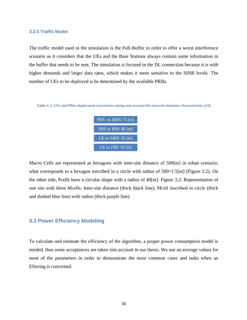
Table 3. 2: UEs and PBSs deployment restrictions taking into account the network simulator characteristics [14]

Macro Cells are represented as hexagons with inter-site distance of 500[m] in urban scenario,

what corresponds to a hexagon inscribed in a circle with radius of 500=1:5[m] (Figure 3.2). On

the other side, Pcells have a circular shape with a radius of 40[m]. Figure 3.2: Representation of

one site with three Mcells: Inter-site distance (thick black line); Mcell inscribed in circle (thick

and dashed blue line) with radius (thick purple line)

3.3 Power Efficiency Modeling

To calculate and estimate the efficiency of the algorithm, a proper power consumption model is

needed, thus some acceptances are taken into account in our thesis. We use an average values for

most of the parameters in order to demonstrate the most common cases and tasks when an

ESaving is concerned.

PBS to MBS 75 [m]

PBS to PBS 40 [m]

UE to MBS 35 [m]

UE to PBS 10 [m]

37

3.3.1 Base Station Power Models

To assess the energy efficiency and in order to take a proper ESM decision, the network energy

consumption of each BS (eNB) has to be estimated and evaluated [3]. Therefore, power models

are needed, that characterize MBS and PBS individually. Since small cells are utilized to cover

only small areas with radios, their transmit power is only a fraction of the MBS‘. Appropriate

power models are used in [3], and in a same manner they will be used in the following analyses.

They can be described by equations 3.11 and 3.12:

𝑃𝑚𝑎 n = 3 𝑁𝑎𝑛𝑡 (n 𝑎𝑚𝑎 𝑃𝑡𝑥 ,𝑚𝑎 + 𝑏𝑚𝑎 ) (3.11)

𝑃𝑝𝑖 n = n 𝑎𝑚𝑖 𝑃𝑡𝑥 ,𝑝𝑖 + 𝑏𝑚𝑖 + n 𝑐𝑝𝑖 (3.12)

Table 3. 3: Base Station Power Models Parameters

Macro Site Pico Site

𝑎𝑚𝑎 3.77 𝑎𝑝𝑖 1.11

𝑏𝑚𝑎 68.73 W 𝑏𝑝𝑖 26.59 W

𝑁𝑎𝑛𝑡 2 𝑐pi 15.26 W

𝑃𝑡𝑥 ,𝑚𝑎 20 W or variable 𝑃𝑡𝑥 ,pi (PRB) 2-4 W

The variables𝑁𝑎𝑛𝑡 , 𝑃𝑡𝑥 ,𝑚𝑎 and 𝑃𝑡𝑥 ,pi denote the number of transmit antennas of a macro

sector‘s BS and the maximum transmit powers of macro and micro BSs, respectively in order to

unify the network overall simulation. 𝑎𝑚𝑎 models the maximum transmit power dependent

energy consumption of the power amplifier, cooling, feeder losses, and power supply, 𝑏𝑚𝑎

summarizes transmit power independent components such as battery backup, signal processing,

and also parts of the cooling unit. 𝑎pi and 𝑏pi are modeled according to the macro site‘s

parameters, except that cooling is omitted. Furthermore, 𝑐pi models additional components, the

power consumption of which scales with the actual load.

The actual power consumption load η on the PBS in percents is given with

η=𝑛 .𝐶𝑝𝑖

100 [%] (3.13)

38

In the MBS power consumption is linearly dependent on the load determined by the used PRB -

n. Table 3.3 gives a more precise information about that parameters. The total power

consumption of all the BSs within the overall cell area A can then be calculated by:

𝑃(n) = 𝑃𝑚𝑎 (n) + 𝑁𝑝𝑖・𝑃𝑝𝑖 (n) (3.14)

Which could be used to evaluate and calculate the overall network power efficiency performance

in future work.

3.3.2 Distributed energy saving management

For distributed ESM, OAM decides on enabling or disabling Energy Saving Action in the

network. When ESM is enabled, network elements execute the energy saving algorithm in a

distributed manner to determine cells to enter ESaving state, ESCompensate state, or No-ES

state – depending on knowledge of current load information of neighboring base stations and

calculations of the ESR or Energy Saving Efficiency (ESE) coefficient. The distributed approach

will requires neighboring base stations to exchange load information on regular intervals.

Consequently, the energy saving algorithm is performed based on coordination a more local

scope compared to the centralized approach.

In summary, for distributed ESM, OAM enables / disables ESM, but the energy saving algorithm

is executed in a distributed manner by network elements that decide which base station should

enter which state (No-ES, ESaving, ESCompensate) [13].

By leveraging on the presence of sufficient underlay macro cell coverage, the small cell

hardware can be augmented with a low-power ―sniffer‖ capability that allows the detection of an

active call from a UE to the underlay macro cell. By doing so, the small cell can afford to disable

its pilot transmissions and the associated radio processing when no active calls are being made

by the UEs in its coverage area [19].

39

3.3.3 Energy Saving Reliability

For the purposes of our work, model (3.11) for PBS power is used. The reduction of the power

consumption of the transmit power independent components in Energy Saving mode is

considered to be 50% of that in normal operating mode e.g. 0,5bpi . This is an average estimated

percentage which is the approximately describes the model of the PBS put into Sleep Mode.

The compensating power from MBS - 𝑃𝑡𝑥 𝑚𝑎 for a PRB is given by equation (3.15):

𝑃𝑡𝑥 𝑚𝑎 =𝑆𝐼𝑁𝑅(𝜎2+𝐼𝐶𝐼)

|ℎ |2 (3.15)

Where ICI is considered to be with an average value of 1,25.10-12

regarding [14] and |ℎ|2 is the

Chanel Gaing (3.16) :

|ℎ|2 = 10 −𝑃𝐿𝑚𝑎𝑐𝑟𝑜 −20−𝑆𝐹 .(𝐺𝑎𝑖𝑛 𝑚𝑎𝑐𝑟𝑜 )

10 (3.16)

SF denotes the shadowing, modeled as a log-normal distribution with mean 0 dB and standard

deviation 8 dB. Finally an Energy Saving Reliability is possible to be determined by (3.17)

ESR =n.P tx pi + 0,5bpi +η

n.P tx ma (3.17)

3.3.4 Energy Saving Efficiency

In this study a main emphasis fall on the newly introduced Energy Saving Efficiency coefficient,

which gives more understandable, percentage value of the after all performance of the

represented algorithm. It is defined by (3.18):

ESE =n.P tx pi + 0,5bpi +η−n.P tx ma

n.P tx pi + bpi + η .100 [%] (3.18)

The main focus is the correlation between the consumed power for maintaining PRBs from the

PBS and the power needed from MBS to serve this PRBs in case of offloading the PBS.

40

CHAPTER IV

Results and Discussion

In this chapter, the algorithms for the scenarios presented in CHAPTER III are discussed based

on the evaluation tests. A comparison of the algorithms is also given. PBSs and UEs are placed

in a particular, known distance in the cell area. Therefore, if real network architectures must be

evaluated, a further test and improvements of the scenarios are needed.

4.1 Evaluating Energy Saving Efficiency

Figure 4.1 shows the results for the evaluation of the energy saving efficiency in dependence of

the distance of the UE form the MBS. It shows the amount of energy that can be saved by

offloading UEs from a PBS and attaching them to a MBS.

Figure 4. 1: Power Saving Efficiency [%] as a function of used PRB from PBS and distance [m] of the UE from the MBS.

5102035

5065

8095

0

10

20

30

40

50

60

70

35

45

55

65

75

85

95

10

51

15

12

51

35

14

51

55

16

51

75

18

51

95

20

52

15

22

52

35

24

52

55

26

5

27

5

28

5

29

5

30

5

31

5

32

5

nu

mb

er

of

PR

Bs

ES

E [

%]

Distance [m]

41

After estimating the saved energy of the overall network performance changes, our method

established that energy effective actions of switching off network equipment could be performed

in distance up to 305 meters from the MBS when the used physical resources from the PBS are

only 5 PRB.

When higher load is handled from the PBS and 50 PRB are about to be offloaded the distance is

more than half time decreased, beginning from 145m. In terms of a maximum loaded PBS with

usage of 95 of 100 available PRB we have the closest distance of efficiency but regarding that

the compensation energy from the MBS is lower we can reach a maximum percentage of

reliability reaching a peak of 65%.

Figure 4. 2: The Energy Saving Reliability coefficient in function of 0-20% MBS load and the number of the PRBs

offloaded from the PBS.

Regarding the Energy Saving Reliability – Figures - 4.2; 4.3; 4.4; 4.5 and 4.6 which is expressed

in function of load of the MBS that is going to assign the UEs offloaded from the PBS It is

significant to be noted that the main factor is the number of the PRBs that are used by PBS.

1

6

11

16

21

26

31

36

35

45

55

65

75

85

95

10

5

11

5

12

5

13

5

14

5

15

5

16

5

17

5

18

5

19

5

20

5

21

5

22

5

23

5

24

5

25

5

26

5

27

5

28

5

29

5

En

erg

y S

av

ing

Rel

iab

ilit

y E

SR

Distance [m]

MBS Load - 20%

5 PRB 10 PRB

20 PRB 35 PRB

50 PRB 65 PRB

80 PRB 95 PRB

42

Figure 4. 3: The Energy Saving Reliability coefficient in function of 35% MBS load and the number of the PRBs

offloaded from the PBS.

Before reaching 50% (Figure 4.4) load on the MBS a minimal difference in the effective distance

is achieved, but further proceeding in evaluation shows that a distance is sharply decreased

above this threshold. It is the transmitting power limitations of the MBS which decrease the

ability to compensate bigger number of PRBs on longer distance.

Figure 4. 4: The Energy Saving Reliability coefficient in function of 50% MBS load and the number of the PRBs

offloaded from the PBS.

1

6

11

16

21

26

31

36

35

45

55

65

75

85

95

10

5

11

5

12

5

13

5

14

5

15

5

16

5

17

5

18

5

19

5

20

5

21

5

22

5

23

5

24

5

25

5

26

5

27

5

28

5

29

5

En

erg

y S

av

ing

Rel

iab

ilit

y E

SR

Distance [m]

MBS Load - 35%

5 PRB 10 PRB20 PRB 35 PRB50 PRB 65 PRB80 PRB 95 PRB

1

6

11

16

21

26

31

36

35

45

55

65

75

85

95

10

5

11

5

12

5

13

5

14

5

15

5

16

5

17

5

18

5

19

5

20

5

21

5

22

5

23

5

24

5

25

5

26

5

27

5

28

5

29

5

En

erg

y S

av

ing

Rel

iab

ilit

y E

SR

Distance [m]

MBS Load - 50%

5 PRB 10 PRB

20 PRB 35 PRB

50 PRB 65 PRB

80 PRB 95 PRB

43

Figure 4.5: The Energy Saving Reliability coefficient in function of 80% MBS load and the number of the PRBs offloaded

from the PBS.

Because of PtxMBS is limited to cover additional PRB when it is working on high loads itself the

distance is reduced to under 85m for taking additional 65 or more PRB. This literally means that

there is trend of decreasing the probability of reducing energy by compensating it with

offloading UE from PBR to MBS while the distance increases. Regarding the lower number of

PRB we have nearly twice decreased distance but still a high very high percentage of efficiency

up to 125m for 95% load. (Figures 4.5 and 4.6)

1

6

11

16

21

26

31

36

35 45 55 65 75 85 95 105115125135145155165175185195205215225235245255265275285295

En

erg

y S

av

ing

Rel

iab

ilit

y E

SR

Distance [m]

BSC Load - 80%

5 PRB 10 PRB

20 PRB 35 PRB

50 PRB 65 PRB

80 PRB 95 PRB

44

Figure 4.6: The Energy Saving Reliability coefficient in function of 95% MBS load and the number of the PRBs offloaded

from the PBS.

As a conclusion for scenario one, Figure 4.7 represents an overview of the evaluated idea for

ESR. It shows that as much loaded is the MBS as more unreliable is to offload users from PBS,

however we defined a certain distance range and number of PRBs at with this is effective even

when MBS is 95% loaded.

Figure 4.7: Overview of the ESR coefficient for the maximum offloading distance according different MBS loads

1

6

11

16

21

26

31

36

35 45 55 65 75 85 95 105 115 125 135 145 155

En

erg

y S

av

ing

Rel

iab

ilit

y E

SR

Distance [m]

BSC Load - 95%

5 PRB 10 PRB20 PRB 35 PRB50 PRB 65 PRB80 PRB 95 PRB

35455565758595

105115125135145155165175185195205215225235245255265275285295

5 10 20 35 50 65 80 95

Ma

x. O

fflo

ad

ing

Dis

tan

ce [

m]

Number of PRBs

0-20%

35%

50%

65%

80%

95%

MBS Load

[%]

45

The low values for ESR and ESE mean that small cells at the MBS cell edge are important for

reducing the overall performance to mitigate the interference and optimize the power

consumption efficiency.

4.2 Evaluating Energy Saving Efficiency – worst case with interference

On the other hand we have the ESR coefficient which adds value to the utility function in order

to give numerical aspect of the Energy Management Reliability and to ease the implementation

of the coefficient in further real performance analyses.

In a scenario where the Macro and Pico cell use the same physical resources, Pico cell will

provide power that is set aside to compensate the additional interference that occurs in such case.

The value is not constant and could be change and depends on it how many numbers of PRB

could be use. For example if the MBS' compensating power is very high, the number of

eventually offloaded PRB would be reduced.

Knowing the distance between the Macro and Pico cell and the interference which each one UE

receives, Pico cell could calculate ESR and marked a decision whether it is possible to save

energy and offload the UEs. There is an option instead of offloading, Pico cell could coordinate

its work with macro cell and receive information for the used resources from the MBS. In this

way the interference could be additionally reduced.

46

Figure 4.8: ESR at 5% PRB usage recovery between PBS and MBS.

We assume the PBS starts to use physical resources with, same as the MBS does. an Intra Cell

Interference appears and the SINR is decreased. Figure 4.8 represents the lowest interference

scenario when only 5% of PRBs are recovering each other.

Figure 4. 9: ESR at 10% PRB usage recovery between PBS and MBS.

1

2

3

4

5

6

7

8

9

35

45

55

65

75

85

95

10

5

11

5

12

5

13

5

14

5

15

5

16

5

17

5

18

5

19

5

20

5

21

5

22

5

23

5

24

5

25

5

26

5

27

5

28

5

29

5

30

5

31

5

32

5

33

5

Co

efic

ien

t E

SR

Distance [m]

Number of

PRBs

5

10

20

35

50

65

80

95

1

2

3

4

5

6

7

8

9

35

45

55

65

75

85

95

10

5

11

5

12

5

13

5

14

5

15

5

16

5

17

5

18

5

19

5

20

5

21

5

22

5

23

5

24

5

25

5

26

5

27

5

28

5

29

5

30

5

31

5

32

5

33

5

Co

efic

ien

t E

SR

Distance [m]

Number of

PRBs

5

10

20

35

50

65

80

95

47

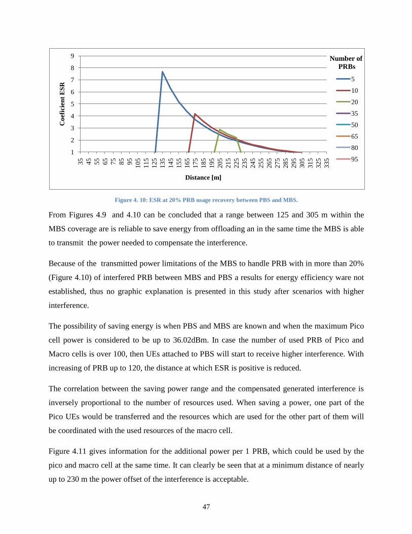
Figure 4. 10: ESR at 20% PRB usage recovery between PBS and MBS.

From Figures 4.9 and 4.10 can be concluded that a range between 125 and 305 m within the

MBS coverage are is reliable to save energy from offloading an in the same time the MBS is able

to transmit the power needed to compensate the interference.

Because of the transmitted power limitations of the MBS to handle PRB with in more than 20%

(Figure 4.10) of interfered PRB between MBS and PBS a results for energy efficiency ware not

established, thus no graphic explanation is presented in this study after scenarios with higher

interference.

The possibility of saving energy is when PBS and MBS are known and when the maximum Pico

cell power is considered to be up to 36.02dBm. In case the number of used PRB of Pico and

Macro cells is over 100, then UEs attached to PBS will start to receive higher interference. With

increasing of PRB up to 120, the distance at which ESR is positive is reduced.

The correlation between the saving power range and the compensated generated interference is

inversely proportional to the number of resources used. When saving a power, one part of the

Pico UEs would be transferred and the resources which are used for the other part of them will

be coordinated with the used resources of the macro cell.

Figure 4.11 gives information for the additional power per 1 PRB, which could be used by the

pico and macro cell at the same time. It can clearly be seen that at a minimum distance of nearly

up to 230 m the power offset of the interference is acceptable.

1

2

3

4

5

6

7

8

9

35

45

55

65

75

85

95

10

5

11

5

12

5

13

5

14

5

15

5

16

5

17

5

18

5

19

5

20

5

21

5

22

5

23

5

24

5

25

5

26

5

27

5

28

5

29

5

30

5

31

5

32

5

33

5

Co

efic

ien

t E

SR

Distance [m]

Number of

PRBs

5

10

20

35

50

65

80

95

48

Figure 4. 11: Average additional power per PRB for compensating the interference from MBS.

Figures 4.12 and Figure 4.13 show the Cumulative Distribution Function (CDF) per user and cell

throughput compared to the distance between the macro and Pico cell. It can clearly be seen that

when the distance decreases, the Pico UEs start to experience higher interference, which reduces

their speed.

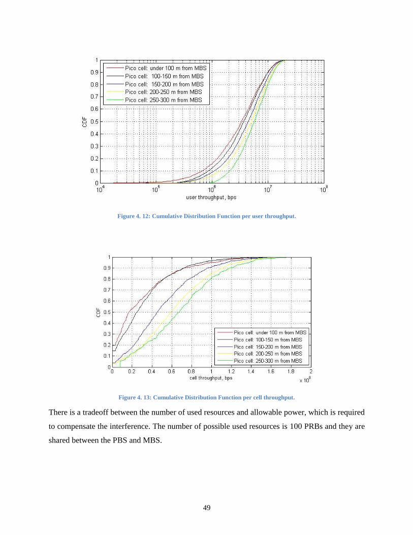
49

Figure 4. 12: Cumulative Distribution Function per user throughput.

Figure 4. 13: Cumulative Distribution Function per cell throughput.

There is a tradeoff between the number of used resources and allowable power, which is required

to compensate the interference. The number of possible used resources is 100 PRBs and they are

shared between the PBS and MBS.

50

51

CHAPTER V

Conclusions and Future Work

This chapter summarizes the main conclusions of this work and presents further practical

considerations along with related future work.

5.1 Conclusions

The main focus of this thesis was Cell Load Balancing in HetNet regarding uncoordinated

deployment of the BS (eNB) and regarding the energy consumption. The approach which is used

in the proposed solution puts an emphasis on the Power Saving Efficiency of the E-UTRAN

LTE-A cellular system, corresponding to the uplink direction of the 3GPP Long Term Evolution

Project.

All the results in Chapter IV where obtained by MATLAB simulations and by averaging the

results and evaluated by the proposed here algorithm. It was shown that the conceptual idea is

sound, however, future work should include testis and evaluations with ―real networks‖ scenario.

Comparing the two scenarios, it was confirmed that more energy could be saved when enabling a

Sleep Mode/Power Saving Mode on low power network equipment, e.g., PBS. The aim of the

project was to obtain a cell load balancing scheme and we came up with the solution for

calculating the efficiency and reliability of taking Energy Saving Management actions, before

offloading a UE form the BSs. This leads to an improved energy awareness of the

telecommunications network because it helps reduce the consumed energy, respectively,

reducing the CO2 emissions.

Firstly, an assessment of the main network performance metrics, which reflects on the QoS and

the traffic throughput, was performed. Then, after an evaluation through the proposed in this

work energy consumption improvement algorithm, a coefficient determining the reliability of

offloading users from BSs regarding the compensating power needed for them to be

compensated from another BS (in our case from PBS to MBS) was introduced.

52

A model for determining the power consumption of a PBS was proposed and applied in order to

calculate the energy consumption for maintaining a defined number of PRB on that PBS.

Another model was proposed and applied for the calculation of the needed compensating power,

from the side of the MBS. A reduction by 50% in the energy consumption in Sleeping mode

(when no active UE attached) was observed.

Finally, the two performances were compared. Based on the obtained results, we established a

model for the reliability of offloading the UEs from one BS to another. Two interference

scenarios were considered: intra-cell and Inter-Cell. It was confirmed that in an Inter Cell

Interference scenario, the closer the PBS is to the MBS, a higher reliability I for turning off the

small network equipment, while still maintaining reasonable QoS can be achieved. For the Intra

Cell Interference case, we have the opposite results concerning the distance from MBS. In such

scenarios, energy optimization should be performed via offloading users located in the more

remote points of the MBS coverage area, but in this case, some restrictions were observed for the

ability of the MBS to handle the interference and thus only a small amount of PRBs (for example

between 175m and 305m for 105 PRB) were actually effective for offloading.

5.2 Future works

Future work envisions tests in real network scenarios and the implementation of an algorithm for

the coordination between the network equipment in order to be able to offload UEs to exact BS

(eNB) where they will have the best performance and QoS level.

The main functionality which could be added to achieve more realistic results is the dynamic

changing of the UE‘s distance from the BS and functionality for calculating the reliability in real

time. This also requires handover functionality and additionally, affects the network productivity.

For the presented algorithm itself, a more realistic model which simultaneously assesses the

reliability of offloading all the users at the same time would be a significant step forward.

As far as the power consumption, is concerned, a statistical background history could be

followed to predict the network behavior and increase the algorithm‘s performance.

53

References

[1] 3GPP TR 36.814 v9.0.0, ―3rd Generation Partnership Project; Technical Specification Group

Radio Access Network; Evolved Universal Terrestrial Radio Access (E-UTRA); Further

advancements for E-UTRA physical layer aspects; (Release 9)‖, March 2010.

[2] 3GPP TR 32.826 v10.0.0, ―Technical Specification Group Services and System Aspects;

Telecommunication management; Study on Energy Savings Management (ESM); (Release 10)‖,

March 2010.

[3] 3GPP TR 32.826 v10.0.0, ―3rd Generation Partnership Project; Technical Specification

Group Services and System Aspects; Telecommunication management; Study on Energy

Savings Management (ESM); (Release 10)‖, March 2010.

[4] 3GPP TS 36.300 v8.3.0, ―3rd Generation Partnership Project; Technical Specification Group

Radio Access Network; Evolved Universal Terrestrial Radio Access (E-UTRA) and Evolved

Universal Terrestrial Radio Access Network (E-UTRAN); Overall description; Stage 2; (Release

8)‖, December 2007.

[5] 3GPP TR 21.905 v10.3.0, ―3rd Generation Partnership Project; Technical Specification

Group Services and System Aspects; Vocabulary for 3GPP Specifications; (Release 10)‖, March

2011.

[6] 3GPP Green activities, ―Energy Saving v0.1.0‖, September 2012.

[7] ETSI TR 136 912 v9.1.0, ―LTE; Feasibility study for Further Advancements for E-UTRA

(LTE-Advanced); (3GPP TR 36.912 version 9.1.0; Release 9)‖, January 2010.

[8] ETSI TR 136 927 v10.1.0, ―LTE; Evolved Universal Terrestrial Radio Access (E-UTRA);

Potential solutions for energy saving for E-UTRAN; (3GPP TR 36.927 version 10.1.0; Release

10)‖, October 2011.

[9] ETSI TS 132 551 v11.3.0, ―Universal Mobile Telecommunications System (UMTS); LTE;

Telecommunication management; Energy Saving Management (ESM); Concepts and

requirements; (3GPP TS 32.551 version 11.3.0; Release 11)‖, February 2013.

54

[10] ETSI TS 136 300 v11.5.0, ―LTE; Evolved Universal Terrestrial Radio Access (E-UTRA)

and Evolved Universal Terrestrial Radio Access Network (E-UTRAN); Overall description;

Stage 2; (3GPP TS 36.300 version 11.5.0; Release 11)‖, April 2013.

[11] ETSI TS 102 706 v1.2.1, ―Environmental Engineering (EE) Measurement Method for

Energy Efficiency of Wireless Access Network Equipment‖, October 2011.

[12] EARTH INFSO-ICT-247733 Deliverable D2.1, ―Economic and Ecological Impact of ICT‖,

April 2011.

[13] QUALCOMM, ―HSPA+ Advanced: Taking HSPA+ to the Next Level‖, 2012.

[14] Nuno Emanuel Cabral Monteiro, ―Interference Analysis in a LTE-A HetNet Scenario:

Coordination vs. Uncoordination‖, June 2012.

[15] Jordi Perez-Romero, Xavier Gelabert and Oriol Sallent, ―Radio Resource Management for

Heterogeneous Wireless Access Networks‖, 2008.

[16] Fei Richard Yu, Helen Tang and Hong Ji, ―Radio Resource Management and Admission

Control in Heterogeneous Wireless Access Networks‖, 2008.

[17] Jeanette Wannstrom, ―LTE-Advanced‖, for 3GPP, May 2012.

[18] Eiko Seidel, ―Progress on ‗LTE Advanced‘ - the new 4G standard‖, July 2008.

[19] Imran Ashraf, Federico Boccardi, Lester Ho, ―Power Savings in Small Cell Deployments

via Sleep Mode Techniques‖, 2010.

[20] Peng Guan, ―Combining relaying and base station coordination for improving cell-edge

multi-user performance in 3GPP LTE-Advanced networks‖, June 2011.

[21] Henrik Klessig, Albrecht J. Fehske, and Gerhard P. Fettweis, ―Energy Efficiency Gains in

Interference-limited Heterogeneous Cellular Mobile Radio Networks with Random Micro Site

Deployment‖, 2011.

[22] International Telecommunication Union, ―Worldwide mobile cellular subscribers to reach 4

billion mark late 2008‖, Press release, 2008.

55

[23] The Climate Group, ―SMART2020: Enabling the low carbon economy in the information

age‖, 2008.

[24] ITU-D, ―Key Global Telecom Indicators for the World Telecommunication Service Sector‖,

2010. http://www.itu.int/ITU-D/ict/statistics/at_glance/KeyTelecom.html