cef.up working paper 2013-09

VOLUME UNCERTAINTY IN CONSTRUCTION PROJECTS: A REAL OPTIONS APPROACH

João Adelino RibeiroPaulo Jorge Pereira

Elísio Brandão

Volume Uncertainty in Construction Projects: a

Real Options Approach

João Adelino Ribeiro∗†, Paulo Jorge Pereira

‡and Elísio Brandão

§

May 27, 2013

Abstract

The levels of uncertainty surrounding construction projects are particularly high and construction managers shouldbe aware that adequately managing the effects of the different types of uncertainty may lead to an increase in theproject’s final Net Present Value (NPV). The model proposed focus on the impact that a specific type of uncertainty -volume uncertainty - may produce in the project’s expected NPV. Volume uncertainty is present in most constructionprojects since managers do not know, during the bid preparation stage, the exact volume of work that will beexecuted during the project’s life cycle. Volume uncertainty leads to profit uncertainty and the model integratesa discrete-time stochastic variable, designated as “additional value”, i.e., the value that does not directly derivefrom the execution of the tasks specified in the bid documents, and which can only be quantified with precisionby undertaking an incremental investment in human capital and technology. The model determines that, even onlyrecurring to the skills of their own experienced staff, contractors will produce a more competitive bid, provided thatthe expected amount for the additional profit is greater than zero. However, construction managers often need tohire specialized firms and highly skilled professionals in order to quantify, with accuracy, the expected amount ofadditional value and, hence, the precise impact of such additional value in the optimal bidding price. Based on theoption to sign the contract and to perform the project by the selected bidder, identified and evaluated by Ribeiro et al.(2013), the model’s outcome is the threshold value for this incremental investment. A decision rule is then reached:construction managers should invest in human capital and technology provided that the cost of such incrementalinvestment does not exceed the predetermined threshold value. The model also proposes new forms of reachingthe optimal bidding price, considering solely the effects of the non-incremental investment and also considering thepossible impact of the incremental investment in human capital and technology.

JEL Classification Codes: G31; D81.

Keywords: real options; construction projects; investment decisions; optimal bidding.

∗PhD Student in Finance, Faculty of Economics, University of Porto, Portugal; email: 090427012@fep.up.pt†João Adelino Ribeiro acknowledges the financial support provided by FCT (Grant nº SFRH/BD/71447/2010)‡Assistant Professor at Faculty of Economics, University of Porto, Portugal; email: pjpereira@fep.up.pt§Full Professor at Faculty of Economics, University of Porto, Portugal; email: ebrandao@fep.up.pt

1

Part I

Introduction

1 Uncertainty in Construction Projects in the Context of Bidding Competitions

Uncertainty surrounding construction projects is a crucial element that should be ade-

quately managed since it may have a huge impact in construction companies overall per-

formance. Construction companies or contractors are firms operating in the construction

industry whose business reside in executing a set of tasks previously established by the

client.1 The amount of tasks to be performed constitutes a project, job or work. The vast

majority of projects in the construction industry are assigned through what is known as

“tender” or “bidding” processes (Christodoulou (2010); Drew et al. (2001)), this being

the most popular form of price determination (Liu and Ling (2005); Li and Love (1999)).

In a tender or bidding process, a certain number of contractors (bidders) compete to ex-

ecute a project by submitting a single-sealed proposal until a specific date previously

defined by the client. Potential bidders have access to a what is commonly known as

the “bid package”. This package contains a set of technical pieces (often also referred

as “tender documents”) which will serve as the basis for determining the price to include

in the bid proposal. More specifically, the package includes plans and technical draw-

ings, a proposal form, the “general conditions” covering procedures which are common

to all construction contracts and the “special conditions” containing the procedures to be

used and that are unique to the project in question (Halpin and Senior (2011)), including

information about the type of contract that will be enforced.

The usual format of a tender or bidding process is based on the rule that - all other things

being equal - the contract will be awarded to the competitor that submitted the lowest

price (Christodoulou (2010); Cheung et al. (2008); Chapman et al. (2000)) or, which is1For the purposes of this research, we exclude those situations where contractors execute their own

projects, as it is often the case of construction companies operating in the real estate sector.

2

the same, the lowest bid. The bidder that proposed the lowest price will most likely be

invited to sign the contract and, if the contract is actually signed, he or she will have to

invest a substantial amount of money by incurring in the necessary direct costs to execute

the project, i.e., the construction costs.

Traditionally, construction management literature has been placing more emphasis on the

negative effects of uncertainty, which means researchers seem to be more concerned with

ways to deal with the risks involving the construction activities and how they may af-

fect the project’s expected Net Present Value (NPV) through a negative impact in the

construction costs. In fact, few authors have been addressing uncertainty as a source of

opportunity, as it is the case of Ford et al. (2002), Ng and Bjornsson (2004) and Yiu

and Tam (2006). Ford et al. (2002) argued that construction projects may include spe-

cific sources of uncertainty that affect project value, but not necessarily just by reducing

it. This argument is supported by Ng and Bjornsson (2004) when they state that, even

though uncertainty can lead to cost over-runs and delays, it can also produce positive re-

turn if managed properly. Following the same line of thought, Yiu and Tam (2006) applied

the real options approach to evaluate the intrinsic value of uncertainty and the managerial

flexibility deriving from the options to defer and to switch modes of construction. There-

fore, uncertainty can also be seen as a source of opportunities, rather than just an element

that may cause undesirable effects during the construction stage - in clear opposition to

the traditional view that ”all uncertainty presumed loss” (Mak and Picken (2000)).

Ford et al. (2002) acknowledge the fact that many construction project conditions evolve

over time and thus managerial choices for effective decision-making cannot be completely

and accurately determined during the pre-project planning period. In fact, these authors

observe that many aspects of construction projects are uncertain, such as input prices, the

weather conditions, the length of some activities and the overall duration of the project,

among others, meaning that the effects of some of these sources of uncertainty can only be

recognized and properly managed as the project unfolds. This argument is also supported

by Mattar and Cheah (2006) when they mention that contractors typically learn more

3

about the value of the project as they invest over time and uncertainties are resolved.

Even though we recognize the fact that the possible consequences of some sources of un-

certainty cannot be anticipated, we do believe that others can be predicted and accounted

for during the bid preparation process. Moreover, we will try to demonstrate that is pos-

sible to establish a support decision model that accommodates the expected impact of a

specific type of uncertainty - the uncertainty associated with the amount of work to be

executed during the project’s life cycle.

This piece of research builds on this crucial aspect by focusing on a specific source of

uncertainty which may lead to a greater NPV by increasing the expected amount of work

to be executed during the construction stage. This means we believe that this source of

uncertainty is - at least - as decisive as the others in adding value to the project. Therefore,

managers should recognize its importance by planning and strategically managing this

element in a way that improves the project’s NPV and, as we will demonstrate, their

competitiveness in a bidding competition context.

Despite the fact that project value can be substantially increased by reducing costs, we

would like to reinforce the idea that project value can also be increased by raising more

income. As we will see, more income means the income that is generated through actu-

ally executing, during the construction phase, a certain amount of tasks which were not

included in the tender documents. We are thus concerned with the uncertainty that may

lead to more project value by increasing the amount of work to be performed by contrac-

tors, “vis-a-vis” with the amount of work contractors are contractually bound to execute.

We will refer to this type of value as “hidden-value”.2

Hidden-value should be captured and quantified in the pre-project stage while the bid pro-

posal is being prepared, by carefully analyzing the portions of the project where it may

be concealed. Ford et al. (2002) observed that hidden-value is present in the most uncer-

tain portions of the project, enabling us to sustain that skilled engineers and experienced

2To the best of our knowledge, this designation was first adopted by Ford et al. (2002) and, in the contextof their research, the definition encompasses other sources of hidden-value, rather than just those which mayresult in additional income.

4

managers - whose responsibility is to prepare the bid proposal - have a fairly good knowl-

edge, based on their accumulated experience, of “where to look for”. Chapman et al.

(2000) stated that the bid preparation process begins with a preliminary assessment of the

tender documents. We sympathize with this statement and argue that, in this preliminary

assessment, is possible to recognize and quantify hidden-value and, more specifically, to

stipulate a high-estimate and a low-estimate to this hidden-value and to attribute a prob-

ability of occurrence to each of the estimates just by undertaking a preliminary analysis

of the tender documents.3 However, the quantification of hidden-value with accuracy is,

in most practical situations, a goal that can only be achieved by performing an exhaustive

investigation of all the bid documents. For this purpose, many construction companies

will have to invest in human capital and technology, which, in some cases, may imply hir-

ing skilled technicians specialized in this type of tasks (Kululanga et al. (2001)), as well

as contracting highly specialized firms possessing the necessary technology to carry out

specific type of works with the purpose of supplying contractors with more accurate infor-

mation concerning the project in hands. Kululanga et al. (2001) clearly support this idea

when they state that an awareness of job factors, which may give rise for claiming extra-

revenues due to extra-work to be executed is a skill that, generally, has to be specially

acquired. Pinnell (1998) reinforces this argument when he mention that the individual (or

the team) responsible for thoroughly analyzing the bid documents aiming to capture and

quantify hidden-value during the bid preparation process may be a consultant expert or

a team of consultant experts. Whether this incremental investment in hiring skilled con-

sultants and contracting highly specialized firms aiming to supply contractors with more

accurate information regarding the volume of work to be performed will be worthwhile

constitutes the question we will address using the model proposed in Part II.

Our model is thus based on the argument that uncertainty can add value to construc-

tion projects through the impact caused in the amount of work to be executed during the

project’s life cycle. This argument entails that contractors do not know, before the com-

3Our model will just contemplate a specific type of hidden-value: the one that may result in the creationof additional profit through the execution of more volume of work.

5

pletion of the project (or, at least, before the job begins), how much volume of work will

effectively be executed. Hence, uncertainty is present concerning the volume of work,

allowing us to designate this construction project-specific type of uncertainty from the

contractor’s perspective as “volume uncertainty”. Volume uncertainty obviously leads to

uncertainty about the project’s final NPV since the execution of additional work implies

receiving extra income (or extra revenues) and incurring in extra costs. We will designate,

from now on, the difference between these extra revenues and these extra costs as “ad-

ditional value”. Additional value is, therefore, the value that may be generated because

there is, at least, a specific source of uncertainty surrounding construction projects that

may actually cause such effect. We now proceed to discuss this subject with more detail.

2 Recognizing and Quantifying Hidden-Value: The Concept of Additional Value

In many construction projects value is hidden in the most uncertain portions of the project,

as we mentioned previously. After its detection and quantification, hidden-value becomes

what we designate as additional value. To fully understand how hidden-value may be

detected and properly quantified - and, hence, transformed into additional value - we

must first know where hidden-value can be detected, which means we have to understand

the nature of its sources.4

The construction management literature has been dedicating strong attention to a sub-

ject commonly known as “Claims”. A construction claim can be defined as “a request

by a contractor for compensation over and above the agreed-upon contract amount for

additional work or damages supposedly resulting from events that were not included in

the initial contract” (Adrian (1993)). This well-known definition implies that contrac-

tors can and should ask for a compensation when they execute works that were not con-

sidered in the initial contract.5 Thomas (2001) argued that variations to the work are

4The pure detection of hidden-value does not necessarily result in the creation of additional value to theproject. The increase in the project’s expected NPV will only occur if the execution of the extra volume ofwork originates a profit. We will discuss this important aspect later.

5This definition also implies that there are other sources which may raise more income.

6

almost inevitable and Dyer and Kagel (1996) went even further when they stated that

- inevitably (sic) - situations arise where clients actually deviate from the original con-

struction scope, which means that, most likely, the initial scope will be increased. These

statements strongly sustain our argument that, at least frequently, contractors do end up

executing more work than the one deriving from what is established in the tender docu-

ments. Consequently, both statements also support the argument that contractors do not

know, ex-ante, the precise amount of work they will be executing throughout the whole

duration of the project.

Rooke et al. (2004) categorize construction claims in two different types: (i) proactive

claims and (ii) reactive claims. Proactive claims are the ones that can be anticipated and,

thus, planned for at the bid preparation stage. On the other hand, reactive claims are the

ones which can only be recognized in the course of the project itself, in response to un-

foreseen events. Even though we are aware that reactive claims may have a considerable

impact in the project’s final NPV, we exclude them from our model precisely because they

are, by definition, unforeseeable, which means that no acceptable estimate can be drawn.

Therefore, our model incorporates estimates for those proactive claims which derive from

the existence of uncertainty regarding the volume of work to be performed.6

2.1 Sources of Additional Value

There are two sources of uncertainty that may result in claims through the execution of

more volume of work than the one directly deriving from the information contained in the

bid package. We classify them as being of two different kinds: (i) extra quantities and (ii)

additional orders.6As we will carefully explain, depending on the contractual arrangements binding the parties, there is a

specific type of volume uncertainty which does not necessarily generate more income.

7

2.1.1 Extra Quantities

Extra quantities occur when the contractor ends up executing, in the field, more quantities

of a specific item than the ones specified in the tender documents. As we will see, if the

type of contract allows such, the contractor will receive the unit price included in his or

her proposal multiplied by the quantities he or she has actually executed and after being

measured in the field by the client or the client’s agent.7 Under such contractual con-

ditions, field quantities are the quantities that matter because they are the ones that will

generate the income associated with the execution of each task included in the bid pack-

age. Ideally, from the client’s point of view, field quantities should match the quantities

included in the tender documents. However, frequently, discrepancies between the quan-

tities estimated by the client and quantities actually executed in the field are observed.

The literature refers that this inaccuracy is mainly due to the poor quality of the tender

documents (see, for example, Laryea (2011); Rooke et al. (2004); Akintoye and Fitzger-

ald (2000)), meaning that the client´s estimates are not always accurate and, therefore,

tender documents provided to the bidders often contain mistakes.

Bearing this in mind, most experienced contractors do not take for granted the accuracy

of the information contained in the tender documents regarding the quantities to be per-

formed when they are preparing the bid. On the contrary, if hidden-value is to be captured

and quantified - since inaccuracies in the tender documents are likely to occur - mis-

takes can only be recognized if a proper measurement of all the technical drawings is

performed. This is an important aspect we must stress: contractors will only know, with a

strong degree of certainty, how many quantities they will be executing during the project’s

life cycle if a thorough and accurate measurement of all the technical drawings included

in the bid package is undertaken. Moreover, as Rooke et al. (2004) stated, pricing a ten-

der involves reading through bills of quantities often several inches thick, meaning that

the quantities stated in the bill must be confronted with the quantities obtained after per-

7Such fact also implies that the contractor will receive less income if the quantities executed in the fieldare smaller than the ones specified in the bid documents.

8

forming a complete examination of all the drawings provided by the client. Rooke et al.

(2004) also argued that most of the times - especially in the case of non-large contractors -

companies do not have experts in this type of highly skilled job or, if they do, the amount

of work in hands in a particular moment may imply the need for hiring external experts.

This aspect is reinforced by the fact that contractors actually express concern over what

they consider to be a short period of time that is normally allowed for bid preparation, as

Laryea and Hughes (2008) observed.

2.1.2 Additional Orders

Additional orders, also known as “change orders”, refer to a task or a set of tasks the

contractor effectively performs during the project’s life cycle, which possess a different

nature from the ones specified in the bid package. This source of uncertainty that may

give rise to additional work and extra profit is, thus, different from the one mentioned be-

fore, since change orders are related with varied work which is not of a similar character,

or is not carried out under similar conditions than the one contained in the bill of quan-

tities (Davinson (2003)).8 However, we need to make clear that these tasks may include,

for the purposes of their completion, the execution of an item or a set of items that ac-

tually were considered in the bill of quantities and previously priced by the bidder, since

they were part of the project’s initial scope. Hence, when contractors look for mistakes

in the tender documents, they do not focus their attention merely in finding discrepancies

that may lead to the execution of extra quantities solely associated with the tasks spec-

ified in the bid package. Instead, experienced engineers and skilled experts also search

for possible tasks, which are likely to be executed and were not specified in the tender

documents. By carefully analyzing all the plans and drawings provided by the client, it

is possible to recognize that some parts of the project (or even the project “seen” as a

whole) will not be properly completed if only the tasks included in the tender documents

8Change orders are also often designated as “increase in scope”. The designation obviously acknowl-edges the fact that the scope of the original project becomes wider, which means the contractor will executea certain number of tasks that were not included in the technical pieces that supported the initial contract.

9

are to be performed. Hence, additional orders can and should be considered as a potential

source of additional value and our model will encompass this argument by assuming that

contractors are able to stipulate a high-value estimate and a low-value estimate for addi-

tional orders, and also attribute, to each of these estimates, a probability of occurrence.

For the purpose of defining the two estimates, we argue that contractors need to take into

account: i) the amount of work the additional orders will generate in comparison to the

amount established in the original contract; ii) the previous experience with the client as

well as their history and frequency of placing new orders; iii) the bargaining skills of the

client throughout the negotiation process.

2.2 Types of Contract

To fully understand the possible impact of the two sources of additional value on the

project’s expected NPV, we have to relate each of them with the type of contract that

will bind the parties. Construction management literature addresses with more relevance

two types of contracts (see, for example, Halpin and Senior (2011); Clough et al. (2000);

Woodward (1997)): (i) the “unit-price” type of contract and (ii) the “lump-sum” type of

contract.9

The unit-price contract allows for flexibility in meeting variations regarding the amount

and quantity of work encountered during the construction stage. This means that, when

this type of contract is adopted, the project is broken down into work items, which are

characterized by units, such as cubic yards, linear and square feet, and piece numbers

(Halpin and Senior (2011)). This fact implies that the contractor, during the bid prepara-

tion stage, will quote the price by units rather than as a single total contract price. Hence,

if for some reason, the contractor effectively executes more quantities of one or more

specific items included in the bill of quantities, he or she will be receiving the amount

that results from multiplying the number of units executed by the unit price he or she has

9Other types of contract are mentioned in the literature, as the “cost-plus-fee” type and the “cost-reimbursement” type. However, unit-price and, especially, lump-sum contracts are the ones that are mostcommonly adopted, particularly in the context of bidding competitions.

10

included in the bid proposal.

If the type of contract enforced is the lump-sum, bidders are asked to price a specific

task or item, regardless of the number of units that will actually be executed. Hence,

if this type of contract is adopted, contractors will never receive more (less) income for

executing more (less) quantities of an item or items clearly specified by the client than

those he or she has predicted after analyzing the drawings and other technical documents

contained in the bid package. The risk associated with the likelihood of performing more

quantities than those that served as the basis for computing the corresponding global price

for a specific task (or a group of tasks) is, thus, borne by the contractor. However, the

contrary can also occur: contractors might actually perform less quantities in the field than

those considered during the tender preparation stage, and which served as the basis for

establishing the proposed price. Hence, and even though this specific type of uncertainty

still exists when the parties are bounded by a lump-sum contract, it is not possible to

account for its effects during the bid preparation stage since the contractor will only be

aware if any additional value is actually raised through this mean after the task or tasks

in question are executed, i.e., as the project unfolds. Therefore, this source of uncertainty

may affect the project’s final NPV but can not be quantified before the work begins. Being

so, in the presence of a lump-sum contract, additional value may only be obtained through

the execution of additional orders whereas, if the contract assumes the unit-price type,

both sources of uncertainty may create additional value by increasing the volume of work

to be performed.10

Lump-sum contracts are the most common type of contracting, especially in the build-

ing sector (Rooke et al. (2004)). In the European Union, current legislation concerning

public contracting virtually imposes the lump-sum form, which means that the unit-price

type has had small to none application, due to the increasing effort european regulators

have been exercising with the purpose of transferring the risk associated with possible

10Some projects encompass both types of contracts, meaning that some tasks should be priced usingunit-prices and others applying the lump-sum form. In such cases, both types of uncertainty are present, indifferent parts of the project.

11

mistakes (also referred to, in technical language, as “errors and omissions”) encountered

in the technical pieces from the client to the contractor. This broad reality has compelled

us to consider in our model only one of the two sources of additional value previously

described: the additional value which may rise from the execution of additional orders.

Being so, we will assume that the lump-sum type of contract is the one that actually binds

the parties, which means that the possible execution of more quantities in the field than

the ones eventually stated in the bid documents will not generate any additional revenues

and, consequently, any additional value to the project. Obviously, this also implies that

the costs associated with the possible execution of any extra quantities should be taken

into account when determining the amount of constructions costs that will sustain the bid

price.

3 How the Detection of Hidden-Value May Lead to Additional Value: Contrac-

tor’s Opportunistic Bidding Behavior

Construction management literature clearly acknowledges the fact that the construction

industry features strong levels of price competitiveness (see, for example, Chao and Liu

(2007); Skitmore (2002); Ngai et al. (2002)) which may force bidders to lower their

profit margin and, thus, increase the probability of winning the contract (Mohamed et al.

(2011)). Consequently, it is not rare to see the winning bid include a near-zero profit

margin (Chao and Liu (2007)) or even a price below cost. This intense competition en-

countered in bidding processes often leads to “under-pricing”, a common phenomenon

namely explained by the need for work and penetration strategies (Yiu and Tam (2006);

Fayek (1998); Drew and Skitmore (1997)).11

In fact, contractors realize that bidding low when facing strong competition increases the

11Under-Pricing is not necessarily the same as bidding below cost; rather, we interpret this concept asthe practice of including in the bid price a profit margin smaller than the one contractors would includein normal circumstances, i.e., if the levels of competition in the construction industry were not generallyrecognized as being particularly intense.

12

chance of being selected to execute the project, but they are also aware of the opposite: if

the profit margin included in their proposals is higher, the probability of getting the con-

tract will be lower. This inverse relationship between the level of the profit margin and the

probability of winning the bid is a generally accepted fact both in the construction industry

and in the research community (e.g., Christodoulou (2010); Kim and Reinschmidt (2006);

Tenah and Coulter (1999); Wallwork (1999)). As we will detail, our model incorporates

this crucial element and the mathematical expression which respects the inverse relation-

ship between these two variables, proposed by Ribeiro et al. (2013), will be adopted.

Detecting hidden-value and executing more volume of work will only result in more value

to the project if the difference between the extra revenues and the extra costs of perform-

ing the additional tasks is positive, i.e., if contractors do actually generate a profit by

executing them, which means that detecting and executing more volume of work than the

one directly specified in the tender documents will not necessarily lead to more profit.

However, experienced contractors that capture hidden-value ensure themselves that items

where extra quantities are likely to be executed will be priced in a way that will lead

to an increase in the project’s expected NPV. By applying this practice during the bid

preparation process, contractors increase their probability of winning the bid, by sacrific-

ing the profit margin included in the bid proposal, knowing that they may recover such

part of the profit in subsequent change orders or claims, as Tan et al. (2008) observed.

This type of behavior is designated in the literature as “Opportunistic Bidding Behavior”

(OBB).12 Thus, following a proactive approach and, therefore, assuming that time is actu-

ally invested in detecting mistakes, which may lead to the likely execution of more (less)

quantities, contractors will inflate (deflate) the unit price of the items where those mis-

takes were spotted. Over-charging (under-charging) those items can then be compensated

by under-charging (over-charging) the unit-prices of some of the items whose quantities

12The literature identifies two different types of OBB: “front loading” and “claim loading”. (see, forexample, Arditi and Chotibhongs (2009); Yiu and Tam (2006)). Front loading consists in over-chargingthe tasks to be executed in the early stages of the project’s life cycle and compensate such effect by under-charging the tasks to be performed in the last stages. We are not concerned with this type of behavior in ourmodel since it does not derive from any detection of hidden-value.

13

contractors are certain to be accurately measured. Hence, this compensation mechanism

allows contractors to maintain the previously defined overall price for executing the quan-

tities specified in the tender documents and, still, leaving room for generating more profit

through the likely execution of additional quantities.

Despite the fact that this behavior is potentially more effective in the presence of a unit-

price form of contract, it may also produce positive effects when the contract type is

the lump-sum. In fact, experienced contractors will most likely inflate prices of items

they predict to be present in future additional orders since - and even though additional

orders are subject to a specific process of price negotiation - it is likely that they will

contain the execution of certain items which were contemplated in the original contract

and, thus, whose price is already established between the parties. In these circumstances,

the parties will agree that the unit price for such items will be the same. However, items

that are different from the ones contained in the tender documents become a matter of

negotiation between the contractor and the client or the client’s agent, as Dyer and Kagel

(1996) argued. This means that, unlike what happens with extra quantities, there is no

predetermined form of pricing additional orders in its full extension. In fact, contractors

do not have a way of predicting, with complete certainty, what price will be established

and what profit will be generated if these additional orders are actually placed by the

client.

Nevertheless, based on previous experiences and in current market prices, we believe that

contractors can actually perform fair estimates on the final revenues to be generated by

such orders and we also believe that, in the event these orders are placed and the additional

work executed, a considerable profit will be made.13

The remainder of this paper unfolds as follows. In Part II, we begin by introducing the

13Dyer and Kagel (1996) conducted a study where a number of general contractors were interviewed andadditional orders were frequently mentioned as being particularly profitable. It is generally accepted in theindustry that the negotiation process leading to the price determination of such orders often develops in avery favorable manner to the contractor, mainly due to the client’s awareness that the decision to switch toanother contractor for merely executing those additional tasks will imply incurring in side costs and willalso cause time delays.

14

model’s basic numerical solution suggested by Ribeiro et al. (2013), which will enable us

to reach the optimal price if no detection and quantification of hidden-value is considered.

After listing the assumptions, we proceed to describe the model . In Part III, a numerical

example is given, followed by a sensitivity analysis to some of the model’s most important

parameters. Finally, in Part IV, concluding remarks are given.

Part II

The Model

3.1 Introduction

The model herein proposed is based on the option to sign the contract and, consequently,

invest in performing the project by the selected bidder. In a bidding competition, the

contractor prepares the bid proposal and submits it until a certain date previously defined

by the client. However, the client will only decide which bidder will be invited to sign the

contract months later. Consequently, the estimated constructions costs, which served as

the basis to establish the price included in the bid proposal, will most likely vary during

this period, i.e., from the moment the bid proposal is closed until the selected bidder

is invited to sign the contract. On the contrary, the price established by the contractor

and proposed to the client will remain unchanged during the same period. Recognizing

these facts, Ribeiro et al. (2013) identified a specific real option: the option to sign the

contract and, hence, to invest in performing the project by the selected bidder. This option

constitutes a real option since the selected bidder has the right - but not the obligation -

to sign the contract and, consequently, to invest in executing the job by incurring in the

necessary costs to complete it - the construction costs. As the option pricing theory states,

this real option has value and, we will apply the adapted version of the Margrabe (1978)

exchange option pricing model proposed by Ribeiro et al. (2013) to evaluate the option,

15

with the final purpose of reaching an optimal price. According to the model proposed

by Ribeiro et al. (2013), the optimal price will be the one corresponding to the highest

value of the option to invest. However, since this option is only available to the selected

contractor, its value has to be weighted by the probability of winning the bid. These

authors proposed a mathematical relationship linking the level of the profit margin (or

the “mark-up”, as it is commonly designated in construction parlance) and the probability

of winning the contract. The proposed mathematical expression respects the generally

accepted fact that there is an inverse relationship between the two variables. In fact,

Ribeiro et al. (2013) argue that, even though construction managers seldom support their

mark-up decisions using some sort of mathematical expression between the price and the

probability of winning the bid, which means that the decision regarding the mark-up bid

value is generally sustained in subjective judgments, gut feelings and heuristics, managers

do have, at least, an implicit perception that the higher (lower) the profit margin he or she

includes in the bid proposal the lower (higher) will be the probability of winning the

bid. Thus, the numerical solution suggested by Ribeiro et al. (2013), which consists of a

maximization problem, has two fundamental components: (i) the value of the option to

sign the contract and, consequently, to invest by performing the project; (ii) the probability

of winning the bid. We briefly present each of them below.

3.1.1 The Value of Option to Sign the Contract and Invest by Performing the Project

in the Presence of Penalty Costs

According to Ribeiro et al. (2013), in some legal environments, a financial compensation

may be imposed to the selected contractor if he or she declines the invitation to sign

the contract. For instance, in the United States contractors are free to withdraw their

bids without incurring in any penalties if that happens prior to the ending of the bidding

period Halpin and Senior (2011). However, if the selected bidder decides to withdraw

the proposal after that moment, a penalty equal to the difference between the second best

proposal and the chosen bid may be legally imposed, even if the contract has not yet been

16

signed. To accommodate these circumstances, Ribeiro et al. (2013) adapted the Margrabe

(1978) exchange option pricing formula. According to these authors, the value of the

option to invest, Fg(P,K) in the presence of penalty costs, g will be given by the following

equation:14

Fg(P,K) = [PN(d1)− (1−g)KN(d2)−gK(1−N(d2)] (1)

being (d1) and (d2):

d1 =ln[P/(1−g)K]+ 1

2σ2(T−t)σ√

T−t(2)

d2 = d1− (σ√

T − t) (3)

where P is the price, K the construction costs, N(d1) and N(d2) the probability density

functions for the values that result from expressions (d1) and (d2), respectively, σ is the

standard deviation and σ2 is the variance, which, in this case, equals σ2K .15 T−t is the

’time to expiration’, i.e., the time between the moment the bid price is established and the

moment the contractor is invited to sign the contract, and g is the expected value for the

penalty costs. As in Ribeiro et al. (2013), we will assume that the value of the penalty

costs, g is a percentage of K, the construction costs.16

14Penalty costs may also be seen as possessing a reputational nature, as Ribeiro et al. (2013) argue.15Since σ2 = σ2

P − 2σPσKρPK +σ2K , where ρPK is the correlation coefficient between the price, P and

the construction costs, K; since P remains unchanged during the life of the option, then σ2P equals zero and

so does 2σPσKρPK .16In the absence of penalty costs, g equals zero and thus the Margrabe (1978) formula is reduced to its

original form: F(P,K) = [PN(d1)−KN(d2)], where:

d1 =ln(P/K)+ 1

2 σ2(T−t)σ√

T−t

and d2 remains unchanged.

17

3.1.2 The Probability of Winning the Bid

Ribeiro et al. (2013) suggest an inverse relationship linking the mark-up ratio and the

probability of winning the bid, which is given by the following equation:

W (P,K) = e−b(P/K)n(4)

where W (P,K) is the probability of winning the bid, P/K is the mark-up ratio and ’n’

and ’b’ are parameters included in the equation for calibration purposes. Ribeiro et al.

(2013) argue that managers should calibrate such parameters in order to best reflect each

contractor’s specific circumstances and the conditions surrounding the bid in hands. Pa-

rameter ’b’ sets the probability of winning the bid if the price equals the construction

costs, i.e., if the mark-up ratio equals 1. Parameter ’n’ is responsible for shaping the func-

tion’s concavity and convexity. Our model embraces this functional relationship and a

specific calibration for each of the parameters will be specified in the numerical example

presented in Part III.

3.1.3 The Base Price

We will designate the “base price”, in the context of the present model, as being the opti-

mal price that results from the maximization problem suggested by Ribeiro et al. (2013).

We will adopt that same numerical solution to determine this price. The base price is the

price contractors should include in their bid proposal if no detection and quantification of

hidden-value, which may lead to the generation of additional profit through the execution

of additional orders is to be undertaken, in accordance with the assumptions listed below,

in Section 4. Hence, the base price is the optimal price without considering those effects

or, which is the same, the optimal price that derives from considering the value solely

generated through the execution of the tasks included in the bid documents.

Assuming that penalty costs, g are present, let Pb designate the base price. Pb will be the

18

outcome of the maximization problem proposed by Ribeiro et al. (2013) and reproduced

below:

V (Pb,Kb) = maxPb

{[PbN(d1)− (1−g)KbN(d2)−gKb(1−N(d2))]

[e−b(Pb/Kb)n]} (5)

where Kb is the amount of costs the contractor will have to incur in order to exclusively

perform the amount of work which derives from what is established in the initial contract

(the base construction costs). Thus, the option value for each mark-up level Vg(Pb,Kb) will

be given by the outcome of the adapted Margrabe (1978) formula, Fg(Pb,Kb) weighted by

the probability of winning the bid, W (Pb,Kb).

4 Assumptions

In our model we will assume that (i) each bidder decides what price to bid without en-

gaging in any kind of interaction or contact with other bid participants; (ii) each bidder

prepares his or her proposal simultaneously with the other competitors; (iii) each bidder

presents a single sealed proposal to the client; (iv) each bidder has access to the infor-

mation contained in the bid package, allowing him or her to establish the base price,

determined applying the maximization problem expressed by equation (5) above; (v) the

selected bidder will only decide if he or she is going to perform the project when the

contract has to be signed and not before that date; (vi) it is possible to establish a mathe-

matical relationship between the mark-up level and the probability of winning the bid, and

the expression linking these two variables is given by equation (4) above; (vii) penalty

costs are present if the selected contractor decides not to sign the contract and, conse-

quently, not invest in executing the project; (viii) the parties are bound by a lump-sum

contract, which means that no additional income is generated if extra quantities are ex-

19

ecuted; (ix) by only using the skills of their own experienced staff, contractors are able

to stipulate a high-value estimate and a low-value estimate for the expected profit to be

generated through the execution of additional orders, and also to attribute a probability of

occurrence to each of them, during the bid preparation stage; (x) once the true estimate is

known, contractors will adjust the price (extra revenues) during the negotiation process to

compensate for any variations that may occur in the estimated extra costs, which means

that any changes observed in the necessary costs to perform the additional orders will lead

to an adjustment in the price requested to the client, with the purpose of maintaining the

expected profit at the level previously established during the bid preparation period.

5 Model Description

The present model is motivated by the fact that, in most construction projects, the volume

of work to be executed is not known with precision during the bid preparation stage.

Hence, uncertainty is present concerning the level of profit to be generated. Even though

we have identified two different sources of volume uncertainty, we will only focus on the

one deriving from the possible execution of additional orders to be placed by the client,

since we assume that the parties are bound by a lump-sum contract - thus preventing

contractors from generating extra revenues by merely executing extra quantities of items

included in the bid package.

As previously mentioned, we assume that experienced contractors are be able to stipulate

a high-value estimate and a low-value estimate to the additional orders and to attribute a

probability of occurrence to each of them just by undertaking a preliminary assessment of

the tender documents, meaning this goal can be achieved without the need to incur in any

additional costs associated with hiring skilled professionals and contracting specialized

firms, i.e., without any incremental investment in human capital and technology. Let C1

designate this non-incremental level of investment contractors will undertake using only

the skills of their experienced staff. By spending the amount C1, contractors will thus

20

(i) define a high-value estimate and a low-value estimate for the price (revenues) to be

obtained through the execution of additional orders; (ii) stipulate a high-value estimate

and a low-value estimate for the necessary costs to successfully perform these orders; (iii)

attribute a probability of occurrence to each of the estimates.

Hence, by investing the amount C1, contractors will be establishing a discrete-time stochas-

tic variable, which we designate as “additional value”, with two possible outcomes: the

high-value estimate and the low-value estimate and affecting a probability of occurrence

to each of them.

5.1 The Impact of the Non-Incremental Investment

The base price, Pb represents the amount of income to be received due to the execution of

the volume of work included in the bid package: this is the price resulting from expres-

sion (5) presented above and - again - we stress that this is the optimal price contractors

should include in their proposals if no detection and quantification of any additional value

resulting from the execution of additional orders is undertaken. By investing the amount

C1, contractors will most likely detect and quantify hidden-value, which may result in the

creation of additional value to the project. Hence, we now need to consider the additional

income that will be received, assuming that additional orders will be executed during the

project’s life cycle and, also, the necessary costs to successfully perform the additional

work. Let pA represent the additional income (extra revenues) deriving from the possible

executions of additional orders, and kA the amount of costs the contractor will have to

incur to perform the additional orders. Finally, π represents the amount of profit (or addi-

tional value) generated by executing the additional orders, i.e., the difference between pA

and kA.

Also, let (i) pHA designate the high-value estimate for the revenues associated with the exe-

cution of the additional orders; (ii) pLA designate the low-value estimate for such revenues;

(iii) kHA designate the high-value estimate for the costs associated with the execution of the

additional orders; (iv) kLA designate the low-value estimate for such costs; (v) θ represent

21

the probability associated with pHA and kH

A ; hence (1− θ) will represent the probability

associated with pLA and kL

A. Finally, let πH and πL denote the additional profit for the

high-value and the low-value estimates, respectively, and which are given by the follow-

ing equations:

πH = pH

A − kHA (6)

πL = pL

A− kLA (7)

Thus, the expected value for the additional profit, E(π) will be given by equation (8)

below:

E(π) = πH

θ +πL(1−θ) (8)

Let P1 designate the optimal price in the present conditions, i.e., the price that incorporates

the effect of the expected value for the additional profit, E(π), given by equation (3.8).

Hence, we adapt the numerical solution suggested in Chapter II, with the purpose of

incorporating the effects caused by the expected value for the additional profit, E(π). The

optimal price, P1 will be the outcome for the following maximization problem:

V (P1,Kb) = maxP1{[(P1 +E(π))N(d1)− (1−g)KbN(d2)−

gKb(1−N(d2))][e−b(P1/Kb)n]} (9)

The price, P1, which results from the maximization problem expressed by equation (9) is

22

smaller than the one resulting from the maximization problem expressed by equation (5),

i.e., the base price, Pb since the former is the optimal price in the absence of any recog-

nition and quantification of hidden-value generating more profit through the execution of

additional orders, whereas the later reflects the optimal price considering the expected

impact of the additional orders to be performed, at this stage, by investing the amount C1.

This means that, under these conditions, P1 is the price contractors should include in their

bid proposals because it is the optimal price if no incremental investment is undertaken.

We also need to make clear that equation (9) is a function of Kb - the direct costs of solely

performing the tasks included in the tender documents, rather than the total estimated

costs the contractor will incur if he or she wins the contract and performs the project.

This is due to the fact that the extra costs are already considered in the amount of the

expected profit which, as the same equation shows, integrates the maximization problem

given by equation (9).

Thus, the probability of winning the contract adopting the optimal price, P1 is given by:

W (P1,Kb) = e−b(P1/Kb)n

(10)

The outcome of equation (10) is greater than the outcome of equation (4). In fact, the

probability of winning the contract considering the effects of investing C1 will always

be greater than the probability considering the base price, Pb because P1 - and assuming

that some hidden-value is captured and quantified at this stage - is smaller than the base

price,Pb i.e., the optimal price if no quantification of hidden-value is considered, as we

have mentioned. Thus, just by investing the amount C1, contractors will produce a more

competitive bid price, provided that some hidden-value leading to the generation of ad-

ditional profit through the execution of additional orders has actually been captured and

quantified.

23

5.1.1 The Value of the Option to Sign the Contract and Perform the Project

Bearing this in mind, the value of the option to invest in such conditions, V (P1,Kb) will

be given by the following equation:

V (P1,Kb) = {[(P1 +E(π))N(d1)− (1−g)KbN(d2)−gKb(1−N(d2))][e−b(P1/Kb)

n]} (11)

being:

d1 =ln[(P1 +E(π))/(1−g)Kb]+

12σ2(T−t)

σ√

T−t(12)

and

d2 = d1− (σ√

T − t) (13)

N(d1) and N(d2) the probability density functions for the values resulting from expres-

sions (d1) and (d2), respectively, σ is the standard deviation and σ2 is the variance which,

as we have mentioned, equals σ2K . T−t is the ’time to expiration’, i.e., the time between

the moment the price included in the bid proposal is established and the moment the

contractor is invited to sign the contract and, finally, g is the estimated level of penalty

costs.

Equation (11) determines the value of the option to invest if the expected value for the

additional profit to be generated by executing the additional orders, E(π) is, in fact, the

true value. Thus, if no incremental investment is put through, the outcome of equation

(11) is the value of the option to sign the contract and perform the project after the amount

C1 has been invested and assuming that some hidden-value, resulting in more volume of

24

work, was captured and quantified as a direct result of such investment.17

5.2 The Impact of the Incremental Investment in Human Capital and Technology

Let C2 represent the incremental investment in human capital and technology, which will

allow the contractor to eliminate the uncertainty concerning the true value of the addi-

tional work to be performed and the extra profit to be generated through the execution of

this additional work. Hence, after investing the amount C2, the contractor may face two

different scenarios since this investment will reveal if the true value is the high estimate

or the low estimate previously established during the bid preparation stage. Being so,

we first need to determine the optimal price and the corresponding value of the option to

invest, for each scenario.

5.2.1 The Optimal Price and the Value of the Option to Invest Considering the

High-Value Estimate

If the investment in C2 reveals that the true value for the additional profit, π is given by

its high-estimate, then the optimal price in such conditions, PH2 will be the outcome of the

maximization problem given by equation (14).

V (PH2 ,Kb) = max

PH2

{[(PH2 +π

H)N(d1)− (1−g)KbN(d2)−

gKb(1−N(d2))][e−b(PH2 /Kb)

n]} (14)

where:

d1 =ln[(PH

2 +πH)/(1−g)Kb]+12σ2(T−t)

σ√

T−t(15)

17This implies that the expected value for the additional profit, E(π) is greater than zero.

25

and:

d2 = d1− (σ√

T − t) (16)

The value of the option to invest, assuming the true value for the additional profit equals

the high-value estimate, is given by the following equation:

V (PH2 ,Kb) = {[(PH

2 +πH)N(d1)− (1−g)KbN(d2)−

gKb(1−N(d2))][e−b(PH2 /Kb)

n]θ} (17)

5.2.2 The Optimal Price and the Value of the Option to Invest Considering the

Low-Value Estimate

However, if the true value revealed for π is given by its low-estimate, then the optimal

price, PL2 will be the outcome of the following maximization problem:

V (PL2 ,Kb) = max

PL2

{[(PL2 +π

L)N(d1)− (1−g)KbN(d2)−

gKb(1−N(d2))][e−b(PL2 /Kb)

n]} (18)

And the value of the option to invest, in these conditions, is given by equation (3.19),

presented below:

V (PL2 ,Kb) = {[(PL

2 +πL)N(d1)− (1−g)KbN(d2)−

gKb(1−N(d2))][e−b(PL2 /Kb)

n](1−θ)} (19)

26

being:

d1 =ln[(PL

2 +πL)/(1−g)Kb]+12σ2(T−t)

σ√

T−t(20)

and:

d2 = d1− (σ√

T − t) (21)

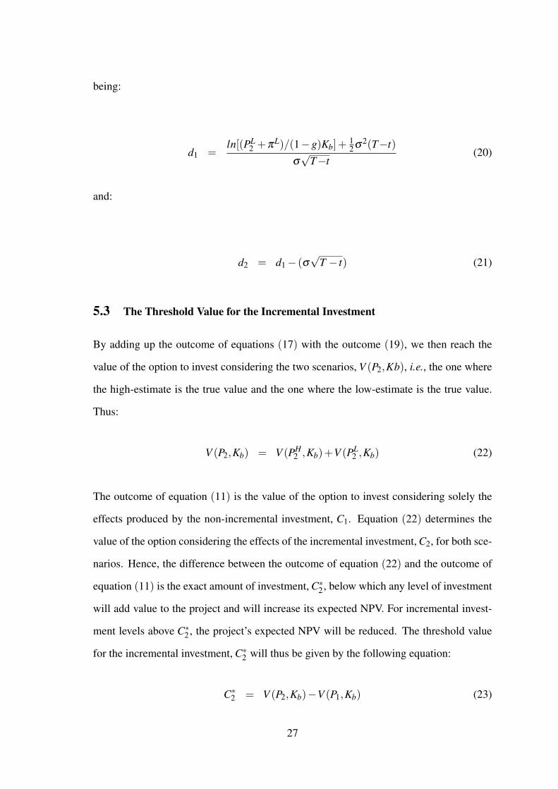
5.3 The Threshold Value for the Incremental Investment

By adding up the outcome of equations (17) with the outcome (19), we then reach the

value of the option to invest considering the two scenarios, V (P2,Kb), i.e., the one where

the high-estimate is the true value and the one where the low-estimate is the true value.

Thus:

V (P2,Kb) = V (PH2 ,Kb)+V (PL

2 ,Kb) (22)

The outcome of equation (11) is the value of the option to invest considering solely the

effects produced by the non-incremental investment, C1. Equation (22) determines the

value of the option considering the effects of the incremental investment, C2, for both sce-

narios. Hence, the difference between the outcome of equation (22) and the outcome of

equation (11) is the exact amount of investment, C∗2 , below which any level of investment

will add value to the project and will increase its expected NPV. For incremental invest-

ment levels above C∗2 , the project’s expected NPV will be reduced. The threshold value

for the incremental investment, C∗2 will thus be given by the following equation:

C∗2 = V (P2,Kb)−V (P1,Kb) (23)

27

The ratio between the incremental investment threshold and the base construction costs is

given by the following equation:

RC∗2 =C∗2Kb

(24)

Part III

Numerical Example

5.4 The Base Case

The following table includes information about the inputs used in the present numerical

example:

Table 1: inputs: description and values

Inputs Description Values

Kb base construction costs USD 100,000,000

σ standard deviation 0.25

T − t “time to expiration” 0.5 (years)

n calibration parameter of W(P,K) 10

b calibration parameter of W(P,K) ln(1/0.5)

g penalty costs 0.02

pHA high-value estimate for the additional revenues USD 30,000,000

kHA high-value estimate for the additional costs USD 15,000,000

pLA low-value estimate for the additional revenues USD 9,000,000

kLA low-value estimate for the additional costs USD 6,000,000

θ probability of occurrence of the high-value estimate 0.5

(1−θ) probability of occurrence of the low-value estimate 0.5

Using the inputs listed above and applying the model described in Part II, we have reached

28

the following outputs:

Table 2: outputs: description, values and corresponding equations

Outputs Description Values Equation

Pb base price USD 101,756,344 (5)

πH additional profit considering the high-value estimate USD 15,000,000 (6)

πL additional profit considering the low-value estimate USD 3,000,000 (7)

E(π) expected value for the additional profit USD 9,000,000 (8)

P1 optimal price after investing C1 USD 98,743,325 (9)

W (P1,Kb) probability of winning with price P1 54.29% (10)

V (P1,Kb) value of the option after investing C1 USD 6,773,641 (11)

PH2 optimal price considering the high-value estimate USD 96,955,641 (14)

V (PH2 ,Kb)θ option value considering the high-value estimate USD 4,767,489 (17)

PL2 optimal price considering the low-value estimate USD 100,700,095 (18)

V (PL2 ,Kb)(1−θ) option value considering the low-value estimate USD 2,257,852 (19)

V (P2,Kb) option value considering both estimates USD 7,025,341 (22)

C∗2 incremental investment threshold value USD 251,700 (23)

RC∗2 ratio “investment threshold / base construction costs” 0.25% (24)

5.5 Sensitivity Analysis

5.5.1 Is There a Scale-Effect?

Considering that the size of a construction project is given by the dimension of its base

construction costs, Kb, we performed a sensitivity analysis with the purpose of verifying

if a scale-effect is present, i.e., if the investment threshold ratio, RC∗2 assumes different

values in response to variations in the level of the base construction costs. We defined

two alternative scenarios, where (i) the amount of the base construction costs are twice

as great and four times as great as in the base case, i.e., equal to USD 200,000,000 and

USD 400,000,000, (ii) the level for the high-value estimate and the low-value estimate of

the additional profit respects this same proportion and (iii) the corresponding probabilities

29

of occurrence remain unchanged. We reached the following results for the incremental

investment threshold value, C∗2 and for the incremental investment threshold ratio, RC∗2 :

Table 3: sensitivity analysis: scale-effect

(for: σ = 0.25; T − t = 0.5; n = 10; b = ln(1/0.5); g = 0.02)

base case alternative scenario 1 alternative scenario 2

Kb USD 100,000,000 USD 200,000,000 USD 400,000,000

πH USD 15,000,000 USD 30,000,000 USD 60,000,000

πL USD 3,000,000 USD 6,000,000 USD 12,000,000

θ 50% 50% 50%

(1−θ) 50% 50% 50%

ε(π) USD 9,000,000 USD 18,000,000 USD 36,000,000

C∗2 USD 251,700 USD 503,400 USD 1,006,800

RC∗2 0.25% 0.25% 0.25%

Results included in Table 3 clearly demonstrate that the investment threshold is propor-

tional to the amount of the base construction costs, which means that no scale-effect

is present. In fact, for the three different dimensions considered, the ratio between the

threshold and the base construction costs remains constant and equal to 0.25%. Thus,

these results express the existence of a linear relationship between the incremental invest-

ment threshold value and the base construction costs.

5.5.2 The Impact of Different Levels of Probabilities Associated with the High/Low

Value Estimates

The results concerning the impact of considering different levels for the probabilities as-

sociated with the high-value and the low-value estimates in the model’s outcome are in-

cluded in Table 4.

30

Table 4: sensitivity analysis: probabilities associated with high/low value estimates

(for information about the inputs considered, please refer to Table 1)

θ (1−θ) E(π) V (P1,Kb) V (P2,Kb) C∗2 RC∗2

99% 1% USD 14,880,000 USD 9,475,025 USD 9,484,785 USD 9,760 0.01%

90% 10% USD 13,800,000 USD 8,943,931 USD 9,033,050 USD 89,119 0.09%

80% 20% USD 12,600,000 USD 8,345,927 USD 8,531,123 USD 185,196 0.19%

70% 30% USD 11,400,000 USD 7,819,379 USD 8,029,196 USD 209,817 0.21%

60% 40% USD 10,200,000 USD 7,286,518 USD 7,527,268 USD 240,750 0.24%

50% 50% USD 9,000,000 USD 6,773,641 USD 7,025,341 USD 251,700 0.25%

40% 60% USD 7,800,000 USD 6,280,981 USD 6,523,414 USD 242.433 0.24%

30% 70% USD 6,600,000 USD 5,808,732 USD 6,021,487 USD 212.755 0.21%

20% 80% USD 13,800,000 USD 5,357,042 USD 5,519,559 USD 162.517 0.16%

10% 90% USD 5,400,000 USD 4,926,015 USD 5,017,632 USD 91,617 0.09%

1% 99% USD 4,200,000 USD 4,555,803 USD 4,565,898 USD 10,095 0.01%

Results included in Table 4 clearly show that, the closer the probabilities are to the up-

per limit or the lower limit, the smaller is the investment threshold value. This is due

to the fact that, the closer the probability levels are to 100% or to 0%, the lower is the

uncertainty regarding which will be the true value, meaning that the level of incremental

investment needed that is needed to eliminate that level of uncertainty is smaller. The two

more extreme scenarios clearly reflect such: when parameter θ equals 99% or 1%, the in-

vestment threshold assumes very low values (USD 9,760 and USD 10,095, respectively).

On the contrary, as probabilities tend to 50%, the higher is the threshold value, C∗2 . Thus,

threshold value reaches its maximum when the level of uncertainty is the highest, i.e.,

when the probabilities associated with the two estimates assume the same value.

31

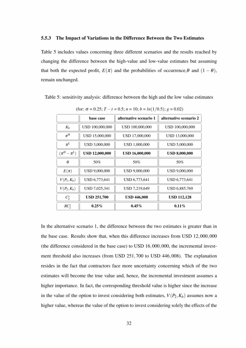
5.5.3 The Impact of Variations in the Difference Between the Two Estimates

Table 5 includes values concerning three different scenarios and the results reached by

changing the difference between the high-value and low-value estimates but assuming

that both the expected profit, E(π) and the probabilities of occurrence,θ and (1− θ),

remain unchanged.

Table 5: sensitivity analysis: difference between the high and the low value estimates

(for: σ = 0.25; T − t = 0.5; n = 10; b = ln(1/0.5); g = 0.02)

base case alternative scenario 1 alternative scenario 2

Kb USD 100,000,000 USD 100,000,000 USD 100,000,000

πH USD 15,000,000 USD 17,000,000 USD 13,000,000

πL USD 3,000,000 USD 1,000,000 USD 5,000,000

(πH −πL) USD 12,000,000 USD 16,000,000 USD 8,000,000

θ 50% 50% 50%

E(π) USD 9,000,000 USD 9,000,000 USD 9,000,000

V (P1,Kb) USD 6,773,641 USD 6,773,641 USD 6,773,641

V (P2,Kb) USD 7,025,341 USD 7,219,649 USD 6,885,769

C∗2 USD 251,700 USD 446,008 USD 112,128

RC∗2 0.25% 0.45% 0.11%

In the alternative scenario 1, the difference between the two estimates is greater than in

the base case. Results show that, when this difference increases from USD 12,000,000

(the difference considered in the base case) to USD 16,000,000, the incremental invest-

ment threshold also increases (from USD 251,700 to USD 446,008). The explanation

resides in the fact that contractors face more uncertainty concerning which of the two

estimates will become the true value and, hence, the incremental investment assumes a

higher importance. In fact, the corresponding threshold value is higher since the increase

in the value of the option to invest considering both estimates, V (P2,Kb) assumes now a

higher value, whereas the value of the option to invest considering solely the effects of the

32

non-incremental investment, V (P1,Kb) remains unchanged. On the contrary, for a smaller

difference between the two estimates (USD 8,000,000), as the results reached for the

alternative scenario 2 clearly reflect, the investment threshold is smaller: USD 112,128,

compared to USD 251,700, in the base case. The level of uncertainty associated with the

two estimates is now lower and this lower level of uncertainty is reflected in the value of

option to invest considering both estimates, V (P2,Kb). The value of this option is, in the

alternative scenario 2, smaller than in the other two cases and thus closer to the value of

the option to invest considering only the investment in C1, V (P1,Kb), whose value does

not depend upon the differences between the two estimates, since the expected value for

the additional profit, E(π) remains unchanged.

We thus conclude that, the higher (lower) the difference between the high-value estimate

and the low-value estimate, the higher (lower) will be the uncertainty concerning which

estimate will become the true value, and the higher (lower) will be the value of the option

to invest considering the two estimates, V (P2,Kb). Consequently - since the value of the

option to invest considering only the effects of the non-incremental investment, V (P1,Kb)

remains unchanged - the higher (lower) will be the value for investment threshold, C∗2 ,

and the higher (lower) will be the value of the ratio, RC∗2 .

Part IV

Concluding Remarks

Several types of uncertainty surround construction projects and construction companies

should proactively manage the effects they may produce in the project’s final NPV. We

approached a specific type of uncertainty and designated it as “volume uncertainty”. This

type of uncertainty is critical since, at least frequently, managers do not know with pre-

cision the amount of work they will be executing throughout the project’s life cycle and,

consequently, the expected final profit the project will generate. To assess the impact of

33

volume uncertainty on the project’s final NPV, we defined a discrete-time stochastic vari-

able and designated it as “additional value”. Additional value is the value that is hidden

in the the most uncertain parts of the project and, in the context of the present research,

is defined as the one that does not derive from merely executing the tasks specified in the

bid documents.

To capture and quantify this type of hidden-value, construction companies need to invest.

Initially, by only using the skills of his or her own experienced staff, construction man-

agers are able to define a high-value estimate and a low-value estimate for the additional

profit, and to stipulate a probability of occurrence to each of the estimates. Based on the

numerical solution proposed by Ribeiro et al. (2013), we suggested a model which led

us to conclude that managers will produce a more competitive bid even if no incremental

investment is undertaken, since the optimal price that results from the expected profit de-

termined just by undertaking a preliminary analysis of the bid documents is greater than

the base price, i.e., the optimal price in the absence of any recognition and quantification

of hidden-value. However, in order to resolve the uncertainty concerning which of the

two estimates will become the true value for the expected additional profit, contractors

often need to invest in human capital and technology and, hence, hire specialized firms

and highly skilled professionals. The outcome of our model is the threshold value for

this incremental investment. Therefore, managers may apply a simple decision rule: hire

external services with the purpose of resolving the uncertainty concerning which of the

two estimates previously established is the true value, provided that the cost of the incre-

mental investment in human capital and technology does not exceed the threshold value

previously determined. Any amount paid for external services, which is lower than the

threshold value, will increase the project’s expected NPV and, the lower this cost is, the

higher will be the increase in the project’s expected NPV. On the contrary, if the amount

actually invested exceeds the predetermined threshold value, then the project’s expected

NPV will be reduced. The model also model determines the optimal bid price in the case

the true value reached by undertaking the incremental investment equals the high-estimate

34

for the additional value and also in the case the true value equals the low-estimate, both

previously established.

Sensitivity analysis revealed that the threshold value responds linearly to variations in

the investment size, which means that no scale-effect is present in the model. Sensitivity

analysis also showed that, the closer to 50% is the probability of occurrence associated

with the estimates, the greater the threshold value needs to be, since undertaking the in-

cremental investment assumes a higher importance in response to the presence of higher

levels of uncertainty regarding which of the two estimates will become the true value.

Finally, sensitivity analysis performed to the distance between the two estimates demon-

strated that, the more distant the two estimates defined for the additional value are from

each other, the greater the incremental investment threshold value needs to be, since con-

tractors face more uncertainty over which of the two estimates will be the true value. The

decision of undertaking the incremental investment becomes, therefore, more important

and such higher importance is reflected in a greater threshold value. On the contrary, if

the two estimates are closer to each other, then the threshold value is lower, since the

level of uncertainty surrounding the two estimates is, now, also lower. Hence, the deci-

sion of undertaking the incremental investment assumes less importance and this smaller

importance is reflected in a lower value for the incremental investment threshold.

35

References

Adrian, J. J.: (1993), Construction Claims: A Quantitative Approach. New Jersey: Prentice-Hall.

Akintoye, A. and E. Fitzgerald: (2000), ‘A Survey of Current Cost Estimating Practices’. Con-

struction Management and Economics Vol. 18, Nº 2, 161–72.

Arditi, D. and R. Chotibhongs: (2009), ‘Detection and Prevention of Unbalanced Bids’. Construc-

tion Management and Economics Vol. 27, Nº 8, 721–732.

Chao, L. and C. Liu: (2007), ‘Risk Minimizing Approach to Bid-Cutting Limit Determination’.

Construction Management and Economics Vol. 25, Nº 8, 835–843.

Chapman, C., S. Ward, and J. Bennell: (2000), ‘Incorporating Uncertainty in Competitive Bid-

ding’. International Journal of Project Management Vol.18, Nº 5, 337–347.

Cheung, S. O., P. Wong, A. Fung, and W. Coffey: (2008), ‘Examining the Use of Bid Information

in Predicting the Contractor Performance’. Journal of Financial Management of Property and

Construction Vol. 13, Nº 2, 111–122.

Christodoulou, S.: (2010), ‘Bid Mark-Up Selection Using Artificial Neural Networks and an En-

tropy Metric’. Engineering Construction and Architectural Management Vol. 17, Nº 4, 424–

439.

Clough, R., G. Sears, and K. Sears: (2000), Construction Project Management. New York: John

Wiley & Sons, Inc.

Davinson, P.: (2003), Evaluating Contract Claims. Oxford, UK: Blackwell Publishing.

Drew, D. and M. Skitmore: (1997), ‘The Effect of Contract Type and Contract Size on Competi-

tiveness in Construction Contract Bidding’. Construction Management and Economics Vol. 15,

Nº 5, 469–489.

Drew, D., M. Skitmore, and H. Lo: (2001), ‘The Effect of Client and Size and Type of Construction

Work on a Contractor Bidding Strategy’. Building Envirnoment Vol. 36, Nº 3, 393–406.

36

Dyer, D. and J. Kagel: (1996), ‘Bidding in Common Value Auctions: How the Commercial Con-

struction Industry Corrects for the Winners Curse’. Management Science Vo. 42, Nº 10, 1463–

1475.

Fayek, A.: (1998), ‘Competitive Bidding Strategy Model and Software System for Bid Prepara-

tion’. Journal of Construction Engineering and Management Vol. 124, Nº 1, 1–10.

Ford, D., D. Lander, and J. Voyer: (2002), ‘A Real Options Approach to Valuing Strategic Flexi-

bility in Uncertain Construction Projects’. Construction Management and Economics Vol. 20,

Nº 4, 343–351.

Halpin, D. and B. Senior: (2011), Construction Management. New Jersey: John Wiley & Sons,

Inc., 4th edition.

Kim, H. and K. Reinschmidt: (2006), ‘A Dynamic Competition Model for Construction Contrac-

tors’. Construction Management and Economics Vol. 24, Nº 9, 955–965.

Kululanga, G. K., W. Kuotcha, R. McCaffer, and F. Edum-Fotwe: (2001), ‘Construction Con-

tractors Claim Process Framework’. Journal of Construction Engineering and Management

Vol.127, Nº 4, 309–314.

Laryea, S.: (2011), ‘Quality of Tender Documents: Case Studies from the U.K.’. Construction

Management and Economics Vol. 29, Nº 3, 275–286.

Laryea, S. and W. Hughes: (2008), ‘How Contractor Price Risk in Bids: Theory and Practice’.

Construction Management and Economics Vol. 26, Nº 9, 911–924.

Li, H. and P. Love: (1999), ‘Combining Rule-Based Expert Systems and Artificial Neural Net-

works for Mark-Up Estimation’. Construction Management and Economics Vol. 17, Nº 2,

169–176.

Liu, M. and Y. Ling: (2005), ‘Modeling a Contractor Mark-Up Estimation’. Journal of Construc-

tion Engineering and Management Vol. 131, Nº 4, 391–399.

Mak, S. and D. Picken: (2000), ‘Using Risk Analysis to Determine Construction Project Contin-

gencies’. Journal of Construction Engineering and Management Vol. 126, Nº 3, 130–136.

37

Margrabe, W.: (1978), ‘The Value of an Option to Exchange One Asset for Another’. The Journal

of Finance Vol. 33, Nº 4, 177–186.

Mattar, M. and C. Cheah: (2006), ‘Valuing Large Engineering Projects under Uncertainty: Private

Risk Effects and Real Options’. Construction Management and Economics Vol. 24, Nº 8, 847–

860.

Mohamed, K., S. Khoury, and S. Hafez: (2011), ‘Contractors Decision for Bid Profit Reduction

Within Opportunistic Bidding Behavior of Claims Recovery’. International Journal of Project

Management Vol. 29, Nº 1, 93–107.

Ng, F. and H. Bjornsson: (2004), ‘Using Real Options and Decision Analysis to Evaluate Invest-

ments in the Architecture, Construction and Engineering Industry’. Construction Management

and Economics Vol. 22, Nº 5, 471–482.

Ngai, S., D. Drew, H. Lo, and M. Skitmore: (2002), ‘A Theoretical Framework for Determin-

ing the Minimum Number of Bidders in Construction Bidding Competitions’. Construction

Management and Economics Vol. 20, Nº 6, 473–482.

Pinnell, S. S.: (1998), How To Get Paid for Construction Changes: Preparation, Resolution Tools

and Techniques. New York: McGraw-Hill.

Ribeiro, J. A., P. J. Pereira, and E. Brandão: (2013), ‘Reaching an Optimal Mark-Up Bid through

the Valuation of the Option to Sign the Contract by the Selected Bidder’. Available at SSRN:

http://ssrn.com/abstract=2265862 pp. 1–38.

Rooke, J., D. Seymour, and R. Fellows: (2004), ‘Planning for Claims: an Ethnography of Industry

Culture’. Construction Management and Economics Vol. 22, Nº 6, 655–662.

Skitmore, M.: (2002), ‘Predicting the Probability of Winning Sealed Bid Auctions: A Comparison

of Models’. The Journal of the Operational Research Society Vol. 53, Nº 1, 47–56.

Tan, Y., L. Shan, A. Khlaled, and S. Song: (2008), ‘An Examination of the Factors Affecting

Contractors Competition Strategy: a Hong Kong Sudy’. International Journal of Project Or-

ganisation and Management Vol. 1, Nº1, 4–23.

38

Tenah, K. and C. Coulter: (1999), ‘Bid Mark-Up Metodologies’. Cost Engineering Vol. 41, Nº

11, 39–44.

Thomas, R.: (2001), Construction Contract Claims. New York: Palgrave, 2nd Edition.

Wallwork, J.: (1999), ‘Is There a Right Price in Construction Bids?’. Cost Engineering Vol. 40,

Nº 2, 41–43.

Woodward, J. F.: (1997), Construction Project Management: Getting It Right First Time. ,London:

Thomas Telford.

Yiu, C. Y. and C. S. Tam: (2006), ‘Rational Under-Pricing in Bidding Strategy: A Real Options

Model’. Construction Management and Economics Vol. 24, Nº 5, 475–484.

39