CE790 Directed Research A Report on Nonstationary...

CE790

Directed Research

A Report on Nonstationary Response of

Nonlinear MDOF Systems using Equivalent Linearization

and Compact Analytical Model of the Excitation Process

by Baris Erkus 1

supervised by Prof. Dr. Sami F. Masri

27 October 2003

1Ph.D. Student, Civil Engineering Dept., University of Southern California, [email protected]

Contents

1 A Review of Random Processes 11.1 Introduction . . . . . . . . . . . . . . . . . . . . . . . . . . . . . . . . . . . . . . . . . 11.2 Probability . . . . . . . . . . . . . . . . . . . . . . . . . . . . . . . . . . . . . . . . . 11.3 Random Variables . . . . . . . . . . . . . . . . . . . . . . . . . . . . . . . . . . . . . 11.4 The Gaussian Distribution . . . . . . . . . . . . . . . . . . . . . . . . . . . . . . . . . 31.5 Random Processes . . . . . . . . . . . . . . . . . . . . . . . . . . . . . . . . . . . . . 4

1.5.1 Stationary Random Processes . . . . . . . . . . . . . . . . . . . . . . . . . . . 51.5.2 Cross-Correlation Function . . . . . . . . . . . . . . . . . . . . . . . . . . . . 61.5.3 Derivatives of Stationary Processes . . . . . . . . . . . . . . . . . . . . . . . . 61.5.4 Spectral properties of Stationary Random Processes . . . . . . . . . . . . . . 71.5.5 Narrowband, Wideband and White Noise Processes . . . . . . . . . . . . . . 9

1.6 Stochastic Response of Linear Systems . . . . . . . . . . . . . . . . . . . . . . . . . . 9

2 Nonstationary Response of Nonlinear MDOF Systems 112.1 Introduction . . . . . . . . . . . . . . . . . . . . . . . . . . . . . . . . . . . . . . . . . 112.2 A Compact form of Nonstationary Excitation Covariance . . . . . . . . . . . . . . . 11

2.2.1 Eigenvector Expansion of Covariance Matrix . . . . . . . . . . . . . . . . . . 112.2.2 Orthogonal Chebyshev Polynomials Representation of Covariance Matrix . . 12

2.3 Statical Linearization Method for Nonstationary Excitation . . . . . . . . . . . . . . 132.4 Linearized Equations for Compact Form of the Excitation Covariance Kernel . . . . 152.5 A Numerical Example: Duffing Oscillator . . . . . . . . . . . . . . . . . . . . . . . . 17

2.5.1 Governing Equations for Duffing Oscillator . . . . . . . . . . . . . . . . . . . 182.5.2 Random Excitation and Covariance Kernel . . . . . . . . . . . . . . . . . . . 192.5.3 Numerical Solution Technique and Mathematica Source code . . . . . . . . . 192.5.4 Monte-Carlo Simulation and Mathematica Source Code . . . . . . . . . . . . 232.5.5 Results . . . . . . . . . . . . . . . . . . . . . . . . . . . . . . . . . . . . . . . 262.5.6 Conclusion . . . . . . . . . . . . . . . . . . . . . . . . . . . . . . . . . . . . . 27

1

Abstract

This report is a fruit of the effort to learn the fundamental concepts of random processes andrandom vibrations theory under the course “CE790, Directed Research”. The boundaries, however,extended to more advanced topics such as equivalent linearization and nonstationary responses. Thegoal was to review the paper by Smyth and Masri on nonstationary analysis of nonlinear structuresand implement one of the examples given in that paper using Mathematica. The main challengewas not the main theory as may be expected. Indeed, the paper is very clear to understand and thetheory is easy to follow. The challenge was the implementation in Mathematica. The inefficiencyof Mathematica in writing highly numerical codes was extremely restricted the author from furtherprogress. The preparation of this report took more time than expected, however, the author hasgained a lot of knowledge on the topic under the supervision of Prof. Dr. Sami F. Masri for astand-alone research that will be carried out later.

This report consists of two parts: The first part is a brief review of theory of random processes.The explanations are straightforward and very helpful for a review. The second section is the reviewof the theory explained in the aforementioned paper. Although it looks similar to the original paper,some parts uses different nomenclature and, details of some of the sections are added. In additionto the original theory, a simplification of the method proposed is given. This simplified approach iseasier to implement than the original approach. Finally a Mathematica code is given as an exampleof the application of the method.

The only benefit of Mathematica was the use of built-in approximation function, namely “Fit”.Other than that, the differential equation solver of Mathematica was not able to solve the equationsobtained and, therefore, a Runge-Kutta solver is coded. At the time of preparation of this documenta new version of Mathematica (Version 5.0.0) is released. This version is capable of solving multisingle degree differential equations using Runge-Kutta method. However, it may be useful to useother programming languages such as Matlab for the numerical computation to avoid the otherproblems of Mathematica, which were explained in this report.

The author wish to thank to Prof. Masri, for his supervision. The work was extremely helpfulto the student to understand the concepts that appear very frequently in the field, and it willdefinitely be extended in the future.

Chapter 1

A Review of Random Processes

1.1 Introduction

This chapter reviews the basic concepts of probability theory and random processes to establisha foundation for the stochastic analysis of linear and nonlinear systems. In particular, responsestatistics of a system under a stationary excitation is investigated. Roberts and Spanos (1990) isused as the main reference. Definitions given herein are considerably brief and, interested reader isdirected to textbooks on these topics such as Papoulis (1984) for more explanations.

1.2 Probability

Theory of probability is characterized with three fundamental axioms.

Axiom 1.2.1. Let A be a random event and P (A) be the probability that event A occurs. Then,

0 6 P (A) 6 1 (1.1)

Axiom 1.2.2. Let S be the event that any event in the sample space occurs, that is certain event.Then,

P (S) = 1 (1.2)

Axiom 1.2.3. Let A and B are mutually exclusive. Then

P (A ∪B) = P (A) + P (B) and P (A ∩B) = ∅ (1.3)

If A and B are not mutually exclusive. Then

P (A ∪B) = P (A) + P (B)− P (A ∩B) (1.4)

Probability of an event may be defined as a mapping of the possible events of sample space into[0, 1].

1.3 Random Variables

For a complete set of exclusive events, each event can be associated with a number, say η,which is called as random variable. In some cases η takes only a finite number of distinct values

1

CE790 Directed Research: Nonstationary Response of MDOF Nonlinear Systems 2

if underlying events are finite. It may be also continuous and may take any number between −∞and +∞ if underlying events are infinite.

In most of the problems, use of more than one random variable associated with different samplespaces is required. These random variables are formulated as a vector, η = [η1, η2, · · · , ηn].

Definition 1.3.1. Joint distribution function of a random vector η is defined as

Fη(x) = Pη(η 6 x). (1.5)

Properties of joint distribution function can be summarized as follows: Fη(x) → 0 as anyelement of x approaches zero and Fη(x) → 1 as all elements of x approach to +∞. Also, Fη(x)increases monotonically in all variables.

Definition 1.3.2. Joint density function of a random vector η is defined as

fη(x) = f(x1, x2, · · · , xn) =∂nFη(x1, x2, · · · , xn)

∂x1∂x2 · · · ∂xn(1.6)

Due to the probability axioms, fη(x) > 0. Also, the probability that the random vector η fallsin some region R is equal to

Pη(η ∈ R) =

∫Rfη(x)dx. (1.7)

If the individual random variables are independent, i.e.

Pη(η > x) = Pη(η1 > x1)Pη(η2 > x2) · · ·Pη(ηn > xn), (1.8)

then

Fη(x) = F1(x1)F2(x2) · · ·Fn(xn) (1.9)

fη(x) = f1(x1)f2(x2) · · · fn(xn) (1.10)

where Fk(xk) and fk(xk) are distribution and density functions of variable ηk, respectively.Consider two random variables, η and ρ related through the equation

ρ = g(η). (1.11)

Then, the density function fρ(y) of ρ is related with the density function fη(x) of η as follows:

fρ(y) =

m∑i=1

fη(xi)|d

dxg(xi)| (1.12)

where xi, (i = 1, 2, · · · ,m) are the roots of y = g(x).Equation (1.11) can also be used for random vectors. If two random vectors are related with

the matrix transformation given byρ = g(η), (1.13)

then the relation between two density functions is given as follows:

fρ(y) = fη(x)|J |x=g(y). (1.14)

where,

J =

∣∣∣∣∣∣∣∂g1∂y1

∂g1∂y2

· · · ∂g1∂yn

...∂gn∂y1

∂gn∂y2

· · · ∂gn∂yn

∣∣∣∣∣∣∣ . (1.15)


Definition 1.3.3. Lets η be a random vector and g(η) is a matrix function of η. Expectation ofg(η) is defined by

E[g(η)] =

∫ x=+∞

x=−∞g(η)fη(x)dx (1.16)

Definition 1.3.4. Covariance matrix of η is defined as

K = E[(η −m)(η −m)T ] (1.17)

where m = E[η]. In this definition g(η) = (η −m)(η −m)T .

Diagonal terms of K are called as variances of each of the individual random variable:

var(ηi) = σ2i = E[(ηi −mi)(ηi −mi)] = E[(ηi −mi)

2] (1.18)

Definition 1.3.5. Correlation (or autocorrelation) matrix of η is defined as

R = E[ηηT ] (1.19)

In this definition g(η) = ηηT .

Detailed treatment of covariance and correlation matrices can be found in Stark and Woods(2002), pages 251-258.

Definition 1.3.6. Characteristic function is defined as

Θη(ω) = E[eiωTη] =

∫ x=+∞

x=−∞eiω

Tηfη(x)dx. (1.20)

In this definition g(η) = g(η) = eiωTη

Clearly characteristic function is multi dimensional Fourier transform of fη(x)1.

1.4 The Gaussian Distribution

The Gaussian probability distribution of a random vector η is given by

fη(x) =1

(2π)n/2|K|1/2e−

12(x−m)TK−1(x−m). (1.21)

The characteristic function is given by

Θη(ω) = eimTω− 1

2ωTKω. (1.22)


t

t

t

η1(t)

η2(t)

ηn(t)

.

.

.

}samplefunction

t1 t2

Figure 1.1: Ensemble of Random Process

1.5 Random Processes

In the previous section, a random variable is defined as a number that is associated with anevent. In most of the cases, outcome of an event is a function of several variables. This functionis called a realization or a sample function. The collection of all possible outcomes is called theensemble of the random process. An example of a random process with the n-sample functions ofa single variable is given by figure 1.1, which is the case for most of the engineering problems.

Now, lets take the points from each sample function for a fixed time, t = t1. The collectionof these n points is actually the set of possible outcomes of a random variable as each outcomeis associated with the value of the function at this particular time i.e. η = η(t1). As one canobserve, for the random process given by figure 1.1, there are infinite number of random variableswhich forms a random vector with an infinite dimension. Hence, all the definitions given in theprevious sections for random variables are applicable for the random process given by figure 1.1. Forexample, random variable that is obtained by fixing the time to t1 has a probability distribution.Also the random variable at time t2 has a probability distribution. There is also a joint probabilitydistribution of these two random variables, which results the 2-by-2 covariance and autocorrelationmatrices.

In this report, the notation used for a random vectors will be also used for the random processes,η. However, we should keep in mind that random vector elements are finite and random processelements are infinite. Therefore while we talk about the ith element of a random vector, we mentionthe random variable at time t for random processes and denote it as η(t).

1Definition of the Fourier Transform is not given here as it will be defined later in this report


1.5.1 Stationary Random Processes

Different from a random vector, a random process has an infinite number of probability anddistribution functions, which makes the interpretation of the random processes difficult as onecannot deal with infinite number of distinct probability definitions. A good practice is to use someassumptions to reduce such a complex problem into a simpler one. For example, one may assumethat random variables at any times ti and tj have the same probability definitions. Furthermoreassume that joint probability distribution of the two random variables at any times ti and tj aresame as the joint probability of the two random variables at any times tk and tl, if ti − tj = tk − tl.A random process, where above assumptions hold, is known as stationary random process of ordertwo. It follows that for a second order stationary random process any two random variables at timeti, tj , tk and tl have the same mean and the correlation between ti and tj is same as the correlationbetween tk and tl.

The question at this point is that, is a random process stationary if random variables at time ti,tj , tk and tl have the same mean and the correlation between the random variables at times ti andtj is same as the correlation between the random variables at times tk and tl when ti− tj = tk − tl?The answer is no; as for such a process, probability distributions of the random variables at ti,tj , tk and tl and joint probabilities defined above may be different. The latter random process isknown as wide sense stationary (WSS), while the former one is known as strict sense stationary(SSS). Here more formal definitions of these terms are given.

Definition 1.5.1. A random process is called strict-sense stationary (SSS) if its spectral propertiesare invariant to a time shift, i.e. the two random processes η(t) and η(t+c) have the same statisticsfor any c.

First-order statistics of SSS processes are independent of time and can be abbreviated asf(η; t) = f(η). Similarly, joint probability function f(η1,η2; t1 + c, t2 + c) is independent of cand is abbreviated as

f(η1,η2; t1, t2) = f(η1,η2; τ), τ = t1 − t2. (1.23)

As natural consequences of these properties, for a SSS process, mean of the random variable isconstant for all time, t and abbreviated as E[η(t)] = m(t) = m. Correlation and covariance of thetwo random variables η(t1) and η(t2) depends only τ = t1− t2 and abbreviated as R(τ) and K(τ).The relation between these parameters is

R(τ) = K(τ) +m2 (1.24)

Definition 1.5.2. A random process is called wide-sense stationary (WSS) if its mean is constant

E[η(t)] = m(t) = m (1.25)

and the correlation between the random variables at times t1 and t2 depends only only τ = t1 − t2i.e.

E[η(t1)ηT (t2)] = R(t1 − t2) = R(τ). (1.26)

These assumptions are not valid for real-life events, yet they form a sound background for theanalysis of more complex problems.


Definition 1.5.3. The temporal averages of a sample function is defined as

< η(t) >= limT→∞

1

T

∫ T

0η(t)dt, (1.27)

< η(t)η(t+ τ) >= limT→∞

1

T − τ

∫ T−τ

0η(t)η(t+ τ)dt. (1.28)

It should be noted that the temporal averages of a sample function is different then the meanvalue and correlation of SSS and WSS random processes. The mean value and correlation arecomputed using whole set of sample functions and known as ensemble averages. A special caseoccur when the temporal averages of all sample functions and the ensemble averages of a stationaryrandom process are equal.

Definition 1.5.4. A stationary random process is called ergodic in the mean if

< η(t) >= E[η(t)] = m, for all i = 1, · · · , n. (1.29)

Definition 1.5.5. A stationary random process is called ergodic in the correlation if

< η(t)η(t+ τ) >= E[η(t)η(t+ τ)] = R(τ), for i = 1, · · · , n. (1.30)

1.5.2 Cross-Correlation Function

Definition 1.5.6. Cross-correlation function of two random processes is defined as

Rηρ(t1, t2) = E[η(t1)ρ(t2)]. (1.31)

If the processes η(t) and ρ(t) are stationary, the cross-correlation function depends only on τi.e.,

Rηρ(τ) = E[η(t+ τ)ρ(t)]. (1.32)

It should be noted that the the order of the subscripts determine the definition of cross-correlation.For example, the cross-correlation

Rρη(τ) = E[ρ(t+ τ)η(t)] (1.33)

is different than Rηρ(τ). In fact, for stationary random processes Rηρ(τ) = Rρη(−τ) (Wirschinget al. (1995))

1.5.3 Derivatives of Stationary Processes

The cross-correlation between a stationary random process and its derivative is of special inter-est. consider the derivative of correlation function,

d

dτRη(τ) =

d

dτE[η(t+ τ)η(t)]

= E[d

dτη(t+ τ)η(t)]

= E[η(t+ τ)η(t)]

= Rηη(τ). (1.34)


Therefore the first derivative of correlation function is the cross-correlation function between η(t)and η(t). Correlation of the derivative of the stationary random process is found as

d2

dτ2Rη(τ) =

d

dτE[η(t+ τ)η(t)]

=d

dτE[η(t)η(t− τ)]

= E[η(t)(−η(t− τ))]

= −Rη(τ). (1.35)

1.5.4 Spectral properties of Stationary Random Processes

The correlation function of a stationary random process is a time-domain function. It is usefulto define this function in terms of some eigenfunctions such as sines and cosines. For this purposeFourier transformation is used. Here, Fourier transformation that will be used throughout thispaper is given first as there are different definitions of Fourier transformation in various literature.

Definition 1.5.7. The Fourier transform of a function f(t) is defined as

F (ω) =

∫ ∞

−∞f(t)e−iωtdt. (1.36)

Similarly the inverse Fourier transform is defined as

f(t) =1

2π

∫ ∞

−∞F (ω)eiωtdω. (1.37)

Definition 1.5.8. The power spectral density (psd) function of a stationary random process is theFourier transform of correlation function,

S(ω) =

∫ ∞

−∞R(τ)e−iωτdτ. (1.38)

The correlation function is found taking the inverse Fourier transform of the psd function,

R(τ) =1

2π

∫ ∞

−∞S(ω)eiωτdω. (1.39)

If the random process is real, R(τ) is real and even. Similarly S(ω) is real and even. In thiscase, the Fourier transform pair reduces to

S(ω) =

∫ ∞

−∞R(τ)cos(ωτ)dτ = 2

∫ ∞

0R(τ)cos(ωτ)dτ (1.40)

R(τ) =1

2π

∫ ∞

−∞S(ω)cos(ωτ)dω =

1

π

∫ ∞

0S(ω)cos(ωτ)dω. (1.41)

Equations (1.38), (1.39), (1.40) and (1.41) are known as Wiener-Khinchine relations.It is observed that given the psd, mean square value of a stationary random process can be

found as

R(0) =1

π

∫ ∞

0S(ω)dω. (1.42)


R(τ)

−ω0 ω0

ω

S(ω)

τ

(a) Periodic

R(τ)

ω

S(ω)

τ

(b) Narrowband

R(τ)

ω

S(ω)

τ

(c) Wideband

R(τ)

ω

S(ω)

τ

Area = S0

S0

(d) White Noise

Figure 1.2: Classification of the processes according to the frequency content

Definition 1.5.9. The cross-spectral density function of two random processes is defined as

Sηρ(ω) =

∫ ∞

−∞Rηρ(τ)e

−iωτdτ. (1.43)

The cross-correlation function is found taking the inverse Fourier transform of the cross-spectralfunction,

Rηρ(τ) =1

2π

∫ ∞

−∞Sηρ(ω)e

iωτdω. (1.44)

Cross-spectral density function is generally complex even when both processes are real. For allcases, following relations hold:

Sηρ(ω) = Sρη(ω) (1.45)

Rηρ(τ) = Rρη(τ). (1.46)


1.5.5 Narrowband, Wideband and White Noise Processes

Power spectral density provides information about the frequency content of correlation. Fourtypes of psd function is of interest. If the correlation is a periodic function which can be representedby one frequency, psd is a delta function as shown in figure 1.2(a). A process is called narrowbandif its psd has significant values over a narrow frequency range around a central frequency as shownin figure 1.2(b). A process is called as wideband if its psd has significant values over a wide rangeof frequencies as shown in figure 1.2(c). A common idealization of wideband processes is to assumeS(ω) = S0 as shown in figure 1.2(d). In this case, the correlation is a delta function implying thatnor correlation for τ = 0. The correlation is computed as

R(τ) =1

2π

∫ ∞

−∞S0e

iωτdω

=1

2πS0

∫ ∞

−∞eiωτdω

=1

2πS0(2πδ(τ))

= S0δ(τ). (1.47)

1.6 Stochastic Response of Linear Systems

It is known that the response of a linear system, x(t) to an arbitrary excitation, f(t) can befound through convolution

x(t) =

∫ t

0f(λ)g(t− λ)dλ (1.48)

where g(t) is the impulse response. It can be also shown that (Meirovitch (1986)) equation (1.48)can be written as

x(t) =

∫ ∞

−∞f(λ)g(t− λ)dλ =

∫ ∞

−∞f(t− λ)g(λ)dλ. (1.49)

It is also known that that the input-output relation in the frequency domain is given by

X(ω) = G(ω)F (ω) (1.50)

where X(ω), G(ω) and F (ω) are the Fourier transform of input, impulse response function and theexcitation, respectively.

Now lets assume that the excitation is a stationary random process with known statistics. It isknown that the response is also a stationary random process. Lets the mean value of the excitationbe mf . The mean of the response is

mx = mf

∫ ∞

−∞g(λ)dλ = mfG(0). (1.51)

The response autocorrelation function can be derived using the definition given by equation 1.26as follows:

Rx(τ) =

∫ ∞

−∞

∫ ∞

−∞g(λ1)g(λ2)Rf (τ + λ1 − λ2)dλ1dλ2 (1.52)


where Rf is the correlation of the excitation. Power spectral density of the response is the Fouriertransform of the response correlation. A useful relation between the psds of input and output isgiven by

Sx(ω) = |G(ω)|2Sf (ω). (1.53)

Finally the mean square response can be obtained setting τ = 0.

Rx(0) =1

2π

∫ ∞

−∞|G(ω)|2Sf (ω). (1.54)

The detailed derivations of these relations can be found in Meirovitch (1986) and Papoulis (1984).

Chapter 2

Nonstationary Response of NonlinearMDOF Systems

2.1 Introduction

In this chapter, the method proposed by Smyth and Masri (2002) for the stochastic analysisof a class of nonlinear multi-degree-of-freedom systems subjected to nonstationary random exci-tation is reviewed. The covariance kernel of the nonstationary excitation is decomposed into itseigenvalues and eigenvectors, which is known as Karhunen-Loeve (K-L) decomposition. Then, co-variance eigenvectors are approximated by orthogonal Chebyshev polynomials, which results a morecompact form of the covariance matrix. The final excitation covariance is used in the equivalentlinearization analysis of the nonlinear structure. A Duffing oscillator is considered as an example.As the nonstationary excitation covariance, the example given by Traina et al. (1986) is used.

In this study, most of the numerical computations are carried out using the software toolMathematica. Therefore, throughout this report details of the Mathematica code used will begiven when necessary.

2.2 A Compact form of Nonstationary Excitation Covariance

In this section, a compact form of a nonstationary excitation covariance matrix is derived. First,the covariance matrix is decomposed into its eigenvalues and eigenvectors. Then, eigenvectors arerepresented in terms of orthogonal Chebyshev polynomials using least-squares method. Interestedreader is referred to the work by Traina et al. (1986) for a detailed treatment of this decomposition.

2.2.1 Eigenvector Expansion of Covariance Matrix

Assume that the covariance matrix of a random excitation is given by an N by N matrix, C.Let λ1 ≤ · · · ≤ λN and p1, . . . ,pN be its eigenvalues and corresponding eigenvectors, respectively.Using K-L expansion 1, covariance matrix C can be approximated in terms of its first k eigenvalues

1For continuous covariance functions, K-L is based on eigenvalues and eigenfunctions. See e.g. Stark and Woods(2002) for a review of K-L expansion.

11


and eigenvectors as

C(t1, t2) ≈ Ck(t1, t2) =

k∑i=1

λipi(t1)pTi (t2) (2.1)

where Ck represents the approximated covariance matrix. It is shown by Traina et al. (1986) thatmagnitude of the error introduced by this approximation is bounded and can be reduced to arelatively small amount by increasing k.

2.2.2 Orthogonal Chebyshev Polynomials Representation of Covariance Matrix

The eigenvectors of covariance matrix can be approximated by orthogonal polynomials as

pi(t) ≈mi−1∑j=0

HijTj(s), (2.2)

where

s =2t

tmax− 1, (2.3)

Ti’s are orthogonal Chebyshev polynomials of first kind, Hij ’s are polynomial coefficients and mi

is the number of the polynomials used in the series fit of pi. Chebyshev polynomials of first kindare given as

T0 = 1, T1(s) = s, T2(s) = 2s2 − 1, T3(s) = 4s3 − 3s, . . . (2.4)

Chebyshev polynomials can also be computed using

Tj(s) = cos(j arccos(s)), s = 0, 1, 2, . . . . (2.5)

It is clear from equation (2.5) that each of the Chebyshev polynomials are defined for 0 ≤ s ≤ 1,which is different than the domain of the eigenvectors, i.e. t. Therefore, to compute the approxi-mated value, first the t−domain should be converted to s−domain using equation (2.3). Consider,for example, figure (2.1). The approximated value of the point A is computed using sA.

The polynomial coefficients, Hij can be computed using least-squares method (see e.g. Trainaet al., 1986).

The above procedure reduces the covariance kernel from a numerical matrix form into a poly-nomial matrix function form, which is very suitable for mathematical manipulation. The final formof the covariance is given by

Ck(s1, s2) =

k∑i=1

λi

mi−1∑j=0

mi−1∑l=0

HijHilTj(s1)Tl(s2). (2.6)

It should be noted that the method given above approximates a numerical matrix as a function,and hence is a numerical method. Therefore, accuracy is very sensitive to the number of theeigenvectors, number of the Chebyshev polynomials used and the method employed to computethe polynomial coefficients. The software Mathematica has a built-in function, “Fit”, that can beused to compute the coefficients of the polynomial fit. This function computes a leastsquares fit toa vector of data as a linear combination of a set of user defined functions. In our problem, thesefunctions are the Chebyshev polynomials given by (2.5). Mathematica also has a built-in functioncalled “ChebyshevT” to compute the Chebyshev polynomials. (See the Mathematica source codegiven in this report for an implementation of these functions)


p

T

tmax

t

s1

A

tA

sA

Figure 2.1: Eigenvector and its polynomial approximation

2.3 Statical Linearization Method for Nonstationary Excitation

In the previous section, the nonstationary excitation is reduced to a form suitable for the stochas-tic analysis. Analysis of linear structures excited by a nonstationary excitation is straightforward.However, nonlinear structures cannot be immediately analyzed. In the paper mentioned above, theauthors use a linearization method to obtain a locally linear model of the nonlinear structure. Asmentioned in the paper, this part of the work is mainly adapted from Roberts and Spanos (1990).Interested reader is referred to this book and other related sources for detailed information on thelinearization technique used. In this section, a brief review of the linearization technique is given.

Consider an n−degree-of-freedom-system defined by

Mx+Cx+Kx+ g(x, x) = F (2.7)

where, M, C, K are n × n mass, damping and stiffness matrices, respectively, x is the n × 1displacement vector, F is the n×1 excitation vector and g is a n×1 nonlinearity function that hasdisplacement and velocity as parameters. In this equation, displacement and the excitation vectorsare random processes.

For the sake of simplicity, we wish to progress on zero-mean random processes as manipulationof zero-mean random processes are easier than non-zero-mean random processes. For this purpose,we will define zero-mean displacement and zero-mean excitation vectors as follows:

x0 = x− µx (2.8a)

F0 = F− µF (2.8b)

where µx and µF are n × 1 time-dependent mean of displacement and excitation. Substituting


these equations will yield

Mx0 +Cx0 +Kx0 +Mµx +Cµx +Kµx + g(x0 + µx, x0 + µx) = F0 + µF. (2.9)

If we take the expectation of both sides of the above equation,

Mµx +Cµx +Kµx +E[g(x0 + µx, x0 + µx)] = µF. (2.10)

If we subtract equation (2.10) from equation (2.9), we obtain

Mx0 +Cx0 +Kx0 + h(x, x) = F0 (2.11)

whereh(x, x) = g(x0 + µx, x0 + µx)−E[g(x0 + µx, x0 + µx)]. (2.12)

Now that the equation of motion is in terms of zero-mean response quantities. An equivalentlinear system can be represented casting the nonlinear term h(x, x) into equivalent time dependentstiffness and damping matrices as follows

Mx0 + (C+Ce)x0 + (K+Ke)x0 = F0 (2.13)

where Ce and Ke are n×n time dependent damping and stiffness matrices of the equivalent linearsystem. The error introduced by equation (2.13) is

ε = Cx0 +Kx0 + h(x, x)− (C+Ce)x0 − (K+Ke)x0

= h(x, x)−Cex0 −Kex0. (2.14)

To determine Ce and Ke, we need to minimize the error. Since the error is a vector, minimizinga norm of the error will be more convenient. A frequently used norm is Euclidean norm which isdefined by ∥ε∥2 = (εTε)1/2. We will minimize the expectation of the square Euclidean norm, i.e.E[εTε

]= E

[ε21 + · · ·+ ε2n

]. This minimization problem can also be written as

mincij ,kij

(n∑

l=1

D2l

)i, j, l = 1, 2, . . . , n (2.15)

where D2i = E

[ε2i]or

D2i = E

hi −n∑

j=1

(ceij xj + keijxj)

2 i, j = 1, 2, . . . , n (2.16)

where hi is the ith element of h(x,x) and, ceij and keij are the (i, j) elements of the Ce and Ke

respectively. The necessary conditions for (2.15) to be true are

∂

∂ceij(D2

i ) = 0 j = 1, 2, . . . , n (2.17a)

∂

∂keij(D2

i ) = 0 j = 1, 2, . . . , n. (2.17b)


If we substitute (2.16) into equations (2.17) and represent the results in matrix form, we obtain

E [hix] = E[xxT

] [ ceikei

]j = 1, 2, . . . , n (2.18)

Using the propertyE [f(η)η] = E

[ηηT

]E [∇f(η)] (2.19)

where

∇ =

[∂

∂η1, · · · , ∂

∂ηn

]T, (2.20)

we can rewrite the equation (2.18) as

E[xxT

]E

∂hi∂x

∂hi∂x

= E

[xxT

] [ ceikei

]i = 1, 2, . . . , n (2.21)

which gives the final expressions for the Ce and Ke as

ceij = E[∂hi∂xj

](2.22a)

keij = E[∂hi∂xj

]. (2.22b)

These relations are first introduced by Kazakov (1965). They are mainly for linearizationpurposes and can be used for other linearization problems that may appear in the fields other thanrandom vibration analysis.

An important observation about equation (2.22) is the time-dependence of Ce and Ke fornonstationary excitation. Therefore, they are solved with the equations that define the systemresponse.

2.4 Linearized Equations for Compact Form of the Excitation Co-variance Kernel

In the previous section, we presented a general form of the solution of a linearized model of anonlinear system to a nonstationary excitation. In this section, we will use the compact form ofthe excitation covariance to derive the equations for the response of the linearized system.

Lets define the equation of motion given by equation (2.13) in its state-space form as follows:

z(t) = G(t)z(t) + f(t) (2.23)

where

G(t) =

[0 I

−M−1(K+Ke(t)) −M−1(C+Ce(t))

],

f(t) =

[0

−M−1F0(t)

](2.24)


and the states are z(t) = [xT0 (t) xT

0 (t)]T. The solution to the equation (2.23) can be expressed as

z(t) = Y(t)z(0) +Y(t)

∫ t

0Y−1(τ)f(τ)dτ (2.25)

using standard linear system theory (see e.g. Reid, 1983). Also lets define the covariance of thestates as V(t) = E

[z(t)zT(t)

]. If we substitute equation (2.25) into this equation, solution will be

very difficult. Instead we will take the time-derivative of the covariance as

V(t) = E[z(t)zT(t)

]+ E

[z(t)zT(t)

](2.26)

and, if we substitute equation (2.23), it yields

V(t) = G(t)V(t) +V(t)GT(t) +U(t) +UT(t) (2.27)

where

U(t) = E[z(t)fT(t)

]= Y(t)E

[z(0)fT(t)

]+Y(t)

∫ t

0Y−1(τ)E

[f(τ)fT(t)

]dτ (2.28)

U(t) = Y(t)

∫ t

0Y−1(τ)Wf (τ, t)dτ (2.29)

where Wf (τ, t) = E[f(τ)fT(t)

]and we also take E

[z(0)fT(t)

]= 0. Observing that

E[f(τ)fT(t)

]= E

[[0

−M−1F0(τ)

] [0 −FT

0 (t)(M−1)T

]](2.30)

=

[0 00 E

[M−1F0(τ)F

T0 (t)(M

−1)T]] (2.31)

Wf (τ, t) =

[0 00 M−1WF(τ, t)(M

−1)T

](2.32)

where WF(τ, t) = E[F0(τ)F

T0 (t)

]= WF(t, τ). Now lets assume that the excitation force vector

can be represented as F = es(t) where e is a constant vector and, the covariance of the single inputprocess is

Css(t1, t2) = E [(s(t1)− µs(t1))((s(t2)− µs(t2))] . (2.33)

One can easily show that for this special case covariance of f becomes

Wf (t1, t2) = RCss(t1, t2) (2.34)

where

R =

[0 00 M−1(eeT)(M−1)T

]. (2.35)

Now we can employ the Chebyshev polynomial representation of the covariance matrix for equation(2.34) and obtain

Wf (t1, t2) ≈ Rk∑

i=1

λi

mi−1∑j=0

mi−1∑l=0

HijHilTj(s1)Tl(s2) (2.36)


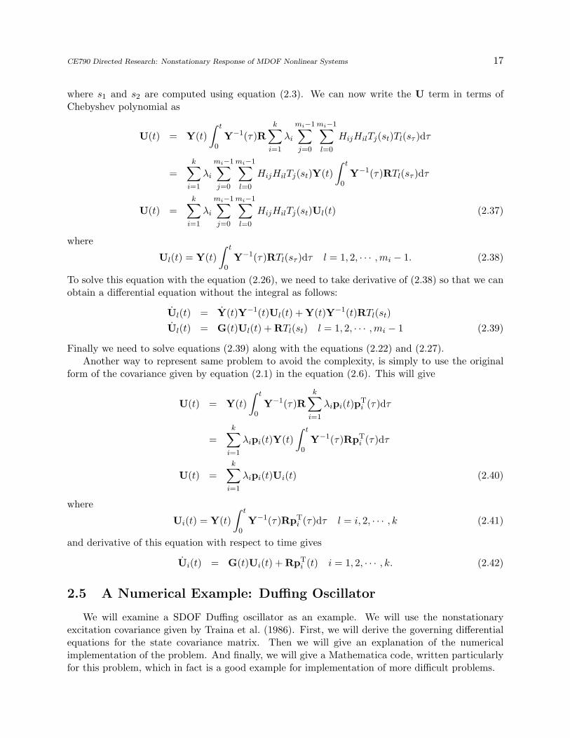
where s1 and s2 are computed using equation (2.3). We can now write the U term in terms ofChebyshev polynomial as

U(t) = Y(t)

∫ t

0Y−1(τ)R

k∑i=1

λi

mi−1∑j=0

mi−1∑l=0

HijHilTj(st)Tl(sτ )dτ

=

k∑i=1

λi

mi−1∑j=0

mi−1∑l=0

HijHilTj(st)Y(t)

∫ t

0Y−1(τ)RTl(sτ )dτ

U(t) =k∑

i=1

λi

mi−1∑j=0

mi−1∑l=0

HijHilTj(st)Ul(t) (2.37)

where

Ul(t) = Y(t)

∫ t

0Y−1(τ)RTl(sτ )dτ l = 1, 2, · · · ,mi − 1. (2.38)

To solve this equation with the equation (2.26), we need to take derivative of (2.38) so that we canobtain a differential equation without the integral as follows:

Ul(t) = Y(t)Y−1(t)Ul(t) +Y(t)Y−1(t)RTl(st)

Ul(t) = G(t)Ul(t) +RTl(st) l = 1, 2, · · · ,mi − 1 (2.39)

Finally we need to solve equations (2.39) along with the equations (2.22) and (2.27).Another way to represent same problem to avoid the complexity, is simply to use the original

form of the covariance given by equation (2.1) in the equation (2.6). This will give

U(t) = Y(t)

∫ t

0Y−1(τ)R

k∑i=1

λipi(t)pTi (τ)dτ

=

k∑i=1

λipi(t)Y(t)

∫ t

0Y−1(τ)RpT

i (τ)dτ

U(t) =

k∑i=1

λipi(t)Ui(t) (2.40)

where

Ui(t) = Y(t)

∫ t

0Y−1(τ)RpT

i (τ)dτ l = i, 2, · · · , k (2.41)

and derivative of this equation with respect to time gives

Ui(t) = G(t)Ui(t) +RpTi (t) i = 1, 2, · · · , k. (2.42)

2.5 A Numerical Example: Duffing Oscillator

We will examine a SDOF Duffing oscillator as an example. We will use the nonstationaryexcitation covariance given by Traina et al. (1986). First, we will derive the governing differentialequations for the state covariance matrix. Then we will give an explanation of the numericalimplementation of the problem. And finally, we will give a Mathematica code, written particularlyfor this problem, which in fact is a good example for implementation of more difficult problems.


2.5.1 Governing Equations for Duffing Oscillator

The nonlinear equations of motion of a simple Duffing oscillator is given by

x(t) + 2ζx(t) + x(t) + λx3(t) = s(t) (2.43)

One should note that for this specific case, M = 1, C = 2ζ, K = 1 and h(x, x) = λq3. Theequivalent linear system is then given by

x(t) + 2ζx(t) + (1 + ke)x(t) = s(t) (2.44)

where

ke = E[∂h

∂x

]= E

[3λx2

]= 3λE

[x2]

(2.45)

and, the state-space form becomes[xx

]=

[0 1

−(1 + 3λE[x2]) 2ζ

] [xx

]+

[0s

]. (2.46)

For this system V is a 2× 2 matrix and V(1, 1) = E[x2]and V(2, 2) = E

[x2]. Therefore, one can

write the equation (2.27) as[X1 X2

X2 X3

]=

[0 1

−(1 + 3λX1) 2ζ

] [X1 X2

X2 X3

]+[0 −(1 + 3λX1)1 2ζ

]+

[X4 X5

X6 X7

]+

[X4 X6

X5 X7

](2.47)

where

X1 = V(1, 1), X2 = V(2, 1) = V(1, 2), X3 = U(1, 1), X4 = U(1, 2),

X5 = U(2, 1), X7 = U(2, 2). (2.48)

Finally we have three nonlinear differential equations:

X1 = 2X2 + 2X4 (2.49a)

X2 = X3 − (1 + 3λX1)X1 − 2ζX2 +X5 +X6 (2.49b)

X3 = −2(1 + 3λX1)X2 − 4ζX3 + 2X7 (2.49c)

One should also note that some of the variables shown here are zeros since

e = 1 ⇒ R =

[0 00 1

]. (2.50)

To be able to solve these equations we need to solve for U, i.e., X4, X5, X6, X7. U is computedfrom (2.37) and (2.39), which includes differential equations also. Therefore we have two groups ofdifferential equations to solve.

Above differential equations are obtained particularly for a Duffing Oscillator. To be aplicabelto a general MDOF system, in the following numerical example we will employ the matrix form ofthe differential equations given by 2.27, (2.41) and (2.42).


2.5.2 Random Excitation and Covariance Kernel

As the covariance excitation, we use the covariance function given by Traina et al. (1986), whichis defined as follows. Consider a random process defined by

x(t) = g(t)Π(t)n(t) (2.51)

whereg(t) = exp (−b1t)− exp (−b2t) and b1, b2 ∈ R (2.52)

Π(t) =

0 : t < 01 : 0 < t < Tm

0 : Tm < t(2.53)

n(t) : N(0,

√2πS0

∆t) (2.54)

where N(m,σ) is Gaussian probability density with mean m and variance σ2. The correspondingcovariance becomes

C(t1, t2) = g(t1)g(t2)Π(t1)Π(t2)Rn(t2 − t1) (2.55)

where Rn(τ) is the autocorrelation function and given by

Rn(τ) =

σ20

[2

3−( τ

∆t

)2+

1

2

(|τ |∆t

)3]

: |τ | < ∆t

σ20

[4

3− 2

|τ |∆t

+( τ

∆t

)2− 1

6

(|τ |δt

)3]

: ∆t 6 |τ | < 2∆t

0 : 2∆t 6 |τ |

(2.56)

where τ = t2 − t1. In this example we take b1 = 1, b2 = 0.1, Tm = 20.1, ∆t = 1 and S0 = 1.

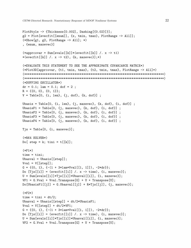
2.5.3 Numerical Solution Technique and Mathematica Source code

It is immediately observed that governing equations are nonlinear differential equations. As an-alytical solution may be difficult to obtain, we solve them numerically. A fourth-order Runge-Kutta(RK4) method is used to solve these equations. We will use the matrix form of the differential equa-tions to illustrate applicability of the method to the MDOF systems. We will use the formulationgiven by (2.41) and (2.42) instead of using the original formulation given in the paper. First we givea very brief summary of the RK4 method. Then we will give the source code that was implementedin Mathemeatica and descriptions of the statements.

Fourth Order Runge-Kutta Method

Consider a set of first order differential equations:

x = f(t, x, y) (2.57a)

y = g(t, x, y). (2.57b)


given the initial values t0, x0 and y0, the values of x and y for the next time step t1 = t0 +∆t arecomputed from

x1 = x0 +∆t

6(k1 + 2k2 + 2k3 + k4) (2.58a)

y1 = y0 +∆t

6(m1 + 2m2 + 2m3 +m4) (2.58b)

where

k1 = f(t0, xn, yn) (2.59a)

m1 = g(t0, xn, yn) (2.59b)

k2 = f(t0 +∆t

2, x0 +

∆t

2k1, y0 +

∆t

2m1) (2.59c)

m2 = g(t0 +∆t

2, x0 +

∆t

2k1, y0 +

∆t

2m1) (2.59d)

k3 = f(t0 +∆t

2, x0 +

∆t

2k2, y0 +

∆t

2m2) (2.59e)

m3 = g(t0 +∆t

2, x0 +

∆t

2k2, y0 +

∆t

2m2) (2.59f)

k4 = f(t0 + (∆t), x0 + (∆t)k3, y0 + (∆t)m3) (2.59g)

m4 = g(t0 + (∆t), x0 + (∆t)k3, y0 + (∆t)m3). (2.59h)

This formulation can easily be extended to system with more than two differential equations, whichis the case for our problem.

In this particular example, we set the time step to 0.1. We used first 20 eigenvalues and 25-order Chebyshev approximation of these eigenvalues. Clearly these values can be modified to obtainbetter approximation of the covariance kernel leading to better results.

Source Code

(*THIS MATHEMATICA FILE COMPUTES THE NONSTATIONARY RESPONSE OF A DUFFING OSC.*)

(*IT USES A FOURTH ORDER RUNGE KUTTA SOLVER TO SOLVE THE DIFFERENTIAL EQUATIONS*)

(*OBTAINED FROM THE LINEARIZATION OF THE SYSTEM*)

Clear["Global‘*"];

(******************************************************************************)

(*COVARINACE FUNCTION (TRAINA ET AL., 1986) *)

covar01[t1_, t2_] := Module[{b1 = 1, b2 = 0.1, Tm = 20.1,

tmax = Tm, dt = 1, S0 = 1,g1, g2, pi1, pi2, tau, sigmasqr, fun1, fun2, Rntau},

tau = t2 - t1;

sigmasqr = 2*Pi*S0/dt;

g1 = Exp[-b1*t1] - Exp[-b2*t1];

g2 = Exp[-b1*t2] - Exp[-b2*t2];

pi1 = If[(0 <= t1) && (t1 <= Tm), 1, 0];


pi2 = If[(0 <= t2) && (t2 <= Tm), 1, 0];

fun1 = sigmasqr*(2/3 - (tau/dt)^2 + 1/2*(Abs[tau]/dt)^3);

fun2 = sigmasqr*(4/3 - 2*Abs[tau]/dt + (tau/dt)^2 - 1/6*(Abs[tau]/dt)^3);

Rntau = If[Abs[tau] < dt, fun1,

If[(dt <= Abs[tau]) && (Abs[tau] < 2*dt), fun2,

If[Abs[tau] >= 2*dt, 0, ERR01]]];

g1*g2*pi1*pi2*Rntau];

(******************************************************************************)

(******************************************************************************)

(*SOME PLOTS OF THE COVARIANCE FUNCTION*)

(*Plot3D[Evaluate[covar01[t1, t2]], {t1, 0, 20}, {t2, 0, 20},

PlotRange -> All]*)

tmax = 20.1; tmin = 0.1; dt = 0.1; t = Range[tmin, tmax, dt]; len = Length[t];

tnew = Table[2*(t[[i]] - tmin)/(tmax - tmin) - 1, {i, 1, len}];

covar = Transpose[Table[Table[covar01[t1, t2], {t1, tmin, tmax, dt}],

{t2, tmin, tmax, dt}]];

(*ListPlot3D[covar,

MeshRange -> {{tmin, tmax}, {tmin, tmax}}, PlotRange -> All]*)

(******************************************************************************)

(******************************************************************************)

(*EIGENVALUES AND EIGENVECTORS OF THE COVARIANCE*)

evals = Eigenvalues[covar];

evecs = Eigenvectors[covar];

(******************************************************************************)

(******************************************************************************)

(*COMPUTATION OF THE CHEBYSHEV POLYNOMIAL APPROXIMATION OF THE COVARIANCE*)

maxevec = 20;

evecfit = Table[0, {i, maxevec}] ;

Do[

tempevec1 = Table[{t[[i]], evecs[[enum, i]]}, {i, 1, len} ];

tempevec2 = Table[{tnew[[i]], evecs[[enum, i]]}, {i, 1, len} ];

NN = 25;

basefun2 = Table[ChebyshevT[i, x], {i, 0, NN}];

evecfit2 = Fit[tempevec2, basefun2, x];

tt = 2*(x - tmin)/(tmax - tmin) - 1;

evecfit[[enum]] = (evecfit2 /. x -> tt);

Block[{$DisplayFunction = Identity}, g1 = ListPlot[tempevec1,

PlotJoined -> True, PlotRange -> All,


PlotStyle -> {Thickness[0.002], Dashing[{0.02}]}];

g2 = Plot[evecfit[[enum]], {x, tmin, tmax}, PlotRange -> All]];

(*Show[g1, g2, PlotRange -> All]; *)

, {enum, maxevec}]

(*apprcovar = Sum[evals[[k]]*(evecfit[[k]] /. x -> t1)

*(evecfit[[k]] /. x -> t2), {k, maxevec}];*)

(*EVALUATE THIS STATEMENT TO SEE THE APPROXIMATE COVARIANCE MATRIX*)

(*Plot3D[apprcovar, {t1, tmin, tmax}, {t2, tmin, tmax}, PlotRange -> All]*)

(******************************************************************************)

(******************************************************************************)

(*DUFFING OSCILLATOR*)

dr = 0.1; lam = 0.1; dof = 2 ;

R = {{0, 0}, {0, 1}};

V = Table[0, {i, len}, {j, dof}, {k, dof}] ;

Ubasis = Table[0, {i, len}, {j, maxevec}, {k, dof}, {i, dof}] ;

UbasisF1 = Table[0, {j, maxevec}, {k, dof}, {i, dof}] ;




Tjs = Table[0, {i, maxevec}];

(*RK4 SOLVER*)

Do[ step = k; tini = t[[k]];

(*F1*)

time = tini;

Ubasval = Ubasis[[step]];

Vval = V[[step]];

G = {{0, 1}, {-(1 + 3*lam*Vval[[1, 1]]), -2*dr}};

Do [Tjs[[i]] = (evecfit[[i]] /. x -> time), {i, maxevec}];

U = Sum[evals[[i]]*Tjs[[i]]*Ubasval[[i]], {i, maxevec}];

VF1 = G.Vval + Vval.Transpose[G] + U + Transpose[U];

Do[UbasisF1[[j]] = G.Ubasval[[j]] + R*Tjs[[j]], {j, maxevec}];

(*F2*)

time = tini + dt/2;

Ubasval = Ubasis[[step]] + dt/2*UbasisF1;

Vval = V[[step]] + dt/2*VF1;

G = {{0, 1}, {-(1 + 3*lam*Vval[[1, 1]]), -2*dr}};






(*F3*)

time = tini + dt/2;

Ubasval = Ubasis[[step]] + dt/2*UbasisF2;

Vval = V[[step]] + dt/2*VF2;

G = {{0, 1}, {-(1 + 3*lam*Vval[[1, 1]]), -2*dr}};





(*F4*)

time = tini + dt;

Ubasval = Ubasis[[step]] + dt*UbasisF3;

Vval = V[[step]] + dt*VF3;

G = {{0, 1}, {-(1 + 3*lam*Vval[[1, 1]]), -2*dr}};





Vnext = V[[step]] + dt/6*(VF1 + VF2 + VF3 + VF4); V[[step + 1]] = Vnext;

Ubasisnext = Ubasis[[step]] + dt/6*(UbasisF1 + UbasisF2 + UbasisF3 + UbasisF4);

Ubasis[[step + 1]] = Ubasisnext;, {k, len - 1}]

(*PLOT THE RESULTS*)

dat = Table[{t[[i]], Sqrt[V[[i, 1, 1]]]}, {i, len}];

ListPlot[dat,PlotRange -> All, PlotStyle -> Thickness[0.01],

PlotLabel -> "Sqrt(E[x1^2])",

TextStyle -> {Helvetica, FontSize -> 12},

AxesLabel -> {"t", ""}, PlotJoined -> True]

dat = Table[{t[[i]], Sqrt[V[[i, 2, 2]]]}, {i, len}];

ListPlot[dat,PlotRange -> All, PlotStyle -> Thickness[0.01],

PlotLabel -> "Sqrt(E[x1^2])",

TextStyle -> {Helvetica, FontSize -> 12},

AxesLabel -> {"t", ""}, PlotJoined -> True]

(******************************************************************************)

2.5.4 Monte-Carlo Simulation and Mathematica Source Code

To investigate the validity of the method and the code, we also carried out a Monte-CarloSimulation. 10000 synthetic excitation is created based on random process definition given above.Then, the Duffing oscillator is analyzed using Runge-Kutta method for a time step ∆t = 0.01.


Source

(*THIS CODE CREATES A SET OF SYNTHETIC EXCITATION AND ANALYZE

THE DUFFING OSCILLATOR FOR EACH OF THE EXCITATION *)

Clear["Global‘*"];

(*******************************************************************)

Needs["Statistics‘ContinuousDistributions‘"];

Needs["Statistics‘DataManipulation‘"];

Needs["Graphics‘Graphics‘"];

(*******************************************************************)

(*******************************************************************)

(* SYSTEM PARAMETERS*)

dt = 1; t0 = 0.1; dt = 1; Tm = 20.1; S0 = 1; sigma0 =

Sqrt[2*Pi*S0/dt]; m = 0;

b1 = 1; b2 = 0.1;

t = Table[i, {i, t0, Tm, dt}]; t = Flatten[{0, t}]; size = Length[t];

newdt = 0.01; newt = Table[i, {i, 0, Tm, newdt}]; newsize = Length[newt];

dr = 0.1; lam = 0.1;

nsim = 3;

sumx = Table[0, {i, 1, newsize}]; sumv = Table[0, {i, 1, newsize}];

(*******************************************************************)

(*******************************************************************)

(* CREATE THE EXCITATION AND ANALYZE THE SYSTEM *)

Do[

dist = NormalDistribution[m, sigma0];

tempn = RandomArray[dist, size];

datn = Table[ {t[[i]], tempn[[i]]}, {i, 1, size}];

datn[[1]] = {0, 0};

interfun = Interpolation[datn, InterpolationOrder -> 1];

interdat = Table[interfun[newt[[i]]], {i, 1, newsize}];

fung = Table[{newt[[i]],

(Exp[-b1*newt[[i]] ] - Exp[-b2*newt[[i]]])}, {i, 1, newsize}];

(*ListPlot[fung, PlotJoined -> True];*)

funn = Table[{newt[[i]], interdat[[i]]}, {i, 1, newsize}];

(*ListPlot[funn, PlotJoined -> True];*)

excit = Table[(Exp[-b1*newt[[i]] ] - Exp[-b2*newt[[i]]])*interdat[[i]], {i,

1, newsize}];

(*ListPlot[Table[{newt[[i]], excit[[i]]}, {i, 1, newsize}],

PlotJoined -> True]*)

(******************************************)

(* RK4 Solution of the duffing Oscillator *)


x = Table[0, {i, 1, newsize}]; v = Table[0, {i, 1, newsize}];

Do [

(*f1 and g1*)

tim = newt[[k]];

disp = x[[k]];

vel = v[[k]];

exc = excit[[k]];

f1 = exc - 2*lam*vel - disp - lam*disp^3;

g1 = vel;

(*f2 and g2*)

tim = newt[[k]] + newdt/2;

disp = x[[k]] + newdt/2*f1;

vel = v[[k]] + newdt/2*g1;

exc = (excit[[k]] + excit[[k + 1]])/2;


g2 = vel;

(*f3 and g3*)

tim = newt[[k]] + newdt/2;

disp = x[[k]] + newdt/2*f2;

vel = v[[k]] + newdt/2*g2;

exc = (excit[[k]] + excit[[k + 1]])/2;


g3 = vel;

(*f4 and g4*)

tim = newt[[k]] + newdt;

disp = x[[k]] + newdt*f3; vel = v[[k]] + newdt*g3;

exc = excit[[k + 1]];


g4 = vel;

v[[k + 1]] = v[[k]] + (newdt/6)*(f1 + 2*f2 + 2*f3 + f4);

x[[k + 1]] = x[[k]] + (newdt/6)*(g1 + 2*g2 + 2*g3 + g4);

, {k, newsize - 1}];

(******************************************)

sumx = sumx + x^2; sumv = sumv + v^2;

(*ListPlot[Table[{newt[[i]], x[[i]]}, {i, 1, newsize}],

PlotJoined -> True];*)

(*ListPlot[Table[{newt[[i]], v[[i]]}, {i, 1, newsize}],

PlotJoined -> True];*)


, {sim, nsim}];

(********************************************************************)

(********************************************************************)

(* PLOT THE RMS VALUES *)

ListPlot[Table[{i, Sqrt[sumx[[i]]/nsim]}, {i, 1, newsize}],

PlotJoined -> True];

ListPlot[Table[{i, Sqrt[sumv[[i]]/nsim]}, {i, 1, newsize}],

PlotJoined -> True];

(********************************************************************)

Save ["c:\montecarlo", "sumv, sumx, newt, newsize, nsim"];

Remarks on Mathematica

Above file was written and compiled in Mathematica Version 4.0.0. The author believes thatMathematica is not the best programming language that can be used to implement this problem.The beneficial part of Mathematica is the function “Fit”, which is very efficient. However, Mathe-matica is not suitable for numerical computation. Its matrix support is very primitive and difficultto understand. Moreover it does not have the capabilities of a standard programming language likeFortran, C or Matlab. It does not have exception handling and debugging capabilities at all, whichmakes the error tracing almost impossible. The author strongly recommends other programminglanguages for this problem. For polynomial fit, Mathematica can be used and, approximated poly-nomial can be transferred to the programming language used. Another problem with Mathematicais that it is not a WYSIWYG (what you see is what you get) program. It is a very high-levelprogramming language (higher that Matlab). The source code that appear on the output (screen)may not be the code that Mathematica kernel processing. The version used is not a stable versionand cause too much trouble with the code and modifies or corrupts it. The author recommends tosave the Mathematica codes into simple ASCII files (“.txt” files) instead of working with originalMathematica files.

2.5.5 Results

Figure (2.2) shows the covariance kernel used. For this covariance, the root mean square dis-placement and the velocity are obtained as shown in figures 2.3(a) and 2.3(b).

As can be from the results, the equivalent linearization method can predict the shape verywell but not the magnitudes. The reason for that is obviously the limited number of eigenvectorsused and low order polynomial approximation. For example, in the original paper, authors use 100eigenvalues and 200-order approximation. Also, the a smaller time step should be chosen for theRK4 solution. Another possibility is an error in the source code. The code should also be reviewedand should be executed in more stable versions of Mathematica.

One suggestion is to work on the polynomial fit separately to obtain a better approximation ofthe covariance kernel. After that the RK4 solver can be improved for better results.

Although, looks complex, the author believes that this method is quite straightforward and staysas a powerful tool for the analysis of the nonlinear structures excited by nonstationary excitation.


2.5.6 Conclusion

In this section, we reviewed the method proposed by Smyth and Masri (2002) for the analysisof nonlinear MDOF systems excited by nonstationary excitation. A Mathematica code is presentedfor the analysis of a Duffing oscillator. The results of the method is compared with a Monte-Carlosimulation. Suggestions for the improvement of the method are given.

5

10

15

20

5

10

15

20

0

0.5

1

1.5

2

5

10

15

Figure 2.2: Covariance kernel of the excitation

5 10 15 20t

0.25

0.5

0.75

1

1.25

1.5

(a) Displacement

5 10 15 20t

0.25

0.5

0.75

1

1.25

1.5

1.75

(b) Velocity

Figure 2.3: Root mean square values of the responses (Dash: Monte-Carlo Simulation, Solid:Equivalent Linearization)

Bibliography

Kazakov, I. E. (1965). “Generalization of the method of statistical linearization to multidimensionalsystems.” Automatic Remote Control, 26, 1201–1206.

Meirovitch, L. (1986). Elements of Vibration Analysis. McGraw-Hill, New York, second edition.

Papoulis, A. (1984). Probability, Random Variables and Stochastic Processes. McGraw-Hill, NewYork, second edition.

Reid, J. G. (1983). Linear System Fundamentals: Continuous and Discrete, Classic and Modern.McGraw Hill, New York.

Roberts, J. B. and Spanos, P. D. (1990). Random Vibrations and Statistical Linearization. JohnWiley & Sons, New Jersey.

Smyth, A. W. and Masri, S. F. (2002). “Nonstationary response of nonlinear systems using equiv-alent linearization with a compact analytical form of the excitation process.” Probabilistic Engi-neering Mechanics, 17(1), 97–108.

Stark, H. and Woods, J. W. (2002). Probability and Random Processes with Applications to SignalProcessing. Prentice-Hall, New Jersey, third edition.

Traina, M. I., Miller, R. K., and Masri, S. F. (1986). “Orthogonal decomposition and transmissionof nonstationary random process.” Probabilistic Engineering Mechanics, 1(3), 136–149.

Wirsching, P. H., Paez, T. L., and Ortiz, K. (1995). Random Vibrations. John Wiley & Sons, NewYork.

28

CE790 Directed Research A Report on Nonstationary...

Documents

Transcript of CE790 Directed Research A Report on Nonstationary...