1

COLLEGE OF

ENGINEERING Department of Civil & Geological Engineering

CE 463.3 – Advanced Structural Analysis

Compilation of All 2013 Labs Using SAP2000

T.A: Ouafi Saha Professor: M. Boulfiza

Overview Objectives:

• Give an over view of the basic commands of SAP2000 • Use of SAP2000 to solve various structural problems • Develop the ability to continue a self-learning process • Check and solve assignment questions

1. Introduction to Computation Modeling in Engineering:

Engineering process from Conceptual idea to Fabrication (The Finite Element Method – A Practical Course. by G.R. Liu, S.S. Quek)

Conceptual Design

Modeling Physical, Mathematical, Computational

Operational and Economical

Simulation Experimental, Analytical and Computational

Analysis Listing, Photography,

Computer graphics and Virtual reality

Design

Prototyping

Testing

Fabrication

2

2. Computation Hardware tool:

Simplified scheme for Computer 3. Computation Software tool:

Simplified scheme of a computer software 4. SAP2000: SAP2000 is a program based on The Finite Element Method (FEM). It is one of a long list of software packages having the FEM as their kernel. A non-exhaustive list is available at this address: http://en.wikipedia.org/wiki/List_of_finite_element_software_packages The program is edited by a company named CSI (Computer and Structure Inc.) founded in 1975. The very first version of SAP was SAP, followed later by SOLIDSAP and SAP IV. With the development of PC computers, SAP was released in two major versions SAP80 and SAP90. Basically these two versions and the previous ones were based on TEXT files for both input and output. In 1996 the first version of SAP2000 was released, it had an integrated graphical user interface working completely under Microsoft Windows. The choice of SAP2000 in this course is mainly due to its civil engineering orientation and to its relative ease of use. SAP2000 has an integrated graphical user interface similar to some older versions of Autocad’s interface. Various documents and tutorials are available:

• Built-in help and PDF documentation. • http://www.csiberkeley.com/sap2000/watch-and-learn • A search in google or youtube with keywords “sap2000 tutorial” leads to plenty of documents

and videos, but try to start with the easiest ones.

Input

Central Unit

Output

Pre-Processor Import, Interactive

Processor Interpretation of data, Detection of Errors, Formation of Sys. Eq., Solve Sys., Iteration

Post-Processor Visualization, Design

3

5. Basic Steps to Solve a Structural Problem using SAP2000: 1. Start-up by choosing units, setting up grids or by choosing a model from the library 2. Define materials, element properties, loading patterns, analysis cases and combinations 3. Draw the model using the powerful graphical interface and selection and editing tools 4. Assign displacement boundary conditions (supports) 5. Assign loads (forces, moments, displacements, pressure, temperature…) 6. SOLVE system, use simplification if possible 7. Display Output in graphical and/or tabular form 8. Analyze results

6. List of the Labs:

Lab 1 – Simple Beams and Frames .......................................................................................... 4 Lab 2 – Truss Structures ........................................................................................................ 14 Lab 3 – Elaborated Beam and Frame Structures .................................................................... 19 Lab 4 – SAP2000 Plane Elasticity ......................................................................................... 25 Lab 5 – Dynamic Analysis ..................................................................................................... 39 Lab 6 – Geometric Nonlinearity and P-Δ effect .................................................................... 53 Supplemental Material for SAP2000 – Convention used ...................................................... 58

4

Lab 1 – Simple Beams and Frames 1. Simply supported beam http://www.youtube.com/watch?v=IrYnpP2vDp0

Units kN, m, C Material Concrete, Section 30x50cm2, each segment is 1.5m, Two possible ways to model it Steps: Start SAP2000 by using: internet explorer pointing at the url address http://www.engr.usask.ca/vdi/ or http://www.engr.usask.ca/engr-apps/ , you can also save the link to your desktop and execute it. Login using your nsid. Choose New model > select appropriate units and click on grid only

In the next dialog box enter the appropriate values

5

Close 3D window and choose view for the 2D view Select Define > Section Porpertires > Frame Sections… then click on Add New Properties

Select Concrete and Rectangular section

6

Name the section Beam and enter 0.5 as Depth and 0.3 as Width Click on Ok twice Draw the Beam as five consecutive elements, starting from the origin to each next key point, make sure the section in the flying box is Beam. End drawing by esc or double click.

Select Node B, Assign > Joint > Restraints… then select

Select Node F, Assign > Joint > Restraints… then select Try a quick run and see how to neglect self-weight http://www.youtube.com/watch?v=xajE-OhAut8 Select Element A-B, Assign > Frame Loads > Distributed… enter 15 under Uniform Load Select Element B-C, Assign > Frame Loads > Distributed… enter 15 under Uniform Load

7

Select Node D, Assign > Joint Loads > Forces… enter -45 in Force Global Z Select Node E, Assign > Joint Loads > Forces… enter -22.5 in Force Global Z

Before Solving, take a look at the final configuration, and particularly loading Menu Display > Show Load Assigns > Frame/Cable/Tendon… The screen should show a beam like the following

Our beam can be treated in two dimensions as a 3 DOF system. This can considerably reduce the size of the problem for a very fine mesh (high number of elements and nodes). Menu Analyze > Set Analysis Options… Click on Plane Frame You can see that the only active DOF’s available are the two translations X and Z and one rotation RY.

8

Now we can run the Analysis or F5 or Menu > Analysis > Run Analysis…

Make sure to turn off the analysis of Modal Case Click on Run Now You will be prompted to save your work if it has not been done yet. It is recommended to save your work on a regular basis. Now, it is time to analyze our results and decide if they are acceptable or need to be reviewed in some way. Check deformed shape, Support reactions Internal forces and moments

9

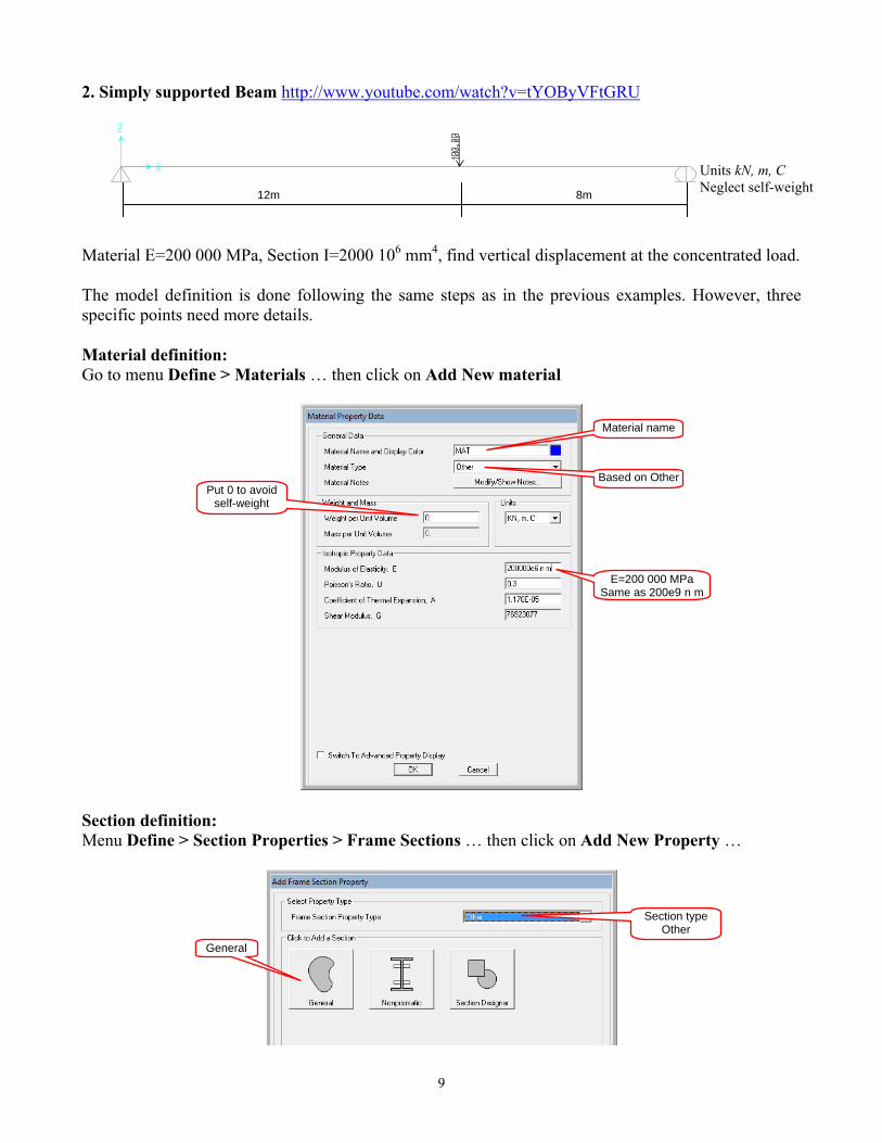
2. Simply supported Beam http://www.youtube.com/watch?v=tYOByVFtGRU

Material E=200 000 MPa, Section I=2000 106 mm4, find vertical displacement at the concentrated load. The model definition is done following the same steps as in the previous examples. However, three specific points need more details. Material definition: Go to menu Define > Materials … then click on Add New material

Section definition: Menu Define > Section Properties > Frame Sections … then click on Add New Property …

12m 8m

Material name

Based on Other Put 0 to avoid

self-weight

E=200 000 MPa Same as 200e9 n m

Section type Other

General

Units kN, m, C Neglect self-weight

10

Make sure your beam has the section SEC defined above and that this section is made of the particular material MAT. Make sure to not include self-weight as well by putting material weight = 0. Neglect self-weight Menu Define > Load Patterns …

Change Self Weight Multiplier to 0 in the DEAD load pattern and click on Modify Load Pattern, then OK.

All values can be 0 except

I33=2000 106 mm4

Select Material MAT defined in previous step

Change default name FSEC1 to your preferred

11

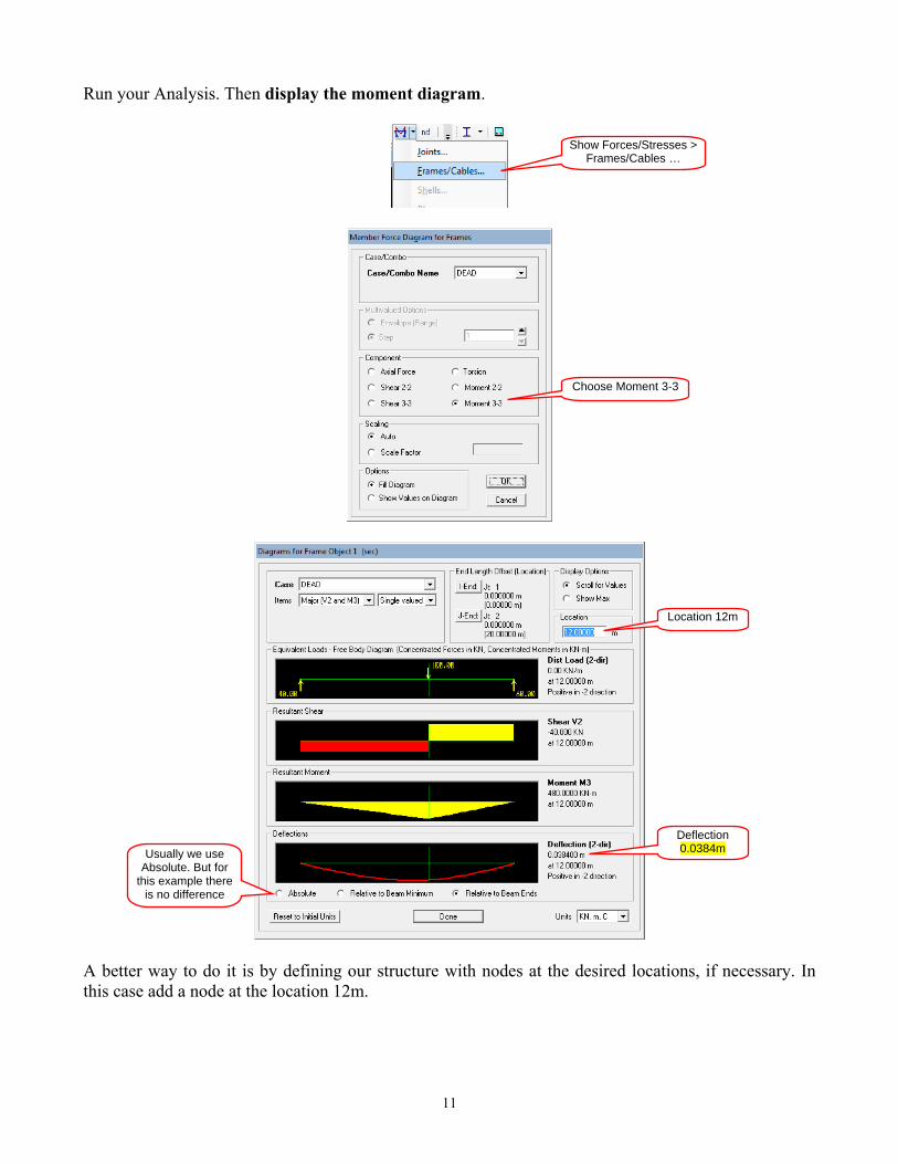
Run your Analysis. Then display the moment diagram.

A better way to do it is by defining our structure with nodes at the desired locations, if necessary. In this case add a node at the location 12m.

Show Forces/Stresses > Frames/Cables …

Choose Moment 3-3

Location 12m

Usually we use Absolute. But for

this example there is no difference

Deflection 0.0384m

12

3. Simply loaded Frame

At least two ways to define our structure are possible; with and without a node at point C. The steps to define the structure are almost the same as in the previous examples. Unit and Grid; Material and Section (don’t forget to add the cross section A); Draw the structure either with a step at point C or without; Support and Loads; Analysis of Plan Frame. For the horizontal displacement at point A click on the Show Deformed Shape button then put the mouse pointer close to the point A, a bubble appears showing information about that point, the horizontal displacement parallel to X axis is U1 = -0.008 (in this case in the opposite X direction) because local and global axis have the same orientation for the nodes. You can also right click on the node to see these values more precisely in a box. These values are given relatively to the undeformed shape.

Point A (U1=Ux=-0.008, U2=Uy=0, U3=Uz=-0.09117, R1=Rx=0, R2=Ry=0.012, R3= Rz=0) Displacements are given in the distance Unit, Rotations are given in radian according to the right hand rule. With a node at C We can use the grid system X (0, 4, 8) and Z (0, 2, 4). We are not using the Y axis so fare. The steps to find the vertical displacement at point C are the same as those for point A, the only difference is to look for U3 = -0.04317 in the negative Z direction.

4m 4m

2m

4m

Material E=200 000 MPa Geometrie I = 500 106 mm4

A = 2000 mm2

C

A

13

Without a node at C We can use the grid system X (0, 8) and Z (0, 2, 4). In this case we do not have a node at point C and the determination of the vertical displacement is done by displaying the information of the horizontal element (8m beam). For this purpose show the moment 3-3 diagram.

Then right click on the horizontal element. To show the detailed results

If you get a little difference with the hand calculated values try to explain why.

Select mid-span

Select Absolute to get vertical displacement

with respect to the global axis (XYZ) Note: positive in -2

direction

14

Lab 2 – Truss Structures

1. Simple Truss Structure http://www.youtube.com/watch?v=lHS17C5Ntf8

New features: Edit Coordinate Systems/Grids The same steps:

• Units (kN, m, C) Grids X (0,2,5), Y(0), Z (0, 2) Choose XZ view

• Define Materials: we need only E=200 GPa, Element properties: we need only A = 10 cm2

Many ways to do the analysis of Truss structures. The easiest way is to put all other geometric properties = 0 except the Cross Sectional (axial) Area.

• Draw the model • Assign Supports • Assign one concentrated load at point P

To avoid having warnings in the solver module, keep only UX and UZ DOF in the Analysis Options

3m 2m

P = 15 kN

E = 200 000 MPa A = 10 cm2

Neglect self-weight What is the vertical displacement at P? 2m

Only Cross section different from 0

15

• SOLVE • Display Output Displacement and forces • Analyze results

Deformed shape

We can have the displacement of any node (joint) by right clicking on it.

The vertical displacement of point P is then U3 = -5.784 10-4 m

Internal forces In this case, only the Axial Forces are present

Keep only UX and UZ. No rotation

16

2. Elaborated Truss structure http://www.youtube.com/watch?v=VqqJnpFxDIM The Top and Bottom chord section is double angle 2L5x5x7/16 The Braces section is rectangular 7x25 mm2 New features: Import sections, Edit Divide, Releases - Run three analyses, perfect welding in all joints, hinges in all joints, only braces are hinged. - Compare the three cases - What is the maximum deflexion in each case? - What are the maximum internal forces in these cases? Follow the same eight steps. Use the following grid specification: X (-9, 0, 9), Y (0), Z (0, 4). The new features are explained below.

• Import section To use a section profile from the SAP2000 database, go to Define > Section Properties > Frame Sections … then click on Import New Property …

Select the type of the section profile “Double Angle” and the path for the section database should be C:\Program Files (x86)\Computers and Structures\SAP2000 15 Then select “SECTIONS8.PRO” file.

Units kN, m, C Mat. Steel Self-Weight = 0

4 m

25kN

3 m 3 m 3 m 3 m 3 m

25kN 25kN

25kN

30kN

3 m

17

Finally, select the appropriate section from the list; “2L5x5x7/16” in this case.

• Edit divide option Select the four elements, two lower chords and two upper chords, and divide them into 3 segments each. Edit > Edit Lines > Divide Frames …

• Releasing the hinged elements Select elements, Assign > Frame > Releases/Partial Fixity …

SECTIONS8.PRO common Profile DBLocal Disk C:

Path: C:\Program Files (x86)\Computers and Structures\

SAP2000 15

18

3. Additional Examples

50.0

0

Find internal forces and the deflection at the applied load point. Another detailed Truss example http://www.ce.memphis.edu/7111/projects/SAP_2000/SAP_2000_trusses.html

4 m4 m

2 m

2 m

Units kN, m, C Self-Weight = 0 E = 200 GPa A = 1500 mm2

19

Lab 3 – Elaborated Beam and Frame Structures 1. Continuous Beam http://www.youtube.com/watch?v=skScVFEefRw

New features: Elaborated Loads, Local Axis Load pattern possibilities The most used, but not the only possibility, is the distributed load over frame elements. You can access it by selecting the frame element, then Menu Assign > Frame Loads > Distributed …

Local axes rotation For the local axis convention refer to the supplementary document, available on the class web site. The angular unit in SAP2000 is the degree. Let’s try to rotate the right end support by 30° counter clockwise. Select the extreme right node, Menu Assign > Joints > Local Axis …

Select Load Name Other Possibility for Unit conv

Force or Moment?

Coordinate System and Direction

Up to four definition points for the load

Make sure to select the right option

To used in case of uniform load over the whole frame element

At relative or absolute distance from node i

Value of the load

Possible way of combination

Units t, m, C Mat. Concrete Self Weight = 0

20

Displacement loading. Try to find and explore. In which kind of situation should we use it? Questions: - What are the extreme vertical deflections of the beam? - What are the reactions at each support? - Plot the internal forces and moment diagrams. - What about the axial force after support rotation? 2. Simple Frame with enhanced loading and different cross sections http://www.youtube.com/watch?v=Z1R0hE9RdkA

New features: Sections, Display, Local Axes Visualisation Section possibilities For the Tee section go to Menu Define > Section Properties > Frame Sections … Click on Add New Property… then Select type Steel and section Tee For Dimensions Name Convention refer to the supplementary document (available on the class web site).

3 t/m

2 t/m 6 t.m

60

55

15 125

25

25

5t

4t

4t

3.0

4.0

6.0 5.0 3.0

1.5 1.5 2.5

l/2

l/2

Why -30?

P

Units t, m, C Mat. Concrete Self Weight = 0

Sections in cm

21

Axis Visualization and Extruded View To change the visualisation default options, use Menu View, Set Display Options (Ctrl+E) Check Frame/Cables/Tendons Local Axes and Extrude View.

Questions: - What values, distances, and directions should we use for the two intermediate concentrated loads? Check supplementary document. - Extract all results for point P (Displacement and internal forces). - Plot internal forces diagrams (N, T, and M) - What would happen if we forget to modify the concrete material? 3. Load Combination (ref. CE321)

New features: Load Combination, Output stations, Tabular Output.

Name

Material, 4000 Psi for

Concrete

Quick preview of the Section

t3 =70 cm t2 =125 cm tf =15 cm tw =25 cm

5 m 2.5m

Units kN, m, C Material Concrete Section 300x650mm2

Self-Weight included in Dead Load

Live Load = L2 = 15 kN/m

Live Load = L1 = 15 kN/m

Dead Load = WD = 10 kN/m and PD = 60kN

PD WD

22

Load Combination Use Menu Define with Load Patterns, Load Cases, and Load Combinations commands.

We define first three load patterns D, L1, L2 as linear static. When assigning the loads, make sure to assign them to the appropriate load pattern. Define the load combinations. Consider the following combinations: 1.4 D 1.25 D + 1.5 L1 1.25 D + 1.5 L2 1.25 D + 1.5 (L1 + L2) 0.9 D + 1.5 L1 0.9 D + 1.5 L2 0.9 D + 1.5 (L1 + L2) Output stations By default SAP2000 uses 1 intermediate point (on top of the two end nodes) to show internal forces. When this is not sufficient, it is recommended to use more intermediate points. Five to nine output stations seems to be reasonable. Select the elements for which you want to modify the output station, and go to Menu Assign > Frame > Output Stations…

Tabular Output Graphic output is very friendly and useful, but sometimes difficult to analyse or to visualise. An exhaustive listing of the input and/or output is in these cases inevitable. To see the structure parameters in tabular form use Menu Display > Show Tables… or Ctrl + T There are many functionalities to explore.

23

Questions - Which one, of the previous combinations, gives the Maximum Positive Moment and which one gives the Maximum Negative Moment? - Why is it important to consider the combination 0.9 D since it is smaller than 1.25 D? - Plot the linear envelope for these seven combinations. 4. Multi Story Building

7 m5 m6 m6 m

4 m3 m

3 m

New features: Modify Grid, Editing, Selection

Units kN, m, C Mat. Steel Self Weight = 0 Beam S10x35 Column1 W10x45 Column2 W10x15

24

Choose 2D Frames from the new model. Enter portal Frame Dimensions as shown below.

For Section Properties click on button to access the sections dialogue box. Click on Import New Property… then select material steel and click on I / Wide Flange. Then Select S10x35 for beams and select W10x45 for columns. Modify Grid according to our example Menu Define > Coordinate Systems/Grids… click on Modify/Show System… Change Values for coordinates X and Z Grid Data as required such as X (-12,-6,0,5,12) and Z (0,4,7,10) and check Glue to Grid Lines box.

Another way to reach the same result is to use Menu Edit > Move and/or Replicate Selection - Selection of the basement nodes (difference between right and left) - Selection by Element Properties - Selection by Coordinate Specification Questions: - Find the position and the value of the Maximum Base Reactions. - Find the position and the value of the Maximum horizontal displacement. - What change would you suggest for the structure to be more balanced? - Do the same Analysis assuming the horizontal forces multiplied by two. Is it possible to implement the change in a single action?

25

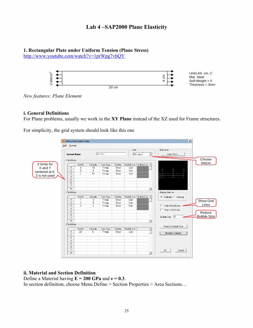
Lab 4 –SAP2000 Plane Elasticity 1. Rectangular Plate under Uniform Tension (Plane Stress) http://www.youtube.com/watch?v=1prWpg7vhQY New features: Plane Element i. General Definitions For Plane problems, usually we work in the XY Plane instead of the XZ used for Frame structures. For simplicity, the grid system should look like this one

ii. Material and Section Definition Define a Material having E = 200 GPa and v = 0.3. In section definition, choose Menu Define > Section Properties > Area Sections…

Units kN, cm, C Mat. Steel Self-Weight = 0 Thickness = 3mm

20 cm

4 cm

2 kN

/cm

2

Show Grid Lines

Reduce Bubble Size

3 Grids for X and Y

centered at 0. Z is not used

Choose kN/cm

26

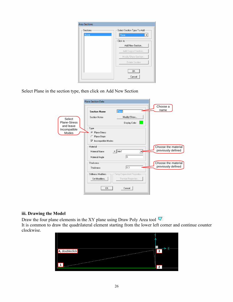
Select Plane in the section type, then click on Add New Section

iii. Drawing the Model Draw the four plane elements in the XY plane using Draw Poly Area tool It is common to draw the quadrilateral element starting from the lower left corner and continue counter clockwise.

Choose a name

Choose the material previously defined

Choose the material previously defined

Select Plane-Stress

and leave Incompatible

Modes

2

3 4, doubleclick

1

27

We need a finer mesh, to have more accurate results. Select the four elements and go to Menu Edit > Edit Areas > Divide Areas…

Some recommendations are given in the reference manual about the aspect ratio of the elements. One should follow them to get the most accurate results. iv. Displacement Boundary Conditions Even if there are no apparent supports in the initial problem, we must specify some restraint conditions for the program to avoid a singular stiffness matrix. In this case, due to geometric and loading symmetry, we know that the central node will not move in either X nor Y direction. Also, all nodes on the Y axis will not move in the X direction. Select all nodes on the Y axis and specify Translation Restraints in direction 1, then select the node at the origin and specify Translation Restraints in both Directions, 1 and 2

v. Loading Condition Two possible ways exist for applying the loads; by loading the nodes or by loading the elements. Nodes (joints) For the right side, the total load is F = (2 kN/cm2) x (4 cm) x (0.3 cm) = 2.4 kN in the +X direction. We also have 5 nodes, 3 medians and 2 corners. The load distribution will be as follow: For median nodes f = 2.4 / 4 = 0.6 kN. For corner nodes f = 0.6 / 2 = 0.3 kN. By symmetry, the same loads are applied to the left side.

Divide each element into 4 by 2 elements according to convention (supplemental)

28

Element (Area) For the right side, we have a uniform pressure in the outward direction. Select the four right edge elements > Assign > Area Loads > Surface Pressure (All)…

For the left side, we only change face 2 by face 4.

vi. Analyse the System In plane elasticity problems, only two displacements are considered. Menu Analyze > Set Analysis Options …

Then Run the analysis. Remember to save your work, to neglect self-weight and to disable modal analysis.

-2, negative pressure (outward direction)

Face 2 (Supplemental doc)

29

vii. Display Output We can see the deformed shape as:

And the internal stresses (S11) as

viii. Discussing Results As we may have expected we can say:

- In the displacement diagram, the effect of positive Poisson’s ratio is clearly seen. - In the stress diagram, we have uniformly distributed longitudinal horizontal stresses over the

whole solid. Neither shear stresses nor longitudinal vertical stresses exist in the solid. 2. Tension Connection plate http://www.youtube.com/watch?v=uvmdgD6aU0M New features: Pipe and Plate Module Only half of the structure will be modeled. As SAP2000 is not extremely powerful in 2D and 3D modeling, the structure will be drawn using three elemental parts. Start a blank file with only grids. X(0,5,15,25), Y(-10,0,10), Z(0) Set Auto-merge tolerance to 0.1 mm, Menu Option > Dimensions/Tolerances…

Symmetry

15 mm

R=10mm

r = 5mm

F=0.1 kNF=0.1 kN Units kN, mm, C Mat. Steel Self-Weight = 0 Thickness = 2 mm

Set auto merge to 0.1mm or you will

have a strange mesh

30

- Start with rounded plate with circular hole

Menu Edit > Add Model From Template … then click on Pipes and Plates

The main parameters are highlighted.

We need to delete the left half part of the circle, and reduce the number of nodes. For this purpose it is better to leave only one slice of the model, merge all the elements then divide them into 4 elements in the vertical direction. The final step is replicating the slice to reproduce the final form.

31

Select all elements in the previous screen and apply Replicate commad, from the Edit Menu. Make sure to enter the parameters as in the figure below. Save your file from time to time!

32

- Rectangular plate with circular hole Menu Edit > Add Model From Template … then click on Pipes and Plates

We should remove the right half side of the rectangular plate and move the remaining part 15mm in the X direction (right), using the Move command from the Edit Menu.

33

- Last Rectangular part We draw a big rectangle and divide it into 4 parts in X direction and 16 parts in Y Direction.

The final model should look like the figure above. Due to Symmetry, the same boundary conditions as in the first example will be applied here as well. One concentrated nodal load will be applied to the node at coordinate (20, 0) F = 0.1kN in X direction. For the analysis we will only consider displacements in the X and Y directions. Run the Analysis

34

Output Time for some nice pictures

Deformed shape (effect of concentrated Load) Resultant Displacement Contour Lines

The three stress components in the local axis and the Von Mises stress.

35

3. Import 2D models http://www.youtube.com/watch?v=vrSO462W39U Another efficient way to model two dimensional and three dimensional structural problems is to use the import functionality of SAP2000. Many formats are supported by the program, but the data must be prepared in a strict form. The same Problem 2 will be done using .DXF import function. It is possible to use a simple modeling software such as Automesh2D, freely available from the website http://www.automesh2d.com/default.htm.

The geometric file used by this software is a text file containing the following data

1 2 4 1 0 -10 0 2 25 -10 10 3 25 10 10 4 0 10 0 6 1 10 0 0 2 10 5 5 3 20 5 5 4 20 -5 5 5 10 -5 5 6 10 0 0

36

The next step is to mesh the structure using the easiest auto-mesh function. 250 elements are chosen.

The final step in this software is to export the meshed structure in dxf format. Before importing the model into SAP2000, it is usually recommended to edit the mesh in Autocad and copy all lines in a specific layer. This layer will be used by SAP2000 to import the appropriate model. In SAP2000, use Menu File > Import > Autocad .dxf File … the select your file.

Select upward direction Select from which layer import which elements

37

The next step is to draw a Plane element enclosing the whole imported model. Remember we imported the model as frame elements, but we need Plane element.

The final step is to divide the big plate element into the shape of the little frame lines. Select all and Menu Edit > Edit Areas > Divide Areas …

Delete the unwanted plane parts, the central circle and the two big corners. Delete also the frame elements as they don’t belong to our desired model. Done! At least for the geometry modeling part. See video for more details. 4. Additional Examples 4.1. Plane Stress Repeat Problem 1, add a uniformly distributed load = 1 kN/cm2 in compression at the top and bottom faces of the plate. 4.2. Cantilever Beam (Thick theory) Follow the same steps as Problem 1, take care about unit conversion. The load is uniformly distributed over the length, must be converted to node concentrated forces or uniformly distributed pressure. - Compare this solution with your classic beam analysis. Check deflection and maximum stress.

Units kN, m, C Mat. Steel Self-Weight = 0 Thickness = 7.5mm

2.0 m

3kN/m

0.2 m

38

4.3. Bracket Compare the solution of the given example Bracket.SDB with the one given by Ansys. The web link is a pointer to the University of Alberta tutorial for Ansys. http://www.mece.ualberta.ca/tutorials/ansys/BT/Bracket/Bracket.html

The Model under SAP2000 3D model from the U of A website

39

Lab 5 – Dynamic Analysis 1. Natural Mode for a Single Degree of Freedom system http://www.youtube.com/watch?v=HTOt2uJgdRg Let’s start with a simple single degree of freedom system composed of a column fixed at its base and a concentrated mass at its top. We need to know the natural frequency and period of this structure. M = 20 000 kg E = 200 GPa I = 100 106 mm4 h = 3m

( ) ( )( ) ( )

3 3

3 9 2 6 4

20000 32 2 2 0.596sec

3 / 3 200.10 / 100.10

kg mm mTk EI h N m m

π π π−

×= = = =

× ×

i. General Definitions It is HIGHLY recommended to choose (N, m) as principal units so mass will be in kg. Otherwise, conversion will not be obvious. Version 14 of SAP2000 allows you to enter mass as weight, this may simplify data input, but you must be careful on the meaning of each possibility. A simple grid system may be X(0), Y(0), Z(0,3) ii. Material and Section Definition Define a Material having E = 200 GPa and v = 0.3. Also, define a frame section having moment of inertia I3=100.106mm4. Make sure to choose the appropriate Material for this section. iii. Drawing the Model Draw a frame from point p1(0,0,0) to p2(0,0,3). iv. Boundary Displacement Conditions Assign a fixed restraint to the base of our element. v. Loading Condition Since we are just looking for the dynamic properties of our structure we don’t need a loading condition, but we need to assign a concentrated mass to the top of our column. Select the top node (joint) Assign > Joints > masses …

M

40

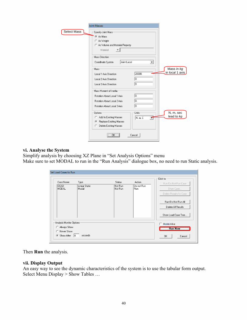
vi. Analyse the System Simplify analysis by choosing XZ Plane in “Set Analysis Options” menu Make sure to set MODAL to run in the “Run Analysis” dialogue box, no need to run Static analysis.

Then Run the analysis. vii. Display Output An easy way to see the dynamic characteristics of the system is to use the tabular form output. Select Menu Display > Show Tables …

Mass in kg in local 1 axis

Select Mass

N, m, sec lead to kg

41

viii. Discussing Results As we can see, the same period T = 0.596075sec as the hand calculated one is obtained. The natural frequency is f = 1.6776 Hz and the circular frequency is ω = 10.541 rad/sec

42

2. Natural Mode for a Single Degree of Freedom one storey Building http://www.youtube.com/watch?v=O1rZRojOf4c Let’s study the structure shown in the next figure. Assumptions: - Structure works in XZ plane. - All members are made of steel, E=200GPa. - All members’ self-weight is neglected. - The only existing mass is concentrated in the roof. - Structure is fixed at its base. Columns W310x74 (from CISC data base) Ic = 165.106mm4 h = 3m, l = 6m, M = 30 000kg. Roof will be modeled in four different ways. Quick steps: - Choose N, m, C units - Define grids X(0,3,6) Y(0) Z(0,3) - Add new material Mat (E=200E9, v = 0.3, Self-weight=0) - Add section W310x74 by importing I/Wide flange from CISC database - Draw the frame using the same section for all parts - Fix foundation - Draw Special Joint at the middle of the roof

- Assign concentrated mass to that joint = 30000 in local 1st direction as mass. (§ expl. 1) - Only planar XZ degrees of Freedom are needed for this problem - No need for static analysis

M

E, Ic hE, Ic h

E, Ib l

43

a. Roof as Normal beam Just like we have already defined our structure In this case Ib = Ic The roof is very flexible. T = 0.284162 sec f = 3.5191 Hz b. Use of Diaphragm Select all three top nodes then go to Menu Assign > Joints > Constraints … Select diaphragm in the first dialogue box and keep Z axis selected in the second dialogue box. This enforces the selected joints to maintain exactly the same distance from each other while moving in the XY plane.

This constraint is usually used to model concrete slabs or decks. This does not lead to a big change in the example under consideration. The reason is that only the compression in the roof beam has been constrained. T = 0.28251 sec f = 3.5397 Hz Alternatively, we can use the Equal Constraint. In this case choose all DOF to be equal. As we see from the figure, the structure is stiffer but this condition is not realistic. T = 0.243478 sec f = 4.1071 Hz

44

c. Increase the stiffness of the roof beam Remember to remove constraints before doing this step. Select the top beam then Menu Assign > Frame > Property Modifiers …

In this case we are multiplying the flexural stiffness (Moment of Inertia I3) of the top beam by a factor of 10. It’s clear that the top slab is almost horizontal. T = 0.234911 sec f = 4.2569 Hz d. No rotation in the top beam Remember to set the property modifiers to 1 again. Select the three nodes of the top and Assign > Joints > Restrains …

This is the closest “realistic” condition to the use

of the formula 312

hEIk = for column stiffness.

T = 0.219775 sec f = 4.5501 Hz Why do you thik the above result is different from yours? Theoretical period calculated with formula above is T=0.2009sec. How can you find it with SAP2000?

45

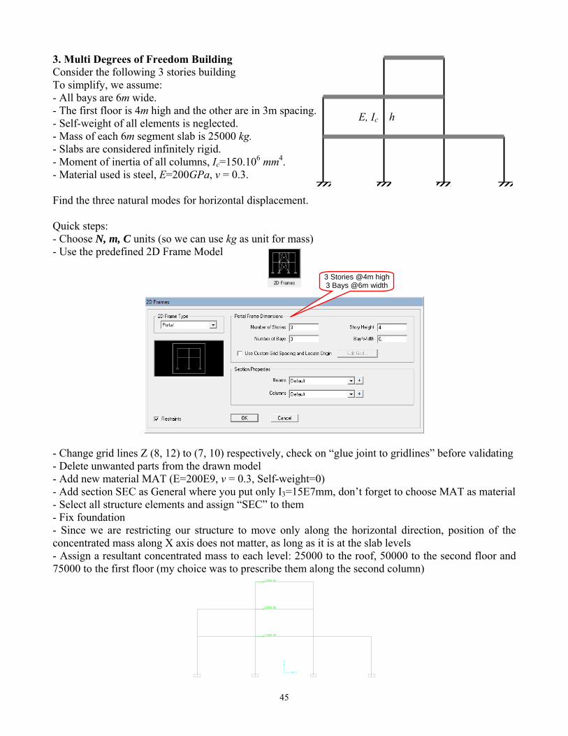
3. Multi Degrees of Freedom Building Consider the following 3 stories building To simplify, we assume: - All bays are 6m wide. - The first floor is 4m high and the other are in 3m spacing. - Self-weight of all elements is neglected. - Mass of each 6m segment slab is 25000 kg. - Slabs are considered infinitely rigid. - Moment of inertia of all columns, Ic=150.106 mm4. - Material used is steel, E=200GPa, v = 0.3. Find the three natural modes for horizontal displacement. Quick steps: - Choose N, m, C units (so we can use kg as unit for mass) - Use the predefined 2D Frame Model

- Change grid lines Z (8, 12) to (7, 10) respectively, check on “glue joint to gridlines” before validating - Delete unwanted parts from the drawn model - Add new material MAT (E=200E9, v = 0.3, Self-weight=0) - Add section SEC as General where you put only I3=15E7mm, don’t forget to choose MAT as material - Select all structure elements and assign “SEC” to them - Fix foundation - Since we are restricting our structure to move only along the horizontal direction, position of the concentrated mass along X axis does not matter, as long as it is at the slab levels - Assign a resultant concentrated mass to each level: 25000 to the roof, 50000 to the second floor and 75000 to the first floor (my choice was to prescribe them along the second column)

E, Ic h

3 Stories @4m high3 Bays @6m width

46

- Select all nodes above foundation and assign horizontal diaphragms to each level

- Select all nodes above foundation and assign restrained rotation about local 2nd axis - Only planar XZ degrees of Freedom are needed for this problem - Run the analysis with No static analysis

T1=0.56032sec, T2=0.20508sec, T3=0.13491sec and f1=1.785Hz, f2=4.876Hz, f3=7.412Hz

Horizontal Diaphragm

Each level

47

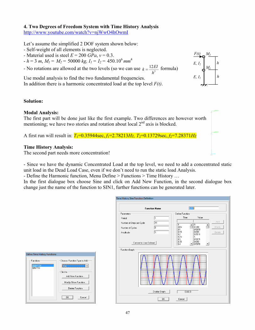
4. Two Degrees of Freedom System with Time History Analysis http://www.youtube.com/watch?v=njWwO4hOwmI Let’s assume the simplified 2 DOF system shown below: - Self-weight of all elements is neglected. - Material used is steel E = 200 GPa, v = 0.3. - h = 3 m, M1 = M2 = 50000 kg, I1 = I2 = 450.106 mm4 - No rotations are allowed at the two levels (so we can use

312

hEIk = formula)

Use modal analysis to find the two fundamental frequencies. In addition there is a harmonic concentrated load at the top level F(t). Solution: Modal Analysis: The first part will be done just like the first example. Two differences are however worth mentioning; we have two stories and rotation about local 2nd axis is blocked. A first run will result in: T1=0.35944sec, f1=2.78213Hz, T2=0.13729sec, f2=7.28371Hz Time History Analysis: The second part needs more concentration! - Since we have the dynamic Concentrated Load at the top level, we need to add a concentrated static unit load in the Dead Load Case, even if we don’t need to run the static load Analysis. - Define the Harmonic function, Menu Define > Functions > Time History … In the first dialogue box choose Sine and click on Add New Function, in the second dialogue box change just the name of the function to SIN1, further functions can be generated later.

E, I1

E, I2M1

M2F(t)

h

h

48

- Define a new Load case for the Time History Analysis, Menu Define > Load Cases … Click on Add New Load Case … button

Scale Factor has been used because the unit dead load introduced previously (1N) is not big enough to move the system. (1E7 is a bit exaggerated). If you want to see the transient solution (starting from time t = 0 sec) click on Transient. It is highly recommended to use Time Step Data in accordance with Time History Function Definition, in this case SIN1, to avoid direct integration numerical perturbation. To neglect the effect of damping, click on Modify/Show… button under other parameter and put 0 for constant damping for all modes. Now Run! The analysis A good way to display the results for time history analysis is to use the built-in plot engine Menu Display > Show Plot Functions…

First choose Time History

Choose a name for the

load case

For Steady state choose

Periodic

Change Function to SIN1 and Scale factor to 1e7 then

click on Add

Change to finer time

step

Neglect the damping effect

49

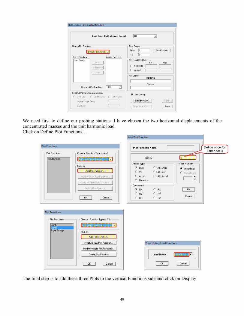
We need first to define our probing stations. I have chosen the two horizontal displacements of the concentrated masses and the unit harmonic load. Click on Define Plot Functions…

The final step is to add these three Plots to the vertical Functions side and click on Display

Define once for 2 then for 3

50

Period of SIN1 = 1sec (Periodic)

Period of SIN1 = 0.36sec (Transient)

51

Period of SIN1 = 0.14sec (Transient)

Period of SIN1 = 0.157sec (Periodic)

Note that in the last run, Joint3 is still the node where the load is applied. But in this case it is not moving at all. Can you explain why? 5. Additional Examples 5.1. Find the fundamental period and frequency of the following beams with a lumped mass at midspan. Compare the results with hand calculated formula. M = 10 000 kg, E = 200 GPa, I = 150 106 mm4, l = 6m

M

l/2l/2

E,I

M

l/2l/2

E,I

52

5.2. Repeat example 3 using the simplified model shown below, made of one vertical column, and three concentrated masses. 5.3. Try to use the weight as masses and compare the results.

I1

I2

I3

M1

M2

M3

53

E, Ih

P Δ

Lab 6 – Geometric Nonlinearity and P-Δ effect 1. P-Δ Effect http://www.youtube.com/watch?v=B6ZPNb-XIBQ This example will illustrate how to use SAP2000 to include geometric nonlinearity in a static analysis. In this case, the deformation due to an applied static vertical load will include second order effects caused by the eccentricity of the axial load. E= 200 GPa h = 3 m Δ = 10 cm P = 100 kN Default Section i. General Definitions Choose (kN, m, C) as principal units and a grid system X(0, 0.1), Y(0), Z(0, 3) ii. Material and Section Definition Define Material (MAT) having Self-Weight = 0, E = 200 GPa and v = 0.3 Don’t define frame section, just draw the model, and then change the default section material to MAT iii. Drawing the Model Draw a frame from point p1(0,0,0) to p2(0,0,3) and finish it in point p3(0.1,0,3) iv. Boundary Displacement Conditions Assign fixed restraints to the base. v. Loading Condition Assign a concentrated load under the DEAD load case to joint p3 equal to -100 kN in the Global Z axis. There are two main methods to include P-Delta effects in Sap2000, we will use only one in this example Menu Define > Load Cases …

54

vi. Analyse the System Select XZ plane frame in the analysis option to reduce the problem size, then Run the analysis. vii. Display Output Open a second display window to see the linear and non linear results on the same screen. (Small triangle at the top left of the main graphic interface window, see red circle below)

Difference in the Horizontal (U1) Displacement between Linear and non Nonlinear analysis

Select nonlinear type

Select P-Delta

Add the Dead

Choose a name for the load case

Choose Static load case

55

10.0

0

ltotal

Δ

Flexural Moment (M3-3), Constant in the column for the classical linear analysis and

varying according to the deformation shape for the nonlinear analysis. Note that those values are obtained using a scale of 10 times the actual vertical loading condition. 2. Geometric Nonlinearity http://www.youtube.com/watch?v=K9dDpBQbUsk The second example will illustrate how to include large deflections in a static nonlinear analysis for a typical case of geometric instability. Material E= 200 GPa, v = 0.3, ρ = 0 kN/m3 Section A = 4000 mm4

P = 10 kN ltotal = 4 m Run the analysis twice one with Δ1 = 10 cm and the other with Δ2 = 5 cm. For simplicity assume all the nodes to be articulated (truss structure). To solve this example follow the same steps as usual, the only difference is the definition of the static nonlinear analysis case, named here NL. You may need to specify the moment releases of the members.

56

Run the analysis twice, the first run with Δ1 = 10 cm.

For Δ1 = 10 cm, there is no inflection (members in compression)

For the second run with Δ2 = 5 cm, it is better to do a database editing instead of redrawing the whole structure from scratch again. Go to Menu Edit > Interactive Database Editing … Select Model Definition > Connectivity Data > Joints Coordinates > Table: Joint Coordinates Then change the Z coordinate of the appropriate node from 0.1 to 0.05

Static Nonlinear

P-Delta + Large displacements

57

E, Ih

PyPx

For Δ2 = 5 cm, the nonlinear analysis leads to an inflected beam (members in tension) whereas the

linear analysis still shows a compression in the members. As you can see from these two runs, we ended up with two completely different results for the linear and the nonlinear analysis. 3. Additional Example Repeat example 1 for the column loaded with vertical and lateral forces. Try different values of Py and see what happens when the vertical load gets close to the critical value Pcr (Euler critical load for the first mode).

58

Supplemental Material for SAP2000 Convention used

1. Axis and Convention: The default orientation of the Global system of coordinates X, Y, Z is +Z upward and Gravity acting in –Z. Right-hand rule and color convention

Right-hand convention for positive rotation

1

2

3

59

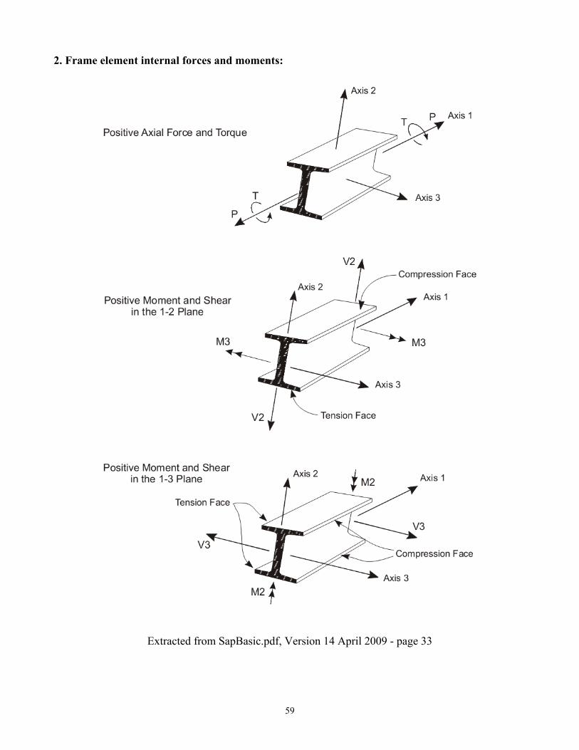
2. Frame element internal forces and moments:

Extracted from SapBasic.pdf, Version 14 April 2009 - page 33

60

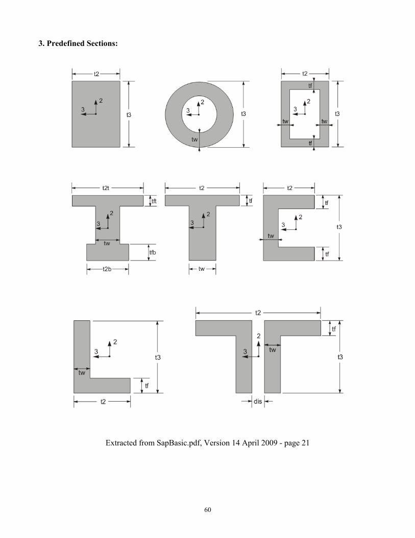
3. Predefined Sections:

Extracted from SapBasic.pdf, Version 14 April 2009 - page 21

61

4. Shell Element Convention:

Four and Three nodes shell element connectivity and face definition Extracted from SapBasic.pdf, Version 14 April 2009 - page 38

62

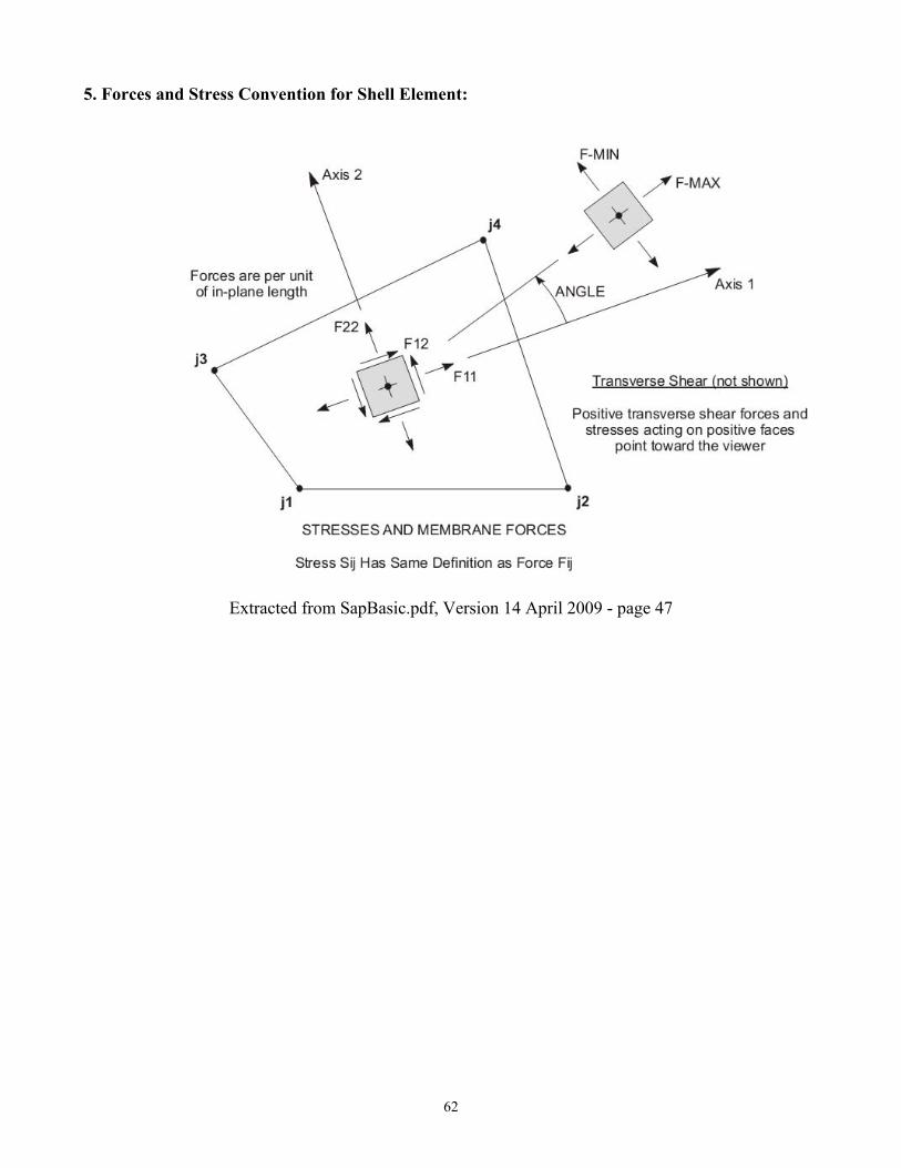
5. Forces and Stress Convention for Shell Element:

Extracted from SapBasic.pdf, Version 14 April 2009 - page 47