CDS 301 Spring, 2013 CH3: MATLAB 3-D Visualization February 07, 2013 - TBD Jie Zhang Copyright ©
81
CDS 301 Spring, 2013 CH3: MATLAB 3-D Visualization February 07, 2013 - TBD Jie Zhang Copyright ©
-
Upload
augustine-logan -
Category
Documents
-
view
221 -
download
0
Transcript of CDS 301 Spring, 2013 CH3: MATLAB 3-D Visualization February 07, 2013 - TBD Jie Zhang Copyright ©
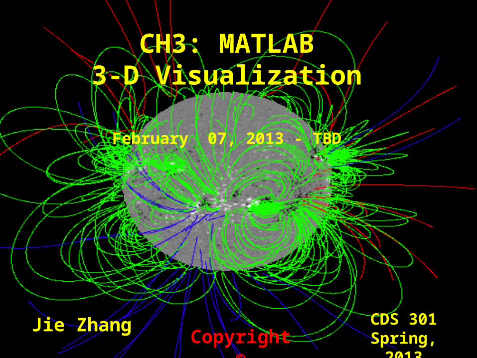
CDS 301Spring, 2013
CH3: MATLAB3-D Visualization
February 07, 2013 - TBD
Jie ZhangCopyright ©
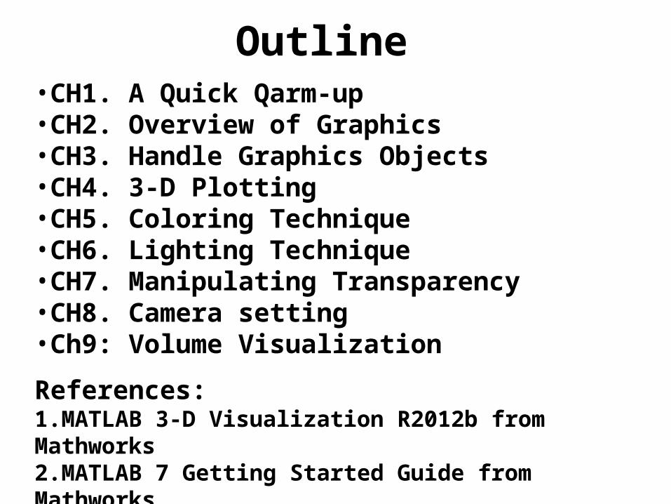
Outline•CH1. A Quick Qarm-up•CH2. Overview of Graphics•CH3. Handle Graphics Objects•CH4. 3-D Plotting•CH5. Coloring Technique•CH6. Lighting Technique•CH7. Manipulating Transparency•CH8. Camera setting•Ch9: Volume Visualization
References: 1.MATLAB 3-D Visualization R2012b from Mathworks2.MATLAB 7 Getting Started Guide from Mathworks
Chapter 1
A Quick Warm Up
(February 07, 2013)

Getting StartedFor more details of how to get started with MATLAB
1.“MATLAB 7 Getting Started Guide from Mathworks”
• PDF document, 280 page• Available at
http://spaceweather.gmu.edu/jzhang/teaching/2013_CDS301_Spring/resource.html
2. “Introduction to Matlab”• PPT presentation from CDS130• Available at
http://spaceweather.gmu.edu/jzhang/teaching/2013_CDS301_Spring/class_notes.html
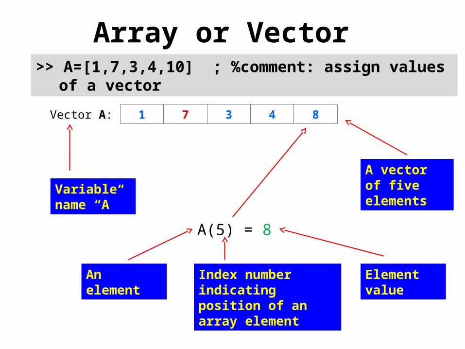
Vector A: 1 7 3 4 8
A(5) = 8
>> A=[1,7,3,4,10] ; %comment: assign values of a vector
Variable name “A”
A vector of five elements
Index number indicating position of an array element
An element Element value
Array or Vector
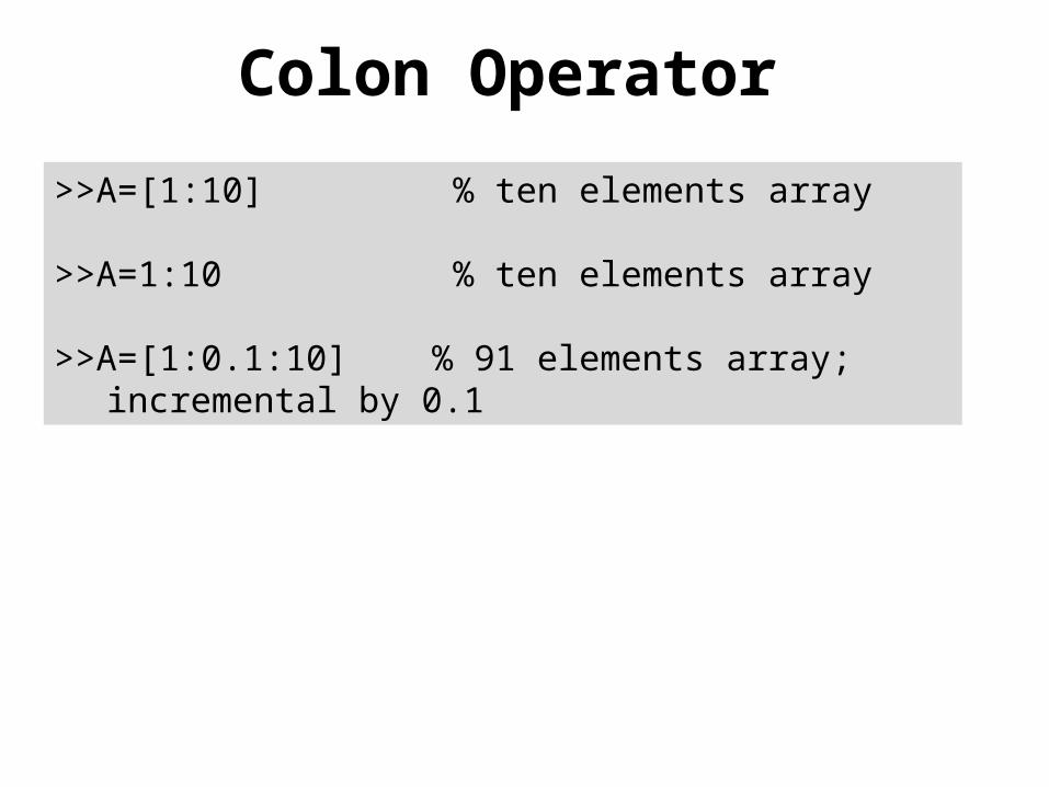
Colon Operator
>>A=[1:10] % ten elements array
>>A=1:10 % ten elements array >>A=[1:0.1:10] % 91 elements array; incremental by 0.1
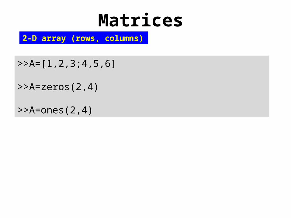
Matrices
>>A=[1,2,3;4,5,6]
>>A=zeros(2,4)
>>A=ones(2,4)
2-D array (rows, columns)
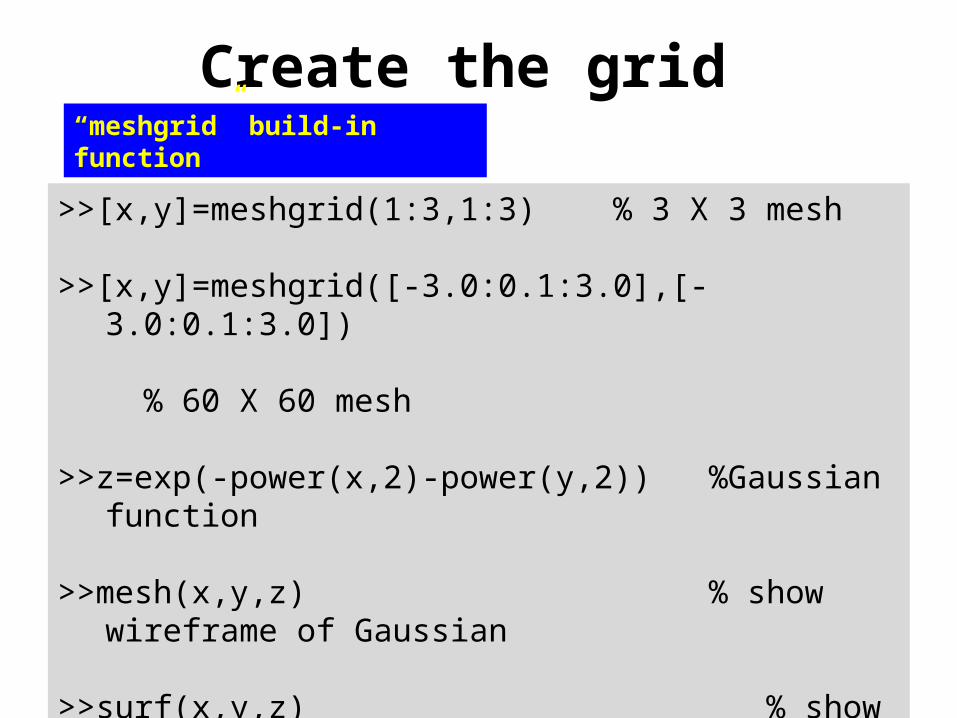
Create the grid
>>[x,y]=meshgrid(1:3,1:3) % 3 X 3 mesh
>>[x,y]=meshgrid([-3.0:0.1:3.0],[-3.0:0.1:3.0]) % 60 X 60 mesh
>>z=exp(-power(x,2)-power(y,2)) %Gaussian function
>>mesh(x,y,z) % show wireframe of Gaussian
>>surf(x,y,z) % show surface
“meshgrid” build-in function
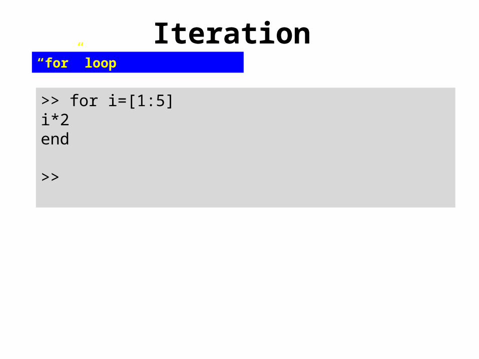
Iteration
>> for i=[1:5]i*2end
>>
“for” loop
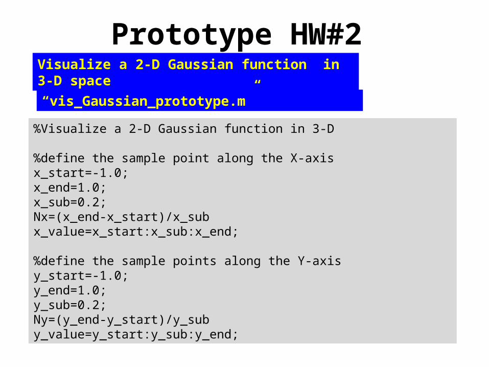
Prototype HW#2
%Visualize a 2-D Gaussian function in 3-D
%define the sample point along the X-axis x_start=-1.0; x_end=1.0; x_sub=0.2; Nx=(x_end-x_start)/x_subx_value=x_start:x_sub:x_end;
%define the sample points along the Y-axis y_start=-1.0; y_end=1.0; y_sub=0.2; Ny=(y_end-y_start)/y_sub y_value=y_start:y_sub:y_end;
Visualize a 2-D Gaussian function in 3-D space
“vis_Gaussian_prototype.m”
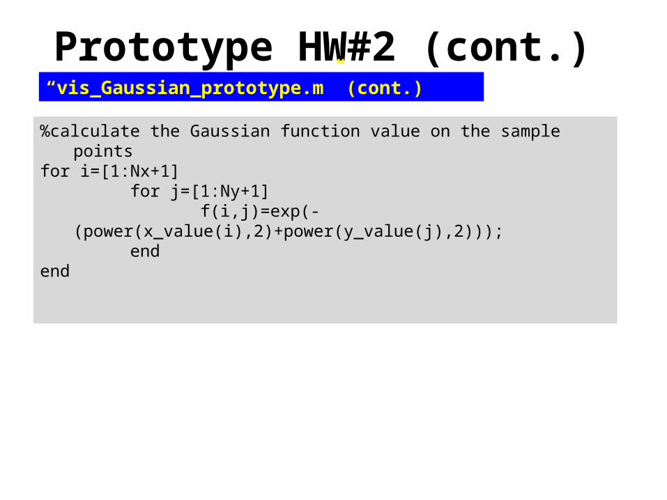
Prototype HW#2 (cont.)
%calculate the Gaussian function value on the sample points for i=[1:Nx+1] for j=[1:Ny+1] f(i,j)=exp(-(power(x_value(i),2)+power(y_value(j),2))); end end
“vis_Gaussian_prototype.m” (cont.)
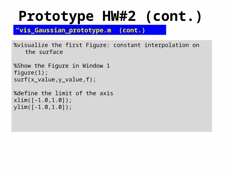
Prototype HW#2 (cont.)
%visualize the first Figure: constant interpolation on the surface
%Show the Figure in Window 1 figure(1); surf(x_value,y_value,f);
%define the limit of the axis xlim([-1.0,1.0]); ylim([-1.0,1.0]);
“vis_Gaussian_prototype.m” (cont.)
Prototype HW#2 (cont.)
%set up the green color
colormap([0,1,0])
“vis_Gaussian_prototype.m” (cont.)
%set up the green color colormap([0,1,0])
Prototype HW#2 (cont.)
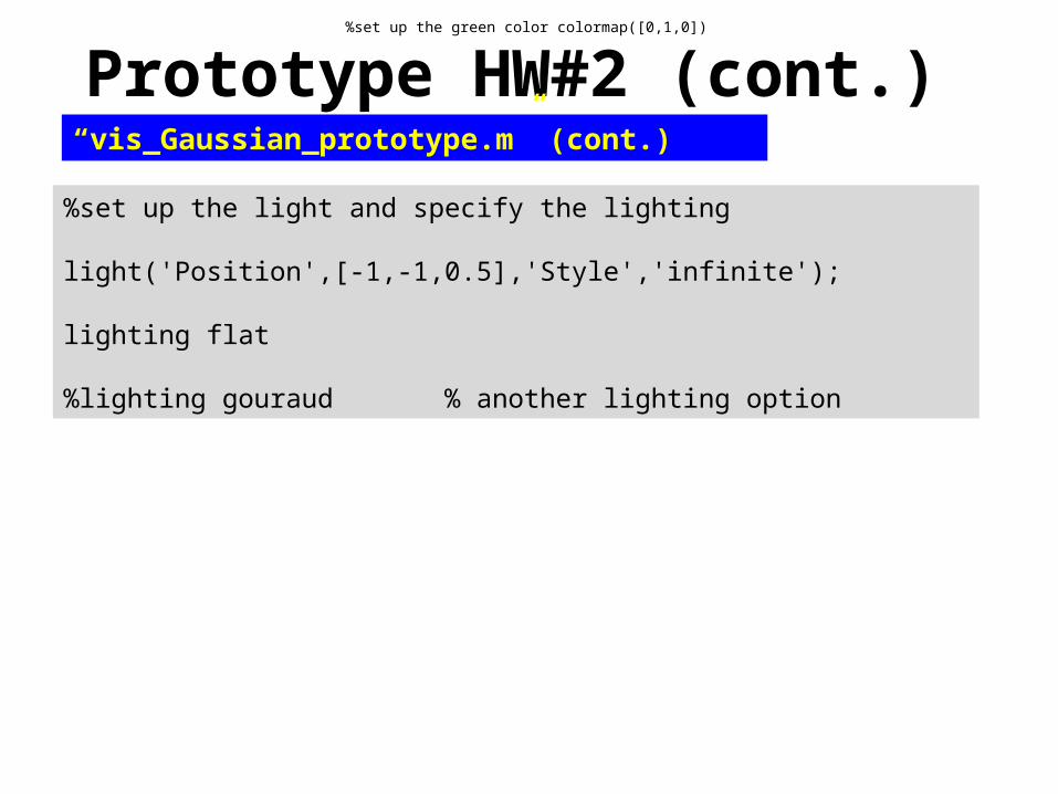
%set up the light and specify the lighting
light('Position',[-1,-1,0.5],'Style','infinite');
lighting flat
%lighting gouraud % another lighting option
“vis_Gaussian_prototype.m” (cont.)
%set up the green color colormap([0,1,0])
Prototype HW#2 (cont.)
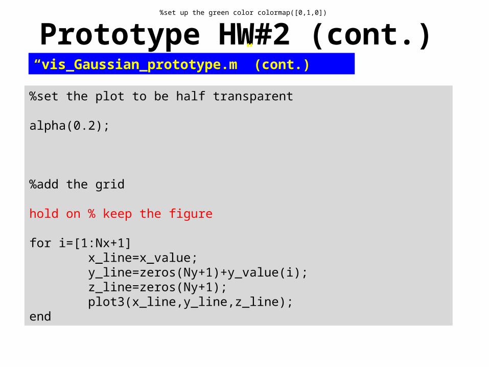
%set the plot to be half transparent
alpha(0.2);
“vis_Gaussian_prototype.m” (cont.)
%set up the green color colormap([0,1,0])
Prototype HW#2 (cont.)
%set the plot to be half transparent
alpha(0.2);
%add the grid
hold on % keep the figure
for i=[1:Nx+1] x_line=x_value; y_line=zeros(Ny+1)+y_value(i); z_line=zeros(Ny+1); plot3(x_line,y_line,z_line); end
“vis_Gaussian_prototype.m” (cont.)
%set up the green color colormap([0,1,0])
Prototype HW#2 (cont.)
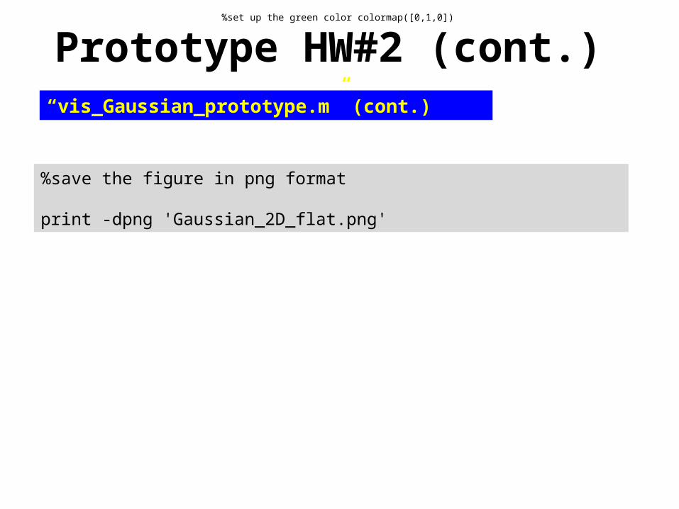
%save the figure in png format
print -dpng 'Gaussian_2D_flat.png'
“vis_Gaussian_prototype.m” (cont.)
%set up the green color colormap([0,1,0])

February 07, 2013 Stopped Here
Chapter 2
Overview of Graphics in Matlab
(February 12, 2013)
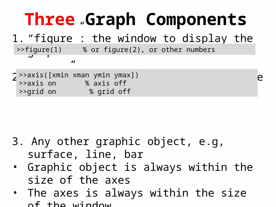
Three Graph Components1. “figure”: the window to display the graph
2. “axis”: the coordinate system of the graph
3. Any other graphic object, e.g, surface, line, bar• Graphic object is always within the size of the
axes• The axes is always within the size of the window• Each graphic component has a list of properties,
which can be modified through “Handles”
>>figure(1) % or figure(2), or other numbers
>>axis([xmin xman ymin ymax])>>axis on % axis off >>grid on % grid off
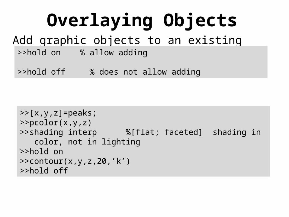
Overlaying ObjectsAdd graphic objects to an existing graph
>>hold on % allow adding
>>hold off % does not allow adding
>>[x,y,z]=peaks;>>pcolor(x,y,z)>>shading interp %[flat; faceted] shading in color, not in lighting>>hold on>>contour(x,y,z,20,’k’)>>hold off
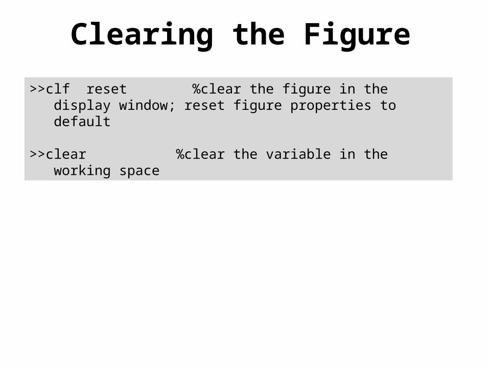
Clearing the Figure
>>clf reset %clear the figure in the display window; reset figure properties to default
>>clear %clear the variable in the working space
Chapter 3
Handle graphics objects
(February 12, 2013)
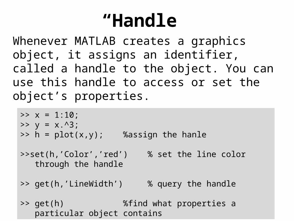
“Handle”Whenever MATLAB creates a graphics object, it assigns an identifier, called a handle to the object. You can use this handle to access or set the object’s properties.
>> x = 1:10;>> y = x.^3;>> h = plot(x,y); %assign the hanle >>set(h,’Color’,’red’) % set the line color through the handle
>> get(h,’LineWidth’) % query the handle
>> get(h) %find what properties a particular object contains
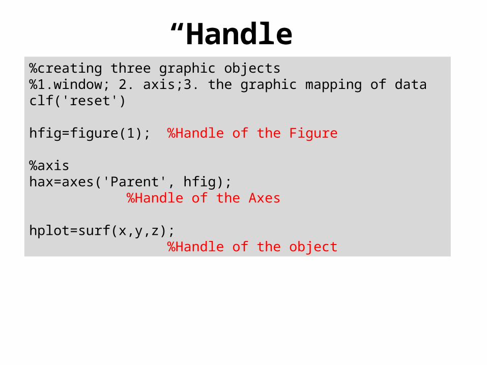
“Handle”%creating three graphic objects%1.window; 2. axis;3. the graphic mapping of dataclf('reset')
hfig=figure(1); %Handle of the Figure
%axishax=axes('Parent', hfig); %Handle of the Axes
hplot=surf(x,y,z); %Handle of the object
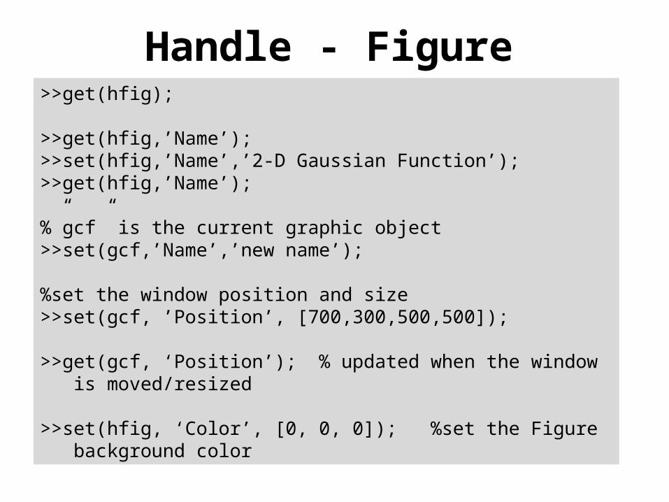
Handle - Figure>>get(hfig);
>>get(hfig,’Name’);>>set(hfig,’Name’,’2-D Gaussian Function’);>>get(hfig,’Name’);
%”gcf” is the current graphic object>>set(gcf,’Name’,’new name’);
%set the window position and size>>set(gcf, ’Position’, [700,300,500,500]);
>>get(gcf, ‘Position’); % updated when the window is moved/resized
>>set(hfig, ‘Color’, [0, 0, 0]); %set the Figure background color
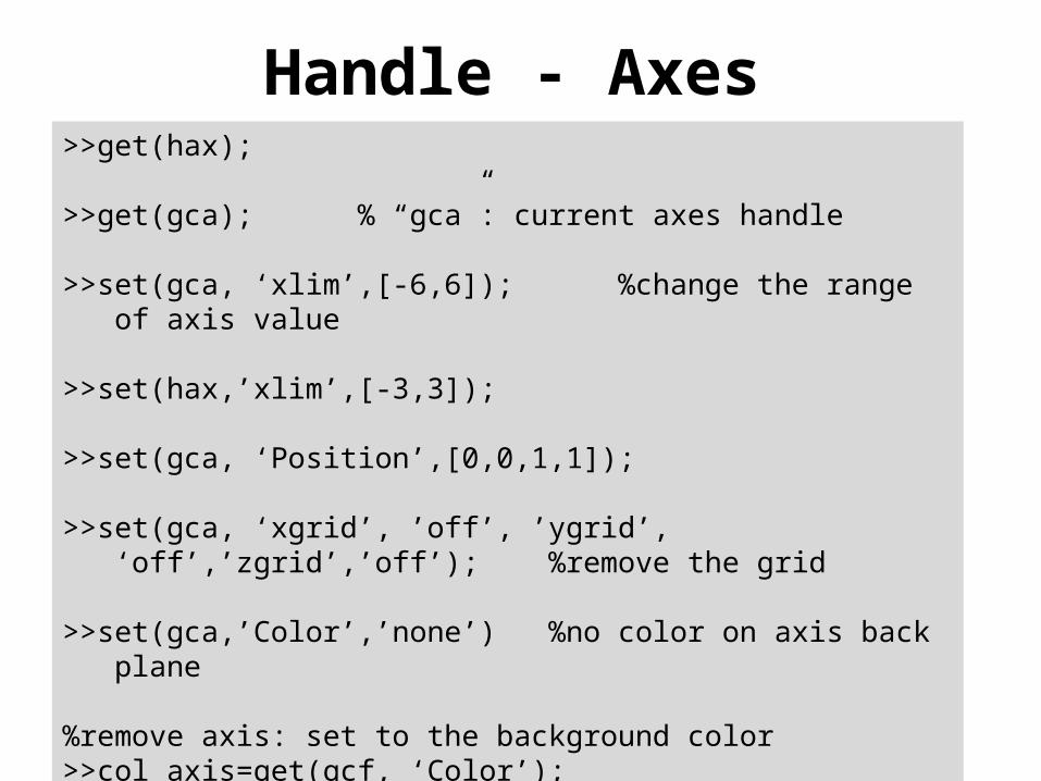
Handle - Axes>>get(hax);
>>get(gca); % “gca”: current axes handle
>>set(gca, ‘xlim’,[-6,6]); %change the range of axis value
>>set(hax,’xlim’,[-3,3]);
>>set(gca, ‘Position’,[0,0,1,1]);
>>set(gca, ‘xgrid’, ’off’, ’ygrid’, ‘off’,’zgrid’,’off’); %remove the grid
>>set(gca,’Color’,’none’) %no color on axis back plane
%remove axis: set to the background color>>col_axis=get(gcf, ‘Color’);>>set(gca, ‘xcolor’,col_axis);
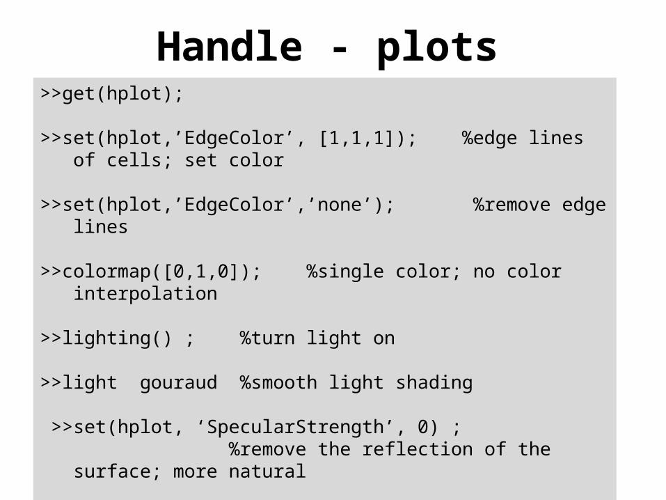
Handle - plots>>get(hplot);
>>set(hplot,’EdgeColor’, [1,1,1]); %edge lines of cells; set color
>>set(hplot,’EdgeColor’,’none’); %remove edge lines
>>colormap([0,1,0]); %single color; no color interpolation
>>lighting() ; %turn light on
>>light gouraud %smooth light shading
>>set(hplot, ‘SpecularStrength’, 0) ; %remove the reflection of the surface; more natural

February 12, 2013 Stopped Here
Chapter 4
3-D Plotting
(February 14, 2013)
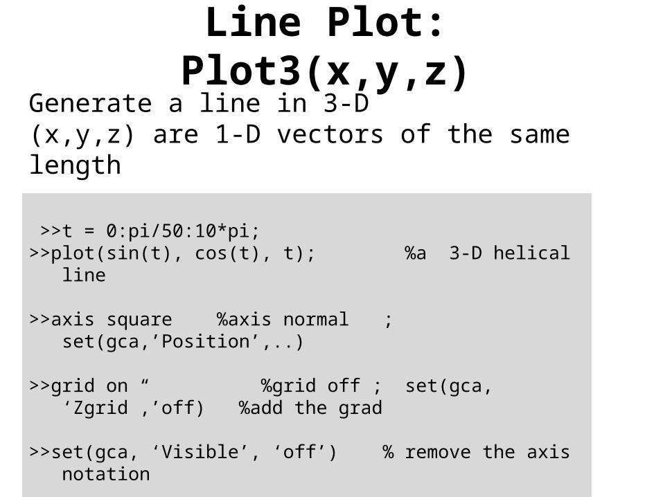
Line Plot: Plot3(x,y,z)
>>t = 0:pi/50:10*pi;>>plot(sin(t), cos(t), t); %a 3-D helical line
>>axis square %axis normal ; set(gca,’Position’,..)
>>grid on %grid off ; set(gca, ‘Zgrid”,’off) %add the grad
>>set(gca, ‘Visible’, ‘off’) % remove the axis notation
Generate a line in 3-D(x,y,z) are 1-D vectors of the same length
Line Plot: Plot3(x,y,z)
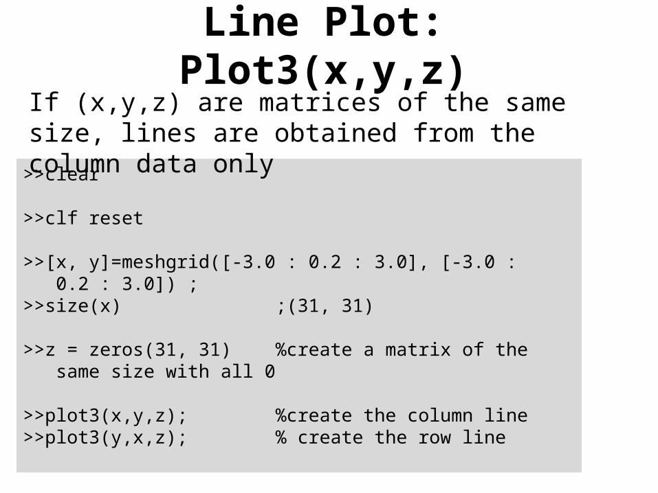
>>clear
>>clf reset
>>[x, y]=meshgrid([-3.0 : 0.2 : 3.0], [-3.0 : 0.2 : 3.0]) ;>>size(x) ;(31, 31)
>>z = zeros(31, 31) %create a matrix of the same size with all 0
>>plot3(x,y,z); %create the column line>>plot3(y,x,z); % create the row line
If (x,y,z) are matrices of the same size, lines are obtained from the column data only
Line Plot: Plot3(x,y,z)
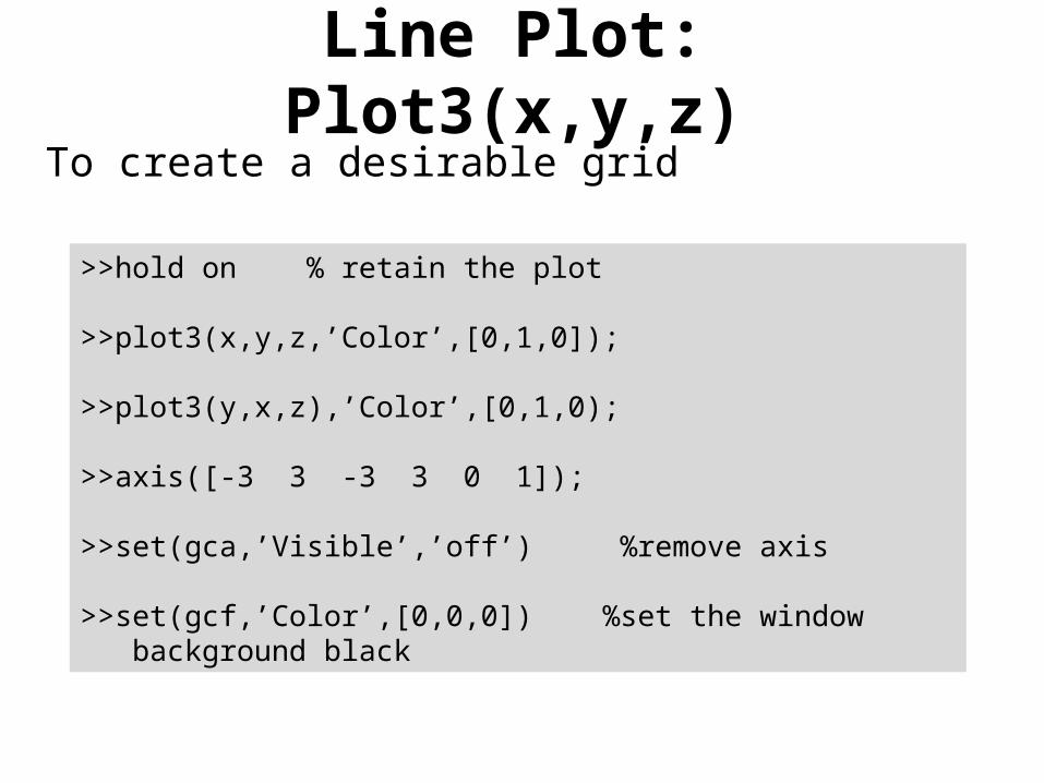
>>hold on % retain the plot
>>plot3(x,y,z,’Color’,[0,1,0]);
>>plot3(y,x,z),’Color’,[0,1,0);
>>axis([-3 3 -3 3 0 1]);
>>set(gca,’Visible’,’off’) %remove axis
>>set(gcf,’Color’,[0,0,0]) %set the window background black
To create a desirable grid
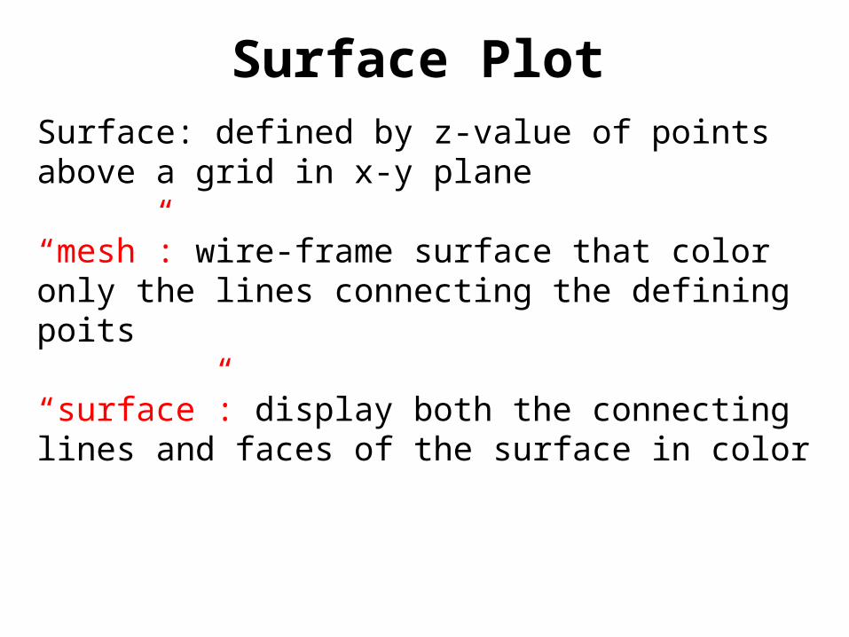
Surface PlotSurface: defined by z-value of points above a grid in x-y plane
“mesh”: wire-frame surface that color only the lines connecting the defining poits
“surface”: display both the connecting lines and faces of the surface in color
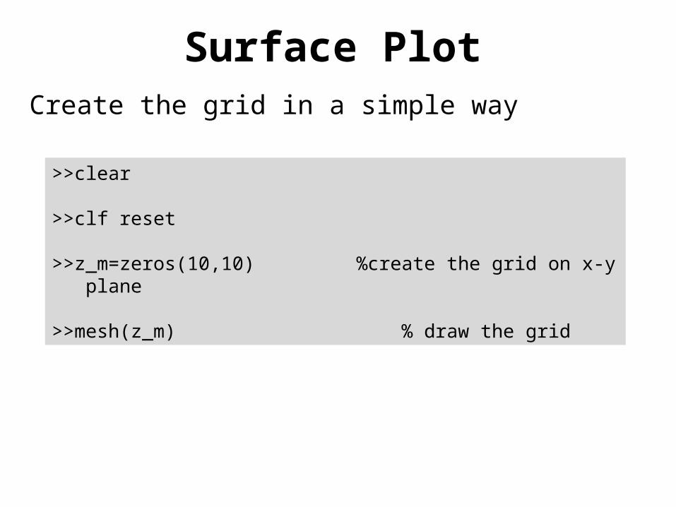
Surface PlotCreate the grid in a simple way
>>clear
>>clf reset
>>z_m=zeros(10,10) %create the grid on x-y plane
>>mesh(z_m) % draw the grid
Chapter 5
Coloring Technique
(February 14, 2013)
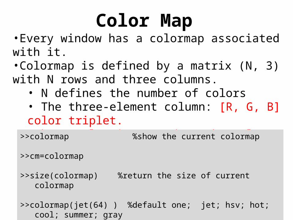
Color Map•Every window has a colormap associated with it.•Colormap is defined by a matrix (N, 3) with N rows and three columns.
• N defines the number of colors• The three-element column: [R, G, B] color triplet.•The Z value is mapped to the color range [1,N]
>>colormap %show the current colormap
>>cm=colormap
>>size(colormap) %return the size of current colormap
>>colormap(jet(64) ) %default one; jet; hsv; hot; cool; summer; gray % 64 or N defines the number of colors
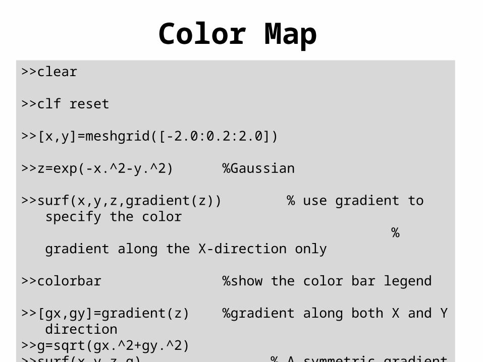
Color Map>>clear
>>clf reset
>>[x,y]=meshgrid([-2.0:0.2:2.0])
>>z=exp(-x.^2-y.^2) %Gaussian
>>surf(x,y,z,gradient(z)) % use gradient to specify the color % gradient along the X-direction only
>>colorbar %show the color bar legend
>>[gx,gy]=gradient(z) %gradient along both X and Y direction>>g=sqrt(gx.^2+gy.^2)>>surf(x,y,z,g) % A symmetric gradient map

Chapter 6
Lighting Technique
(February 14, 2013)
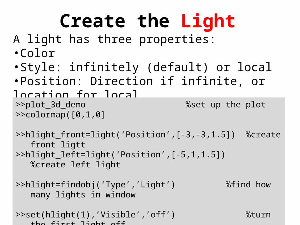
Create the LightA light has three properties:•Color•Style: infinitely (default) or local•Position: Direction if infinite, or location for local
>>plot_3d_demo %set up the plot>>colormap([0,1,0]
>>hlight_front=light(‘Position’,[-3,-3,1.5]) %create front ligtt>>hlight_left=light(‘Position’,[-5,1,1.5]) %create left light
>>hlight=findobj(‘Type’,’Light’) %find how many lights in window
>>set(hlight(1),’Visible’,’off’) %turn the first light off
>>set(hlight(1)’,’Visible’,’on’) %turn the first light on
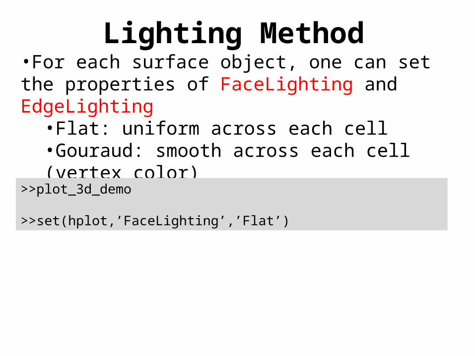
Lighting Method•For each surface object, one can set the properties of FaceLighting and EdgeLighting
•Flat: uniform across each cell•Gouraud: smooth across each cell (vertex color)•Phong: smooth across each cell (vertex normal)
>>plot_3d_demo
>>set(hplot,’FaceLighting’,’Flat’)
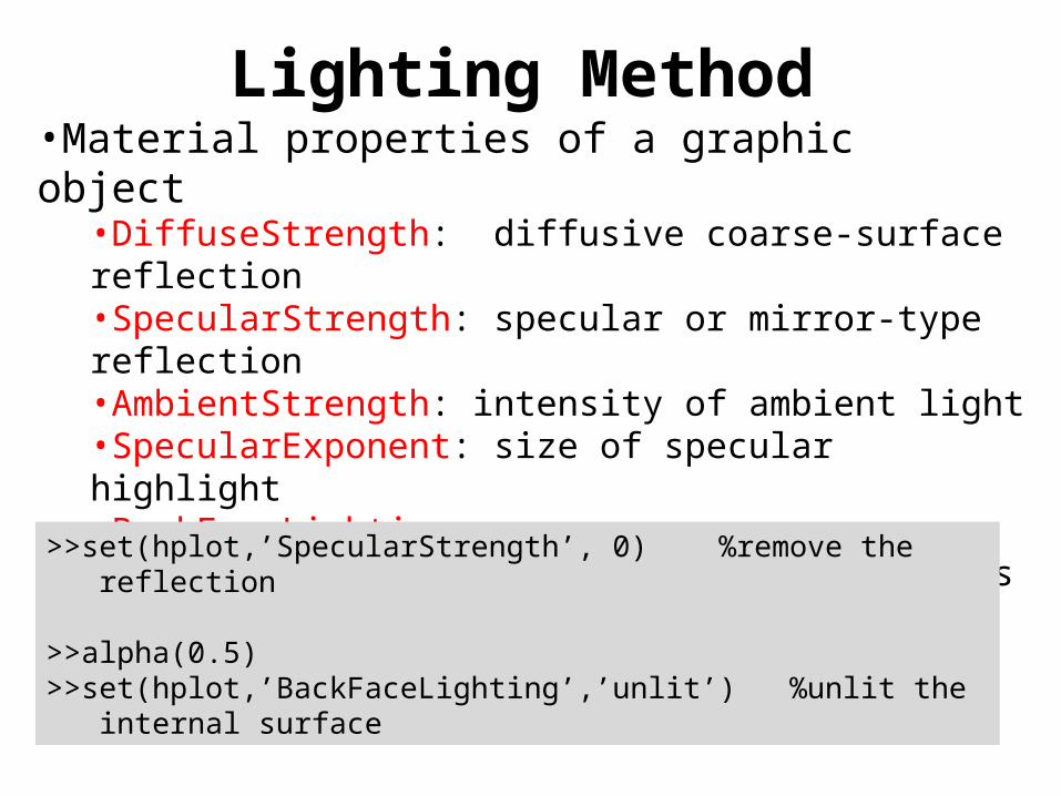
Lighting Method•Material properties of a graphic object
•DiffuseStrength: diffusive coarse-surface reflection•SpecularStrength: specular or mirror-type reflection•AmbientStrength: intensity of ambient light•SpecularExponent: size of specular highlight•BackFaceLighting
•‘reverselit’: internal surface reflects the light (default)•‘unlit’: internal surface does not reflect the light
>>set(hplot,’SpecularStrength’, 0) %remove the reflection
>>alpha(0.5)>>set(hplot,’BackFaceLighting’,’unlit’) %unlit the internal surface
Chapter 7
Manipulating Transparency
(February 21, 2013)
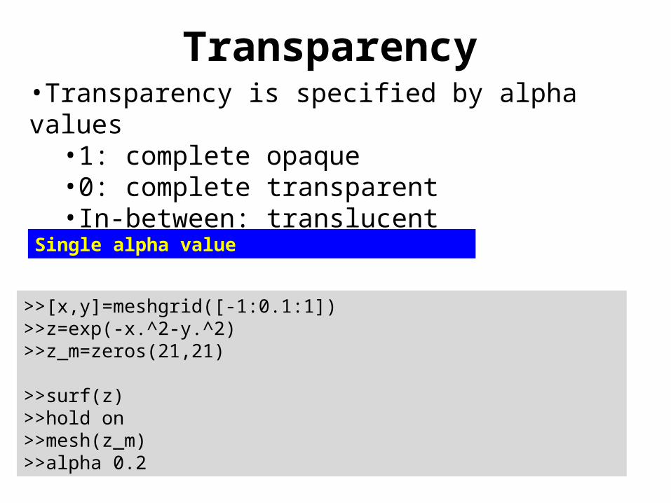
Transparency•Transparency is specified by alpha values
•1: complete opaque•0: complete transparent•In-between: translucent
>>[x,y]=meshgrid([-1:0.1:1])>>z=exp(-x.^2-y.^2)>>z_m=zeros(21,21)
>>surf(z)>>hold on>>mesh(z_m)>>alpha 0.2
Single alpha value
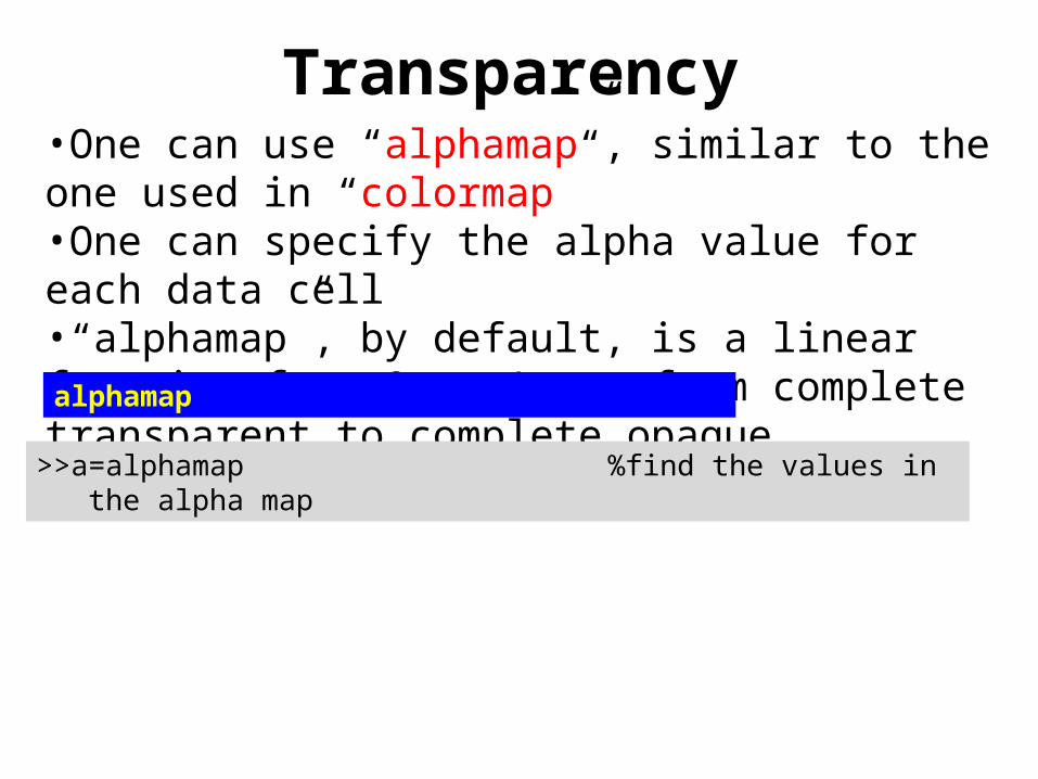
Transparency•One can use “alphamap”, similar to the one used in “colormap”•One can specify the alpha value for each data cell•“alphamap”, by default, is a linear function from 0 to 1, or from complete transparent to complete opaque
>>a=alphamap %find the values in the alpha map
alphamap
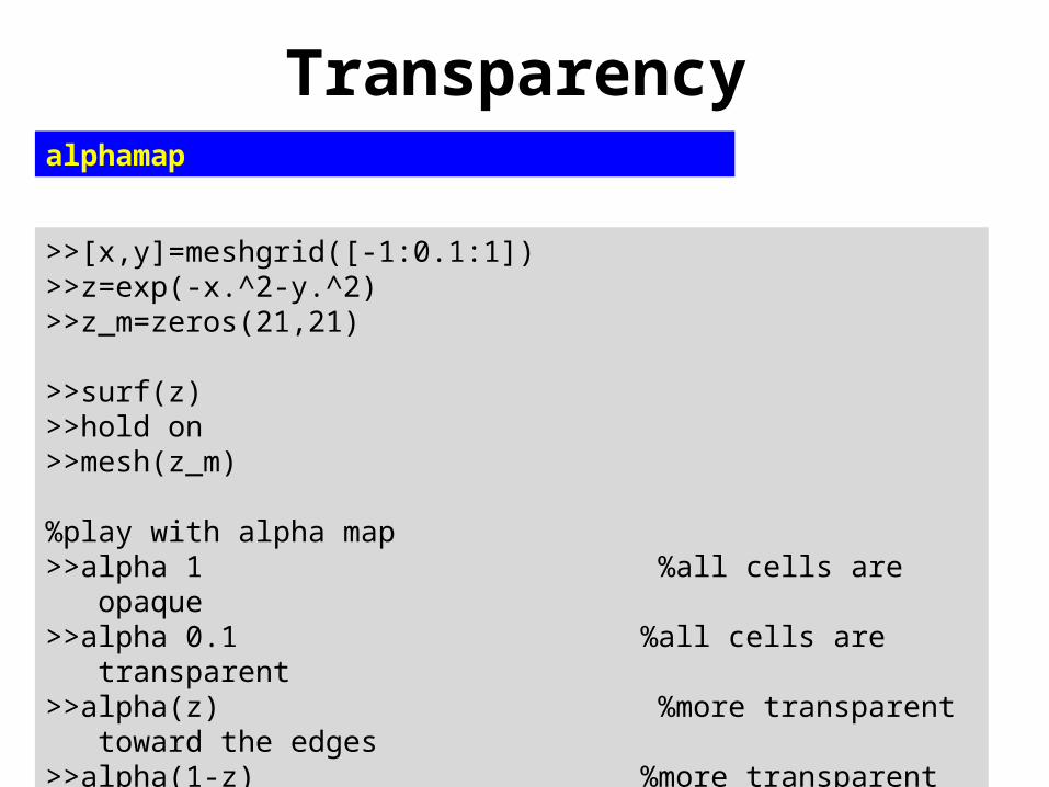
Transparencyalphamap
>>[x,y]=meshgrid([-1:0.1:1])>>z=exp(-x.^2-y.^2)>>z_m=zeros(21,21)
>>surf(z)>>hold on>>mesh(z_m)
%play with alpha map>>alpha 1 %all cells are opaque>>alpha 0.1 %all cells are transparent>>alpha(z) %more transparent toward the edges>>alpha(1-z) %more transparent toward the peak
Transparencyalphamap
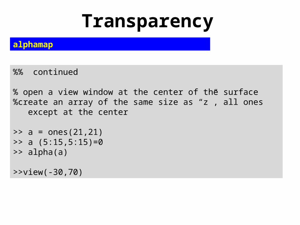
%% continued
% open a view window at the center of the surface%create an array of the same size as “z”, all ones except at the center
>> a = ones(21,21)>> a (5:15,5:15)=0>> alpha(a)
>>view(-30,70)
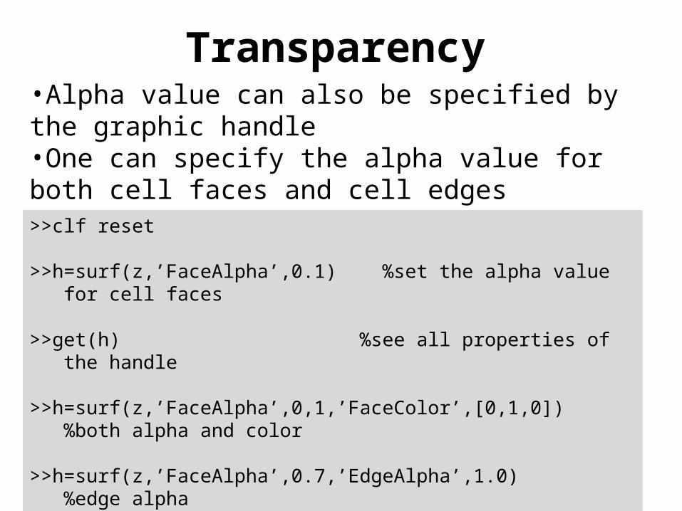
Transparency•Alpha value can also be specified by the graphic handle•One can specify the alpha value for both cell faces and cell edges>>clf reset
>>h=surf(z,’FaceAlpha’,0.1) %set the alpha value for cell faces
>>get(h) %see all properties of the handle
>>h=surf(z,’FaceAlpha’,0,1,’FaceColor’,[0,1,0]) %both alpha and color
>>h=surf(z,’FaceAlpha’,0.7,’EdgeAlpha’,1.0) %edge alpha
>>h=surf(z,'FaceAlpha',0.5,'EdgeAlpha',1.0,'FaceColor',[0,1,0],'EdgeColor',[1,0,0]) %what does this mean?
Chapter 8
Camera Setting
Camera Setting
•The appearance of a 3-D scene also depends on the viewing direction, changing the perspective and aspect ratio, zooming in or out, flying by, and so on.
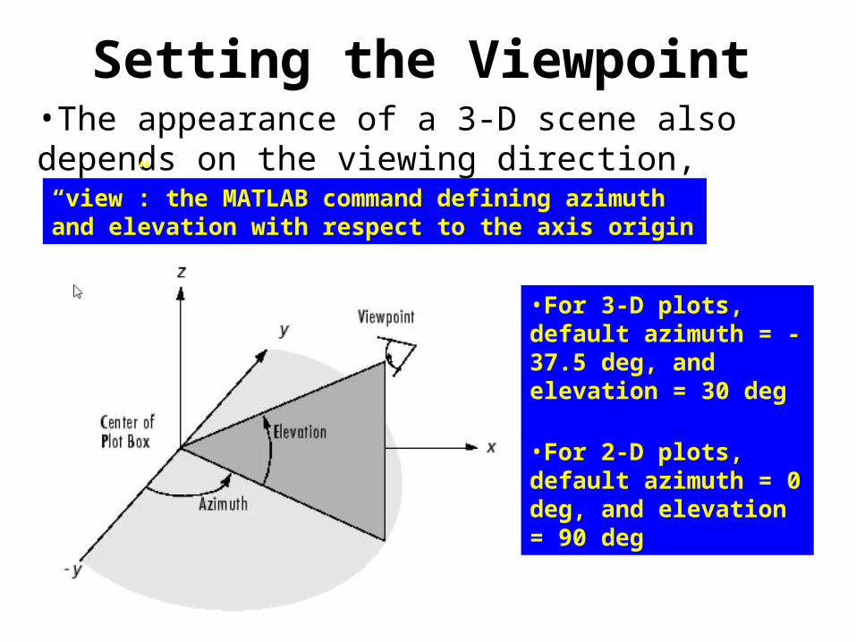
Setting the Viewpoint•The appearance of a 3-D scene also depends on the viewing direction,
“view”: the MATLAB command defining azimuth and elevation with respect to the axis origin
•For 3-D plots, default azimuth = -37.5 deg, and elevation = 30 deg
•For 2-D plots, default azimuth = 0 deg, and elevation = 90 deg
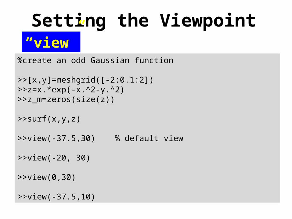
Setting the Viewpoint
%create an odd Gaussian function
>>[x,y]=meshgrid([-2:0.1:2])>>z=x.*exp(-x.^2-y.^2)>>z_m=zeros(size(z))
>>surf(x,y,z)
>>view(-37.5,30) % default view
>>view(-20, 30)
>>view(0,30)
>>view(-37.5,10)
“view”
Camera
Camera Toolbar: from the figure window’s View menu
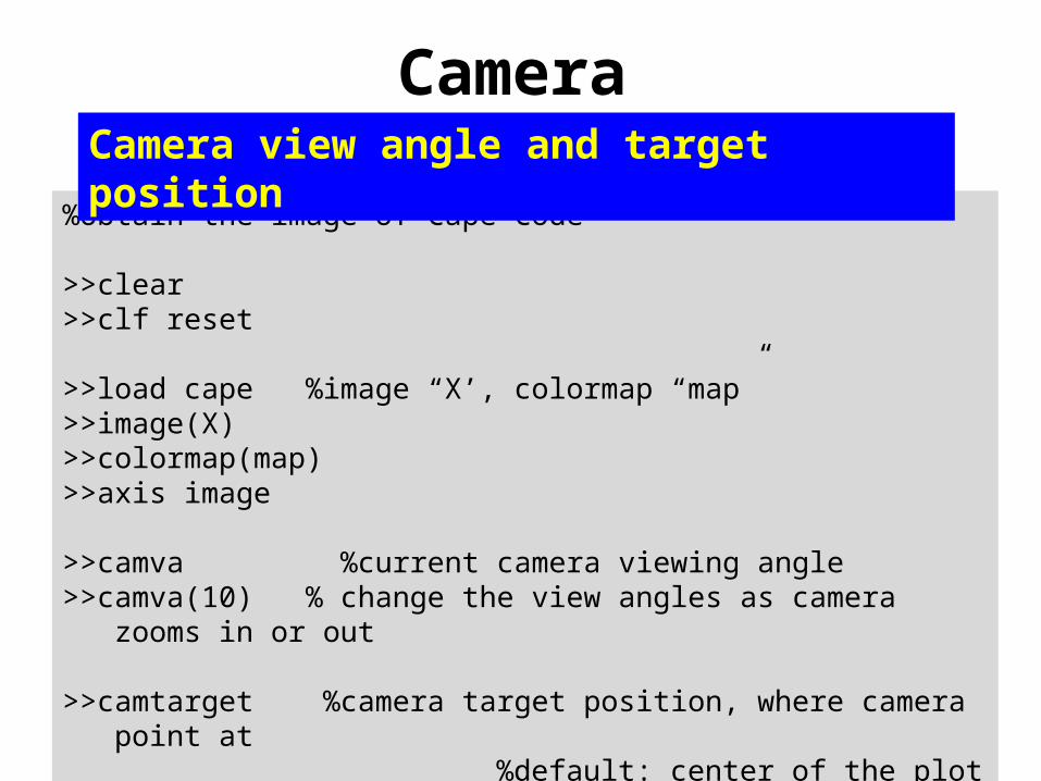
Camera
%obtain the image of Cape Code
>>clear>>clf reset
>>load cape %image “X’, colormap “map”>>image(X)>>colormap(map) >>axis image
>>camva %current camera viewing angle>>camva(10) % change the view angles as camera zooms in or out
>>camtarget %camera target position, where camera point at %default: center of the plot>>camtarget([10,10,0.5])
Camera view angle and target position
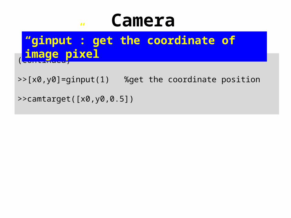
Camera
(continued)
>>[x0,y0]=ginput(1) %get the coordinate position
>>camtarget([x0,y0,0.5])
“ginput”: get the coordinate of image pixel
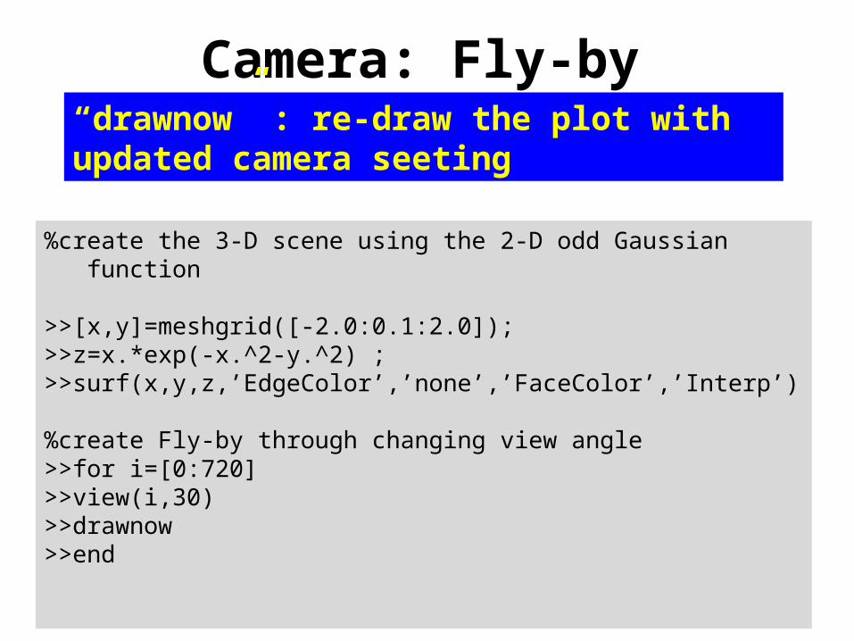
Camera: Fly-by
%create the 3-D scene using the 2-D odd Gaussian function
>>[x,y]=meshgrid([-2.0:0.1:2.0]);>>z=x.*exp(-x.^2-y.^2) ;>>surf(x,y,z,’EdgeColor’,’none’,’FaceColor’,’Interp’)
%create Fly-by through changing view angle>>for i=[0:720]>>view(i,30)>>drawnow>>end
“drawnow” : re-draw the plot with updated camera seeting
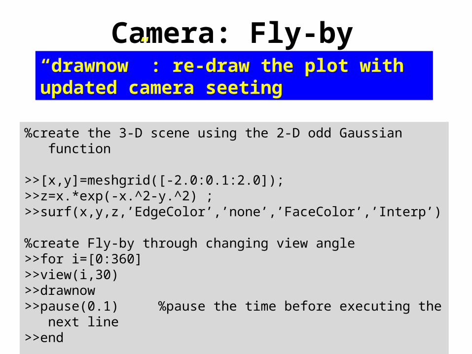
Camera: Fly-by
%create the 3-D scene using the 2-D odd Gaussian function
>>[x,y]=meshgrid([-2.0:0.1:2.0]);>>z=x.*exp(-x.^2-y.^2) ;>>surf(x,y,z,’EdgeColor’,’none’,’FaceColor’,’Interp’)
%create Fly-by through changing view angle>>for i=[0:360]>>view(i,30)>>drawnow>>pause(0.1) %pause the time before executing the next line>>end
“drawnow” : re-draw the plot with updated camera seeting
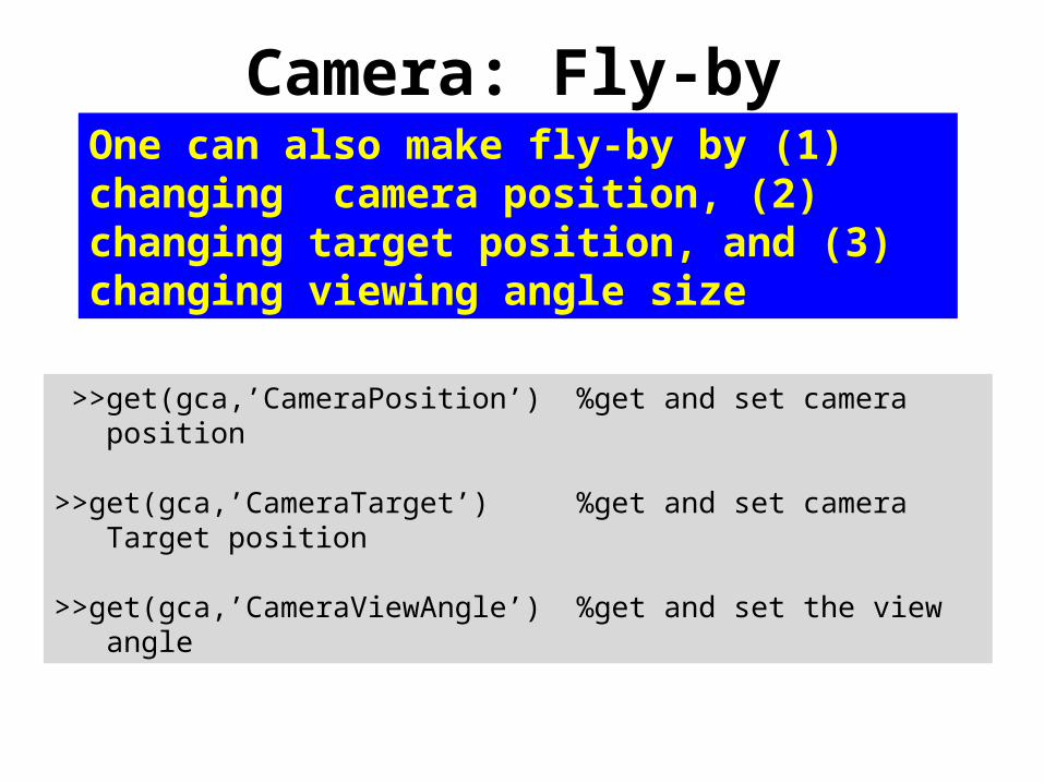
Camera: Fly-by
>>get(gca,’CameraPosition’) %get and set camera position
>>get(gca,’CameraTarget’) %get and set camera Target position
>>get(gca,’CameraViewAngle’) %get and set the view angle
One can also make fly-by by (1) changing camera position, (2) changing target position, and (3) changing viewing angle size
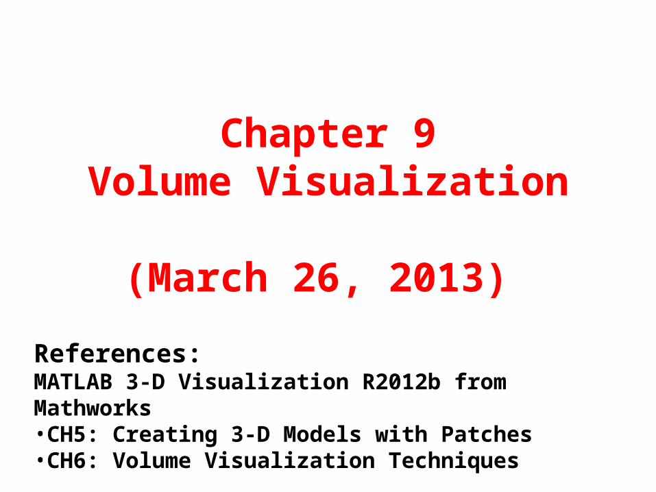
Chapter 9Volume Visualization
(March 26, 2013)
References: MATLAB 3-D Visualization R2012b from Mathworks•CH5: Creating 3-D Models with Patches•CH6: Volume Visualization Techniques
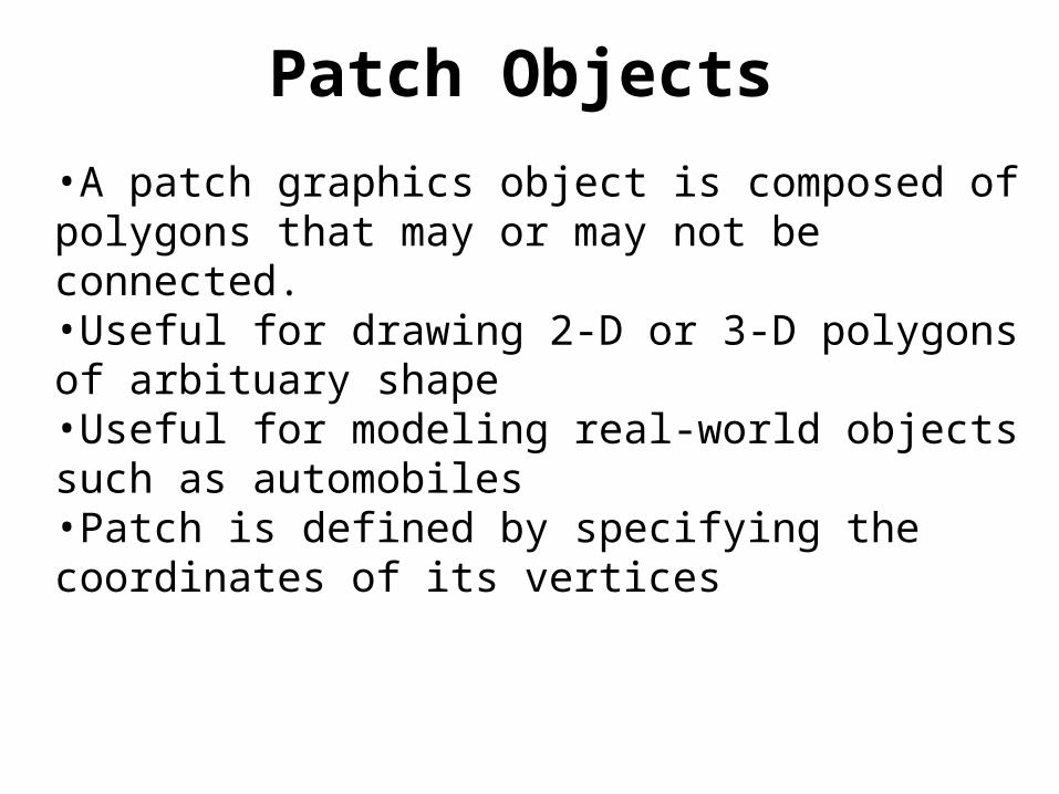
Patch Objects
•A patch graphics object is composed of polygons that may or may not be connected. •Useful for drawing 2-D or 3-D polygons of arbituary shape•Useful for modeling real-world objects such as automobiles•Patch is defined by specifying the coordinates of its vertices
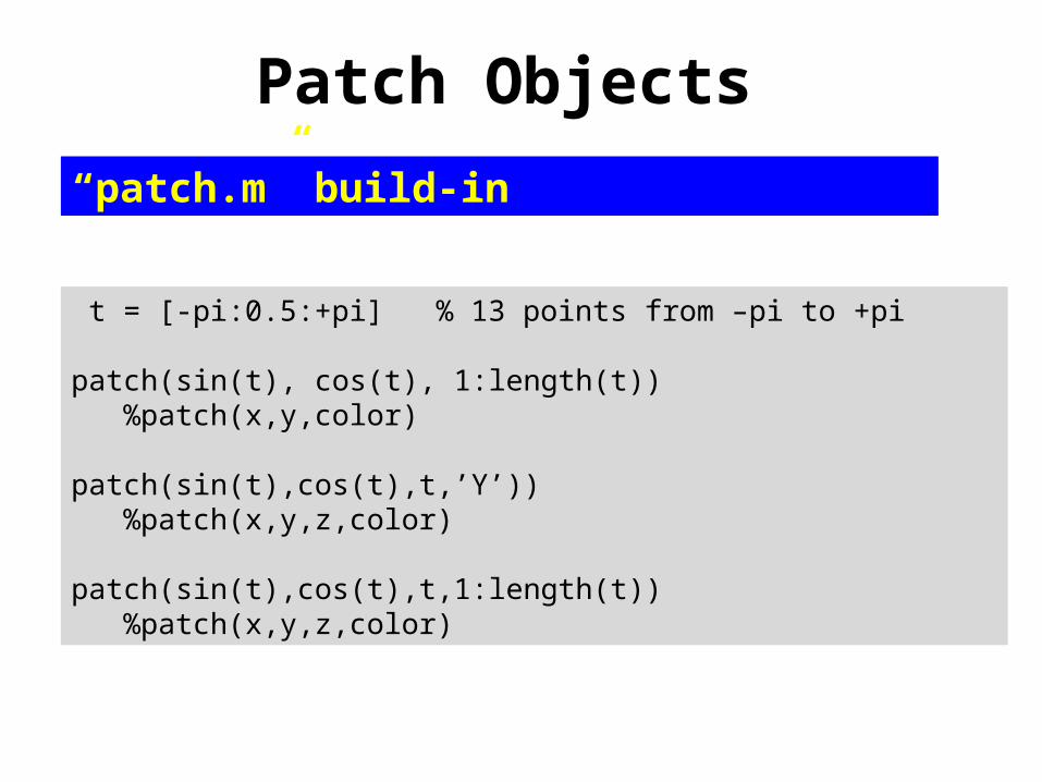
Patch Objects
t = [-pi:0.5:+pi] % 13 points from –pi to +pi
patch(sin(t), cos(t), 1:length(t)) %patch(x,y,color)
patch(sin(t),cos(t),t,’Y’)) %patch(x,y,z,color)
patch(sin(t),cos(t),t,1:length(t)) %patch(x,y,z,color)
“patch.m” build-in
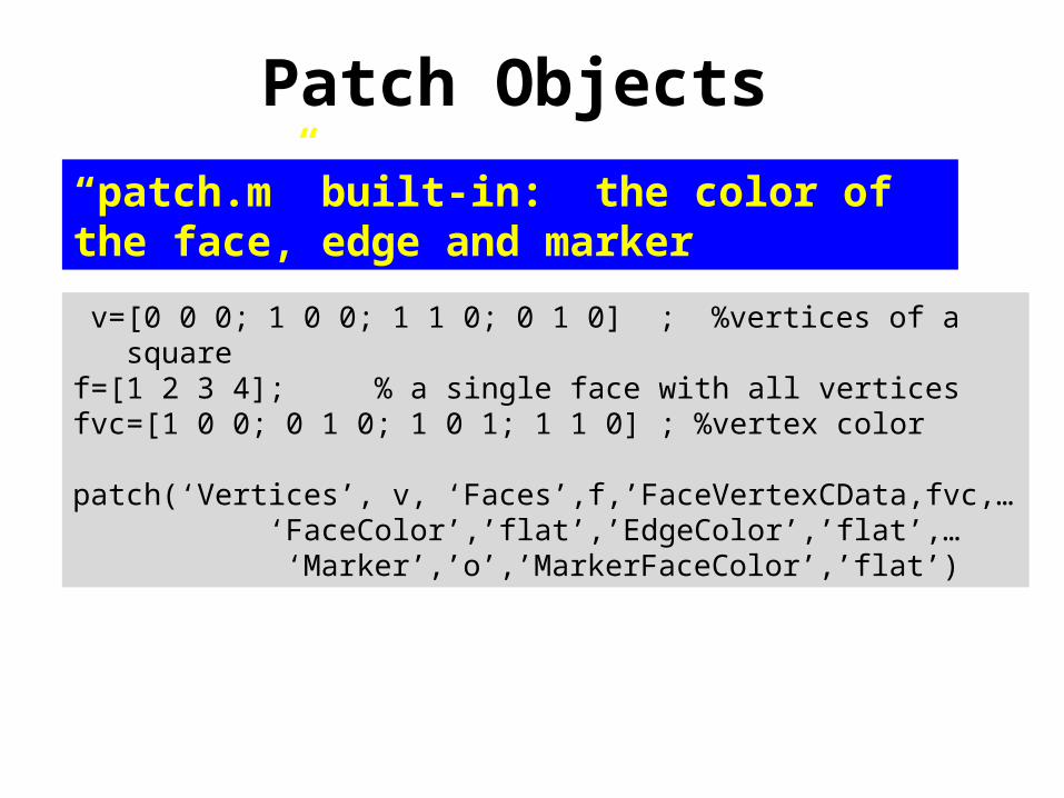
Patch Objects
v=[0 0 0; 1 0 0; 1 1 0; 0 1 0] ; %vertices of a squaref=[1 2 3 4]; % a single face with all verticesfvc=[1 0 0; 0 1 0; 1 0 1; 1 1 0] ; %vertex color
patch(‘Vertices’, v, ‘Faces’,f,’FaceVertexCData,fvc,… ‘FaceColor’,’flat’,’EdgeColor’,’flat’,… ‘Marker’,’o’,’MarkerFaceColor’,’flat’)
“patch.m” built-in: the color of the face, edge and marker
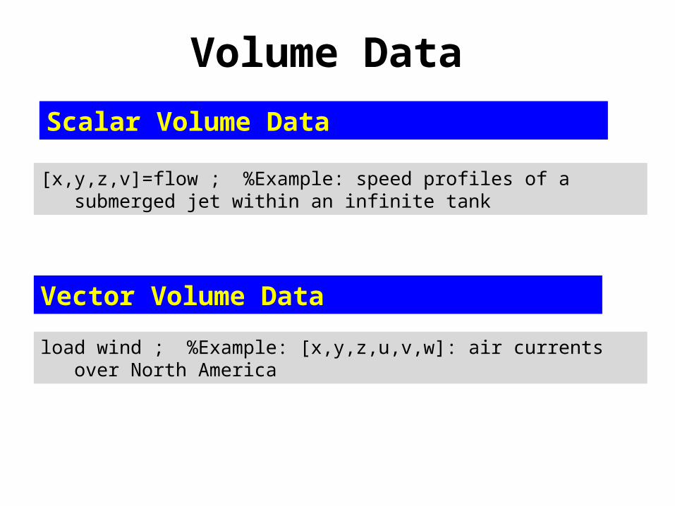
Volume Data
[x,y,z,v]=flow ; %Example: speed profiles of a submerged jet within an infinite tank
Scalar Volume Data
Vector Volume Data
load wind ; %Example: [x,y,z,u,v,w]: air currents over North America
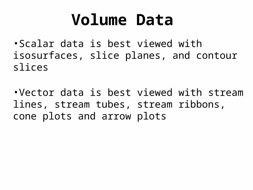
Volume Data•Scalar data is best viewed with isosurfaces, slice planes, and contour slices
•Vector data is best viewed with stream lines, stream tubes, stream ribbons, cone plots and arrow plots
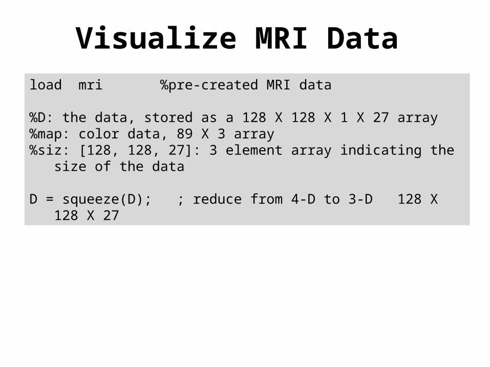
Visualize MRI Dataload mri %pre-created MRI data
%D: the data, stored as a 128 X 128 X 1 X 27 array%map: color data, 89 X 3 array%siz: [128, 128, 27]: 3 element array indicating the size of the data
D = squeeze(D); ; reduce from 4-D to 3-D 128 X 128 X 27
Visualize MRI Data
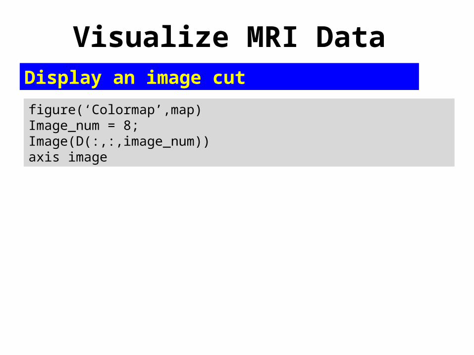
figure(‘Colormap’,map)Image_num = 8;Image(D(:,:,image_num))axis image
Display an image cut

Visualize MRI Data
contourslice(D,[ ],[ ], 10, 5) %
“contourslice.m” built-in
contourslice(D,[ ],[ ], [1, 12, 19, 27], 8) %display 4 slices view(3) %3-D viewaxis tight
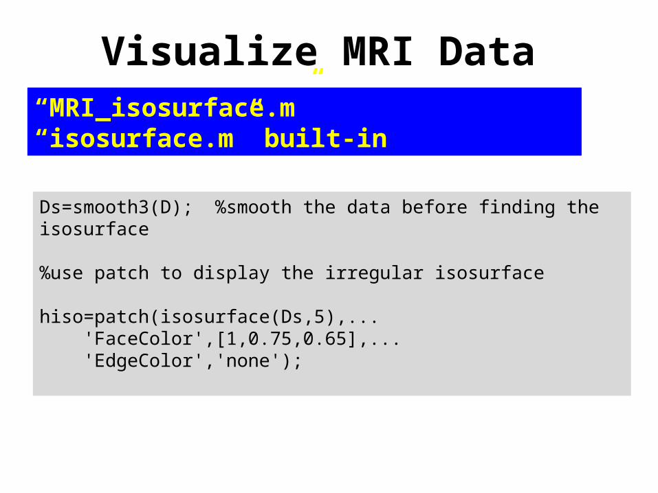
Visualize MRI Data“MRI_isosurface.m”“isosurface.m” built-in
Ds=smooth3(D); %smooth the data before finding the isosurface
%use patch to display the irregular isosurface
hiso=patch(isosurface(Ds,5),... 'FaceColor',[1,0.75,0.65],... 'EdgeColor','none');
Visualize MRI Data
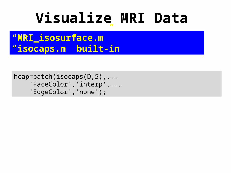
hcap=patch(isocaps(D,5),... 'FaceColor','interp',... 'EdgeColor','none');
“MRI_isosurface.m”“isocaps.m” built-in

(March 28, 2013)
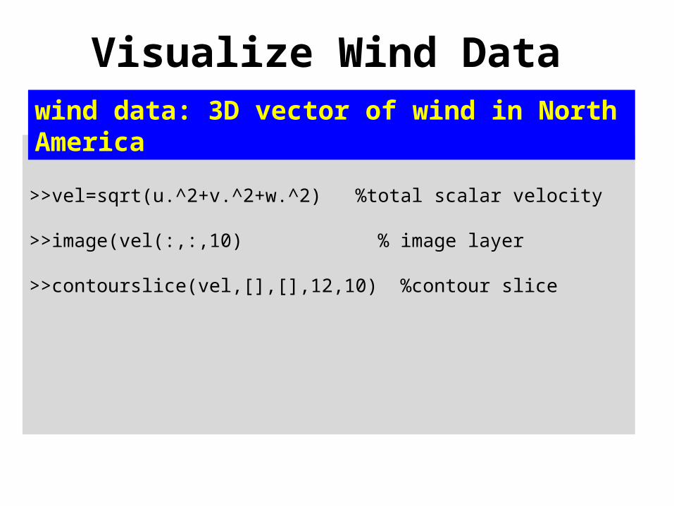
Visualize Wind Data
>>load wind
>>vel=sqrt(u.^2+v.^2+w.^2) %total scalar velocity
>>image(vel(:,:,10) % image layer
>>contourslice(vel,[],[],12,10) %contour slice
wind data: 3D vector of wind in North America
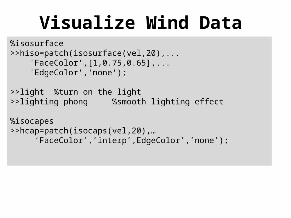
Visualize Wind Data%isosurface>>hiso=patch(isosurface(vel,20),... 'FaceColor',[1,0.75,0.65],... 'EdgeColor','none');
>>light %turn on the light>>lighting phong %smooth lighting effect
%isocapes>>hcap=patch(isocaps(vel,20),… ‘FaceColor’,’interp’,EdgeColor’,’none’);
Visualize Wind Data
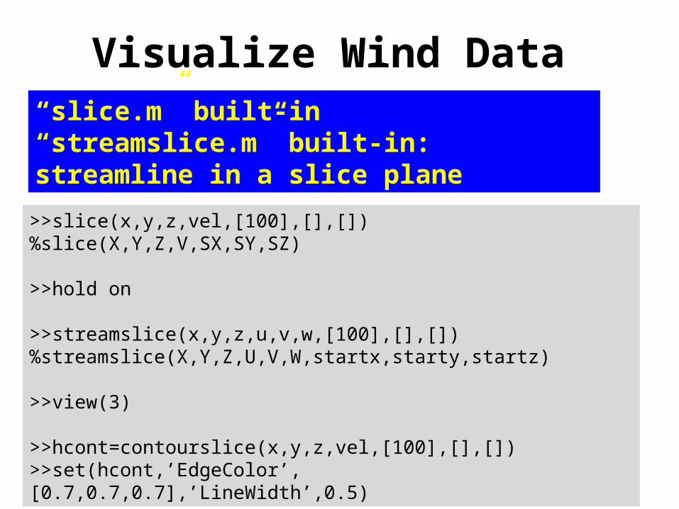
>>slice(x,y,z,vel,[100],[],[])%slice(X,Y,Z,V,SX,SY,SZ)
>>hold on
>>streamslice(x,y,z,u,v,w,[100],[],[]) %streamslice(X,Y,Z,U,V,W,startx,starty,startz)
>>view(3)
>>hcont=contourslice(x,y,z,vel,[100],[],[])>>set(hcont,’EdgeColor’,[0.7,0.7,0.7],’LineWidth’,0.5)
“slice.m” built-in“streamslice.m” built-in: streamline in a slice plane
Visualize Wind Data
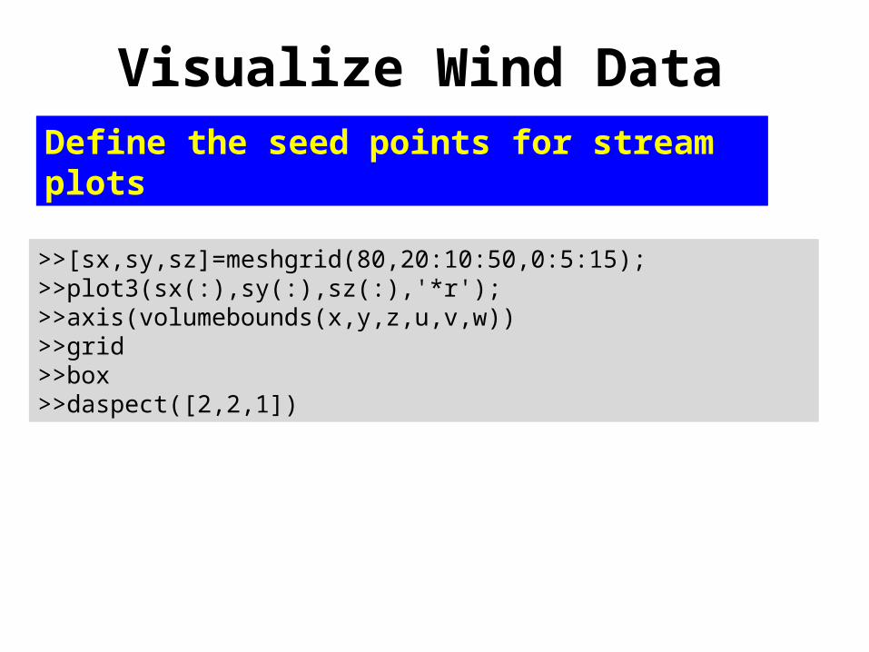
>>[sx,sy,sz]=meshgrid(80,20:10:50,0:5:15);>>plot3(sx(:),sy(:),sz(:),'*r');>>axis(volumebounds(x,y,z,u,v,w))>>grid>>box>>daspect([2,2,1])
Define the seed points for stream plots

Visualize Wind Data
streamline(x,y,z,u,v,w,sx(:),sy(:),sz(:))%streamline(X,Y,Z,U,V,W,startx,starty,startz)
“streamline.m” build-in
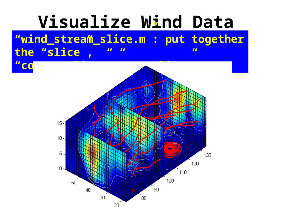
Visualize Wind Data“wind_stream_slice.m”: put together the “slice”, “contourslice”,”streamline”
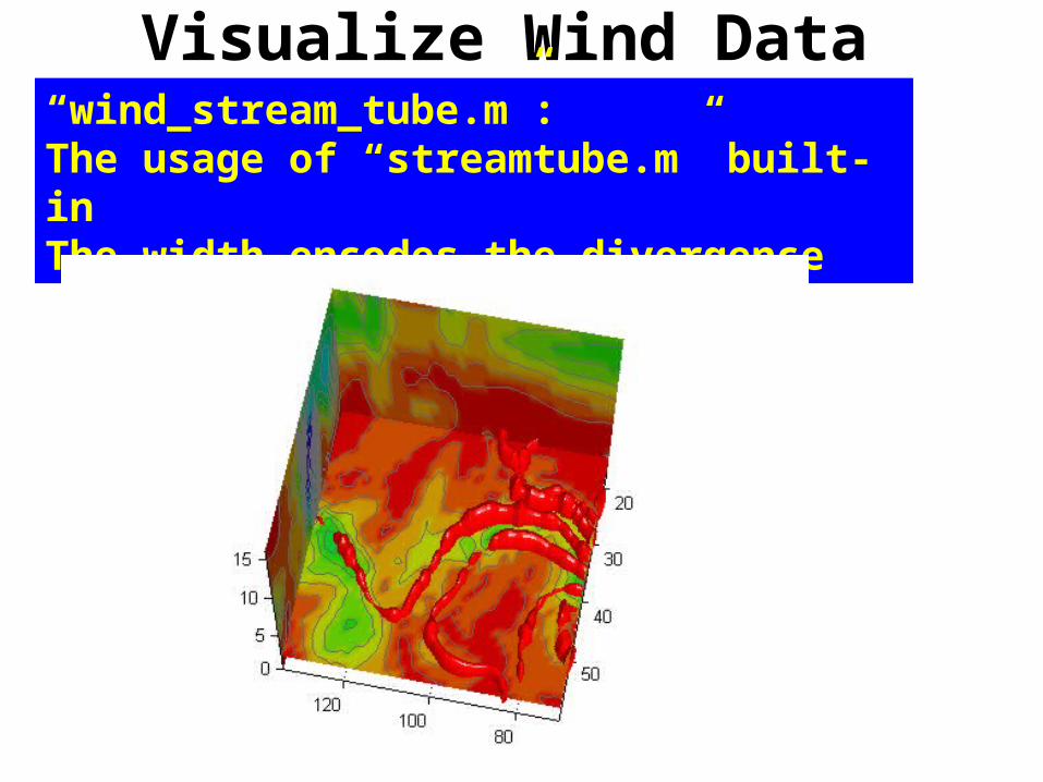
Visualize Wind Data“wind_stream_tube.m”: The usage of “streamtube.m” built-inThe width encodes the divergence
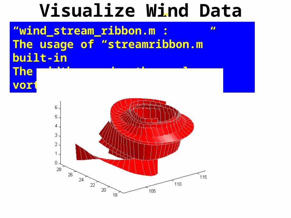
Visualize Wind Data“wind_stream_ribbon.m”: The usage of “streamribbon.m” built-inThe width encodes the curl or vorticity
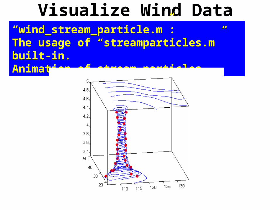
Visualize Wind Data“wind_stream_particle.m”: The usage of “streamparticles.m” built-in.Animation of stream particles
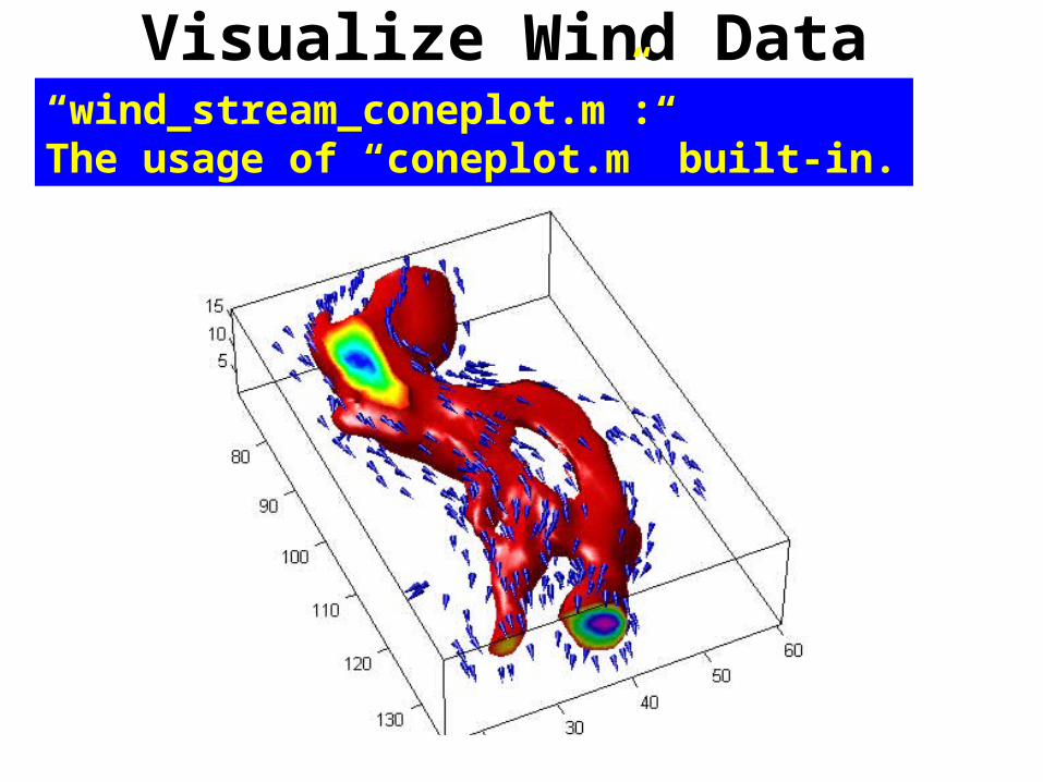
Visualize Wind Data“wind_stream_coneplot.m”: The usage of “coneplot.m” built-in.

The End