CENTRE FOR DYNAMIC MACROECONOMIC ANALYSIS

CONFERENCE PAPERS 2008

CASTLECLIFFE, SCHOOL OF ECONOMICS & FINANCE, UNIVERSITY OF ST ANDREWS, KY16 9AL

TEL: +44 (0)1334 462445 FAX: +44 (0)1334 462444 EMAIL: cdma@st-and.ac.uk

www.st-andrews.ac.uk/cdma

CDMC08/13

Estimating insurance and incentive effectsof labour market reforms

Andrey Launov*

University of WuerzburgAnd

UC Louvain-la-Neuve

Irene Schumm†

University of Wuerzburg

Klaus Wälde‡

UC Louvain-la-Neuve and University of Glasgow and CESifoJUNE 20, 2008 WORK IN PROGRESS

ABSTRACT

We formulate a general equilibrium matching model with spell-dependentunemployment benefits and endogenous search effort. The model gives rise to anendogenous distribution of unemployment duration characterized by a time-varying hazard function. Using methods from the literature on Semi-Markovprocesses, we obtain an expression for the aggregate unemployment rate underheterogeneous search effort. We perform structural estimation of the modelusing a German micro-data set (SOEP) and discuss the effects of the recentunemployment benefit reform (Hartz IV). Our results show that although thereform and economic growth have contributed to the reduction of the aggregateunemployment rate, aggregate welfare has gone down.JEL: J65, J64, C13Keywords: Search and Matching Model, Structural Estimation, UnemploymentInsurance

* Andrey Launov, Université catholique de Louvain à Louvain-La-Neuve, Place Montesquieu 3, 1348

Louvain-La-Neuve, Belgium, Phone: +32.10.47-4141, Email: andrey.launov@uni-wuerzburg.de.† Irene Schumm, University of Wuerzburg, Lehrstuhl fuer VWL II, Sandering 2, 97070 Wuerzburg,Phone: +49.931.31-2952, Email: irene.schumm@uni-wuerzburg.de.‡ Klaus Wälde, University of Glasgow, Department of Economics, Glasgow G12 8RT, Scotland,

Klaus@Waelde.com, www.waelde.com. Phone: +44.141.330-2446.

Estimating insurance and incentive e¤ectsof labour market reforms

Andrey Launov(a;b) , Irene Schumm(a) and Klaus Wälde(b;c); 1(a)University of Wuerzburg, (b)UC Louvain-la-Neuve, (c)University of Glasgow and CESifo

June 20, 2008work in progress

We formulate a general equilibrium matching model with spell-dependent unem-ployment bene�ts and endogenous search e¤ort. The model gives rise to an en-dogenous distribution of unemployment duration characterized by a time-varyinghazard function. Using methods from the literature on Semi-Markov processes,we obtain an expression for the aggregate unemployment rate under heteroge-neous search e¤ort. We perform structural estimation of the model using a Ger-man micro-data set (SOEP) and discuss the e¤ects of the recent unemploymentbene�t reform (Hartz IV). Our results show that although the reform and eco-nomic growth have contributed to the reduction of the aggregate unemploymentrate, aggregate welfare has gone down.

JEL Codes: J65, J64, C13Keywords: Search andMatching Model, Structural Estimation, Unemployment Insurance

1 Introduction

Continental European unemployment is notorious for its persistence. France, Italy and Ger-many have had rising unemployment rates from the 1960s up to 2000 and even onward. Thereseems to be a consensus now that a combination of shocks and institutional arrangementslies at the origin of these high unemployment rates (Ljungqvist and Sargent, 1998, 2007a,b; Mortensen and Pissarides, 1999; Blanchard and Wolfers, 2000). Neither institutions norshocks alone explain the rise in unemployment: institutions have always been there but un-employment has not (at least not at this level) and shocks have hit many countries but notall countries have high unemployment rates. The step from this shock-institutions insighttowards �nding a solution to the European unemployment problem seems to be short: As

1Contact details: Andrey Launov, Université catholique de Louvain à Louvain-La-Neuve, PlaceMontesquieu 3, 1348 Louvain-La-Neuve, Belgium, Phone: +32.10.47-4141, Email: andrey.launov@uni-wuerzburg.de. Irene Schumm, University of Wuerzburg, Lehrstuhl fuer VWL II, Sandering 2, 97070Wuerzburg, Phone: +49.931.31-2952, Email: irene.schumm@uni-wuerzburg.de. Klaus Wälde, Universityof Glasgow, Department of Economics, Glasgow G12 8RT, Scotland, Klaus@Waelde.com, www.waelde.com.Phone: +44.141.330-2446.

1

shocks will not go, we need to address the institutions. A common suggestion is to reducelong and generous unemployment bene�ts.Is this advisable? Should one reduce the length and level of unemployment bene�ts in or-

der to reduce unemployment? There is a classic e¢ ciency-equity trade-o¤ to be faced. Whilereducing unemployment per se is bene�cial, income of the unemployed and the insurancemechanism implicit in unemployment bene�ts should not be neglected.We examine qualitatively and quantitatively the employment and welfare e¤ects of a pol-

icy reform which reduces the length and level of unemployment bene�ts. We use Germanyas an example of a continental European country, as the so-called �Hartz IV reform�imple-mented in January 2005 comprises both the reduction of bene�ts and the cut of the durationof entitlement and because the German unemployment bene�t system has a typical two-tierstructure as in many other OECD countries. Unemployment insurance (UI) payments beforethe reform were paid for a period of 6 to 32 months followed by unemployment assistance(UA) payments, the latter potentially lasting up to in�nity. The experience of Germany withrising unemployment rates over decades is shared by many other countries and, similarly toGermany in 2005, many countries did reduce length and level of unemployment payments inorder to address the issue of high and persistent unemployment (OECD, 2004).The Hartz IV reform has introduced two main modi�cations. First, the UA payments,

formerly proportional to net earnings before the job loss, were replaced by a uniform bene�tlevel. The e¤ect of this new rule on the income of long-term unemployed workers wasambiguous. There were unemployed whose bene�t payments were lower before 2005 thanafter the reform, mainly unemployed workers from the low wage sector. Those were the�winners�of the reform (47 percent of long-term unemployed). On the other hand, therewere also long-term unemployed with relatively high wages before entering unemployment.These were a¤ected negatively by the new law and their income has dropped (53 percentof long-term unemployed). Despite the fraction of �winners�and �losers�is roughly equal,the gain of the winners has turned out to be lower than the loss of the losers leading to aloss of the average worker of a bit more than 7% due to Hartz IV (Blos and Rudolph, 2005;OECD, 2007). Second, for workers who entered unemployment from February 2006 onward,the maximum duration of entitlement to unemployment insurance payments was reduced to12 months (formerly, 15 months was the average).At �rst sight, the reforms seem to have worked. The reported unemployment rate dropped

between January 2005 and January 2007 from 12.3 to 10.2 percent. On the other hand,growth rates in Germany were (for German standards) fairly high. While the Germaneconomy shrank in 2003, it has recovered since then and probably also created new jobs.The real GDP grew by 0.8 percent in 2005 and by 2.9 percent in 2006. Given this background,we are left with at least three questions: Did the reform reduce unemployment and increaseoutput? (Yes.) Did it increase welfare of the unemployed and/or employed workers? (No.)Does it increase social welfare or expected utility? (No.) In short, our �ndings suggest thatpost-reform unemployment bene�ts reduced the insurance mechanism of UA payments toomuch and overemphasized the incentive e¤ect.2

We reach our conclusions by using a model which combines various strands of the litera-

2This does not mean that labour market institutions should not be reformed. It rather means that oneshould look for Pareto-improving reforms (e.g. introducing progressive social security payments).

2

ture and adds some new and essential features. We employ a general equilibrium matchingframework and extend the standard text-book model for time-dependent unemployment ben-e�ts, endogenous e¤ort, risk-averse households, an exogenous �residual search productivitye¤ect�and Semi-Markov tools. Each of these extensions is crucial. Unemployment bene�tsin our model need to depend on the length of the unemployment spell as this is a featureof basically all OECD unemployment bene�t systems. Letting agents optimally choose theire¤ort to �nd a job, we can analyze the incentive e¤ects of (reforms of) the unemploymentbene�t system on the search intensity. Risk-averse households are required as we also wantto evaluate insurance e¤ects. The residual e¤ect allows us to capture all e¤ects, other thanthe incentive e¤ect, that in�uence exit rates into employment. Finally, tools from the Semi-Markov literature are required as this allows us to deduce the aggregate unemployment ratefrom individual search. We can thereby compute macro e¢ ciency e¤ects resulting from microincentives.We solve this model numerically by looking at Bellman equations as di¤erential equa-

tions. This gives us solutions which are as accurate as numerical precision and which do notrequire us to approximate the model in any way. Optimal behaviour implies an exit rateinto employment which is a function of the time spent in unemployment. We thereby ob-tain a �exible enough endogenous distribution of unemployment duration which we employfor structural estimation of model parameters. Estimation by maximum likelihood is then(relatively) straightforward.The main theoretical contribution of our analysis is the explicit treatment of the Semi-

Markov nature of optimal individual behaviour due to the presence of spell-dependent un-employment bene�ts: Optimal exit rates not only depend on whether the individual isunemployed (the current state of the worker) but also on how long an individual has beenunemployed. While this Semi-Markov aspect has been known for a while, it has not beenfully exploited so far in the search literature. Using results from the applied mathematicsliterature, we obtain analytic expressions for individual employment probabilities contingenton current employment status and duration of unemployment. They allow us to computeaggregate unemployment rates using a law of large numbers in our pure idiosyncratic riskeconomy. Given this link from optimal individual behaviour to aggregate outcomes, we cananalyze the distribution and e¢ ciency e¤ects of changes in level and length of unemploymentbene�ts.The main empirical contribution is the careful modelling of exit rates into employment.

Individual incentives due to falling unemployment bene�ts imply more search e¤ort andtherefore higher exit rates over time. Empirical evidence shows, however, that exit rates tendto fall - at least after some initial increase over the �rst 3-4 months of unemployment. Wetherefore combine individual incentive e¤ects with an exogenous time-decreasing �residualsearch productivity e¤ect�which allows us to obtain - from a theoretical perspective - rising,falling and hump-shaped exit rates. Structural estimation then establishes that the modelcan replicate empirical stylized facts of �rst rising and then falling exit rates.The main policy contribution is our emphasis and structural estimation of the trade-o¤

between insurance and incentive e¤ects of labour market policies. The degree of risk-aversion- crucial for understanding the insurance e¤ect - is jointly estimated with exit rates andsearch productivity (and other model parameters). A comparative static analysis using theestimated version of the theoretical model then allows us to derive precise predictions about

3

the employment and distribution e¤ects of changes in the length and level of unemploymentbene�ts.Our paper is related to various strands in the literature. From a theoretical perspective,

we build on the search and matching framework of Diamond (1982), Mortensen (1982) andPissarides (1985), recently surveyed by Rogerson et al. (2005). Time-dependent unemploy-ment bene�ts and endogenous e¤ort have been originally analyzed by Mortensen (1977) ina one-sided job search model. Equilibrium search and matching models include Cahuc andLehman (2000), Fredriksson and Holmlund (2001) and Albrecht and Vroman (2005).3 Thesemodels, however, are less powerful than our model in explaining the anticipation e¤ect of thereduction in bene�ts, as exit rates within each bene�t regime are constant. There also existsa substantial literature that studies optimal insurance allowing for an arbitrary time path ofunemployment bene�t payments (Shavell and Weiss, 1979; Hopenhayn and Nicolini, 1997;Shimer and Werning, 2007). Our focus is more of a positive nature trying to understandthe welfare e¤ects of existing systems which have a simpler bene�t structure than the onesresulting from an opitmization approach. We also allow for an unlimited number of transi-tions between employment and unemployment and undertake a general equilibrium analysisas in Moscarini (2005).4

From an empirical perspective, we estimate a parametric duration model (Lancaster,1990) in which time dependence of the hazard function due to time-dependent bene�ts isfully described by the equilibrium solution of our theoretical model. Econometric modelswith time-dependent bene�ts were originally estimated by van den Berg (1990) and Ferrall(1997).5 Van den Berg et al. (2004) and Abbring et al. (2005) extend the setting byintroducing time dependence due to monitoring and sanctions. In contrast to our model,this literature deals with one-sided job search, which makes application of its estimates ina general equilibrium analysis rather di¢ cult. In addition to that, focus on the incentivee¤ect in is only partial (van den Berg et al., 2004; Abbring et al., 2005) and insurance e¤ectremains largely unaddressed. There also exists a larger empirical equilibrium search literaturethat deals with unemployment bene�t heterogeneity (Bontemps et al., 1999), heterogeneityin workers abilities (Postel-Vinay and Robin, 2002) and heterogeneity in workers value ofnonparticipation (Flinn, 2006). Unlike in our model, however, neither of these contributionsviews heterogeneity as being a result of time-dependence.Finally, Semi-Markov methods are taken from the applied mathematical literature, see

e.g. Kulkarni (1995) or Corradi et al. (2004).The structure of our paper is as follows. In section 2 we present the theoretical model,

institutional setting, behaviour of supply and demand sides and the combination of both ineconomic welfare. Section 3 describes the equilibrium properties of the model. Section 4illustrates the structural estimation and the underlying data. The simulation results and theevaluation of the institutions reforms are presented in section 5. Section 6 concludes.

3Coles and Masters (2007) also have time-dependent unemployment insurance but they do not analyze theimplications for individual e¤ort. Their focus is on a model with aggregate uncertainty implying stochasticseparation rates.

4Acemoglu and Shimer (1999) do consider a general equilibrium model, but their setting is restricted totime-invariant bene�ts only.

5See also Eckstein and van den Berg (2007) for literature review on nonstationary empirical models.

4

2 The model

We use a Diamond-Mortensen-Pissarides type matching model and extend it for time-dependent unemployment bene�ts, endogenous e¤ort, risk-averse households and an exoge-nous search productivity e¤ect. To solve it, we use Semi-Markov tools. The separation ratefor jobs is constant and there is no search on the job. We focus on steady states in ouranalysis.

2.1 Production, employment and labour income

The economy has a work force of exogenous constant size N: Employment is endogenousand given by L and the number of unemployed amounts to N � L: Firms produce underperfect competition on the goods market and each worker-�rm match produces output A,which is constant. The production process of the worker and the �rm can be interruptedby exogenous causes which occur according to a time-homogenous Poisson process with aconstant arrival rate �.Unemployed workers receive UI bene�ts b1 and UA bene�ts b2. Bene�ts are modelled to

re�ect institutional arrangements in many European countries. One of the most importantfeatures is the dependence of UI bene�ts on the unemployment spell. Empirical work hasrepeatedly shown (Mo¢ tt and Nicholson,1982; Blanchard and Wolfers, 2000) that the lengthof entitlement to unemployment insurance payments plays a crucial role in determining theunemployment rate. Workers with a spell s shorter than �s (say one year) receive UI bene�tsb1, afterwards, they receive b2,

b (s) =

�b1 0 � s � �sb2 �s < s

: (1)

We assume b1 > b2 � 0. Bene�ts can be paid either at a �xed level or proportional toprevious income.An unemployed worker �nds a job according to a time-inhomogenous Poisson process

with arrival rate � (:) : This rate will also be called the job-�nding rate, hazard rate or exitrate (into employment). We allow this rate to depend on e¤ort � (s (t)) an individual exertsto �nd a job. E¤ort today in t depends on the length s (t) this individual has been spendingin unemployment since his last job. The spell increases linearly in time and starts in t0where the individual has lost the job, i.e. s (t) = t � t0. An individual whose duration ofunemployment spell s (t) exceeds the length of entitlement to UI bene�ts �s (i.e. s (t) � t0+�s)will be called a long-term unemployed.In addition to individual e¤ort, the exit rate will also depend on aggregate labour market

conditions and on the �residual search productivity e¤ect�. Labour market conditions arecaptured by labour market tightness � that di¤ers across steady states, � � V=U . We assumethat e¤ort and tightness are multiplicative: no e¤ort implies permanent unemployment andno vacancies imply that any e¤ort is in vain. The residual e¤ect is a time (spell s) e¤ect andcaptures stigma, ranking (Blanchard and Diamond, 1994), unobserved productivity di¤eren-tials, changes in preferences and attitudes (frustration in search), loss in search productivity,etc., i.e. all e¤ects which imply that exit rates of long-term unemployed di¤er from exitrates of short-term unemployed. We denote this e¤ect by � (s) : While it can go either way,

5

empirically, we expect that productivity goes down, i.e. @� (s) =@s < 0: Hence, in full, theexit rate reads � (� (s (t)) �; � (s)).It is well-known (e.g. Ross, 1996, ch. 2) that the density of unemployment duration

when the exit rate is time-varying is given by

f (s) = � (� (s) �; � (s)) e�R s0 �(�(u)�;�(u))du: (2)

This density will be crucial later for various purposes including the estimation of modelparameters. It is endogenous to the model, as exit rate � (� (s (t)) �; � (s)) follows from theoptimizing behaviour of workers and �rms.6

Unemployment bene�ts are �nanced by a tax rate � on gross wages such that the netwage is w = (1� �)wgross. The budget constraint of the government therefore reads

�w

1� �L = b1Ushort + b2Ulong, (3)

where the number of short- and long-term unemployed adds to the total number of unem-ployed, Ushort+Ulong = N �L. The government adjusts the wage tax � such that this holdsat each point in time.The wage is determined by bargaining to which we return below.

2.2 Optimal behaviour

� Households

Households are in�nitely lived and do not save. The present value of having a job isgiven by V (w) and depends on the current endogenous wage w only. Employed workersenjoy instantaneous utility u (w; ) where captures disutility from working.7 The valueV (w) is constant in a steady state as the wage is constant, but di¤ers across steady states.Whenever a worker loses his job, he enters the unemployment bene�t system by obtaininginsurance payments b1 for the full length of �s. Workers are immediately granted full bene�tentitlements, i.e. unemployment payments are not experience rated. See the bargainingsetup for further discussion. Hence, the value of being unemployed when just having lost thejob is given by V (b1; 0) where 0 stands for a spell of length zero. This leads to a Bellmanequation for the employed worker of

�V (w) = u (w; ) + � [V (b1; 0)� V (w)] . (4)

The Bellman equation for the unemployed worker reads

�V (b (s) ; s) = max�(s)

�u (b (s) ; � (s)) +

dV (b (s) ; s)

ds+ � (� (s) �; s) [V (w)� V (b (s) ; s)]

�:

(5)The instantaneous utility �ow of being unemployed, �V (b (s) ; s) ; is given by three compo-nents. The �rst component shows the instantaneous utility resulting from consumption of

6Also note that due to drop of bene�ts at �s, f (s) will have a more general hurdle structure (see Appendix).7This parameter only serves to contrast search e¤ort of unemployed workers and plays no major role.

6

b (s) and e¤ort � (s). The second component is a deterministic change of V (b (s) ; s) as thevalue of being unemployed changes over time. The third component is a stochastic changethat occurs at job-�nding rate � (� (s) �; s) : When a job is found, an unemployed gains thedi¤erence between the value of being employed V (w) and V (b (s) ; s).An optimal choice of e¤ort � (s) for (5) requires

u�(s) (b (s) ; � (s)) + ��(s) (� (s) �; s) [V (w)� V (b (s) ; s)] = 0; (6)

where subscripts denote (partial) derivatives. It states that the expected utility loss resultingfrom increasing search e¤ort must be equal to expected utility gain due to higher e¤ort.We require that the value of unemployment an instant before becoming a long-term

unemployed is identical to the value of being long-term unemployed at �s, i.e.

V (b1; �s) = V (b2; �s) : (7)

� Firms

The value of a job J to a �rm is given by instantaneous pro�ts A � w= (1� �), whichis the di¤erence between revenue A and the gross wage w= (1� �), reduced by the risk ofbeing driven out of business

�J = A� w= (1� �)� �J , (8)

where � stands for the interest rate (being identical to the discount rate of households).Given that individual arrival rates are a functions of the individual unemployment spell,

the expected rate of exit out of unemployment is just the mean over individual arrival rates,given the endogenous distribution of the unemployment spell f (s) from (2),

�� =

Z 1

0

� (� (s) �; � (s)) f (s) ds. (9)

As a consequence, the vacancy �lling rate is � (t) � ��1��: The value of a vacant job is�J0 = � + � (t) [J � J0] : With free entry, the value of holding a vacancy is J0 = 0, leadingto

J = �=��. (10)

� Wages

We let wages be determined by Nash bargaining. We assume that the outcome of thebargaining process is such that workers receive a share � of the total surplus of a successfulmatch V (w)�V (b1; 0) = �

�J�w1���� J0 + V (w)� V (b1; 0)

�. The total surplus is the gain

of the �rm plus the gain of the worker from the match where the latter crucially on theoutside option of the worker. The fact that we use V (b1; 0) as the outside option of theworker means that all workers (even if only working for an instant or, in the limit, if onlybargaining) are entitled to full unemployment bene�ts, i.e. b1 over the full length �s and b2for s > �s. An alternative would consist in specifying V (b (s) ; s) as the outside option: if thebargain fails, the unemployed worker remains unemployed and continues to receive bene�ts

7

she received before the unsuccessful bargaining. This would be theoretically interesting asan endogenous wage distribution would arise (see Albrecht and Vroman, 2005) where thedistinguishing determinant across workers is the previous unemployment spell. Using anidentical outside option for all individuals, however, has the advantage that we stay in aSemi-Markovian framework. Once an unemployed �nds a job, all history is deleted, allworkers are the same and, independently of their employment history, earn the same wage.History only matters if one day she should lose her job again.8

Following the steps as in Pissarides (1985), we end up with a generalized wage equationthat reads (see app. B.6)

(1� �)u (w) + �w

1� �= (1� �)u (b1; � (0)) + � [A+ � ] . (11)

The left hand side corresponds to what in models with risk-neutrality and without taxationis simply the wage rate. So, with u (w) = w and � = 0 we would obtain just w on the left.The tax rate, that appears as the term w= (1� �), results from the instantaneous pro�t ofa �rm (8) which needs to pay a gross wage of w= (1� �). The right hand side is a simplegeneralization of the standard wage equation of Pissarides (1985). Instead of bene�ts forthe unemployed (which we would �nd on the right for risk-neutral households and no time-dependence of e¤ort), we have instantaneous utility from being unemployed. The impact ofthe production side is unchanged when compared to the standard wage equation.Instead of specifying the outside option di¤erently, one could also allow for strategic bar-

gaining. Many recent papers have used strategic bargaining given that either payo¤s changeover time and Nash bargaining would correspond to myopic behaviour (Coles and Wright,1998; Coles and Muthoo, 2003), that a careful analysis of on-the-job search makes strategicbargaining more appropriate (Cahuc, Postel-Vinay and Robin, 2006) or that unemploymentdoes not have such a strong e¤ect on bargaining as generally thought (Hall and Milgrom,2008).9 Given that we want to focus here on the direct incentive e¤ects of non-stationaryunemployment bene�ts on search e¤ort, we �switch o¤�the strategic channel and leave thisfor future work.

2.3 Welfare

When we evaluate unemployment policies, we take all agents in our economy into account.There are workers with value V (w) ; the unemployed with value V (b (s) ; s) depending ontheir spell s and �rms with value J:When we want to compare one policy to another, we lookat output, employment, individual e¤ects and overall welfare. We obtain a social welfarefunction by aggregating - in spirit as in Hosios (1990) - over all these welfare levels in a

8Our assumption that all workers, even if they have worked only for a second, are entitled to b1 for the fullperiod of length �s is identical to saying that bene�t payments are not experience rated. While the absence ofexperience rating is generally distorting the �rms decision to lay o¤workers (see e.g. Mongrain and Roberts,2005), this does not play a role in our setup as the separation rate is exogenous. It would be interesting tostudy the impact of endogenous separation decisions but we leave this for future research.

9Coles and Masters (2004) analyse wage setting by strategic bargaining in a matching setup with non-stationary unemployment bene�ts. They do not consider endogenous search intensity, however.

8

standard Bentham-type utilitarian way,10

= L [V (w) + J ] + (N � L)

�Z �s

0

V (b1; s) f (s) ds+

Z 1

�s

V (b2; s) f (s) ds

�: (12)

Social welfare is given by the number L of employed workers/ �rms times their welfare plusthe number of unemployed workers N �L times the average welfare of an unemployed. Thisaverage is obtained by integrating over all spells s, where f (s) is the endogenous density(2), with exit rates � (� (s) �; � (s)) that follow from the steady state solution of the model,and the V (bi; s) are the values of being unemployed with a spell s and bene�t payments bifrom (1).

3 Equilibrium properties

3.1 Individual (un)employment probabilities

In models with constant job-�nding and separation rates, the unemployment rate can easilybe derived by assuming that a law of large numbers holds. Aggregate employment dynamicscan then be described by _L = � [N � L]��L which allows to compute unemployment rates.With spell-dependent e¤ort, individual arrival rates � (:) are heterogeneous and employmentdynamics need to be derived using techniques from the literature on Semi-Markov or renewalprocesses, e.g. Kulkarni (1995) or Corradi et al. (2004).The generalization of Semi-Markov processes compared to continuous time Markov chains

consists in allowing the transition rate from one state to another to depend on the time anindividual has spent in the current state. We apply this here and let the transition rate fromunemployment to employment depend on the time s the individual has been unemployed.Hence, switching from a constant job-�nding rate � to a spell-dependent rate � (s) impliesswitching fromMarkov to Semi-Markov processes. Processes are called �semi�as the history-dependence of the job �nding rate � (s) is not Markov. Processes are still called �Markov�asonce an individual has found a job, history no longer counts. This is also why these processesare called renewal processes: whenever a transition to a new state occurs, the system startsfrom the scratch, it is �renewed�and history vanishes.We start by looking at individual employment probabilities. Let pij (� ; s (t)) describe

the probability with which an individual, who is in state i (either e for employed or u forunemployed) today in t, will be in state j 2 fe; ug at some future point in time � , given thathis current spell is now s (t). These expressions read, starting with s (t) = 0 and taking intoaccount that the separation rate � remains constant (see app. A.3),

puu (� ; 0) = e�R �t �(s(y))dy +

Z �

t

e�R vt �(s(y))dy� (s (v)) peu (� � v) dv; (13a)

peu (�) =

Z �

t

e��[v�t]�puu (� � v; 0) dv: (13b)

10Dividing by N gives expected utility of a worker �thrown into� this economy from behind some �veilof ignorance�. Higher social welfare is therefore identical to higher expected utility. One could thereforeequilvalently ask in which economy such a worker would like to land.

9

Expressions for complementary transitions are given by pue (�) = 1 � puu (�) and pee (�) =1� peu (�), respectively.These equations have a straightforward intuitive meaning. Consider �rst the case of �

being not very far in the future. Then all integrals (for � = t) are zero and the probabilityof being unemployed at � is, if unemployed at t; one from (13a) and, if employed at t, zerofrom (13b). For a � > t; the part e�

R �t �(s(y))dy in (13a) gives the probability of remaining in

unemployment for the entire period from t to � : An individual unemployed today can alsobe unemployed in the future if he remains unemployed from t to v (the probability of whichis e�

R vt �(s(y))dy), loses the job in v (which requires multiplication with the exit rate � (s (v)))

and then moves from employment to unemployment again over the remaining interval � � v(for which the probability is peu (� � v)). As this path is possible for any v between t and� ; the densities for these paths are integrated. The sum of the probability of remainingunemployed all of the time and of �nding a job at some v but being unemployed again at� gives then the overall probability puu (� ; 0) of having no job in � when having no job in t:Note that there can be an arbitrary number of transitions in and out of employment betweenv and � : The interpretation of (13b) is similar. The probability of remaining employed fromt to v is simpler, e��[v�t]; as the separation rate � is constant.As we can see, these equations are interdependent: The equation for puu (�) depends on

peu (� � v) and the equation for peu (�), in turn, depends on puu (� � v). Formally speaking,these equations are integral equations, sometimes called Volterra equations of the �rst type(13b) and of the second type (13a). Integral equations can sometimes be transformed intodi¤erential equations, which will simplify their solution in practice. In our case, however, notransformation into di¤erential equations is known.After having computed the probability of being unemployed in � when being unemployed

in t for individuals that just became unemployed in t, i.e. who have a spell of lengths (t) = 0; we will need an expression for puu (� ; s (t)). This means, we will need the transitionprobabilities for individuals with an arbitrary spell s (t) of unemployment. Luckily, giventhe results from (13a and b), this probability is straightforwardly given by

puu (� ; s (t)) = e�R �t �(s(y))dy +

Z �

t

e�R vt �(s(y))dy� (s (v)) peu (� � v) dv: (14)

An unemployed with spell s (t) in t has di¤erent exit rates � (s (y)) which, however, are knownfrom our analysis of optimal behaviour at the individual level. Hence, only the integrals in(14) are di¤erent, the probabilities peu (� � v) can be taken from the solution of (13a and b).

3.2 Aggregate unemployment

Given our �nding in (13) and (14) on peu (�) and puu (� ; s (t)), we can now compute theexpected number of unemployed for any distribution of spell F (s),

Et [N � L� ] = [N � Lt]

Z 1

0

puu (� ; s (t)) dF (s (t)) + peu (�)Lt: (15)

Starting at the end of this equation, given there are Lt employed workers in t, the expectednumber of unemployed workers at some future point � out of the group of those currently

10

employed in t is given by peu (�)Lt: Again, one should keep in mind that the probabilitypeu (�) allows for an arbitrary number of switches between employment and unemploymentbetween t and � ; i.e. it takes the permanent turnover into account.For the unemployed, we compute the mean over all probabilities of being unemployed in

the future, if unemployed today, by integrating over puu (� ; s (t)) given the current distrib-ution F (s (t)) : Multiplying this by the number of unemployed today, N � Lt, gives us theexpected number of unemployed at � out of the pool of unemployed in t. The sum these twoexpected quantities gives the expected number of unemployed at some future point � :The expected unemployment rate at � is simply the expression (15) divided by N:When

we focus on a steady state, we let � approach in�nity. In order to obtain a simple ex-pression for the aggregate unemployment rate and to show the link to the textbook ex-pression, we assume a pure idiosyncratic risk model where micro-uncertainty cancels out atthe aggregate level. Hence, we assume a law of large numbers holds and the populationshare of unemployed workers equals the average individual probability of being unemployed.This �removes�the expectations operators, so that (15) for a steady state becomes N � L= [N � L]

R10puu (s (t)) dF (s (t))+ peuL:We have replaced L� = Lt by the steady state em-

ployment level L and the individual probabilities by the steady state expressions puu (s (t))and peu: The probability peu is no longer a function of � as this probability will not changein steady state, while there will always be a distribution of puu (s), even in steady state.Solving for the unemployment rates gives

U

N=

peu

peu +�1�

R10puu (s (t)) dF (s (t))

� = peupeu +

R10pue (s (t)) dF (s (t))

; (16)

where the second expression is more parsimonious. If we assumed a constant job arrivalrate here, we would get peu = puu = �= (�+ �) and pue = �= (�+ �). Inserting this intoour steady state results would yield the standard expression for the unemployment rate,U=N = �= (�+ �). In our generalized setup, the long-run unemployment rate is given bythe ratio of individual probability peu to be unemployed when employed today divided bythis same probability plus 1�

R10puu (s (t)) dF (s (t)).

3.3 Functional forms and steady state

For estimation purposes and for the numerical solution, we need functional forms for theinstantaneous utility function and for the arrival rate. We assume that the instantaneousutility function of an unemployed worker used e.g. in (5) is

u (b (s) ; � (s)) =b (s)1��

1� �� � (s) . (17)

E¤ort is measured in utility terms. The utility function of an employed worker has the samestructure only that consumption is given by w and e¤ort is the constant .The arrival rate of jobs � (� (s) �; � (s)) is assumed to obey

� (� (s) �; � (s)) = � (s) [� (s) �]� , with � (s) = �1e��i[s��s] + �2: (18)

If one interprets � (s) as a productivity of search, one can look at the expression for � (:) likeat a production function. Input factors are e¤ort � (s) and vacancies per unemployed worker

11

�. With 0 < � < 1, inputs have decreasing returns. E¤ort � (s) follows from behaviourof households and labour market tightness � is the result of free entry and exit into thecreation of vacancies. Search productivity is an exogenous function of the unemploymentspell s: For estimation purposes below, we allow the productivity e¤ect to change at di¤erent(depreciation) rates �i; depending on whether individuals receive UI payments b1 or UApayments b2. We also allow parameters to take any sign in the estimation procedure. Froma theoretical perspective, however, we would expect all parameters �i and �i to be positive.This would imply that the productivity falls in the spell s and approaches the constant �2 > 0.For a worker who has just lost his job, it is higher and given by � (s) = �1e

�i�s + �2 > �2.Note that even if depreciation rates di¤er from the UI to the UA phase, search productivityis continuous at �s and given by �1 + �2:In a steady state, all aggregate variables are constant and there will be a stationary

distribution for unemployment spells. The solution of the steady can most easily be foundin two steps. Taking the wage w and labour market tightness � as exogenous, one can useexpressions related to the unemployed for e¤ort, the value of being unemployed and thevalue of a job, � (b (s) ; s), V (b (s) ; s) and V (w) : Once these quantities are known, one canuse the remaining equations of the model to solve for the wage rate and tightness, w and�. In doing so, all other endogenous variables (exit rate � (s) and the implied density f (s) ;instantaneous utilities u (:), the tax rate �; individual employment probabilities pij and theimplied number of short- and long-term unemployed and the unemployment rate U=N , thenumber of vacancies, the value function J for the �rm and social welfare ) are determinedas well. Appendix A.2 provides an explicit presentation of all equations (which above in themodel description are given implicitly) and describes the solution procedure.

4 Structural estimation

4.1 Stylized facts

The model is estimated using the data from the German Socio-Economic Panel (GSOEP).11

Before we do so, we would like to see whether it is able to match central stylized facts.As our focus is on the exit rates, which are key to understanding incentives resulting fromchanges in unemployment bene�ts, we need to make sure that our model is �exible enoughto replicate the most important features of exit behaviour observed in the data. Thesefeatures are shown in Figure 2.The left panel of Figure 2 plots a non-parametric estimate of the hazard function for the

entire sample of unemployment durations.12 This non-parametric hazard has a clear non-monotonic behaviour. Ups and downs are induced by multiplicity of entitlement lengths �sand peaks largely correspond to each and every value of �s, i.e. the time point at which bene�tsdrop. This is further con�rmed by the estimated non-parametric hazard for a subsample ofindividuals with �s = 12 (which is the case for approx. 50% of our observations) shown in

11GSOEP is a panel survey of individuals held on the annual basis by the Deutsche Institut für Wirtschafts-forschung (Berlin). See Appendix for more information about the data.12See Tanner and Wong (1983) for the de�nition of the estimator and consistency proof. We use Gaussian

kernel. Optimal bandwith is estimated by cross-validation discussed in Tanner and Wong (1984).

12

the right panel.

Figure 1 Non-parametric hazard functions and model predictions

Thus the individual exit rate derived from the theoretical model must have at leasttwo characteristics, namely: a) steady increase before the expiration of entitlement (as inMortensen, 1977), and b) steady decrease thereafter (as in Heckman and Borjas, 1980). Ourtheoretical exit rates are broadly consistent with both. When we assume that there is noe¤ect other than that of bene�ts and tightness, i.e. � (s) is constant in (18) due to �j = 0 (nostigma), our model predicts exit rates that increase before �s. If �j is very high, exit rates fallover time. For intermediate values of �j, we get a non-monotonic behaviour and exit ratesincrease before �s and fall subsequently, featuring peak at �s. We are therefore con�dent thatour theoretical exit rates are su¢ ciently �exible for a successful estimation of the model.

4.2 Econometric model

� Speci�cation

Estimation of model parameters uses a part of the numerical solution method for thesteady state. As described in app. A.2, for a given wage w and vacency to unemploymentratio �; individual e¤ort over the unemployment spell can be computed. Using individualsurvey data implies that the wage w for each individual is known and the corresponding � canbe taken frommacro data. Individual e¤ort can therefore be computed and model parameterscan be estimated without specifying the wage setting mechanism. If we used linked employer-employee data, the model could be estimated by using the observable productivity data.This would allow us to estimate the bargaining power parameter � as well. For the restof the parameters unrelated to wage setting mechanism, however, both approaches must beequivalent (assuming that wage setting in the second one is correctly speci�ed). Further,computing the steady state solution suggests that estimation with given wage and tightnessis faster by a factor of at least 4 or 5.Computing individual e¤ort simultaneously provides exit rates �1 (si; �) and �2 (si; �),

i.e. before and after expiration of entitlement respectively. Since the data are sampled asa �ow of entrants into unemployment and employment, exit rates contain all information

13

necessary for the construction of the likelihood function. Our data consist of three types ofunemployed individuals:

a) Individuals who enter unemployment with the right to claim unemployment insurance(UI) bene�ts and exit unemployment before the expiration of entitlement period

b) Individuals who enter unemployment with the right to claim UI bene�ts, fail to �nd a jobbefore entitlement expires, transit to a lower unemployment assistance (UA) bene�tsand exit unemployment (or not) only after the expiration entitlement

c) Individuals who do not have the right to claim UI bene�ts and enter unemploymentreceiving lower UA bene�ts from the very beginning (if at all)

Let � denote the vector of parameters to estimate, i.e. � =��; �; �; �j; �j

j=1;2

.13 Fur-thermore let li de�ne the length of previous/current individual job. Keeping in mind thatjob loss is governed by a homogeneous Poisson process with rate �, which implies exponen-tial distribution of the length of the job spell, we get the following log-contributions for theabove types of individuals

a)ln `i (�) = dj;i ln�� �li + du;i ln�1 (si; �)�Z si

0

�1 (u; �) du (19a)

b)ln `i (�) = dj;i ln�� �li

�Z �si

0

�1 (u; �) du+ du;i ln�2 (si; �)�Z si

�si

�2 (u; �) du (19b)

c)ln `i (�) = dj;i ln�� �li + du;i ln�2 (si; �)�Z si

0

�2 (u; �) du, (19c)

where du;i is an indicator variable such that du;i = 1 if unemployment spell is uncensoredand dj;i is an indicator variable such that dj;i = 1 if job spell is uncensored. Finally, thelog-contribution of entrants to employment is simply

ln `i (�) = dj;i ln�� �li (19d)

� Identi�cation

Absence of analytical solutions for the structural exit rates �1 (si; �) and �2 (si; �) preventsus from obtaining any analytical result on the identi�ability of a general model describedby � as above. However, even a medium size numerical analysis shows that the modelwhich allows both � and � vary free is not identi�able. This holds for di¤erent shapes ofnon-bene�t e¤ect, including the constant one. Therefore we are to consider two di¤erentlines of speci�cation,

(i): � = 1=2, 0 < � < 1 and(ii): 0 < � < 1, � = 1=2,

the rest being equal.

13As typical for the majority of empirical search models, we impose � exogenously. The rate of timepreference is set to 0:003, which corresponds to annual rate of 3:7%.

14

As to the rest of the parameters, � is always identi�ed from job duration data. Given the�xed residual e¤ect, � in (i) and � in (ii) are always identi�ed as unique shape parameters ofthe hazard function. Introduction of a time dependent residual e¤ect implies identi�cationbounds for � and � which will depend on the shape of � (s). Finally, even if identi�able underfairly general forms of � (s), the more parsimonious the speci�cation of � (s) is, the better isthe numerical performance of the model. Extensive exploratory analysis of functional formsfor � (s) has led us to the following choices

(i) : � (s) = ��1 + e��s

�, 8s (20)

(ii) : � (s) =

�2�, s � �s��1 + e��[(s��s)]

�, s > �s

(21)

These choices insure well-behaved and at the same time best �tting models. All otherextensions of (20)-(21) either converge to the above forms or fail. It is to be noted, however,that the best shape of the residual e¤ect is a purely data-speci�c issue and so should di¤eron a case by case basis.

4.3 Estimation results

� Model selection

Given the above discussion we estimate three di¤erent models. Model 1 is the baselinemodel with � = 1=2, and constant �, which assumes pure bene�t/tightness e¤ect. Model 2is the model with unrestricted � and the residual e¤ect as in (20). Model 3 is a model withunrestricted � and the residual e¤ect as in (21).

Model 1 Model 2 Model 3Param. Coe¤. p-Value Coe¤. p-Value Coe¤. p-Value

� 0.0140 0.0000� 0.0141 0.0000� 0.0142 0.0000�

� 0.1507 0.1249 0.1835 0.0774� 0.0085 0.0165� 0.0053 0.0128� 0.0422 0.0000�

� 0.0571 0.0000� 0.0983 0.0432�

� 0.1904 0.0224�

log-L - 3187.278 - 3171.318 -3162.242

� denotes signi�cance at 5% level, p-Values for one-sided test Ha : �k > 0

Speci�cation Model selection� � � (s) Test p-Value

M 1 0:5 free � 2 vs 1 LRT: �2(1) 0.0000M 2 0:5 free �

�1 + e��s

�3 vs 2 Vuong �89 0.0554

M 3 free 0:5

�2� s � �s��1 + e��[s��s]

�s > �s

Table 1 Estimation results

15

Estimation results for all models are reported in Table 1. The corresponding hazard ratespredicted for an individual with average sample characteristics and average entitlement rightare plotted in �g. 2.The very �rst question we ask is that of model selection. The results of the relevant

model selection tests are reported below Table 1. First of all, we recognize that Model 1is nested in Model 2, so standard LR test applies. From the model selection summary wesee that the baseline model is clearly rejected in favour of Model 2. The speci�cations withrestricted � and �, to the contrary, are non-nested. Looking at the values of log-likelihood,we can see that any information criterion will speak in favour of Model 3. In addition weperform a Vuong (1989) test for non-nested models. Its results show that on 10% signi�cancelevel Model 3 is closer to the true model than Model 2. Taken together, these evidence makeus stop our choice on Model 3.We also see that the hazard rate implied by the best speci�cation (violet line in �g. 2)

repeats the monotonicity pattern of the nonparametric estimates in the discussion of thestylized facts.

Figure 2 Predicted hazard functions

� Preliminary discussion

As for the estimation results alone, our main �nding is the signi�cance of � (see Table1, Model 3; this result is true for both one-sided and two-sided alternatives). This meansthat changes in optimal e¤ort in response to any unemployment bene�t reform, be it thereform of b or of �s, will have a signi�cant impact on the exit rate out of unemployment.This �nding in particular can clarify the empirical dispute about the dependence betweenunemployment bene�ts and exit decision. Evidence in the literature are con�icting withHujer and Schneider (1989) and Arulampalam and Stewart (1995) �nding minor no negligibledependence and Carling et al. (2001) and Røed and Zhang (2003) stating the opposite.Despite we do not rule out that for certain types of heterogeneous agents the change in

16

bene�ts may play no role, our above result shows that in aggregate terms there exists apositive signi�cant relationship between the reemployment risk and any change in the level ofunemployment bene�t payments. Consequently, any change in the design of unemploymentbene�t mechanism will induce a signi�cant response on the macro level.

� Predicting labour productivity A and vacancy cost

After having estimated �; �; �, �i and �i, we are left with determining A and : Thewage w and tightness � were taken as exogenous in this �rst part of the estimation whichwas built on the household side of the model only. As the wage and tightness are endogenousin general equilibrium, we now take the estimated parameters � and compute parameters Aand using the full general equilibrium structure of our economy in the steady state (seesect. 3.3). We compute A and such that the average wage and average tightness in oursample result as general equilibrium endogenous variables in our model.

5 The e¤ects of labour market reforms

In this chapter we use the structurally estimated parameters in order to describe the steadystate equilibrium of 2004 and to evaluate the reform e¤ective as of January 2005. We basethe simulations on the parameters of model 3 where � is set to 0:5.

5.1 The pre-reform steady state

All parameters plus some selected endogenous variables are provided in tab. 2. The rate oftime preference � is chosen to match the annual interest rate of 3:7 percent. The bargainingpower � is set equal to :5: In the pre-reform steady state, bene�t payments of both short-termand long-term unemployed workers depend on the previous wage. The replacement rates aregiven by bi=w and are sample means for those entitled to UI and UA payments. These ratiosare pretty close to statutory replacement rates. Average sample entitlement to UI paymentsis 15 months, again for those entitled to UI payments. Our estimation procedure implies adegree of risk aversion �; separation rate �, search productivity �; depreciation rate � ande¤ort elasticity �: Labour productivity of A is just above the endogenous wage rate of 2250DM (German marks), leaving the di¤erence for �rms to pay for vacancy costs : Comparingour tax rate � and unemployment rate u to actual social security contribution rate (this isthe only purpose of taxes in our model) of 0:06 and the actual unemployment rate of 0:12,our model �ts real data very well.For comparative statics below, we will take the exogenous parameters, the estimated and

the predicted parameters as given. We will then change policy parameters to understandthe e¤ects on equilibrium values.

17

exogenous parameters� � �.003 .5 .5

estimated and predicted parameters� � � �

.014 .042 .098 .190A ��

2432 72.9policy parameters

b1w

b2w

�s.6 .53 15

equilibrium valuesw u � �

2250 DM 11.9% .3 7.3%

Table 2 Parameter and selected equilibrium values (see text above for details)

Although the economy is in the steady state, there are still dynamics on the micro level.At any point in time individuals �nd and lose jobs. Once unemployed, the closer expirationof the entitlement to UI bene�ts is, the harder they try to �nd a job. In addition to that,unemployed workers lose search productivity over the unemployment spell. So the exit ratethat describes the steady state distribution of unemployment spells is in�uenced by all thesefactors. Figure 4 illustrates the developments on the micro level. E¤ort in the right upperpanel expressed in consumption is equivalent to consumption loss ranging from 12 to 21percent.14

0 20 40 60 800.04

0.05

0.06

0.07

0.08

0.09

es timated produc tiv ity0 20 40 60 80

4

5

6

7

8

ef f ort

0 10 20 300.05

0.06

0.07

0.08

0.09

0.1

ex it rate0 10 20 30

2.97

2.98

2.99

3

3.01x  10

4

value of  unemployment

Figure 3 Productivity, e¤ort, exit rate and value of being unemployed over time

14Share of consumption x lost due to search is determined by ([1� x] b (s))1�� = (1� �) =

b (s)1��

= (1� �)� � (s).

18

5.2 Benchmarks

Before we undertake policy simulations, we need some benchmarks to evaluate whether themodel does a good job at replicating data (beyond micro behaviour) and what to expectfrom a quantitative perspective.

� Some facts about Germany

The central quantity against which we evaluate the macroeconomic performance of ourmodel is the unemployment rate. From January 2005 to January 2007 it fell from 12.3% to10.2%. Can our model, taking the labour market reforms and economic growth in Germanyinto account, explain this drop in unemployment? When undertaking comparative static, wewill also exogenously increase labour productivity A such that it re�ects economic growth inGermany. Real GDP in Germany grew by 0.8 percent in 2005 and by 2.9 percent in 2006.One can evaluate the model performance also against other time trends. For example,

unemployment insurance contributions, which correspond to the tax rate in our model,were reduced from 6.5% to 4.2%. The real gross wage reduced by unemployment insurancecontributions stayed basically constant over this period. The number of vacancies more thandoubled from 268,296 to 593,667.15 Evaluating the impact on the value of the �rm J wouldalso be interesting but no appropriate data has been found so far.

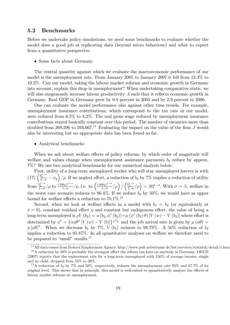
� Analytical benchmarks

When we ask about welfare e¤ects of policy reforms, by which order of magnitude willwelfare and values change when unemployment assistance payments b2 reduce by approx.7%? We use two analytical benchmarks for our numerical analysis below.First, utility of a long-term unemployed worker who will stay unemployed forever is with

(17)�b1��2

1�� � �2

�=�: If we neglect e¤ort, a reduction of b2 by 7% implies a reduction of utility

from b1��2

1�� =� to(:93b2)

1��

1�� =�; i.e. to�(:93b2)

1��

1�� =��=�b1��2

1�� =��= :931��:With � = :5; welfare in

the worst case scenario reduces to 96:4%: If we reduce b2 by 50%, we would have as upperbound for welfare e¤ects a reduction to 70:1%:16

Second, when we look at welfare e¤ects in a model with b1 = b2 (or equivalently at�s = 0), constant residual e¤ect � and constant but endogenous e¤ort, the value of being along-term unemployed is �V (b2) = u (b2; �

� (b2))+� (�� (b2) �) [V (w)� V (b2)] where e¤ort is

determined by �� = f���� [V (w)� V (b)]g1

1�� and the job arrival rate is given by � (��) =� [��]�. When we decrease b2 by 7%; V (b2) reduces to 98:79%. A 50% reduction of b2implies a reduction to 95:87%. In all quantitative analyses on welfare we therefore need tobe prepared to �small�results.17

15All data comes from Federal Employment Agency, http://www.pub.arbeitsamt.de/hst/services/statistik/detail/z.html16A reduction by 50% is probably the strongest e¤ect the reform can have on anybody in Germany. OECD

(2007) reports that the replacement rate for a long-term unemployed with 150% of average income, singleand no child, dropped from 55% to 26%.17A reduction of b2 by 7% and 50%, respectively, reduces the unemployment rate 95% and 87.7% of its

original level. This shows that in principle, this model is well-suited to quantitatively analyse the e¤ects oflabour market reforms on unemployment.

19

5.3 Policy modelling

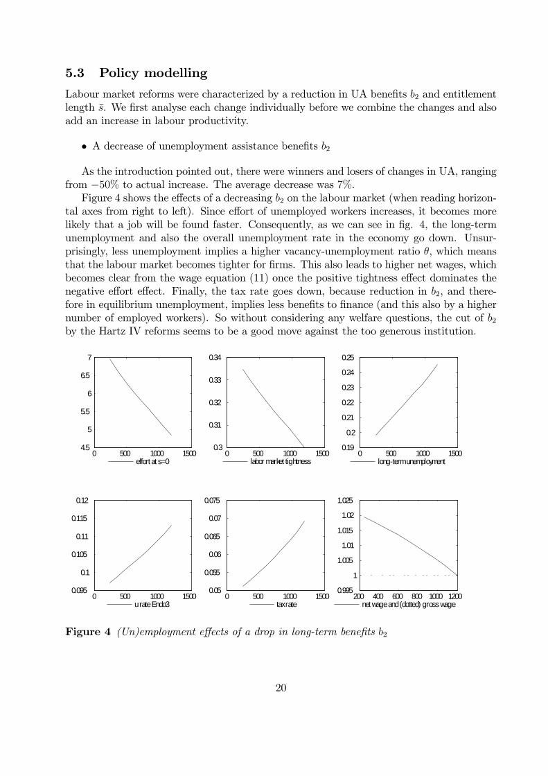
Labour market reforms were characterized by a reduction in UA bene�ts b2 and entitlementlength �s. We �rst analyse each change individually before we combine the changes and alsoadd an increase in labour productivity.

� A decrease of unemployment assistance bene�ts b2

As the introduction pointed out, there were winners and losers of changes in UA, rangingfrom �50% to actual increase. The average decrease was 7%:Figure 4 shows the e¤ects of a decreasing b2 on the labour market (when reading horizon-

tal axes from right to left). Since e¤ort of unemployed workers increases, it becomes morelikely that a job will be found faster. Consequently, as we can see in �g. 4, the long-termunemployment and also the overall unemployment rate in the economy go down. Unsur-prisingly, less unemployment implies a higher vacancy-unemployment ratio �, which meansthat the labour market becomes tighter for �rms. This also leads to higher net wages, whichbecomes clear from the wage equation (11) once the positive tightness e¤ect dominates thenegative e¤ort e¤ect. Finally, the tax rate goes down, because reduction in b2, and there-fore in equilibrium unemployment, implies less bene�ts to �nance (and this also by a highernumber of employed workers). So without considering any welfare questions, the cut of b2by the Hartz IV reforms seems to be a good move against the too generous institution.

200 400 600 800 1000 12000.995

1

1.005

1.01

1.015

1.02

1.025

net wage and (dotted) gross wage

0 500 1000 15000.3

0.31

0.32

0.33

0.34

labor market tightness0 500 1000 1500

0.19

0.2

0.21

0.22

0.23

0.24

0.25

long­term unemployment

0 500 1000 15000.05

0.055

0.06

0.065

0.07

0.075

tax rate

0 500 1000 15004.5

5

5.5

6

6.5

7

effort at s=0

0 500 1000 15000.095

0.1

0.105

0.11

0.115

0.12

u rate Endo3

Figure 4 (Un)employment e¤ects of a drop in long-term bene�ts b2

20

When we add welfare measures in �g. 5, however, the unambiguously positive impressionof the reform disappears. It makes perfect sense that both short-term and long-term unem-ployed are worse o¤ in terms of their expected lifetime values. The long-term unemployedare directly hurt by the cut in b2 and the short-term unemployed are now subject to highersearch pressure, because in the nearest future their bene�ts may drop from b1 to alreadylower level of b2. The value of unemployment depends negatively on search e¤ort and pos-itively on exit rate, which can be seen from equations (5) and (17). So, as �g. 5 suggests,in both groups, the e¤ort e¤ect has obviously outweighed the employment e¤ect. But it iseven more remarkable that also �rms and employed workers become worse o¤. The loss ofthe employed workers is slight and re�ects the fact that net wage, even though increases, isnot high enough to compensate for the prospective loss once becoming unemployed in thefuture (see 4). Firms lose because the increase in net wage turns out to be higher than thedecrease in the tax rate, so gross wage goes up, implying lower equilibrium pro�t. All in all,these results evidently explain why the total steady state welfare of the economy is expectedto decrease due to Hartz IV reform. This result is very interesting because it seems gener-ally accepted that a weakening such institutions as �bene�ts� is economically and sociallydesirable in a welfare state.

200 400 600 800 1000 1200

1

1.005

1.01

1.015

1.02

net (dots) and gross w age0 500 1000 1500

0.3

0.31

0.32

0.33

0.34

labour market tightness0 500 1000 1500

0.05

0.055

0.06

0.065

0.07

0.075

tax rate

200 400 600 800 1000 12000.95

0.96

0.97

0.98

0.99

1

w orker value (dots) and f irm0 500 1000 1500

0.98

0.985

0.99

0.995

1

1.005

value U at s=0 and sBar (dots)0 500 1000 1500

0.996

0.997

0.998

0.999

1

1.001

w elfare

Figure 5 Welfare e¤ects of decreasing b2

� Changing the entitlement period s

21

- work in progress -

� Taking economic growth into account

- work in progress -

6 Conclusion

We have developed an estimable search and matching model with endogenous e¤ort undertime-dependent unemployment bene�ts. The main extension compared to the existing searchand matching literature is the endogenous distribution of unemployment duration that arisesdue to individual choice of search intensity in a nonstationary environment. A link betweenthese micro-dynamics and macro quantities like the unemployment rate was developed usingtools from the literature on Semi-Markov processes.The theoretical model provides the density of unemployment duration of an individual

being a function of various model parameters. This density provides the basis for structuralestimation via maximum likelihood. General equilibrium policy analyses were performedusing the parameter estimates of the best �tting speci�cation.Simulations enable us to assess individual and aggregate labour market and welfare e¤ects

of changes in the length and level of unemployment bene�t payments. As an example of sucha reform, we evaluate the German Hartz IV reform of 2005. Total unemployment decreasesdue to the reform and so do government transfers to the unemployed. At the same time,despite unemployment and social security contributions do go down, the welfare changesfor the economy as a whole are negative. While it is seems obvious (given the design ofthe reform) that the unemployed, especially the long-term unemployed, lose, workers andeven �rms lose. So when it comes to a normative evaluation, the advantages of shortenedinstitutions are no longer unambiguous, given that e¢ ciency e¤ects have to be weighedagainst insurance e¤ects.

A Appendix

A.1 Data

We draw a �ow sample of entrants to employment and unemployment at each month ofyear 1997. The choice of the year of sampling is determined by the fact that no changesto either bene�t level or entitlement length were made between the 1st of January 1997 andthe 1st of January 2005, when Hartz IV reform came into power. With December 2003being the latest month of our observation period we end up with a sample that describesa stationary entitlement-bene�t environment and provides a fairly reliable information onlong-term unemployment (only 5.5% of unemployment durations in our sample are right-censored). For each entrant we retrieve the duration of stay in the current state since themoment of entry.

22

Unemployment: Mean Std. Dev. Employment a): Mean Std. Dev.

Duration (s) 11.21 14.09 Duration (l), cens. 61.25 28.66UI bene�ts (b1) 1357.04 508.12 Duration (l), all 42.80 31.98UA bene�ts (b2) 709.24 624.17Entitlement (�s) 15.84 7.49Last wage (w) 2250.57 901.79

# obs., censored 17 # obs., censored 159# obs., total 316 # obs., total 325

a)Entrants to employment only

Table 3 Descriptive statistics

It is important to notice that GSOEP data do not contain information on the length ofentitlement to UI bene�ts. There exist, however, strict and relatively simple rules that allowcomputing the length of entitlement once we know the length of previous job durations andthe age of an individual. For this reason, for every person that enters unemployment wealso have to retrieve his/her previous job history. In addition to that, previous job historyprovides us with the record of the latest wage earned.Units of measurement are months for the duration data and German Marks for the wage

data. Descriptive statistics can be found in Table A1.18 19

A.2 Steady state solution

We solve for the steady state of the model by separating the model into two �blocks�.

� Block 1: Household behaviour

Given the functional forms for utility and search productivity in (17) and (18), the �rst-order condition for e¤ort (6) reads

� (s) = f�� (s) �� [V (w)� V (b (s) ; s)]g1

1�� . (A.1)

It holds for both short- and long-term unemployed. Plugging this into the Bellman equationfor the unemployed (5) and expressing it as a di¤erential equation in s gives

_V (b (s) ; s) = �V (b (s) ; s)� b (s)1��

1� �+�� 1�

[�� (s) ��]1

1�� [V (w)� V (b (s) ; s)]1

1�� , (A.2)

which is again valid for both short- and long-term unemployed. As the value of beingunemployed an instant before and an instant after becoming a long-term unemployed is

18w = 2250 Deutsche Mark is the average monthly net wage before the worker became unemployed, withjob being lost during 1997.19� = 0:3 is the mean of the vacancy-unemployment ratio from 1997 to 2004 in Germany.

23

identical, we impose V (b1; �s) = V (b2; �s) when solving this di¤erential equation. Finally,since for an in�nite unemployment spell, search productivity in (18) becomes a constant,lims!1

�(s) = �2 and all other quantities are stationary as well, we get the terminal condition

for (A.2) by using lims!1

_V (b2; s) = 0,

�V (b2) =b1��2

1� �� �� 1

�[��2�

�]1

1�� [V (w)� V (b2)]1

1�� : (A.3)

The Bellman equation for the employed worker (4) can be written with the explicit utilityfunction as

V (w) =1

�+ �

�w1��

1� �� + �V (b1; 0)

�: (A.4)

Now imagine we insert V (w) from (A.4) into (A.2) and (A.3). Imagine further that weknow all parameters and assume, for the time being, some values for w and �: Then we cansolve the di¤erential equation (A.2) starting from some initial value V (b1; 0) and see whetherthe solution for s!1 is identical to V (b2) from (A.3). If it does not, we need to adjust ourinitial guess V (b1; 0) until it does. Hence, with some exogenous w and �; we have obtainedthe time path of e¤ort over the unemployment spell, � (b (s) ; s), the spell-path of the valueof being unemployed, V (b (s) ; s) ; and the value of a job V (w).

� Block 2: Wage, tightness and vacancy �lling rate

Given the equilibrium values f� (b (s) ; s) ; V (b (s) ; s) ; V (w)g as a function of w and �;we now endogenize w and �.The Bellman equation for the �rm and the free entry result, (8) and (10), gives us

A� w1�{

�+ �=

�

��. (A.5)

The bargaining equation (11) reads with an explicit utility function (17)

w1��

1� �+

�

1� �

w

1� { =�b1��1

1� �� � (0)

�+

�

1� �[A+ � ] , (A.6)

where � (0) is the optimal search e¤ort at the instant of entry into unemployment, which isgiven from (A.1). The above two equations require the average exit rate �� and the tax rate{.The average rate �� is given by (9) which can easily be computed given that, after having

solved block 1, the exit rates � (:) are known from (18) and the density f (s) can thereforebe computed from (2).20 The tax rate � makes the government budget constraint (3) hold

20Given the regime change at �s, the density in (2) will have a hurdle structure. Denoting the exit rate� (:) by �1 (s) for short-term unemployed and �2 (s) for long-term unemployed, we get

f (s) =

8<: �1 (s) e�R s0�1(u)du for s � �s

expf� R �s0 �1(u)dugexpf� R �s0 �2(u)dug�2 (u) e�

R s0�2(u)du for s > �s

.

The expression for s > �s is the probability of surviving �s with a high level of bene�t payments times thedensity of unemployment duration conditional on the expiration of entitlement, i.e. on s > �s, and transitionto a lower level of bene�t payments.

24

and is given by

� =

b1Ushort+b2UlongwL

1 +b1Ushort+b2Ulong

wL

: (A.7)

Given the density f (s), one can compute the number of short-term and long-term unem-ployed on the right-hand side of this expression from Ushort = U

R �s0f (s) ds and Ulong =

U � Ushort where U is the total number of unemployed. The number of unemployed in turnfollows from (16), using (13a,b) and (14) which we can now solve, given again that exit ratesare known from block 1.Hence, we are basically left with (A.5) and (A.6) to determine the missing endogenous

variables w and �: After having solved block 1 with a guess of w and �; we verify whether thisguess ful�lls (A.5) and (A.6). If not, we (matlab) adjusts the guess until we �nd a solution.Appendix B.4 describes the numerical implementation in matlab.

� Exit rates (in the estimation procedure)

For any given pair fw; �g, both elements of which are observable in the estimation proce-dure, via (18) the solution of Block 1 immediately provides us with exit rate � (� (s (t)) �; � (s)).However, because of the necessity to integrate over � (s) in (19a)-(19c), in practice it is moreconvenient to express exit rates as di¤erential equations given V (w). Irrespective of the levelof paid out bene�ts, �1 (s) and �2 (s) have identical structure

_�j (s) = ���j (s)

�2+

�@� (s) =@s

�� (s)+ �

��

1� ��j (s)

� �2

1� �[� (s) ��]

1���j (s)

�2� 1�

"�V (w)�

b1��j

1� �

#(A.8)

with j = 1; 2. On the (�s;1) interval terminal condition for (A.8) obtains from lims!1

�(s) = �2

and lims!1

_�2 (s) = 0, giving us

(1� �)�2 � � [�2��]

1� [�2]

1� 1�

��V (w)� b1��2

1� �

�+ � = 0, (A.9)

This allows to pin down the value �2 (�s) and write down the terminal condition for �1 (s) onthe (0; �s) interval

�1 (�s) = �2 (�s) . (A.10)

A.3 A Semi-Markov process

This is a short version of a more general introduction to Semi-Markov processes. The longerversion is available upon request (see app. B.3). The �rst subsection describes the generalapproach to Semi-Markov processes while the second adapts it to our question.

25

A.3.1 The general approach

This follows Kulkarni (1995) and Corradi et al. (2004). The original work is by Pyke(1961a,b).21 Let Yn denote the state of a system after the nth transition. Let this state be i:Let the point in time of the nth transition be denoted by Sn. De�ne the probability that thesystem after the next transition is in j and that this transition takes place within a periodof length x or shorter, conditional on the system being in i after the nth transition, as

Qij (x) � P fYn+1 = j; Sn+1 � Sn � xjYn = ig :

The probability that any transition takes place is then given by summing up the probabilitiesfor each j, Qi (x) = �j 6=iQij (x), not taking into account transitions from i to i. Theprobability that the system will be in j in � is given by

pij (�) = (1�Qi (�)) �ij + �k 6=i

Z t

0

pkj (� � x) dQik (x) : (A.11)

The interpretation of this integral equation is as follows: the �rst part of the right hand sidegives the probability that the system, being currently in state i, never leaves state i until � .In this case j = i and �ij = 1, so 1 � Qi (�) is the survival probability in state i. If j 6= i;�ij = 0: The second part of the right hand side collects all cases in which the transition fromi to j (which includes i) occurred via another state k 6= i. First, we take the probability thatthe process stayed in state i for a period of length x and passed to state k then (capturedby Qik (x)). Then we need the probability that the process which is in state k after x willbe in state j at � (captured by pkj (� � x)). As the transition from i to k can be anywherebetween 0 and � , we have to integrate over x in order to cover all possible transitions.Equation (A.11) can slightly be rewritten, provided that Qik (x) is once di¤erentiable

(which holds for our case), as

pij (�) = (1�Qi (�)) �ij + �k 6=i

Z t

0

pkj (� � x)dQik (x)

dxdx: (A.12)

The derivative dQik (x) =dx now gives the density of going from i to k after duration x.Multiplied by the probability of subsequently going from k to j gives the density of endingup in j after having gone to k after x: Integrating over all durations x gives the probabilityof starting in i and being in j at � :

A.3.2 Our two-state system

We now need to adjust the notation such that it suits our purposes. We look at a worker whojust moved in t (like today) into either employment e or unemployment u. De�ne Qeu (�)as the probability that a worker who just found a job in t �jumps�to u in a period of timeshorter or equal to � � t. With a duration s dependent arrival rate � (s (v)) ; this is thensimply given by

Qeu (� jte) = 1� e�R �t �(s(v))dv; (A.13)

21We are grateful to Ludwig Fahrmeir for comments on Semi-Markov processes. For an excellent intro-duction in German, see Fahrmeir et al. (1981).

26

where s (v) = v� t is the duration in her current state. In perfect analogy and using a spell-dependent arrival rate � (s (v)), we get Que (�) = 1 � e�

R �t �(s(v))dv. For the complementary

events - remaining in a given state - the probabilities are simply Qee (�) = 1 � Qeu (�) andQuu (�) = 1�Que (�) : The probabilities that a transition takes place at all in this two stateprocess are

Qe (�) � Qeu (�) ; Qu (�) � Que (�) : (A.14)

With two possible states, we have four transition probabilities for the future: an unem-ployed (employed) person can either be unemployed or employed at some future point in time� . Two are redundant as the probability of e.g. an unemployed worker of being employed iscomplementary to the probability of being unemployed, pue (�) = 1� puu (�) ; and similarilypee (�) = 1 � peu (�) : Hence, we only focus on puu (�) and peu (�) : These probabilities are,using the general equation (A.12),

puu (�) = 1�Qu (�) +

Z �

t

peu (� � v)dQue (v)

dvdv; (A.15a)

peu (�) =

Z �

t

puu (� � vjtu)dQeu (v)

dvdv: (A.15b)

These equations can be most easily be understood by looking at the following �gure.

τtu

e

v

...

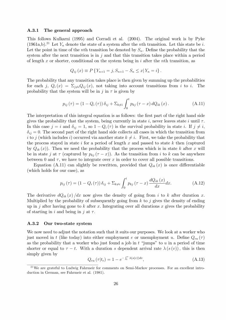
Figure 6 Illustrating transition probabilities

Let�s consider puu (�) : An individual unemployed in t can be unemployed in � by alwaysremaining unemployed. This is the term 1�Qu (�) : The individual can be unemployed in �by remaining unemployed until v where she jumps into employment, the density for whichis dQue (vjtu) =dv: After v; the probability of returning to unemployment in the remainingtime span of � � v is peu (� � v) : Note that this probability includes an arbitrary number oftransitions larger than zero in this remaining period � � v: In contrast to integrating over xas in (A.12), we integrate over the point in time v here simply as this is the more intuitiveway.As a last step, we need to determine the two derivatives dQue (v) =dv and dQeu (v) =dv.

Given duration-dependent arrival rates, the derivatives of (A.13) are,

dQue (v)

dv= e�

R vt �(s(y))dy

d

dv

Z v

t

� (s (y)) dy = e�R vt �(s(y))dy� (s (v)) (A.16a)

dQeu (v)

dv= e�

R vt �(s(y))dy

d

dv

Z v

t

� (s (y)) dy = e�R vt �(s(y))dy� (s (v)) : (A.16b)

27

Given (A.14) and the derivatives, the equations (A.15) become

puu (�) = e�R �t �(s(y))dy +

Z �

t

peu (� � v) e�R vt �(s(y))dy� (s (v)) dv;

peu (�) =

Z �

t

puu (� � v) e�R vt �(s(y))dy� (s (v)) dv:

The �nal adjustment we need to make is to replace � (s (v)) by � as the separation rate isassumed to be constant. This then gives equations (13) in the main text.

B Appendix

All references to appendices starting with B are available upon request.

References

Abbring, J., G. van den Berg, and J. van Ours (2005): �E¤ect of Unemployment InsuranceSanctions on the Transition rate from Unemployment to Employment,�Economic Journal,115, 602�630.

Acemoglu, D., and R. Shimer (1999): �E¢ cient Unemployment Insurance,�Journal of Po-litical Economy, 107, 893�928.

Albrecht, J., and S. Vroman (2005): �Equilibrium Search with Time-varying UnemploymentBene�ts,�The Economic Journal, 115, 631�648.

Arulampalam, W., and M. Stewart (1995): �The Determinants of Individual UnemploymentDuration in an Era of High Unemployment,�Economic Journal, 105, 321�332.

Blanchard, O., and P. Diamond (1994): �Ranking, Unemployment Duration, and Wages,�Review of Economic Studies, 61, 417�434.

Blanchard, O., and J. Wolfers (2000): �The Role of Shocks And Institutions In the Rise OfEuropean Unemployment: The Aggregate Evidence,�Economic Journal, 110, C1�C33.

Blos, K., and H. Rudolph (2005): �Verlierer, aber auch Gewinner,� IAB Kurzbericht, 17,1�6.

Bontemps, C., J.-M. Robin, and G. van den Berg (1999): �An Empirical Equilibrium JobSearch Model with Search on the Job and Heterogeneous Workers and Firms,� Interna-tional Economic Review, 40, 1039�1072.

Cahuc, P., and E. Lehmann (2000): �Should unemployment bene�ts decrease with the un-employment spell?,�Journal of Public Economics, 77, 135�153.

Cahuc, P., F. Postel-Vinay, and J.-M. Robin (2006): �Wage Bargaining with On-the-jobSearch: Theory and Evidence,�Econometrica, 74, 323�365.

28

Carling, K., B. Holmlund, and A. Vejsiu (2001): �Do Bene�t Cuts Boost Job Findings,�Economic Journal, 111, 766�790.

Coles, M., and A. Masters (2004): �Duration-Dependent Unemployment Insurance Paymentsand Equilibrium Unemployment,�Economica, 71, 83�97.

(2007): �Re-entitlement e¤ects with duration-dependent unemployment insurancein a stochastic matching equilibrium,� Journal of Economic Dynamics and Control, 31,2879�2898.

Coles, M. G., and A. Muthoo (2003): �Bargaining in a non-stationary environment,�Journalof Economic Theory, 109, 70�89.

Coles, M. G., and R. Wright (1998): �A Dynamic Equilibrium Model of Search, Bargaining,and Money,�Journal of Economic Literature, 78, 32�54.

Corradi, G., J. Janssen, and R. Manca (2004): �Numerical Treatment of HomogeneousSemi-Markov Processes in Transient Case - a Straightforward Approach,�Methodologyand Computing in Applied Probability, 6, 233 �246.

Diamond, P. A. (1982): �Aggregate Demand Management in Search Equilibrium,�Journalof Political Economy, 90, 881�94.

Eckstein, Z., and G. van den Berg (2007): �Empirical Labor Search: A Survey,�Journal ofEconometrics, 136, 531�564.

Fahrmeir, L., H. L. Kaufmann, and F. Ost (1981): Stochastische Prozesse. Eine Einführungin Theorie und Anwendungen. Hanser Fachbuchverlag.

Ferrall, C. (1997): �Unemployment Insurance Eligibility and the School-to-Work Transitionin Canada and the United States,�Journal of Business & Economic Statistics, 15, 115�129.

Flinn, C. (2006): �MinimumWage E¤ects on Labor Market Outcomes under Search, Match-ing, and Endogenous Contact Rates,�Econometrica, 74, 1013�1062.

Fredriksson, P., and B. Holmlund (2001): �Optimal Unemployment Insurance in SearchEquilibrium,�Journal of Labor Economics, 19, 370�399.

Hall, R. E., and P. R. Milgrom (2008): �The Limited In�uence of Unemployment on theWage Bargain,�American Economic Review, June 2008.

Heckman, J., and G. Borjas (1980): �Does Unemployment Cause Future Unemployment?De�nitions, Questions and Answers from a Continuous Time Model of Heterogeneity andState Dependence,�Economica, 47, 247�283.

Hopenhayn, H. A., and J. P. Nicolini (1997): �Optimal Unemployment Insurance,�Journalof Political Economy, 105, 412�438.

Hosios, A. J. (1990): �On the E¢ ciency of Matching Models and Related Models of Searchand Unemployment,�Review of Economic Studies, 57, 279�298.

29

Hujer, R., and H. Schneider (1989): �The Analysis of Labour Market Mobility Using PanelData,�European Economic Review, 33, 530�536.

Kulkarni, V. G. (1995): Modeling and Analysis of Stochastic Systems. Chapman & Hall.

Lancaster, T. (1990): The Econometric Analysis of Transition Data. Cambridge UniversityPress.

Ljungqvist, L., and T. J. Sargent (1998): �The European Unemployment Dilemma,�Journalof Political Economy, 106(3), 514�550.

(2007a): �Understanding European unemployment with a representative family,�Journal of Monetary Economics, 54, 2180�2204.

(2007b): �Understanding European unemployment with matching and search-islandmodels,�Journal of Monetary Economics, 54, 2139�2179.

Mo¢ tt, R., and W. Nicholson (1982): �The E¤ect of Unemployment Insurance on Unem-ployment: The Case of Federal Supplemental Bene�ts,� The Review of Economics andStatistics, 64, 1�11.

Mongrain, S., and J. Roberts (2005): �Unemployment Insurance and Experience Rating:Insurance versus E¢ ciency,�International Economic Review, 46, 1303�1319.

Mortensen, D. (1977): �Unemployment Insurance and Job Search Decisions,�Industrial andLabor Relations Review, 30, 505�517.

Mortensen, D. T. (1982): �Property Rights and E¢ ciency in Mating, Racing, and RelatedGames,�American Economic Review, 72, 968�79.

Mortensen, D. T., and C. A. Pissarides (1999): �New developments in models of search inthe labor market,�in Handbook of Labor Economics, ed. by O. Ashenfelter, and D. Card,chap. 39, pp. 2567�2627. Elsevier.

Moscarini, G. (2005): �Job Matching and the Wage Distribution,� Econometrica, 73(2),481½U516.

OECD (2004): Bene�ts and Wages. OECD, Paris.

(2007): Bene�ts and Wages. "Daten und Gra�ken", downloaded fromwww.oecd.org/de/bene�tsandwages on 12 June 2008.

Pissarides, C. A. (1985): �Short-run Equilibrium Dynamics of Unemployment Vacancies,and Real Wages,�American Economic Review, 75, 676�90.

Postel-Vinay, F., and J.-M. Robin (2002): �Equilibrium Wage Dispersion with Worker andEmployer Heterogeneity,�Econometrica, 70, 2295�2350.

Pyke, R. (1961a): �Markov Renewal Processes: De�nitions and Preliminary Properties,�The Annals of Mathematical Statistics, 32, 1231�1242.

30

(1961b): �Markov Renewal Processes with Finitely Many States,�The Annals ofMathematical Statistics, 32, 1243�1259.

Rogerson, R., R. Shimer, and R. Wright (2005): �Search-Theoretic Models of the LaborMarket: A Survey,�Journal of Economic Literature, 43, 959�988.

Ross, S. M. (1996): Stochastic processes, 2nd edition. Academic Press, San Diego.

Røed, K., and T. Zhang (2003): �Does Unemployment Compensation A¤ect UnemploymentDuration?,�Economic Journal, 113, 190�206.

Shavell, S., and L. Weiss (1979): �The Optimal Payment of Unemployment Insurance Ben-e�ts over Time,�Journal of Political Economy, 87, 1347�1362.

Shimer, R., and I. Werning (2007): �Reservation Wages and Unemployment Insurance,�Quarterly Journal of Economics, 122(3), 1145�1185.

Tanner, M., and W. H. Wong (1983): �The Estimation of the Hazard Function from Ran-domly Censored Data by the Kernel Method,�Annals of Statistics, 11, 989�993.

(1984): �Data-Based Nonparametric Estimation of the Hazard Function with Ap-plications to Model Diagnostics and Exploratory Analysis,�Journal of the American Sta-tistical Association, 79, 174�182.

van den Berg, G., B. van der Klaauw, and J. van Ours (2004): �Punitive Sanctions and theTransition from Welfare to Work,�Journal of Labor Economics, 22, 211�241.

van den Berg, G. J. (1990): �Nonstationarity in Job Search Theory,�Review of EconomicStudies, 57, 255�277.

Vuong, Q. (1989): �Likelihood Ratio Tests for Model Selection and Non-Nested Hypothesis,�Econometrica, 57, 303�333.

31

www.st-and.ac.uk/cdma

ABOUT THE CDMA

The Centre for Dynamic Macroeconomic Analysis was established by a direct grant fromthe University of St Andrews in 2003. The Centre funds PhD students and facilitates a programmeof research centred on macroeconomic theory and policy. The Centre has research interests in areassuch as: characterising the key stylised facts of the business cycle; constructing theoretical modelsthat can match these business cycles; using theoretical models to understand the normative andpositive aspects of the macroeconomic policymakers' stabilisation problem, in both open andclosed economies; understanding the conduct of monetary/macroeconomic policy in the UK andother countries; analyzing the impact of globalization and policy reform on the macroeconomy;and analyzing the impact of financial factors on the long-run growth of the UK economy, fromboth an historical and a theoretical perspective. The Centre also has interests in developingnumerical techniques for analyzing dynamic stochastic general equilibrium models. Its affiliatedmembers are Faculty members at St Andrews and elsewhere with interests in the broad area ofdynamic macroeconomics. Its international Advisory Board comprises a group of leadingmacroeconomists and, ex officio, the University's Principal.

Affiliated Members of the School

Dr Fabio Aricò.Dr Arnab Bhattacharjee.Dr Tatiana Damjanovic.Dr Vladislav Damjanovic.Prof George Evans.Dr Gonzalo Forgue-Puccio.Dr Laurence Lasselle.Dr Peter Macmillan.Prof Rod McCrorie.Prof Kaushik Mitra.Prof Charles Nolan (Director).Dr Geetha Selvaretnam.Dr Ozge Senay.Dr Gary Shea.Prof Alan Sutherland.Dr Kannika Thampanishvong.Dr Christoph Thoenissen.Dr Alex Trew.

Senior Research Fellow

Prof Andrew Hughes Hallett, Professor ofEconomics, Vanderbilt University.

Research Affiliates

Prof Keith Blackburn, Manchester University.Prof David Cobham, Heriot-Watt University.Dr Luisa Corrado, Università degli Studi di Roma.Prof Huw Dixon, Cardiff University.Dr Anthony Garratt, Birkbeck College London.Dr Sugata Ghosh, Brunel University.Dr Aditya Goenka, Essex University.Prof Campbell Leith, Glasgow University.Dr Richard Mash, New College, Oxford.Prof Patrick Minford, Cardiff Business School.

Dr Gulcin Ozkan, York University.Prof Joe Pearlman, London Metropolitan

University.Prof Neil Rankin, Warwick University.Prof Lucio Sarno, Warwick University.Prof Eric Schaling, Rand Afrikaans University.Prof Peter N. Smith, York University.Dr Frank Smets, European Central Bank.Prof Robert Sollis, Newcastle University.Prof Peter Tinsley, Birkbeck College, London.Dr Mark Weder, University of Adelaide.

Research Associates

Mr Farid Boumediene.Mr Johannes Geissler.Mr Ansgar Rannenberg.Mr Qi Sun.

Advisory Board

Prof Sumru Altug, Koç University.Prof V V Chari, Minnesota University.Prof John Driffill, Birkbeck College London.Dr Sean Holly, Director of the Department of

Applied Economics, Cambridge University.Prof Seppo Honkapohja, Cambridge University.Dr Brian Lang, Principal of St Andrews University.Prof Anton Muscatelli, Heriot-Watt University.Prof Charles Nolan, St Andrews University.Prof Peter Sinclair, Birmingham University and

Bank of England.Prof Stephen J Turnovsky, Washington University.Dr Martin Weale, CBE, Director of the National

Institute of Economic and Social Research.Prof Michael Wickens, York University.Prof Simon Wren-Lewis, Oxford University.

www.st-and.ac.uk/cdma

THE CDMA CONFERENCE 2008, held in St. Andrews, 3th to the 5th of September2008.

PAPERS PRESENTED AT THE CONFERENCE, IN ORDER OF PRESENTATION:

Title Author(s) (presenter(s) in bold)

Robust Learning Stability with OperationalMonetary Policy Rules

George Evans (Oregon and St Andrews) co-authored with Seppo Honkapohja

Who pays for job training? Parantap Basu (Durham)

Electoral Uncertainty and the Deficit Bias in aNew Keynesian Economy

Campbell Leith (Glasgow)

Sacrifice Ratio or Welfare Gain Ratio?Disinflation in a DGSE monetary model

Guido Ascari (Pavia)

Estimating insurance and incentive effects oflabour market reforms

Klaus Waelde (Glasgow)

Using time-varying VARs to diagnose the sourceof 'Great Moderations': a Monte Carlo analysis

Tony Yates (Bank of England)

The Optimum Quantity of Money with GoldReserves

Max Gillman (Cardiff)

Managing Disinflation Under Uncertainty Eric Schaling (Pretoria)

Factor demand linkages and the business cycle:interpreting aggregate fluctuations as sectoralfluctuations

Sean Holly (Cambridge)

Monetary and Fiscal Rules in an EmergingSmall Open Economy

Paul Levine (Surrey) with joint with NicolettaBatini (IMF and Surrey) Joe Pearlman (LondonMet)

Can a pure Real Business Cycle Model explainthe real exchange rate?

Patrick Minford (Cardiff)

Macroeconomic Implications of a Key Currency Matthew Canzoneri (Georgetown)

How we can model the credit crunch Peter Sinclair (Birmingham)Sticky information versus efficient indexation Richard Mash (New College, Oxford

See also the CDMA Working Paper series at www.st-andrews.ac.uk/cdma/papers.html.