1

CCVT Failures and Their Effects on Distance Relays Sophie Gray, CenterPoint Energy

Derrick Haas and Ryan McDaniel, Schweitzer Engineering Laboratories, Inc. 2350 NE Hopkins Court, Pullman, WA 99163 USA, +1.509.332.1890

Abstract—Distance relays rely on accurate voltage and current signals to correctly determine if a fault is within their zone of protection, as determined by the impedance reach setting. The current signal provided to the relay comes from a current transformer (CT), which is a simple device consisting of a steel core and wire wrapped around that core. At high voltage levels, the voltage signal typically comes from a coupling-capacitor voltage transformer (CCVT), which is more complicated and less reliable than a CT. Although a CCVT is more complex than a CT, very little additional attention is typically given to monitor the performance of a CCVT. Typically, loss-of-potential (LOP) logic is used to detect a loss of the voltage signal to the relay, but the LOP logic does not effectively monitor and alarm for transient CCVT errors, errors small in scale, or errors that develop gradually.

In this paper, we review three unique CCVT failure events and discuss relay performance during these failures. We analyze the performance of two different distance relays during a CCVT failure in which the voltage applied to the relays was erratic and influenced the frequency tracking in one relay but not the other. Next, we discuss an event in which a CCVT transient led to a relay overreach but also revealed that the CCVT was failing. Last, we analyze an event in which a CCVT failure caused a standing measurement error prior to a phase-to-ground fault and evaluate the influence of a standing unbalance of the directional elements of the relay.

From these events, we offer solutions for monitoring CCVT performance that include steady-state monitoring as well as transient characteristics to look for while analyzing events.

I. INTRODUCTION Coupling-capacitor voltage transformers (CCVTs) are

generally used at transmission-level voltages (138 kV and up) to provide secondary voltage signals to relays. This is because they are more cost-effective than wire-wound potential devices rated for full system voltage. The idea behind a CCVT is to use a capacitive voltage divider to step down the voltage before feeding it into a wire-wound VT that is rated much lower than the full system voltage. While a CCVT is more economical than a wire-wound VT, it is a complex device consisting of a tapped stacked of capacitors, a tuning reactor, a wire-wound VT, a gap protection circuit, and a ferroresonance suppression circuit (active or passive). Fig. 1 shows the basic structure of a CCVT [1].

As CCVTs age, failures are more likely to occur as thermal cycling causes material degradation, applied overvoltages reduce the dielectric strength, and spark gaps become corroded. These failures can result in a slight error in the replicated secondary voltage, a corrupted voltage signal, a total loss of the voltage signal, or unexpected transient performance. Most relays have logic to monitor for a total loss of voltage (loss-of-

potential [LOP] logic), but this logic cannot necessarily detect a corrupted voltage signal, a slight error in the signal, or abnormal transient performance.

Fig. 1. Generic CCVT model

In this paper, we analyze three events in which CCVTs misbehaved in the following ways:

• Event 1: A CCVT produces a transient in which a high-speed distance element using a half-cycle filter window overreaches but a traditional full-cycle filter window distance element does not.

• Event 2: A CCVT produces a corrupted signal for which one relay was able to restrain from operation but another relay was not.

• Event 3: A CCVT produces a slight signal error that leads to an incorrect directional decision.

These three events show that traditional LOP logic is not designed to catch all CCVT failure modes. We offer ideas and solutions to detect CCVT failure modes that do not lead to a total loss of voltage.

II. CCVT TRANSIENT ANALYSIS There is a great deal of literature regarding CCVT transient

performance for traditional full-cycle filtered distance elements [2] [3] [4]. It is well-known that CCVTs tend to overshoot a voltage drop as seen by a full-cycle filtered distance element. This leads to the so-called CCVT transient overreach phenomenon in which a Zone 1 element set to underreach the remote terminal temporarily sees an external fault within the reach of Zone 1. This overreach is mitigated by adding a short delay in the operation of the Zone 1 distance element to allow time for the CCVT transient to subside. Typically, this delay is added if a source-to-impedance ratio (SIR) of five or greater is detected and the mho element calculation is not “smooth.”

The worst case of CCVT transient overreach occurs at a voltage zero crossing because this is the moment in which the capacitor has the highest amount of stored energy. Fig. 2 shows a CCVT transient from an active ferroresonance suppression circuit compared with the ideal response.

2

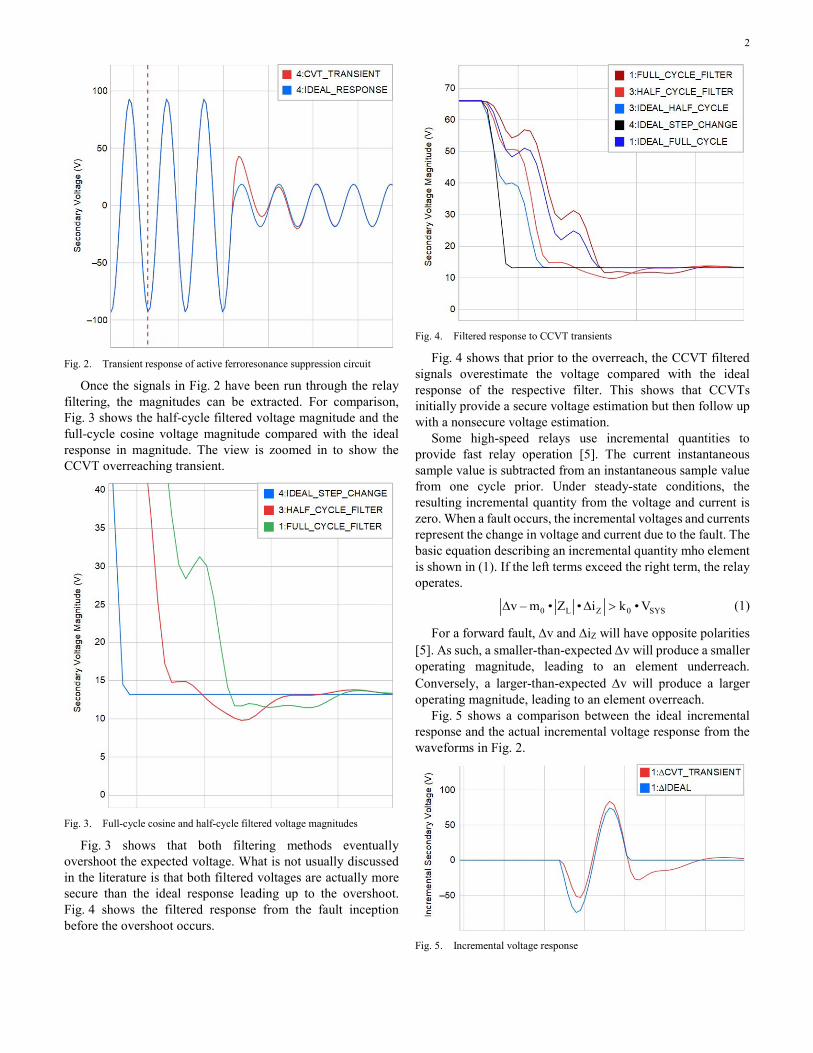
Fig. 2. Transient response of active ferroresonance suppression circuit

Once the signals in Fig. 2 have been run through the relay filtering, the magnitudes can be extracted. For comparison, Fig. 3 shows the half-cycle filtered voltage magnitude and the full-cycle cosine voltage magnitude compared with the ideal response in magnitude. The view is zoomed in to show the CCVT overreaching transient.

Fig. 3. Full-cycle cosine and half-cycle filtered voltage magnitudes

Fig. 3 shows that both filtering methods eventually overshoot the expected voltage. What is not usually discussed in the literature is that both filtered voltages are actually more secure than the ideal response leading up to the overshoot. Fig. 4 shows the filtered response from the fault inception before the overshoot occurs.

Fig. 4. Filtered response to CCVT transients

Fig. 4 shows that prior to the overreach, the CCVT filtered signals overestimate the voltage compared with the ideal response of the respective filter. This shows that CCVTs initially provide a secure voltage estimation but then follow up with a nonsecure voltage estimation.

Some high-speed relays use incremental quantities to provide fast relay operation [5]. The current instantaneous sample value is subtracted from an instantaneous sample value from one cycle prior. Under steady-state conditions, the resulting incremental quantity from the voltage and current is zero. When a fault occurs, the incremental voltages and currents represent the change in voltage and current due to the fault. The basic equation describing an incremental quantity mho element is shown in (1). If the left terms exceed the right term, the relay operates.

0 L Z 0 SYSv – m • Z • i k • V∆ ∆ > (1)

For a forward fault, ∆v and ∆iZ will have opposite polarities [5]. As such, a smaller-than-expected ∆v will produce a smaller operating magnitude, leading to an element underreach. Conversely, a larger-than-expected ∆v will produce a larger operating magnitude, leading to an element overreach.

Fig. 5 shows a comparison between the ideal incremental response and the actual incremental voltage response from the waveforms in Fig. 2.

Fig. 5. Incremental voltage response

3

The CCVT response initially produces a smaller-than-expected ∆v and the element underreaches for about the first half-cycle of the event. For the second half-cycle, ∆v is slightly larger than expected and can produce a small relay overreach. As long as the high-speed relay is shut down prior to the introduction of the overreach, it is inherently secure.

A distance relay relies on accurate voltage and current signals to determine if the fault is within its zone of protection. When are these signals the most accurate during the fault?

Interestingly, CTs and CCVTs provide the most accurate data to the relay at different times during a fault. CTs provide the most accurate fault data near fault initiation, before the effects of CT saturation set in. CCVTs, on the other hand, provide the most accurate fault data well after the fault initiation, after the effects of the CCVT transients have subsided. However, the initial data provided by a CCVT are biased toward security.

Assuming the CTs do not go into saturation for a fault, making a tripping decision within the first half-cycle of the event is inherently secure as long as the CCVT is performing as expected. Making a tripping decision after a CCVT transient has passed is more dependable because the voltage is accurately replicated.

III. EVENT ANALYSIS In this section, we look at the three events outlined in the

introduction.

A. Fast CCVT Transient Leads to High-Speed Distance Element Overreach

In this event, a poorly performing CCVT produced a transient for which the high-speed elements drastically overreached the traditional full-cycle filtered elements.

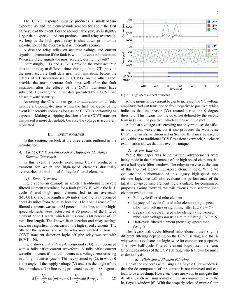
1) Event Overview Fig. 6 shows an example in which a traditional full-cycle

filtered element restrained for a fault (MCG1F) while the half-cycle filtered high-speed element led to an overreach (MCG1H). The line length is 36 miles, and the fault occurred about 45 miles from the relay location. The Zone 1 reach of the filtered elements was set at 85 percent of the line, and the high-speed elements were factory-set at 80 percent of the filtered element Zone 1 reach, which in this case is 68 percent of the total line length. The known fault location and relay settings indicate a significant overreach of the high-speed elements. The SIR for the system is 2, so the relay user elected to turn the CCVT transient detection logic off (the relay was set with ECVT = N).

Fig. 6 shows that a Phase-C-to-ground (CG) fault occurred with a fully offset current waveform. A fully offset current waveform occurs if the fault occurs at a voltage zero crossing in a fully inductive system. This is explained by (2), in which θ is the angle of the supply voltage (V) and ϕ is the angle of the line impedance. The line being protected has a ϕ of 88 degrees.

( ) ( ) ( )R– tm m LV V

i t sin t – – sin – eZ Z

= ω + θ ϕ θ ϕ (2)

Fig. 6. High-speed element overreach

At the moment the current began to increase, the VC voltage amplitude had just transitioned from negative to positive, which indicates that the phasor (Vc) rotated across the 0 degree threshold. This means that the dc offset defined by the second term in (2) will be positive, which agrees with the plot.

A fault at a voltage zero crossing not only produces dc offset in the current waveform, but it also produces the worst-case CCVT transients, as discussed in Section II. It may be easy to chalk this up to traditional CCVT transient overreach, but closer examination shows that this event is unique.

2) Event Analysis While this paper was being written, advancements were

being made in the performance of the high-speed elements that use a half-cycle filter window. The relay in service at the time of this trip had legacy high-speed element logic. While we evaluate the performance of this legacy high-speed mho element logic, we will also evaluate the performance of the latest high-speed mho element logic available for comparison purposes. Going forward, we will discuss four separate mho element evaluations:

• Full-cycle filtered mho element • Legacy half-cycle filtered mho element (high-speed

mho) with voltages using mimic filter (ECVT = Y) • Legacy half-cycle filtered mho element (high-speed

mho) with voltages not using mimic filter (ECVT = N) • Half-cycle filtered element (new high-speed mho

design) The legacy half-cycle filtered mho element uses slightly

different filtering depending on the ECVT setting, and that is why we must evaluate that logic twice for comparison purposes. The new half-cycle filtered element logic uses the same filtering regardless of the ECVT setting, which allows for much easier analysis.

a) High-Speed Element Filtering One of the concerns with using a half-cycle filter window is

that the dc component of the current is not removed and can lead to overreaching. However, there are ways to mitigate this dc offset, such as using a mimic filter in conjunction with the half-cycle window [6]. With the properly selected mimic filter,

4

the dc offset from a half-cycle cosine filter can be nearly eliminated [6].

Fig. 7 compares the full-cycle filtered and the half-cycle filtered IC current magnitudes to illustrate that there is no current overshoot in either signal, which is quite impressive given the known dc offset in the original signal. As a reference, the two vertical cursors show the time during which the high-speed element was asserted in the relay.

Fig. 7. IC magnitude (full-cycle filtered and half-cycle filtered)

Next, we look at the voltage magnitudes of the full-cycle and half-cycle filtered voltages. This brings up the question, Is the mimic filter used in the voltage signal as well? In the legacy half-cycle filtered elements, the use of the mimic filter depends on whether the CCVT transient detection logic is turned on in the relay. If ECVT = Y, then the voltages are run through a mimic filter the same as the currents. If ECVT = N, the voltages are not run through a mimic filter and their phase angles are adjusted such that the mimic filter delay introduced to the current signal is compensated for in the voltage phasors. With ECVT = N, the relay provides a slightly faster trip time than if ECVT = Y. However, ECVT = Y provides a bit more filtering to help smooth out the voltage signal.

This method works well enough, but there can still be significant transient overshoot caused by the CCVT transients providing an unstable signal. Because of this, the legacy half-cycle mho element reaches are pulled back from the full-cycle element reach. If ECVT = N, the legacy high-speed element reach is set at 80 percent of the full-cycle element reach. If ECVT = Y, then the legacy high-speed element reach is set at 70 percent of the full-cycle element reach. The side effect is that, if a fault occurs near the reach point set in the relay, there is little hope of tripping on the high-speed element. Effectively, the legacy high-speed element is useful for faults within 60 to 68 percent of the total line length rather than 85 percent of the total line length Zone 1 setting.

To further dampen the CCVT transients with a negligible sacrifice to speed, a low-pass filter is used in conjunction with the mimic filter in the new half-cycle filtered element. The result is that the new high-speed mho elements have greatly mitigated transient overshoot so that they can have the same reach as the full-cycle elements.

Fig. 8 shows the plot of the full-cycle filtered, the legacy half-cycle filtered (with no mimic filter), and the new half-cycle filtered VC magnitudes. Again, the two cursors show the time during which the high-speed element asserted.

Fig. 8. Comparison of various VC filtered values

Fig. 8 shows that the legacy half-cycle filtered element with no mimic filter, which is used when ECVT = N, had the most overshoot. This was the voltage signal used by the mho element at the time of the trip.

b) Mho Element Evaluation In Fig. 9, we evaluate the CG mho element four times using

the four different filtering methods discussed previously. Recall that the mimic filter is always used on the current signal, but in the legacy implementation, the mimic filter in used on the voltage signal only if ECVT = Y. In the new high-speed element, the mimic and low-pass filters are used on both the voltage and current signals.

Fig. 9. CG mho element evaluations

The bottom section of Fig. 9 shows that the full-cycle filtered mho element restrained for this fault. In fact, at the time of the trip (marked by the orange cursor) the calculated CG impedance of the full-cycle filtered element was 4.14 ohms, which is four times larger than the set reach of 1.02. The lowest impedance seen by the full-cycle filtered mho element was 1.33 ohms, which is about 30 percent beyond the Zone 1 reach.

Time-delaying the Zone 1 element to provide security was not required because it did not see a CCVT transient producing an overreach in the full-cycle filtered mho calculation. From a full-cycle filtered element standpoint, setting ECVT = Y would not have provided any benefit.

5

Clearly, the overreach issue is with the high-speed elements. Referring to Fig. 9, we note the following regarding the high-speed mho elements:

• The legacy high-speed mho element with no voltage mimic filter (ECVT = N) overreaches even with the conservative reach of 68 percent of the line length.

• The legacy high-speed mho element (ECVT = Y) does not overreach the conservative reach of 60 percent of the line length. The relay would have restrained if ECVT = Y with the legacy high-speed mho elements. The legacy filtering still allows an overreach if the element reach is set at 85 percent of the line length.

• The improved high-speed mho (ECVT = Y or N) does not overreach with a reach of 85 percent of the line length and would have been secure for this event.

Although the ECVT setting has no effect on the new high-speed mho element filtering, it does affect the security counts used by the relay. In general, ECVT = N provides slightly faster tripping than ECVT = Y. This is also true of the legacy high-speed element design. This difference in relay operation speed affects the high-speed elements regardless of whether there has been an actual CCVT transient detected.

c) Further Analysis After the evaluation of the high-speed mho elements, it may

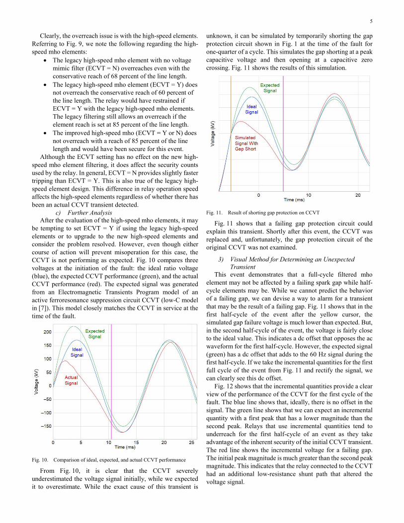
be tempting to set ECVT = Y if using the legacy high-speed elements or to upgrade to the new high-speed elements and consider the problem resolved. However, even though either course of action will prevent misoperation for this case, the CCVT is not performing as expected. Fig. 10 compares three voltages at the initiation of the fault: the ideal ratio voltage (blue), the expected CCVT performance (green), and the actual CCVT performance (red). The expected signal was generated from an Electromagnetic Transients Program model of an active ferroresonance suppression circuit CCVT (low-C model in [7]). This model closely matches the CCVT in service at the time of the fault.

Fig. 10. Comparison of ideal, expected, and actual CCVT performance

From Fig. 10, it is clear that the CCVT severely underestimated the voltage signal initially, while we expected it to overestimate. While the exact cause of this transient is

unknown, it can be simulated by temporarily shorting the gap protection circuit shown in Fig. 1 at the time of the fault for one-quarter of a cycle. This simulates the gap shorting at a peak capacitive voltage and then opening at a capacitive zero crossing. Fig. 11 shows the results of this simulation.

Fig. 11. Result of shorting gap protection on CCVT

Fig. 11 shows that a failing gap protection circuit could explain this transient. Shortly after this event, the CCVT was replaced and, unfortunately, the gap protection circuit of the original CCVT was not examined.

3) Visual Method for Determining an Unexpected Transient

This event demonstrates that a full-cycle filtered mho element may not be affected by a failing spark gap while half-cycle elements may be. While we cannot predict the behavior of a failing gap, we can devise a way to alarm for a transient that may be the result of a failing gap. Fig. 11 shows that in the first half-cycle of the event after the yellow cursor, the simulated gap failure voltage is much lower than expected. But, in the second half-cycle of the event, the voltage is fairly close to the ideal value. This indicates a dc offset that opposes the ac waveform for the first half-cycle. However, the expected signal (green) has a dc offset that adds to the 60 Hz signal during the first half-cycle. If we take the incremental quantities for the first full cycle of the event from Fig. 11 and rectify the signal, we can clearly see this dc offset.

Fig. 12 shows that the incremental quantities provide a clear view of the performance of the CCVT for the first cycle of the fault. The blue line shows that, ideally, there is no offset in the signal. The green line shows that we can expect an incremental quantity with a first peak that has a lower magnitude than the second peak. Relays that use incremental quantities tend to underreach for the first half-cycle of an event as they take advantage of the inherent security of the initial CCVT transient. The red line shows the incremental voltage for a failing gap. The initial peak magnitude is much greater than the second peak magnitude. This indicates that the relay connected to the CCVT had an additional low-resistance shunt path that altered the voltage signal.

6

Fig. 12. Incremental quantities of expected signal (green), ideal signal (blue), and gap short signal (red)

These signals are easy to acquire using event analysis software. In time-domain relays, the incremental signals are available directly from the relay, allowing for easy visual inspection of the CCVT transient performance. Tracking these signals for events over time can alert a user to a poorly performing CCVT.

B. Corrupted Voltage Signal Leads to Zone 1 Trip in One Relay, but Not in Another

This event demonstrates the effects a failing CCVT can have on LOP logic.

1) Event Overview Two relays protect a 765 kV line in which the Phase A

voltage becomes erratic during load conditions. Relay A correctly declares an LOP condition, and this condition stays sealed in. Relay B also initially declares an LOP condition, but then the LOP signal drops out. Fig. 13 shows the filtered load current for the protected circuit on the top axis, the filtered phase voltages from the CCVT on the middle axis, the unfiltered Phase A voltage from the CCVT on the bottom axis, and the LOP declarations of Relay A and Relay B. Relay A and Relay B use the same CCVT for voltages and saw the same currents during this event. However, only a filtered event was retrieved from Relay A, while an unfiltered event was retrieved from Relay B.

The unfiltered voltage in Fig. 13 shows that the voltage signal from the CCVT became corrupted. Harmonic analysis performed on the signal shows that the total harmonic distortion went from 0 percent prior to the relay LOP assertion to 40 percent after the LOP assertion. While the unfiltered signal shows that there is an issue with the Phase A voltage, the filtered signal (which contains only the 60 Hz content) shows a less dramatic change. The filtered VA signal reduced in magnitude from 445 kV to about 290 kV, and a 20 degree phase shift was introduced.

Fig. 13. Initial failure of CCVT on Phase A voltage

Fig. 13 shows that the Relay B protection elements that rely on voltage are vulnerable due to the deassertion of the LOP logic. In fact, nearly two seconds after the LOP deassertion in Relay B, the Zone 1 distance elements asserted, issuing a trip to the circuit breaker and isolating the line (Fig. 14). By this time, the filtered VA magnitude had declined to about 160 kV.

Fig. 14. Relay B issuing trip after LOP deassertion

While Relay A and Relay B have different hardware platforms, both relays use nearly identical logic to detect an LOP condition. Why does one relay seal in the LOP condition while the other relay does not?

2) LOP Overview The LOP logic in Relay A and Relay B uses phasor

incremental quantities over the course of one cycle to detect an LOP condition. The LOP logic is primarily designed to catch blown fuse conditions on a VT at the moment the fuse blows and to block relay elements that can misoperate for this loss of voltage. If a fuse is blown on a potential device, the relay will

7

see a sharp drop in voltage. However, since the system is unaffected by this blown fuse, the current seen by the relay will remained unchanged. A system fault can also lead to a sharp drop in the voltage seen by the relay, but that event is also accompanied by a change in current. So, a very basic relationship is used in incremental quantity LOP detection: if there is a current change, block the LOP bit from asserting; otherwise, allow the LOP bit to assert for a decay in voltage [8].

Three conditions must be met for an LOP bit to assert: • A 10 percent or greater decrease in positive-sequence

voltage magnitude (V1) from the phasor one cycle prior.

• No appreciable change in the positive-sequence current (I1) from the phasor one cycle prior.

• No appreciable change in the zero-sequence current phasor (I0) from the phasor one cycle prior.

“Appreciable current change” is defined as a secondary current magnitude change of more than 0.02 • 5 A nominal (0.1 A secondary) or a current angle change of more than 5 degrees over the last cycle.

The following equations express the three LOP conditions in more specific terms, where k is defined as the present phasor value and k–1 cycle is defined as the phasor value from one cycle ago.

k k –1 cycleV1 0.9 • V1≤ (3)

k k –1 cycle k k –1 cycleI1 – I1 0.1 or I1 – I1 5> ∠ ∠ > (4)

k k –1 cycle k k –1 cycleI0 – I0 0.1 or I0 – I0 5> ∠ ∠ > (5)

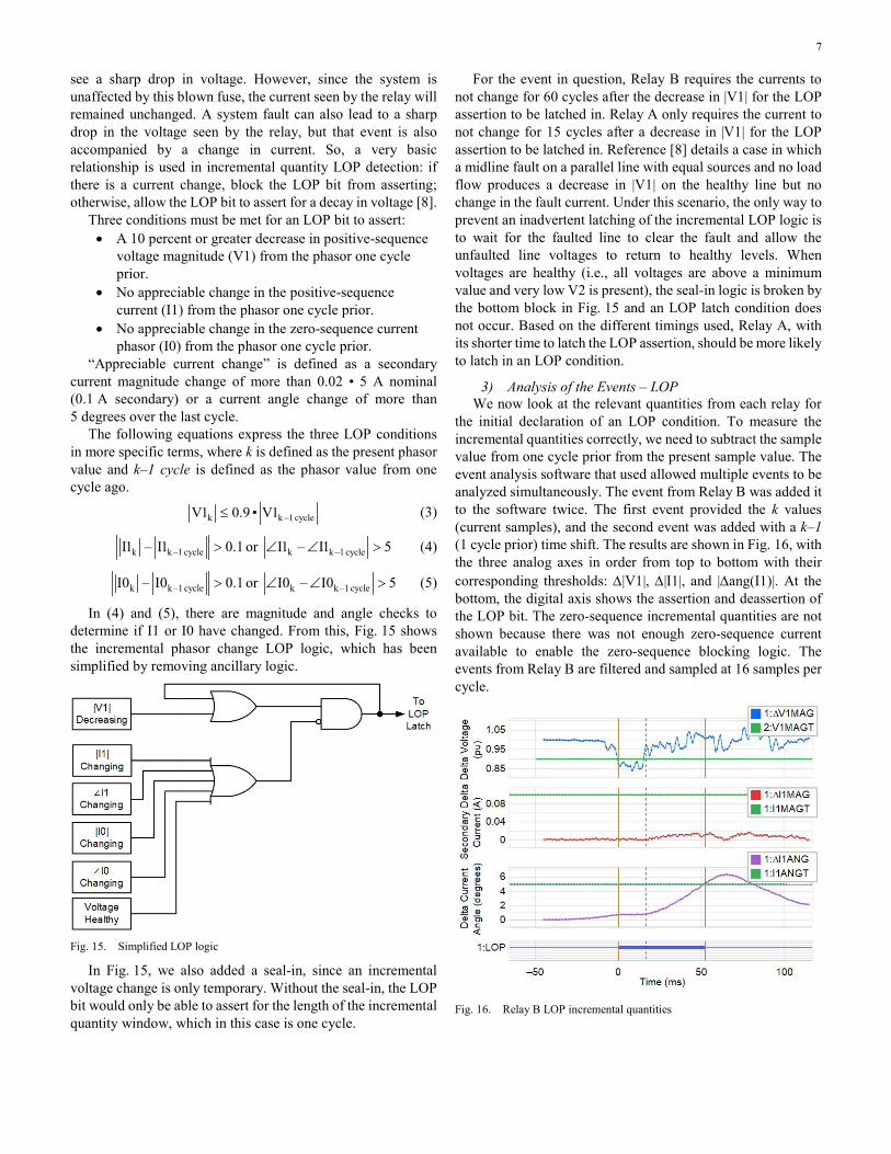
In (4) and (5), there are magnitude and angle checks to determine if I1 or I0 have changed. From this, Fig. 15 shows the incremental phasor change LOP logic, which has been simplified by removing ancillary logic.

Fig. 15. Simplified LOP logic

In Fig. 15, we also added a seal-in, since an incremental voltage change is only temporary. Without the seal-in, the LOP bit would only be able to assert for the length of the incremental quantity window, which in this case is one cycle.

For the event in question, Relay B requires the currents to not change for 60 cycles after the decrease in |V1| for the LOP assertion to be latched in. Relay A only requires the current to not change for 15 cycles after a decrease in |V1| for the LOP assertion to be latched in. Reference [8] details a case in which a midline fault on a parallel line with equal sources and no load flow produces a decrease in |V1| on the healthy line but no change in the fault current. Under this scenario, the only way to prevent an inadvertent latching of the incremental LOP logic is to wait for the faulted line to clear the fault and allow the unfaulted line voltages to return to healthy levels. When voltages are healthy (i.e., all voltages are above a minimum value and very low V2 is present), the seal-in logic is broken by the bottom block in Fig. 15 and an LOP latch condition does not occur. Based on the different timings used, Relay A, with its shorter time to latch the LOP assertion, should be more likely to latch in an LOP condition.

3) Analysis of the Events – LOP We now look at the relevant quantities from each relay for

the initial declaration of an LOP condition. To measure the incremental quantities correctly, we need to subtract the sample value from one cycle prior from the present sample value. The event analysis software that used allowed multiple events to be analyzed simultaneously. The event from Relay B was added it to the software twice. The first event provided the k values (current samples), and the second event was added with a k–1 (1 cycle prior) time shift. The results are shown in Fig. 16, with the three analog axes in order from top to bottom with their corresponding thresholds: ∆|V1|, ∆|I1|, and |∆ang(I1)|. At the bottom, the digital axis shows the assertion and deassertion of the LOP bit. The zero-sequence incremental quantities are not shown because there was not enough zero-sequence current available to enable the zero-sequence blocking logic. The events from Relay B are filtered and sampled at 16 samples per cycle.

Fig. 16. Relay B LOP incremental quantities

8

Fig. 16 shows that the ratio of |V1k| / |V1k–1 cycle| (DV1) did go lower than 0.9 (V1T), indicating that there was enough change in V1 to allow an LOP assertion. However, it did not exceed this threshold by much. The lowest recorded DV1 was 0.85, which means there was a 15 percent change in V1. This is only 1.5 times the necessary 10 percent change.

Fig. 16 also shows that while the magnitude of I1 (DI1MAG) did not appear to change, the angle of I1 (DI1ANG) did change slowly, from nearly zero at the time of the LOP declaration to 5 at the time the LOP bit dropped out. It took about three cycles for DI1ANG to go from 0 to 5 degrees. When the DI1ANG value exceeded 5 degrees, the LOP bit deasserted because a large enough change in current was detected.

The pertinent incremental quantities for Relay A, which was looking at the same voltage and current signals, are shown in Fig. 17. The events from Relay A are filtered and sampled at 4 samples per cycle.

Fig. 17. Relay A LOP incremental quantities

Aside from the higher resolution available from the event reports in Relay B, the Relay A DV1 signal looks similar to that of Relay B. However, DI1ANG did not change in Relay A, which prevented the LOP bit from being blocked in Relay A. This analysis of incremental quantities shows that Relay B saw a change in the I1 angle while Relay A did not. The question is, why?

Based on a closer inspection of the IΦ k and IΦk–1 cycle signals (where Φ = A, B, or C) from Relay B, it appears that all of the current signals were sampled at a slightly different part of the sine wave shortly after the LOP condition was detected. Fig. 18 shows only the IAk (blue) and IAk–1 cycle (purple) currents for simplicity.

We expect that even if these two signals are one cycle apart in time, they would still look exactly the same and be sampled the same. This is true for the left side of the plot, before the LOP condition occurred.

Shortly after the LOP condition was declared by the relay, the IAk samples appear to occur before the IAk–1 cycle samples on the sine wave. This means that the time difference between IAk

and IAk–1 cycle is actually less than one cycle. Since the time differential between the two signals is not equal to one cycle,

the quantity DI1ANG is no longer equal to zero. In this case, the signed value of DI1ANG evaluates to about –6 degrees at the peak of the calculation, indicating that |I1k| is lagging |I1k–1 cycle|.

Fig. 18. Relay B IAk and IAk–1 cycle signals

In Relay B, the sampling rate of all the signals is determined by the frequency tracking algorithm, which relies on the VA signal. The relay looks at the time between the zero crossings of the signal to determine the frequency [9]. For a 60 Hz signal, zero crossings should occur every 8.33 milliseconds. Fig. 19 compares the expected voltage and the actual voltage from Relay B. The actual voltage made a zero crossing well before the next zero crossing was expected to occur, which indicates an abrupt change in frequency.

Fig. 19. Relay B unfiltered VA voltage and expected VA voltage

Using the zero-crossing times, we can calculate the period of the signal and from that the frequency.

The four zero crossings that occurred after the LOP assertion were evaluated at the following frequencies: 65 Hz, 62.4 Hz, 58.58 Hz, and 60 Hz. Relay B rejects frequencies in excess of 65 Hz, so none of the frequency measurements were rejected. Relay B detected this sudden increase in the apparent frequency and slowly increased the sampling rate. The sampling rate does not change instantaneously; it is slowly sped up or slowed down to prevent abrupt signal changes. However, even a slow change in the sampling rate leads to a phase angle difference in the incremental quantities. For example, sampling a 60 Hz signal

9

at 61 Hz leads to a 6 degree angular slip over the time period of the 60 Hz signal (16.6 milliseconds). This 6 degree difference between the incremental quantities continues until the sampling rate of the relay agrees with the frequency of the signal the relay is trying to sample. Fig. 16 shows that toward the end of the event, DI1ANG is reducing. This indicates that the sample rate of the relay is correct for the signal provided. The VA voltage, after the initial failure, does tend to have zero crossings closer to the expected 8.33 milliseconds for a 60 Hz signal.

Relay B had a new firmware revision that caused it to ignore large changes in frequency, thus preventing these changes from influencing the sample rate of the relay. This may have prevented the LOP bit from deasserting in this case. It is a good practice to keep relay firmware up to date.

The Relay A frequency tracking is vastly improved over the legacy algorithm in Relay B. Relay A does not rely on VA alone to track the voltage, using instead the Alpha Voltage, which is a mathematical combination of VA, VB, and VC [10]. Therefore, VA is not the only influence on zero-crossing detection. In addition, Relay A rejects the highest and lowest frequencies from the last four cycles and averages the remaining two. This “truncated mean” allows the relay to remove outliers from the frequency tracking, which in this case removed the short-lived frequency excursions. In addition, Relay A had logic to detect and reject large step changes in frequency.

In conclusion, the superior frequency tracking algorithm in Relay A allowed the LOP bit to latch in and block relay elements that rely on voltage. This prevented Relay A from operating during this loss of voltage. However, we still want to know why Relay B did operate for this condition, since failing to latch the LOP bit was not the only thing that led to the eventual operation of Relay B.

4) Analysis of Events – Distance Elements Fig. 14 shows that the word bit M1P asserts in Relay B,

which is a phase mho element. This is surprising because the voltage was lost on a single phase, not on two or more phases. However, the relay uses fault identification logic based on currents to determine which mho elements to release for operation [11]. In this case, because the currents are balanced (load conditions), the AB, BC, and CA mho elements are available to operate. In fact, all three phase loops operated at the same time in Relay B. The ground elements are blocked when no zero-sequence current is present.

It is common to calculate the apparent impedance seen by the relay by dividing the faulted phase voltage by the faulted phase current. In this case, we select the ZAB impedance, which is equal to VAB / IAB. This evaluates to 15 ohms secondary at the time of the M1P assertion. The Zone 1 element was set at 3.3 ohms secondary. This is not a small enough apparent impedance to get the Zone 1 element to operate, so why did the element operate?

Modern day mho elements use memory voltage as a polarizing quantity, which relies on accurate frequency tracking for element security. Equation (6) shows the AB mho element formula.

( )( )

( )( )( )*

*

Re VAB VAB1memMAB

Re 1 Z1L IAB VAB1mem=

∠ (6)

Under load and most fault conditions, the phasor VAB and the phasor VAB1mem are in phase with each other. However, if the frequency tracking of the relay is incorrect, then the two phasors slip from each other as time progresses. This situation is more drastic than the angular displacement experienced with an incremental quantity. In incremental quantities, the memory of the signal is only one sample from one cycle prior, and it is weighted equally to the present sample. A slip in the sampling frequency can directly be related to the phase angle error in this case. Memory voltage, however, heavily weights previous information over present information using an infinite input response. Because past information is weighted so heavily, it takes time for the memory signal to adapt to changes in the sampling frequency. Because of this, the slip between a signal and its memory produces a cumulative slip over time before stabilization is reached. Fig. 20 shows the angular displacement between a signal (V) and its memory (Vmem) as time progresses.

Fig. 20. ang(V1mem) – ang(V)

V is a 60 Hz signal that is sampled at 61 Hz with 16 samples per sample period. Vmem is defined in (7).

k k k –161 15Vmem • V Vmem

16 16= + (7)

The angle of V is calculated using (8). Vmem is calculated similarly.

( ) –1 k –4k

k

Vang V tan

V= (8)

In this case, the angular displacement stabilizes at about 55 degrees after the frequency tracking error is introduced. This demonstrates that correct frequency tracking is crucial in elements that use weighted signal memory. The situation can become even worse if the frequency tracking is changing erratically due to a failing voltage potential, which is likely in this particular event.

Returning our attention to (6), we see that the numerator gets its sign based on the cosine of the angular difference between phasor VAB and phasor VABmem. If the angular difference between these two quantities is greater than 90 degrees, the numerator evaluates to a negative number.

10

The denominator of the mho element serves as a directional element to supervise the mho. If the sign of the denominator is positive, the mho element is allowed to operate. If the numerator is negative and the denominator is positive, MAB will be negative, ensuring a mho element operation since a negative number will be less than a positive set point. This is how Relay B was able to trip for this event, even though the apparent impedance was above the set point.

The event report from Relay B provides the following phase angles for the pertinent quantiles needed in (6) at the time of M1P assertion:

• ang(VAB) = 0° • ang(VAB1mem) = 140° • ang(Ζ1L) = 88° • ang(ΙΑΒ) = −25.2°

Evaluating the numerator results in the following: cos(∠0 − ∠140°) = negative

Evaluating the denominator results in the following: cos(∠88° + ∠–25.2° – ∠140°) = positive

From this evaluation, the conditions are met for the mho element to operate. The memory voltage became corrupted from the failing CCVT on Phase A, and the mho element was able to operate.

C. Standing CCVT Error Causes Incorrect Direction Element Decision

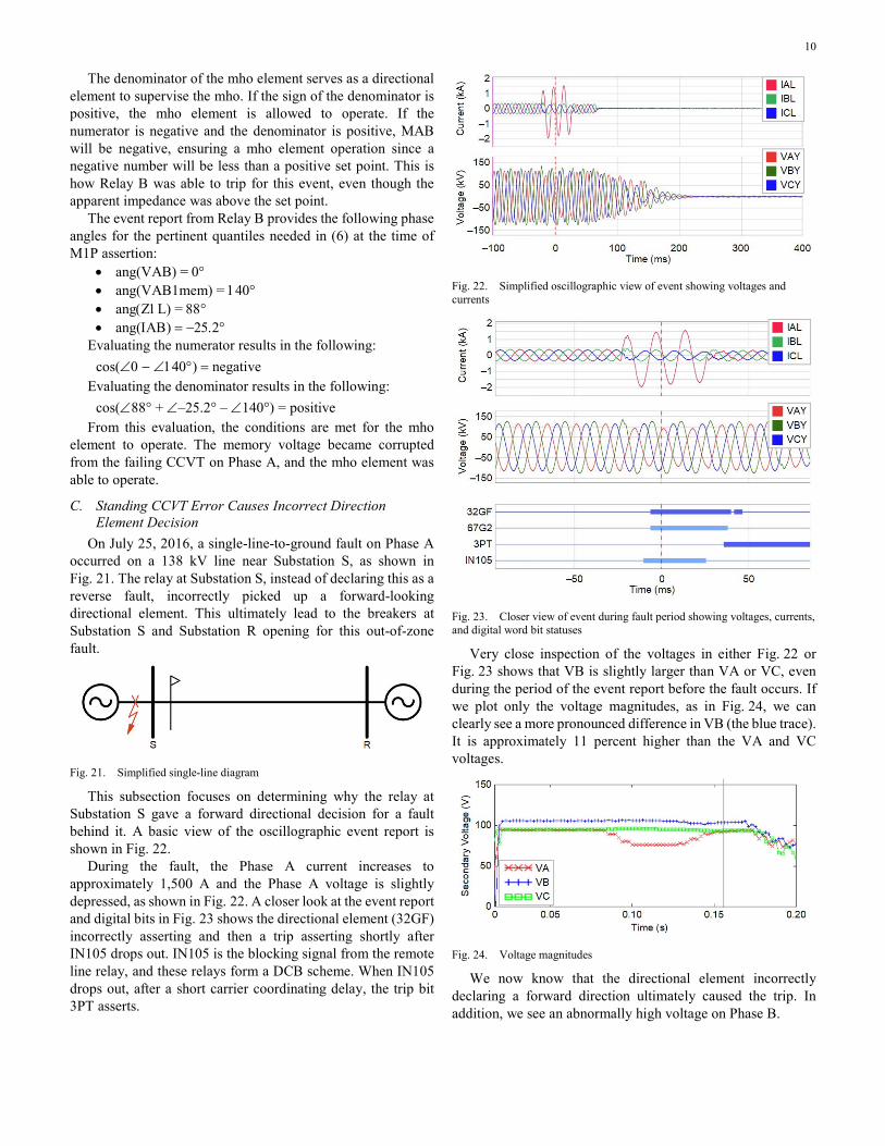
On July 25, 2016, a single-line-to-ground fault on Phase A occurred on a 138 kV line near Substation S, as shown in Fig. 21. The relay at Substation S, instead of declaring this as a reverse fault, incorrectly picked up a forward-looking directional element. This ultimately lead to the breakers at Substation S and Substation R opening for this out-of-zone fault.

Fig. 21. Simplified single-line diagram

This subsection focuses on determining why the relay at Substation S gave a forward directional decision for a fault behind it. A basic view of the oscillographic event report is shown in Fig. 22.

During the fault, the Phase A current increases to approximately 1,500 A and the Phase A voltage is slightly depressed, as shown in Fig. 22. A closer look at the event report and digital bits in Fig. 23 shows the directional element (32GF) incorrectly asserting and then a trip asserting shortly after IN105 drops out. IN105 is the blocking signal from the remote line relay, and these relays form a DCB scheme. When IN105 drops out, after a short carrier coordinating delay, the trip bit 3PT asserts.

Fig. 22. Simplified oscillographic view of event showing voltages and currents

Fig. 23. Closer view of event during fault period showing voltages, currents, and digital word bit statuses

Very close inspection of the voltages in either Fig. 22 or Fig. 23 shows that VB is slightly larger than VA or VC, even during the period of the event report before the fault occurs. If we plot only the voltage magnitudes, as in Fig. 24, we can clearly see a more pronounced difference in VB (the blue trace). It is approximately 11 percent higher than the VA and VC voltages.

Fig. 24. Voltage magnitudes

We now know that the directional element incorrectly declaring a forward direction ultimately caused the trip. In addition, we see an abnormally high voltage on Phase B.

11

1) Analysis of Directional Element We now take a closer look at exactly why the directional

element saw the fault as forward. The relay was set to use a negative-sequence impedance directional element. This type of directional element calculates a negative-sequence impedance as shown in (9) [12].

( ){ }*

2 2

22

Re V • 1 Z1ANG • IZ2

I

∠= (9)

where: V2 is the negative-sequence voltage. I2 is the negative-sequence current. Z1ANG is the positive-sequence line angle setting.

The result of (9) is then compared with forward and reverse threshold settings Z2F and Z2R, respectively. Typically, these thresholds are dynamic thresholds.

Fig. 25 shows the calculated Z2 value against the forward and reverse thresholds. The calculated value (green trace) is below the forward threshold (red trace) during the time period the fault occurred, which is consistent with a forward fault directional decision.

Fig. 25. Calculated Z2 against forward and reverse thresholds

Fig. 26 shows the directional element on an R-X diagram and confirms a forward directional decision. We expect the calculated impedance for a reverse fault to be on the opposite side of the graph on the positive portion of the y-axis.

Fig. 26. Negative-sequence directional element thresholds on R-X diagram

This clearly indicates that the directional element and relay operated as designed. The directional relay settings used an “automatic” calculation, which is described in detail in [12].

However, further review of the settings (not detailed here for the sake of brevity) proved that no reasonable settings adjustments could have prevented the relay from declaring this a forward fault. If it is not an algorithm error, relay hardware error, or relay settings error, then what is the root cause? The errant magnitude shown in Fig. 24 offers a hint.

2) Compensating for CCVT Error in Analysis We suspect that the standing voltage error on Phase B is not

correct. We also can prove that an error in magnitude and phase angle in any single phase can cause an errant negative-sequence voltage to occur. But can we prove that this ultimately is what caused the problem?

Looking carefully at the magnitudes of the voltages (shown in Fig. 24) and the phase angles of the voltages (not shown), particularly in the portion of the event before the fault, we can estimate how far off the Phase B voltage is from the other two phases. No system is perfectly balanced, so this typically involves comparing the Phase B voltage against an average magnitude and comparing the Phase B angle against the angle expected for an ideal 120 degree phase separation. In this case, we estimate that the Phase B voltage is off by approximately 11 percent in magnitude and 20 degrees in angle.

It would be foolhardy to assume that the CCVT errors stay the same during a fault as they do during the prefault state and to neglect any transient impact. The preceding events in this paper prove the importance of the transient response of CCVTs. However, for this case, because we are left with no better alternative, that is exactly what we will do. We do not have a Phase B voltage measurement without error, so we assume the error is a steady-state error of 11 percent in magnitude and 20 degrees in angle and create a “corrected” Phase B voltage. This is shown mathematically in (10). n n –nshiftVBadj MAG _ adj• VB= (10)

where: MAG_adj is the magnitude adjustment, in this case 0.901 or 1/111 percent. nshift is the number of samples to shift the signal in time.

For convenience, we accomplish the 20 degree phase shift by shifting the Phase B voltage waveform in the time domain. A 360 degree shift equates to 16.67 milliseconds, so a 20 degree shift equates to approximately 0.9 milliseconds at nominal frequency.

Fig. 27 compares the uncorrected and corrected Phase B voltages. There is not much of a difference between the two.

Fig. 27. Corrected and uncorrected Phase B voltages

12

We use the corrected Phase B voltage to calculate the sequence quantities and then use the updated values to see how the negative-sequence directional element responds. Fig. 28 shows the results of the Z2 calculation and the forward and reserve thresholds using the corrected Phase B voltage.

Fig. 28. Response of negative-sequence directional element with corrected Phase B voltage

Fig. 28 clearly shows that the calculated value (green trace) is now plotting above the reverse threshold (blue trace) on the graph. If we compare Fig. 28 with Fig. 25, they almost look exactly opposite.

The “error” in the Phase B voltage was substantial compared with the negative-sequence voltage generated by the fault. While the fault caused the Phase A voltage to collapse, the errant negative-sequence Phase B voltage was almost the same in this case and ultimately caused the directional relay to declare a clear reverse fault as a forward fault.

3) Detecting Errant Voltage Measurements Ultimately, we cannot “adjust” or null bad measurements in

relays or in any system without some form of duplicate measurement. But, it is interesting that the Phase B voltage magnitude registered high for the entire prefault duration of the event report. It is not known when the CCVT started measuring incorrectly. Many methods have been proposed to detect a faulty voltage measurement for the purposes of alarming [13] [14]. Some are simple and require only local measurements, whereas others require comparisons of redundant CCVTs (i.e., different CCVTs connected to the same bus or line, or on the opposite sides of a breaker that measure the same voltage when the breaker is closed).

A scheme based on local measurements was desired for this particular case. Fig. 29 shows the positive- and negative-sequence voltage magnitudes during the prefault and fault portions of the event report.

The negative-sequence voltage magnitude was around 10 V secondary. A simple negative-sequence overvoltage element set at approximately 6 V with a time delay of several minutes would have been sufficient to catch this CCVT failure. Ultimately, a scheme was implemented that used both a simple negative-sequence overvoltage element and a simple scheme that compared the magnitudes of two of the phase pairs (|VA| – |VB| and |VB| – |VC|). The overall scheme was qualified with a very large time delay, on the order of two minutes. A simplified logic diagram of the scheme is shown in Fig. 30.

Fig. 29. Positive- and negative-sequence voltage magnitudes

Fig. 30. Simplified diagram of alarm logic

During balanced power system conditions, none of these elements should be asserted. The units in Fig. 30 are in secondary volts, and they are set quite sensitively. The time delay is long enough to avoid assertion during power system faults or transient conditions. The thresholds are set with sensitivity in mind and equate to approximately 3 to 6 percent of the nominal system voltage. Care must be taken to ensure that they are set above the normal power system voltage unbalance; historical load measurements are crucial to setting an alarm like this. Locations and voltage levels in the power system where the voltage unbalance is not tightly regulated require an increased pickup value, which decreases the sensitivity of the alarm to standing CCVT error.

While it is strongly suspected that a failure of one of the capacitors in the capacitor stack ultimately caused the rise and error in the Phase B voltage, unfortunately, the CCVT was replaced and scrapped so quickly that no root cause for this particular failure could be determined. Continuous CCVT monitoring and prompt response and inspection can help identify trends in equipment issues.

IV. CONCLUSIONS This paper provides the following conclusions:

• Preventing a misoperation with a relay setting is not the same as finding root cause.

• High-speed relays require properly performing CCVTs.

• Relays should have the most recent firmware available.

• New relay designs are more resilient against CCVT issues due to improved frequency tracking.

13

• LOP logic is not able to detect certain CCVT failures; ancillary logic may be required.

• Setting fault detectors for mho elements can prevent misoperations if the built-in LOP logic does not detect a failing CCVT.

• Standing CCVT measurement errors in any phase can cause errant V2 measurements.

• Errant V2 measurements from CCVT errors or failures can cause directional elements to declare an incorrect direction, resulting in an undesired operation.

• Logic can be developed in relays to detect standing CCVT errors and alarm.

• Care must be taken when setting alarm elements to balance sensitivity with the security of the alarm for normal power system unbalance.

V. REFERENCES [1] M. Kezunovic, L. Kojovic, V. Skendzic, C. W. Fromen, D. R. Sevcik,

and S. L. Nilsson, “Digital Models of Coupling Capacitor Voltage Transformers for Protective Relay Transient Studies,” IEEE Transactions on Power Delivery, Vol. 7, Issue 4, October 1992, pp. 1927–1935.

[2] D. Costello and K. Zimmerman, “CVT Transients Revisited – Distance, Directional Overcurrent, and Communications-Assisted Tripping Concerns,” proceedings of the 65th Annual Conference for Protective Relay Engineers, College Station, TX, April 2012.

[3] D. Hou and J. Roberts, “Capacitive Voltage Transformers: Transient Overreach Concerns and Solutions for Distance Relaying,” proceedings of the 49th Annual Conference for Protective Relay Engineers, College Station, TX, April 1996.

[4] A. Sweetana, “Transient Response Characteristics of Capacitive Potential Devices,” IEEE Transactions on Power Apparatus and Systems, Vol. PAS-90, Issue 5, September 1971, pp. 1989–2001.

[5] E. O. Schweitzer, III, B. Kasztenny, A. Guzmán, V. Skendzic, and M. V. Mynam, “Speed of Line Protection – Can We Break Free of Phasor Limitations?” proceedings of the 68th Annual Conference for Protective Relay Engineers, College Station, TX, March 2015.

[6] G. Benmouyal, “Removal of DC-Offset in Current Waveforms Using Digital Mimic Filtering,” IEEE Transactions on Power Delivery, Vol. 10, Issue 2, April 1995, pp. 621–630.

[7] B. Kasztenny, D. Sharples, V. Asaro, and M. Pozzuoli, “Distance Relays and Capacitive Voltage Transformers – Balancing Speed and Transient Overreach,” proceedings of the 53rd Annual Conference for Protective Relay Engineers, College Station, TX, April 2000.

[8] J. Roberts and R. Folkers, “Improvements to the Loss-of-Potential (LOP) Function in the SEL-321,” SEL Application Guide (AG2000-05), 2000. Available: https://selinc.com.

[9] D. Costello and K. Zimmerman, “Frequency Tracking Fundamentals, Challenges, and Solutions,” proceedings of the 64th Annual Conference for Protective Relay Engineers, College Station, TX, April 2011.

[10] SEL-421 Instruction Manual. Available: https://selinc.com. [11] D. Costello and K. Zimmerman, “Determining the Faulted Phase,”

proceedings of the 63rd Annual Conference for Protective Relay Engineers, College Station, TX, March 2010.

[12] K. Zimmerman and D. Costello, “Fundamentals and Improvements for Directional Relays,” proceedings of the 63rd Annual Conference for Protective Relay Engineers, College Station, TX, March 2010.

[13] B. Kasztenny and I. Stevens, “Monitoring Ageing CCVTs Practical Solutions With Modern Relays to Avoid Catastrophic Failures,” proceedings of the 2007 Power Systems Conference, Clemson, SC, March 2007.

[14] A. Amberg, “Continuous Maintenance Testing With Automatic Meter Comparisons,” SEL Application Guide (AG2011-03), 2011. Available: https://selinc.com.

VI. BIOGRAPHIES Sophie Gray earned her Bachelor of Science degree in electrical engineering from the City University of New York in 2003 and earned her Master of Science degree in electrical engineering from Louisiana State University in 2006. Sophie has been a transmission protection engineer at CenterPoint Energy in the System Protection group since 2006 and is currently a registered Professional Engineer in the state of Texas.

Derrick Haas graduated from Texas A&M University with a BSEE. He worked as a distribution engineer for CenterPoint Energy in Houston, Texas, until 2006 when he joined Schweitzer Engineering Laboratories, Inc. Derrick has held several titles, including field application engineer, senior application engineer, team lead, and his current role of regional technical manager. He is a senior member of the IEEE and is involved in the IEEE Power System Relaying Committee (PSRC).

Ryan McDaniel earned his BS in computer engineering from Ohio Northern University in 2002. In 1999, Ryan was hired by American Electric Power (AEP) as a relay technician, where he commissioned protective systems. In 2002, Ryan began working in the Station Projects Engineering group as a protection and control engineer. His responsibilities in this position included protection and control design for substation, distribution, and transmission equipment as well as coordination studies for the AEP system. In 2005, Ryan joined Schweitzer Engineering Laboratories, Inc. and is currently a senior field application engineer. His responsibilities include providing application support and technical training for protective relay users. Ryan is a registered Professional Engineer in the state of Illinois and a member of IEEE.

Previously presented at the 2018 Texas A&M Conference for Protective Relay Engineers.

© 2018 IEEE – All rights reserved. 20180718 • TP6812