CCIMI Lent Term project

Literature review and further thoughts:

Score-Based Generative Modelling through

Stochastic Differential Equations (Song et al. 2020)

PhD Students: Parley Ruogu Yang & Georgios Batzolis

Postdoc: Dr Christian Etmann

Big boss: Prof Carola-Bibiane Schonlieb

This version: 26 Apr 2021

Presentation date (to CMI) : 30 Mar 2021

Presentation material (to CMI) : click here (Parley’s website)

Presentation date (to GAM) : 14 Apr 2021

1

1 Introduction and key literature review (PRY)

1.1 Motivation

We start with a general introduction to the generative modellings.

Consider a set-up where we have x1, ..., xn drawn from p0(Rd) with d � n and

p0 unknown. The ultimate aim that we embrace is to know more about p0, and

eventually being able to draw samples from it.

1.2 Reverse-time SDE by Anderson (1982)

Consider a Forward Ito SDE

dx = f(x, t)dt+ g(t)dw (1)

where x : [0, T ] → Rd, a stochastic process; w : [0, T ] → R, a standard Brownian

motion, f : Rd×[0, T ]→ R, a vector-drift; and g : [0, T ]→ R, a scalar diffusion.

Now we construct a reverse-time Brownian motion w : [0, T ]→ R — a stochastic

process satisfying the definition of Brownian motion in a reverse-manner — for a

decreasing family {A(t)}t∈[0,T ] of sub-σ-algebras of A, ∀s ≥ 0,

E[w(t)|A(t+ s)] = w(t+ s)

E[(w(t)− w(t+ s))2|A(t+ s)] = s

An important consequence is, for a reverse time model for x, we have

dx = (f(x, t)− g(t)2∇x log(pt(x)))dt+ g(t)dw (2)

where we note pt(x) as the probability distribution of xt

1.3 A general algorithm given by Song et al. (2020)

A pair of algorithms for forward from 0 to T and then backward T to 0 can be

written as follows:

Algorithm 1: Forward noise-making

Input: Data {xi(0)}i∈[n] , specification of f, g, T

Output: Noises {xi(T )}i∈[n] and eventual distribution pT

1. For i ∈ [n], repeat:

(a) Noise-adding as per Equation 1

2. Collect eventual distribution pT from {xi(T )}i∈[n]

2

As a consequence, we aim for pT ≈ q where q is an easy-to-draw distribution.

A typical example, which is also theoretically valid, is simply a standard Gaussian

distribution N(0, I).

Algorithm 2: Backward image-generation

Input: Number of desired samples m, information from algorithm 1, q and

∇x log(pt(x))

Output: Image samples {yi(0)}i∈[m] and distribution p0

1. For i ∈ [m], repeat:

(a) Draw yi(T ) ∼ q.

(b) Time-reverse as per Equation 2 to obtain yi(0)

2. Collect eventual distribution p0 from {yi(0)}i∈[m]

1.4 Some further theoretical appreciation

First, as an appreciation from the theory, we understand from Anderson (1982) that

if we have any regular (say compact support and differentiable under Euclidean

topology) distribution p0 and we apply Equation 1 then Equation 2, we get the

exactly the same result as if we were drawing from distribution p0. More precisely,

say if we draw directly from p0 and obtain an empirical distribution pE0,n, then LLN

applies, i.e. µ(pE0,n)a.s.−−−→n→∞

µ(p0) ; now because of Anderson (1982), if we were to

proceed with algorithm 1 and algorithm 2 and obtain p0,n,m, then we must have

µ(p0,n,m)a.s.−−−−→

n,m→∞µ(p0). The same argument applies for CLT.

It is important to remark here, however, that in practice we are mostly unlikely to

have access to ∇x log(pt(x)), which creates another layer of complication. Song et al.

(2020) and other papers suggest to use Neural Network (NN) architecture, and aim

for a good approximation for ∇x log(pt(x)) by a NN-approximated score function

sθ(x, t). But the lack of theory on the theoretical development of NN makes us hard

to obtain theoretical guarantee on the statistical side, e.g. the first paragraph.

1.5 Further materials relevant to ODE and SDE

Nonetheless, we have some exciting results from SDE theory on the transition kernel

p(x(t)|x(s)). This gives fruitful information about approximating ∇x log(pt(x)), and

is apparently crucial for NN approximation.

Below are extracts relevant to our problem from Sarkka and Solin (2019).

We first consider a linear ODE of the form

∂tx(t) = F (t)x(t) + L(t)w(t) (3)

3

with x(t0) given, then consider a transition matrix Ψ(t, s) with several technical

assumptions (Sarkka and Solin 2019, p. 11), we may obtain a general solution

x(t) = Ψ(t, t0)x(t0) +

∫ t

t0

Ψ(t, τ)L(τ)w(τ)dτ

Now, if we consider the following linear SDE

dx = F (t)x+ u(t)dt+ L(t)dw (4)

Because of the heterogeneity term L(t)dw, we can easily conclude p(x(t)|x(s)) to be

Gaussian, and that

m(t|s) = Ψ(t, s)x(s) +

∫ t

s

Ψ(t, τ)u(τ)dτ (5)

P (t|s) =

∫ t

s

Ψ(t, τ)L(τ)QLT (τ)ΨT (t, τ)dτ (6)

where Q is the diffusion matrix for Brownian motion w.

1.6 Potential applications to time series and financial data

The following literature can be relevant: Kong et al. (2020) and Li et al. (2020).

4

2 Computing implementation (GB)

As this is an entirely new approach to generative modelling, we decided to re-implement

the paper so that we can understand better not only the key elements of the

framework, but also the important details which can be overlooked if one only studies

the paper.

2.1 Implementation of the basic form of the framework

The result from Anderson states that if we can access the score of the time dependent

distribution of x(t), i.e. ∇x(t)Pt(x(t)), we can derive the reverse diffusion process

shown in 2, which runs backwards in time and transforms PT to P0 (the target

distribution). If we can sample from PT , then we can perturb those samples using

the reverse SDE and get samples from P0. Therefore, there are two important

questions that need to be addressed:

• How do we approximate the score of the time dependent distribution?

The authors of the paper claim that the score of the distribution can be

approximated by a time-dependent score-based model sθ(x(t), t) which is usually

a neural network whose parameters θ are optimised by minimising the following

score-matching objective:

θ∗ = arg minθ

Et

[λ(t)Ex(0)Ex(t)|x(0)

[ ∥∥sθ(x(t), t)−∇x(t)log p0t(x(t)|x(0))∥∥22

]](7)

where λ : [0, T ]→ R>0 is a positive weighting function, t is uniformly sampled

over [0, T ], x(0) ∼ p0(x) and x(t) ∼ p0t(x(t)|x(0)). They claim that with

sufficient data and model capacity, score matching ensures that sθ∗(x(t), t)

equals ∇x(t)Pt(x(t)) for almost all x(t) and t.

• How do we sample from PT?. We need to choose the time-dependent drift

and diffusion coefficients of the forward SDE appropriately, so that the final

distribution PT is very close to a known distribution such as N (0, 1). The

authors explore three different choices:

1. Variance exploding SDE: dx =√

d[σ(t)2]dt

dw, where σ(t) = σmin(σmax

σmin)t,

t ∈ (0, 1]. The perturbation kernel for this SDE is:

p0t(x(t)|x(0)) = N

(x(t);x(0), σ2

min

(σmaxσmin

)2tI

)

If the input x(0) is normalised to the range [0, 1] and σmax is chosen to be

at least equal to the largest euclidean distance of any two points in the

5

dataset, it turns out that the marginal distribution p(x(1)) is very close

to N(0, σ2maxI).

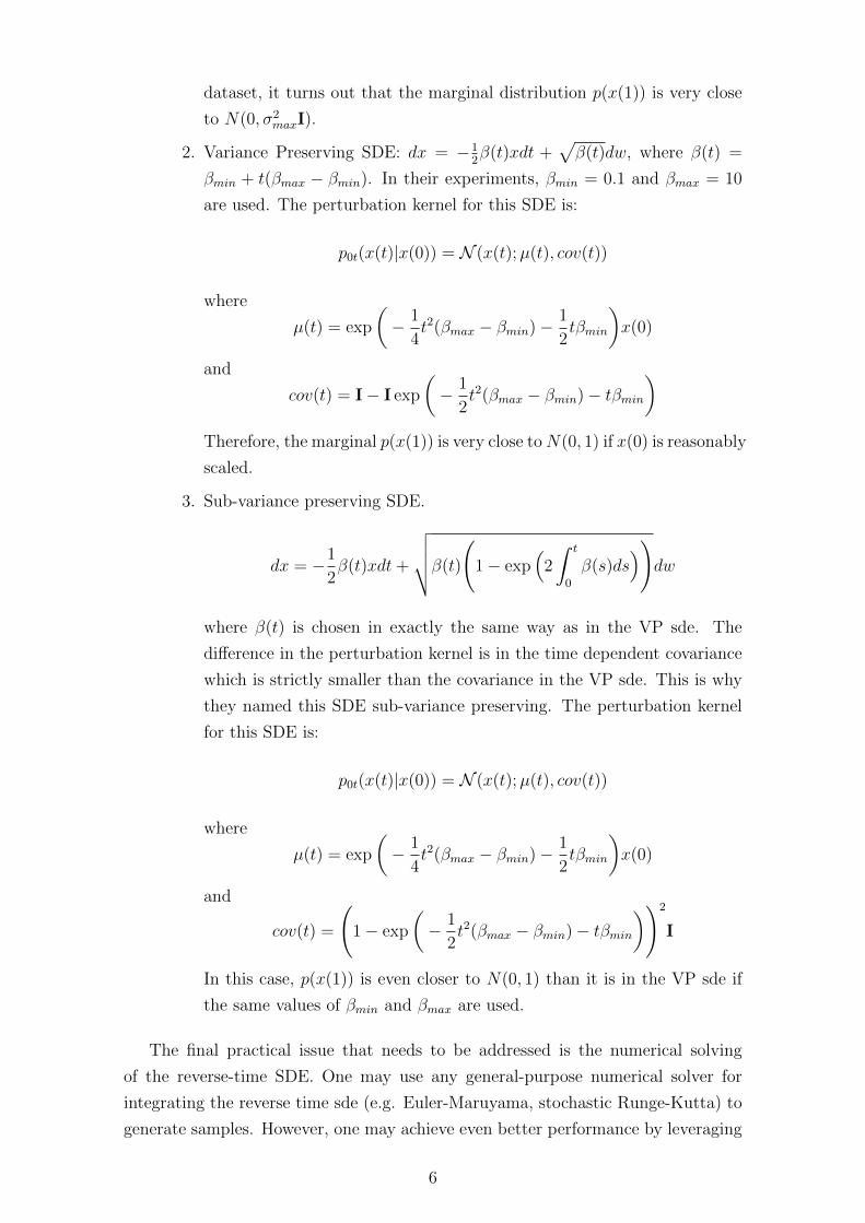
2. Variance Preserving SDE: dx = −12β(t)xdt +

√β(t)dw, where β(t) =

βmin + t(βmax − βmin). In their experiments, βmin = 0.1 and βmax = 10

are used. The perturbation kernel for this SDE is:

p0t(x(t)|x(0)) = N (x(t);µ(t), cov(t))

where

µ(t) = exp

(− 1

4t2(βmax − βmin)− 1

2tβmin

)x(0)

and

cov(t) = I− I exp

(− 1

2t2(βmax − βmin)− tβmin

)Therefore, the marginal p(x(1)) is very close toN(0, 1) if x(0) is reasonably

scaled.

3. Sub-variance preserving SDE.

dx = −1

2β(t)xdt+

√√√√β(t)

(1− exp

(2

∫ t

0

β(s)ds))

dw

where β(t) is chosen in exactly the same way as in the VP sde. The

difference in the perturbation kernel is in the time dependent covariance

which is strictly smaller than the covariance in the VP sde. This is why

they named this SDE sub-variance preserving. The perturbation kernel

for this SDE is:

p0t(x(t)|x(0)) = N (x(t);µ(t), cov(t))

where

µ(t) = exp

(− 1

4t2(βmax − βmin)− 1

2tβmin

)x(0)

and

cov(t) =

(1− exp

(− 1

2t2(βmax − βmin)− tβmin

))2

I

In this case, p(x(1)) is even closer to N(0, 1) than it is in the VP sde if

the same values of βmin and βmax are used.

The final practical issue that needs to be addressed is the numerical solving

of the reverse-time SDE. One may use any general-purpose numerical solver for

integrating the reverse time sde (e.g. Euler-Maruyama, stochastic Runge-Kutta) to

generate samples. However, one may achieve even better performance by leveraging

6

the approximation of the score of the time dependent distribution, i.e. sθ(x, t) ≈∇xlog pt(x) by employing score-based MCMC approaches such as Langevin MCMC.

To do that they propose that every estimate of the numerical solver at each reverse

time step (prediction) is followed by a step of a score-based MCMC algorithm which

corrects the marginal distribution of the estimated sample, thus playing the role of

the corrector. This hybrid sampling scheme is called predictor-corrector sampler and

typically gives better performance than predictor only sampling schemes. However,

the corrector step depends on a choice of hyper-parameters which should be tuned

for each dataset using a grid search. The proposed predictor corrector samplers for

the VE and VP sdes are shown in Algorithm 2 and Algorithm 3 respectively shown

below in Figure 1.

Figure 1: PC sampling algorithms for VE and VP reverse SDEs.

Taking all this information into consideration we re-implemented the framework

in pytorch and used the code to create a demo which shows visually how the

framework works. In the demo, we show: 1.) how forward SDE gradually modifies

P0 to PT , where PT is very close to a distribution which we know a priori PT and 2.)

how the reverse SDE gradually modifies PT to a distribution P0 which is very close

to P0. We model a two dimensional P0 distribution because it is easy to visualise

the evolution of the entire distribution. In our experimental setting we decided to

model a distribution which is a mixture of 4 Gaussians and is shown in Figure 2.

In Figure 3, we show the evolution of the distribution P0 to PT as the forward

SDE is solved from 0 to 1 on the first row, while we show the evolution of distribution

pT to p0 as the reverse SDE is solved from 1 to 0.001 on the second row. A subtle

point is that we do not integrate the forward SDE from 0 to 1, but from 0.001 to 1,

because the VE sde that we used is not defined at T = 0. The same holds for the

reverse SDE. In contrast to our expectation, we did not get better results when we

used the hybrid predictor corrector sampler. We attribute that to the fact that we

did not tune the hyperparameters of the corrector step on our dataset, but we used

the hyperparameter values of the paper. The authors tuned the hyperparameters

on the CIFAR-10 dataset, which is very different from our synthetic 2D dataset.

7

Figure 2: Target distribution P0

Figure 3: demo. First row: evolution from P0 to PT by the forward SDE. Secondrow: evolution from PT to P0 by the reverse SDE.

2.2 Extension for class conditional sample generation

The framework can be readily extended for class conditional sample generation. Our

goal is to sample from p0(x(0)|y) where y is the class condition. Using the result

from Anderson, it turns out that we can sample from p0(x(0)|y) if we sample from

pT (x(T )|y) and solve the following reverse-time SDE:

dx = [f(x, t)− g(t)2∇x(t)pt(x(t)|y)]dt+ g(t)dw (8)

Noting that

∇x(t)pt(x(t)|y) = ∇x(t)pt(x(t)) +∇x(t)pt(y|x(t))

equation (8) is transformed to:

dx =(f(x, t)− g(t)2[∇x(t)pt(x(t)) +∇x(t)pt(y|x(t))]

)dt+ g(t)dw (9)

The difference from the unconditional generation is that apart from approximating

the score of the time dependent distribution, ∇x(t)pt(x(t)), we additionally need to

approximate the gradient of the forward process, ∇x(t)pt(y|x(t)). The authors of the

8

paper claim that equation (9) can be used to solve a large family of inverse problems

if an estimate of the gradient of the forward process can be obtained. In the case

of class conditional generation where y represents a class, we can train an auxiliary

time-dependent classifier pt(y|x(t)) to obtain an estimate of the time dependent

forward process. The training samples (x(t), y) for the time-dependent classifier

are obtained by sampling a pair (x(0), y) from the dataset and then getting x(t) by

integrating the forward SDE until time t. The training loss for the auxiliary classifier

is a mixture of cross-entropy losses over uniformly sampled time steps similarly to

equation (7).

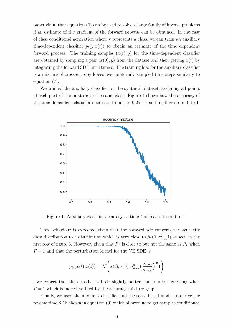
We trained the auxiliary classifier on the synthetic dataset, assigning all points

of each part of the mixture to the same class. Figure 4 shows how the accuracy of

the time-dependent classifier decreases from 1 to 0.25 + ε as time flows from 0 to 1.

Figure 4: Auxiliary classifier accuracy as time t increases from 0 to 1.

This behaviour is expected given that the forward sde converts the synthetic

data distribution to a distribution which is very close to N (0, σ2maxI) as seen in the

first row of figure 3. However, given that PT is close to but not the same as PT when

T = 1 and that the perturbation kernel for the VE SDE is

p0t(x(t)|x(0)) = N

(x(t);x(0), σ2

min

(σmaxσmin

)2tI

)

, we expect that the classifier will do slightly better than random guessing when

T = 1 which is indeed verified by the accuracy mixture graph.

Finally, we used the auxiliary classifier and the score-based model to derive the

reverse time SDE shown in equation (9) which allowed us to get samples conditioned

9

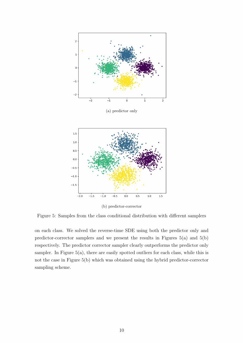
(a) predictor only

(b) predictor-corrector

Figure 5: Samples from the class conditional distribution with different samplers

on each class. We solved the reverse-time SDE using both the predictor only and

predictor-corrector samplers and we present the results in Figures 5(a) and 5(b)

respectively. The predictor corrector sampler clearly outperforms the predictor only

sampler. In Figure 5(a), there are easily spotted outliers for each class, while this is

not the case in Figure 5(b) which was obtained using the hybrid predictor-corrector

sampling scheme.

10

References

Anderson, Brian D.O. (1982). “Reverse-time diffusion equation models.” In: Stochastic

Processes and their Applications 12.3, pp. 313–326.

Kong, Zhifeng, Wei Ping, Jiaji Huang, Kexin Zhao, and Bryan Catanzaro (2020).

“DiffWave: A Versatile Diffusion Model for Audio Synthesis.” In: eprint: arXiv:

2009.09761.

Li, Xuechen, Ting-Kam Leonard Wong, Ricky T. Q. Chen, and David Duvenaud

(2020). “Scalable Gradients for Stochastic Differential Equations.” In: eprint:

arXiv:2001.01328.

Sarkka, Simo and Arno Solin (2019). Applied Stochastic Differential Equations.

Cambridge University Press. doi: 10.1017/9781108186735.

Song, Yang, Jascha Sohl-Dickstein, Diederik P. Kingma, Abhishek Kumar, Stefano

Ermon, and Ben Poole (2020). “Score-Based Generative Modeling through Stochastic

Differential Equations.” In: eprint: arXiv:2011.13456.

11