
CBC/HB v5 - Sawtooth Software€¦ · Software for Hierarchical Bayes Estimation for CBC Data...
106
Software for Hierarchical Bayes Estimation for CBC Data (Updated August 20, 2009) CBC/HB v5 Sawtooth Software, Inc. Sequim, WA http://www.sawtoothsoftware.com
-
Upload
nguyendiep -
Category
Documents
-
view
221 -
download
0
Transcript of CBC/HB v5 - Sawtooth Software€¦ · Software for Hierarchical Bayes Estimation for CBC Data...
Software for Hierarchical BayesEstimation for CBC Data
(Updated August 20, 2009)
CBC/HB v5
Sawtooth Software, Inc.Sequim, WA
http://www.sawtoothsoftware.com

Bryan Orme, Editor© Copyright 1999-2009 Sawtooth Software
In this manual, we refer to product names that are trademarked. Windows, Windows 95, Windows98, Windows 2000, Windows XP, Windows Vista, Windows NT, Excel, PowerPoint, and Word areeither registered trademarks or trademarks of Microsoft Corporation in the United States and/orother countries.

We’ve designed this manual to teach you how to use our software and to serve as a reference to answer yourquestions. If you still have questions after consulting the manual, we offer telephone support.
When you call us, please be at your computer and have at hand any instructions or files associated with yourproblem, or a description of the sequence of keystrokes or events that led to your problem. This way, we canattempt to duplicate your problem and quickly arrive at a solution.
For customer support, contact our Sequim, Washington office at 360/681-2300, email:[email protected], (fax: 360/681-2400).
Outside of the U.S., contact your Sawtooth Software representative for support.
About Technical Support

Table of Contents
Foreword
Getting Started
...................................................................................................................................................... 3Introduction
...................................................................................................................................................... 5Capacity Limitations and Hardware Recommendations
...................................................................................................................................................... 6What's New in Version 5?
Understanding the CBC/HB System
...................................................................................................................................................... 9Bayesian Analysis ...................................................................................................................................................... 12The Hierarchical Model ...................................................................................................................................................... 13Iterative Estimation of the Parameters ...................................................................................................................................................... 14The Metropolis Hastings Algorithm
Using the CBC/HB System
...................................................................................................................................................... 17Opening and Creating New Projects
...................................................................................................................................................... 19Creating Your Own Datasets in .CSV Format
...................................................................................................................................................... 22Home Tab and Estimating Parameters
...................................................................................................................................................... 24Monitoring the Computation
...................................................................................................................................................... 27Restarting
...................................................................................................................................................... 28Data Files
...................................................................................................................................................... 30Attribute Information
...................................................................................................................................................... 33Choice Task Filter
...................................................................................................................................................... 34Estimation Settings
...................................................................................................................................................... 35Iterations
...................................................................................................................................................... 37Data Coding
...................................................................................................................................................... 38Respondent Filters
...................................................................................................................................................... 39Constraints
...................................................................................................................................................... 41Utility Constraints
...................................................................................................................................................... 44Miscellaneous
...................................................................................................................................................... 45Advanced Settings
...................................................................................................................................................... 46Covariance Matrix
...................................................................................................................................................... 48Alpha Matrix
...................................................................................................................................................... 50Covariates
...................................................................................................................................................... 52Using the Results
How Good Are the Results?
...................................................................................................................................................... 53Background
...................................................................................................................................................... 54A Close Look at CBC/HB Results
References
...................................................................................................................................................... 57References
Appendices
...................................................................................................................................................... 59Appendix A: File Formats
...................................................................................................................................................... 62Appendix B: Computational Procedures
...................................................................................................................................................... 64Appendix C: .CHO and .CHS Formats
...................................................................................................................................................... 69Appendix D: Directly Specifying Design Codes in the .CHO or .CHS Files
...................................................................................................................................................... 72Appendix E: Analyzing Alternative-Specific and Partial-Profile Designs
...................................................................................................................................................... 74Appendix F: How Constant Sum Data Are Treated in CBC/HB
...................................................................................................................................................... 77Appendix G: How CBC/HB Computes the Prior Covariance Matrix
...................................................................................................................................................... 80Appendix H: Generating a .CHS File
...................................................................................................................................................... 81Appendix I: Utility Constraints for Attributes Involved in Interactions
...................................................................................................................................................... 83Appendix J: Estimation for Dual-Response "None"
...................................................................................................................................................... 85Appendix K: Estimation for MaxDiff Experiments
...................................................................................................................................................... 89Appendix L: Hardware Recommendations
...................................................................................................................................................... 90Appendix M: Calibrating Part-Worths for Purchase Likelihood
...................................................................................................................................................... 92Appendix N: Scripting in CBC/HB
Index 99

Foreword 1
1 ForewordThis Windows version of the hierarchical Bayes choice-based conjoint module fits in the best traditionof what we have come to expect from Sawtooth Software. From its inception, Sawtooth Software hasdeveloped marketing research systems that combine appropriate ways to collect information withadvanced methods of analysis and presentation. Their products also have been remarkably user-friendly in guiding managers to generate useful, managerially relevant studies. One of the reasons fortheir success is that their programs encompass the wisdom generated by the research communitygenerally and a very active Sawtooth users group.
In the case of hierarchical Bayes, Sawtooth Software has led in offering state-of-art benefits in a simpleeasy-to-use package. Hierarchical Bayes allows the marketing researcher to estimate parameters atthe individual level with less than 12 choices per person. This provides an enormous value to thosewho leverage these partworth values for segmentation, targeting and the building of what-ifsimulations. Other methods that build individual choice models were tested, and indeed offered bySawtooth Software. Latent class provided a good way to deal with heterogeneity, and SawtoothSoftware's ICE (Individual Choice Estimation) generated individual estimates from that base. However,in tests, hierarchical Bayes has proven more stable and more accurate in predicting both the itemchosen and the choice shares. This benefit occurs because conditioning a person's actual choice bythe aggregate distribution of preferences leads to better choice predictions, and that a distribution ofcoefficients for each individual is both more realistic and more informative than a point estimate.
Thus, as choice based conjoint becomes increasingly popular, this CBC/HB System provides a way forthe marketing research community to have it both ways-to combine the validity of a choice-based taskwith ease and flexibility of individual level analysis marketing researchers have long valued intraditional conjoint.
--Joel Huber, Duke University

CBC/HB v52

Getting Started 3
2 Getting Started
2.1 IntroductionThe CBC/HB System is software for estimating part worths for Choice-Based Conjoint (CBC)questionnaires. It can use either discrete choice or constant sum (chip) allocations among alternativesin choice sets. Other advanced options include the ability to estimate first-order interactions, linearterms, and covariates in the upper-level model.
CBC/HB uses data files that can be automatically exported from Sawtooth Software's CBC orCBC/Web systems. It can also use data collected in other ways, so long as the data conform to theconventions of the text-only format files, as described in the appendices of this manual.
Quick Start Instructions:
1. Prepare the .CHO or .CHS file that contains choice data to be analyzed.
a. From CBC/Web (SSI Web System), select File | Export Data andchoose the .CHO or .CHS options.
b. From ACBC (Adaptive CBC), select File | Export Data and choose the.CHO option.
2. Start CBC/HB, by clicking Start | Programs | Sawtooth Software |Sawtooth Software CBC/HB.
3. From the CBC/HB Project Wizard (or using File | Open) browse to the foldercontaining a .CHO file, and click Continue. (Wait a few moments for CBC/HB toread the file and prepare to perform analysis.)
4. To perform a default HB estimation, click Estimate Parameters Now....When complete, a file containing the individual-level part worths calledstudyname_utilities.CSV (easily opened with Excel) is saved to the same folderas your original data file. A text-only file named studyname.HBU is also createdwith the same information. If using the HB utilities in the market simulator(SMRT software), within SMRT click Analysis | Run Manager | Import andbrowse to the studyname.HBU.
The earliest methods for analyzing choice-based conjoint data (e.g. the 70s and 80s) usually did so bycombining data across individuals. Although many researchers realized that aggregate analyses couldobscure important aspects of the data, methods for estimating robust individual-level part-worth utilitiesusing a reasonable number of choice sets didn't become available until the 90s.
The Latent Class Segmentation Module was offered as the first add-on to CBC in the mid-90s,permitting the discovery of groups of individuals who respond similarly to choice questions.
Landmark articles by Allenby and Ginter (1995) and Lenk, DeSarbo, Green, and Young (1996)described the estimation of individual part worths using Hierarchical Bayes (HB) models. Thisapproach seemed extremely promising, since it could estimate reasonable individual part worths evenwith relatively little data from each respondent. However, it was very intensive computationally. Thefirst applications required as much as two weeks of computational effort, using the most powerfulcomputers available to early academics!
In 1997 Sawtooth Software introduced the ICE Module for Individual Choice Estimation, which also

CBC/HB v54
permitted the estimation of part worths for individuals, and was much faster than HB. In a 1997 paperdescribing ICE, we compared ICE solutions to those of HB, observing:
"In the next few years computers may become fast enough that Hierarchical Bayes becomesthe method of choice; but until that time, ICE may be the best method available for other thanvery small data sets."
Over the next few years, computers indeed became faster, and our CBC/HB software soon couldhandle even relatively large-sized problems in an hour or less. Today, most datasets will take about 15minutes or less for HB estimation.
HB has been described favorably in many journal articles. Its strongest point of differentiation is itsability to provide estimates of individual part worths given only a few choices by each individual. It doesthis by "borrowing" information from population information (means and covariances) describing thepreferences of other respondents in the same dataset. Although ICE also makes use of informationfrom other individuals, HB does so more effectively, and requires fewer choices from each individual.
Latent Class analysis is also a valuable method for analyzing choice data. Because Latent Class canidentify segments of respondents with similar preferences, it is an additional valuable method. Recentresearch suggests that default HB is actually faster for researchers to use than LC, when oneconsiders the decisions that should be made to fine-tune Latent Class models and select anappropriate number of classes to use (McCullough 2009).
Our software estimates an HB model using a Monte Carlo Markov Chain algorithm. In the material thatfollows we describe the HB model and the estimation process. We also provide timing estimates, aswell as suggestions about when the CBC/HB System may be most appropriate.
We at Sawtooth Software are not experts in Bayesian data analysis. In producing this software wehave been helped by several sources listed in the References. We have benefited particularly from thematerials provided by Professor Greg Allenby in connection with his tutorials at the American MarketingAssociation's Advanced Research Technique Forum, and from correspondences with Professor PeterLenk.

Getting Started 5
2.2
Capacity Limitations and HardwareRecommendationsBecause we anticipate that the CBC/HB System may be used to analyze data from sources other thanour CBC or CBC/Web software programs, it can handle data sets that are larger than the limitsimposed by CBC questionnaires. The CBC/HB System has these limitations:
· The maximum number of parameters to be estimated for any individual is 1000.
· The maximum number of alternatives in any choice task is 1000.
· The maximum number of conjoint attributes is 1000.
· The maximum number of levels in any attribute is 1000.
· The maximum number of tasks for any one respondent is 1000.
The CBC/HB System requires a fast computer and a generous amount of storage space, as offered bymost every PC that can be purchased today. By today's standards, a PC with a 2.8 GHz processor,2GB RAM, and 200 GBytes of storage space is very adequate to run CBC/HB for most problems.
There is a great deal of activity writing to the hard disk and reading back from it, which is greatlyfacilitated by Windows' ability to use extra RAM as a disk cache. The availability of RAM may thereforebe almost as critical as sheer processor speed. See Appendix L for more information.
CBC/HB v56
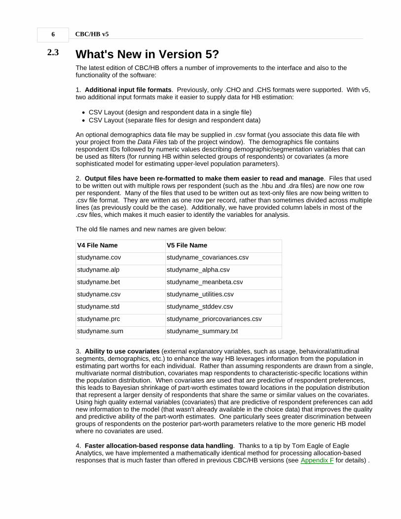
2.3 What's New in Version 5?The latest edition of CBC/HB offers a number of improvements to the interface and also to thefunctionality of the software:
1. Additional input file formats. Previously, only .CHO and .CHS formats were supported. With v5,two additional input formats make it easier to supply data for HB estimation:
· CSV Layout (design and respondent data in a single file)· CSV Layout (separate files for design and respondent data)
An optional demographics data file may be supplied in .csv format (you associate this data file withyour project from the Data Files tab of the project window). The demographics file containsrespondent IDs followed by numeric values describing demographic/segmentation variables that canbe used as filters (for running HB within selected groups of respondents) or covariates (a moresophisticated model for estimating upper-level population parameters).
2. Output files have been re-formatted to make them easier to read and manage. Files that usedto be written out with multiple rows per respondent (such as the .hbu and .dra files) are now one rowper respondent. Many of the files that used to be written out as text-only files are now being written to.csv file format. They are written as one row per record, rather than sometimes divided across multiplelines (as previously could be the case). Additionally, we have provided column labels in most of the.csv files, which makes it much easier to identify the variables for analysis.
The old file names and new names are given below:
V4 File Name V5 File Name
studyname.cov studyname_covariances.csv
studyname.alp studyname_alpha.csv
studyname.bet studyname_meanbeta.csv
studyname.csv studyname_utilities.csv
studyname.std studyname_stddev.csv
studyname.prc studyname_priorcovariances.csv
studyname.sum studyname_summary.txt
3. Ability to use covariates (external explanatory variables, such as usage, behavioral/attitudinalsegments, demographics, etc.) to enhance the way HB leverages information from the population inestimating part worths for each individual. Rather than assuming respondents are drawn from a single,multivariate normal distribution, covariates map respondents to characteristic-specific locations withinthe population distribution. When covariates are used that are predictive of respondent preferences,this leads to Bayesian shrinkage of part-worth estimates toward locations in the population distributionthat represent a larger density of respondents that share the same or similar values on the covariates.Using high quality external variables (covariates) that are predictive of respondent preferences can addnew information to the model (that wasn't already available in the choice data) that improves the qualityand predictive ability of the part-worth estimates. One particularly sees greater discrimination betweengroups of respondents on the posterior part-worth parameters relative to the more generic HB modelwhere no covariates are used.
4. Faster allocation-based response data handling. Thanks to a tip by Tom Eagle of EagleAnalytics, we have implemented a mathematically identical method for processing allocation-basedresponses that is much faster than offered in previous CBC/HB versions (see Appendix F for details) .
Getting Started 7
We've tried v5 on three small-to-moderate sized allocation-based CBC data sets we have in the office,and get between a 33% to 80% increase in speed over version 4, depending on the data set.
5. Calibration tool for rescaling utilities to predict stated purchase likelihood (purchaselikelihood model). Some researchers include ratings-based purchase likelihood questions (forconcepts considered one-at-a-time) alongside their CBC surveys (similar to those in the ACA system).The calibration routine is used for rescaling part-worths to be used in the Purchase Likelihoodsimulation model offered in Sawtooth Software's market simulator. It rescales the part-worths (bymultiplying them by a slope and adding an intercept) so they provide a least-squares fit to statedpurchase likelihoods of product concepts. The calibration tool is available from the Tools menu ofCBC/HB v5.
6. 64-bit processing supported. If you have 64-bit processing for your computer configuration,CBC/HB v5 takes advantage of that for faster run times.
7. Ability to specify prior alpha mean and variance. By default, the mean prior alpha (populationpart-worth estimates) is 0 and prior variance was infinity in past versions of the software. Advancedusers may now change those settings. However, we have seen that they have little effect on theposterior estimates. This may only be of interest for advanced users who want CBC/HB to perform asclose as possible to HB runs done in other software.
8. Ability to create projects using scripts run from the command line or an external programsuch as Excel. You can set up projects, set control values, and submit runs through a scriptingprotocol. This is useful if automating HB runs and project management.

CBC/HB v58

Understanding the CBC/HB System 9
3 Understanding the CBC/HB System
3.1 Bayesian AnalysisThis section attempts to provide an intuitive understanding of the Hierarchical Bayes method asapplied to the estimation of conjoint part worths. For those desiring a more rigorous treatment, wesuggest "Bayesian Data Analysis" (1996) by Gelman, Carlin, Stern, and Rubin.
Bayesian Analysis
In statistical analysis we consider three kinds of concepts: data, models, and parameters.
· In our context, data are the choices that individuals make.
· Models are assumptions that we make about data. For example, we may assume that adistribution of data is normally distributed, or that variable y depends on variable x, but not onvariable z.
· Parameters are numerical values that we use in models. For example, we might say that aparticular variable is normally distributed with mean of 0 and standard deviation of 1. Thosevalues are parameters.
Often in conventional (non-Bayesian) statistical analyses, we assume that our data are described by aparticular model with specified parameters, and then we investigate whether the data are consistentwith those assumptions. In doing this we usually investigate the probability distribution of the data,given the assumptions embodied in our model and its parameters.
In Bayesian statistical analyses, we turn this process around. We again assume that our data aredescribed by a particular model and do a computation to see if the data are consistent with thoseassumptions. But in Bayesian analysis, we investigate the probability distribution of the parameters,given the data. To illustrate this idea we review a few concepts from probability theory. We designatethe probability of an event A by the notation p(A), the probability of an event B by the notation p(B), andthe joint probability of both A and B by the notation p(A,B).
Bayesian analysis makes much use of conditional probability. Feller (1957) illustrates conditionalprobability with an example of sex and colorblindness. Suppose we select an individual at randomfrom a population. Let A indicate the event of that individual being colorblind, and let B indicate theevent of that individual being female. If we were to do many such random draws, we could estimatethe probability of a person being both female and colorblind by counting the proportion of individualsfound to be both females and colorblind in those draws.
We could estimate the probability of a female's being colorblind by dividing the number of colorblindfemales obtained by the number of females obtained. We refer to such a probability as "conditional;" inthis case the probability of a person being colorblind is conditioned by the person being female. Wedesignate the probability of a female's being colorblind by the symbol p(A|B), which is defined by theformula:
p(A|B) = p(A,B) / p(B).
That is to say, the probability an individual's being colorblind, given that she is female, is equal to theprobability of the individual being both female and colorblind, divided by the probability of being female.
Notice that we can multiply both sides of the above equation by the quantity p(B) to obtain an alternateform of the same relationship among the quantities:
p(A|B) p(B) = p(A,B).

CBC/HB v510
We may write a similar equation in which the roles of A and B are reversed:
p(B|A) p(A) = p(B,A).
and, since the event (B,A) is the same as the event (A,B), we may also write:
p(B|A) p(A) = p(A,B).
The last equation will be used as the model for a similar one below.
Although concrete concepts such as sex and colorblindness are useful for reviewing the concepts ofprobability, it is helpful to generalize our example a little further to illustrate what is known as "Bayestheorem." Suppose we have a set of data that we represent by the symbol y, and we consideralternative hypotheses about parameters for a model describing those data, which we represent withthe symbols Hi, with i = 1, 2, ….
We assume that exactly one of those alternative hypotheses is true. The hypotheses could be any setof mutually exclusive conditions, such as the assumption that an individual is male or female, or thathis/her age falls in any of a specific set of categories.
Rather than expressing the probability of the data given a hypothesis, Bayes' theorem expresses theprobability of a particular hypothesis, Hi , given the data. Using the above definition of conditionalprobability we can write
p(Hi | y) = p(Hi , y) / p(y).
But we have already seen (two equations earlier) that:
p(Hi , y) = p(y | Hi ) p(Hi )
Substituting this equation in the previous one, we get
p(Hi | y) = p(y | Hi ) p(Hi ) / p(y)
Since we have specified that exactly one of the hypotheses is true, the sum of their probabilities isunity. The p(y) in the denominator, which does not depend on i, is a normalizing constant that makesthe sum of the probabilities equal to unity. We could equally well write
p(Hi | y) µ p(y | Hi ) p(Hi )
where the symbol µ means "is proportional to."
This expression for the conditional probability of a hypothesis, given the data, is an expression of"Bayes theorem," and illustrates the central principle of Bayesian analysis:
· The probability p(Hi ) of the hypothesis is known as its "prior probability," which describes ourbelief about that hypothesis before we see the data.
· The conditional probability p(y | Hi ) of the data, given the hypothesis, is known as the"likelihood" of the data, and is the probability of seeing that particular collection of values, giventhat hypothesis about the data.
· The probability p(Hi | y) of the hypothesis, given the data, is known as its "posteriorprobability." This is the probability of the hypothesis, given not only the prior information aboutits truth, but also the information contained in the data.
The posterior probability of the hypothesis is proportional to the product of the likelihood of the data

Understanding the CBC/HB System 11
under that hypothesis, times the prior probability of that hypothesis. Bayesian analysis thereforeprovides a way to update estimates of probabilities. We can start with an initial or prior estimate of theprobability of a hypothesis, update it with information from the data, and obtain a posterior estimate thatcombines the prior information with information from the data.
In the next section we describe the hierarchical model used by the CBC/HB System. Bayesianupdating of probabilities is the conceptual apparatus that allows us to estimate the parameters of thatmodel, which is why we have discussed the relationship between priors, likelihoods, and posteriorprobabilities.
In our application of Bayesian analysis, we will be dealing with continuous rather than discretedistributions. Although the underlying logic is identical, we would have to substitute integrals forsummation signs if we were to write out the equations. Fortunately, we shall not find it necessary to doso.

CBC/HB v512
3.2 The Hierarchical ModelThe Hierarchical Bayes model used by the CBC/HB System is called "hierarchical" because it has twolevels.
· At the higher level, we assume that individuals' part worths are described by a multivariatenormal distribution. Such a distribution is characterized by a vector of means and a matrix ofcovariances.
· At the lower level we assume that, given an individual's part worths, his/her probabilities ofchoosing particular alternatives are governed by a multinomial logit model.
To make this model more explicit, we define some notation. We assume individual part worths havethe multivariate normal distribution,
ßi ~ Normal(a, D)
where:
ßi = a vector of part worths for the ith individual
a = a vector of means of the distribution of individuals' part worths
D = a matrix of variances and covariances of the distribution of part worths across individuals
At the individual level, choices are described by a multinomial logit model. The probability of the ithindividual choosing the kth alternative in a particular task is
pk = exp(x
k' ß
i ) /å
j exp(x
j' ß
i )
where:
pk = the probability of an individual choosing the kth concept in a particular choice task
xj = a vector of values describing the jth alternative in that choice task
In words, this equation says that to estimate the probability of the ith person's choosing the kthalternative (by the familiar process used in many conjoint simulators) we:
1. add up the part worths (elements of ßi ) for the attribute levels describing the kth alternative
(more generally, multiply the part worths by a vector of descriptors of that alternative) toget the ith individual's utility for the kth alternative
2. exponentiate that alternative's utility
3. perform the same operations for other alternatives in that choice task, and
4. percentage the result for the kth alternative by the sum of similar values for all alternatives.
The parameters to be estimated are the vectors ßi of part worths for each individual, the vector a of
means of the distribution of worths, and the matrix D of the variances and covariances of thatdistribution.
Understanding the CBC/HB System 13
3.3 Iterative Estimation of the ParametersThe parameters ß, a, and D are estimated by an iterative process. That process is quite robust, andits results do not appear to depend on starting values. We take a conservative approach by default,setting the elements of ß, a, and D equal to zero.
Given the initial values, each iteration consists of these three steps:
· Using present estimates of the betas and D, generate a new estimate of a. We assume a isdistributed normally with mean equal to the average of the betas and covariance matrix equalto D divided by the number of respondents. A new estimate of a is drawn from that distribution(see Appendix B for details).
· Using present estimates of the betas and a, draw a new estimate of D from the inverseWishart distribution (see Appendix B for details).
· Using present estimates of a and D, generate new estimates of the betas. This is the mostinteresting part of the iteration, and we describe it in the next section. A procedure known as a"Metropolis Hastings Algorithm" is used to draw the betas. Successive draws of the betasgenerally provide better and better fit of the model to the data, until such time as increases areno longer possible. When that occurs we consider the iterative process to have converged.
In each of these steps we re-estimate one set of parameters (a, D or the betas) conditionally, givencurrent values for the other two sets. This technique is known as "Gibbs sampling," and converges tothe correct distributions for each of the three sets of parameters.
Another name for this procedure is a "Monte Carlo Markov Chain," deriving from the fact that theestimates in each iteration are determined from those of the previous iteration by a constant set ofprobabilistic transition rules. This Markov property assures that the iterative process converges.
This process is continued for a large number of iterations, typically several thousand or more. After weare confident of convergence, the process is continued for many further iterations, and the actualdraws of beta for each individual as well as estimates of a and D are saved to the hard disk. The finalvalues of the part worths for each individual, and also of a and D, are obtained by averaging the valuesthat have been saved.
CBC/HB v514
3.4 The Metropolis Hastings AlgorithmWe now describe the procedure used to draw each new set of betas, done for each respondent in turn.We use the symbol ß
o (for "beta old") to indicate the previous iteration's estimation of an individual's
part worths. We generate a trial value for the new estimate, which we shall indicate as ßn (for "beta
new"), and then test whether it represents an improvement. If so, we accept it as our next estimate. Ifnot, we accept or reject it with probability depending on how much worse it is than the previousestimate.
To get ßn we draw a random vector d of "differences" from a distribution with mean of zero and
covariance matrix proportional to D, and let ßn = ß
o+ d.
We calculate the probability of the data (or "likelihood") given each set of part worths, ßo and ß
n, using
the formula for the logit model given above. That is done by calculating the probability of each choicethat individual made, using the logit formula for pk described in the previous section, and thenmultiplying all those probabilities together.
Call the resulting values po and p
n respectively.
We also calculate the relative density of the distribution of the betas corresponding to ßo and ß
n, given
current estimates of parameters a and D (that serve as "priors" in the Bayesian updating). Call thesevalues d
o and
d
n, respectively. The relative density of the distribution at the location of a point ß is
given by the formula
Relative Density = exp[-1/2(ß - a)' D-1[(ß - a)]
Finally we then calculate the ratio:
r = pn d
n / p
o d
o
Recall from the discussion of Bayesian updating that the posterior probabilities are proportional to theproduct of the likelihoods times the priors. The probabilities p
n and p
o are the likelihoods of the data
given parameter estimates ßn and ß
o, respectively. The densities d
n and d
o are proportional to the
probabilities of drawing those values of ßn and ß
o, respectively, from the distribution of part worths, and
play the role of priors. Therefore, r is the ratio of posterior probabilities of those two estimates of beta,given current estimates of a and D, as well as information from the data.
If r is greater than or equal to unity, ßn has posterior probability greater than or equal to that of ß
o, and
we accept ßn as our next estimate of beta for that individual. If r is less than unity, then ß
n has
posterior probability less than that of ßo. In that case we use a random process to decide whether to
accept ßn or retain ß
o for at least one more iteration. We accept ß
n with probability equal to r.
As can be seen, two influences are at work in deciding whether to accept the new estimate of beta. If itfits the data much better than the old estimate, then p
n will be much larger than p
o, which will tend to
produce a larger ratio. However, the relative densities of the two candidates also enter into thecomputation, and if one of them has a higher density with respect to the current estimates of a and D,then that candidate has an advantage.
If the densities were not considered, then betas would be chosen solely to maximize likelihoods. Thiswould be similar to conducting logit estimation for each individual separately, and eventually the betasfor each individual would converge to values that best fit his/her data, without respect to any higher-level distribution. However, since densities are considered, and estimates of the higher-leveldistribution change with each iteration, there is considerable variation from iteration to iteration. Evenafter the process has converged, successive estimations of the betas are still quite different from oneanother. Those differences contain information about the amount of random variation in eachindividual's part worths that best characterizes them.
Understanding the CBC/HB System 15
We mentioned that the vector d of differences is drawn from a distribution with mean of zero andcovariance matrix proportional to D, but we did not specify the proportionality factor. In the literature,the distribution from which d is chosen is called the "jumping distribution," because it determines thesize of the random jump from ß
o to ß
n. This scale factor must be chosen well because the speed of
convergence depends on it. Jumps that are too large are unlikely to be accepted, and those that aretoo small will cause slow convergence.
Gelman, Carlin, Stern, and Rubin (p 335) state: "A Metropolis algorithm can also be characterized bythe proportion of jumps that are accepted. For the multivariate normal distribution, the optimal jumpingrule has acceptance rate around 0.44 in one dimension, declining to about 0.23 in high dimensions…This result suggests an adaptive simulation algorithm."
We employ an adaptive algorithm to adjust the average jump size, attempting to keep the acceptancerate near 0.30. The proportionality factor is arbitrarily set at 0.1 initially. For each iteration we countthe proportion of respondents for whom ß
n is accepted. If that proportion is less than 0.3, we reduce
the average jump size by ten percent. If that proportion is greater than 0.3, we increase the averagejump size by ten percent. As a result, the average acceptance rate is kept close to the target of 0.30.
The iterative process has two stages. During the first stage, while the process is moving towardconvergence, no attempt is made to save any of the results. During the second stage we assume theprocess has converged, and results for hundreds or thousands of iterations may be saved to the harddisk. For each iteration there is a separate estimate of each of the parameters. We are particularlyinterested in the betas, which are estimates of individuals' part worths. We produce point estimates foreach individual by averaging the results from many iterations. We can also estimate the variances andcovariances of the distribution of respondents by averaging results from the same iterations.
Readers with solid statistical background who are interested in further information about the MetropolisHastings Algorithm may find the article by Chib and Greenberg (1995) useful.

CBC/HB v516
Using the CBC/HB System 17
4 Using the CBC/HB System
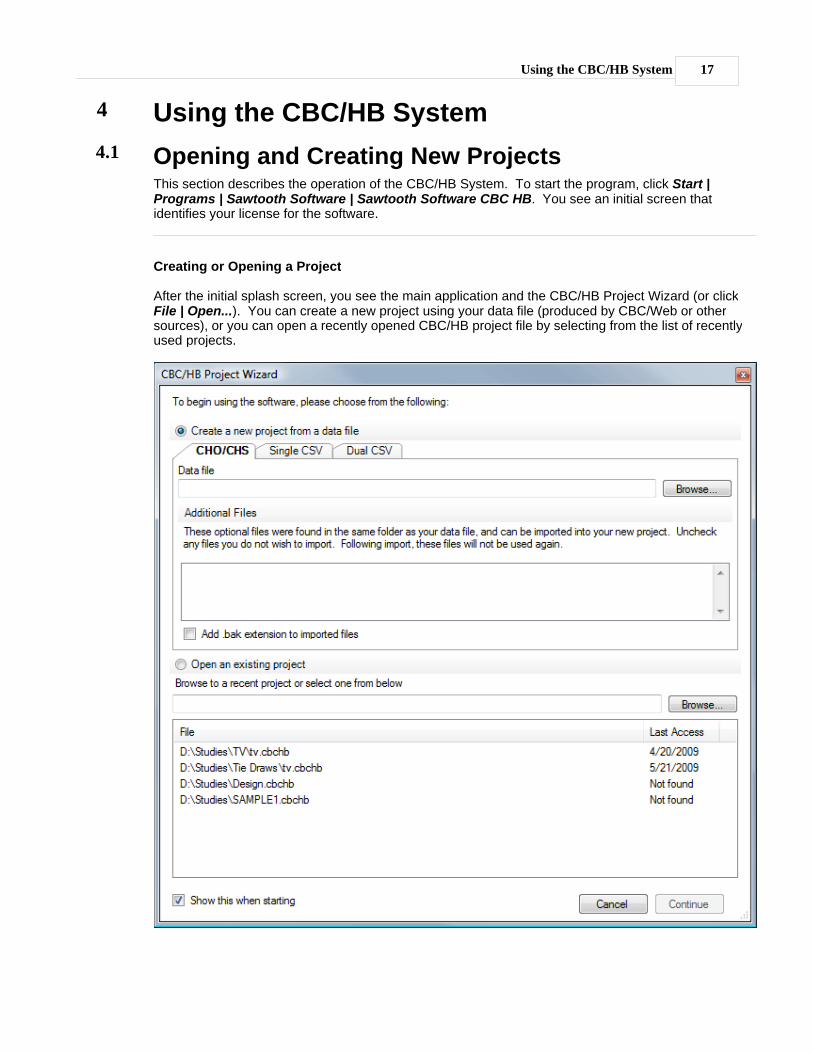
4.1 Opening and Creating New ProjectsThis section describes the operation of the CBC/HB System. To start the program, click Start |Programs | Sawtooth Software | Sawtooth Software CBC HB. You see an initial screen thatidentifies your license for the software.
Creating or Opening a Project
After the initial splash screen, you see the main application and the CBC/HB Project Wizard (or clickFile | Open...). You can create a new project using your data file (produced by CBC/Web or othersources), or you can open a recently opened CBC/HB project file by selecting from the list of recentlyused projects.
CBC/HB v518
The project wizard has the following options:
Create a new project from a data fileIf you collected CBC data using Sawtooth Software's CBC or ACBC systems, you should use SSIWeb (the platform containing those programs) to export a studyname.cho or studyname.chs file(with its accompanying labels file, called studyname.att). A studyname.cho file is a text file thatcontains information about the product concepts shown and the answers given for choose-one(standard discrete choice) tasks. A studyname.chs file is a text file that contains information aboutproduct concepts shown and answers given for allocation (constant-sum) tasks. From SSI Web,click File | Export Data | Prepare CBC Data Files to generate the studyname.cho orstudyname.chs file.
Note: If you supplied any earlier CBC/HB control files (.EFF, .VAL, .CON, .SUB, .QAL, .MTRX),these files are also available for import into your new CBC/HB project (you may uncheck any youdo not wish to import).
Open an existing projectClick this option to open an existing CBC/HB v5 project with a .cbchb extension. Projects createdwith CBC/HB v4 will be updated to the new version (NOTE: updated projects can no longer beopened with v4).
Saving the Project
Once you have opened a project using either of the methods above and have configured your desiredsettings for the HB run, you can save the project by clicking File | Save. The settings for your CBC/HBrun are saved under the name studyname.cbchb. If you want to save a copy of the project under anew name (perhaps containing different settings), click File | Save As and supply a new project (study)name. A new project is stored as newstudyname.cbchb.
Note: You may find it useful to use the File | Save As feature to create multiple project files containingdifferent project settings, but all utilizing the same data set. That way, you can submit the multiple runsin batch mode using Analysis | Batch Estimation....
Edit | View Data File
It is not necessary to know the layout of the studyname.cho or studyname.chs file to use CBC/HBeffectively. However, if you are interested, you can click the Edit | View Data File option. Anychanges you make to this file are committed to disk (after prompting you to save changes), so takecare when viewing the data file.
Using the CBC/HB System 19
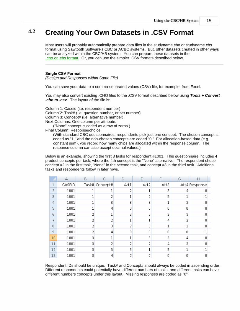
4.2 Creating Your Own Datasets in .CSV Format
Most users will probably automatically prepare data files in the studyname.cho or studyname.chsformat using Sawtooth Software's CBC or ACBC systems. But, other datasets created in other wayscan be analyzed within the CBC/HB system. You can prepare these datasets in the.cho or .chs format. Or, you can use the simpler .CSV formats described below.
Single CSV Format(Design and Responses within Same File)
You can save your data to a comma-separated values (CSV) file, for example, from Excel.
You may also convert existing .CHO files to the .CSV format described below using Tools + Convert.cho to .csv. The layout of the file is:
Column 1: Caseid (i.e. respondent number)Column 2: Task# (i.e. question number, or set number)Column 3: Concept# (i.e. alternative number)Next Columns: One column per attribute.
("None" concept is coded as a row of zeros.)Final Column: Response/choice.
(With standard CBC questionnaires, respondents pick just one concept. The chosen concept iscoded as "1," and the non-chosen concepts are coded "0." For allocation-based data (e.g.constant sum), you record how many chips are allocated within the response column. Theresponse column can also accept decimal values.)
Below is an example, showing the first 3 tasks for respondent #1001. This questionnaire includes 4product concepts per task, where the 4th concept is the "None" alternative. The respondent choseconcept #2 in the first task, "None" in the second task, and concept #3 in the third task. Additionaltasks and respondents follow in later rows.
Respondent IDs should be unique. Task# and Concept# should always be coded in ascending order.Different respondents could potentially have different numbers of tasks, and different tasks can havedifferent numbers concepts under this layout. Missing responses are coded as "0".
CBC/HB v520
By default, CBC/HB assumes each attribute column contains integer values that it will need to expandvia effects-coding (part-worth function). But, if you want to "take over" all or portions of the designmatrix and wish to specify columns that are to be used as-is (user-specified), even potentially includingdecimal values, then you may do so. You will need to identify such columns as "User-Specified"coding within CBC/HB's Attribute Information tab.
Note: Dual-Response None studies (see Appendix J) cannot be coded using the Single CSV Format.
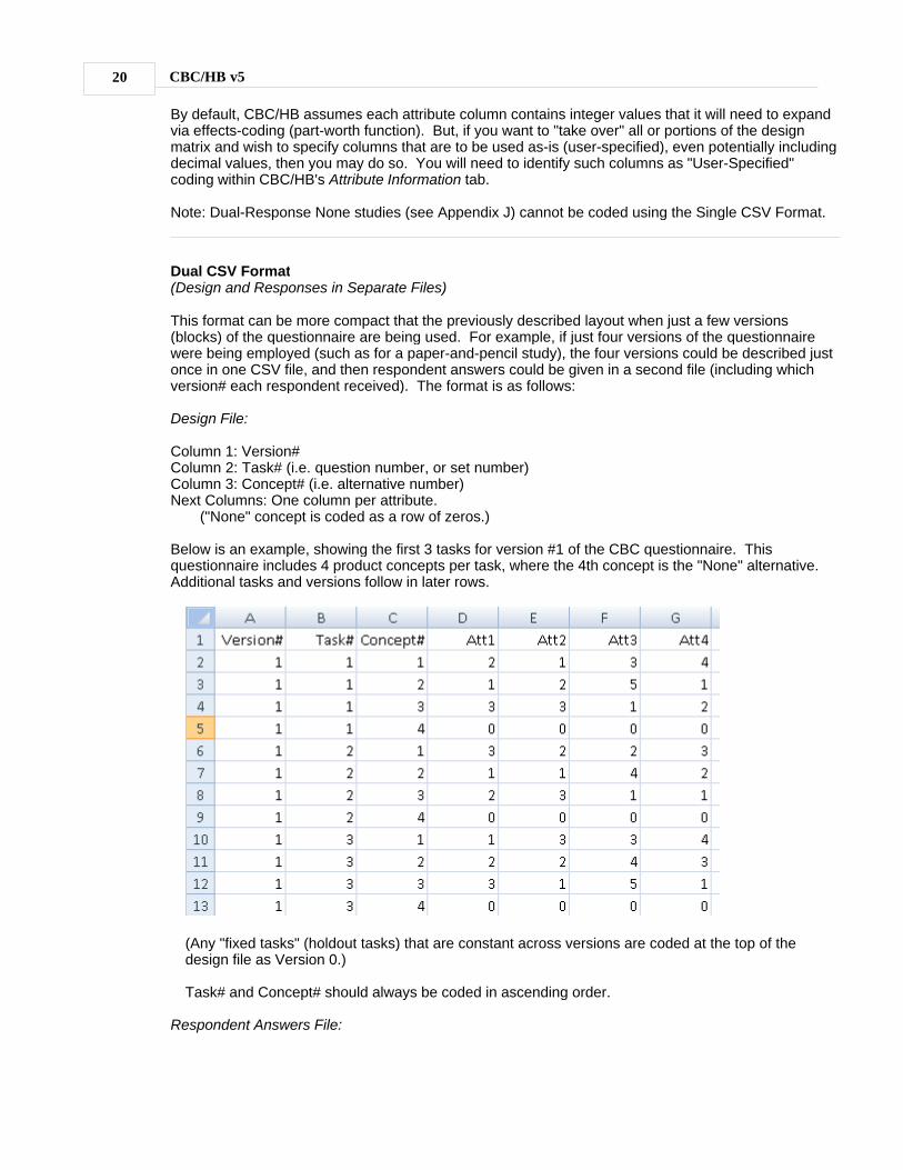
Dual CSV Format(Design and Responses in Separate Files)
This format can be more compact that the previously described layout when just a few versions(blocks) of the questionnaire are being used. For example, if just four versions of the questionnairewere being employed (such as for a paper-and-pencil study), the four versions could be described justonce in one CSV file, and then respondent answers could be given in a second file (including whichversion# each respondent received). The format is as follows:
Design File:
Column 1: Version#Column 2: Task# (i.e. question number, or set number)Column 3: Concept# (i.e. alternative number)Next Columns: One column per attribute.
("None" concept is coded as a row of zeros.)
Below is an example, showing the first 3 tasks for version #1 of the CBC questionnaire. Thisquestionnaire includes 4 product concepts per task, where the 4th concept is the "None" alternative.Additional tasks and versions follow in later rows.
(Any "fixed tasks" (holdout tasks) that are constant across versions are coded at the top of thedesign file as Version 0.)
Task# and Concept# should always be coded in ascending order.
Respondent Answers File:
Using the CBC/HB System 21
Column 1: Caseid (i.e. respondent number)Column 2: Version# (i.e. block number)Next Columns: Responses (one per task).
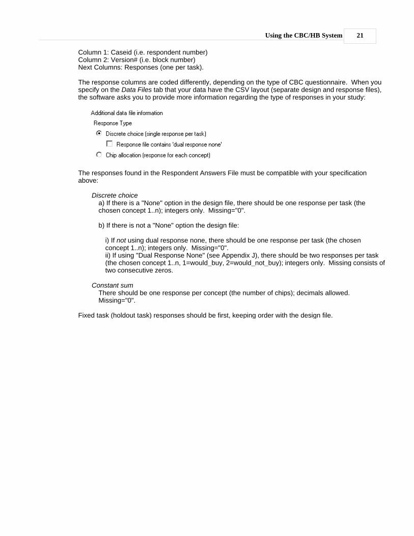
The response columns are coded differently, depending on the type of CBC questionnaire. When youspecify on the Data Files tab that your data have the CSV layout (separate design and response files),the software asks you to provide more information regarding the type of responses in your study:
The responses found in the Respondent Answers File must be compatible with your specificationabove:
Discrete choicea) If there is a "None" option in the design file, there should be one response per task (thechosen concept 1..n); integers only. Missing="0".
b) If there is not a "None" option the design file:
i) If not using dual response none, there should be one response per task (the chosenconcept 1..n); integers only. Missing="0".ii) If using "Dual Response None" (see Appendix J), there should be two responses per task(the chosen concept 1..n, 1=would_buy, 2=would_not_buy); integers only. Missing consists oftwo consecutive zeros.
Constant sumThere should be one response per concept (the number of chips); decimals allowed.Missing="0".
Fixed task (holdout task) responses should be first, keeping order with the design file.
CBC/HB v522
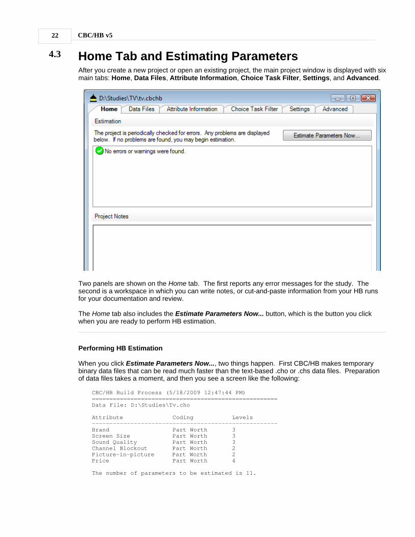
4.3 Home Tab and Estimating ParametersAfter you create a new project or open an existing project, the main project window is displayed with sixmain tabs: Home, Data Files, Attribute Information, Choice Task Filter, Settings, and Advanced.
Two panels are shown on the Home tab. The first reports any error messages for the study. Thesecond is a workspace in which you can write notes, or cut-and-paste information from your HB runsfor your documentation and review.
The Home tab also includes the Estimate Parameters Now... button, which is the button you clickwhen you are ready to perform HB estimation.
Performing HB Estimation
When you click Estimate Parameters Now..., two things happen. First CBC/HB makes temporarybinary data files that can be read much faster than the text-based .cho or .chs data files. Preparationof data files takes a moment, and then you see a screen like the following:
CBC/HB Build Process (5/18/2009 12:47:44 PM)=====================================================Data File: D:\Studies\Tv.cho
Attribute Coding Levels-----------------------------------------------------Brand Part Worth 3Screen Size Part Worth 3Sound Quality Part Worth 3Channel Blockout Part Worth 2Picture-in-picture Part Worth 2Price Part Worth 4
The number of parameters to be estimated is 11.
Using the CBC/HB System 23
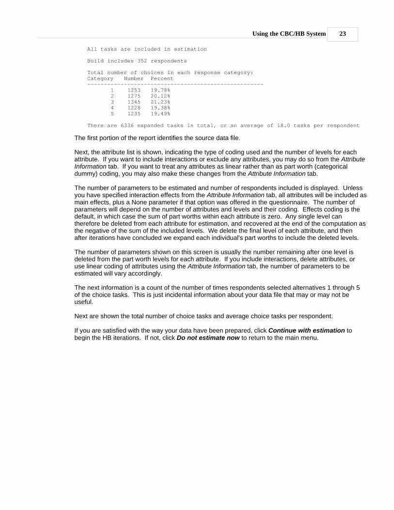
All tasks are included in estimation
Build includes 352 respondents
Total number of choices in each response category:Category Number Percent----------------------------------------------------- 1 1253 19.78% 2 1275 20.12% 3 1345 21.23% 4 1228 19.38% 5 1235 19.49%
There are 6336 expanded tasks in total, or an average of 18.0 tasks per respondent
The first portion of the report identifies the source data file.
Next, the attribute list is shown, indicating the type of coding used and the number of levels for eachattribute. If you want to include interactions or exclude any attributes, you may do so from the AttributeInformation tab. If you want to treat any attributes as linear rather than as part worth (categoricaldummy) coding, you may also make these changes from the Attribute Information tab.
The number of parameters to be estimated and number of respondents included is displayed. Unlessyou have specified interaction effects from the Attribute Information tab, all attributes will be included asmain effects, plus a None parameter if that option was offered in the questionnaire. The number ofparameters will depend on the number of attributes and levels and their coding. Effects coding is thedefault, in which case the sum of part worths within each attribute is zero. Any single level cantherefore be deleted from each attribute for estimation, and recovered at the end of the computation asthe negative of the sum of the included levels. We delete the final level of each attribute, and thenafter iterations have concluded we expand each individual's part worths to include the deleted levels.
The number of parameters shown on this screen is usually the number remaining after one level isdeleted from the part worth levels for each attribute. If you include interactions, delete attributes, oruse linear coding of attributes using the Attribute Information tab, the number of parameters to beestimated will vary accordingly.
The next information is a count of the number of times respondents selected alternatives 1 through 5of the choice tasks. This is just incidental information about your data file that may or may not beuseful.
Next are shown the total number of choice tasks and average choice tasks per respondent.
If you are satisfied with the way your data have been prepared, click Continue with estimation tobegin the HB iterations. If not, click Do not estimate now to return to the main menu.
CBC/HB v524
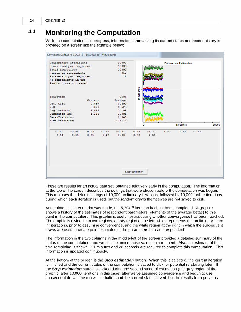
4.4 Monitoring the ComputationWhile the computation is in progress, information summarizing its current status and recent history isprovided on a screen like the example below:
These are results for an actual data set, obtained relatively early in the computation. The informationat the top of the screen describes the settings that were chosen before the computation was begun.This run uses the default settings of 10,000 preliminary iterations, followed by 10,000 further iterationsduring which each iteration is used, but the random draws themselves are not saved to disk.
At the time this screen print was made, the 5,204th iteration had just been completed. A graphicshows a history of the estimates of respondent parameters (elements of the average betas) to thispoint in the computation. This graphic is useful for assessing whether convergence has been reached.The graphic is divided into two regions, a gray region at the left, which represents the preliminary "burnin" iterations, prior to assuming convergence, and the white region at the right in which the subsequentdraws are used to create point estimates of the parameters for each respondent.
The information in the two columns in the middle-left of the screen provides a detailed summary of thestatus of the computation, and we shall examine those values in a moment. Also, an estimate of thetime remaining is shown. 11 minutes and 28 seconds are required to complete this computation. Thisinformation is updated continuously.
At the bottom of the screen is the Stop estimation button. When this is selected, the current iterationis finished and the current status of the computation is saved to disk for potential re-starting later. Ifthe Stop estimation button is clicked during the second stage of estimation (the gray region of thegraphic, after 10,000 iterations in this case) after we've assumed convergence and begun to usesubsequent draws, the run will be halted and the current status saved, but the results from previous

Using the CBC/HB System 25
iterations will be deleted. When the computation is restarted all of the iterations during which resultsare to be used will be repeated.
We now describe the statistics displayed on the screen. There are two columns for most. In the firstcolumn is the actual value for the previous iteration. The second column contains an exponentialmoving average for each statistic. At each iteration the moving average is updated with the formula:
new average = .01*(new value) + .99*(old average)
The moving average is affected by all iterations of the current session, but the most recent iterationsare weighted more heavily. The most recent 100 iterations have about 60% influence on the movingaverages, and the most recent 500 iterations have about 99% influence. Because the values in thefirst column tend to jump around quite a lot, the average values are more useful.
On the left are four statistics indicating "goodness of fit" that are useful in assessing convergence. The"Pct. Cert." and "RLH" measures are derived from the likelihood of the data. We calculate theprobability of each respondent choosing as he/she did on each task, by applying a logit model usingcurrent estimates of each respondent's part worths. The likelihood is the product of those probabilities,over all respondents and tasks. Because that probability is an extremely small number, we usuallyconsider its logarithm, which we call "log likelihood."
"Pct. Cert." is short for "percent certainty," and indicates how much better the solution is than chance,as compared to a "perfect" solution. This measure was first suggested by Hauser (1978). It is equal tothe difference between the final log likelihood and the log likelihood of a chance model, divided by thenegative of the log likelihood for a chance model. It typically varies between zero and one, with a valueof zero meaning that the model fits the data at only the chance level, and a value of one meaningperfect fit. The value of .600 for Pct. Cert. on the screen above indicates that the log likelihood is60.0% of the way between the value that would be expected by chance and the value for a perfect fit.
RLH is short for "root likelihood," and measures the goodness of fit in a similar way. To compute RLHwe simply take the nth root of the likelihood, where n is the total number of choices made by allrespondents in all tasks. RLH is therefore the geometric mean of the predicted probabilities. If therewere k alternatives in each choice task and we had no information about part worths, we would predictthat each alternative would be chosen with probability 1/k, and the corresponding RLH would also be1/k. RLH would be one if the fit were perfect. RLH has a value of .525 on the screen shown above.This data set has five alternatives per choice task, so the expected RLH value for a chance modelwould be 1/5 = .2. The actual value of .525 for this iteration would be interpreted as just better than twoand a half times the chance level.
The Pct. Cert. and RLH measures convey essentially the same information, and both are goodindicators of goodness of fit of the model to the data. The choice between them is a matter of personalpreference.
The final two statistics, "Avg Variance" and "Parameter RMS," are also indicators of goodness of fit,though less directly so. With a logit model the scaling of the part worths depends on goodness of fit:the better the fit, the larger the estimated parameters. Thus, the absolute magnitude of the parameterestimates can be used as an indirect indicator of fit. "Avg Variance" is the average of the currentestimate of the variances of part worths, across respondents. "Parameter RMS" is the root meansquare of all part worth estimates, across all part worths and over all respondents.
As iterations progress, all four values (Pct. Cert., RLH, Avg Variance, and Parameter RMS) tend toincrease for a while and then level off, thereafter oscillating randomly around their final values. Theirfailure to increase may be taken as evidence of convergence. However, there is no good way toidentify convergence until long after it has occurred. For this reason we suggest planning a largenumber of initial iterations, such as 10,000 or more, and then examining retrospectively whether thesefour measures have been stable for the last several thousand iterations.

CBC/HB v526
The studyname.log file contains a history of these measures, and may be inspected after the iterationshave concluded, or at any time during a run by clicking Stop estimation to temporarily halt the iterativeprocess. If values for the final few thousand iterations are larger than for the preceding few thousand,that should be considered as evidence that more iterations should be conducted before inferences aremade about the parameters.
At the bottom of the screen are current estimates of average part worths. The entire "expanded" vectorof part worths is displayed (up to the first 100 part worths), including the final level of each attribute thatis not counted among the parameters estimated directly.
Using the CBC/HB System 27
4.5 RestartingThe computation may be thought of as having three stages:
· The preliminary iterations before convergence is assumed, and during which iterations are notused for later analysis (the first 10,000 in the previous example)
· The final iterations, during which results are used for later analysis (the final 10,000 in theprevious example)
· If random draws are saved to disk, the time after iterations have concluded in which averagesare computed to obtain part worth estimates for each respondent and an estimate of thevariances and covariances across respondents.
During the first two stages you may halt the computation at any time by clicking Stop estimation. Thecurrent state of the computation will be saved to disk and you will later be able to restart thecomputation automatically from that point. If you click Stop estimation during the second stage, anyresults already saved or accumulated will be lost, and you will have to do more iterations to replacethose results.
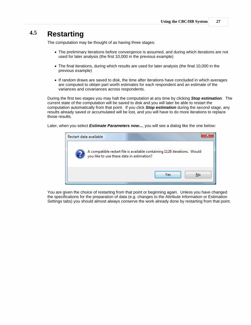
Later, when you select Estimate Parameters now..., you will see a dialog like the one below:
You are given the choice of restarting from that point or beginning again. Unless you have changedthe specifications for the preparation of data (e.g. changes to the Attribute Information or EstimationSettings tabs) you should almost always conserve the work already done by restarting from that point.

CBC/HB v528
4.6 Data Files
This tab shows you the respondent data file for your current project. A project can use data provided ina .cho or .chs file, or alternatively comma-separated values files using a single file or a combination ofdesign and response files. You can change the data file used for the current project by browsing andselecting a new one. Note: the full path to the data file is used so that multiple projects can point to it.If you move the location of your project or data file, CBC/HB may later tell you that the data file cannotbe found.
When the drop icon at the right of the Browse button is clicked, a menu appears.
You can view a quick summary of the data in the data file by clicking Summary. After a few moments,a report like the following is displayed:
Analysis of 'D:\Studies\TV\Tv.cho'Number of respondents: 352Total number of tasks: 6336Average tasks per respondent: 18Average concepts per task: 5Average attributes per concept: 6
You may view and also modify the data file by clicking View/Edit, however with large files it may beeasier to edit them with a more full-featured editor such as Notepad or Excel.

Using the CBC/HB System 29
In addition to the data file, you may specify a comma-separated values file containing demographicvariables. The variables in this file can be used as respondent filters or included as covariates inestimation. If you already have demographics in a .cho or .chs file (as "extra" values on line 2 for eachrespondent) and would like to modify them or add other data, you can select Extract Demographicsto CSV from the data file Browse button menu. This takes the extra demographic informationavailable in the .cho or .chs files and writes them to a .csv file.

CBC/HB v530
4.7 Attribute Information
The Attribute Information tab displays information about the attributes in your project, how they are tobe coded in the design file (part worth, linear, user-specified, or excluded), and whether you wish tomodel any first-order interaction effects.
Generally, most projects will require few if any modifications to the defaults on this tab. Part worth(categorical effects- or dummy-coding) estimation is the standard in the industry, and HB models oftendo not require additional first-order interaction effects to perform admirably. For illustration, in theexample above we've changed Price to be estimated as a linear function and have added aninteraction between Brand and Price.
The attribute list was created when CBC/HB initially read the data (and optional) files. If you did nothave an .att file containing labels for attributes and levels, default labels are shown. You may edit thelabels by typing or pasting text from another application. If you have somehow changed the data fileand the attribute list is no longer current, you can update it by clicking on the Other Tasks drop-downand selecting Build attribute information from data file. CBC/HB will then scan the data file toupdate the attribute information (any labels you typed in will be discarded).
The Other Tasks drop-down can also be used to change the coding of all attributes at the same time.This is helpful, for example, when using .cho files for MaxDiff studies, where all attributes need to bechanged to User Specified.
Attribute Coding
There are four options for attribute coding in CBC/HB:
Part worthThis is the standard approach used in the industry. The effect of each attribute level on choice is
Using the CBC/HB System 31
separately estimated, resulting in separate part worth utility value for each attribute level. Bydefault, CBC/HB uses effects-coding to implement part worth estimation (such that the sum ofpart-worth utilities within each attribute is zero), though you can change this to dummy coding (inwhich the final level is set to zero) on the Estimation Settings tab.
LinearWith quantitative attributes such as price or speed, some researchers prefer to fit a single linearcoefficient to model the effect of this attribute on choice. For example, suppose you have a pricevariable with 5 price levels. To estimate a linear coefficient for price, you provide a numeric valuefor each of the five levels to be used in the design matrix. This is done by selecting Linear fromthe dropdown in the Coding column. The values for each level can be typed in or pasted fromanother application into the Value column of the level list. CBC/HB always enforces zero-centeredvalues within attributes during estimation. If you do not provide values that sum to zero (withineach attribute) within this dialog, CBC/HB will subtract off the mean prior to running estimation toensure that the level values are zero-centered.
Let's assume you wish to use level values of .70, .85, 1.00, 1.15, and 1.30, which are relativevalues for 5 price levels, expressed as proportions of "normal price." You can specify those levelvalues, and CBC/HB converts them to (-0.3, -0.15, 0.0, 0.15, and 0.3) prior to estimation. If wehad used logs of the original positive values instead, then price would have been treated in theanalysis as the log of relative price (a curvi-linear function).
When specifying level values for Linear coding, you should be aware that their scaling candramatically affect the results. The range of scale values matters rather than their absolutemagnitudes, as CBC/HB automatically zero-centers the coded values for linear terms, so values of3003, 3005, and 3010 are automatically recoded as -3, -1 and +4. You should avoid using valueswith large ranges since proper convergence may only occur (especially with relatively sparse datasets) if the columns in the design matrix have similar variance. Part worth coded attributes havevalues of 1, 0 or -1 in the design matrix. For best results, we also recommend that you scale yourvalues for linear attributes such that when zero-centered, their range is about +1 to -1. That said,we have found reasonable convergence even when values have a range of five or ten. But,ranges in the hundreds or especially thousands of units or more can result in serious convergenceproblems.
Important Note: If you use Linear coding and plan to use the utilities from the HB run in SawtoothSoftware's SMRT program for running market simulations, you'll need to create a .VAL file prior toimporting the HB run into SMRT. Simply select Tools | Create VAL File. You should use thesame relative values to specify products in simulations as were coded for the HB run, otherwisethe beta (utility) coefficient will be applied inappropriately.
User-specifiedThis is an advanced option for supplying your own coding of attributes in the .CHO or .CHS file (oroptional .CSV files) for use in CBC/HB. For example, you may have additional variables to includein the model, such as dummy codes indicating whether an "end display" was displaying alongsidea shelf-display task, which called attention to a particular brand in the choice set. There are amultitude of other reasons for advanced users to specify their own coding. Please see AppendixD for more information.
User-specified coding is also used for estimating parameters for .CHO datasets produced by ourMaxDiff software. It is easiest to set all attributes to user-specified (in one step) using the OtherTasks drop-down control.
ExcludedSpecify "excluded" to exclude the attribute altogether from estimation.
CBC/HB v532
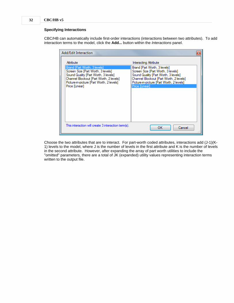
Specifying Interactions
CBC/HB can automatically include first-order interactions (interactions between two attributes). To addinteraction terms to the model, click the Add... button within the Interactions panel.
Choose the two attributes that are to interact. For part-worth coded attributes, interactions add (J-1)(K-1) levels to the model, where J is the number of levels in the first attribute and K is the number of levelsin the second attribute. However, after expanding the array of part worth utilities to include the"omitted" parameters, there are a total of JK (expanded) utility values representing interaction termswritten to the output file.

Using the CBC/HB System 33
4.8 Choice Task Filter
The Choice Task Filter tab displays a list of all available tasks in the data set. The list is automaticallygenerated when the project is created. If you have changed the data file used by your project, this listmay need updating. In that case, click the Refresh List link in the corner.
With Sawtooth Software's CBC data collection system, we often distinguish between "random" tasksand "fixed" tasks. Random tasks generally refer to those that are experimentally designed to be usedin the estimation of attribute utilities. Fixed tasks are those (such as holdout tasks) that are heldconstant across all respondents and are excluded from analysis in HB. Rather, they are used fortesting the internal validity of the resulting simulation model. The type of each task can be changed byselecting the appropriate option from the drop down. The task type has no effect on estimation -- it isavailable for your information only.
You can exclude any task by unchecking the corresponding box. Besides excluding fixed tasks, someresearchers also prefer to omit the first few choice tasks from estimation, considering them as "warm-up" tasks.
CBC/HB v534
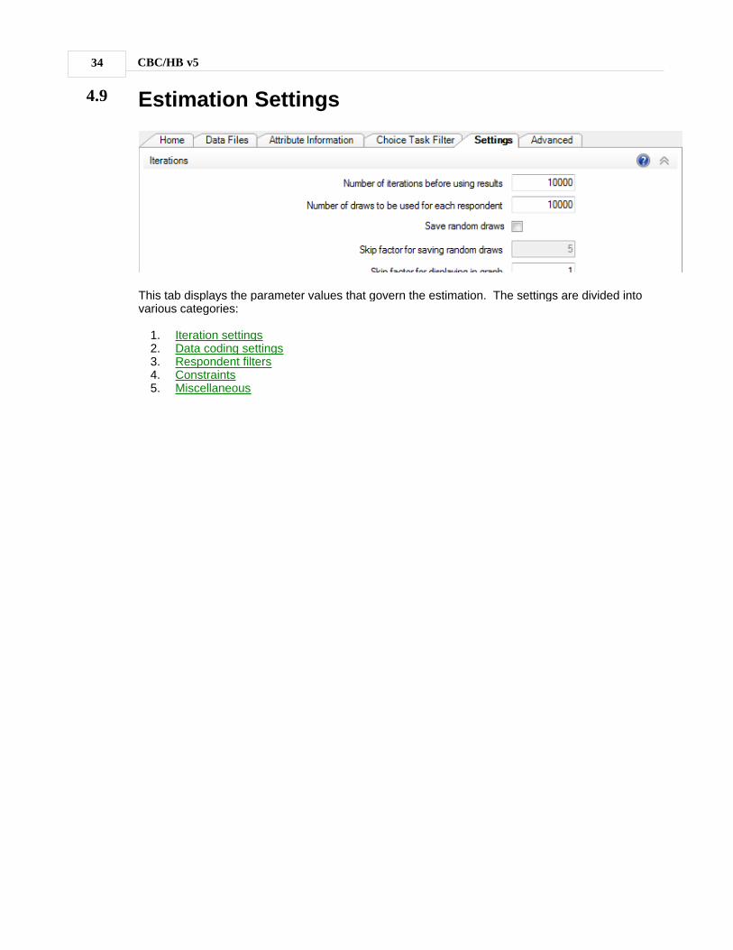
4.9 Estimation Settings
This tab displays the parameter values that govern the estimation. The settings are divided intovarious categories:
1. Iteration settings2. Data coding settings3. Respondent filters4. Constraints5. Miscellaneous

Using the CBC/HB System 35
4.9.1 Iterations
These settings determine how much information should be generated during estimation.
Number of iterations before using resultsThis determines the number of iterations that will be done before convergence is assumed.The default value is 10,000, but we have seen data sets where fewer iterations were required,and others that required many more (such as with very sparse data relative to the number ofparameters to estimate at the individual level). One strategy is to accept this default but tomonitor the progress of the computation, and halt it earlier if convergence appears to haveoccurred. Information for making that judgment is provided on the screen as the computationprogresses, and a history of the computation is saved in a file named studyname.log. Thecomputation can be halted at any time and then restarted.
Number of draws to be used for each respondentThe number of iterations used in analysis, such as for developing point estimates. If notsaving draws (described next), we recommend accumulating draws across 10,000 iterationsfor developing the point estimates. If saving draws, you may find that using more than about1,000 draws can lead to truly burdensome file sizes.
Save random drawsCheck this box to save random draws to disk, in which case final point estimates ofrespondents' betas are computed by averaging each respondent's draws after iterations havefinished. The default is not to save random draws (have the means and standard deviationsfor each respondent's draws accumulated as iteration progresses). If not saving draws themeans and standard deviations are available immediately following iterations, with no furtherprocessing. We believe that their means and standard deviations summarize almosteverything about them that is likely to be important to you.
However, if you choose to save draws to disk for further analysis, there is a trade-off betweenthe benefit of statistical precision and the time required for estimation and potential difficulty ofdealing with very large files. Consider the case of saving draws to disk. Suppose you wereestimating 25 part worths for each of 500 respondents, a "medium-sized" problem. Eachiteration would require about 50,000 bytes of hard disk storage. Saving the results for 10,000iterations would require about 500 megabytes. Approximately the same amount of additionalstorage would be required for interim results, so the entire storage requirement for even amedium-sized problem could be greater than one gigabyte.
Skip factor for saving random draws (if saving draws)This is only applicable when saving draws to disk. The skip factor is a way of compensatingfor the fact that successive draws of the betas are not independent. A skip factor of k meansthat results will only be used for each kth iteration. Recall that only about 30% of the "new"
CBC/HB v536
candidates for beta are accepted in any iteration; for the other 70% of respondents, beta is thesame for two successive iterations. This dependence among draws decreases the precisionof inferences made from them, such as their variance. If you are saving draws to disk,because file size can become critical, it makes sense to increase the independence of thedraws saved by conducting several iterations between each two for which results are saved. If1,000 draws are to be saved for each respondent and the skip factor is 10, then 10,000iterations will be required to save those 1,000 draws.
We do not skip any draws when draws are "not saved," since skipping draws to achieveindependence among them is not a concern if we are simply collapsing them to produce apoint estimate. It seems wasteful to skip draws if the user doesn't plan to separately analyzethe draws file. We have advocated using the point estimates available in the .HBU file, as webelieve that draws offer little incremental information for the purposes of running marketsimulations and summarizing respondent preferences. However, if you plan to save the drawsfile and analyze them, we suggest using a skip factor of 10. In that case, you will want to use amore practical number of draws per person (such 1,000 rather than the default 10,000 whennot saving draws), to avoid extremely large draws files.
Skip factor for displaying in graphThis controls the amount of detail that is saved in the graphical display of the history of theiterations. If using a large number of iterations (such as >50,000), graphing the iterations canrequire significant time and storage space. It is recommended in this case to increase thenumber to keep estimation running smoothly.
Skip factor for printing in log fileThis controls the amount of detail that is saved in the studyname.log file to record the history ofthe iterations. Several descriptive statistics for each iteration are printed in the log file. Butsince there may be many thousand iterations altogether, it is doubtful that you will want tobother with recording every one of them. We suggest only recording every hundredth. In thecase of a very large number of iterations, you might want to record only every thousandth.
Using the CBC/HB System 37
4.9.2 Data Coding
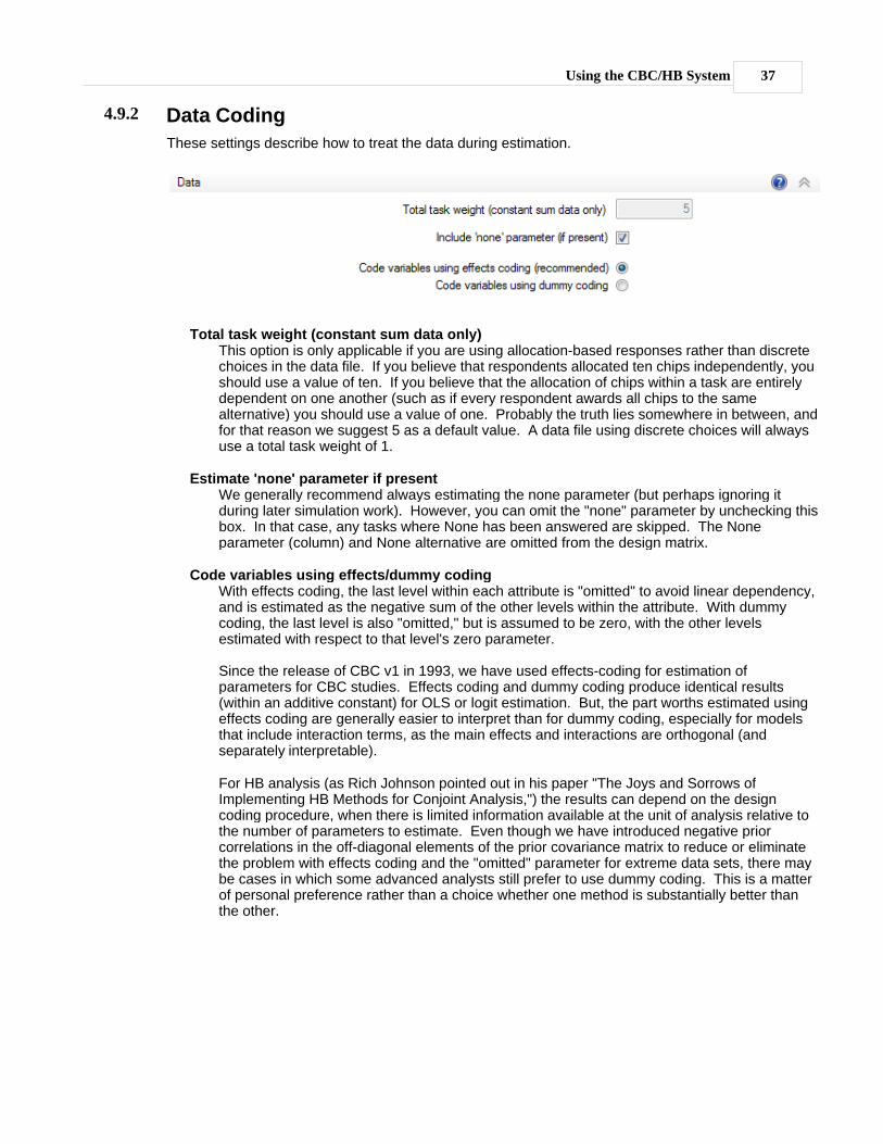
These settings describe how to treat the data during estimation.
Total task weight (constant sum data only)This option is only applicable if you are using allocation-based responses rather than discretechoices in the data file. If you believe that respondents allocated ten chips independently, youshould use a value of ten. If you believe that the allocation of chips within a task are entirelydependent on one another (such as if every respondent awards all chips to the samealternative) you should use a value of one. Probably the truth lies somewhere in between, andfor that reason we suggest 5 as a default value. A data file using discrete choices will alwaysuse a total task weight of 1.
Estimate 'none' parameter if presentWe generally recommend always estimating the none parameter (but perhaps ignoring itduring later simulation work). However, you can omit the "none" parameter by unchecking thisbox. In that case, any tasks where None has been answered are skipped. The Noneparameter (column) and None alternative are omitted from the design matrix.
Code variables using effects/dummy codingWith effects coding, the last level within each attribute is "omitted" to avoid linear dependency,and is estimated as the negative sum of the other levels within the attribute. With dummycoding, the last level is also "omitted," but is assumed to be zero, with the other levelsestimated with respect to that level's zero parameter.
Since the release of CBC v1 in 1993, we have used effects-coding for estimation ofparameters for CBC studies. Effects coding and dummy coding produce identical results(within an additive constant) for OLS or logit estimation. But, the part worths estimated usingeffects coding are generally easier to interpret than for dummy coding, especially for modelsthat include interaction terms, as the main effects and interactions are orthogonal (andseparately interpretable).
For HB analysis (as Rich Johnson pointed out in his paper "The Joys and Sorrows ofImplementing HB Methods for Conjoint Analysis,") the results can depend on the designcoding procedure, when there is limited information available at the unit of analysis relative tothe number of parameters to estimate. Even though we have introduced negative priorcorrelations in the off-diagonal elements of the prior covariance matrix to reduce or eliminatethe problem with effects coding and the "omitted" parameter for extreme data sets, there maybe cases in which some advanced analysts still prefer to use dummy coding. This is a matterof personal preference rather than a choice whether one method is substantially better thanthe other.
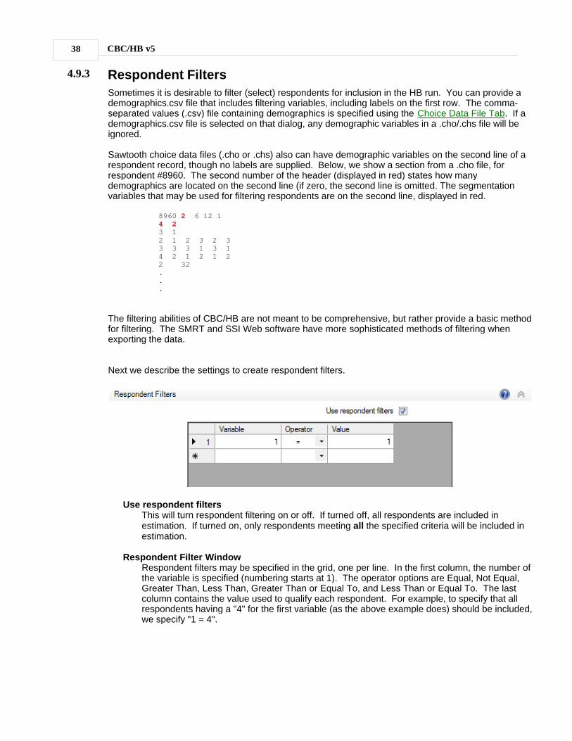
CBC/HB v538
4.9.3 Respondent Filters
Sometimes it is desirable to filter (select) respondents for inclusion in the HB run. You can provide ademographics.csv file that includes filtering variables, including labels on the first row. The comma-separated values (.csv) file containing demographics is specified using the Choice Data File Tab. If ademographics.csv file is selected on that dialog, any demographic variables in a .cho/.chs file will beignored.
Sawtooth choice data files (.cho or .chs) also can have demographic variables on the second line of arespondent record, though no labels are supplied. Below, we show a section from a .cho file, forrespondent #8960. The second number of the header (displayed in red) states how manydemographics are located on the second line (if zero, the second line is omitted. The segmentationvariables that may be used for filtering respondents are on the second line, displayed in red.
8960 2 6 12 14 23 12 1 2 3 2 33 3 3 1 3 14 2 1 2 1 22 32...
The filtering abilities of CBC/HB are not meant to be comprehensive, but rather provide a basic methodfor filtering. The SMRT and SSI Web software have more sophisticated methods of filtering whenexporting the data.
Next we describe the settings to create respondent filters.
Use respondent filtersThis will turn respondent filtering on or off. If turned off, all respondents are included inestimation. If turned on, only respondents meeting all the specified criteria will be included inestimation.
Respondent Filter WindowRespondent filters may be specified in the grid, one per line. In the first column, the number ofthe variable is specified (numbering starts at 1). The operator options are Equal, Not Equal,Greater Than, Less Than, Greater Than or Equal To, and Less Than or Equal To. The lastcolumn contains the value used to qualify each respondent. For example, to specify that allrespondents having a "4" for the first variable (as the above example does) should be included,we specify "1 = 4".
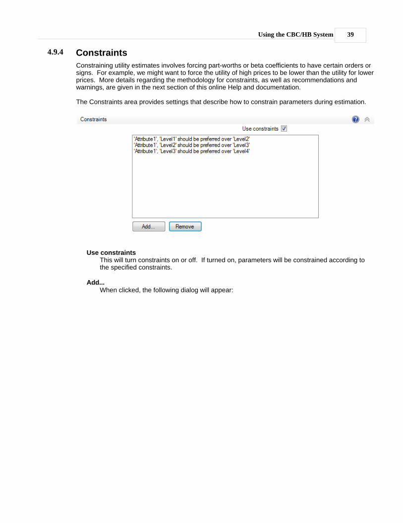
Using the CBC/HB System 39
4.9.4 Constraints
Constraining utility estimates involves forcing part-worths or beta coefficients to have certain orders orsigns. For example, we might want to force the utility of high prices to be lower than the utility for lowerprices. More details regarding the methodology for constraints, as well as recommendations andwarnings, are given in the next section of this online Help and documentation.
The Constraints area provides settings that describe how to constrain parameters during estimation.
Use constraintsThis will turn constraints on or off. If turned on, parameters will be constrained according tothe specified constraints.
Add...When clicked, the following dialog will appear:

CBC/HB v540
Constraints may be specified by selecting an attribute to constrain, and then the desiredconstraint. Part worth attributes may constrain one level to be preferred over another, or thewhole attribute can be specified to be constrained best-to-worst or worst-to-best (these optionscreate multiple constraints for all levels).
RemoveWhen one or more constraints are selected, the remove button is enabled. When clicked, theconstraints are removed permanently.
Using the CBC/HB System 41
4.9.5 Utility Constraints
Conjoint studies frequently include product attributes for which almost everyone would be expected toprefer one level to another. However, estimated part worths sometimes turn out not to have thoseexpected orders. This can be a problem, since part worths with the wrong slopes, or coefficients withthe wrong signs, are likely to yield nonsense results and can undermine users' confidence.
CBC/HB provides the capability of enforcing constraints on orders of part worths within attributes, onsigns of linear coefficients, and between coefficients from user-specified coding. The same constraintsare applied for all respondents, so constraints should only be used for attributes that haveunambiguous a-priori preference orders, such as quality, speed, price, etc.
Evidence to date suggests that constraints can be useful when the researcher is primarily interested inthe prediction of individual choices, as measured by hit rates for holdout choice tasks. However,constraints appear to be less useful, and sometimes can be harmful, if the researcher is primarilyinterested in making aggregate predictions, such as predictions of shares of choices.
Wittink (2000) pointed out that constraints can be expected to reduce variance at the expense ofincreasing bias. He observed that hit rates are sensitive to both bias and variance, so trading a largeamount of variance for a small amount of bias is likely to improve hit rates. He also observed thataggregate share predictions are mostly sensitive to bias since random error is likely to average out,and share predictions are therefore less likely to be improved by constraints.
In a paper available on the Sawtooth Software Web site (Johnson, 2000) we explored several ways ofenforcing constraints among part-worths in the HB context. Realizing that most CBC/HB users areprobably interested in predicting individual choices as well as aggregate shares, we examined thesuccess of each method with respect to both hit rates and share predictions. Two methods whichseemed most consistently successful are referred to in that paper as "Simultaneous Tying" and "TyingAfter Estimation (Tie Draws)." We have implemented both of them in CBC/HB. We call the firstmethod "Simultaneous" because it applies constraints during estimation, so the presence of theconstraints affects the estimated values. The second procedure is a less formal method of simplytying offending values of saved draws from estimation done without constraints. Although it appears towork nearly as well in practice, it has less theoretical justification.
Simultaneous Tying
This method features a change of variables between the "upper" and "lower" parts of the HB model.For the upper model, we assume that each individual has a vector of (unconstrained) part worths, withdistribution:
bi ~ Normal(a, D)where:
bi = unconstrained part worths for the ith individuala = means of the distribution of unconstrained part worthsD = variances and covariances of the distribution of unconstrained part-worths
For the lower model, we assume each individual has a set of constrained part worths, bi where bi isobtained by recursively tying each pair of elements of bi that violate the specified order constraints, andthe probability of the ith individual choosing the kth alternative in a particular task is
pk = exp(xk' bi ) /åj exp(xj' bi )
With this model, we consider two sets of part worths for each respondent: unconstrained andconstrained. The unconstrained part worths are assumed to be distributed normally in the population,
CBC/HB v542
and are used in the upper model. However, the constrained part worths are used in the lower model toevaluate likelihoods.
We speak of "recursively tying" because, if there are several levels within an attribute, tying two valuesto satisfy one constraint may lead to the violation of another. The algorithm cycles through theconstraints repeatedly until they are all satisfied.
When constraints are in force, the estimates of population means and covariances are based on theunconstrained part worths. However, since the constrained part worths are of primary interest, wereport the average of the constrained part worths on-screen, and a history of their average duringiterations is available in the studyname.meanbeta.csv file. Also, final averages of both constrainedand unconstrained part-worths as well as the unconstrained population covariances are given in thestudyname.summary.txt file.
When constraints are employed, two kinds of changes can be expected in the on-screen output:
Measures of fit (Pct. Cert. and RLH) will be decreased. Constraints always decrease the goodness-of-fit for the sample in which estimation is done. This is accepted in the hope that the constrainedsolution will work better for predictions in new choice situations.
Measures of scale (Avg. Variance and Parameter RMS), which are based on unconstrained partworths, will be increased. The constrained part worths have less variance than the unconstrained partworths, because they are produced by tying unconstrained values. Since constrained part worths areused to assess the fit of the model to the data (by computing likelihood), the constrained values takeon the "correct" scaling, and the unconstrained values therefore have greater variance.
You may impose constraints on either categorical or linear attributes.
Tying after Estimation (Tie Draws)
To use this method, select Tools | Tie Draws... after you have obtained an unconstrained HB solutionand saved random draws. The program requires the presence of studyname.hbu, andstudyname.dra files. It creates an output file named studyname_tiedraws.hbu, which is formattedlike studyname.hbu, and also creates a studyname.csv file, readable by Excel.
The TIEDRAWS utility does recursive tying of each of the random draws of part worths for eachrespondent and then averages them to get an estimate of that respondent's constrained part-worths.The program also provides an on-screen display indicating the percentage of unconstrained randomdraws for which each constraint was violated.
Simultaneous Tying often works a bit better than Tying After Estimation. This is to be expected, sincethe estimation process is informed of the constraints in Simultaneous Tying but not in Tying AfterEstimation. Simultaneous Tying also has the advantage that you can use it without having to savelarge files of random draws. However it also has a disadvantage: it requires that you specify theconstraints before estimation begins, but there may be attributes for which you don't know whether toemploy constraints or not. Doing separate HB estimations for many combinations of constraints couldtake a long time.
One way around this problem, assuming you have included "fixed" holdout choice sets in the interview,is as follows (by "fixed," we mean every respondent sees the same alternatives):
· Do unconstrained estimation, saving random draws.
· Run Tie Draws… to experiment with different constraint sets, seeing how well each predictsholdout choices and shares of choice.

Using the CBC/HB System 43
· Choose the best constraint set, and re-run the estimation using Simultaneous Tying, withoutsaving random draws.
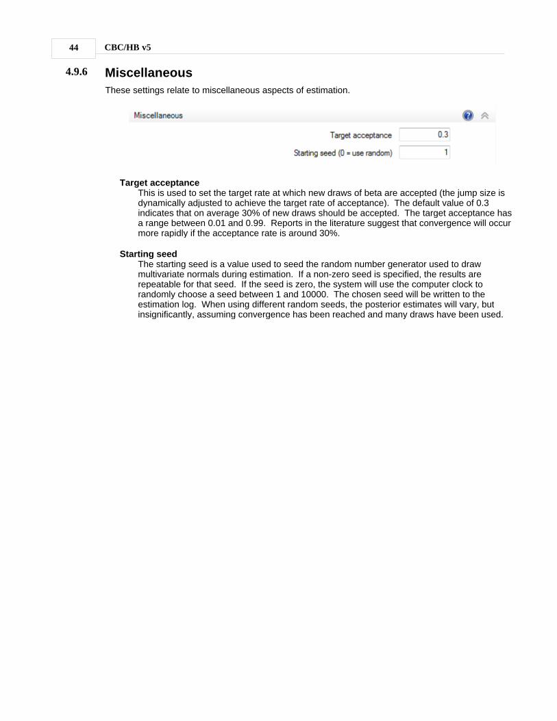
CBC/HB v544
4.9.6 Miscellaneous
These settings relate to miscellaneous aspects of estimation.
Target acceptanceThis is used to set the target rate at which new draws of beta are accepted (the jump size isdynamically adjusted to achieve the target rate of acceptance). The default value of 0.3indicates that on average 30% of new draws should be accepted. The target acceptance hasa range between 0.01 and 0.99. Reports in the literature suggest that convergence will occurmore rapidly if the acceptance rate is around 30%.
Starting seedThe starting seed is a value used to seed the random number generator used to drawmultivariate normals during estimation. If a non-zero seed is specified, the results arerepeatable for that seed. If the seed is zero, the system will use the computer clock torandomly choose a seed between 1 and 10000. The chosen seed will be written to theestimation log. When using different random seeds, the posterior estimates will vary, butinsignificantly, assuming convergence has been reached and many draws have been used.
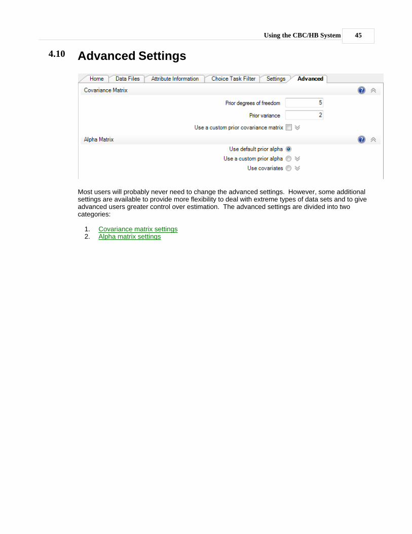
Using the CBC/HB System 45
4.10 Advanced Settings
Most users will probably never need to change the advanced settings. However, some additionalsettings are available to provide more flexibility to deal with extreme types of data sets and to giveadvanced users greater control over estimation. The advanced settings are divided into twocategories:
1. Covariance matrix settings2. Alpha matrix settings

CBC/HB v546
4.10.1 Covariance Matrix
This topic covers the covariance matrix settings in the software. See Appendix G for more informationabout the covariance matrix.
Prior degrees of freedomThis value is the additional degrees of freedom for the prior covariance matrix (not includingthe number of parameters to be estimated), and can be set from 2 to 100000. The higher thevalue, the greater the influence of the prior variance and more data are needed to change thatprior. The scaling for degrees of freedom is relative to the sample size. If you use 50 and youonly have 100 subjects, then the prior will have a big impact on the results. If you have 1000subjects, you will get about the same result if you use a prior of 5 or 50. As an example of anextreme case, with 100 respondents and a prior variance of 0.1 with prior degrees of freedomset to the number of parameters estimated plus 50, each respondent's resulting part worthswill vary relatively little from the population means. We urge users to be careful when settingthe prior degrees of freedom, as large values (relative to sample size) can make the prior exertconsiderable influence on the results.
Prior varianceThe default is 2 for the prior variance for each parameter, but users can modify this value. Youcan specify any value from 0.1 to 999. Increasing the prior variance tends to place moreweight on fitting each individual's data, and places less emphasis on "borrowing" informationfrom the population parameters. The resulting posterior estimates are relatively insensitive tothe prior variance, except 1) when there is very little information available within the unit ofanalysis relative to the number of estimated parameters, and 2) the prior degrees of freedomfor the covariance matrix (described above) is relatively large.
Use custom prior covariance matrixCBC/HB uses a prior covariance matrix that works well for standard CBC studies. Some

Using the CBC/HB System 47
advanced users may wish to specify their own prior covariance matrix (for instance, for
analysis of MaxDiff data sets). Check this box and click the icon to make the priorcovariance matrix visible. The number of parameters can be adjusted by using the up anddown arrows on the Parameters field, or you may type a number in the field. The number ofparameters needs to be the same as the number of parameters to be estimated. Values forthe matrix may be typed in or pasted from another application such as Excel. The user-specified prior covariance matrix overrides the default prior covariance matrix (see AppendixG) as well as the prior variance setting.

CBC/HB v548
4.10.2 Alpha Matrix
Most users will not change the default alpha matrix. Advanced users may specify new values for alphausing this dialog.
Covariates are a new feature with v5 of CBC/HB. More detail on the usefulness of covariates inCBC/HB is provided in the white paper, "Application of Covariates within Sawtooth Software's CBC/HBProgram: Theory and Practical Example" available for downloading from our Technical Papers libraryat www.sawtoothsoftware.com.
Use default prior alphaSelecting this option will use a default alpha matrix with prior means of zero and priorvariances of 100. No demographic variables will be used as covariates.
Use a custom prior alphaUsers can specify their own prior means and variances to be used in the alpha matrix. The
means and variances are expanded by clicking the icon.
The number of parameters for the means and variances can be adjusted by using the up anddown arrows of the Parameters field, or you may type a number in the field. The number ofparameters needs to be the same as the number of parameters to be estimated (k-1 levels perattribute, prior to utility expansion). Values for the matrix may be typed or pasted from anotherapplication such as Excel.
Use Covariates
CBC/HB v5 allows demographic variables to be used as covariates during estimation. The
available covariates can be expanded by clicking the icon.
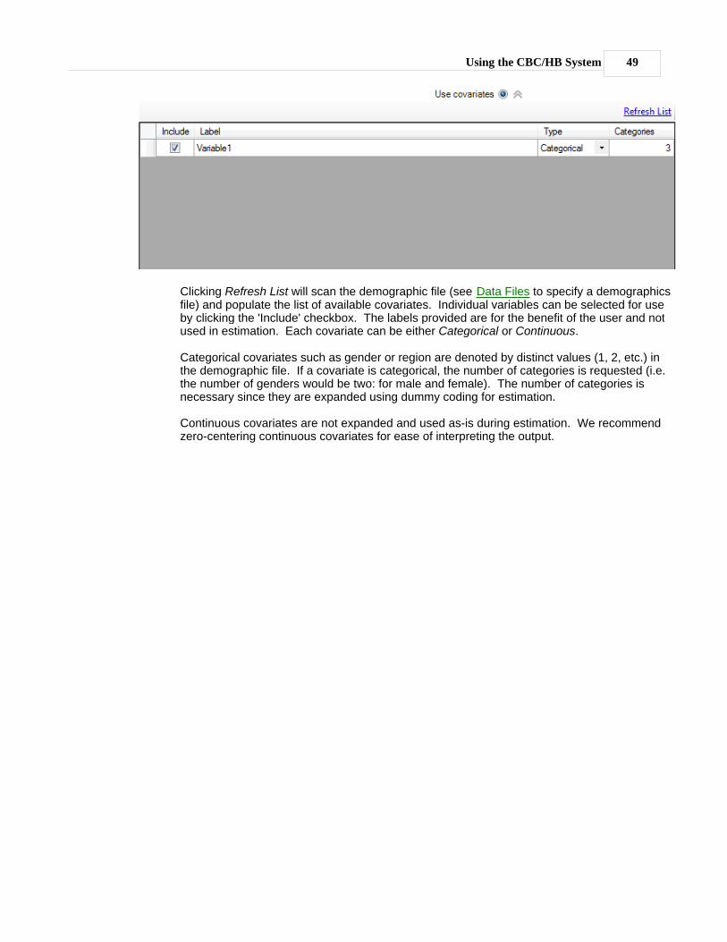
Using the CBC/HB System 49
Clicking Refresh List will scan the demographic file (see Data Files to specify a demographicsfile) and populate the list of available covariates. Individual variables can be selected for useby clicking the 'Include' checkbox. The labels provided are for the benefit of the user and notused in estimation. Each covariate can be either Categorical or Continuous.
Categorical covariates such as gender or region are denoted by distinct values (1, 2, etc.) inthe demographic file. If a covariate is categorical, the number of categories is requested (i.e.the number of genders would be two: for male and female). The number of categories isnecessary since they are expanded using dummy coding for estimation.
Continuous covariates are not expanded and used as-is during estimation. We recommendzero-centering continuous covariates for ease of interpreting the output.

CBC/HB v550
4.10.3 Covariates
Covariates are additional explanatory variables, such as usage, behavioral/attitudinal segments,demographics, etc. that can enhance the way HB leverages information from the population inestimating part worths for each individual. Rather than assuming respondents are drawn from a single,multivariate normal distribution, covariates map respondents to characteristic-specific locations withinthe population distribution. When covariates are used that are predictive of respondent preferences,this leads to Bayesian shrinkage of part-worth estimates toward locations in the population distributionthat represent a larger density of respondents that share the same or similar values on the covariates.Using high quality external variables (covariates) that are predictive of respondent preferences can addnew information to the model (that wasn't already available in the choice data) that improves the qualityand predictive ability of the part-worth estimates. One particularly sees greater discrimination betweengroups of respondents on the posterior part-worth parameters relative to the more generic HB modelwhere no covariates are used.
To use covariates, one first associates a .CSV file of demographics with the project on the Data Filestab. Respondent number must be in the first column. Covariates follow in subsequent columns.Covariates can be categorical (e.g. small_company=1, medium_company=2, large_company=3) orcontinuous (amount expect to pay for next automobile). If they are categorical, they must be recordedas consecutive integers starting with 1. Categorical covariates are coded in the Z matrix as dummy-coding, with the final level omitted as the reference zero. The covariates model is a regression-typemodel, where the population mean part-worth parameters are estimated as a function of a matrix Zdefining the respondent characteristics and a set of weights (Theta) associated with each respondentdescriptor variable.
In the example below, there are two covariates in the demographics.csv file, and the second covariate(a categorical variable with three values: 1, 2, or 3) is being used in the run.
A set of weights (Theta) associated with the intercept of the population estimates of part-worths as wellas adjustments to the population part-worth means due to characteristics of the covariates is written tothe studyname_alpha.csv file. For example, if a 3-level categorical covariate were being used, the firstcolumns of the studyname_alpha.csv file would contain estimates for each of the part-worth utilitiesassociated with the intercept of the coded covariates matrix Z (in the case of categorical coding, theintercept would be the population mean part-worth estimates associated with respondents taking onthe final level of the categorical covariate). Then, the next columns would contain of set of regressionweights (Theta) for the adjustments to the population estimates for each of the part-worth utilitiesassociated with respondents taking on the 1st level of the categorical covariate, followed by a set ofestimates for adjustments to alpha for respondents taking on the 2nd level of the categorical covariate.The columns are clearly labeled in the .CSV file. For example, if an estimate for the level "red" for

Using the CBC/HB System 51
respondents taking on characteristic 2 of Variable2 was equal to 0.75, then this would indicate thatrespondents with characteristic 2 of Variable2 had a mean part-worth utility for Red that was 0.75 utileshigher than respondents taking on characteristic 3 of Variable2 (since the final column is coded as theomitted, zero, state).
One typically examines the weights in the _alpha.csv file associated with covariates to help determinethe usefulness of the covariates. Only the "used" draws should be examined. For example, if your HBrun includes 10,000 burn-in iterations followed by 10,000 used iterations, then only the final 10,000rows of the _alpha.csv file should be examined. One can examine the mean of these draws, as wellas the percentage of the draws that are positive or negative. The means should have face validity(make sense from a behavioral standpoint, based on what you know about the respondentcharacteristics on the covariates). If the percent of draws (associated with a part-worth utility) thathave the same sign is 95% or greater, this is often taken as evidence that this realization of thecovariate has a significant effect (90% confidence level, two-tailed test) on the part-worth utilityestimate. If a relatively large number of columns for a covariate have significant weights, then thisgives evidence that the covariate is useful.
More detail on the usefulness of covariates in CBC/HB is provided in the white paper, "Application ofCovariates within Sawtooth Software's CBC/HB Program: Theory and Practical Example" available fordownloading from our Technical Papers library at www.sawtoothsoftware.com.
Note: the weights associated with a covariate within the _alpha.csv file reflect the change in the base(intercept) part-worth value when respondents take on the characteristic as described by thatcovariate. They cannot be interpreted as the part-worth utility estimate alone. Since the application ofcovariates follows a regression model, the population estimate for respondents taking on specificcovariate realizations is equal to the part-worth utility associated with the intercept plus the adjustments(weights) of the covariates associated with the respondents.
If you make changes to the demographics.csv file, you may need to click the Refresh List link to askCBC/HB to reread the demographics.csv file for use in the run.
CBC/HB v552
4.11 Using the ResultsAt the end of the computation, several files are available containing the results:
Files named studyname.hbu and studyname_utilities.csv contain final part worth estimates for eachrespondent. These are the averages of hundreds or thousands of draws either saved during the finalstage of the iterations or accumulated on the fly, if those were not saved. Thestudyname_utilities.csv file is a comma-separated text-only file that may be directly opened withExcelTM. The format of the studyname.hbu file is described in Appendix A. Either of these files,perhaps after minor modification, may be used in a conjoint simulator. If using Sawtooth Software'smarket simulator, the studyname.hbu file may directly be imported into your simulation study. If usingSMRT, you select Analysis | Run Manager | Import within SMRT's menu system.
If you have not saved random draws to disk, a file named studyname_stddev.csv contains within-respondent standard deviations for each respondent's part worths. Its format is similar to that ofstudyname.hbu.
A file named studyname_summary.txt contains summaries of the data. Its contents are slightlydifferent, depending on whether or not you have used constraints. If there were no constraints, thenthis file contains the estimated average part worths for the population of respondents, as well as thevariance-covariance matrix estimated for the population distribution. If there were constraints, then itincludes those same values for the unconstrained part worths, as well as average values for theconstrained part worths. (See the section on Constraints for further clarification.) Like the final partworth estimates, this matrix is obtained by averaging results saved during the final stage of theiterations.
A file named studyname_alpha.csv contains successive random draws of the mean of the populationdistribution. The point estimate of the average part worths for the population of respondents asreported in the studyname_summary.txt file is obtained by averaging these draws (for the range ofused draws). One way to determine when convergence occurs is to inspect this file to see whetherthere are systematic trends in any values.
If constraints were used, a file named studyname_meanbeta.csv contains successive estimates ofthe mean of the constrained betas. Like the studyname_alpha.csv file, it can be inspected todetermine when convergence occurs.
A file named studyname_covariances.csv contains successive random draws of the variances andcovariances of the population distribution. The final point estimate of the variances and covariances isobtained by averaging the draws during the final stage of the iterations. Only the elements on andabove the diagonal of the covariance matrix are saved in this file.
Finally, if you have saved random draws, a studyname.dra file is available with estimates of eachrespondent's part worths for all the iterations from which those values were saved. This may be a verylarge file, since it contains potentially thousands of estimates of part worths for each respondent. Thedata are arranged in order by respondent. This file can provide the raw data for analyses you mayundertake using statistical software packages.
How Good Are the Results? 53
5 How Good Are the Results?
5.1 BackgroundEarly articles have discussed the application of Hierarchical Bayes (HB) to the estimation of individualconjoint part worths.
· Allenby, Arora, and Ginter (1995) showed how HB could be used advantageously to introduceprior information about monotonicity constraints in individual part worths.
· In quite a different application, Allenby and Ginter (1995) showed that HB could be used toestimate individual part worths for choice data, even with relatively little data from eachrespondent.
· Lenk, DeSarbo, Green, and Young (1996) showed that HB could estimate individual part worthseffectively even when each individual provided fewer answers than the number of parametersbeing estimated.
These results were impressive, and suggested that HB might become the preferred method forestimation of individual part worths. In the past few years, this seems to have been the case.However, HB computation takes longer than methods such as latent class and logit, which led some todoubt about its feasibility in real-world applications in the mid-1990s. The Allenby and Ginter exampleused 600 respondents but estimated only 14 parameters for each. The Lenk et al. example used only179 respondents, also with 14 parameters per respondent. Many commercial applications involvemuch larger data sets. Fortunately, since then, computers have become faster, and it is now possibleto do HB estimation within a reasonable amount of time for even relatively large data sets.
CBC/HB v554
5.2 A Close Look at CBC/HB ResultsWe shall now examine CBC/HB results from a study especially designed to investigate the quality ofindividual part worth estimates. This is a data set examined by Huber et al. (1998) and we firstdescribe it in more detail.
A total of 352 respondents answered CBC questionnaires about TV preferences (this data set isavailable as a "tutorial" study within the SMRT Platform from Sawtooth Software). Each respondentanswered 18 customized choice questions consisting of 5 alternatives with no "None" option. Therewere 6 conjoint attributes having a total of 17 levels in all. The data were coded as part worths, so 17 –6 = 11 parameters were estimated for each respondent. The respondents were randomly divided intofour groups, and those in each group answered 9 holdout tasks, each with 5 alternatives. The first andeighth tasks were identical to permit an estimate of reliability. The percentage of reliable choices forthe repeated task ranged from 69% to 89%, depending on version, with an average of 81%.
The holdout tasks contained some alternatives that were very similar and sometimes identical to eachother. This was done to present a challenge to conjoint simulators based on the logit model andhaving IIA properties.
To be absolutely sure of convergence, 100,000 iterations were done with the CBC/HB System beforesaving any results. We then investigated several aspects of the estimates.
Estimation with Few Tasks
The first property examined was the ability to predict holdout choices using part worths estimated fromsmall numbers of tasks. Six sets of part worths were estimated for each respondent, based on thesenumbers of tasks: all 18, 9 even-numbered, 9 odd-numbered, 6, 4, and 2. (The last three conditionsused tasks distributed evenly throughout the questionnaire.) Each set of part worths was obtained bydoing 1000 additional HB iterations and saving results of each 10th iteration. Each set of part worthswas evaluated in two ways:
· Point estimates of each individual's part worths were obtained by averaging the 100 randomdraws, and those estimates were used in a first-choice conjoint simulator to measure hit rates.
· The random draws were also used individually in 100 separate first-choice simulations for eachrespondent, and accumulated over respondents to measure MAE (mean absolute error) inpredicting choice shares.
With first-choice simulators, adding Gumbel-distributed random error to the summed utilities flattensshare predictions in the same way that logit simulations are flattened by multiplying utilities by anumber less than unity. With Gumbel error scaled to have unit standard deviation, the optimalproportion to be added was about 0.1, and this did not differ systematically depending on the numberof tasks used in estimation. Here are the resulting Hit Rate and MAE statistics for the several sets ofpart worths:
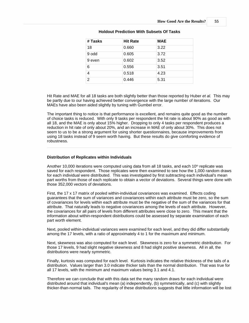
How Good Are the Results? 55
Holdout Prediction With Subsets Of Tasks
# Tasks Hit Rate MAE
18 0.660 3.22
9 odd 0.605 3.72
9 even 0.602 3.52
6 0.556 3.51
4 0.518 4.23
2 0.446 5.31
Hit Rate and MAE for all 18 tasks are both slightly better than those reported by Huber et al. This maybe partly due to our having achieved better convergence with the large number of iterations. OurMAEs have also been aided slightly by tuning with Gumbel error.
The important thing to notice is that performance is excellent, and remains quite good as the numberof choice tasks is reduced. With only 9 tasks per respondent the hit rate is about 90% as good as withall 18, and the MAE is only about 15% higher. Dropping to only 4 tasks per respondent produces areduction in hit rate of only about 20%, and an increase in MAE of only about 30%. This does notseem to us to be a strong argument for using shorter questionnaires, because improvements fromusing 18 tasks instead of 9 seem worth having. But these results do give comforting evidence ofrobustness.
Distribution of Replicates within Individuals
Another 10,000 iterations were computed using data from all 18 tasks, and each 10th replicate wassaved for each respondent. Those replicates were then examined to see how the 1,000 random drawsfor each individual were distributed. This was investigated by first subtracting each individual's meanpart worths from those of each replicate to obtain a vector of deviations. Several things were done withthose 352,000 vectors of deviations.
First, the 17 x 17 matrix of pooled within-individual covariances was examined. Effects codingguarantees that the sum of variances and covariances within each attribute must be zero, so the sumof covariances for levels within each attribute must be the negative of the sum of the variances for thatattribute. That naturally leads to negative covariances among the levels of each attribute. However,the covariances for all pairs of levels from different attributes were close to zero. This meant that theinformation about within-respondent distributions could be assessed by separate examination of eachpart worth element.
Next, pooled within-individual variances were examined for each level, and they did differ substantiallyamong the 17 levels, with a ratio of approximately 4 to 1 for the maximum and minimum.
Next, skewness was also computed for each level. Skewness is zero for a symmetric distribution. Forthose 17 levels, 9 had slight negative skewness and 8 had slight positive skewness. All in all, thedistributions were nearly symmetric.
Finally, kurtosis was computed for each level. Kurtosis indicates the relative thickness of the tails of adistribution. Values larger than 3.0 indicate thicker tails than the normal distribution. That was true forall 17 levels, with the minimum and maximum values being 3.1 and 4.1.
Therefore we can conclude that with this data set the many random draws for each individual weredistributed around that individual's mean (a) independently, (b) symmetrically, and (c) with slightlythicker-than-normal tails. The regularity of these distributions suggests that little information will be lost
CBC/HB v556
using individuals' mean part worths rather than preserving all the individual draws. However, theindividual part worths do have different variances, to which we shall again refer in a moment.
Distributions across Individuals
Separate analyses were done for the even- and odd-numbered tasks. An additional 100,000 iterationswere done initially for each and then a final 10,000 iterations for which each 10th was saved. Thepurpose of this analysis was to examine the estimates of covariances across individuals, rather thanwithin individuals as described above. The covariance estimates obtained by averaging those 1000random draws of covariance estimates were compared, as were covariance matrices obtained directlyfrom the final point estimates of the part worths. Again, the only covariances examined were thoseinvolving levels from different attributes.
In neither case did the covariances seem very different from zero. As a check on this, we counted thenumber of times corresponding covariances had the same sign. For the population estimates this wasonly 69%, and there was only one case where the corresponding correlation had absolute valuesgreater than .2 with similar signs in both tables. Thus, as with the within-individual covariances, theredoes not appear to be much structure to the distribution across individuals.
However, for both halves of the data there were large differences among the between-respondentvariances, with ratios of maximum to minimum of more than 10 to 1. Also, these differences invariance were quite reliable, having a correlation between the two data sets of .87. Interestingly, thebetween-respondent variances were also highly correlated with the within-respondent variances, eachset being correlated more than .90 with the within-respondent variances.
Conclusions
To summarize the findings with this data set:
· The individual point estimates do an excellent job of predicting holdout concepts, and producehigh hit rates using a first-choice model. Similarly, the random draws from which they arederived also do an excellent job of predicting choice shares.
· For the random draws, data for the conjoint levels appear to be distributed independently,symmetrically, and with slightly thicker-than normal tails. They differ in variances, which areapproximately proportional to the across-respondent variances.
· The formal estimates of across-individual covariances do not appear to contain muchinformation, except for the variances, among which there are strong differences.
· Similar analyses with other data sets will be required to confirm this conclusion, but it appearsthat nearly all the information produced by CBC/HB is captured in the point estimates ofindividual part worths, and little further useful information is available in the numerous randomdraws themselves, or in the covariances across individuals. This will be welcome news ifconfirmed, because it may point the way to a simpler model that works just as well with lesscomputational effort.

References 57
6 References
6.1 ReferencesAllenby, G. M., Arora, N., and Ginter, J. L. (1995) "Incorporating Prior Knowledge into the Analysis ofConjoint Studies," Journal of Marketing Research, 32 (May) 152-62.
Allenby, G. M., Arora, N., and Ginter, J. L. (1998) "On the Heterogeneity of Demand," Journal ofMarketing Research, 35, (August) 384-389.
Allenby, G. M. and Ginter, J. L. (1995) "Using Extremes to Design Products and Segment Markets,"Journal of Marketing Research, 32, (November) 392-403.
Chib, S. and Greenberg, E. (1995) "Understanding the Metropolis-Hastings Algorithm," AmericanStatistician, 49, (November) 327-335.
Cohen, Steve (2003), "Maximum Difference Scaling: Improved Measures of Importance and Preferencefor Segmentation," 2003 Sawtooth Software Conference Proceedings, 61-74.
Feller, William, "An Introduction to Probability Theory and Its Applications," Vol. 1, Second edition, Wiley1957, page 104.
Gelman, A., Carlin, J. B., Stern H. S. and Rubin, D. B. (1995) "Bayesian Data Analysis," Chapman &Hall, Suffolk.
Hauser, J. R. (1978) "Testing and Accuracy, Usefulness, and Significance of Probabilistic ChoiceModels: An Information-Theoretic Approach," Operations Research, 26, (May-June), 406-421.
Huber, J., Orme B., and Miller, R. (1999) "Dealing with Product Similarity in Conjoint Simulations,"Sawtooth Software Conference Proceedings, Sawtooth Software, Sequim.
Huber, J., Arora, N., and Johnson, R. (1998) "Capturing Heterogeneity in Consumer Choices," ARTForum, American Marketing Association.
Johnson, R. M. (1997) "ICE: Individual Choice Estimation," Sawtooth Software, Sequim.
Johnson, R. M. (1999), "The Joys and Sorrows of Implementing HB Methods for Conjoint Analysis,"Technical Paper available at www.sawtoothsoftware.com.
Johnson, R. M. (2000), "Monotonicity Constraints in Conjoint Analysis With Hierarchical Bayes,"Technical Paper available at www.sawtoothsoftware.com.
Lenk, P. J., DeSarbo, W. S., Green P. E. and Young, M. R. (1996) "Hierarchical Bayes ConjointAnalysis: Recovery of Partworth Heterogeneity from Reduced Experimental Designs," MarketingScience, 15, 173-191.
McCullough, Richard Paul (2009), "Comparing Hierarchical Bayes and Latent Class Choice: PracticalIssues for Sparse Data Sets," Sawtooth Software Conference Proceedings, Sawtooth Software,Sequim, WA.
Orme, Bryan (2005), "Accuracy of HB Estimation in MaxDiff Experiments," Technical paper available athttp://www.sawtoothsoftware.com.
Pinnell, Jon (1999), "Should Choice Researchers Always Use 'Pick One' Respondent Tasks?" SawtoothSoftware Conference Proceedings, Sawtooth Software, Sequim, WA.
Sa Lucas, Luis (2004), "Scale Development with MaxDiffs: A Case Study," 2004 Sawtooth SoftwareConference Proceedings, 69-82.
Sentis, K. & Li, L. (2000), "HB Plugging and Chugging: How Much Is Enough?" Sawtooth SoftwareConference Proceedings, Sawtooth Software, Sequim.

CBC/HB v558
Sentis, K. & Li, L. (2001), "One Size Fits All or Custom Tailored: Which HB Fits Better?" SawtoothSoftware Conference Proceedings, Sawtooth Software, Sequim.
Wittink, D. R., (2000), "Predictive Validity of Conjoint Analysis," Sawtooth Software ConferenceProceedings, Sawtooth Software, Sequim.
Appendices 59
7 Appendices
7.1 Appendix A: File Formats
Input Files:
The studyname.cho file contains information about choices made by each respondent, as well asthe description of each choice task.
The studyname.chs file contains information about allocations (constant sum, or chip allocation)made by each respondent, as well as the description of each choice task.
Output Files:
The studyname_alpha.csv file contains the estimated population mean for part worths. There isone row for each recorded iteration. The average part worths are "expanded" to include the finallevels of each categorical attribute which were temporarily deleted during estimation.
The studyname_meanbeta.csv file is only created if you have specified constraints. There is onerow for each recorded iteration. The average part worths are "expanded" to include the final levelsof each categorical attribute which were temporarily deleted during estimation.
The studyname_covariances.csv file contains the estimated variance-covariance matrix for thedistribution of part worths across respondents, for each saved iteration. Only the elements on-or-above the diagonal are saved.
The studyname_utilities.csv file contains point-estimates of part worths or other parameters foreach respondent, along with variable labels on the first row.
The studyname.dra file contains estimated parameters for each individual saved from eachiteration, if you specified that it should be created. Values in the studyname.hbu file are obtainedby averaging those in the studyname.dra file. This file is formatted like the studyname.hbu fileexcept that it does not contain the header. It can be very large because it contains not just onerecord per respondent, but as many as you decided to save — perhaps thousands.
The studyname.hbu file contains point-estimates of part worths or other parameters for eachrespondent. (Detailed file format shown further below.)
The studyname_priorcovariances.csv file contains the prior covariance matrix used in thecomputation.
The studyname_stddev.csv file is only created if you elect not to save random draws. In thatcase, it contains the within-respondent standard deviations among random draws. There is onerecord for each respondent, consisting of respondent number, followed by the standard deviationfor each parameter estimated for that respondent.
The studyname_summary.txt file contains final estimates of the unconstrained populationmeans, the constrained sample means if constraints were used, and the unconstrained variance-covariance matrix for the distribution of part worths across respondents. Those sections of the fileare labeled alphabetically, and are formatted so as to be read by humans rather than computers.The estimated population means and constrained sample means are both expanded to include thefinal levels for each categorical attribute which were temporarily deleted during estimation. Thevariance-covariance matrix is also expanded to include those temporarily deleted rows andcolumns.

CBC/HB v560
Studyname.HBU File Format
The studyname.hbu file contains the main result of a CBC/HB calculation: estimates of part worths orother parameters for each respondent. Since this file always has the same name, it is important thatyou rename it before doing further analyses with the same study name to avoid over-writing it. The filecontains a header section that describes which parameters have been estimated, followed by a recordfor each respondent.
Following is an example of such a header:
3 1 12 1 13 3 51 0 00 1 00 0 11 1 Brand 11 2 Brand 21 3 Brand 32 1 Pack A2 2 Pack B2 3 Pack C3 1 Price 13 2 Price 23 3 Price 33 4 Price 43 5 Price 5NONE
The first line contains the number of attributes, whether "None" is included (1 if yes, 0 if no), the totalnumber of parameters estimated for each individual, and the numbers 1 and 1. (These last two valuesare just to conform with the file format for the LCLASS module, which uses the same header format.)
The second line contains the number of levels for each attribute.
Following is a line for each attribute, each with as many entries as there are attributes. This is anattribute-by-attribute matrix of ones and zeros (or minus ones) which indicates which effects wereestimated. Main effects are indicated by non-zero values on the diagonal. Interactions are indicatedby non-zero values in other positions. Linear variables are indicated by negative entries on thediagonal.
Following are labels, one for each parameter estimated. These are in the same order as theparameter estimates that follow in the file, and serve to identify them. If interaction parameters wereestimated, then this list will include a label for each term.
The record for each respondent starts with a line that contains:
· Respondent number
· An average value of RLH, obtained by averaging the root-likelihood values for each randomdraw of his/her parameter estimates
· A value of zero (for compatibility with other modules)
· The total number of parameter estimates per respondent
· A negative one if a "None" option is included, or a zero if not (for compatibility with othermodules)

Appendices 61
It is followed by the parameter values for that respondent, in the same order as the labels in theheader.
CBC/HB v562
7.2 Appendix B: Computational Procedures
Introduction
We previously attempted to provide an intuitive understanding of the HB estimation process, and toavoid complexity we omitted some details that we shall provide here.
With each iteration we re-estimate a, a vector of means of the distribution of individuals, the covariancematrix D of that distribution, and a vector ß
i of part worths or other parameters for each individual. We
previously described the estimation of the betas in some detail. Here we provide details for theestimation of a and D.
Random Draw from a Multivariate Normal Distribution:
Often in the iterative computation we must draw random vectors from multivariate normal distributionswith specified means and covariances. We now describe a procedure for doing this.
Let a be a vector of means of the distribution and D be its covariance matrix. D can always beexpressed as the product T T' where T is a square, lower-triangular matrix. This is frequently referredto as the Cholesky decomposition of D.
Consider a vector u and another vector v = T u. Suppose the elements of u are normal andindependently distributed with means of zero and variances of unity. Since for large n, 1/n å
nu u'
approaches the identity, 1/n ånvv' approaches D as shown below:
1/n ånvv' = 1/n å
n Tu u'T' = T (1/n å
n u u')T' => T T' = D
where the symbol => means "approaches."
Thus, to draw a vector from a multivariate distribution with mean a and covariance matrix D, weperform a Cholesky decomposition of D to get T, and then multiply T by a vector of u of independentnormal deviates. The vector a + T u is normally distributed with mean a and covariance matrix D.
Estimation of Alpha:
If there are n individuals who are distributed with covariance matrix D, then their mean, a, is distributedwith covariance matrix 1/n D. Using the above procedure, we draw a random vector from thedistribution with mean equal to the mean of the current betas, and with covariance matrix 1/n D.
Estimation of D:
Let p be the number of parameters estimated for each of n individuals, and let N = n + p. Our priorestimate of D is the identity matrix I of order p. We compute a matrix H that combines the priorinformation with current estimates of a and ß
i
H = pI + ån (a - ß
i ) (a - ß
i )'
We next compute H–1 and the Cholesky decomposition

Appendices 63
H–1 = T T'
Next we generate N vectors of independent random values with mean of zero and unit variance, ui,
multiply each by T, and accumulate the products:
S = åN (T u
i) (T u
i)'
Finally, our estimate of D is equal to S–1.
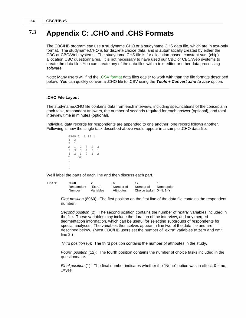
CBC/HB v564
7.3 Appendix C: .CHO and .CHS Formats
The CBC/HB program can use a studyname.CHO or a studyname.CHS data file, which are in text-onlyformat. The studyname.CHO is for discrete choice data, and is automatically created by either theCBC or CBC/Web systems. The studyname.CHS file is for allocation-based, constant sum (chip)allocation CBC questionnaires. It is not necessary to have used our CBC or CBC/Web systems tocreate the data file. You can create any of the data files with a text editor or other data processingsoftware.
Note: Many users will find the .CSV format data files easier to work with than the file formats describedbelow. You can quickly convert a .CHO file to .CSV using the Tools + Convert .cho to .csv option.
.CHO File Layout
The studyname.CHO file contains data from each interview, including specifications of the concepts ineach task, respondent answers, the number of seconds required for each answer (optional), and totalinterview time in minutes (optional).
Individual data records for respondents are appended to one another; one record follows another.Following is how the single task described above would appear in a sample .CHO data file:
8960 2 6 12 14 23 12 1 2 3 2 33 3 3 1 3 14 2 1 2 1 22 32...
We'll label the parts of each line and then discuss each part.
Line 1: 8960RespondentNumber
2"Extra"Variables
6Number ofAttributes
12Number ofChoice tasks
1None option0=N, 1=Y
First position (8960): The first position on the first line of the data file contains the respondentnumber.
Second position (2): The second position contains the number of "extra" variables included inthe file. These variables may include the duration of the interview, and any mergedsegmentation information, which can be useful for selecting subgroups of respondents forspecial analyses. The variables themselves appear in line two of the data file and aredescribed below. (Most CBC/HB users set the number of "extra" variables to zero and omitline 2.)
Third position (6): The third position contains the number of attributes in the study.
Fourth position (12): The fourth position contains the number of choice tasks included in thequestionnaire.
Final position (1): The final number indicates whether the "None" option was in effect; 0 = no,1=yes.
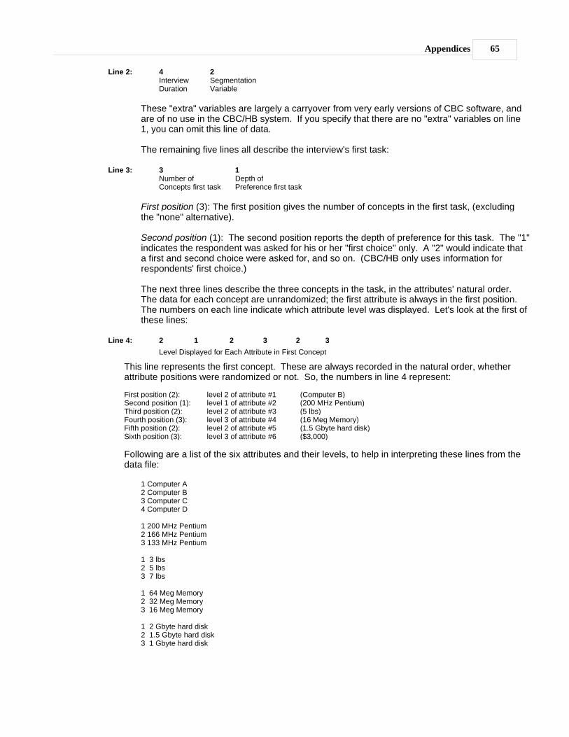
Appendices 65
Line 2: 4InterviewDuration
2SegmentationVariable
These "extra" variables are largely a carryover from very early versions of CBC software, andare of no use in the CBC/HB system. If you specify that there are no "extra" variables on line1, you can omit this line of data.
The remaining five lines all describe the interview's first task:
Line 3: 3Number ofConcepts first task
1Depth ofPreference first task
First position (3): The first position gives the number of concepts in the first task, (excludingthe "none" alternative).
Second position (1): The second position reports the depth of preference for this task. The "1"indicates the respondent was asked for his or her "first choice" only. A "2" would indicate thata first and second choice were asked for, and so on. (CBC/HB only uses information forrespondents' first choice.)
The next three lines describe the three concepts in the task, in the attributes' natural order.The data for each concept are unrandomized; the first attribute is always in the first position.The numbers on each line indicate which attribute level was displayed. Let's look at the first ofthese lines:
Line 4: 2 1 2 3 2 3
Level Displayed for Each Attribute in First Concept
This line represents the first concept. These are always recorded in the natural order, whetherattribute positions were randomized or not. So, the numbers in line 4 represent:
First position (2): level 2 of attribute #1 (Computer B)Second position (1): level 1 of attribute #2 (200 MHz Pentium)Third position (2): level 2 of attribute #3 (5 lbs)Fourth position (3): level 3 of attribute #4 (16 Meg Memory)Fifth position (2): level 2 of attribute #5 (1.5 Gbyte hard disk)Sixth position (3): level 3 of attribute #6 ($3,000)
Following are a list of the six attributes and their levels, to help in interpreting these lines from thedata file:
1 Computer A2 Computer B3 Computer C4 Computer D
1 200 MHz Pentium2 166 MHz Pentium3 133 MHz Pentium
1 3 lbs2 5 lbs3 7 lbs
1 64 Meg Memory2 32 Meg Memory3 16 Meg Memory
1 2 Gbyte hard disk2 1.5 Gbyte hard disk3 1 Gbyte hard disk

CBC/HB v566
1 $1,5002 $2,0003 $3,000
Line 5: 3 3 3 1 3 1
Level Displayed for Each Attribute in Second Concept
Line five represents the second concept, and the numbers are interpreted as:
First position (3): level 3 of attribute #1 (Computer C)Second position (3): level 3 of attribute #2 (133 MHz Pentium)Third position (3): level 3 of attribute #3 (7 lbs)Fourth position (1): level 1 of attribute #4 (64 Meg Memory)Fifth position (3): level 3 of attribute #5 (1 Gbyte hard disk)Sixth position (1): level 1 of attribute #6 ($1,500)
Line 6: 4 2 1 2 1 2
Level Displayed for Each Attribute in Third Concept
Line six represents the third concept, and the numbers are interpreted as:
First position (4): level 4 of attribute #1 (Computer D)Second position (2): level 2 of attribute #2 (166 MHz Pentium)Third position (1): level 1 of attribute #3 (3 lbs)Fourth position (2): level 2 of attribute #4 (32 Meg Memory)Fifth position (1): level 1 of attribute #5 (2 Gbyte hard disk)Sixth position (2): level 2 of attribute #6 ($2,000)
Line 7: 2Choice
32Task Duration
First position (2): The first position contains the respondent's choice, which in this example isconcept two.
Second position (32): The second position on this line contains the time it took, in seconds, for therespondent to give an answer to this task. This is optional information that doesn't affectcomputation, and any integer may be used if desired.
The balance of the respondent's data would consist of lines similar to the last five in our data filefragment, and those lines would have results for each of the other choice tasks.
.CHS File Layout
Following is a description of the .CHS format, for use with allocation-based (constant-sum) discretechoice experiments. (Please note that this format may also be used to code discrete choiceresponses, with the entire allocation given to the item chosen.) Individual data records for respondentsare appended to one another; one record follows another. Following is how the single task wouldappear in a sample .CHS data file:
8960 2 6 12 04 232 1 2 3 2 3 73 3 3 1 3 1 34 2 1 2 1 2 0...
We'll label the parts of each line and then discuss each part.
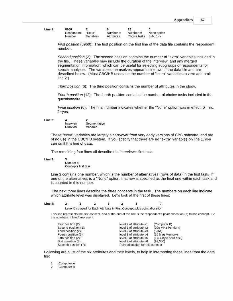
Appendices 67
Line 1: 8960RespondentNumber
2"Extra"Variables
6Number ofAttributes
12Number ofChoice tasks
0None option0=N, 1=Y
First position (8960): The first position on the first line of the data file contains the respondentnumber.
Second position (2): The second position contains the number of "extra" variables included inthe file. These variables may include the duration of the interview, and any mergedsegmentation information, which can be useful for selecting subgroups of respondents forspecial analyses. The variables themselves appear in line two of the data file and aredescribed below. (Most CBC/HB users set the number of "extra" variables to zero and omitline 2.)
Third position (6): The third position contains the number of attributes in the study.
Fourth position (12): The fourth position contains the number of choice tasks included in thequestionnaire.
Final position (0): The final number indicates whether the "None" option was in effect; 0 = no,1=yes.
Line 2: 4InterviewDuration
2SegmentationVariable
These "extra" variables are largely a carryover from very early versions of CBC software, and areof no use in the CBC/HB system. If you specify that there are no "extra" variables on line 1, youcan omit this line of data.
The remaining four lines all describe the interview's first task:
Line 3: 3Number ofConcepts first task
Line 3 contains one number, which is the number of alternatives (rows of data) in the first task. Ifone of the alternatives is a "None" option, that row is specified as the final one within each task andis counted in this number.
The next three lines describe the three concepts in the task. The numbers on each line indicatewhich attribute level was displayed. Let's look at the first of these lines:
Line 4: 2 1 2 3 2 3 7
Level Displayed for Each Attribute in First Concept, plus point allocation
This line represents the first concept, and at the end of the line is the respondent's point allocation (7) to this concept. Sothe numbers in line 4 represent:
First position (2): level 2 of attribute #1 (Computer B)Second position (1): level 1 of attribute #2 (200 MHz Pentium)Third position (2): level 2 of attribute #3 (5 lbs)Fourth position (3): level 3 of attribute #4 (16 Meg Memory)Fifth position (2): level 2 of attribute #5 (1.5 Gbyte hard disk)Sixth position (3): level 3 of attribute #6 ($3,000)Seventh position (7): Point allocation for this concept
Following are a list of the six attributes and their levels, to help in interpreting these lines from the datafile:
1 Computer A2 Computer B
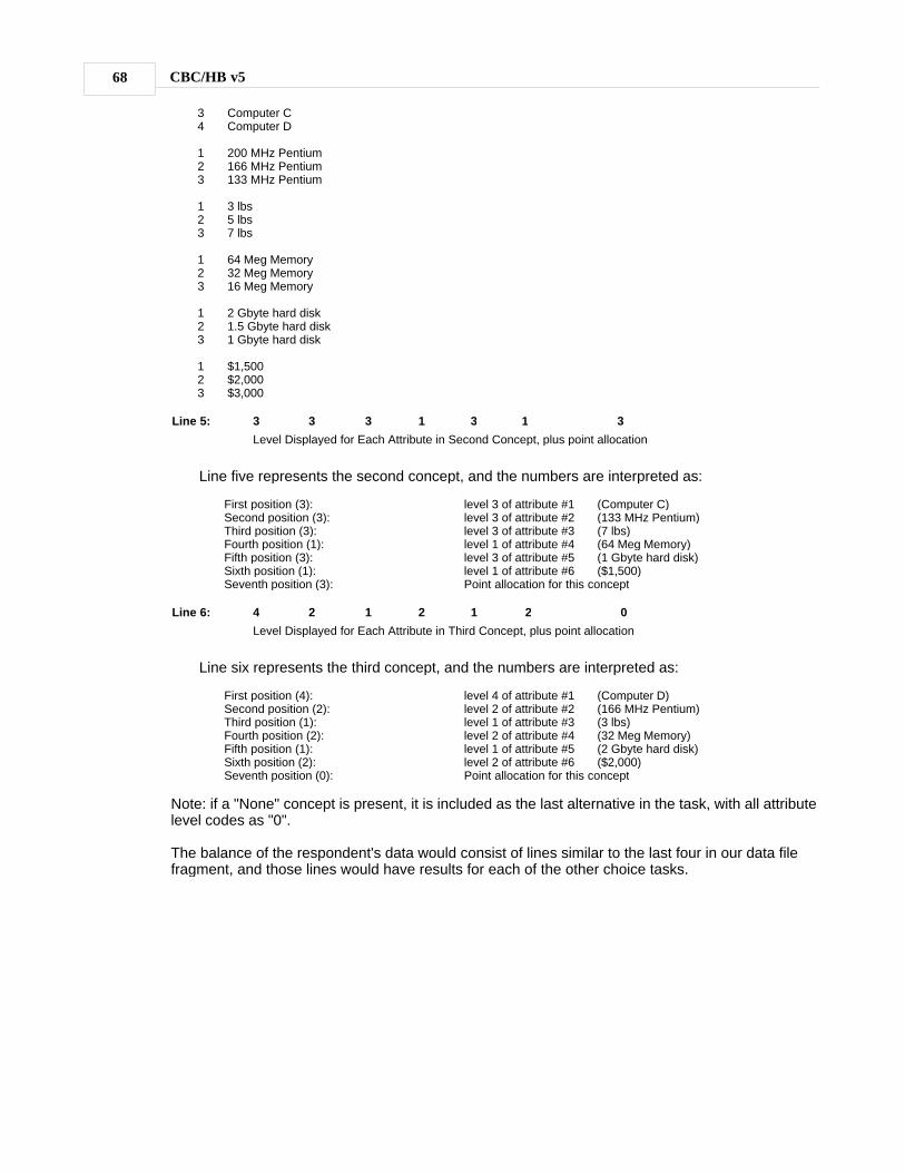
CBC/HB v568
3 Computer C4 Computer D
1 200 MHz Pentium2 166 MHz Pentium3 133 MHz Pentium
1 3 lbs2 5 lbs3 7 lbs
1 64 Meg Memory2 32 Meg Memory3 16 Meg Memory
1 2 Gbyte hard disk2 1.5 Gbyte hard disk3 1 Gbyte hard disk
1 $1,5002 $2,0003 $3,000
Line 5: 3 3 3 1 3 1 3
Level Displayed for Each Attribute in Second Concept, plus point allocation
Line five represents the second concept, and the numbers are interpreted as:
First position (3): level 3 of attribute #1 (Computer C)Second position (3): level 3 of attribute #2 (133 MHz Pentium)Third position (3): level 3 of attribute #3 (7 lbs)Fourth position (1): level 1 of attribute #4 (64 Meg Memory)Fifth position (3): level 3 of attribute #5 (1 Gbyte hard disk)Sixth position (1): level 1 of attribute #6 ($1,500)Seventh position (3): Point allocation for this concept
Line 6: 4 2 1 2 1 2 0
Level Displayed for Each Attribute in Third Concept, plus point allocation
Line six represents the third concept, and the numbers are interpreted as:
First position (4): level 4 of attribute #1 (Computer D)Second position (2): level 2 of attribute #2 (166 MHz Pentium)Third position (1): level 1 of attribute #3 (3 lbs)Fourth position (2): level 2 of attribute #4 (32 Meg Memory)Fifth position (1): level 1 of attribute #5 (2 Gbyte hard disk)Sixth position (2): level 2 of attribute #6 ($2,000)Seventh position (0): Point allocation for this concept
Note: if a "None" concept is present, it is included as the last alternative in the task, with all attributelevel codes as "0".
The balance of the respondent's data would consist of lines similar to the last four in our data filefragment, and those lines would have results for each of the other choice tasks.

Appendices 69
7.4
Appendix D: Directly Specifying Design Codes inthe .CHO or .CHS FilesSome advanced users of CBC/HB may want to control the coding of some or all of the independentvariables, rather than let CBC/HB automatically perform the effects coding based on the integers foundin the .CHO or .CHS files. When doing this, you set attribute coding to "User-specified" within theAttribute Information tab for any attribute for which you are controlling the coding.
When you specify that some attributes use "User-specified" coding, you are telling CBC/HB that certainor all values found in the .CHO or .CHS files should be used as-is within the design matrix (these mayalso be specified in the alternate .CSV data file formats, if you prefer to work with these). In theexample below, we'll let CBC/HB code automatically all but one of the parameters to be estimated.Even though we'll only show an example for a .CHO file, the same procedure is followed withinthe relevant format for the .CHS file.
Consider the following segment from a studyname.CHO file, representing the first of 18 tasks forrespondent number 2001 (if needed, please refer to Appendix C that describes the layout for thestudyname.CHO file):
2001 7 6 18 06 1 2 3 4 5 65 12 1 2 1 2 31 1 3 1 1 21 3 3 2 2 12 3 2 2 1 43 2 1 1 2 33 99
Attribute six in this example is Price (we've bolded the price codes for the five product conceptsavailable within this task). Price currently is coded as 4 levels. Let's imagine that the prices associatedwith these levels are:
Level 1 $10Level 2 $20Level 3 $30Level 4 $50
We should point out that CBC/HB operates better if the variances of the estimated parameters are nottoo different from the prior assumptions of unity, and the absolute magnitude of the parameters are notvastly different. Convergence occurs much more quickly and properly if this is the case. If there isenough information at the individual level, the priors should have little effect on the outcome. But, withCBC projects, the amount of information for each respondent is often sparse, and the scaling ofcolumns within the design matrix and resulting variance/scale of the estimated parameters maytherefore be important.
We recognize that the effects-coding procedure used for the categorical attributes results in columns inthe independent variable matrix coded as -1, 0, or +1. These codes are zero-centered, and have arange of 2 (+1 minus -1). Effects coding has worked well in practice with HB. We also suggest thatyou zero-center your variables and that they have a range not too different from effects coding.
In our example above, the prices are $10, $20, $30, $50. To zero-center the codes, we first subtractfrom each value the mean of the values. The mean is 27.5. Therefore, the zero-coded values are:
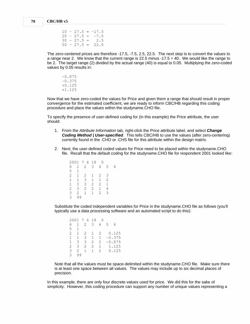
CBC/HB v570
10 - 27.5 = -17.520 - 27.5 = -7.530 - 27.5 = 2.550 - 27.5 = 22.5
The zero-centered prices are therefore -17.5, -7.5, 2.5, 22.5. The next step is to convert the values toa range near 2. We know that the current range is 22.5 minus -17.5 = 40. We would like the range tobe 2. The target range (2) divided by the actual range (40) is equal to 0.05. Multiplying the zero-codedvalues by 0.05 results in:
-0.875-0.375+0.125+1.125
Now that we have zero-coded the values for Price and given them a range that should result in properconvergence for the estimated coefficient, we are ready to inform CBC/HB regarding this codingprocedure and place the values within the studyname.CHO file.
To specify the presence of user-defined coding for (in this example) the Price attribute, the usershould:
1. From the Attribute Information tab, right-click the Price attribute label, and select ChangeCoding Method | User-specified. This tells CBC/HB to use the values (after zero-centering)currently found in the .CHO or .CHS file for this attribute within the design matrix.
2. Next, the user-defined coded values for Price need to be placed within the studyname.CHOfile. Recall that the default coding for the studyname.CHO file for respondent 2001 looked like:
2001 7 6 18 06 1 2 3 4 5 65 12 1 2 1 2 31 1 3 1 1 21 3 3 2 2 12 3 2 2 1 43 2 1 1 2 33 99
Substitute the coded independent variables for Price in the studyname.CHO file as follows (you'lltypically use a data processing software and an automated script to do this):
2001 7 6 18 06 1 2 3 4 5 65 12 1 2 1 2 0.1251 1 3 1 1 -0.3751 3 3 2 2 -0.8752 3 2 2 1 1.1253 2 1 1 2 0.1253 99
Note that all the values must be space-delimited within the studyname.CHO file. Make sure thereis at least one space between all values. The values may include up to six decimal places ofprecision.
In this example, there are only four discrete values used for price. We did this for the sake ofsimplicity. However, this coding procedure can support any number of unique values representing a

Appendices 71
continuous variable in the design matrix.

CBC/HB v572
7.5
Appendix E: Analyzing Alternative-Specific andPartial-Profile DesignsIntroduction
The CBC/HB System analyzes data from the studyname.CHO or studyname.CHS files, which are intext-only format. The studyname.CHO file is automatically generated by the CBC or CBC/Websystems, but you can create your own studyname.CHO or studyname.CHS files and analyze resultsfrom surveys that were designed and conducted in other ways.
Alternative-Specific Designs
Some researchers employ a specialized type of choice-based conjoint design wherein somealternatives (i.e. brands) have their own unique set of attributes. For example, consider different waysto get to work in the city: cars vs. buses. Each option has its own set of product features that areuniquely associated with that particular mode of transportation. These sorts of dependent attributeshave also been called "brand-specific attributes," though as our example illustrates, they aren't alwaystied to brands.
Consider the following design:
Car: Bus:
Gas: $1.25/ gallonGas: $1.50/ gallonGas: $1.75/ gallon
Picks up every 20 min.Picks up every 15 min.Picks up every 10 min.Picks up every 5 min.
Company-paid parkingParking lot: $5.00/dayParking lot: $7.00/day
25 cents per one-way trip50 cents per one-way trip75 cents per one-way trip$1.00 per one-way trip
Light traffic reportModerate traffic reportHeavy traffic report
There are actually six different attributes in this design:
1. Mode of transportation (2 levels: Car/Bus)2. Price of gas (3 levels)3. Car parking (3 levels)4. Traffic report (3 levels)5. Bus frequency (4 levels)6. Bus fare (4 levels)
Attributes two through four never appear with bus concepts, and attributes five and six never appearwith car concepts.
In the studyname.CHO and studyname.CHS files (described in detail in Appendix C), there is a row ofcoded values describing each product concept displayed in each task. Consider a two-alternative taskwith the following options:

Appendices 73
Car, Gas: $1.25/ gallon, Parking lot: $5.00/ day, Light traffic reportBus, Picks up every 10 min., 50 cents per one-way trip
Again, there are six total attributes used to describe two different modes of transportation. The twoalternatives above would be coded as follows in the studyname.cho or studyname.chs files:
1 1 2 1 0 02 0 0 0 3 2
Note that the attributes that do not apply to the current concept are coded as a 0 (zero).
Analyzing Partial-Profile Designs
Partial-profile designs display only a subset of the total number of attributes in each task. For example,there might be 12 total attributes in the design, but only five are displayed in any given task. As withcoding attribute-specific designs, we specify a level code of 0 (zero) for any attribute that is notapplicable (present) in the current product concept.
Analyzing More Than One Constant Alternative
Some discrete choice designs include more than one constant alternative. These alternatives aretypically defined using a single statement that never varies. With the transportation example above,other constant alternatives in the choice task might be: "I'd carpool with a co-worker" or "I'd walk towork." Multiple constant alternatives can be included in the design and analyzed with the CBC/HBSystem. If there is more than one constant alternative, one appropriate coding strategy is to representthese as additional levels of another attribute. For example, in the transportation example we've beenusing, rather than specifying just two levels for the first attribute (Car, Bus), we could specify fourcodes:
1 Car2 Bus3 I'd carpool with a co-worker4 I'd walk to work
You should specify four alternatives per task to accommodate the car, bus and the two constantalternatives. To code the task mentioned in the previous example plus two constant alternatives ineither the studyname.CHO or studyname.CHS files, you would specify:
1 1 2 1 0 02 0 0 0 3 23 0 0 0 0 04 0 0 0 0 0
It is worth noting that the advanced coding strategies outlined in this appendix are also useful withinCBC's standard logit, latent class and ICE systems. Though these systems cannot generate designsautomatically or questionnaires for these advanced designs, they can analyze choice data files codedto reflect them.

CBC/HB v574
7.6
Appendix F: How Constant Sum Data Are Treatedin CBC/HBIntroduction
Conjoint analysis has been an important marketing research technique for several decades. In recentyears, attention has focused on the analysis of choices, as opposed to rankings or ratings, giving riseto methodologies known as "Discrete Choice Analysis" or "Choice-Based Conjoint Analysis."
Choice analysis has the advantage that experimental choices can mimic actual buying situations moreclosely than other types of conjoint questions. However, choices also have a disadvantage:inefficiency in collecting data. A survey respondent must read and understand several productdescriptions before making an informed choice among them. Yet, after all of that cognitive processingthe respondent provides very scanty information, consisting of a single choice among alternatives.There is no information about intensity of preference, which products would be runners up, or whetherany other products would even be acceptable.
Many researchers favor the comparative nature of choice tasks, but are unwilling to settle for so littleinformation from each of them. This leads to the notion of asking respondents to answer more fully byallocating "constant sum scores" among the alternatives in each choice set rather than by just picking asingle one. For example, a survey respondent might be given 10 chips and asked to distribute themamong alternatives in each choice set according to his/her likelihood of purchasing each. Alternatively,the respondent might be asked to imagine the next 10 purchase occasions, and to estimate how manyunits of each alternative would be purchased in total on those occasions. Such information can beespecially informative in categories where the same individuals often choose a mix of products, suchas breakfast cereals or soft drinks. Constant sum scores are particularly appropriate when it isreasonable for the respondent to treat the units as probabilities or frequencies.
Constant sum scores certainly can provide more information than mere choices, although they are notwithout shortcomings of their own. One disadvantage is that it takes respondents longer to answerconstant sum tasks than choice tasks (Pinnell, 1999). Another is that one can't be sure of the mentalprocess a respondent uses in providing constant sum data. The requirement of summing to 10 orsome other total may get in the way of accurate reporting of relative strengths of preference. Finally,since respondents' processes of allocating points are unknown, it's not clear what assumptions shouldbe made in analyzing the resulting data.
The CBC/HB strategy for analyzing constant sum data begins with the notion that each constant sumpoint is the result of a separate choice among alternatives. Suppose 10 points are awarded amongthree alternatives, with the scores [7, 3, 0]. We could treat this as equivalent to 10 repeated choicetasks, in which the first alternative was chosen 7 times, the second chosen 3 times, and the third neverchosen. But, there is a difficulty with this approach: one can't be sure that constant sum points areequivalent to an aggregation of independent choices. Perhaps this respondent is inclined always togive about 7 points to his/her first choice and about 3 points to his/her second choice. Then we don'thave 10 independent choices, but something more like two.
Bayesian analysis provides superior results by combining data from each respondent with informationfrom others when estimating values for that respondent. These two sources of information arecombined in a way that reflects the relative strength of each. If a respondent conscientiously makes 10independent choices in allocating 10 points, then those data contain more information and shouldreceive greater weight than if he/she uses some simpler method. Likewise, if a respondent werealways to allocate points among products without really reflecting on the actual likelihood of choice,those data contain less information, and should be given less weight in estimation of his/her values.
With the CBC/HB module we deal with this problem by asking the analyst to estimate the amount of
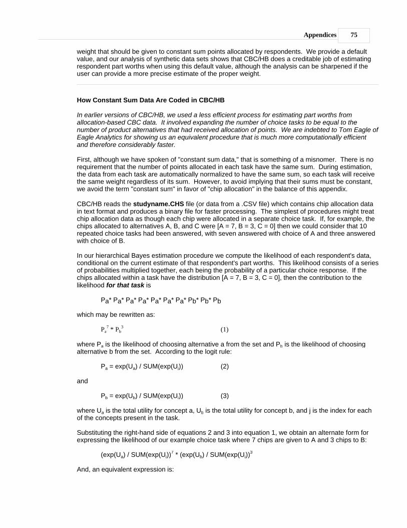
Appendices 75
weight that should be given to constant sum points allocated by respondents. We provide a defaultvalue, and our analysis of synthetic data sets shows that CBC/HB does a creditable job of estimatingrespondent part worths when using this default value, although the analysis can be sharpened if theuser can provide a more precise estimate of the proper weight.
How Constant Sum Data Are Coded in CBC/HB
In earlier versions of CBC/HB, we used a less efficient process for estimating part worths fromallocation-based CBC data. It involved expanding the number of choice tasks to be equal to thenumber of product alternatives that had received allocation of points. We are indebted to Tom Eagle ofEagle Analytics for showing us an equivalent procedure that is much more computationally efficientand therefore considerably faster.
First, although we have spoken of "constant sum data," that is something of a misnomer. There is norequirement that the number of points allocated in each task have the same sum. During estimation,the data from each task are automatically normalized to have the same sum, so each task will receivethe same weight regardless of its sum. However, to avoid implying that their sums must be constant,we avoid the term "constant sum" in favor of "chip allocation" in the balance of this appendix.
CBC/HB reads the studyname.CHS file (or data from a .CSV file) which contains chip allocation datain text format and produces a binary file for faster processing. The simplest of procedures might treatchip allocation data as though each chip were allocated in a separate choice task. If, for example, thechips allocated to alternatives A, B, and C were [A = 7, B = 3, C = 0] then we could consider that 10repeated choice tasks had been answered, with seven answered with choice of A and three answeredwith choice of B.
In our hierarchical Bayes estimation procedure we compute the likelihood of each respondent's data,conditional on the current estimate of that respondent's part worths. This likelihood consists of a seriesof probabilities multiplied together, each being the probability of a particular choice response. If thechips allocated within a task have the distribution [A = 7, B = 3, C = 0], then the contribution to thelikelihood for that task is
Pa* Pa* Pa* Pa* Pa* Pa* Pa* Pb* Pb* Pb
which may be rewritten as:
Pa7 * Pb
3 (1)
where Pa is the likelihood of choosing alternative a from the set and Pb is the likelihood of choosingalternative b from the set. According to the logit rule:
Pa = exp(Ua) / SUM(exp(Uj)) (2)
and
Pb = exp(Ub) / SUM(exp(Uj)) (3)
where Ua is the total utility for concept a, Ub is the total utility for concept b, and j is the index for eachof the concepts present in the task.
Substituting the right-hand side of equations 2 and 3 into equation 1, we obtain an alternate form forexpressing the likelihood of our example choice task where 7 chips are given to A and 3 chips to B:
(exp(Ua) / SUM(exp(Uj))7 * (exp(Ub) / SUM(exp(Uj))
3
And, an equivalent expression is:

CBC/HB v576
exp(Ua)7 * exp(Ub)
3 / SUM(exp(Uj))10 (4)
There is a potential problem when so many probabilities are multiplied together (equivalently, raisingthe probability of the alternative to the number of chips given to that alternative). The HB estimationalgorithm combines data from each respondent with data from others, and the relative weight given tothe respondent's own data is affected by the number of probabilities multiplied together. If therespondent really does answer by allocating each chip independently, then the likelihood should be theproduct of all those probabilities. But if the data were really generated by some simpler process, then ifwe multiply all those probabilities together, we will in effect be giving too much weight to therespondent's own data and too little to information from other respondents.
For this reason we give the user a parameter which we describe as "Total task weight." If the userbelieves that respondents allocated ten chips independently, he should use a value of ten. If hebelieves that the allocation of chips within a task are entirely dependent on one another (such as ifevery respondent awards all chips to the same alternative) he should use a value of one. Probably thetruth lies somewhere in between, and for that reason we suggest 5 as a default value.
We use the Task Weight in the following way.
Rather than assume that each chip represents an independent choice event, we first normalize thenumber of chips allocated within each task by dividing the exponents in equation 4 by the total numberof chips allocated. This simplifies the formula to:
exp(Ua)0.7 * exp(Ub)
0.3 / SUM(exp(Uj))
We can then apply the task weight to appropriately weight the task. Assuming the researcher wishesto apply a task weight of 5, the new formula to represent the probability of this task is:
[ exp(Ua)0.7 * exp(Ub)
0.3 / SUM(exp(Uj)) ]5
Which may be rewritten as:
exp(Ua)(0.7*5) * exp(Ub)
(0.3*5) / SUM(exp(Uj))5
Mathematically, this is identical to the likelihood expression based on expanded tasks that we used inearlier versions of CBC/HB software, but it avoids expanding the tasks and is more efficientcomputationally.
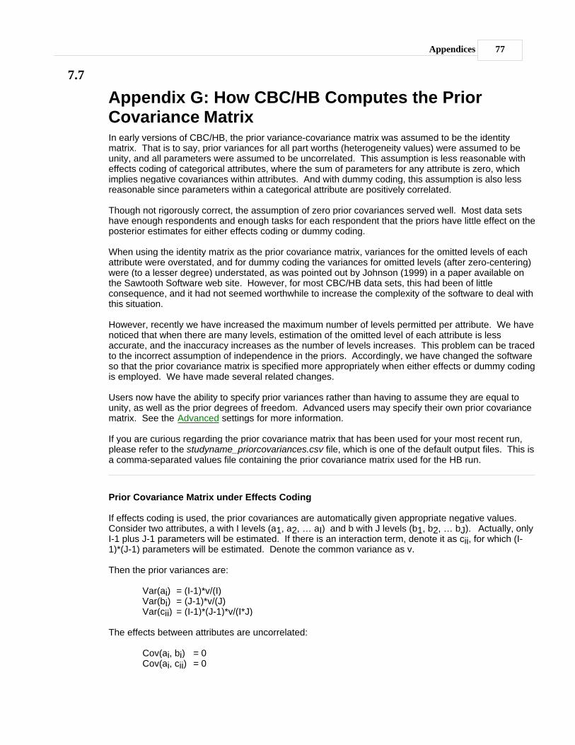
Appendices 77
7.7
Appendix G: How CBC/HB Computes the PriorCovariance MatrixIn early versions of CBC/HB, the prior variance-covariance matrix was assumed to be the identitymatrix. That is to say, prior variances for all part worths (heterogeneity values) were assumed to beunity, and all parameters were assumed to be uncorrelated. This assumption is less reasonable witheffects coding of categorical attributes, where the sum of parameters for any attribute is zero, whichimplies negative covariances within attributes. And with dummy coding, this assumption is also lessreasonable since parameters within a categorical attribute are positively correlated.
Though not rigorously correct, the assumption of zero prior covariances served well. Most data setshave enough respondents and enough tasks for each respondent that the priors have little effect on theposterior estimates for either effects coding or dummy coding.
When using the identity matrix as the prior covariance matrix, variances for the omitted levels of eachattribute were overstated, and for dummy coding the variances for omitted levels (after zero-centering)were (to a lesser degree) understated, as was pointed out by Johnson (1999) in a paper available onthe Sawtooth Software web site. However, for most CBC/HB data sets, this had been of littleconsequence, and it had not seemed worthwhile to increase the complexity of the software to deal withthis situation.
However, recently we have increased the maximum number of levels permitted per attribute. We havenoticed that when there are many levels, estimation of the omitted level of each attribute is lessaccurate, and the inaccuracy increases as the number of levels increases. This problem can be tracedto the incorrect assumption of independence in the priors. Accordingly, we have changed the softwareso that the prior covariance matrix is specified more appropriately when either effects or dummy codingis employed. We have made several related changes.
Users now have the ability to specify prior variances rather than having to assume they are equal tounity, as well as the prior degrees of freedom. Advanced users may specify their own prior covariancematrix. See the Advanced settings for more information.
If you are curious regarding the prior covariance matrix that has been used for your most recent run,please refer to the studyname_priorcovariances.csv file, which is one of the default output files. This isa comma-separated values file containing the prior covariance matrix used for the HB run.
Prior Covariance Matrix under Effects Coding
If effects coding is used, the prior covariances are automatically given appropriate negative values.Consider two attributes, a with I levels (a1, a2, … aI) and b with J levels (b1, b2, … bJ). Actually, onlyI-1 plus J-1 parameters will be estimated. If there is an interaction term, denote it as cij, for which (I-1)*(J-1) parameters will be estimated. Denote the common variance as v.
Then the prior variances are:
Var(ai) = (I-1)*v/(I)Var(bj) = (J-1)*v/(J)Var(cij) = (I-1)*(J-1)*v/(I*J)
The effects between attributes are uncorrelated:
Cov(ai, bj) = 0Cov(ai, cij) = 0
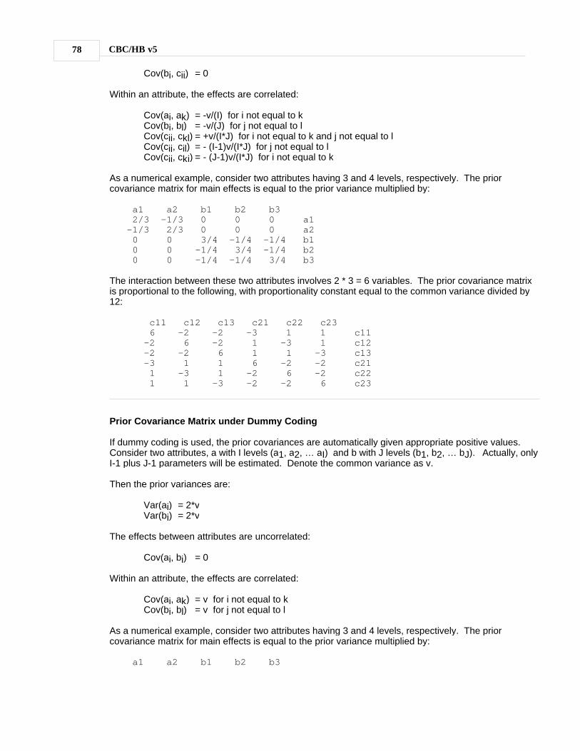
CBC/HB v578
Cov(bj, cij) = 0 Within an attribute, the effects are correlated:
Cov(ai, ak) = -v/(I) for i not equal to kCov(bj, bl) = -v/(J) for j not equal to l Cov(cij, ckl) = +v/(I*J) for i not equal to k and j not equal to lCov(cij, cil) = - (I-1)v/(I*J) for j not equal to lCov(cij, ckj) = - (J-1)v/(I*J) for i not equal to k
As a numerical example, consider two attributes having 3 and 4 levels, respectively. The priorcovariance matrix for main effects is equal to the prior variance multiplied by:
a1 a2 b1 b2 b3 2/3 -1/3 0 0 0 a1 -1/3 2/3 0 0 0 a2 0 0 3/4 -1/4 -1/4 b1 0 0 -1/4 3/4 -1/4 b2 0 0 -1/4 -1/4 3/4 b3
The interaction between these two attributes involves 2 * 3 = 6 variables. The prior covariance matrixis proportional to the following, with proportionality constant equal to the common variance divided by12:
c11 c12 c13 c21 c22 c23 6 -2 -2 -3 1 1 c11-2 6 -2 1 -3 1 c12-2 -2 6 1 1 -3 c13-3 1 1 6 -2 -2 c21 1 -3 1 -2 6 -2 c22 1 1 -3 -2 -2 6 c23
Prior Covariance Matrix under Dummy Coding
If dummy coding is used, the prior covariances are automatically given appropriate positive values.Consider two attributes, a with I levels (a1, a2, … aI) and b with J levels (b1, b2, … bJ). Actually, onlyI-1 plus J-1 parameters will be estimated. Denote the common variance as v.
Then the prior variances are:
Var(ai) = 2*vVar(bj) = 2*v
The effects between attributes are uncorrelated:
Cov(ai, bj) = 0
Within an attribute, the effects are correlated:
Cov(ai, ak) = v for i not equal to kCov(bj, bl) = v for j not equal to l
As a numerical example, consider two attributes having 3 and 4 levels, respectively. The priorcovariance matrix for main effects is equal to the prior variance multiplied by:
a1 a2 b1 b2 b3
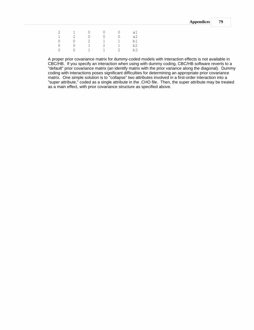
Appendices 79
2 1 0 0 0 a1 1 2 0 0 0 a2 0 0 2 1 1 b1 0 0 1 2 1 b2 0 0 1 1 2 b3
A proper prior covariance matrix for dummy-coded models with interaction effects is not available inCBC/HB. If you specify an interaction when using with dummy coding, CBC/HB software reverts to a"default" prior covariance matrix (an identify matrix with the prior variance along the diagonal). Dummycoding with interactions poses significant difficulties for determining an appropriate prior covariancematrix. One simple solution is to "collapse" two attributes involved in a first-order interaction into a"super attribute," coded as a single attribute in the .CHO file. Then, the super attribute may be treatedas a main effect, with prior covariance structure as specified above.

CBC/HB v580
7.8 Appendix H: Generating a .CHS File
The .CHS file format is used when respondents have used constant sum (chip allocation) foranswering CBC questions. Its format is provided in Appendix C. Until allocation-based CBCquestionnaires are directly supported within the SMRT or SSI Web platforms, some users may find atool provided in CBC/HB convenient for generating .CHS files.
Clicking Tools | Convert CHO to CHS… accesses a tool that takes data provided in a .CHO formatand converts it to a .CHS format. Optionally, the user can supply a separate text-only file ofrespondent answers (delimited by spaces, tabs, or hard returns). CBC/HB combines the allocationinformation found in the file of respondent answers with the information provided in the .CHO file,creating a .CHS file. Any choice responses found in the .CHO file are overwritten by allocationresponses found in the optional file of respondent answers.
For example, the first two lines (representing the first two respondents) in the text-only file containingrespondent answers may look like:
1001 50 0 50 80 20 0 100 0 0 ... (more data follow)1002 100 0 0 90 0 10 80 20 0 ... (more data follow)
This file must begin with the respondent number. The respondent records do not need to be in thesame order as in the .CHO file and the two files do not need to have the same number of cases. If arespondent's allocation data are not provided but that respondent exists in the .CHO file, originalanswers in the .CHO file for this respondent are written to the .CHS file.
In this example, three concepts were shown per choice task. Therefore, the first three values(representing task #1) sum to 100, the next three values (representing task #2) sum to 100, etc. It isnot necessary that the values within a task sum to 100 (but the total points allocated within a taskshould not exceed 100). If respondents skipped a task, you should allocate 0 points to all conceptswithin that task.
Example:
1. With CBC for Windows or CBC/Web, the user creates a paper-and-pencil questionnaire andfields the study.
2. Using a text-only file containing respondent numbers, questionnaire versions, and "dummy"choice responses, the user utilizes the automatic Accumulate Paper & Pencil Data functionand the File | Export functionality to export the data to a .CHO file.
3. The user provides a text-only file of respondent answers to the allocation questions (asdescribed above).
4. Using the Tools | Convert CHO to CHS… functionality in CBC/HB, the user merges theinformation from the .CHO file and the file of respondent answers to create a final .CHS file.
5. CBC/HB estimates part worths using the final .CHS file.
Future versions of our CBC software may automatically collect allocation-based responses andgenerate a .CHS file, which will eliminate the extra steps involved.
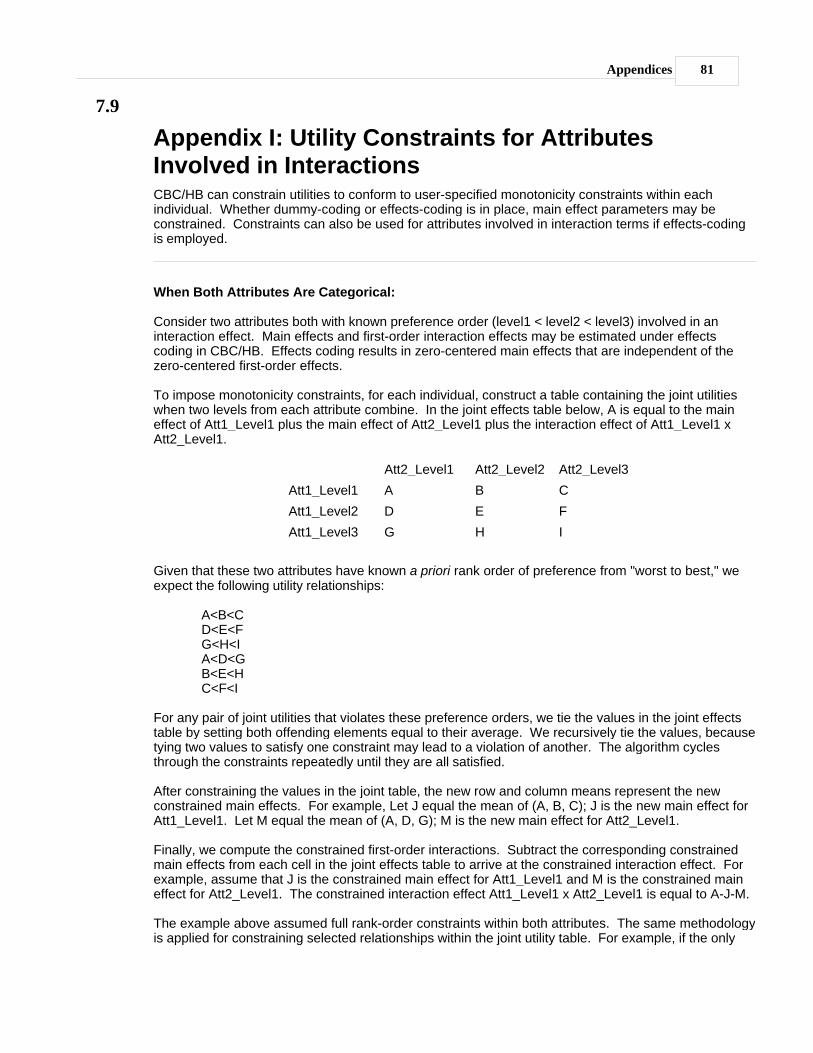
Appendices 81
7.9
Appendix I: Utility Constraints for AttributesInvolved in InteractionsCBC/HB can constrain utilities to conform to user-specified monotonicity constraints within eachindividual. Whether dummy-coding or effects-coding is in place, main effect parameters may beconstrained. Constraints can also be used for attributes involved in interaction terms if effects-codingis employed.
When Both Attributes Are Categorical:
Consider two attributes both with known preference order (level1 < level2 < level3) involved in aninteraction effect. Main effects and first-order interaction effects may be estimated under effectscoding in CBC/HB. Effects coding results in zero-centered main effects that are independent of thezero-centered first-order effects.
To impose monotonicity constraints, for each individual, construct a table containing the joint utilitieswhen two levels from each attribute combine. In the joint effects table below, A is equal to the maineffect of Att1_Level1 plus the main effect of Att2_Level1 plus the interaction effect of Att1_Level1 xAtt2_Level1.
Att2_Level1 Att2_Level2 Att2_Level3
Att1_Level1 A B C
Att1_Level2 D E F
Att1_Level3 G H I
Given that these two attributes have known a priori rank order of preference from "worst to best," weexpect the following utility relationships:
A<B<CD<E<FG<H<IA<D<GB<E<HC<F<I
For any pair of joint utilities that violates these preference orders, we tie the values in the joint effectstable by setting both offending elements equal to their average. We recursively tie the values, becausetying two values to satisfy one constraint may lead to a violation of another. The algorithm cyclesthrough the constraints repeatedly until they are all satisfied.
After constraining the values in the joint table, the new row and column means represent the newconstrained main effects. For example, Let J equal the mean of (A, B, C); J is the new main effect forAtt1_Level1. Let M equal the mean of (A, D, G); M is the new main effect for Att2_Level1.
Finally, we compute the constrained first-order interactions. Subtract the corresponding constrainedmain effects from each cell in the joint effects table to arrive at the constrained interaction effect. Forexample, assume that J is the constrained main effect for Att1_Level1 and M is the constrained maineffect for Att2_Level1. The constrained interaction effect Att1_Level1 x Att2_Level1 is equal to A-J-M.
The example above assumed full rank-order constraints within both attributes. The same methodologyis applied for constraining selected relationships within the joint utility table. For example, if the only
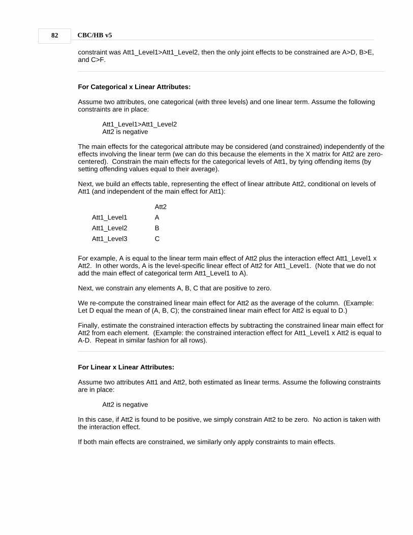
CBC/HB v582
constraint was Att1_Level1>Att1_Level2, then the only joint effects to be constrained are A>D, B>E,and C>F.
For Categorical x Linear Attributes:
Assume two attributes, one categorical (with three levels) and one linear term. Assume the followingconstraints are in place:
Att1_Level1>Att1_Level2Att2 is negative
The main effects for the categorical attribute may be considered (and constrained) independently of theeffects involving the linear term (we can do this because the elements in the X matrix for Att2 are zero-centered). Constrain the main effects for the categorical levels of Att1, by tying offending items (bysetting offending values equal to their average).
Next, we build an effects table, representing the effect of linear attribute Att2, conditional on levels ofAtt1 (and independent of the main effect for Att1):
Att2
Att1_Level1 A
Att1_Level2 B
Att1_Level3 C
For example, A is equal to the linear term main effect of Att2 plus the interaction effect Att1_Level1 xAtt2. In other words, A is the level-specific linear effect of Att2 for Att1_Level1. (Note that we do notadd the main effect of categorical term Att1_Level1 to A).
Next, we constrain any elements A, B, C that are positive to zero.
We re-compute the constrained linear main effect for Att2 as the average of the column. (Example:Let D equal the mean of (A, B, C); the constrained linear main effect for Att2 is equal to D.)
Finally, estimate the constrained interaction effects by subtracting the constrained linear main effect forAtt2 from each element. (Example: the constrained interaction effect for Att1_Level1 x Att2 is equal toA-D. Repeat in similar fashion for all rows).
For Linear x Linear Attributes:
Assume two attributes Att1 and Att2, both estimated as linear terms. Assume the following constraintsare in place:
Att2 is negative
In this case, if Att2 is found to be positive, we simply constrain Att2 to be zero. No action is taken withthe interaction effect.
If both main effects are constrained, we similarly only apply constraints to main effects.
Appendices 83
7.10 Appendix J: Estimation for Dual-Response "None"
Introduction
Some researchers have advocated asking the "None" choice as a second-stage question in discretechoice questionnaires (see "Beyond the Basics: Choice Modelling Methods and ImplementationIssues" (Brazell, Diener, Severin, and Uldry) in ART Tutorial 2003, American Marketing Association).The "Dual-Response None" technique is an application of the "buy/no buy" response that previousresearchers (including McFadden, Louviere, and Eagle) have used as an extension of standarddiscrete choice tasks since at least the early 1990s, and have modeled with nested logit.
The "Dual-Response None" approach is as follows. Rather than ask respondents to choose among,say, four alternatives {A, B, C and None}; respondents are first asked to choose among alternatives {A,B, and C}, and then next asked if they really would buy the alternative they selected in the first stage(yes/no).
The dual-response None dramatically increases the propensity of respondents to say "None," whichmany researchers would argue better reflects actual purchase intentions than when the "None" isasked in the standard way. But, no information is lost due to the selection of the "None," sincerespondents are first asked to discriminate among available products. Thus, the "Dual-Response"none can provide a "safety net": we can estimate a "None" parameter without worrying about thepotential decrease in precision of the other parameters if the incidence of "None" usage is quite high.
The "Dual-Response None" has its drawbacks. It adds a little bit more time to each choice task, sincerespondents must provide two answers rather than one. But, the additional time requirement isminimal, since respondents have already invested the time to become familiar with the alternatives inthe choice task. It is also possible that asking the "None" as a separate question may bias theparameters of interest.
Brazell et al. have suggested that the benefits of the dual response seem to outweigh any negatives.They have conducted split-sample experiments with respondents that demonstrate that the parameters(other than the "None") are not significantly different when using the standard "None" vs. "Dual-Response None" formats.
Modeling Dual-Response None in CBC/HB
We do not claim to know the absolute best method for modeling choice tasks that use the "Dual-Response None." However, the method we offer in CBC/HB seems to work quite well based on recenttests with actual respondent data and holdout choice tasks.
Our approach is quite simple: we model the two choices (the forced choice among alternatives, andthe buy/no buy follow-up) as independent choice tasks. In the first task, the choice is among availableproducts (without a "None" alternative available). In the second task, the choice is among availableproducts and the "None" alternative. Failure to pick the "None" alternative in the second stage (a "buy"indication) results in a redundant task. All information may be represented using just the second stagechoice task. With that one task, we can indicate the available options, which option the respondentchose, and the fact that the respondent rejected the "None" alternative. Therefore, we omit theredundant first-stage task.
Data Setup in the CBC/HB File
We already introduced the .CHO file layout in Appendix C. When using "Dual-Response None"questionnaires, make the following modifications:
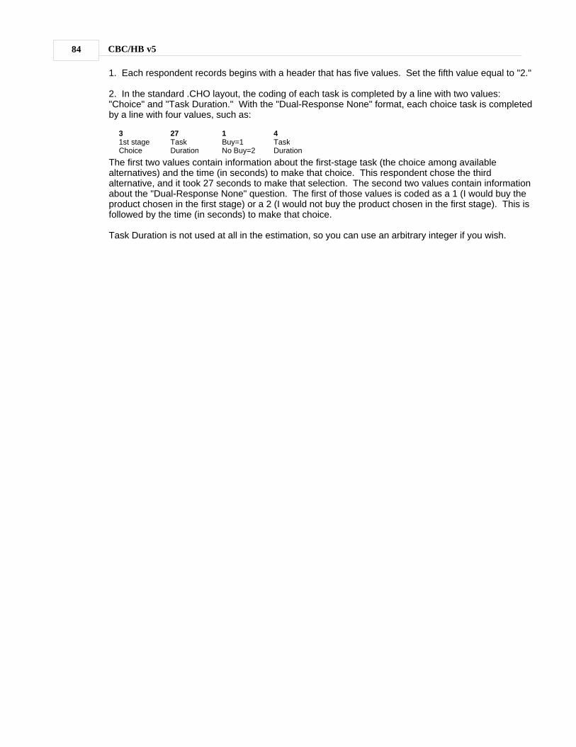
CBC/HB v584
1. Each respondent records begins with a header that has five values. Set the fifth value equal to "2."
2. In the standard .CHO layout, the coding of each task is completed by a line with two values:"Choice" and "Task Duration." With the "Dual-Response None" format, each choice task is completedby a line with four values, such as:
31st stageChoice
27TaskDuration
1Buy=1No Buy=2
4TaskDuration
The first two values contain information about the first-stage task (the choice among availablealternatives) and the time (in seconds) to make that choice. This respondent chose the thirdalternative, and it took 27 seconds to make that selection. The second two values contain informationabout the "Dual-Response None" question. The first of those values is coded as a 1 (I would buy theproduct chosen in the first stage) or a 2 (I would not buy the product chosen in the first stage). This isfollowed by the time (in seconds) to make that choice.
Task Duration is not used at all in the estimation, so you can use an arbitrary integer if you wish.
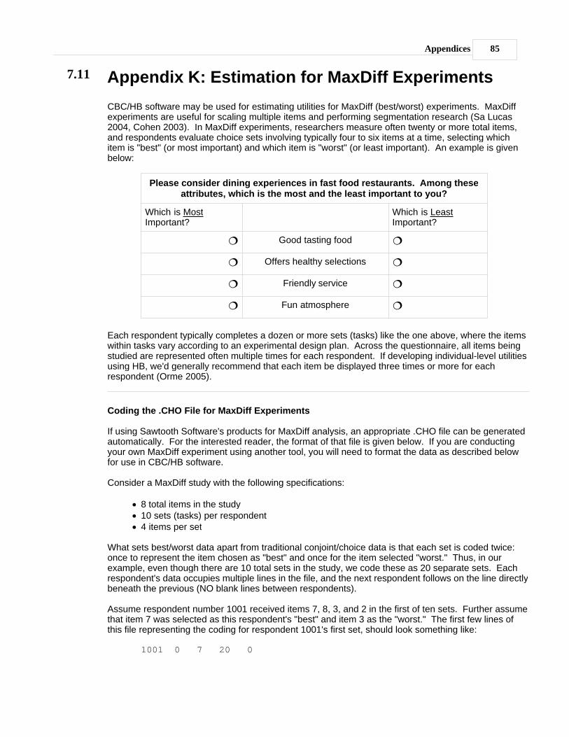
Appendices 85
7.11 Appendix K: Estimation for MaxDiff Experiments
CBC/HB software may be used for estimating utilities for MaxDiff (best/worst) experiments. MaxDiffexperiments are useful for scaling multiple items and performing segmentation research (Sa Lucas2004, Cohen 2003). In MaxDiff experiments, researchers measure often twenty or more total items,and respondents evaluate choice sets involving typically four to six items at a time, selecting whichitem is "best" (or most important) and which item is "worst" (or least important). An example is givenbelow:
Please consider dining experiences in fast food restaurants. Among theseattributes, which is the most and the least important to you?
Which is MostImportant?
Which is LeastImportant?
¦ Good tasting food ¦
¦ Offers healthy selections ¦
¦ Friendly service ¦
¦ Fun atmosphere ¦
Each respondent typically completes a dozen or more sets (tasks) like the one above, where the itemswithin tasks vary according to an experimental design plan. Across the questionnaire, all items beingstudied are represented often multiple times for each respondent. If developing individual-level utilitiesusing HB, we'd generally recommend that each item be displayed three times or more for eachrespondent (Orme 2005).
Coding the .CHO File for MaxDiff Experiments
If using Sawtooth Software's products for MaxDiff analysis, an appropriate .CHO file can be generatedautomatically. For the interested reader, the format of that file is given below. If you are conductingyour own MaxDiff experiment using another tool, you will need to format the data as described belowfor use in CBC/HB software.
Consider a MaxDiff study with the following specifications:
· 8 total items in the study· 10 sets (tasks) per respondent· 4 items per set
What sets best/worst data apart from traditional conjoint/choice data is that each set is coded twice:once to represent the item chosen as "best" and once for the item selected "worst." Thus, in ourexample, even though there are 10 total sets in the study, we code these as 20 separate sets. Eachrespondent's data occupies multiple lines in the file, and the next respondent follows on the line directlybeneath the previous (NO blank lines between respondents).
Assume respondent number 1001 received items 7, 8, 3, and 2 in the first of ten sets. Further assumethat item 7 was selected as this respondent's "best" and item 3 as the "worst." The first few lines ofthis file representing the coding for respondent 1001's first set, should look something like:
1001 0 7 20 0
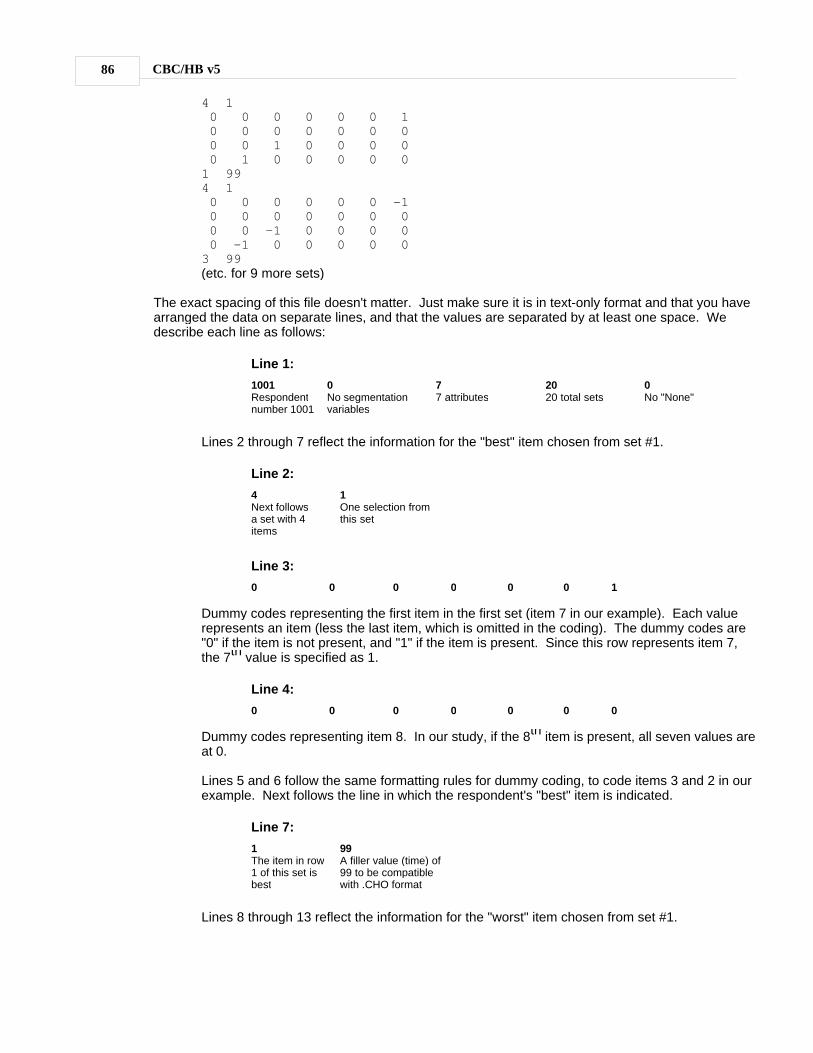
CBC/HB v586
4 1 0 0 0 0 0 0 1 0 0 0 0 0 0 0 0 0 1 0 0 0 0 0 1 0 0 0 0 01 994 1 0 0 0 0 0 0 -1 0 0 0 0 0 0 0 0 0 -1 0 0 0 0 0 -1 0 0 0 0 03 99(etc. for 9 more sets)
The exact spacing of this file doesn't matter. Just make sure it is in text-only format and that you havearranged the data on separate lines, and that the values are separated by at least one space. Wedescribe each line as follows:
Line 1:
1001Respondentnumber 1001
0No segmentationvariables
77 attributes
2020 total sets
0No "None"
Lines 2 through 7 reflect the information for the "best" item chosen from set #1.
Line 2:
4Next followsa set with 4items
1One selection fromthis set
Line 3:
0 0 0 0 0 0 1
Dummy codes representing the first item in the first set (item 7 in our example). Each valuerepresents an item (less the last item, which is omitted in the coding). The dummy codes are"0" if the item is not present, and "1" if the item is present. Since this row represents item 7,the 7th value is specified as 1.
Line 4:
0 0 0 0 0 0 0
Dummy codes representing item 8. In our study, if the 8th item is present, all seven values areat 0.
Lines 5 and 6 follow the same formatting rules for dummy coding, to code items 3 and 2 in ourexample. Next follows the line in which the respondent's "best" item is indicated.
Line 7:
1The item in row1 of this set isbest
99A filler value (time) of99 to be compatiblewith .CHO format
Lines 8 through 13 reflect the information for the "worst" item chosen from set #1.

Appendices 87
Line 8:
4Here followsa set with 4items
1One selection fromthis set
Lines 9 through 12 reflect the dummy codes (inverted) for the items shown in set one,considered with respect to the "worst" item selected. All values that were "1" in the previoustask are now "-1".
Line 13:
3The item in row3 of this set isbest
99A filler value (time) of99 to be compatiblewith .CHO format
Estimating the Model using CBC/HB
From the Choice Data File tab, browse to the .CHO file. On the Attribute Information tab, modify allattributes to have "User-specified coding." (Note that there will be k-1 total attributes in the study,representing your k total items in the MaxDiff design.)
We should note that when using HB to estimate parameters for many items under dummy coding, theestimates of the parameters (relative to the reference "0" level) can sometimes be distorted downward,often quite severely when there are many items in the study and when the number of questions askedof any one respondent is relatively few. (This distortion of course makes it appear as if the "omitted"item's estimate is "too high" relative to the others.) To see if this difficulty is appearing for your dataset, you might try coding a different level as the "omitted" item and compare the results. Or, you couldtake the step described below to avoid the problem.
To avoid potential problems when dealing with dummy coding under HB and very sparse dataconditions, you should specify a more appropriate "custom prior covariance matrix" from the AdvancedEstimation Settings tab. Check the custom prior covariance matrix box and click Edit.... Specify a (k-1) x (k-1) matrix of values, where k is equal to the total items in your MaxDiff study, a k-1 is equal tothe total number of parameters to be estimated (also equal to the number of attributes in the AttributeInformation tab). If you wish to specify a prior variance of 1.0 (a typical default), the matrix iscomposed of "2"s across the main diagonal, and "1"s in the off-diagonal positions, such as:
2 1 1 1 . . .1 2 1 1 . . .1 1 2 1 . . .1 1 1 2 . . .. . . . . . .. . . . . . .. . . . . . .
To specify a different prior variance, multiply all values in the prior covariance matrix above by thedesired variance constant.
When you have finished these steps, click Estimate Parameters Now... from the Home tab. Utilityvalues are written to the .HBU and .CSV files. Remember, the utility of the omitted value for eachrespondent is 0, and the other items are measured with respect to that omitted item.
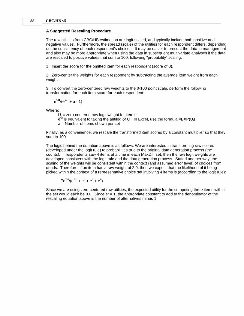
CBC/HB v588
A Suggested Rescaling Procedure
The raw utilities from CBC/HB estimation are logit-scaled, and typically include both positive andnegative values. Furthermore, the spread (scale) of the utilities for each respondent differs, dependingon the consistency of each respondent's choices. It may be easier to present the data to managementand also may be more appropriate when using the data in subsequent multivariate analyses if the dataare rescaled to positive values that sum to 100, following "probability" scaling.
1. Insert the score for the omitted item for each respondent (score of 0).
2. Zero-center the weights for each respondent by subtracting the average item weight from eachweight.
3. To convert the zero-centered raw weights to the 0-100 point scale, perform the followingtransformation for each item score for each respondent:
eUi/(eUi + a - 1)
Where:Ui = zero-centered raw logit weight for item ieUi is equivalent to taking the antilog of Ui. In Excel, use the formula =EXP(Ui)a = Number of items shown per set
Finally, as a convenience, we rescale the transformed item scores by a constant multiplier so that theysum to 100.
The logic behind the equation above is as follows: We are interested in transforming raw scores(developed under the logit rule) to probabilities true to the original data generation process (thecounts). If respondents saw 4 items at a time in each MaxDiff set, then the raw logit weights aredeveloped consistent with the logit rule and the data generation process. Stated another way, thescaling of the weights will be consistent within the context (and assumed error level) of choices fromquads. Therefore, if an item has a raw weight of 2.0, then we expect that the likelihood of it beingpicked within the context of a representative choice set involving 4 items is (according to the logit rule):
Ee2.0/(e2.0 + e0 + e0 + e0)
Since we are using zero-centered raw utilities, the expected utility for the competing three items withinthe set would each be 0.0. Since e0 = 1, the appropriate constant to add to the denominator of therescaling equation above is the number of alternatives minus 1.

Appendices 89
7.12 Appendix L: Hardware Recommendations
The CBC/HB System requires a fast computer and a generous amount of storage space, as offered bymost every PC that can be purchased today. By today's standards, a PC with a 2.8 GHz processor, 2GB RAM, and 200 GB of storage space is very adequate to run CBC/HB for most problems.
Many people equate processor speed with overall speed. This is not the only factor. Overall speed isdetermined by the combination of processor speed, storage space speed/availability, and memoryavailability. The fastest processors on the market will not make the system significantly faster if thestorage space and memory are too low. This is especially true for CBC/HB. While the algorithm iscomputationally intensive, it is often 'I/O bound' which means the running time is more dependent onfactors such as storage space and memory. The data files in use by CBC/HB are either located on thehard drive or in memory, and are referenced quite often. If these are slow, or their capacities areinsufficient, the fastest processor on the market will still appear to be slow.
In general, hard drive performance is optimal when the total used space is less than 50% of thecapacity of the drive. Keep this in mind when selecting a hard drive. Other factors that affectperformance are: transfer rate, seek time, and the drive's RPM (revolutions per minute) speed.
Memory is often overlooked as a speed-increasing factor. When operating systems such as Windowsbegin to run out of memory, they swap things on and off the hard drive (called thrashing). This canbring a system to a standstill. Again, the rule of thumb is to have about twice as much memory astypically used. Various utilities can diagnose how much memory is commonly used. If the systemtakes a long time to start up, or if you notice that the hard drive activity light is on almost constantly,these are signs of insufficient memory.
Other common hardware questions:
Is there a 64-bit version of CBC/HB? Would I benefit from a 64-bit system?
CBC/HB v5 runs in 64-bit mode when using 64-bit versions of Windows, and in 32-bit mode on 32-bitWindows. Our tests of 64-bit performance can be found in the Winter 2008 Sawtooth Solutions ("X64HB: Making Fast Even Faster"), available at Sawtooth Software's website. In those tests, we foundperformance increases typically between 10%-25%.
Can CBC/HB use multi-core processors? Would such a system be faster?
Today most new machines contain multi-core processors, which allow multiple tasks to be performedsimultaneously. For a program to take advantage of multiple processors it must be "multi-threaded,"which means that the software must run independent tasks on separate "threads." The key is thateach thread must be independent (i.e. rendering each pixel of an image can be done separately).While there are portions of the CBC/HB algorithm that are computed independently, overall thealgorithm is highly dependent and thus does not lend itself well to multi-threading. We continue to doresearch in this area.
However, CBC/HB does benefit indirectly from having multiple processors. When faced with a processdoing an intense computation, the operating system will attempt to give the process its own processor,and shift other processes to the other processors. So, if CBC/HB can run on one processor whileeverything else runs on others, it will run faster than when it must share only one processor.
CBC/HB v590
7.13
Appendix M: Calibrating Part-Worths for PurchaseLikelihoodIf you have asked additional Calibration Concept questions and formatted the calibration data in anappropriate format (see layout below), you can calibrate the part worth utilities for use with SawtoothSoftware's purchase likelihood simulation model within the market simulator. To calibrate the data,select Tools | Calibrate Utilities.... When you calibrate utilities, a new file is written namedstudyname_calib.hbu.
Background
In the mid-1990s, before computers were fast enough to make HB estimation feasible in marketresearch applications for medium to large CBC datasets, Sawtooth Software developed a fastprocedure for individual-level part worth estimation called ICE (Individual Choice Estimation). As partof the ICE procedure, we provided a way for users to display a Calibration Concept section (similar tothat offered by the earlier ACA system), and to use results from that section to calibrate (rescale) theutilities for use within Sawtooth Software's Purchase Likelihood Simulation Model.
Calibration Concept sections involve showing respondents multiple product concepts (in full-profile)one-at-a-time and asking them to rate their purchase likelihood (typically on a 100-point scale) for eachconcept.
Calibrated utilities are scaled such that when the sums of product utilities are submitted to the followingequation, they produce a least-squares fit to respondents' stated purchase likelihood on a 100-pointscale:
Purchase Likelihood = 100 * [ eUi / (1 + eUi) ]
where Ui is the total utility for the product concept and e is the exponential constant.
The Regression Equation
To calibrate the part worth utilities to fit purchase likelihood, we fit an ordinary least squares regression(for each respondent) relating part worth utilities to purchase likelihood scores.
The respondent answers (the dependent variable in the regression) are transformed to logits (logodds). Because the logit transform is very sensitive at high and low probabilities, any probabilitiesmore extreme than 0.05 or 0.95 are first truncated to those bounds (so, if a respondent gives a productconcept a score of 100 on a 100-point scale, the response is trimmed to 0.95 when convertingresponses to probabilities). We transform the probability-scaled responses (the dependent variable) tologits according to the formula:
ln[p/(1-p)]
The independent variable in the regression is simply the sum of the raw utilities (taken from the .hbufile) for the each product concept.
Two parameters are estimated via ordinary least-square regression: a slope and intercept. The partworths are calibrated and written to the studyname_calib.hbu file by multiplying them by the slope,and then adding the intercept divided by the number of attributes in your study to all part worths. Eachrespondent's fit statistic in the part worth utility file (.hbu file) is replaced with the R-squared (times
Appendices 91
1000) from the regression.
There are two exceptions. For respondents with regression coefficients less than zero, the regressioncoefficient is set at 0.01 and the r-square is reported to be zero. For respondents with regressioncoefficients greater than or equal to 0, but less than 0.01, the regression coefficient is set at 0.01, andthe r-square is not changed. In either case, the intercept is solved to best fit calibration responses.
We recommend that at least five or six product concepts be shown to respondents (in full profile), sothat the number of observations is more than double the number of parameters to estimate in theregression.
It is best if the product concepts shown to respondents have large differences in expected utilities.Larger expected differences in the dependent variable (the Y's in the regression) will lead to greaterstability of the betas (the scaling parameters for the calibration). We'd recommend showingrespondents a very poor product concept, followed by a very good concept, and then concepts inbetween.
.CAL File Format
The calibration data must be formatted in an appropriate text-only (blank-delimited) file with thefollowing format:
1001 5 3 3 1 1 112 3 3 316 1 2 376 2 2 215 3 2 1
Line 1:field 1, respondent numberfield 2, number of calibration conceptsfield 3, number of attributes
Line 2: respondent answer, followed by attribute level codes for the concept displayed in calibrationconcept #1, in the same order as specified in the studyname.ATT file. There are as many attributecodes as attributes in the study.
Line 3 through 6: Same specifications as Line 2 for calibration concepts 2 through 5.
(Note: although we have shown a data file with hard returns dividing the different sections of therespondent record, each respondent record can be formatted on a single line.)
CBC/HB v592
7.14 Appendix N: Scripting in CBC/HB
CBC/HB v5 includes the ability for advanced researchers to write scripts to automate common tasks.This includes the creation of projects, the manipulation of settings, and estimation. This allowsresearchers doing repetitive tasks to automate these common projects with relatively little effort. UsingCBC/HB's scripting features does not require any knowledge of programming.
Using Scripting in CBC/HB
Scripting in CBC/HB is done using the CBC/HB Command Interpreter, which is similar to a DOS-stylecommand prompt. The interpreter is launched by running the CBCHBCon.exe program, located in theCBC/HB installation folder. This can be run by clicking Sawtooth Software | Tools from Windows'Start menu, or alternatively from the Windows Run Command window or a command prompt by typingCBCHBCon.
When run, a CBCHB> prompt appears in a console window. Commands may be entered after aprompt, similar to a Windows command prompt. Commands can be followed by optional arguments,as shown below:
CBC/HB Command Interpreter v5.0.0
CBCHB> CreateProject "D:\Studies\TV.cho"OK
CBCHB> Exit
Creating script files
A script of commands can be saved to a text file which is then passed to the command interpreter.The interpreter will run the commands in the file as if they were typed directly by the user. Forexample, a text file may contain the following commands:
CreateProject "D:\Studies\TV_US.cho"SetAttributeCodingMethod 6 LinearSetAttributeLevelValue 6 1 300SetAttributeLevelValue 6 2 350SetAttributeLevelValue 6 3 400SetAttributeLevelValue 6 4 450SaveAs "D:\Studies\TV_US.cbchb"CreateProject "D:\Studies\TV_UK.cho"SetAttributeCodingMethod 6 LinearSetAttributeLevelValue 6 1 300SetAttributeLevelValue 6 2 350SetAttributeLevelValue 6 3 400SetAttributeLevelValue 6 4 450SaveAs "D:\Studies\TV_UK.cbchb"Exit
To run a script file, type CBCHBCon /in:filename (where filename is the full path to the file, e.g."D:\Studies\myscript.txt". If the path contains spaces, surround the path with quotes. NOTE: Unlessthe 'Exit' command is in the script, the interpreter will remain open for input from the keyboard after thescript is finished.
Saving output
Appendices 93
A log of the commands and results can be saved by specifying an output file. To specify an output file,type CBCHBCon /out:filename (where filename is the full path to the file, e.g. "D:\Studies\output.txt". Ifthe path contains spaces, surround the path with quotes. The /in: and /out: parameters may be usedsimultaneously.
Using scripts within another program
Users may wish to run CBC/HB within the context of another program such as Excel or SPSS. Fromwithin these programs script files can be generated, which can then be executed in the interpreter.Sawtooth Software can support problems with the interpreter, but does not give support on generatingor executing scripts from other software. Please refer to the software's documentation on how tocreate files or run external programs.
Script errors
If there is a problem or a mistake in the script, an error is displayed on the line following the command.For example:
CBCHB> airspeed "unladen swallow"Error: Unknown command
Script Command Reference
Run strScriptFileRuns a script file. The parameter strScriptFile should ocntain the full path to the script file,e.g. "D:\Studies\TV.script" with quotes included. Usage:
Run "D:\Studies\TV.script"
RemSpecified a comment in the script. Anything following the rem command until the return key ispressed is ignored. Usage:
rem Creating a new projectCreateProject "D:\Studies\TV.cho"
CreateProject strDataFileCreates a new project using an existing .cho or .chs file. These are the only types of inputfiles supported at this time. The parameter strDataFile should contain the full path to the datafile, e.g. "D:\Studies\TV.cho" with quotes included. The project is created with defaultsettings. If v3 text control files (att, eff, val, etc.) files are available, they will automatically beimported as well. Usage:
CreateProject "D:\Studies\TV.cho"
EstimateProject strProjectEstimates an existing CBC/HB v5 project file. The parameter strProject should contain the fullpath to the project file, e.g. "D:\Studies\TV.cbchb". Usage:
EstimateProject "D:\Studies\TV.cbchb"
CBC/HB v594
SaveAs strProjectSaves a project previously created using CreateProject. The parameter strProject shouldcontain the full path to the project file, e.g. "D:\Studies\TV.cbchb". If the folder does not exist,the command will fail. This command only needs to be called once the project settings havebeen modified to their desired values, but must be called prior to estimation. Usage:
CreateProject "D:\Studies\TV.cho"SaveAs "D:\Studies\TV.cbchb"
SetDemographicFile strDemoFileSpecifies a comma-separated values file containing demographic variables. The parameterstrDemoFile should contain the full path to the file, e.g. "D:\Studies\TV.csv". Usage:
SetDemographicFile "D:\Studies\TV.csv"
SetAttributeLabel iAtt strLabelChanges the label of an attribute (by default attributes are labeled "Attribute 1", "Attribute 2",etc.). The parameter iAtt is the attribute index (ranging from 1 to N, where N is the number ofattributes). The parameter strLabel is the new attribute label. Usage:
SetAttributeLabel 1 "Brand"
SetAttributeCodingMethod iAtt codingChanges the attribute coding of an attribute. The parameter iAtt is the attribute index (rangingfrom 1 to N, where N is the number of attributes). The parameter coding is the new attributecoding using one of the following values: PartWorth, Linear, UserSpecified and Excluded. Bydefault all attributes are PartWorth. Usage:
SetAttributeCodingMethod 6 Linear
SetAttributeLevelLabel iAtt iLev strLabelChanges the label of a level (by default levels are labeled "Level 1", "Level 2", etc.). Theparameter iAtt is the attribute index (ranging from 1 to N, where N is the number of attributes).The parameter iLev is the level index within attribute iAtt (ranging from 1 to M, where M is thenumber of levels in the attribute). The parameter strLabel is the new level label. Usage:
SetAttributeLevelLabel 1 1 "Brand X Burgers"
SetAttributeLevelValue iAtt iLeve dValueChanges the value of a level (by default levels have values of 1, 2, 3, etc). These values areonly used if the attribute has Linear coding. The parameter iAtt is the attribute index (rangingfrom 1 to N, where N is the number of attributes). The parameter iLev is the level index withinattribute iAtt (ranging from 1 to M, where M is the number of levels in the attribute). Theparameter dValue is the new value of the level. Usage:
SetAttributeLevelValue 6 1 300
AddInteraction iAtt1 iAtt2Specifies a two-way interaction between attributes. This command is called for each desiredinteraction. The parameters iAtt1 and iAtt2 are the attribute indices of the involved attributes(ranging from 1 to N, where N is the number of attributes). Usage:
Appendices 95
AddInteraction 1 2AddInteraction 2 3
SetBurnInIterations iValueSets the number of iterations performed before results are saved. The default is 10000iterations. The parameter iValue is the new number of iterations. Usage:
SetBurnInIterations 20000
SetSavedDraws iValueSets the number of iterations saved after convergence is assumed. The default is 10000draws. The parameter iValue is the new number of draws. Usage:
SetSavedDraws 20000
SetSaveRandomDraws bValueSets whether individual draws are saved or not. By default draws are not saved. Theparameter bValue should be set to true to save draws, or false otherwise. Usage:
SetSaveRandomDraws true
SetSkipDraws iValueSets the skip factor for saving individual draws when being saved. This value is only used ifrandom draws are saved. The default value is 10. The parameter iValue is the new skipfactor. Usage:
SetSkipDraws 5
SetSkipGraph iValueSets the skip factor for displaying information to the graphical display. This value is only usedif running using the graphical progress window. The default value is 10. The parameteriValue is the new skip factor. Usage:
SetSkipGraph 100
SetSkipLog iValueSets the skip factor for writing information to the log file. The default value is 100. Theparameter iValue is the new skip factor. Usage:
SetSkipLog 1000
SetTaskWeight dValueSets the total task weight used in estimation. If tasks are discrete choice (one response pertask), this value has no effect. The default is 5.0. The parameter dValue is the new taskweight. Usage:
SetTaskWeight 2.0
SetEstimateNone bValue

CBC/HB v596
Sets whether the none option is estimated if present. By default the none is estimated. Theparameter bValue should be set to true to estimate the none option, or false otherwise.Usage:
SetEstimateNone false
SetVariableCoding varcodingSets the variable coding of levels during the build process. The parameter varcoding is thenew coding, which may be either Effects or Dummy. The default is to use effects coding.Usage:
SetVariableCoding Dummy
SetRandomSeed iValueSets the value used to seed the random generator during estimation. The default is 0, whichindicates to use a value from the system clock (and is reported in the estimation log file). Theparameter iValue is the new random seed. Usage:
SetRandomSeed 1
SetUseConstraints bValueSets whether constraints should be imposed during estimation. Constraints are not used bydefault. The parameter bValue should be set to true to use constraints, or false otherwise.Usage:
SetUseConstraints trueAddLevelConstraint 1 1 2
AddLevelConstraint iAtt iLev1 iLev2This command adds a constraint between two levels. The parameter iAtt is the attributeindex, iLev1 is the level index of the preferred level, and iLev2 is the index of the lesspreferred level. Usage:
SetUseConstraints trueAddLevelConstraint 1 1 2
AddLinearZeroConstraint iAtt comparatorThis command adds a constraint on a linear attribute to be greater than or less than zero.The parameter iAtt is the attribute index, and comparator can be either GreaterThan orLessThan. Usage:
AddLinearZeroConstraint 1 GreaterThan
AddTwoLinearsConstraint iAtt1 comparator iAtt2This command adds a constraint that one linear attribute must be greater or less thananother. The parameter iAtt1 is the index of the first attribute, comparator can be eitherGreaterThan or LessThan, and iAtt2 is the index of the second attribute. Usage:
AddTwoLinearsConstraint 1 GreaterThan 2
Appendices 97
SetUseRespondentFilter bValueSets whether respondent filters will be applied. The default is to not filter respondents. Theparameter bValue should be set to true to filter respondents, or false otherwise. Usage:
SetUseRespondentFilter trueAddRespondentFilter 1 Equals 2
AddRespondentFilter iVariable comparator dCompareValueAdds a respondent filter. This command is called for each desired filter. Filters require thatthe data file contain demographic variables or a separate demographics file has beenspecified using SetDemographicFile. The parameter iVariable is the index (from 1 to N,where N is the number of variables) of the demographic. The parameter comparator is one ofthe following: Equals, NotEquals, GreaterThan, LessThan, GreaterThanOrEqual, orLessThanOrEqual. The parameter dCompareValue is the value to compare against.Respondents are included in analysis if they meet the criteria of all filters. Usage:
SetUseRespondentFilter trueAddRespondentFilter 1 Equals 2
SetPriorDegreesOfFreedom iValueSets the prior degrees of freedom. The default is 5. The parameter iValue is the newdegrees of freedom. Usage:
SetPriorDegreesOfFreedom 10
SetPriorVariance dValueSets the prior variance. The default is 2.0. The parameter dValue is the new prior variance.This value is ignored if using a custom prior covariance matrix. Usage:
SetPriorVariance 1.0
SetUsePriorCovarianceMatrix bValueSets whether a custom prior covariance matrix is to be used. A custom matrix is not used bydefault. The parameter bValue should be set to true to use a custom prior covariance matrix,or false otherwise. Usage:
SetUsePriorCovarianceMatrix true
SetPriorCovarianceMatrix matrixSets the custom prior covariance matrix. The parameter matrix should be expressed as astring (in quotes), with row values comma-delimited and contained with brackets, and rowscomma-delimited. Usage:
SetPriorCovarianceMatrix "[1, 0, 0, 0], [0, 1, 0, 0], [0, 0, 1, 0], [0, 0, 0, 1]"
SetCustomPriorCovarianceMatrix iNumParams dDiagonal dOffDiagonalSets the custom prior covariance matrix. The parameter iNumParams is the number of rowsand columns. The parameter dDiagonal specifies what value should be in the diagonal. Theparameter dOffDiagonal specifies what value should be in off-diagonal elements. Usage:
SetCustomPriorCovarianceMatrix 10 2.0 1.0

CBC/HB v598
SetAlphaMatrixType enumTypeThis command changes how the alpha matrix is computed. The parameter enumType maybe Default, CustomPrior or Covariates. Usage:
SetAlphaMatrixType Covariates
SetCovariate iIdx bInclude strLabel enumType iNumCategoriesSets particular settings regarding covariates if the alpha matrix type is set to Covariates. Theparameter iIdx is the index of the covariate in the demographic file (ranging from 1 to N whereN is the number of variables). The parameter bInclude is either true or false, to indicatewhether this variable should be used as a covariate in estimation. The parameter strLabel isthe label of the variable. The parameter enumType can be either Categorical or Continuous,depending on the type of variable used. The parameter iNumCategories is the number ofcategories (if the type is Categorical). Usage:
SetCovariate 1 true "Gender" Categorical 2SetCovariate 2 true "Age" Continuous
SetCustomPriorAlphaMeans meansSets the prior alpha means if the alpha matrix type is set to CustomPrior. The parametermeans should be expressed as a string (in quotes), with values comma-delimited andcontained with brackets. Usage:
SetCustomPriorAlphaMeans "[1, 1, 0, 0, 1]"
SetCustomPriorAlphaVariances variancesSets the prior alpha variances if the alpha matrix type is set to CustomPrior. The parametermatrix should be expressed as a string (in quotes), with row values comma-delimited andcontained with brackets, and rows comma-delimited. Usage:
SetCustomPriorAlphaVariances "[1, 0, 0, 0], [0, 1, 0, 0], [0, 0, 1, 0], [0, 0, 0, 1]"

Index
- 6 -
64-bit processing 6
- A -
Acceptance rate 14
Allenby (Greg) 3, 53, 57
Alpha Matrix 48
Alpha.csv file 52, 59
Alternative-specific attributes 72
ATT file 17, 30, 64
Attribute information tab 30
Avg Variance 24
- B -
Batch mode 17
Bayes theorem 9
Best/worst scaling 30, 45, 85
BET file 41
Burn-in iterations 24
- C -
Calibrating part-worths 6, 90
Capacity limitations 5
CBC software 17
CBC/Web software 17
Chip allocation 74
CHO file 17, 22, 28, 30, 59, 69, 80
CHO file format 64
Choice task filter 33
CHS file 17, 22, 28, 30, 59, 69, 80
CHS file format 64
Conditional probability 9
Constant-sum data 74
Constraints 34, 41
Convergence 13, 14, 24, 34
Covariance Matrix 46, 52
Covariances.csv file 52, 59
Covariates 6, 50
CSV file 52, 59
CSV Input Format 17, 19
Custom Prior Covariance Matrix 46
- D -
Degrees of freedom 46
Densities 14
DRA file 52, 59
Draws 13, 24, 34, 41, 54
Dual-response "None" 83
Dummy coding 30, 37, 45, 77
- E -
Effects coding 22, 30, 45, 77
Exclude attribute 30
- G -
Gibbs sampling 13, 62
- H -
Hardware recommendations 5, 89
HBU file 52, 59
HBU file format 59
Hit rates 41
Holdout tasks 33, 54
Home tab 22
Huber (Joel) 1, 54, 57
- I -
ICE 3, 53, 72
Interactions 30
- J -
Jump size 14
Jumping distribution 14
- L -
Latent class 53, 72
Lenk (Peter) 3, 53, 57
Likelihood of the data 14, 24, 72
Linear coding 30, 41
LOG file 24, 34
Log likelihood 24
Logit model 12, 14, 24
- M -
Main effects 22
Maxdiff scaling 30, 45, 85
Index 99
Meanbeta.csv file 52, 59
Metropolis Hastings algorithm 13, 14
Monotonicity constraints 34, 39, 41
Monte Carlo Markov Chain 13
- N -
None alternative 22, 54, 59, 64, 83
- O -
Opening a project 17
Output files 52
- P -
Parameter RMS 24, 41
Part worth coding 30
Partial-profile designs 72
Percent certainty 24
Point estimates 34
Posterior probability 9, 14
Prior covariance matrix 45, 46, 77
Prior degrees of freedom 45, 77
Prior variance 45, 46, 77
Priorcovariances.csv file 59
Priors 14, 45, 77
Purchase Likelihood 90
- Q -
Quantitative attributes 30
Quick start instructions 3
- R -
Random starting seed 45
Respondent filter 34
Respondent filters 38
Restarting 27
RLH 24, 41
Root likelihood 24, 41
- S -
Scripting in CBC/HB 92
Simultaneous tying 41
Skip factor 34
Speed 89
Starting seed 44
Stddev.CSV file 52, 59
SUM file 41
Summary.txt file 52, 59
- T -
Task weight 34, 37, 74
Tie Draws program 41
- U -
User-specified coding 30, 69
Utility constraints 34, 41, 81
- V -
Variance 24, 41
- W -
Wishart distribution 13
CBC/HB v5100


![[PPT]PowerPoint Presentation · Web viewSerum Lipase CBC Increased Hb Thrombocytosis Leukocytosis Liver Function Test Serum Bilirubin elevated Alkaline Phosphatase elevated Aspartate](https://static.fdocuments.in/doc/165x107/5acf74047f8b9a1d328d07bc/pptpowerpoint-viewserum-lipase-cbc-increased-hb-thrombocytosis-leukocytosis-liver.jpg)