Causes of sprawl: A portrait from space

Burchfield M., Oversman H., Puga M., Turner M., 2005

I. Introduction

Sprawl definition– Residential Sprawl– Commercial Sprawl

Advantages and Disadvantages of Sprawl

Urban Sprawl

“Low-density development beyond the edge of service and employment, which separates where people live from where they shop, work, recreate and educate — thus requiring cars to move between zones.” (http://www.sierraclub.org/)

Urban Sprawl - беспорядочно застроенная территория

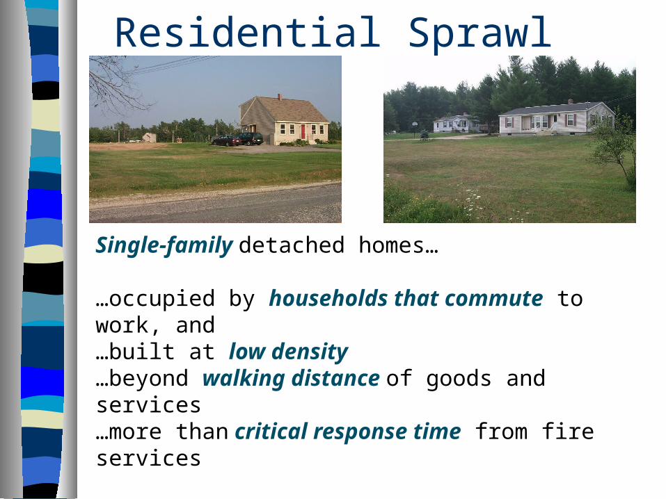
Residential Sprawl

Single-family detached homes…

…occupied by households that commute to work, and …built at low density…beyond walking distance of goods and services…more than critical response time from fire services

Heavy reliance on private automobiles as the primary transportation mode

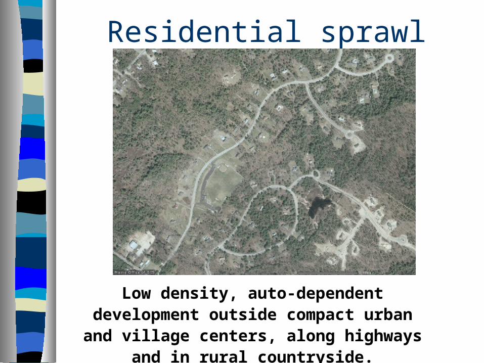
Residential sprawl

Low density, auto-dependent development outside compact urban and village centers,

along highways and in rural countryside.

No centralized planning or control of land uses

Significant fiscal disparities among localities

Reliance on a “trickle-down” or filtering process to provide housing to low-income housholds

Urban Sprawl

7

Urban sprawl “Leapfrog" development which occurs when

developers choose to build on less expensive land farther away from the city, bypassing vacant land located closer to the city

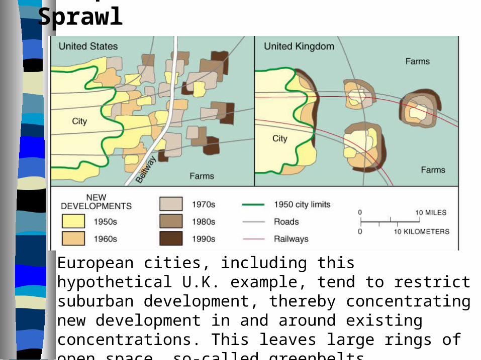
Europe versus U.S. Cities: Sprawl

European cities, including this hypothetical U.K. example, tend to restrict suburban development, thereby concentrating new development in and around existing concentrations. This leaves large rings of open space, so-called greenbelts.

Segregation of land use types into different zones

Strip or ribbon development, which involves extensive commercial development in a linear pattern, which contributes to traffic congestion

Urban Sprawl

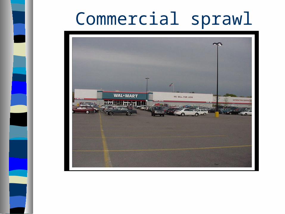
Commercial sprawl

Auto-oriented development…

…built at a low floor area ratio…in strips along major routes or in isolated business parks…separated from other land uses.

Commercial sprawl

ADVANTAGES AND DISADVANTAGES OF SPRAWL

• Social

• Economic

• Environmental

• Health

• ….

ADVANTEGES OF SPRAWL

Advantages improvement of life quality in range of flat (housing

estate with block of flats vs. own detached house) improvement of life quality in range of environment

and landscape (housing estate with block of flats vs. own detached house)

nearness of recreation space; improvement of life quality in terms of safety

ADVANTEGES OF SPRAWL

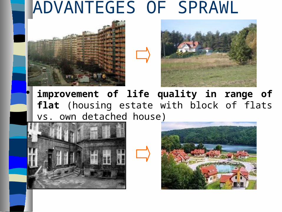
improvement of life quality in range of flat (housing estate with block of flats vs. own detached house)

ADVANTEGES OF SPRAWL

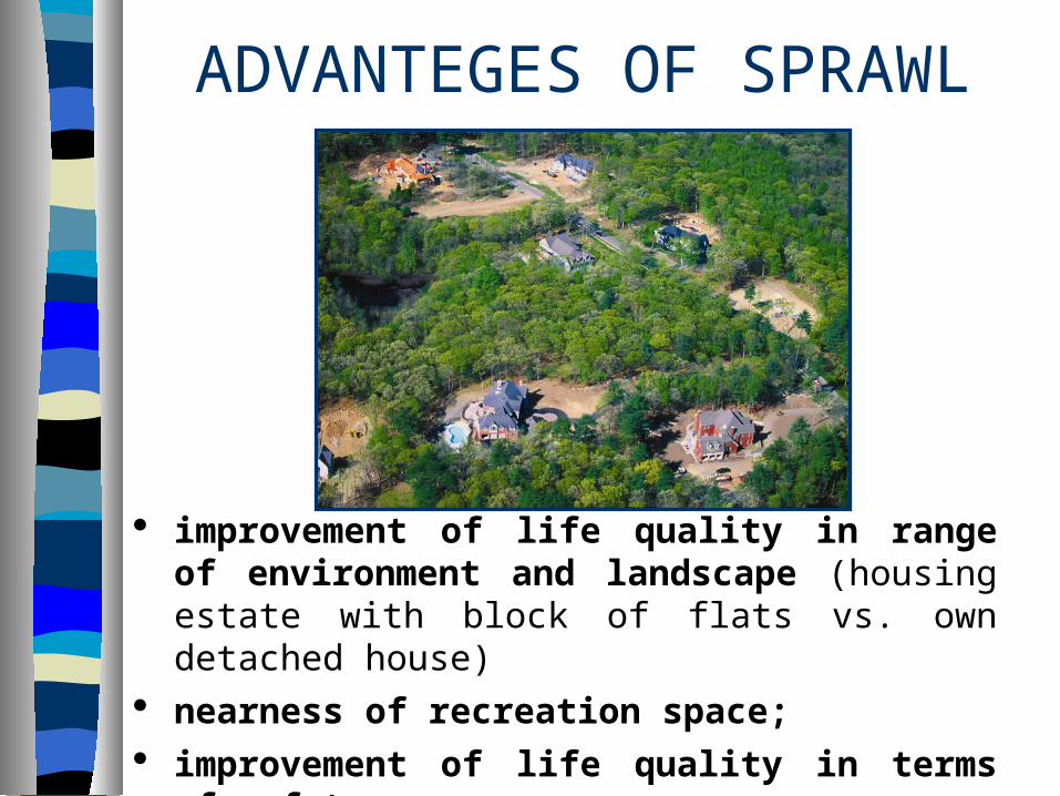
improvement of life quality in range of environment and landscape (housing estate with block of flats vs. own detached house)

nearness of recreation space; improvement of life quality in terms of safety

DISADVANTEGES OF SPRAWL

• Social

• Economical

• Environmental

• Health

• …

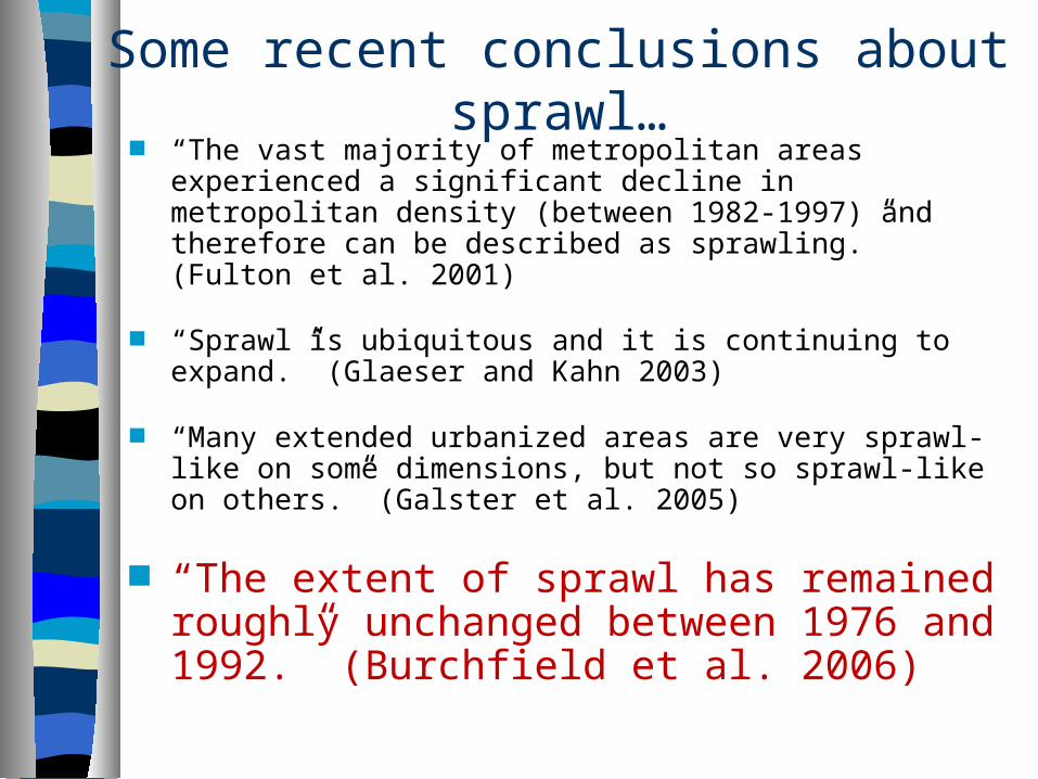
Some recent conclusions about sprawl… “The vast majority of metropolitan areas experienced a

significant decline in metropolitan density (between 1982-1997) and therefore can be described as sprawling.” (Fulton et al. 2001)

“Sprawl is ubiquitous and it is continuing to expand.” (Glaeser and Kahn 2003)

“Many extended urbanized areas are very sprawl-like on some dimensions, but not so sprawl-like on others.” (Galster et al. 2005)

“The extent of sprawl has remained roughly unchanged between 1976 and 1992.” (Burchfield et al. 2006)

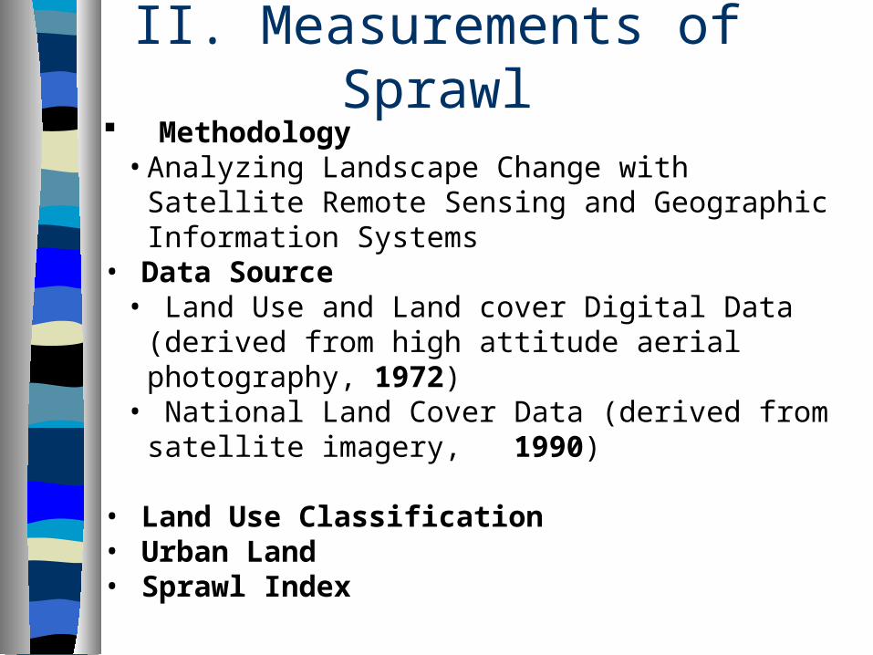
II. Measurements of Sprawl Methodology

• Analyzing Landscape Change with Satellite Remote Sensing and Geographic Information Systems

• Data Source• Land Use and Land cover Digital Data (derived from high

attitude aerial photography, 1972)• National Land Cover Data (derived from satellite

imagery, 1990)

• Land Use Classification• Urban Land• Sprawl Index

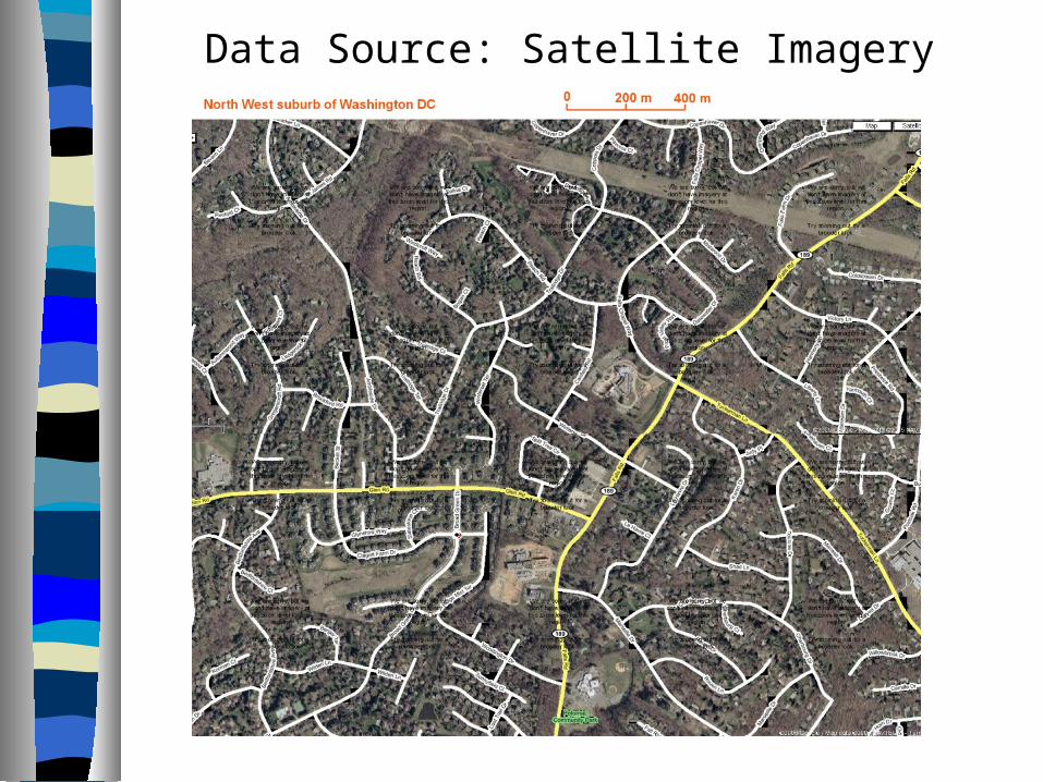
Data Source: Satellite Imagery

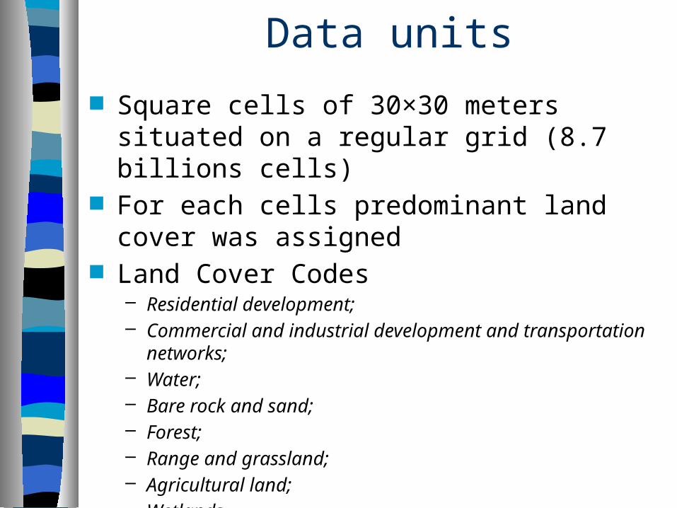
Data units

Square cells of 30×30 meters situated on a regular grid (8.7 billions cells)

For each cells predominant land cover was assigned Land Cover Codes

– Residential development; – Commercial and industrial development and transportation

networks; – Water; – Bare rock and sand; – Forest; – Range and grassland; – Agricultural land; – Wetlands

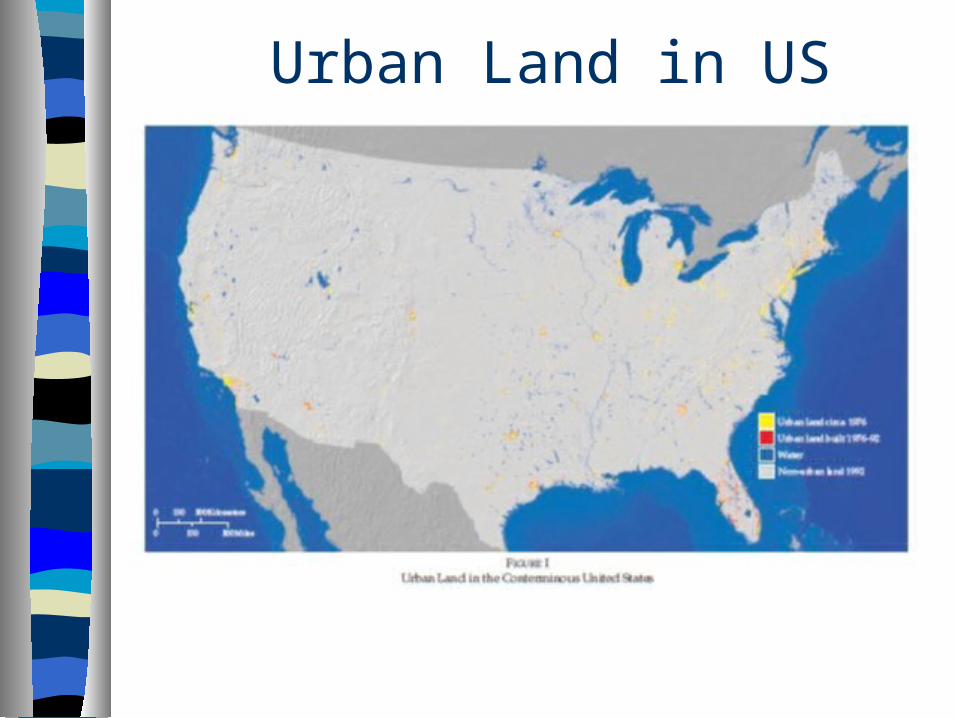
Urban Land in US

Urban Land in US

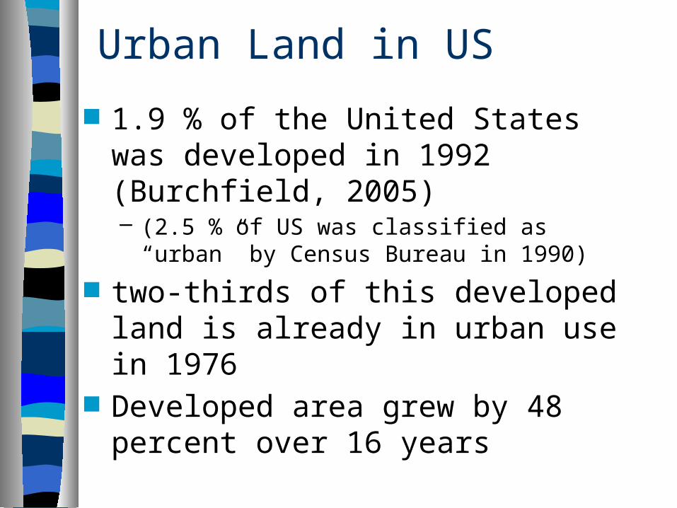
1.9 % of the United States was developed in 1992 (Burchfield, 2005)– (2.5 % of US was classified as “urban” by Census

Bureau in 1990)

two-thirds of this developed land is already in urban use in 1976

Developed area grew by 48 percent over 16 years

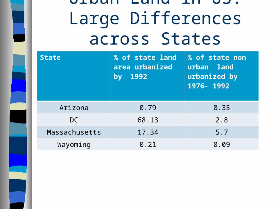
Urban Land in US: Large Differences across States

State % of state land area urbanized by 1992

% of state non urban land urbanized by 1976- 1992

Arizona 0.79 0.35

DC 68.13 2.8

Massachusetts 17.34 5.7

Wayoming 0.21 0.09

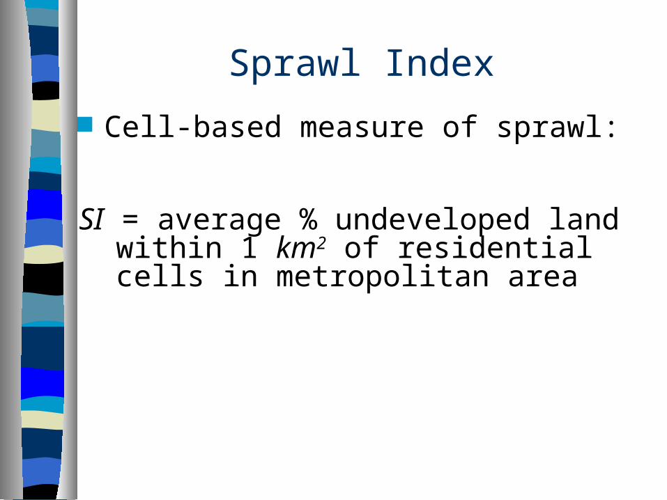
Sprawl Index

Cell-based measure of sprawl:

SI = average % undeveloped land within 1 km2 of residential cells in metropolitan area

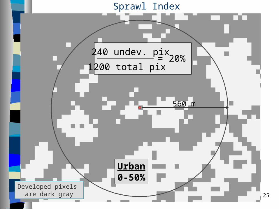
25

240 undev. pix

1200 total pix= 20%

Urban0-50%

Developed pixels are dark gray

560 m

Sprawl Index

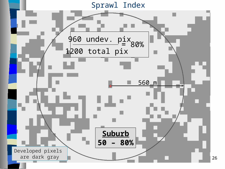
26

960 undev. pix

1200 total pix= 80%

Developed pixels are dark gray

560 m

Sprawl Index

Suburb50 – 80%

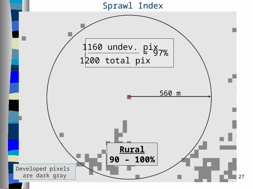
27

1160 undev. pix

1200 total pix= 97%

Rural90 – 100%

Developed pixels are dark gray

560 m

Sprawl Index

Sprawl Index

Spatial scale choice (1 km2 - radius 560 m)– Only 0.3 % of residential development was

more than 1 km from other residential development in 1992

Sprawl Across United states

Sprawl Index (1992) =0.43– Measure of sprawl shows that 43 percent of the

square kilometer surrounding an average residential development is undeveloped

Sprawl Index (1976) =0.42– Average residential development was essentially

unchanged between 1976 and 1992

Sprawl as scattered residential development

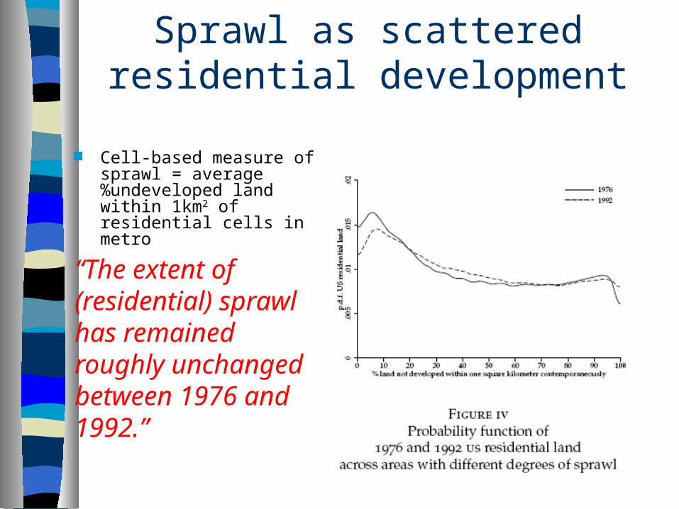
Cell-based measure of sprawl = average %undeveloped land within 1km2 of residential cells in metro

“The extent of (residential) sprawl has remained roughly unchanged between 1976 and 1992.”

Sprawl as scattered residential development

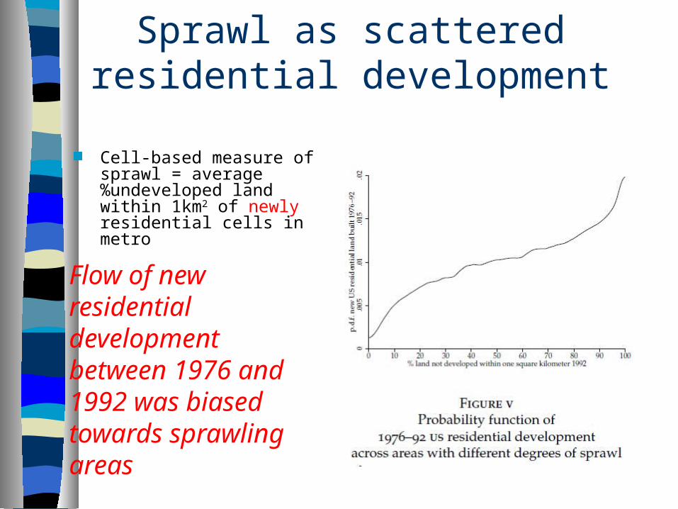
Flow of new residential development between 1976 and1992 was biased towards sprawling areas

Cell-based measure of sprawl = average %undeveloped land within 1km2 of newly residential cells in metro

Sprawl as scattered commercial development

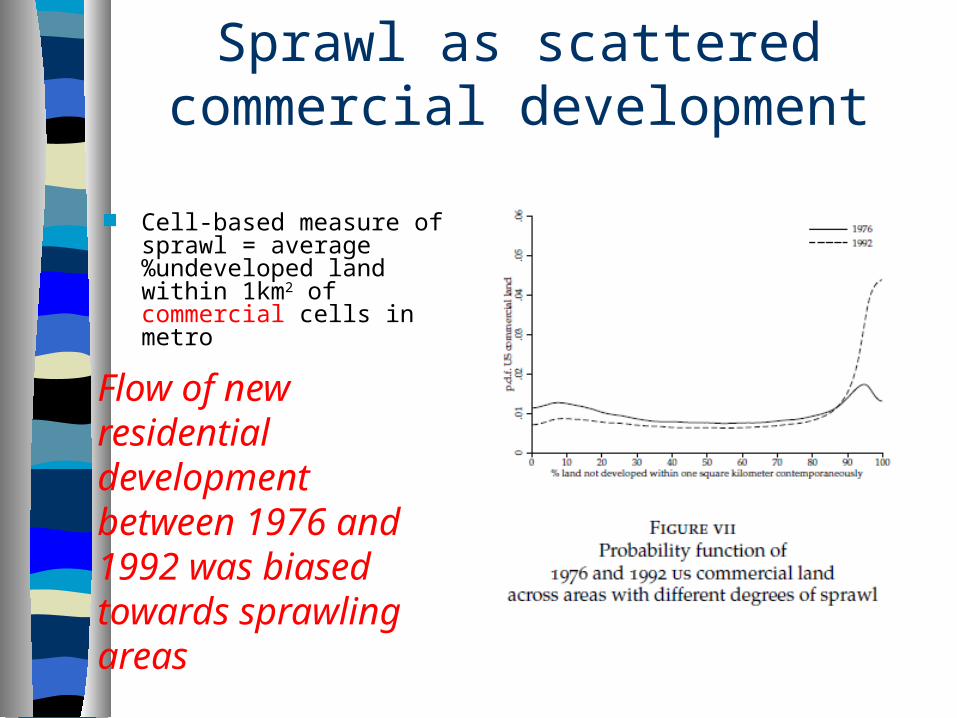
Flow of new residential development between 1976 and1992 was biased towards sprawling areas

Cell-based measure of sprawl = average %undeveloped land within 1km2 of commercial cells in metro

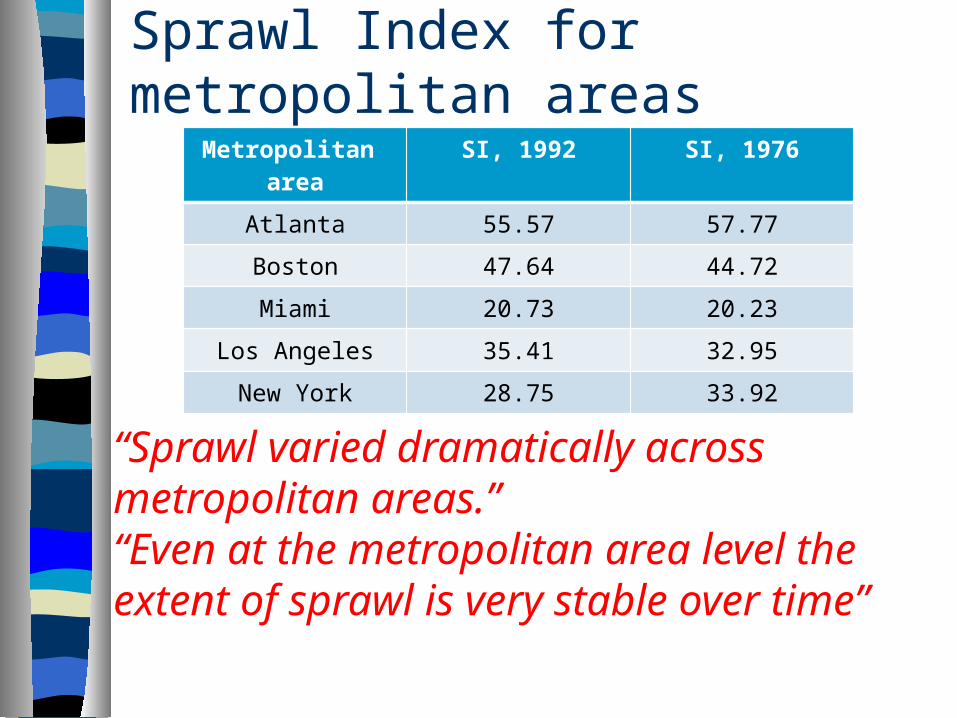
Sprawl Index for metropolitan areas Metropolitan

areaSI, 1992 SI, 1976

Atlanta 55.57 57.77

Boston 47.64 44.72

Miami 20.73 20.23

Los Angeles 35.41 32.95

New York 28.75 33.92

“Sprawl varied dramatically across metropolitan areas.”“Even at the metropolitan area level the extent of sprawl is very stable over time”

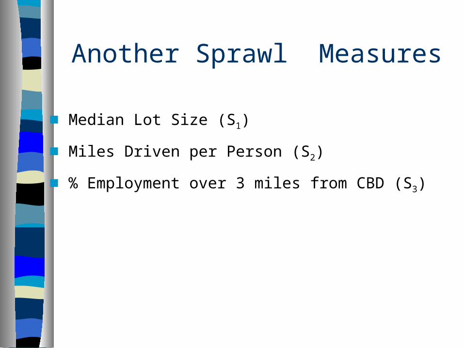
Another Sprawl Measures

Median Lot Size (S1)

Miles Driven per Person (S2)

% Employment over 3 miles from CBD (S3)

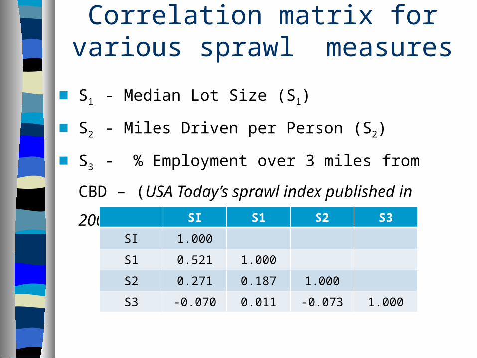
Correlation matrix for various sprawl measures

S1 - Median Lot Size (S1)

S2 - Miles Driven per Person (S2)

S3 - % Employment over 3 miles from CBD – (USA

Today’s sprawl index published in 2001)

SI S1 S2 S3

SI 1.000

S1 0.521 1.000

S2 0.271 0.187 1.000

S3 -0.070 0.011 -0.073 1.000

Urban sprawl variables (other authors)

Residential density Neighborhood mix of homes, jobs, and services; Accessibility of the street network. Overall mobility Public transport Road traffic Accessibilities Strength of activity centers and downtowns ...

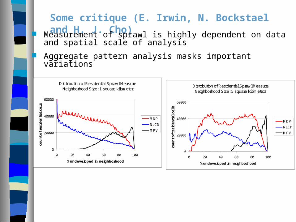
Distribution of Residential Sprawl MeasureNeighborhood Size: 1 square kilometer

0

20000

40000

60000

0 20 40 60 80 100

%undeveloped in neighborhood

cou

nt

of

resi

den

tial

cel

ls

MDP

NLCD

MPV

Distribution of Residential Sprawl MeasureNeighborhood Size: 5 square kilometers

0

20000

40000

60000

0 20 40 60 80 100

%undeveloped in neighborhood

cou

nt

of

resi

den

tial

cel

ls

MDP

NLCD

MPV

Some critique (E. Irwin, N. Bockstael and H. J. Cho)

Measurement of sprawl is highly dependent on data and spatial scale of analysis

Aggregate pattern analysis masks important variations

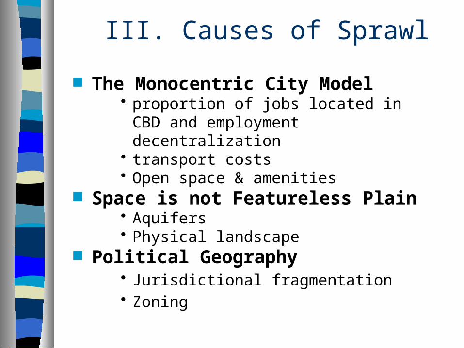
III. Causes of Sprawl

The Monocentric City Model• proportion of jobs located in CBD and

employment decentralization• transport costs• Open space & amenities

Space is not Featureless Plain• Aquifers • Physical landscape

Political Geography• Jurisdictional fragmentation• Zoning

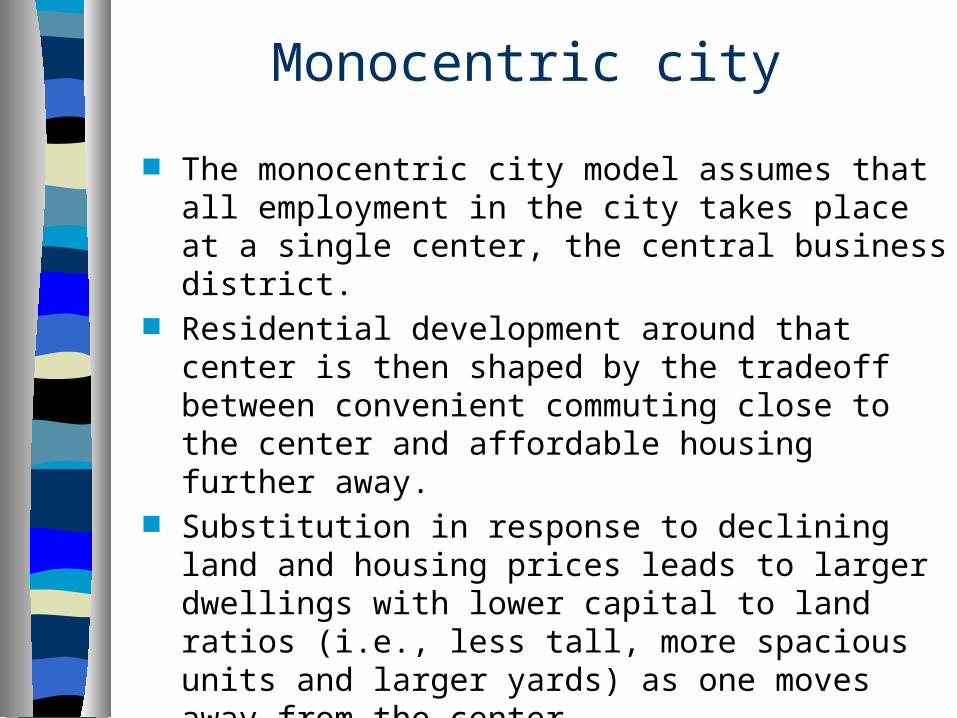
Monocentric city

The monocentric city model assumes that all employment in the city takes place at a single center, the central business district.

Residential development around that center is then shaped by the tradeoff between convenient commuting close to the center and affordable housing further away.

Substitution in response to declining land and housing prices leads to larger dwellings with lower capital to land ratios (i.e., less tall, more spacious units and larger yards) as one moves away from the center.

Monocentric city

Cities specializing in sectors where employment tends to be more centralized will be more compact.

Lower transport costs within a city will result in more dispersed development.

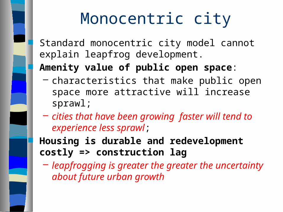
Monocentric city Standard monocentric city model cannot explain leapfrog

development. Amenity value of public open space:

– characteristics that make public open space more attractive will increase sprawl;

– cities that have been growing faster will tend to experience less sprawl;

Housing is durable and redevelopment costly => construction lag– leapfrogging is greater the greater the uncertainty about

future urban growth

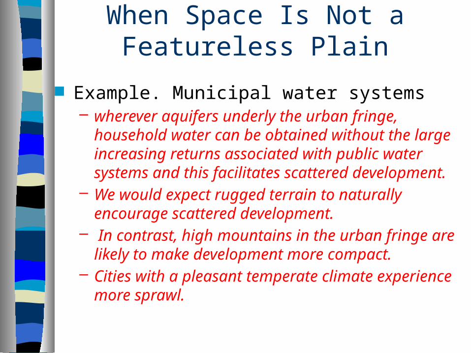
When Space Is Not a Featureless Plain

Example. Municipal water systems– wherever aquifers underly the urban fringe, household

water can be obtained without the large increasing returns associated with public water systems and this facilitates scattered development.

– We would expect rugged terrain to naturally encourage scattered development.

– In contrast, high mountains in the urban fringe are likely to make development more compact.

– Cities with a pleasant temperate climate experience more sprawl.

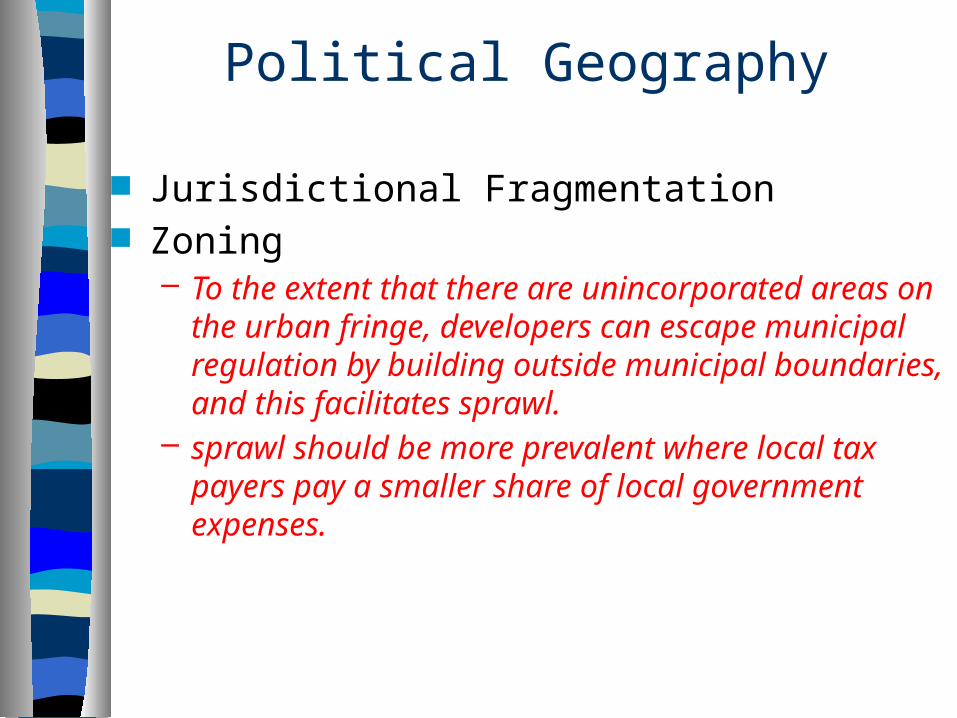
Political Geography

Jurisdictional Fragmentation Zoning

– To the extent that there are unincorporated areas on the urban fringe, developers can escape municipal regulation by building outside municipal boundaries, and this facilitates sprawl.

– sprawl should be more prevalent where local tax payers pay a smaller share of local government expenses.

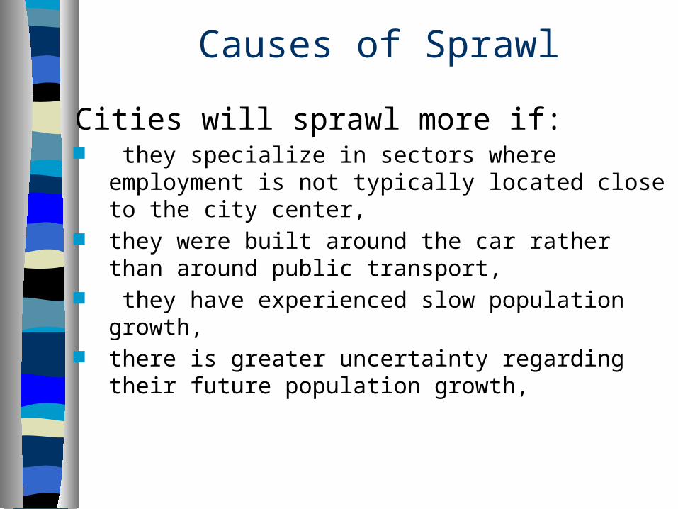
Causes of Sprawl

Cities will sprawl more if: they specialize in sectors where employment is not typically

located close to the city center, they were built around the car rather than around public

transport, they have experienced slow population growth, there is greater uncertainty regarding their future population

growth,

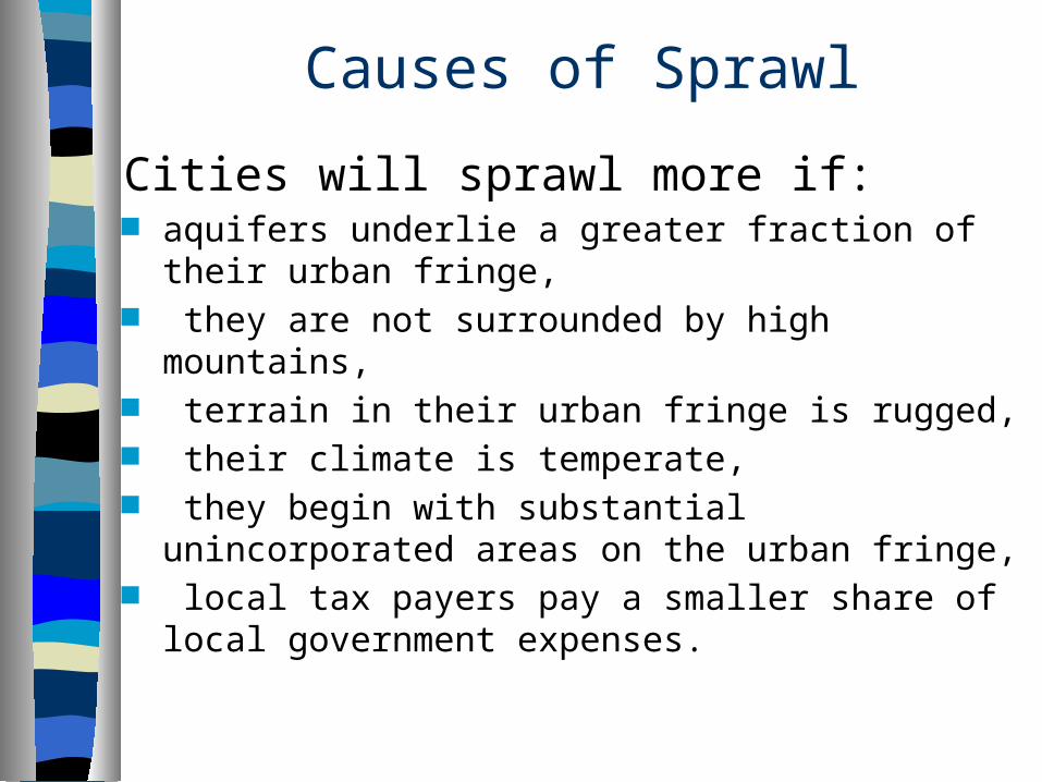
Causes of Sprawl

Cities will sprawl more if: aquifers underlie a greater fraction of their urban fringe, they are not surrounded by high mountains, terrain in their urban fringe is rugged, their climate is temperate, they begin with substantial unincorporated areas on the urban

fringe, local tax payers pay a smaller share of local government

expenses.

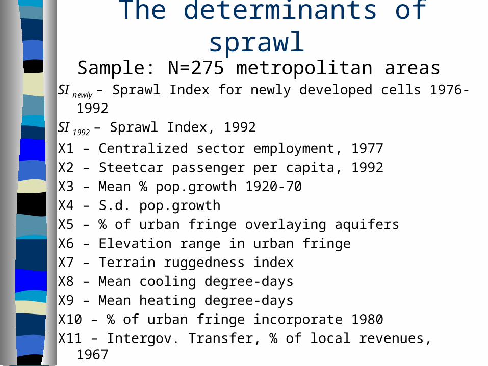
The determinants of sprawl

Sample: N=275 metropolitan areas SI newly – Sprawl Index for newly developed cells 1976-1992

SI 1992 – Sprawl Index, 1992

X1 – Centralized sector employment, 1977

X2 – Steetcar passenger per capita, 1992

X3 – Mean % pop.growth 1920-70

X4 – S.d. pop.growth

X5 – % of urban fringe overlaying aquifers

X6 – Elevation range in urban fringe

X7 – Terrain ruggedness index

X8 – Mean cooling degree-days

X9 – Mean heating degree-days

X10 – % of urban fringe incorporate 1980

X11 – Intergov. Transfer, % of local revenues, 1967

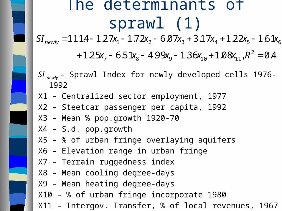
The determinants of sprawl (1)

SI newly – Sprawl Index for newly developed cells 1976-1992

X1 – Centralized sector employment, 1977

X2 – Steetcar passenger per capita, 1992

X3 – Mean % pop.growth 1920-70

X4 – S.d. pop.growth

X5 – % of urban fringe overlaying aquifers

X6 – Elevation range in urban fringe

X7 – Terrain ruggedness index

X8 – Mean cooling degree-days

X9 – Mean heating degree-days

X10 – % of urban fringe incorporate 1980

X11 – Intergov. Transfer, % of local revenues, 1967

4.0,08.136.199.451.625.1

61.122.117.307.672.127.14.1112

1110987

654321

Rxxxxx

xxxxxxSInewly

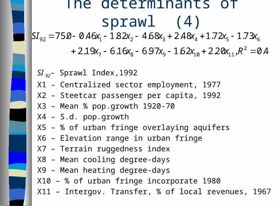
The determinants of sprawl (4)

SI 92– Sprawl Index,1992

X1 – Centralized sector employment, 1977

X2 – Steetcar passenger per capita, 1992

X3 – Mean % pop.growth 1920-70

X4 – S.d. pop.growth

X5 – % of urban fringe overlaying aquifers

X6 – Elevation range in urban fringe

X7 – Terrain ruggedness index

X8 – Mean cooling degree-days

X9 – Mean heating degree-days

X10 – % of urban fringe incorporate 1980

X11 – Intergov. Transfer, % of local revenues, 1967

4.0,20.262.197.616.619.2

73.172.148.268.482.146.00.752

1110987

65432192

Rxxxxx

xxxxxxSI