CAUSES AND CONTROL OFCONCRETE PIPE CORROSION

J .B . Neethling*R.A. Mah**

M.K. Stenstrom*

Annual Report Submitted to the County SanitationDistricts of Los Angeles County

* Civil Engineering Department** School of Public HealthUniversity of CaliforniaLos Angeles, CA 90024

June 1989

TABLE OF CONTENTS

SUMMARY vi

i

PART I. HYDROGEN SULFIDE PRODUCTION IN SEWERS

OBJECTIVES AND APPROACH 1

HYDROGEN SULFIDE PRODUCTION IN SEWERS 2

Hydrogen Sulfide Production Models 2Reactions in a Sewer - An Overview 3Sulfate Reducing Bacteria 4

Organisms and Biochemistry 4Carbon Sources - Electron Donors 4Sulfur Sources - Electron Acceptors 6Environmental Impacts 8

Other Microorganisms 9Sulfide Reactions 10

Weak Acid/Base Chemistry 10Precipitation and Complexation of Sulfides 12Chemical Sulfide Oxidation 13

Mass Transfer Between Gas and Liquid Phase 14

Hydrogen Sulfide Stripping 15Oxygen Transfer - Reaeration 15

Mass Transfer Between Liquid Phase and Biofilm 16

Biofilm Description 16Biofilm Kinetics 16

Kinetic Considerations for a Sewer Pipe Flow Model 21

Growth of Sulfur Reducing Bacteria 21Growth of Aerobic Bacteria 22Dissolved Sulfide Reactions 22Total Sulfide Species 22Dissolved Oxygen 23Organic Substrate 23Inhibitors 24

Reported Sulfide Production Studies 24

Shape of Sulfide Production Studies 24Lag Period 24Correlation Between Sulfate Reduction and Sulfide Production25Impact of Seeding 26

Reaction Precedence - A Summary Model 26

MATERIALS AND METHODS 26

H2SPP Test Protocol 26H2SPP Test Kinetics 29

First Order Kinetics 29Maximum H2S Production Rate 30

Sewer Sampling 31Metal Addition for H2SPP Tests 31

RESULTS AND DISCUSSION 32

Initial H2S in Collected Samples 32H2SPP of Wastewater 32Impact of Biofilm on H2SPP 33Impact of Added Mixture 34

SIGNIFICANCE OF RESULTS 35

NOMENCLATURE 36

REFERENCES 37

APPENDIX A. DATA 41

PART II. SULFATE-REDUCING BACTERIA IN CONCRETE SEWER PIPES

MATERIALS AND METHODS 43

RESULTS AND DISCUSSION 46

PROPOSAL TO LA COUNTY ON SRB 52

REFERENCES 53

PART III. ESTIMATION VOLATILIZATION OF REDUCED SULFUR COMPOUNDS

OCCURRENCE AND SOURCES OF VSCs 68

Monitoring Results for VSCs 68Sources of VSC in Wastewater Treatment Systems 69

11

MASS TRANSFER 71

Mass Transfer Models 71Stripping of Highly Volatile Compounds 73Stripping of Intermediate and Low Volatility Compounds75Calculation of Molecular Diffusivities 76Experimental Verification 78Summary 81

CALCULATING VSC TRANSFER COEFFICIENTS 83

Summary 87

DESCRIPTION OF THE COMPUTER MODEL 89

Summary 92

REFERENCES 93

ill

SUMMARYSulfate reducing bacteria that thrive in sewers while reducing sulfur compounds to produce

hydrogen sulfide. The hydrogen sulfide eventually escapes from the wastewater into the air spaceabove the liquid, where sulfur oxidizing bacteria oxidize sulfide to sulfuric acid . In order to controlthe production of sulfuric acid and the corresponding corrosion, we investigated several aspects ofthe sulfur cycle .

This report consists of three parts. Part I describes the factors that control sulfur reductionin the sewer liquid and slime layers . The bacteriological, chemical, and physical aspects of sulfurreduction is summarized, and laboratory tests performed to measure hydrogen sulfide productionrates, and the impact of additives on the hydrogen sulfide production rate . Part II describes aninvestigation into the microbiology of sulfur reducing bacteria, their growth requirements, and theimpact of selected inhibitors on the growth characteristics of these organisms . Part III investigatedthe mass transfer of volatile compounds (such as hydrogen sulfide or other organic compounds)from the wastewater in a flowing sewer into the gas phase .

iv

PART I. HYDROGEN SULFIDE PRODUCTION IN SEWERS'Hydrogen sulfide (H2S) is produced by sulfur reducing bacteria (SRB) in wastewater flowing

down a sewer. The evolution of H2S in the air space above the wastewater depends on a series ofreactions starting with bacterial sulfur reduction to produce H2S(,0 in the liquid and ending with themass transfer of H2S(, 0 to H2S in the gas phase. The reaction rates and equilibria that control thisprocess are complex and still poorly understood . Besides factors such as pH, temperature, and sewageorganic strength, one needs to incorporate stream velocity and the impact of specific compounds inthe liquid on sulfide reactions and bacterial growth.

This section reviews the factors that contribute to or control H 2S formation in sewage . A lab-oratory test to measure H2S formation in the sewage (called the H2SPP test) is described and used tomeasure the impact of some of these variables on H2S production. Finally, a sewer model is suggestedthat can be used to transfer the H2SPP test results to actual field conditions and applications . Thisreport concentrates on H2S production in sewers . Several literature reviews on sewer corrosion areavailable (for example US EPA 1985 ; Thistlethwayte, 1972) for a more broader and general referenceon sewer corrosion.

OBJECTIVES AND APPROACH

The objective of this study is to determine those factors that contribute significantly to H2Sformation in sewage. Specifically, we attempt to discern the extent to which recent changes in thesewage composition in LA County Sanitation Districts sewers could enhance H 2S formation. The twomost significant changes in wastewater composition are a reduction of metals due to recently imposedsewer discharge regulations, and the addition of waste activated sludge from upstream wastewatertreatment plants .

A test procedure to measure the potential for H2S production in sewage is used to evaluate theimpact of various sewage constituents on H 2S formation. This laboratory test measures H2S formationin sewage over an extended period of time . The rate of and potential for H2S production is measured.Using this test, the impact of metals, inhibitors, toxicants, bacterial densities, etc . can easily be evaluatedand the impact of various components assessed . Before the results are transferred to field conditions,other phenomena such as biofilm kinetics and mass transfer rates from the wastewater to the air spacemust be addressed. The latter aspects can easily be incorporated in a proposed sewer model .

*J.B. Neethling, Xiao Zhang

rs =MiC e-20)son (1)

where

r,

= Rate of sulfide generation in the biofilm, g/m 2-h

M,

= Effective sulfide flux coefficient for sulfide generated in slime, m/h

CBOD

= BOD concentration in wastewater, mg/L

O

= Temperature coefficient, usually O = 1 .07

Equation 1 only accounts for sulfide generation in the biofilm, which is considered to be theprimary source of H2S production . The coefficient, M,, is approximately 3 .2x 104 m/h for partiallyfull pipes and 1 x 10"3 m/h for full flowing pipes .

Thistlethwayte's (1972) model is slightly more complex :

rs = M2VCBODCS OT-20

HYDROGEN SULFIDE PRODUCTION IN SEWERS

Hydrogen Sulfide Production Models

Several models have been proposed to evaluate H2S production in sewers. These models predictthe H2S. concentration in the air space and therefore combine H2S production and evolution kinetics .The Pomeroy and Parkhurst (1977) model is often used . For partially full flow conditions, this modelproposes that the rate of sulfide production in the biofilm can be written as :

(2)

where

M2

= Sulfide production rate coefficient

V

= Stream flow velocity, m/h

CSO4

= Sulfate concentration, mg/L

In Thistlethwayte's model, sulfide generation also depends on the sulfate concentration andstream flow velocity . Their temperature coefficient (© = 1 .139) is significantly higher than thatproposed by Pomeroy and Parkhurst .

While some other variations of these two models are available (ex . Boon and Lister, 1974) thecomponents are essentially the same: H2S evolution in a sewer under field conditions is determinedby the organic strength of the wastewater, temperature, sulfate concentration in some cases, and streamvelocity. In subsequent sections, the impact of these components is investigated in terms of a theoreticaldescription of H2S formation and the kinetics of the sewer system .

2

Reactions in a Sewer - An OverviewFigure 1 shows the classic depiction of a partially filled sewer, containing wastewater with a

variety of organic and sulfur compounds . Commonly, the sewer is half full and the pipe velocitymaintained at approximately 0.6 m/s. Silt and heavy organic particles deposit on the bottom, whilebacterial growth develops on the walls of the sewer to form a biofilm or slime layer . This silt layerand biofilm provide an excellent environment for bacterial growth while protected from the velocityshear forces exerted by flowing wastewater . This model sewer contain several microenvironments :the space above the liquid is commonly filled with air with an abundance of oxygen ; the liquid can beeither aerobic or anaerobic, depending on the oxygen demand and reaeration rates ; the silt and biofilmlayers can also be aerobic or anaerobic .

Anaerobic LayerAerobic Layer

The sulfur cycle in a sewer is fairly well understood . Sulfur compounds such as sulfate, S04- ,is reduced to H2S by sulfur reducing bacteria in an environment depleted of oxygen, in the flowingwastewater or biofilm. H2S in the liquid escapes as a gas into the air space, where reduced sulfur isoxidized by sulfur oxidizing bacteria to produce sulfuric acid .

This report focus on the production of H2S. The following aspects are considered :

•

The bacteriological factors controlling the growth of sulfur reducing bacteria, including inhi-bitors such as oxygen, metals, etc .

•

The wastewater chemistry as it controls reactions between reduced sulfur and other constituentsin the liquid, including precipitation, pH effects, etc .

•

The transfer of H2S from the liquid phase into the gas phase .

3

Sulfate Reducing BacteriaThis section discusses those environmental and nutritional factors that control the growth of

sulfur reducing bacteria in wastewater, and the sequence of events required for bacterial H 2S production.

Organisms and Biochemistry

Sulfur reducing bacteria are obligate anaerobic bacteria that require not only the absence ofoxygen, but also a low redox potential for growth . In the absence of the ideal environment, sulfideproduction will not occur . The sulfur reducing reaction can be depicted as follows :

Organic substrate + Oxidized-S - C02+HZS

(3)

Lactate is a commonly used organic substrate, while sulfate is the dominant oxidized sulfursource. Equation 3 then becomes :

2CH3CHOHCOOH + SO4 -4 2CH3COOH + S'+ 2H20 + 2CO2

According to equation 4, the organic substrate requirement for sulfate reduction is 5.6 mglactate/mg SO4- -S. In terms of the oxygen equivalent (as COD) it therefore requires 6 .0 mg COD/mgS04--S reduced, or also 6 .0 mg COD/mg H2S-S produced. SRBs are quite versatile and will use avariety of carbon sources as substrate as discussed in the next section .

In addition to organic substrate oxidation, several organisms contain the enzyme dehydrogenasewhich catalyze the following reaction to produce H 2S :

4H2 +SO-4S-+4H2O

(5)

These reactions are quite reminiscent of the methane formation reactions encountered inanaerobic digestors .

Carbon Sources - Electron Donors

Sulfur reducing bacteria are quite versatile and can grow effectively on a number of carbonsources. Postgate (1984) proposed lactate as carbon source for a growth medium, but other carbonsources can also be utilized. This is important when we consider growth and H2S production in sewers,since the organic constituents in the wastewater, typically expressed as BOD or COD, may or may notbe available for bacterial growth if the organisms require a particular carbon compound for growth .Pomeroy and Bowlus (1946) suggested that BOD may not be an appropriate measure of availableorganic substrate for predicting H 2S production in sewers, since they observed much higher H2Sproduction in a wastewater containing citrus waste .

Lactate has been considered a prime carbon substrate for SRBs . However, studies into the impactof lactate on H2S production have failed to show that high lactate levels per se in wastewater willenhance H2S formation. Heukelekian (1948) investigated the impact of added lactate on H 2S pro-duction. In pure cultures, added lactate dramatically increased HA production . However, adding

4

(4)

lactate to sterilized wastewater inoculated with SRBs from pure culture, failed to produce H 2S. Nielsenand Hvitved-Jacobsen (1988) tested the ability of biofilms grown on various wastewaters to use dif-ferent carbon source for S04 reduction . They found that feeding lactate as sole carbon source resultedin only 30 to 50% of the H2S production observed when feeding a control with the complex wastewaterused for establishing the biofilm. This means that one single type of carbon source does not accountfor all H2S formation.

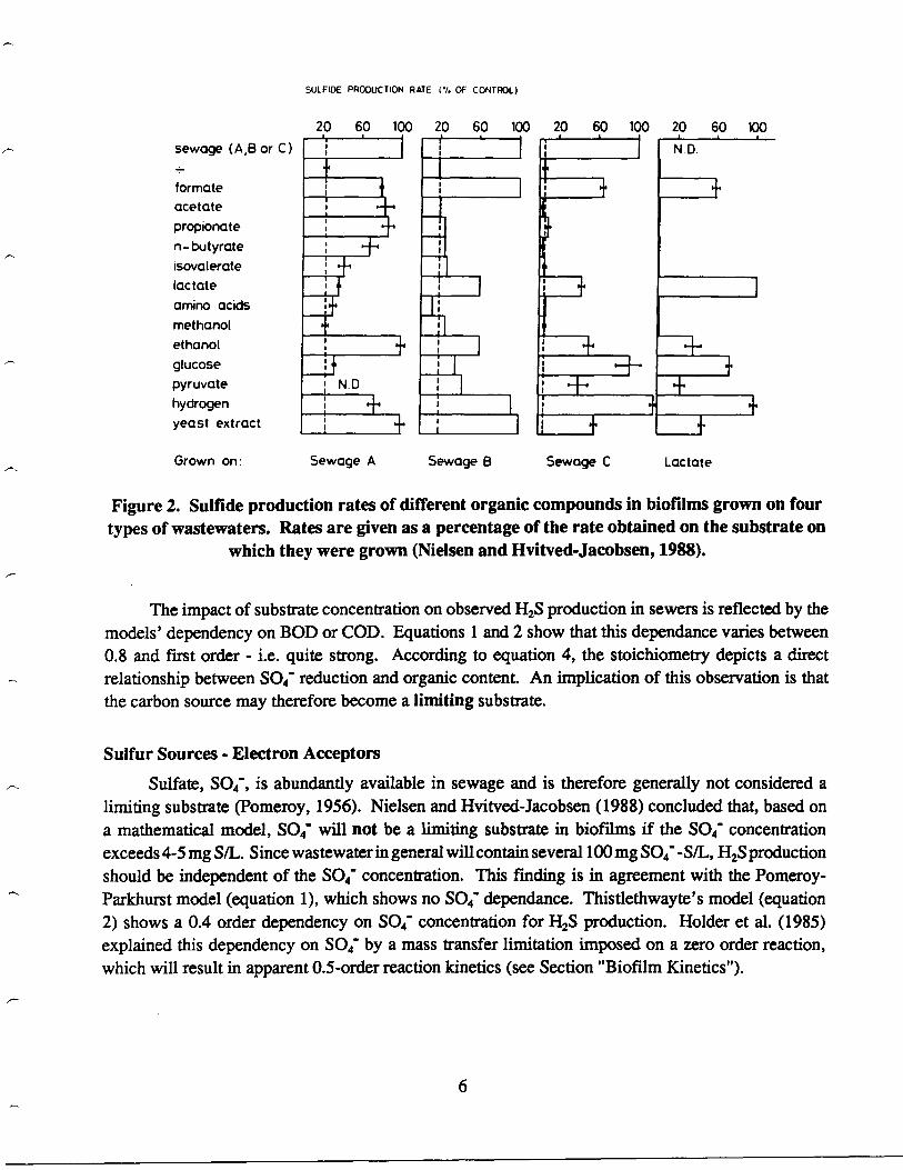
Nielsen and Hvitved-Jacobsen (1988) conducted a study into the impact of selected organiccompounds on S04 reduction and H 2S production in a biofilm reactor . Four substrates were used togrow the biofilm : (A) domestic wastewater; (B) wastewater rich in protein compounds ; (C) wastewaterrich in carbohydrates; (D) a synthetic, lactate based wastewater . Once the biofilm was established, asynthetic feed was introduced containing only one carbon source and S04 reduction rates determined.Figure 2 shows their results, where measured S04 reduction rates are expressed as a percentage ofthe S04 reduction rate when the growth substrate is used . Several important observations can bemade:

• In almost all cases S04 reduction rates for a specific carbon source is much slower than that ofthe complex substrate . S04- reduction proceed optimally in the presence of the complex organicsubstrate used for biofilm growth .

• In the case of a wastewater with a particular characteristic (ex . carbohydrate rich), selectedorganics with that same characteristic (ex . glucose) has a more pronounced impact on S04reduction.

•

Hydrogen had a dramatic impact on S04 reduction, indicating dehydrogenase enzyme activity(equation 5) must be included in H2S formation calculations .

While none of these conclusions are surprizing, their implication is very significant : it seemsthat the "natural" substrate present in a wastewater is also the optimal substrate for SRBs to produceH2S . In other words, the organisms that will survive and grow in abundance in the sewer, will adaptto the carbon source in that wastewater and therefore be adapted to use that particular carbon sourcefor SO4- reduction - irrespective of the actual carbon source .

The above conclusion seems rather surprizing in the light of general perceptions, such as, that"stale" wastewater in general is more prone to H 2S production . It may be, however, that H 2S productionin these cases should be traced to other factors, such as increased SRB populations or the activity ofother heterotrophic bacteria consuming oxygen and lowering the redox potential, as will be discussedin Sections "Environmental Impacts" and "Other Microorganisms" . Note also that this conclusiondoes not imply that the H2S production rate for various carbon sources will be the same - on the contrary,it will be very surprizing if various carbon sources does not yield significantly different H 2S productionrates. However, a SRB population established growing on a given carbon source is likely to preferthat carbon source for H 2S production .

5

sewage (A, B or C )

formateacetatepropionaten- butyrate

isovaleratelactateamino acids

methanolethanolglucosepyruvate

hydrogenyeast extract

Grown on

SULFIDE PRODUCTION RATE (7. OF CONTROL)

20 60 100 20 60 100 20

60 100 20

60

11.1T

+,~,

+

I

+

N.D

6

If

)

If

N . D .

IF

Sewage A

Sewage B

Sewage C

Lactate

100

I

Figure 2. Sulfide production rates of different organic compounds in biofilms grown on fourtypes of wastewaters. Rates are given as a percentage of the rate obtained on the substrate on

which they were grown (Nielsen and Hvitved-Jacobsen,1988) .

The impact of substrate concentration on observed H 2S production in sewers is reflected by themodels' dependency on BOD or COD . Equations 1 and 2 show that this dependance varies between0.8 and first order - i.e. quite strong . According to equation 4, the stoichiometry depicts a directrelationship between S04 reduction and organic content . An implication of this observation is thatthe carbon source may therefore become a limiting substrate .

Sulfur Sources - Electron Acceptors

Sulfate, S04- , is abundantly available in sewage and is therefore generally not considered alimiting substrate (Pomeroy, 1956) . Nielsen and Hvitved-Jacobsen (1988) concluded that, based ona mathematical model, SO4 will not be a limiting substrate in biofilms if the S04 concentrationexceeds 45 mg S/L. Since wastewater in general will contain several 100 mg SO4 -S/L, H2S productionshould be independent of the S04 concentration . This finding is in agreement with the Pomeroy-Parkhurst model (equation 1), which shows no S0 4- dependance. Thistlethwayte's model (equation2) shows a 0.4 order dependency on S04- concentration for H2S production. Holder et al . (1985)explained this dependency on S04 by a mass transfer limitation imposed on a zero order reaction,which will result in apparent 0 .5-order reaction kinetics (see Section "Biofrlm Kinetics") .

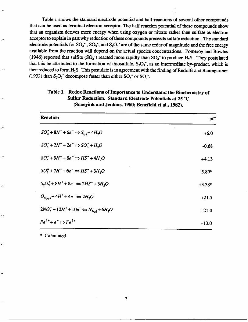
Table 1 shows the standard electrode potential and half-reactions of several other compoundsthat can be used as terminal electron acceptor . The half reaction potential of these compounds showthat an organism derives more energy when using oxygen or nitrate rather than sulfate as electronacceptor to explain in part why reduction of these compounds preceeds sulfate reduction . The standardelectrode potentials for S04 , SO3, and S203' are of the same order of magnitude and the free energyavailable from the reaction will depend on the actual species concentrations . Pomeroy and Bowlus(1946) reported that sulfite (SO3) reacted more rapidly than SO4 to produce H 2S. They postulatedthat this be attributed to the formation of thiosulfate, S 203 as an intermediate by-product, which isthen reduced to form H2S. This postulate is in agreement with the finding of Rudolfs and Baumgartner(1932) than S 203 decompose faster than either S04 or S03 .

Table 1. Redox Reactions of Importance to Understand the Biochemistry ofSulfur Reduction. Standard Electrode Potentials at 25 °C

(Snoeyink and Jenkins, 1980; Benefield et al., 1982) .

7

Reaction PC0

SO4 + 8H + + 6e- t~ S(, ) + 4H20 +6.0

S0 +2H+ +2e- a S0+H2O4

3 -0.68

SO+ 9H+ + 8e- 4*HS- + 4H20 +4.13

S03 + 7H+ + 6e- <* HS- + 3H20 5.89*

S203 + 8H+ + 8e- a 2HS- + 3H2O +3.38*

OA-q) + 4H + + 4e- a 2H20 +21.5

2N03 + 12H + + l0e- t* N2(g )+6H2O +21 .0

Fe 3+ +e- t> Fe2+ +13.0

* Calculated

Environmental Impacts

Redox Potential

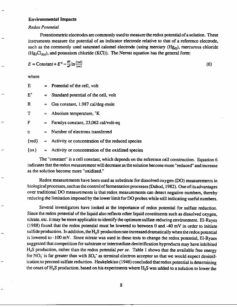
Potentiometric electrodes are commonly used to measure the redox potential of a solution . Theseinstruments measure the potential of an indicator electrode relative to that of a reference electrode,such as the commonly used saturated calomel electrode (using mercury (Hg (j)), mercurous chloride(Hg2C12(,)), and potassium chloride (KC1)). The Nernst equation has the general form :

E =Constant+E°-RTln {ray (6)

where

E

= Potential of the cell, volt

E° = Standard potential of the cell, volt

R = Gas constant, 1 .987 cal/deg-mole

T

= Absolute temperature, °K

F

= Faradys constant, 23,062 cal/volt-eq

n

= Number of electrons transferred

{red} = Activity or concentration of the reduced species

{ox} = Activity or concentration of the oxidized species

The "constant" is a cell constant, which depends on the reference cell construction . Equation 6indicates that the redox measurement will decrease as the solution become more "reduced" and increaseas the solution become more "oxidized ."

Redox measurements have been used as substitute for dissolved oxygen (DO) measurements inbiological processes, such as the control of fermentation processes (Dahod, 1982) . One of its advantagesover traditional DO measurements is that redox measurements can detect negative numbers, therebyreducing the limitation imposed by the lower limit for DO probes while still indicating useful numbers .

Several investigators have looked at the importance of redox potential for sulfate reduction .Since the redox potential of the liquid also reflects other liquid constituents such as dissolved oxygen,nitrate, etc . it may be more applicable to identify the optimum sulfate reducing environment. El-Rayes(1988) found that the redox potential must be lowered to between 0 and -40 mV in order to initiatesulfide production. In addition, the H2S production rate increased dramatically when the redox potentialis lowered to -100 mV. Since nitrate was used in these tests to change the redox potential, El-Ryaessuggested that competition for substrate or intermediate denitrification byproducts may have inhibitedH2S production, rather than the redox potential per se . Table 1 shows that the available free energyfor NO3" is far greater than with SO4- as terminal electron acceptor so that we would expect denitrif-ication to preceed sulfate reduction . Heukelekian (1946) concluded that redox potential is determiningthe onset of H2S production, based on his experiments where H2S was added to a solution to lower the

8

redox potential. He postulated that the onset of H2S production is primarily determined by the activityof other organisms in the wastewater, which lowers the redox potential in the liquid, making H2Sproduction possible .

Temperature

Temperature plays a significant role in all biological reactions. Baumgartner (1934) found thatH2S production virtually ceased at 7 °C. Not only does an increase in temperature increase the rate ofbiochemical reactions, it also controls the growth rate of organisms, thus having a pronounced impacton the bacterial population density .

Sulfide production models often assume a 1.07x'20) factor for temperature impact. This "magic"number can be traced back to the Pomeroy and Bowlus (1946) report, which found a 7% increase inthe maximum H2S production rate . It is questionable whether the same temperature dependency canbe expected for H2S production at other than maximum H2S production rates . For example, Baum-gartner (1934) found little difference in H 2S production patterns for samples kept at 30 and 37 .5 °C .

Other Microorganisms

The nutrient rich environment in a sewer provides ideal conditions for the growth of a wholehost of bacteria. These organisms play an important role in creating an appropriate environment forH2S production by removing potential inhibitors to H 2S production. Of primary importance are thefollowing :

• Aerobic organisms that use 02, N03, and other compounds as electron acceptor . It is wellrecognized that the presence of 02 and NO3 will prevent H2S production in sewers so that theremoval rate of these compounds controls the onset of H 2S production . Aerobic organisms aretherefore of great importance since they create a suitable environment for S04 reduction byremoving 02, NO3, and other inhibitory compounds. Oxygen depletion by aerobic organismsmay therefore be the key to sulfate reduction.

• Fermentative organisms that convert complex organic molecules to more readily accessibleorganic substrates. It was pointed out earlier (see Section "Carbon Sources - Electron Donors")that the actual organic substrate for S04 reduction is probably of less importance due to theversatility of SRBs . Furthermore, fermentative bacteria will only come to play when the redoxpotential is already favorable for H 2S production . However, fermentation which will proceedin the internal biofilm layers, produce fatty acids as byproduct . The fatty acids are the preferredsubstrate for many SRBs and readily biodegradable by aerobic organisms thus sustaining theaerobic activity in the sewer and preventing natural aeration from raising the DO enough toterminate H2S production in the sewer .

The importance of these organisms can only be judged by using a comprehensive sewer modelthat will account for the uptake and growth rates of all the organisms involved . This model mustconsider sequential fermentation and degradation, as well as the "competative" reactions involvingsubstitute electron acceptors such as 02 and N03--

9

Sulfide ReactionsThe mere production if H2S(,, in the wastewater itself, does not mean that H2S will appear in

the gas phase. This section first presents reactions between sulfur compounds and various constituentsin the wastewater, and then address H2S transfer from the liquid to the gas phase .

Weak Acid/Base Chemistry

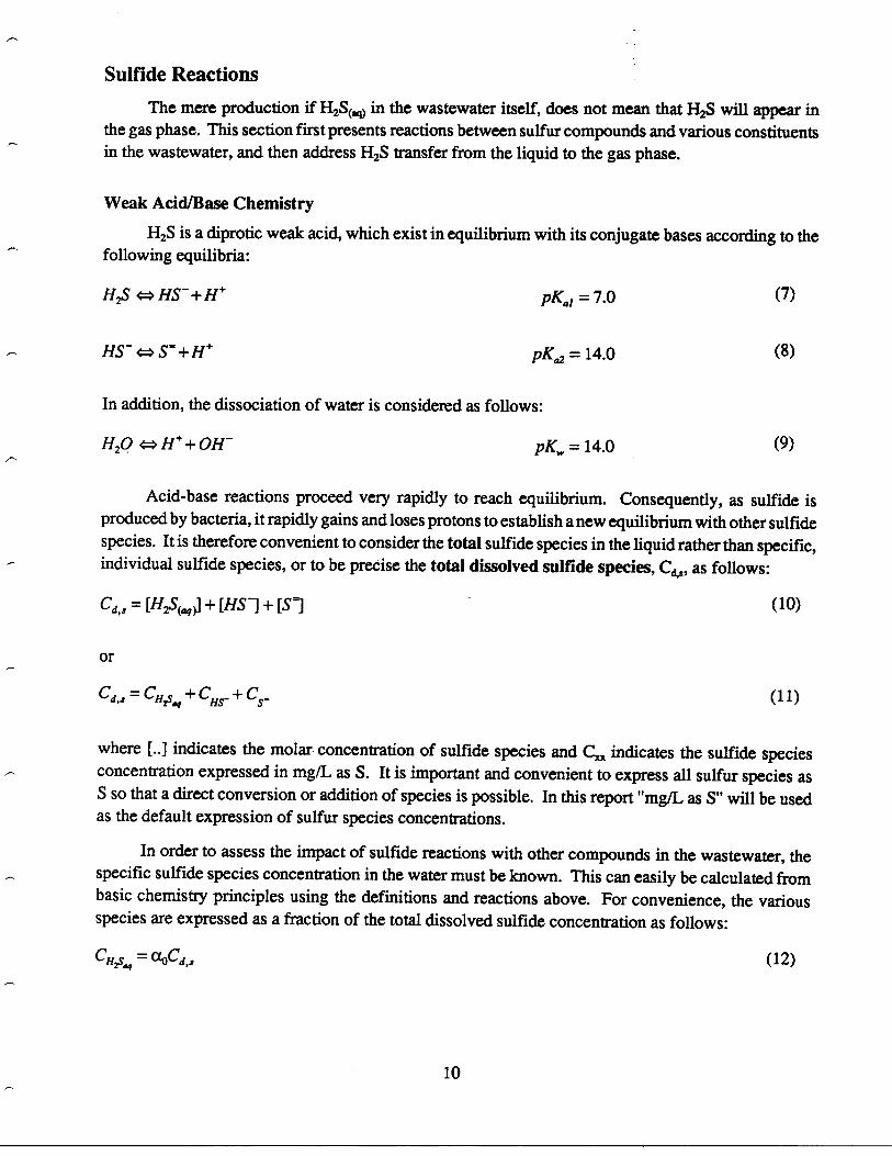
H2S is a diprotic weak acid, which exist in equilibrium with its conjugate bases according to thefollowing equilibria:

Acid-base reactions proceed very rapidly to reach equilibrium . Consequently, as sulfide isproduced by bacteria, it rapidly gains and loses protons to establish a new equilibrium with other sulfidespecies. It is therefore convenient to consider the total sulfide species in the liquid rather than specific,individual sulfide species, or to be precise the total dissolved sulfide species, Cds, as follows :

Cds = [H2S( ) + [HS -I + [S7

or

Cd.,, = CH SIV + CHs- + Cs_

(11)

where [ . .] indicates the molar concentration of sulfide species and C,... indicates the sulfide speciesconcentration expressed in mg/L as S . It is important and convenient to express all sulfur species asS so that a direct conversion or addition of species is possible . In this report "mg/L as S" will be usedas the default expression of sulfur species concentrations .

In order to assess the impact of sulfide reactions with other compounds in the wastewater, thespecific sulfide species concentration in the water must be known . This can easily be calculated frombasic chemistry principles using the definitions and reactions above . For convenience, the variousspecies are expressed as a fraction of the total dissolved sulfide concentration as follows :

Cy2saq = cc OCds

10

H2S t* HS- + H+ pK,d = 7.0 (7)

HS- a S- + H+ pKo2 = 14.0 (8)

In addition, the dissociation of water is considered as follows :

H2O t= H+ + OH-

pKw = 14.0 (9)

CXS_ = alCd , 3

CS_ = a2Cd.,

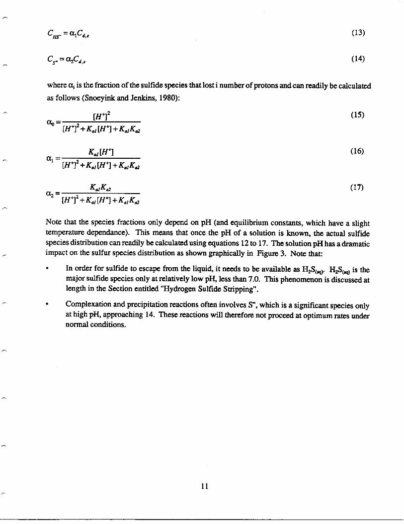
wherea; is the fraction of the sulfide species that lost i number of protons and can readily be calculatedas follows (Snoeyink and Jenkins, 1980) :

av =[H+]2

[H+]2+ K,, [H +] + K,,Ko2

K,, [H*]

al _ [H+]2+K,,[H+]+K,,Ka2

K,,Ka2OC2 =

[H+]2 +K,, [H+] +K,,K,2

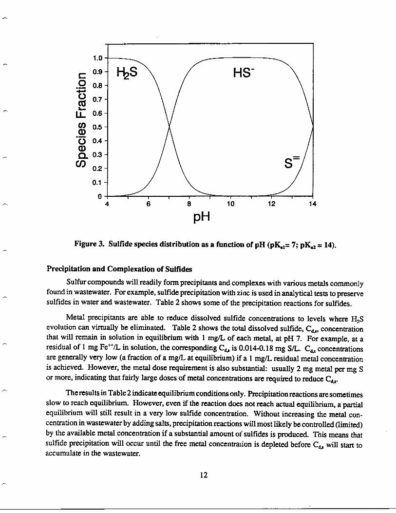
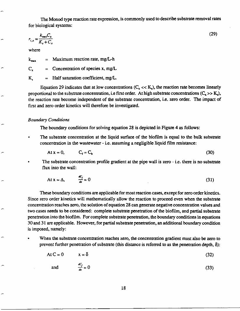
Note that the species fractions only depend on pH (and equilibrium constants, which have a slighttemperature dependance) . This means that once the pH of a solution is known, the actual sulfidespecies distribution can readily be calculated using equations 12 to 17 . The solution pH has a dramaticimpact on the sulfur species distribution as shown graphically in Figure 3 . Note that:

• In order for sulfide to escape from the liquid, it needs to be available as H2S(,q). H2S(,q) is themajor sulfide species only at relatively low pH, less than 7 .0 . This phenomenon is discussed atlength in the Section entitled "Hydrogen Sulfide Stripping" .

• Complexation and precipitation reactions often involves S", which is a significant species onlyat high pH, approaching 14 . These reactions will therefore not proceed at optimum rates undernormal conditions .

1 1

C0

U0LU

CO)CD

0a)CL

1 .0

0.9-

0.8-

0.7-

0.6-

0.5-

0.4-

0.3-

0.2-

0.1 -

0-

I

,

4

10

12

14

pH

Figure 3. Sulfide species distribution as a function of pH (pK . 1= 7; pKaz = 14) .

Precipitation and Complexation of Sulfides

Sulfur compounds will readily form precipitants and complexes with various metals commonlyfound in wastewater. For example, sulfide precipitation with zinc is used in analytical tests to preservesulfides in water and wastewater. Table 2 shows some of the precipitation reactions for sulfides .

Metal precipitants are able to reduce dissolved sulfide concentrations to levels where H2Sevolution can virtually be eliminated . Table 2 shows the total dissolved sulfide, C O, concentrationthat will remain in solution in equilibrium with 1 mg/L of each metal, at pH 7 . For example, at aresidual of 1 mg Fe'/L in solution, the corresponding CO is 0.014-0.18 mg SIL. CO concentrationsare generally very low (a fraction of a mg/L at equilibrium) if a 1 mg/L residual metal concentrationis achieved. However, the metal dose requirement is also substantial : usually 2 mg metal per mg Sor more, indicating that fairly large doses of metal concentrations are required to reduce Co.

The results in Table 2 indicate equilibrium conditions only . Precipitation reactions are sometimesslow to reach equilibrium. However, even if the reaction does not reach actual equilibrium, a partialequilibrium will still result in a very low sulfide concentration . Without increasing the metal con-centration in wastewater by adding salts, precipitation reactions will most likely be controlled (limited)by the available metal concentration if a substantial amount of sulfides is produced . This means thatsulfide precipitation will occur until the free metal concentration is depleted before C d,, will start toaccumulate in the wastewater.

1 2

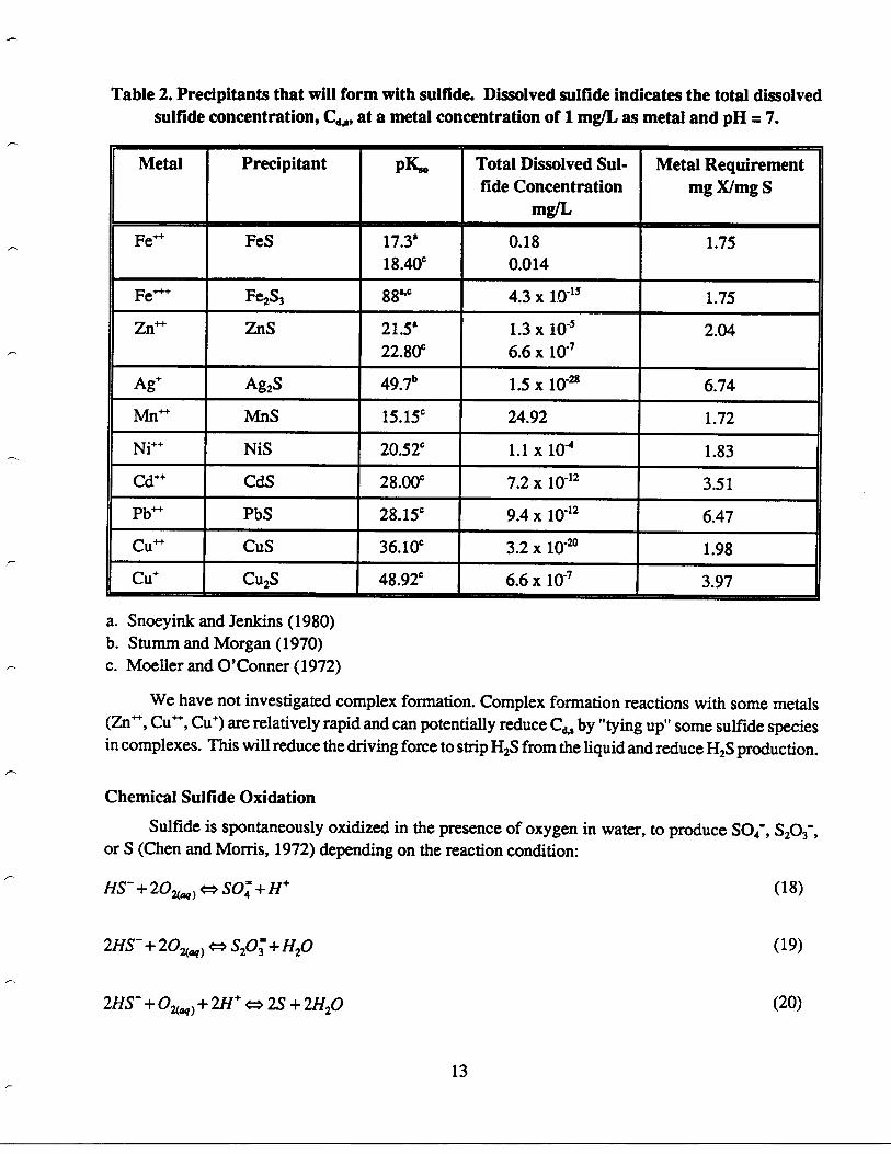
Table 2. Precipitants that will form with sulfide. Dissolved sulfide indicates the total dissolvedsulfide concentration, C0, at a metal concentration of 1 mg/L as metal and pH = 7.

a. Snoeyink and Jenkins (1980)b. Stumm and Morgan (1970)c. Moeller and O'Conner (1972)

We have not investigated complex formation. Complex formation reactions with some metals(Zn++, Cu', Cu') are relatively rapid and can potentially reduce C o by "tying up" some sulfide speciesin complexes. This will reduce the driving force to strip H 2S from the liquid and reduce H2S production.

Chemical Sulfide Oxidation

Sulfide is spontaneously oxidized in the presence of oxygen in water, to produce S04 , S203 - ,or S (Chen and Morris, 1972) depending on the reaction condition :

1 3

Metal Precipitant pK,o Total Dissolved Sul-fide Concentration

mg/L

Metal Requirementmg X/mg S

Fe++ FeS 17.3'18.40c

0.180.014

1 .75

Fe+++ Fe2S3 88',° 4.3 x 1.0-15 1 .75

Zn++ ZnS 21 .5'22.80c

1.3 x 10"5

6.6 x 10"'2.04

Ag+ Ag2S 49.7° 1 .5 x 10"28 6.74

Mn++ MnS 15.15` 24.92 1 .72

Ni++ NiS 20.52c 1.1 x 10-4 1 .83

Cd++ US 28.00c 7.2 x 10' 12 3.51

Pb++ PbS 28.15c 9.4 x 10" 12 6.47

Cu, CuS 36.10c 3.2 x 10"20 1 .98

Cu+ Cu2S 48.92c 6.6 x 10-' 3.97

HS- + 202(aq) r* SO4 +H+ (18)

2HS- +202(aq ) r* S20 3=+ H20 (19)

2HS- + 02(aq) +2H+ a 2S +2H20 (20)

These reactions can have an impact on the H 2S evolution rate from the sewer since the producedH2S may not necessarily appear in the air space . Oxidation of H2S can occur at any point where 02 ispresent. For example, while H2S may be produced in the inside layers of the biofilm, an aerobic layerat the biofilm surface or dissolved oxygen in the liquid may oxidize sulfides before it can be transportedto the gas phase. The kinetics of the process must be determined to assess the impact of sulfide oxidationon H2S production . Sulfide oxidation is generally slow, with a half-life on the order of days . However,several transition metals will catalyze the reaction. Chen and Morris (1970) reported that the time foroxidation of 0 .01 M sulfide at pH 8 .65 decreased from several days to a few minutes in the presenceof 104 M Ni'. Since metal and sulfide concentrations in wastewater are much lower, such a dramaticincrease in oxidation rate is unlikely . Under most environmental conditions they found that sulfideoxidation proceeds slowly and that sulfide and oxygen can co-exist in water .

Mass Transfer Between Gas and Liquid Phase

Gerro and Stenstrom's report (Part III) discusses the factors controlling mass transfer betweenthe liquid and gas phases. This discussion focuses primarily on the impact of mass transfer limitationson the production and evolution of H2S into the gas phase .

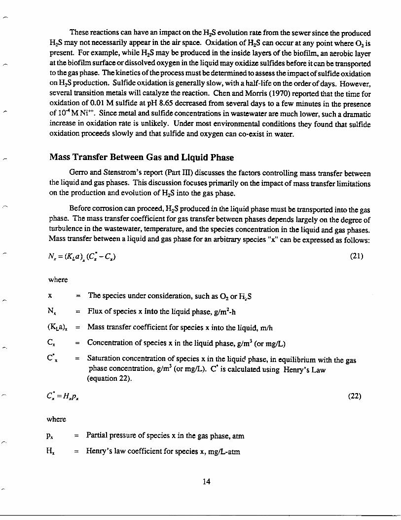
Before corrosion can proceed, H 2S produced in the liquid phase must be transported into the gasphase. The mass transfer coefficient for gas transfer between phases depends largely on the degree ofturbulence in the wastewater, temperature, and the species concentration in the liquid and gas phases .Mass transfer between a liquid and gas phase for an arbitrary species "x" can be expressed as follows :

Ns = (KLa )s (Cx - c )

where

x

= The species under consideration, such as 0 2 or H1.S

NX

= Flux of species x into the liquid phase, g/m2-h

(KLa) x = Mass transfer coefficient for species x into the liquid, m/h

Cx

= Concentration of species x in the liquid phase, g/m3 (or mg/L)

C * X

= Saturation concentration of species x in the liquid phase, in equilibrium with the gasphase concentration, g/m3 (or mg/L) . C* is calculated using Henry's Law(equation 22) .

Cx = Hp.

(22)

where

p x

= Partial pressure of species x in the gas phase, atm

Hx

= Henry's law coefficient for species x, mg/L-atm

14

Henry's Law coefficients are temperature dependant. These expressions for mass transfer cannow be applied to H2S stripping from the liquid and OZ transfer from the gas into the liquid.

Hydrogen Sulfide Stripping

Hydrogen sulfide is a slightly soluble gas . In a sewer, H2S is produced in the liquid phase andthen transported into the gas phase . If we assume the concentration of H 2S in the gas phase is small(see Part III of this report) then C`H2S can be assumed to be zero . The general mass transfer equationis then simplified to :

NH2s = -(KLa)H2SCH2S (23)

The negative sign indicates that the transfer is from the liquid to the gas phase which will cause adecrease in liquid phase concentration .

It is important to note that the transfer rate is dependant on the H 2S(,0 concentration, not the totaldissolved sulfide species . Combining equations 23 and 12, the H2S transfer rate can be written in termsof the total dissolved sulfide concentration :

NH2S = -c o(KLa)H2SCd,+

The transfer H2S rate from the liquid to gas phase is therefore highly dependant on pH (see Figure 3)and only at low pH (<< 7) will the transfer rate proceed at maximum . At pH 7, the H2S transfer ratewill be approximately 50% of the maximum rate . At high pH it is likely that the gas phase H 2Sconcentration will become totally controlled by the mass transfer rates, and equilibrium between thegas and liquid phases will probably not be established . However, even though the transfer rate is lowerat pH > 7, it is not terminated and the potential for H 2S transfer remains the same .

Oxygen Transfer - Reaeration

The DO in the wastewater has a significant and controlling influence on H 2S production sinceH2S production does not occur while 02 is present. Oxygen is also a slightly soluble gas, but unlikeH2S, it is primarily transported from the gas phase into the liquid phase . Aerobic bacteria in thewastewater consumes 02 for metabolism and reduces the DO to virtually zero, when H 2S productionwill commence. If we assume the DO in the liquid phase is small (approximately zero) then C

"O2

controls the mass transfer and the general mass transfer equation is simplified to :

NO2 = +(KLa )O2Co2

or

N02 = +(KLa )O2H02p02

15

(24)

(25)

(26)

The positive sign indicates that 0 2 transfer is from the gas to the liquid phase . This simplified expressionfor reaeration may not be sufficiently accurate to model the sewer due to the importance of the 0 2balance and the need to calculate the DO in the wastewater accurately . It serves here only to illustratethe dominant factors or driving forces for reaeration .

If we assume that the oxygen concentration in the gas phase remains essentially constant (pO2 =0.21 atm) then the reaeration rate becomes solely dependent on the mass transfer coefficient, (KLa)02 .The mass transfer coefficient is controlled by the flow velocity, depth of flow, and temperature (seeGerro and Stenstrom's report, Part III) .

Mass Transfer Between Liquid Phase and Biofilm

Biofilm Description

The biofilm in a sewer contributes significantly to H 2S production in sewers (Holder et al . 1985 ;Nielsen and Hvitved-Jacobsen, 1988 ; Pomeroy and Bowlus, 1946 ; Holder, 1986; El-Rayes, 1988) .This is commonly attributed to two factors : a high SRB population in the biofilm, and an ideal envi-ronment for H2S production .

The bacterial population in the biofilm is significantly greater than that in the bulk liquid (seePart II of this report ; Heukelekian, 1948). This large population on the pipe wall can be attributed tothe stationary surface which prevents bacteria from washing away and allow for a significant populationto develop in the biofilm . Additionally, the liquid's slower velocity at the pipe surface facilitate bacterialadhesion and create a niche for bacterial growth .

The environment inside the biofilm is ideal for H2S production . Diffusional resistances limitoxygen transfer into the biofilm, so that an anaerobic layer develops at the pipe surface . The biofilm(Figure 1) is considered to contain several layers ranging from possibly aerobic on the liquid side, toanaerobic on the pipe side . The actual distribution of oxygen inside the biofilm is determined by theavailability of nutrients in the bulk liquid and the reaction rates in the biofilm itself . Before proceedingwith this discussion, it is important to investigate biofilm kinetics .

Biofilm Kinetics

Reaction rate expressions are commonly derived for homogeneous reactions . These rateexpressions therefore describe the rate at which a particular reaction will proceed in an environmentwhere mass transfer is not limited . Furthermore, the reactions are considered to be homogeneous, i.e .the potential for a reaction is the same at any location inside the liquid . Even though few field scalereactions fall into this strict definition, homogenous reaction rate expressions are used for manypractical applications. Homogeneous reaction rate expressions can be applied to determine biofilmkinetics, as have been studied for areas such as trickling filters . We will use these descriptions for H 2Sproduction in sewers .

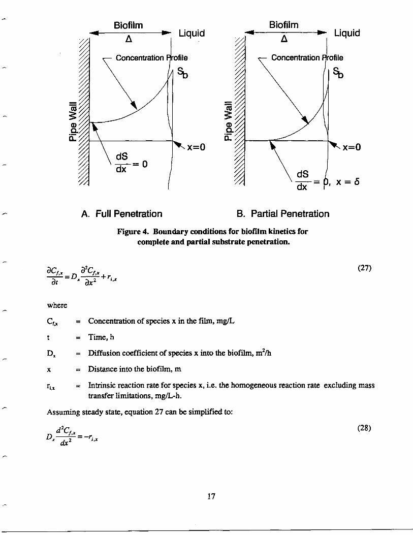
Biofilms in a sewer grow an a reasonable flat surface . The biofilm kinetics can therefore beapproximated by a flat plate geometry . Figure 4 shows a model describing substrate transfer into abiofilm. The process is mathematically described as follows :

16

Biofilm

A. Full Penetration

aCf,x=

a2Cf,.a=

D.,,ax2

+r`s

17

B. Partial Penetration

Figure 4. Boundary conditions for biofilm kinetics forcomplete and partial substrate penetration .

(27)

where

Cf ,,

= Concentration of species x in the film, mg/L

t

= Time, h

D,,

= Diffusion coefficient of species x into the biofilm, m 2/h

x

= Distance into the biofilm, m

r;, x

= Intrinsic reaction rate for species x, i.e. the homogeneous reaction rate excluding masstransfer limitations, mg/L-h .

Assuming steady state, equation 27 can be simplified to :

d2Cf,x

Dsdx2

(28)

The Monod type reaction rate expression, is commonly used to describe substrate removal ratesfor biological systems :

k.xC.

r; z = K3 + Cx

where

k.-, = Maximum reaction rate, mg/L-h

Cx = Concentration of species x, mg/L

K,

= Half saturation coefficient, mg/L .

Equation 29 indicates that at low concentrations (C,, << K,), the reaction rate becomes linearlyproportional to the substrate concentration, i.e first order. At high substrate concentrations (Cx >> K,),the reaction rate become independent of the substrate concentration, i .e. zero order. The impact offirst and zero order kinetics will therefore be investigated .

Boundary Conditions

The boundary conditions for solving equation 28 is depicted in Figure 4 as follows :

©

The substrate concentration at the liquid surface of the biofilm is equal to the bulk substrateconcentration in the wastewater - i.e. assuming a negligible liquid film resistance :

(29)

At x=0, Cf = Cb (30)

©

The substrate concentration profile gradient at the pipe wall is zero - i.e. there is no substrateflux into the wall :

At x = O,

dC' 0

(31)dx

These boundary conditions are applicable for most reaction cases, except for zero order kinetics .Since zero order kinetics will mathematically allow the reaction to proceed even when the substrateconcentration reaches zero, the solution of equation 28 can generate negative concentration values andtwo cases needs to be considered : complete substrate penetration of the biofilm, and partial substratepenetration into the biofilm . For complete substrate penetration, the boundary conditions in equations30 and 31 are applicable. However, for partial substrate penetration, an additional boundary conditionis imposed, namely :

©

When the substrate concentration reaches zero, the concentration gradient must also be zero toprevent further penetration of substrate (this distance is referred to as the penetration depth, 8) :

AtC=0

x=8

(32)

and

~' 0

(33)

18

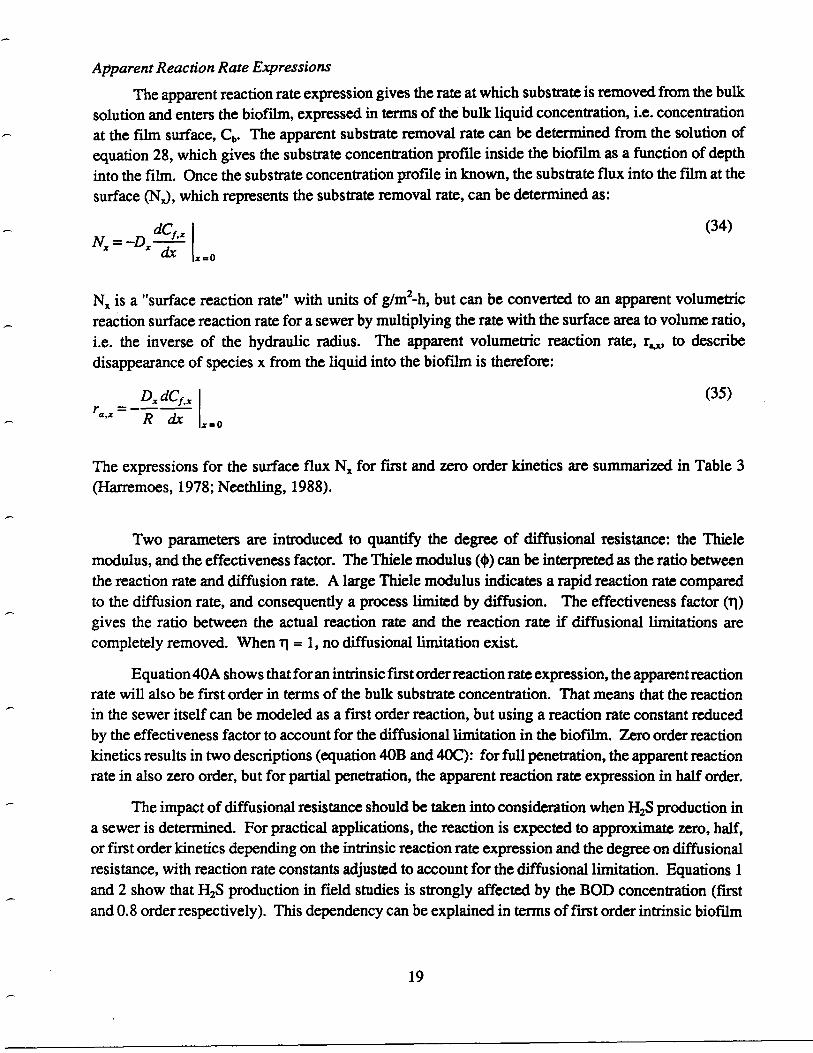
Apparent Reaction Rate ExpressionsThe apparent reaction rate expression gives the rate at which substrate is removed from the bulk

solution and enters the biofilm, expressed in terms of the bulk liquid concentration, i .e. concentrationat the film surface, Cb . The apparent substrate removal rate can be determined from the solution ofequation 28, which gives the substrate concentration profile inside the biofilm as a function of depthinto the film. Once the substrate concentration profile in known, the substrate flux into the film at thesurface (NJ, which represents the substrate removal rate, can be determined as :

Nx = DxdCf

' xdx

_ D. dCf, x'a ,x

R dx

x=0

(34)

Nx is a "surface reaction rate" with units of g/m 2-h, but can be converted to an apparent volumetricreaction surface reaction rate for a sewer by multiplying the rate with the surface area to volume ratio,i.e. the inverse of the hydraulic radius . The apparent volumetric reaction rate, r,,,,, to describedisappearance of species x from the liquid into the biofilm is therefore :

x=0

(35)

The expressions for the surface flux N,, for first and zero order kinetics are summarized in Table 3(Harremoes, 1978 ; Neethling, 1988) .

Two parameters are introduced to quantify the degree of diffusional resistance : the Thielemodulus, and the effectiveness factor . The Thiele modulus (~) can be interpreted as the ratio betweenthe reaction rate and diffusion rate . A large Thiele modulus indicates a rapid reaction rate comparedto the diffusion rate, and consequently a process limited by diffusion . The effectiveness factor (11)gives the ratio between the actual reaction rate and the reaction rate if diffusional limitations arecompletely removed. When r1= 1, no diffusional limitation exist.

Equation 40A shows that for an intrinsic first order reaction rate expression, the apparent reactionrate will also be first order in terms of the bulk substrate concentration . That means that the reactionin the sewer itself can be modeled as a first order reaction, but using a reaction rate constant reducedby the effectiveness factor to account for the diffusional limitation in the biofilm . Zero order reactionkinetics results in two descriptions (equation 40B and 40C) : for full penetration, the apparent reactionrate in also zero order, but for partial penetration, the apparent reaction rate expression in half order .

The impact of diffusional resistance should be taken into consideration when H2S production ina sewer is determined. For practical applications, the reaction is expected to approximate zero, half,or first order kinetics depending on the intrinsic reaction rate expression and the degree on diffusionalresistance, with reaction rate constants adjusted to account for the diffusional limitation . Equations 1and 2 show that H2S production in field studies is strongly affected by the BOD concentration (firstand 0.8 order respectively). This dependency can be explained in terms of first order intrinsic biofilm

19

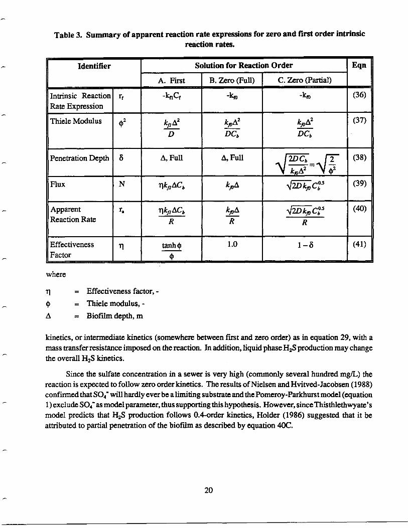
Table 3. Summary of apparent reaction rate expressions for zero and first order intrinsicreaction rates.

where

Ti

= Effectiveness factor, -

4'

= Thiele modulus, -0

= Biofilm depth, m

kinetics, or intermediate kinetics (somewhere between first and zero order) as in equation 29, with amass transfer resistance imposed on the reaction . In addition, liquid phase H2S production may changethe overall H2S kinetics .

Since the sulfate concentration in a sewer is very high (commonly several hundred mg/L) thereaction is expected to follow zero order kinetics . The results of Nielsen and Hvitved-Jacobsen (1988)confirmed that S04 - will hardly ever be a limiting substrate and the Pomeroy-Parkhurst model (equation1) exclude S04 as model parameter, thus supporting this hypothesis . However, since Thisthlethwyate'smodel predicts that H2S production follows 0 .4-order kinetics, Holder (1986) suggested that it beattributed to partial penetration of the biofilm as described by equation 40C .

20

Identifier Solution for Reaction Order Eqn

A. First B. Zero (Full) C. Zero (Partial)

Intrinsic ReactionRate Expression

rf -kf,Cf -km -kfp (36)

Thiele Modulus ,tit`Y kk L2

Dk 42DCb

k 42DCb

(37)

Penetration Depth S 0, Full 0, Full (38)2D Cb -k~e2

,tit`Y

Flux N ilkf1Cb k 4 (39)2DkJ,Cbs

ApparentReaction Rate

ra r)kn1Cb kjv0R

(40)2Dkjv Cb3R R

EffectivenessFactor

rl tanh 4 1 .0 1-8 (41)

10

Kinetic Considerations for a Sewer Pipe Flow ModelA sewer can be modeled in terms of the physical flow and transport of mass, coupled with

appropriate reaction rate expressions . Two types of reactions should be considered : rapid reactions,which can be assumed to be essentially in equilibrium, and slow reactions that must include appropriatekinetics rate expressions. In addition, reactions in both the liquid and biofilm must be included . Fora comprehensive and more complete model, gas phase reactions and gas convection should be added .However, since we are primarily interested in the H2S production rates the gas phase will be assumedto be a non-reactive sink for H2S.

At this point, the kinetic model has not been completely developed in terms ofthe pipe flow model and the relative reaction rates . The focus of the work to date hasbeen to assess the impact of various liquid phase components on the H 2S productionrate, which is essential information needed to formulate and apply the model . Additionaleffort is needed to calibrate and test the model, which we hope to undertake during thenext year.

The following sections describe the relationship between various components of the sewer model(sulfide, sulfate, BOD/COD, DO, etc.), the reactions in which the species are consumed or produced,and their impact on bacterial growth .

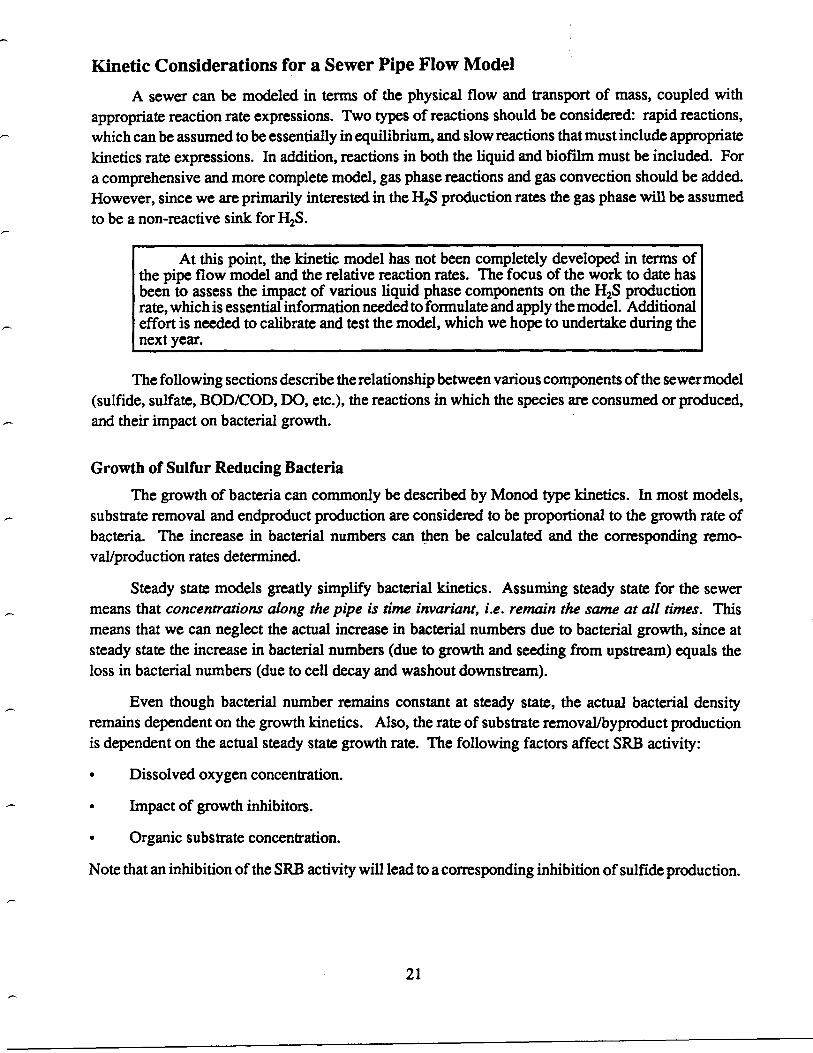
Growth of Sulfur Reducing Bacteria

The growth of bacteria can commonly be described by Monod type kinetics . In most models,substrate removal and endproduct production are considered to be proportional to the growth rate ofbacteria. The increase in bacterial numbers can then be calculated and the corresponding remo-val/production rates determined .

Steady state models greatly simplify bacterial kinetics . Assuming steady state for the sewermeans that concentrations along the pipe is time invariant, i .e . remain the same at all times . Thismeans that we can neglect the actual increase in bacterial numbers due to bacterial growth, since atsteady state the increase in bacterial numbers (due to growth and seeding from upstream) equals theloss in bacterial numbers (due to cell decay and washout downstream) .

Even though bacterial number remains constant at steady state, the actual bacterial densityremains dependent on the growth kinetics . Also, the rate of substrate removal/byproduct productionis dependent on the actual steady state growth rate . The following factors affect SRB activity :

©

Dissolved oxygen concentration .

©

Impact of growth inhibitors .

©

Organic substrate concentration .

Note that an inhibition of the SRB activity will lead to a corresponding inhibition of sulfide production .

21

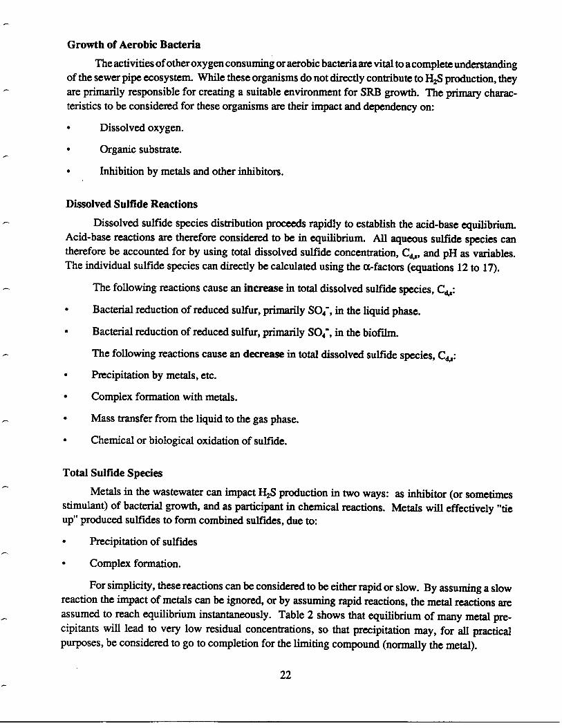
Growth of Aerobic Bacteria

The activities of other oxygen consuming or aerobic bacteria are vital to a complete understandingof the sewer pipe ecosystem. While these organisms do not directly contribute to H 2S production, theyare primarily responsible for creating a suitable environment for SRB growth . The primary charac-teristics to be considered for these organisms are their impact and dependency on :

©

Dissolved oxygen .

©

Organic substrate .

©

Inhibition by metals and other inhibitors .

Dissolved Sulfide Reactions

Dissolved sulfide species distribution proceeds rapidly to establish the acid-base equilibrium .Acid-base reactions are therefore considered to be in equilibrium . All aqueous sulfide species cantherefore be accounted for by using total dissolved sulfide concentration, Cd,,, and pH as variables .The individual sulfide species can directly be calculated using the a-factors (equations 12 to 17) .

The following reactions cause an increase in total dissolved sulfide species, CO:

©

Bacterial reduction of reduced sulfur, primarily S04, in the liquid phase .

©

Bacterial reduction of reduced sulfur, primarily S04- , in the biofilm .

The following reactions cause an decrease in total dissolved sulfide species, Cd,, :

©

Precipitation by metals, etc .

©

Complex formation with metals .

©

Mass transfer from the liquid to the gas phase .

©

Chemical or biological oxidation of sulfide .

Total Sulfide Species

Metals in the wastewater can impact H2S production in two ways : as inhibitor (or sometimesstimulant) of bacterial growth, and as participant in chemical reactions . Metals will effectively "tieup" produced sulfides to form combined sulfides, due to :

©

Precipitation of sulfides

©

Complex formation .

For simplicity, these reactions can be considered to be either rapid or slow. By assuming a slowreaction the impact of metals can be ignored, or by assuming rapid reactions, the metal reactions areassumed to reach equilibrium instantaneously . Table 2 shows that equilibrium of many metal pre-cipitants will lead to very low residual concentrations, so that precipitation may, for all practicalpurposes, be considered to go to completion for the limiting compound (normally the metal) .

22

. The total sulfide concentration in the wastewater consists therefore of two components : dis-solved sulfides, which accounts for the reactive sulfide species that participate in reactions with metalsand are stripped from the liquid, and combined sulfide, which represents precipitated and complexedsulfide species :

C,, s = Cds + Ce , S

where

C4 ,

= Total sulfide concentration, mg/L as S

Cd,,

= Dissolved sulfide concentration, mg/L as S

Cc,,

= Combined sulfide concentration, mg/L as S

Dissolved Oxygen

Dissolved oxygen in the wastewater will practically eliminate H2S production . The followingactivities must be considered to determine DO concentration in the liquid and biofilm :

©

Oxygen consumption by aerobic organisms

©

Reaeration from the gas phase

©

Chemical oxidation of reduced sulfur compounds

©

DO profiles in the biofilm.

Organic Substrate

Organic substrate is commonly measured by the BOD or COD concentration . As pointed outin Section "Carbon Sources - Electron Donors", SRBs are extremely versatile and can use many dif-ferent carbon sources . While lumped parameters such as BOD or COD may not give the actual growthnutrient concentration, it may still be an adequate indicator of the growth nutrient concentration . Thefollowing factors have an impact on the organic substrate concentration :

©

Sulfur reducing bacterial growth

©

Aerobic organisms growth

©

Fermentor activity .

Prolonged exposure to an anaerobic environment can lead to the formation of volatile fatty acids,which can impact H2S production in two ways : (1) Volatile fatty acids have been shown to be anoptimum carbon substrate for SRB activity . (2) If the wastewater subsequently enters an pipe sectionwhere oxygen transfer is increased, the presence of the volatile acids, which are generally more rapidlydegraded by aerobic organisms, will lead to an increase in aerobic activity and hence increased oxygenuptake. The net result is that it may be impossible to maintain aerobic conditions in the aerated pipesection, leading to favorable conditions for SRB growth .

23

(42)

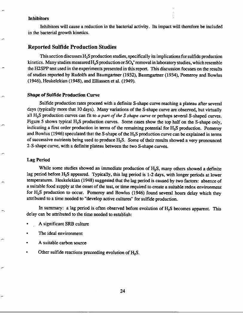
Inhibitors

Inhibitors will cause a reduction in the bacterial activity. Its impact will therefore be includedin the bacterial growth kinetics .

Reported Sulfide Production Studies

This section discusses H2S production studies, specifically its implications for sulfide productionkinetics . Many studies measured H2S production or S04 ` removal in laboratory studies, which resemblethe H2SPP test used in the experiments presented in this report . This discussion focuses on the resultsof studies reported by Rudolfs and Baumgartner (1932), Baumgartner (1934), Pomeroy and Bowlus(1946), Heukelekian (1948), and Elliassen et al . (1949) .

Shape of Sulfide Production Curve

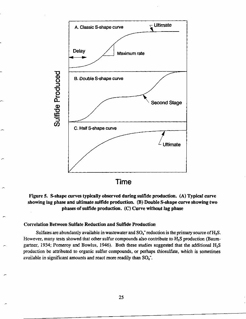
Sulfide production rates proceed with a definite S-shape curve reaching a plateau after severaldays (typically more that 10 days) . Many variations of the S-shape curve are observed, but virtuallyall H2S production curves can fit to a part of the S shape curve or perhaps several S-shaped curves .Figure 5 shows typical H2S production curves. Some cases show the top half on the S-shape only,indicating a first order production in terms of the remaining potential for H 2S production. Pomeroyand Bowlus (1946) speculated that the S-shape of the H 2S production curve can be explained in termsof successive nutrients being used to produce H 2S. Some of their results showed a very pronounced2-S-shape curve, with a definite plateau between the two S-shape curves .

Lag Period

While some studies showed an immediate production of H 2S, many others showed a definitelag period before H2S appeared. Typically, this lag period is 1-2 days, with longer periods at lowertemperatures . Heukelekian (1948) suggested that the lag period is caused by two factors : absence ofa suitable food supply at the onset of the test, or time required to create a suitable redox environmentfor H2S production to occur. Pomeroy and Bowlus (1946) found several hours delay which theyattributed to a time needed to "develop active cultures" for sulfide production .

In summary : a lag period is often observed before evolution of H2S becomes apparent. Thisdelay can be attributed to the time needed to establish :

©

A significant SRB culture

©

The ideal environment

©

A suitable carbon source

©

Other sulfide reactions preceeding evolution of H2S.

24

a)U

0L(-La)Vy--

CI)

A. Classic S-shape curve

Delay-4so-

B. Double S-shape curve

C. Half S-shape curve

Maximum rate

Time

Figure 5. S-shape curves typically observed during sulfide production. (A) Typical curveshowing lag phase and ultimate sulfide production . (B) Double S-shape curve showing two

phases of sulfide production . (C) Curve without lag phase

Correlation Between Sulfate Reduction and Sulfide Production

Sulfates are abundantly available in wastewater and S04` reduction is the primary source of H2S .However, many tests showed that other sulfur compounds also contribute to H2S production (Baum-gartner, 1934; Pomeroy and Bowlus, 1946) . Both these studies suggested that the additional H 2Sproduction be attributed to organic sulfur compounds, or perhaps thiosulfate, which is sometimesavailable in significant amounts and react more readily than S0 4`.

25

Ultimate

Second Stage

Ultimate

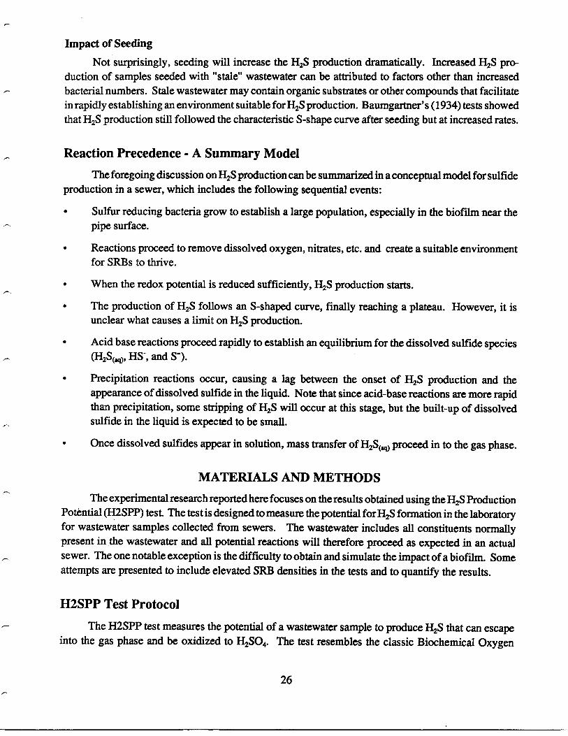
Impact of Seeding

Not surprisingly, seeding will increase the H 2S production dramatically. Increased H2S pro-duction of samples seeded with "stale" wastewater can be attributed to factors other than increasedbacterial numbers. Stale wastewater may contain organic substrates or other compounds that facilitatein rapidly establishing an environment suitable for H2S production . Baumgartner's (1934) tests showedthat H2S production still followed the characteristic S-shape curve after seeding but at increased rates .

Reaction Precedence - A Summary Model

The foregoing discussion on H 2S production can be summarized in a conceptual model for sulfideproduction in a sewer, which includes the following sequential events :

©

Sulfur reducing bacteria grow to establish a large population, especially in the biofilm near thepipe surface.

©

Reactions proceed to remove dissolved oxygen, nitrates, etc. and create a suitable environmentfor SRBs to thrive .

©

When the redox potential is reduced sufficiently, H2S production starts .

©

The production of H2S follows an S-shaped curve, finally reaching a plateau . However, it isunclear what causes a limit on H2S production .

©

Acid base reactions proceed rapidly to establish an equilibrium for the dissolved sulfide species(H2S(4, HS and S`) .

© Precipitation reactions occur, causing a lag between the onset of H 2S production and theappearance of dissolved sulfide in the liquid. Note that since acid-base reactions are more rapidthan precipitation, some stripping of H 2S will occur at this stage, but the built-up of dissolvedsulfide in the liquid is expected to be small .

©

Once dissolved sulfides appear in solution, mass transfer of H2S(,v proceed in to the gas phase.

MATERIALS AND METHODSThe experimental research reported here focuses on the results obtained using the H 2S Production

Potential (H2SPP) test. The test is designed to measure the potential for H2S formation in the laboratoryfor wastewater samples collected from sewers . The wastewater includes all constituents normallypresent in,the wastewater and all potential reactions will therefore proceed as expected in an actualsewer. The one notable exception is the difficulty to obtain and simulate the impact of a biofilm . Someattempts are presented to include elevated SRB densities in the tests and to quantify the results .

H2SPP Test Protocol

The H2SPP test measures the potential of a wastewater sample to produce H 2S that can escapeinto the gas phase and be oxidized to H2SO4. The test resembles the classic Biochemical Oxygen

26

Demand (BOD) test by simply measuring the evolution of H2S from a sample. H2S generated by thesample is captured in a solution containing zinc acetate, which is subsequently analyzed for H2S .Rudolfs and Baumgartner (1932) and Baumgartner (1934) describe similar tests for determining H 2Sproduction. Their procedure is virtually identical to the same procedure discussed here .

The sample is placed in a container to allow bacterial reduction of sulfur compounds to H 2S.After the selected contact time, H2S is stripped from the solution by first lowering the pH to convertall sulfide to H2S(,q) and then bubbling N2W through the sample. The N2 gas leaving the sample iscollected and bubbled through a zinc acetate solution (pH 10) to capture the sulfide . In order to obtainuseful results, a 100% capture efficiency must be achieved in the experimental setup . The impact ofpH, sample volume, and the zinc acetate concentration on capture efficiency were investigated . Theprocedures in Standard Methods (APHA, 1985) for capture and preservation of sulfide samples wasfound adequate to ensure sulfide capture .

Various physical setups for the H2SPP tests were investigated to optimize purge time and captureefficiency. Four H2S capture configurations (Figure 6) using various combinations of flasks andgraduate cylinders were tested . Configuration B (Figure 6) was used to test the capture efficiency offlasks . A solution of sodium sulfide was placed in the "sample" flask and then purged to determinethe capture efficiency . Results in Table 4 show that the efficiency for 3 capture flasks in series usinga purge time of 20 minutes is very good . Less than 20% H2S escapes the first flask . However, it alsoindicates that mass transfer must be overcome in order to increase the capture efficiency for a singlecapture flasc. This hypothesis was tested using cylinders as both capture and sample vessels (Figure6D). The resulting capture efficiency (Table 5) confirm our hypothesis where about 90% or bettercapture was obtained in 10 minutes purge time .

C .

Sample Capture

27

Sample Capture

D.

Capture Capture

Figure 6. Capture configurations for H2SPP test .

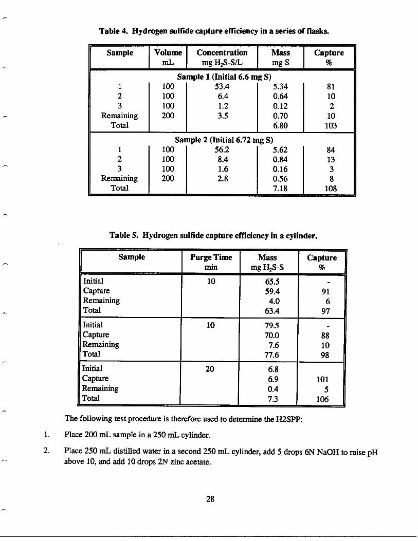
Table 4. Hydrogen sulfide capture efficiency in a series of flasks.

123

RemainingTotal

Sample

123

RemainingTotal

VolumeML

Sa100100100200

Sample 2 (Initial 6.72 m100

56.2100

8.4100

1.6200

2.8

Concentrationmg H2S-S/L

mple 1(Initial 6.6 mg S)53 .4 5.346.4 0.641 .2 0.123.5

0.706.80

Massmg S

g S)5 .620.840.160.567.18

Capture

8110210103

841338

108

Table 5. Hydrogen sulfide capture efficiency in a cylinder .

The following test procedure is therefore used to determine the H2SPP :

1 . Place 200 mL sample in a 250 mL cylinder .

2 .

Place 250 mL distilled water in a second 250 mL cylinder, add 5 drops 6N NaOH to raise pHabove 10, and add 10 drops 2N zinc acetate .

I

28

Sample Purge Timemin

Massmg H2S-S

Capture%

Initial 10 65.5 -Capture 59.4 91Remaining 4.0 6Total 63.4 97

Initial 10 79.5 -Capture 70.0 88Remaining 7.6 10Total 77.6 98Initial 20 6.8Capture 6.9 101Remaining 0.4 5Total 7.3 106

3 .

Connect piping between sample and capture flascs .

4 .

Incubate sample for desired period .

5 . Add 7 drops 6N HCl to the sample flasc to lower pH below 3 .

6.

Purge for 10 minutes with N2 gas .

7 .

Measure the H 2S concentration in the capture volume according to Standard Methods (Method428A) and calculate the H2SPP. Express the results as mg H 2S-S/L based on the sample volume .

This procedure is virtually identical to that described by Rudolfs and Baumgartner (1932) . Themajor differences are: the pH is lowered in the H2SPP test before purging to ensure that all sulfide isconverted to H2S to enhance the stripping efficiency. They did not lower the pH but continued purgingthe sample for 30 to 60 minutes "depending on the amount of sulfide present ." In addition, they usedCO2 gas for purging, whereas we used N 2 .

H2SPP Test Kinetics

Two approaches can be followed to analyze H2SPP data : Previous tests (see Section "Shape ofSulfide Production Curve") indicated that H 2S production typically follows an S-shaped curve . First,if we assume that the initial slow production of H 2S is attributed to a lag phase and this lag is eliminatedduring data analysis, then the process can be described by first order kinetics in terms of the remainingpotential for H2S formation (as in the BOD test) . Alternatively, since the most important part of thereaction for sewer kinetics is the first 12 or 24 hours, the peak H 2S production rate as determined bythe maximum slope of the H2S production curve could be used as measure of the H2S productionpotential in the sewer. Pomeroy and Bowlus (1946) used the maximum H 2S production rate in theirpaper .

First Order Kinetics

In order to determine the ultimate, or maximum, H2SPP, collected data were analyzed in asimilar way as the classic BOD time series analysis . Assume a first order model with respect to theremaining H2SPP:

r3 = - kS

(43)

where

r,

= Reaction rate for H2S production, mg S/L-hr

k

= Reaction rate constant, hf1

S

= H2SPP remaining, mg S/L

Applying equation 43 to a batch reactor between time 0 and time=t, the H2SPP remaining isexpressed as :

29

S =Sue-'b`

where

S• = Ultimate H2SPP, mg S/L

t

= Time, d

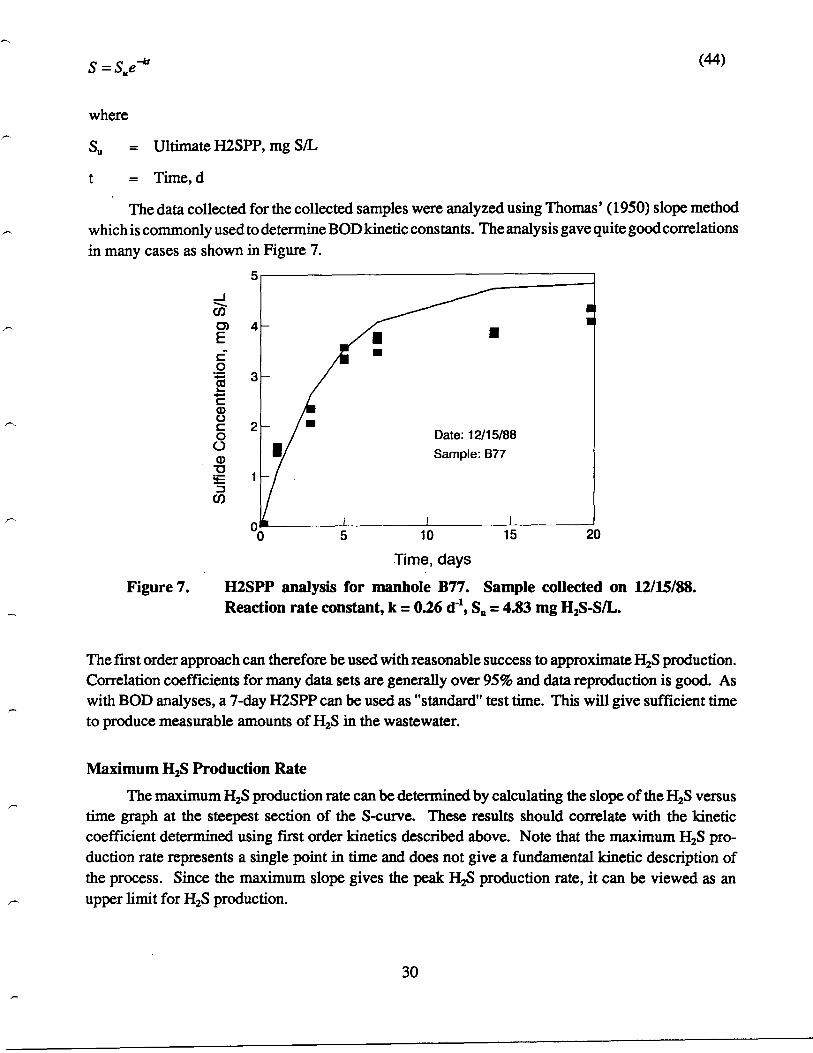
The data collected for the collected samples were analyzed using Thomas' (1950) slope methodwhich is commonly used to determine BOD kinetic constants . The analysis gave quite good correlationsin many cases as shown in Figure 7 .

I I l

5

10

15

20Time, days

Figure 7.

H2SPP analysis for manhole B77 . Sample collected on 12/15/88 .Reaction rate constant, k = 0.26 d"', S• = 4.83 mg H2S-SIL .

The first order approach can therefore be used with reasonable success to approximate H2S production .Correlation coefficients for many data sets are generally over 95% and data reproduction is good . Aswith BOD analyses, a 7-day H2SPP can be used as "standard" test time . This will give sufficient timeto produce measurable amounts of H2S in the wastewater.

Maximum H2S Production Rate

The maximum H2S production rate can be determined by calculating the slope of the H2S versustime graph at the steepest section of the S-curve . These results should correlate with the kineticcoefficient determined using first order kinetics described above . Note that the maximum H2S pro-duction rate represents a single point in time and does not give a fundamental kinetic description ofthe process. Since the maximum slope gives the peak H 2S production rate, it can be viewed as anupper limit for H2S production .

30

(44)

Sewer Sampling

Samples were collected from sewers six times during the year (Table 7) at manholes in twosewer lines. Manholes B77 and B78 are located in a heavily corroded sewer, while manhole E30 islocated in a non-corroded sewer.

Metal Addition for H2SPP Tests

In order to assess the impact of wastewater constituents on H 2S production, a mix of four metalcompounds were added to a wastewater sample and the H2SPP determined. The concentrations ofthe four metal compounds in wastewater decreased rather substantially from 1973 to 1987 as shownin Table 8. Since the actual concentration of these compounds vary significantly in wastewater, atypical concentration was chosen to represent the approximate metal concentration . The metal mixwas added to the wastewater sample, which mean that the true species concentration (Table 8) is theinitial wastewater concentration (which was not measured) plus the added amount . These concentrationvalues are therefore only an approximation of what was present in the sample during the test . However,the measured H2SPP when compared to the control, will give an indication of the impact of the mixon H2S production.

Table 7. Sample dates and locations .

3 1

Date Location

9/22/88 B77

11/10/88 B77

12/15/88 B77

12/15/88 E30

2/9/89 B78

5/3/89 B78

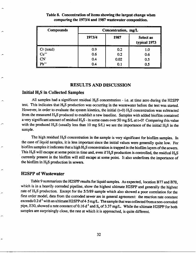
Table 8. Concentration of items showing the largest change whencomparing the 1973/4 and 1987 wastewater composition .

RESULTS AND DISCUSSION

Initial H2S in Collected Samples

All samples had a significant residual H 2S concentration - i.e. at time zero during the H2SPPtest, This indicates that H2S production was occurring in the wastewater before the test was started .However, in order to evaluate the system kinetics, the initial (t=0) H 2S concentration was subtractedfrom the measured H2S produced to establish a new baseline . Samples with added biofilm containeda very significant amount of residual H2S - in some cases over 50 mg S/L at t=0! Comparing this valuewith the produced H2S (usually less than 10 mg S/L) we see the importance of the initial H2S in thesample.

The high residual H2S concentration in the sample is very significant for biofilm samples . Inthe case of liquid samples, it is less important since the initial values were generally quite low . Forbiofilm samples it indicates that a high H 2S concentration is trapped in the biofilm layers of the sewers .This H2S will escape at some point in time and, even if H 2S production is controlled, the residual H2Scurrently present in the biofilm will still escape at some point . It also underlines the importance ofthe biofilm in H2S production in sewers.

H2SPP of Wastewater

Table 9 summarizes the H2SPP results for liquid samples . As expected, location B77 and B78,which is in a heavily corroded pipeline, show the highest ultimate H2SPP and generally the highestrate of H2S production . Except for the 5/3/89 sample which also showed a poor correlation for thefirst order model, data from the corroded sewer are in general agreement : the reaction rate constantexceeds 0 .2 d'' with an ultimate H2SPP of 4-5 mg/L. The sample that was collected from a non-corrodedpipe, E30, showed a rate constant of 0 .16 d- ' and S• of 3.37 mg/L. While the ultimate H2SPP for bothsamples are surprisingly close, the rate at which it is approached, is quite different .

32

Compounds Concentration, mg/L

1973/4 1987 Select astypical 1973

Cr (total) 0.9 0.2 1 .0Cu' 0.6 0.2 0.6CN- 0.4 0.02 0.5Pb` 0.4 0.1 0.5

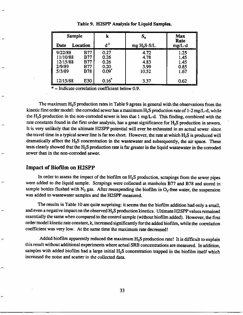
Table 9. H2SPP Analysis for Liquid Samples .

* = Indicate correlation coefficient below 0.9 .

The maximum H2S production rates in Table 9 agrees in general with the observations from thekinetic first order model : the corroded sewer has a maximum H2S production rate of 1-2 mg/L-d, whilethe H2S production in the non-corroded sewer is less that 1 mg/L-d. This finding, combined with therate constants found in the first order analysis, has a great significance for H 2S production in sewers .It is very unlikely that the ultimate H2SPP potential will ever be exhausted in an actual sewer sincethe travel time in a typical sewer line is far too short . However, the rate at which H 2S is produced willdramatically affect the H2S concentration in the wastewater and subsequently, the air space. Thesetests clearly showed that the H2S production rate is far greater in the liquid wastewater in the corrodedsewer than in the non-corroded sewer .

Impact of Biofilm on H2SPP

In order to assess the impact of the biofilm on H 2S production, scrapings from the sewer pipeswere added to the liquid sample . Scrapings were collected at manholes B77 and B78 and stored insample bottles flushed with N 2 gas. After resuspending the biofilm in 02-free water, the suspensionwas added to wastewater samples and the H2SPP measured .

The results in Table 10 are quite surprising : it seems that the biofilm addition had only a small,and even a negative impact on the observed H 2S production kinetics . UltimateH2SPP values remainedessentially the same when compared to the control sample (without biofilm added) . However, the firstorder model kinetic rate constant, k, increased significantly for the added biofilm, while the correlationcoefficient was very low. At the same time the maximum rate decreased!

Added biofilm apparently reduced the maximum H2S production rate! It is difficult to explainthis result without additional experiments where actual SRB concentrations are measured . In addition,samples with added biofilm had a large initial H 2S concentration trapped in the biofilm itself whichincreased the noise and scatter in the collected data.

33

Sample

Date Location

k

d- '

S•

mg H2S-S/L

MaxRatemg/L-d

9/22/88

B77 0.27 4.72 1.2511/10/88

B77 0.26 4.78 1.4512/15/88

B77 0.26 4.83 1.452/9/89

B77 0.20 3.99 0.855/3/89

B78 0.09* 10.52 1 .67

12/15/88

E30 0.16* 3.37 0.62

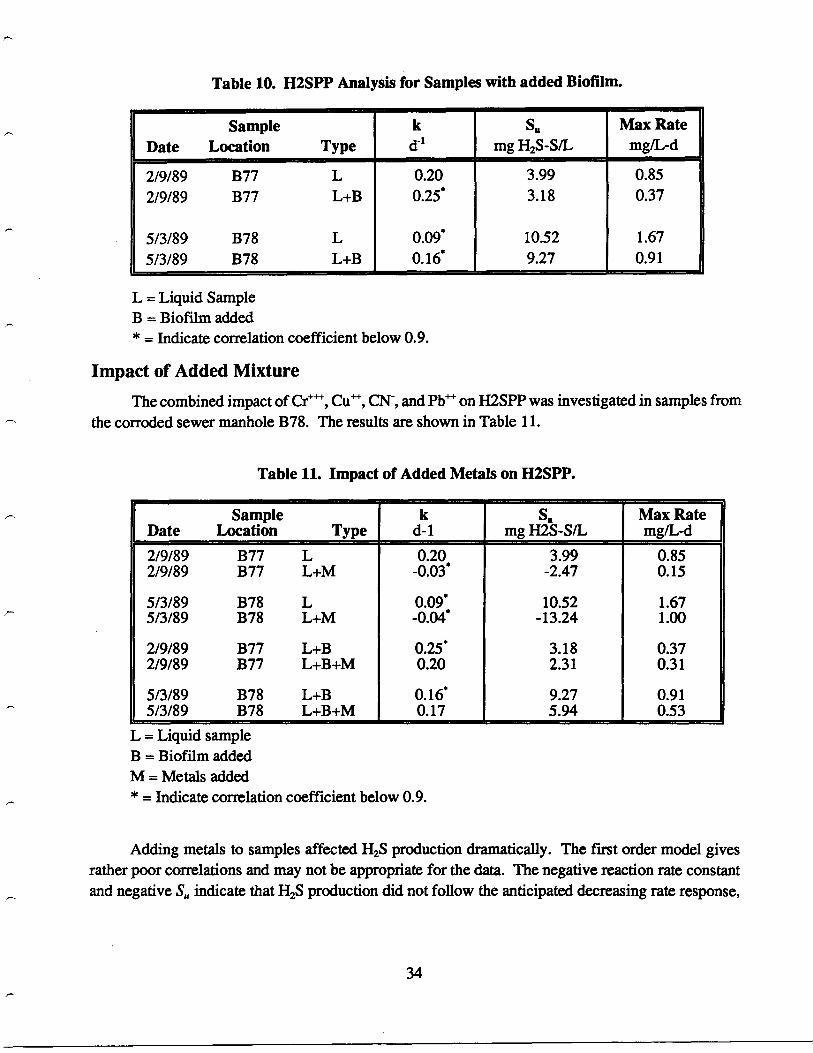
Table 10. H2SPP Analysis for Samples with added Biofilm .

L = Liquid SampleB = Biofilm added* = Indicate correlation coefficient below 0 .9 .

Impact of Added MixtureThe combined impact of Cr, Cu', CN - , and Pb' on H2SPP was investigated in samples from

the corroded sewer manhole B78 . The results are shown in Table 11 .

Table 11. Impact of Added Metals on H2SPP.

L = Liquid sampleB = Biofilm addedM = Metals added* = Indicate correlation coefficient below 0 .9.

Adding metals to samples affected H2S production dramatically . The first order model givesrather poor correlations and may not be appropriate for the data. The negative reaction rate constantand negative Su indicate that H2S production did not follow the anticipated decreasing rate response,

34

SampleDate

Location

Typek

d-1S•

mg H2S-S/LMax Ratemg/L-d

2/9/89

B77

L 0.20 3.99 0.852/9/89

B77

L+M -0.03* -2.47 0.15

5/3/89

B78

L 0.09' 10.52 1 .675/3/89

B78

L+M -0.04* -13.24 1.00

2/9/89

B77

L+B 0.25* 3.18 0.372/9/89

B77

L+B+M 0.20 2.31 0.31

5/3/89

B78

L+B 0.16* 9.27 0.915/3/89

B78

L+B+M 0.17 5.94 0.53

SampleDate Location

Typekd''

S•mg H2S-S/L

Max Ratemg/L-d

2/9/89

B77

L 0.20 3.99 0.852/9/89

B77

L+B 0.25* 3.18 0.37

5/3/89

B78

L 0.09* 10.52 1.675/3/89

B78

L+B 0.16* 9.27 0.91

but rather an increasing rate, meaning that the model was a poor fit for the observed data . Both liquidsamples with metals showed this poor correlation. The increased H2S production rate is indicative ofthe first part of the classic S shaped curve .

The maximum H2S production rates give results that are much easier to interpret . Adding themix to samples reduced the maximum H2S production rate significantly . Liquid H2S production ratesdecreased between 40 and 80% and biofilm rates between 16 and 42% after adding the mix. Thisreduction is quite significant since the actual H2S production rate is of great importance in the sewermodel to determine the amount of H2S generated during the travel time to the treatment plant .

Metals can reduce the H2SPP in two ways : by direct inhibition of SRB, or by chemical reactionswith dissolved sulfides . This study did not attempt to determine the exact mode of action . A moreencompassing study needs to be conducted to determine the mechanism in which metals reduce H 2Sproduction rates . In the tests performed so far, the H 2S production proceeded at an increased rate,following the first stage of the traditional S shaped curve . This may indicate either an initial inhibition,that is overcome in later stages, or an initial reaction between H 2S and added metals to form precipitates,thus preventing H2S evolution from the liquid .

SIGNIFICANCE OF RESULTS

This report describes a kinetic model for H 2S production in sewers. The model includes bacterialsulfur reduction in the wastewater and biofilm, and the impact of chemical reactions and mass transferon the evolution of H2S from the liquid into the air space . A proper understanding of the H2S productionkinetics in the sewer is of great importance .

H2S production in wastewater samples follows a typical S-shape curve . Initially H2S evolutionis slow due to low SRB numbers, potential inhibitors (such as DO or NOD, or reactions between liquidcompounds and dissolved sulfides . As time progresses, the rate increases to reach a maximum, followedby a reduction in rate possible due to a substrate limitation, end-product inhibition, or some otherunknown factor.

The. maximum H2S production rate and lag time before H 2S evolution occurs is of great sig-nificance in predicting and describing H2S evolution from wastewater in a typical sewer . If the lagperiod is significant, the wastewater may reach the treatment plant before conditions in the pipe isconducive to H2S production. Or, if the H2S production rate is reduced significantly by additives, theH2S concentration in the liquid may be sufficiently reduced to prevent H 2S evolution from the liquidin significant quantities .

The ultimate significance of the reaction rate kinetics and impact of metals or waste activatedsludge on H2S production rates can be evaluated using the proposed kinetic sewer model . However,in order to use the model, reaction rates that account for added inhibitors, DO, and added aerobicorganisms must be determined .

35

Waste activated sludge added to the sewer at upstream treatment plants may have a significantimpact on H2S production. The added waste activated sludge contain large quantities of active aerobicbacteria, which will rapidly consume the available oxygen to generate favorable conditions in the sewerfor H2S production.

Results so far showed that metals have a significant impact on H2S production . Both the firstorder reaction rate constant and the maximum H2S production rate decrease significantly when metalsare added to the solution. In addition, it seems that there is an increase in the lag period before H 2Sproduction occur. Both these factors will reduce the H 2S production in a flowing sewer, where onlya limited amount of time is available for H 2S production and evolution.

NOMENCLATURE

Saturation concentration of species x in the liquid phase, in equilibrium with the gasphase concentration, g/m3 (or mg/L). C* is calculated using Henry's Law .

CBOD

= BOD concentration in wastewater, mg/L as S

C,,

= Combined sulfide concentration, mg/L as S

Cd,,

= Dissolved sulfide concentration, mg/L as S

Cfx

= Concentration of species x in the film, mg/L

CSO4

= Sulfate concentration, mg/L as S

C~,

= Total sulfide concentration, mg/L as S

Cx

= Concentration of species x, mg/L

Dx

= Diffusion coefficient of species x into the biofilm, m2/h

E

= Potential of the cell, volt

E°

= Standard potential of the cell, volt

F

= Faradys constant, 23,062 cal/volt-eq

Hx

= Henry's law coefficient for species x, mg/L-atm

km,x

= Maximum reaction rate, mg/L-h

(KLa)x = Mass transfer coefficient for species x into the liquid, m/h

K,

= Half saturation coefficient, mg/L .

Mr

= Effective sulfide flux coefficient for sulfide generated in slime, m/h

M2

= Sulfide production rate coefficient

Nx

= Flux of species x into the liquid phase, g/m2-h

36

C*x

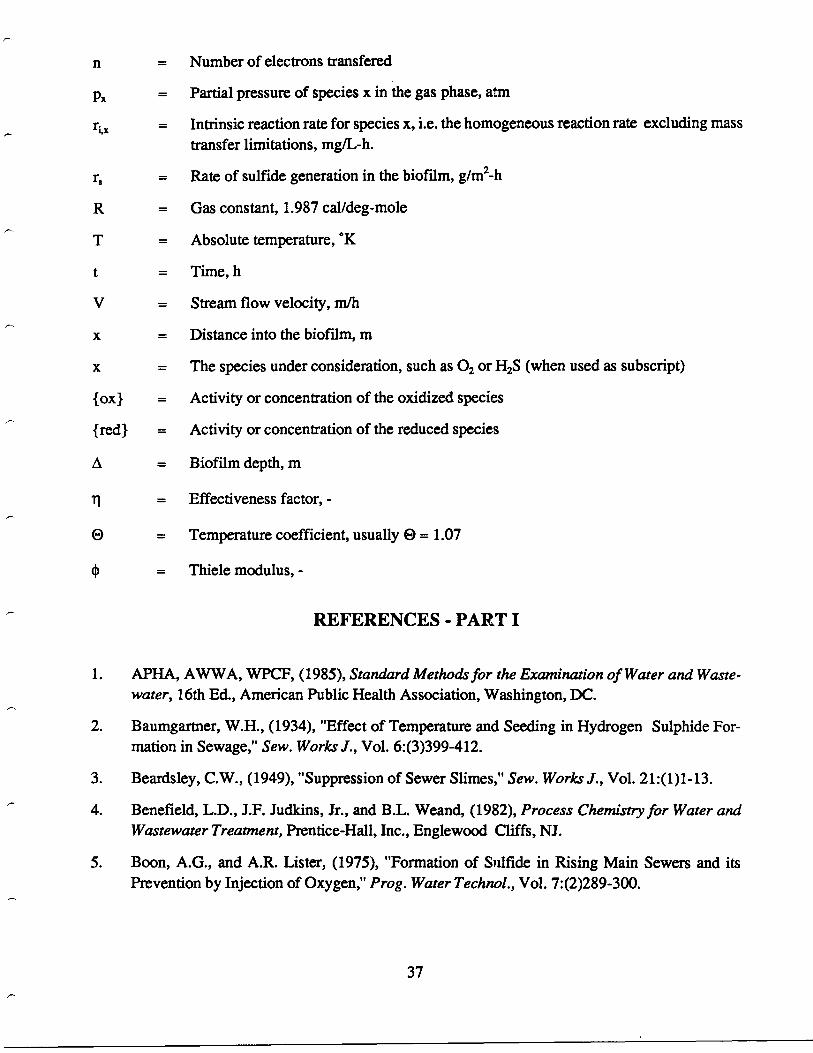
n

= Number of electrons transfered

p x

= Partial pressure of species x in the gas phase, atm

r;, x

= Intrinsic reaction rate for species x, i .e. the homogeneous reaction rate excluding masstransfer limitations, mg/L-h .

r,

= Rate of sulfide generation in the biofilm, g/m 2-h

R

= Gas constant, 1 .987 cal/deg-mole

T

= Absolute temperature, °K

t

= Time, h

V

= Stream flow velocity, m/h

x

= Distance into the biofilm, m

x

= The species under consideration, such as 02 or H2S (when used as subscript)

{ox}

= Activity or concentration of the oxidized species

{red}

= Activity or concentration of the reduced species

0

= Biofilm depth, m

11

= Effectiveness factor, -

O

= Temperature coefficient, usually O = 1 .07

0

= Thiele modulus, -

REFERENCES - PART I

1 . APHA, AWWA, WPCF, (1985), Standard Methods for the Examination of Water and Waste-water, 16th Ed., American Public Health Association, Washington, DC .

2 .

Baumgartner, W.H., (1934), "Effect of Temperature and Seeding in Hydrogen Sulphide For-mation in Sewage," Sew. Works J., Vol. 6:(3)399-412 .

3 .

Beardsley, C.W., (1949), "Suppression of Sewer Slimes," Sew. Works J., Vol. 21:(1)1-13 .

4.

Benefield, L .D., J.F. Judkins, Jr., and B .L. Weand, (1982), Process Chemistry for Water andWastewater Treatment, Prentice-Hall, Inc., Englewood Cliffs, NJ .

5 .

Boon, A.G., and A.R. Lister, (1975), "Formation of Sulfide in Rising Main Sewers and itsPrevention by Injection of Oxygen," Prog. Water Technol., Vol. 7:(2)289-300.

37

6.

Borland, J., (1987), "Oxygenation of Gravity Sewers to Control Odours," IMIESA, Vol.12:(10)7-13 .

7 .

Bowlus, F.D., and A.P. Banta, "Control of Sewage Condition by Chlorination," Water WorksSew., Vol . 79:(11)369-374.

8 . Chen, K.Y., and J.C. Morris, (1970), "Oxidation of Aqueous Sulfide by 0 2. 1 . General Char-acteristics and Catalytic Influences," Presented at the5thlnternational WaterPollution ResearchConference, Paper 111-32, July-August 1970.

9 .

Chen,K.Y., and J.C. Morris, (1972), "Kinetics of Oxidation of Aqueous Sulfide by 0 2," Environ.Sci. Technol., Vol . 6:(6)529-537 .

10. Dahod, S.K., (1983), "Redox Potential as a Better Substitute for Dissolved Oxygen in Fer-mentation Process Control," Biotechnol. Bioengrg., Vol . XXIV:2123-2125 .

11 . Davy, W.J., (1950), "Influence of Velocity on Sulfide Generation in Sewers," Sew. Indus .Wastes, Vol. 22:(9)1132-1137.

12 . El-Rayes, H.H., (1988), "Biochemical Control of Sulfide Production in Wastewater CollectionSystems," Ph.D. Thesis, New Mexico State University, Las Cruces, NM, December 1988 .

13 . Eliassen, R., A.N. Heller, and G . Kisch, (1949), "The Effect of Chlorinated Hydrocarbons onHydrogen Sulfide Production," Sew. Work J., Vol . 21 :(3)457-474.

14. Harremoes, P., (1978), "Biofilm Kinetics," in Water Pollution Microbiology, R. Mitchell (Eds),John Wiley and Sons, Vol. 2:71-109.

15 . Hauser, J., and G .A. Holder, (1988), "Apparatus for Assessing Sulfide Generation Rates fromSewer Slimes," J. Environ. Engrg., Am. Soc. Civ. Eng., Vol. 114:(4)977-981 .

16 . Heukelekian, H., (1948), "Some Bacteriological Aspect;, of Hydrogen Sulfide Production fromSewage," Sew. Works J., Vol. 20:(3)490-498 .

17 . Holder, G.A., (1986), "Prediction of Sulfide Build-Up in Filled Sanitary Sewers," J. Environ .Engrg., Am. Soc. Civ. Eng., Vol . 112:(2)199-210 .

18 . Holder, G.A., G. Vaughan, and W . Drew, (1985), "Kinetic Studies of the MicrobiologicalConversion of Sulphate to Hydrogen Sulfide and their Relevance to Sulphide Generation withinSewers," Water Sci. Technol., Vol. 17:(2/3)183-196 .

19 . Jameel, P., "The Use of Ferrous Chloride to Control Dissolved Sulfides in Interceptor Sewers,"J. Water Pollut. Control Fed., Vol. 62:(2)230-236.

20. Kienow, K.E., R.D. Pomeroy, and K.K. Kienow, (1982), "Prediction of Sulfide Buildup inSanitary Sewers," J. Environ. Engrg., Am. Soc. Civ. Eng ., Vol. 108:(EE5)941-956.

21 . Meyer, W.J ., (1980), "Case Study of Prediction of Sulfid Generation and Corrosion in Sewers,"J. Water Pollut. Control Fed., Vol. 52:(11)2666-2674 .

38

22. Moeller, T ., and R. O'Connor, (1972), Ions in Aqueous Systems, McGraw-Hill Book Company,New York.

23. Neethling, J.B., (1988), "The Role of Diffusion in the Activated Sludge Process," Environ .Technol. Letters, Vol. 9:1187-1200 .

24 . Nielsen, P .H., and T. Hvitved-Jacobsen, (1988), "Effect of Sulfate and Organic Matter onHydrogen Sulfide Formation in Biofilms of Filled Sanitary Sewers," J. Water Pollut. ControlFed., Vol . 60:(5)627-634.

25 . Parker, C.D., (1951), "Mechanics of Corrosion of Concrete Sewers by Hydrogen Sulfide," Sew .Indus. Wastes, Vol . 23:(12)1477-1485 .

26. Pomeroy, R., (1945), "The Pros and Cons of Sewer Ventilation," Sew. Works J., Vol .17:(2)203-206 .

27 . Pomeroy, R., and F.D. Bowlus, (1946), "Progress Report on Sulfide Control Research," Sew .WorksJ., Vol. 18:(4)597-640 .

28 . Pomeroy, R.D., and J.D. Parkhurst, (1977), "The Forecasting of Sulfide Buildup Rates inSewers," Prog. Water Technol ., Vol. 9:621-628 .

29 . Pomeroy,R.D., (1956), "Control of Hydrogen Sulfide Generation in Sewers," Water Sew. Works,133-136 .

30. Postgate, J.R., (1963), "Versatile Medium for the Enumeration of Sulfate-Reducing Bacteria,"Appl. Microbiol., Vol. 11 :265-267.

31 . Postgate, J.R., (1984), The Sulfate Reducing Bacteria (2nd Ed.), Cambridge University Press,Cambridge .

32. Rudolfs, W ., and W.H. Baumgartner, (1932), "Studies on Hydrogen Sulfide Formation inSewage," Ind. Engrg. Chem ., Vol. 24:(10)1152-1154.

33. Snoeyink, V.L., and D. Jenkins, (1980), Water Chemistry, John Wiley and Sons, New York,NY.

34. Stumm, W., and J.J. Morgan, (1970), Aquatic Chemistry, Wiley-Interscience, New York.

35 . Thistlethwayte, D.K.B., (1972), The Control of Sulphides in Sewerage Systems, Ann ArborScience, MI.

36 . Thomas, Jr., H.A., (1950), "Graphical Determination of BOD Curve Constants," Water Sew .Works, Vol. 97:123 .

37. US EPA, (1985), Design Manual. Odor and Corrosion Control in Sanitary Sewerage Systemsand Treatment Plants, United States Environmental Protection Agency publicationEPA/625/1-85/018, Office of Research and Development, Cincinnati, OH, October 1985 .

39

38. Van Durme, G.P., and K .J. Berkenpas, (1989), "Comparing Sulfide Control Products," Oper-ations Forum, Vol. 6:(2)12-19.

40

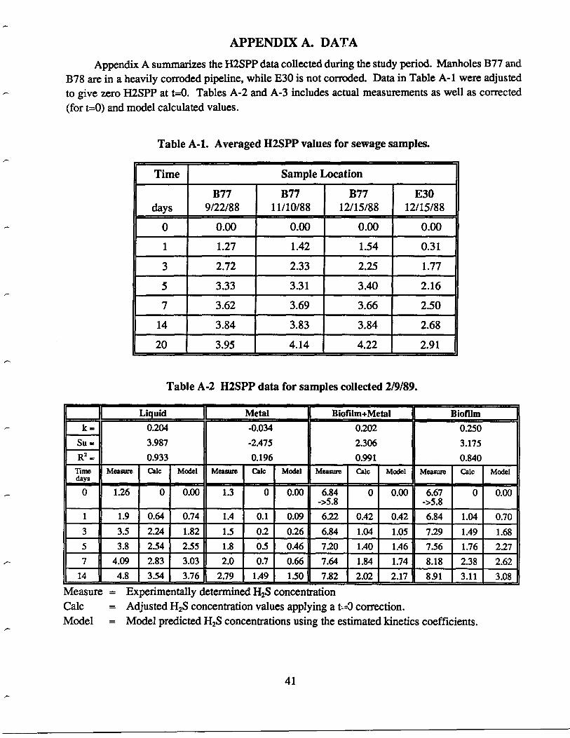
APPENDIX A. DATAAppendix A summarizes the H2SPP data collected during the study period . Manholes B77 and

B78 are in a heavily corroded pipeline, while E30 is not corroded . Data in Table A-1 were adjustedto give zero H2SPP at t=0. Tables A-2 and A-3 includes actual measurements as well as corrected(for t=0) and model calculated values .

Table A-1. Averaged H2SPP values for sewage samples.

Table A-2 H2SPP data for samples collected 2/9/89 .

Measure = Experimentally determined H 2S concentrationCalc

= Adjusted H2S concentration values applying a t==0 correction .Model = Model predicted H2S concentrations using the estimated kinetics coefficients .

41

Liquid Metal Biofilm+Metal Biofilmk = 0.204

3.9870.933

-0.034-2.4750.196

0.2022.3060.991

0.2503.1750.840

Su =R2 =Timedays

Measure Calc Model

/

Measure Calc Model Measure Calc Model Measure Calc Model

0 1.26 0 0.00 1.3 0 0.00 6.84 0 0.00 6.67 0 0.00->5.8 ->5.8

1 1 .9 0.64 0.74 1 .4 0.1 0.09 6.22 0.42 0.42 6.84 1 .04 0.703 3.5 2.24 1.82 1 .5 0.2 0.26 6.84 1.04 1 .05 7.29 1.49 1 .685 3.8 2.54 2.55 1 .8 0.5 0.46 7.20 1.40 1.46 7.56 1 .76 2.277 4.09 2.83 3.03 2.0 0.7 0.66 7.64 1.84 1.74 8.18 2.38 2.62

14 4.8 3 .54 3.76 2.79 1 .49 1 .50 7.82 2.02 2.17 8.91 3 .11 3 .08

Time Sample Location

B77 B77 B77 E30days 9/22/88 11/10/88 12/15/88 12/15/88

0 0.00 0.00 0.00 0.00

1 1 .27 1.42 1.54 0.31

3 2.72 2.33 2.25 1 .77

5 3.33 3.31 3.40 2.16

7 3.62 3.69 3.66 2.50

14 3.84 3.83 3.84 2.68

20 3.95 4.14 4.22 2.91

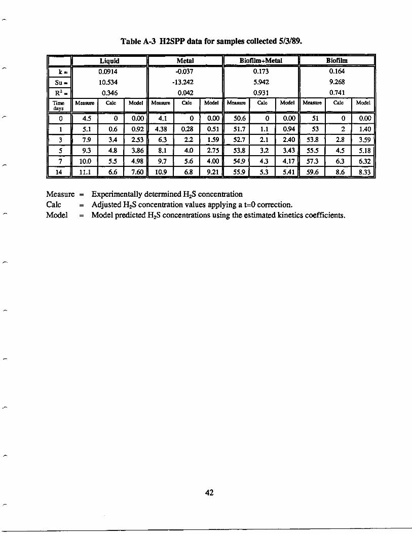
Table A-3 H2SPP data for samples collected 5/3/89 .

Measure = Experimentally determined H 2S concentrationCalc

= Adjusted H2S concentration values applying a t=0 correction .Model = Model predicted H2S concentrations using the estimated kinetics coefficients .

42

L

Liquid Metal Bioflm+Metal Biofilm

10.091410.5340.346

-0.037-13.2420.042

0.1735.9420.931

0.1649.2680.741

Su -R2 =Timedays

Measure Calc Model Measure CaIc Model Measure Calc Model Measure Calc Model

0 4.5 0 0.00 4.1 0 0.00 50.6 0 0.00 51 0 0.001 5.1 0.6 0.92 . 4.38 0.28 0.51 51 .7 1 .1 0.94 53 2 1.40

2.53 ` 6.33 7.9 3 .4 22 1 .59 52.7 2.1 2.40 53 .8 2.8 3.595 9.3 4.8 3.86 8.1 4.0 2.75 53.8 3.2 3.43 55.5 4.5 5.187 10.0 5.5 4.98 9.7 5.6 4.00 54 .9 4.3 4.17 57.3 6.3 6.32

14 11 .1 6.6 7.60 10.9 6.8 9.21 55.9 5.3 5.41 59.6 8.6 8.33

PART II. SULFATE-REDUCING BACTERIA INCONCRETE SEWER PIPES`

In sewage effluent contained by concrete sewer pipes during transport to the waste treatmentfacility, sulfate-reducing bacteria (SRB) are responsible for production of the sewer gas sulfide andare a major factor in microbial concrete corrosion . Although SRB's are strictly anaerobic, they areubiquitous and are found even in aerobic environments . They show considerable adaptability in termsof temperature and salinity, tolerating temperatures from below -5 ° to 75 °C, pH value ranging from5 to 9.5 and salinity up to 18% (Jorgensen, 1977) . They may also be oxygen toleranct ; Desulfobacterpostgatei and pesulfovibrio species are known to be oxygen-resistant (Hardy, 1981 ; Cypionka, 1985) .Cypionka et al, 1985, reported that the following SRB 's, Desulfovibrio vulaaris. Desulfovibrio baarsii,Desulfobacter postgatei. Desulfobulbus propionicus.Desulfococcus multivorans. Desulfonemalimicola. Desulfosarcina variabilis and Desulforomonas acetoxidans, used thiosulfate or sulfur aselectron acceptors and exhibited oxygen-dependent growth in sulfate- and sulfur-free medium . Theyform thiosulfate or sulfur by continuously regenerating them in a cycling process from sulfide byautoxidation. Our studies are focused on the SRB and their physiology in both pure and mixed culturesystems under strictly anaerobic conditions . We developed a reliable medium and culture conditionsfor enumerating SRB's by MPN analysis of mixed culture inocula taken from natural samples . Thisculture protocol was also assessed by using axenic cultures of laboratory strains of SRB's . Becauseof the superiority of this medium, we have used it for isolation of three strains of SRB 's from culturesoriginally inoculated with biofilm from a corroding sewer pipe and have begun their characterization .As model systems for the inhibition of sulfate reduction of SRB, we established stable enrichmentcultures using lactate as a single sulfidogenic substrate . These enrichment cultures were used asmicrocosms to simulate the sewer pipe environment for sulfide-inhibition experiments . We summarizehere our experimental studies on the isolation of SRB, evaluation of media and experiments oninhibition of sulfate reduction .

MATERIALS AND METHODSMedia and Enumeration Techniques : We reviewed the composition of various published

media most commonly used in the isolation and growth of SRB's . Postgate's Medium B and Pfennig'senrichment medium were selected for comparison with alpha medium which was developed in ourown laboratory. Table 1 compares the composition of the three media . Most-Probable-Number (MPN)of the biofilm sample obtained from site #B78 were evaluated in these media and the results werecompared (Table 3). The medium which gave the highest bacterial count was used in the subsequentexperiments. Throughout these studies we employed the techniques of Hungate (Hungate, 1969) asmodified by Bryant (Bryant, 1972) for the culture of strictly anaerobic microorganisms .

*R.A. Mah

43

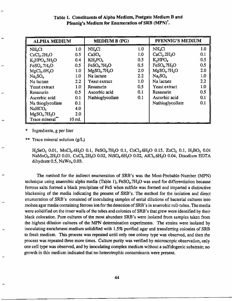
Table 1. Constituents of Alpha Medium, Postgate Medium B andPfennig's Medium for Enumeration of SRB (MPN)~ .

* Ingredients, g per liter

** Trace mineral solution (g/L)

H2Se03 0.01, MnC12.4H20 0.1, FeSO4.7H20 0.1, CoC12.6H20 0.15, ZnC12 0.1, H3B03 0.01NaMoO4.2H20 0.01, CuC12.2H20 0.02, NiSO4.6H20 0.02, A1C13.6H20 0.04, Disodium EDTAdihydrate 0.5, NaWo 4 0.03 .

The method for the indirect enumeration of SRB's was the Most-Probable-Number (MPN)technique using anaerobic alpha media (Table 1), FeSO 4.7H20 was used for differentiation becauseferrous salts formed a black precipitate of FeS when sulfide was formed and imparted a distinctiveblackening of the media indicating the present of SRB's . The method for the isolation and directenumeration of SRB's consisted of inoculating samples of serial dilutions of bacterial cultures intomolten agar media containing ferrous ion for the detection of SRB 's in anaerobic roll-tubes . The mediawere solidified on the inner walls of the tubes and colonies of SRB 's that grew were identified by theirblack coloration . Pure cultures of the most abundant SRB's were isolated from samples taken fromthe highest dilution cultures of the MPN determination experiments . The strains were isolated byinoculating enrichment medium solidified with 1 .5% purified agar and transferring colonies of SRBto fresh medium. This process was repeated until only one colony type was observed, and then theprocess was repeated three more times . Culture purity was verified by microscopic observation, onlyone cell type was observed, and by inoculating complex medium without a sulfidogenic substrate ; nogrowth in this medium indicated that no heterotrophic contaminants were present .

44

ALPHA MEDIUM MEDIUM B (PG) PFENNIG'S MEDIUM

NH4C1 1.0 NH4C1 1.0 NH4C1 1.0CaC12.2H20 0.5 CaSO4 1 .0 CaC12.2H20 0.1K2HPO4.3H20 0.4 KH2P04 0.5 K2HPO4 0.5FeSO4.7H20 0.5 FeSO4.7H20 0.5 FeSO4.7H20 0.5MgC12.6H20 1.0 MgS04.7H20 2.0 MgSO4.7H20 2.0Na2SO4 1.0 Na lactate 2.2 Na2SO4 1.0Na lactate 2.2 Yeast extract 1 .0 Na lactate 2.2Yeast extract 1.0 Resazurin 0.5 Yeast extract 1 .0Resazurin 0.5 Ascorbic acid 0.1 Resazurin 0.5Ascorbic acid 0.1 Nathioglycollate 0.1 Ascorbic acid 0.1Na thioglycollate 0.1 Nathioglycollate 0.1NaHCO3 4.0MgS04.7H20 2.0Trace mineral` 10 ml .

Enumeration of SRB in The Concrete Sewers : The numbers of SRB's in the samples ofsewage and biofilm were determined by the MPN technique . Sewer and biofilm samples were collectedat Compton, CA on 25 August 1988, from manhole #B78, a site where concrete corrosion is verysevere, and manhole #E30 which is considered a clean, non-corroding pipe segment . The bottlescontaining water samples were filled and capped so no air was entrapped and anaerobic conditionswere maintained. The biofilm samples were scraped from the sides of the pipe with the bottle mouthand the headspace of the bottles was flushed with pure nitrogen gas to exclude air . Biofilm sampleswere diluted with the culture medium for inoculation of MPN experiments .

Inhibition of Sulfate Reduction Experiments : To test for inhibition of sulfate reduction byoxyanion group VI elements, chromate, tungstate, selenate and molybdate, we added the oxyanionsat varying concentrations to freshly inoculated cultures of two SRB enrichment cultures . The SRBenrichments were initiated by inoculating samples of sewage (Sample #1) and biofilm (Sample #2)from site #B78 severe concrete corrosion . The enrichment cultures were grown as batch cultures withlactate as substrate ; a 2.5% inoculum was transferred routinely to fresh medium every 7-10 days sinceDecember 1988 .

The enrichment alpha medium (Table 2) was modified from the MPN alpha medium by replacingFeSO4.7H20 and MgSO4.7H20 with Na2SO4 as a sole sulfate source ; CaC12.2H20 was decreased inconcentration to 0 .1 g/L in order to avoid black precipitation of FeS and to reduce interference fromcalcium salts while measuring the bacterial growth and sulfide concentration . Na2S, a reducing agent,was also used in the enrichment medium to reduce the redox potential low enough to initiate growthof SRB's.

Table 2. Constituents of Alpha Medium for InhibitorExperiments (Enrichment Medium).

45

Ingredients g/L

NH4C1 1 .0CaC12.2H20 0.1MgC12.6H20 1.0K2HPO4 0.4Na2SO4 1 .4NaHC03 4.0Na lactate 2.2Yeast extract 0.5Resazurin 0.5Na2S.9H20 0.24Trace mineral solution 10.0 ml.

An untreated control culture inoculated with the same sample was incubated for the same periodof time and analyzed for sulfide production . In every case, the control sample metabolized all of theavailable sulfate and converted it to sulfide as measured by the methylene blue method (Triiper andSchlegel, 1964) . The oxyanionic inhibitors were prepared anaerobically, the pH was adjusted to 7 .0and sterilized by autoclaving before use . A 5% inoculum of a late logarithmically grown culture wasused; the estimated number of cells in this innoculum was 1-1 .6 x 108 organisms/ml. All cultures wereincubated at 37 ©C for a minimum of 7-10 days and analyzed for sulfide production periodically .

RESULTS AND DISCUSSION

The mineral composition of the alpha medium was based on a standard mixture of inorganicsalts normally employed for culture of other anaerobic bacteria in our laboratory . It differed signifi-cantly from the medium of Postgate and Pfennig by addition of a trace mineral solution and by theaddition of sufficient quantities of bicarbonate-CO 2 to maintain the buffering capacity of the mediumat pH 7.0 • 0 .2. These differences, and the use of the Hungate technique, most likely accounted forthe improved reproducibility of our method and the more consistent replication of data compared tomedia used by other researchers (Grossman, 1953; Postgate,1959 ; Iverson, 1966) . Our MPN experi-ments using alpha medium yielded two to three fold higher counts than the other media (ExperimentI, Table 3). In subsequent experiments, comparing alpha medium and Postgate's medium B using thesame anaerobic techniques, there was no difference statistically between these two media . However,alpha medium always yielded higher counts on the average with a more consistency in the replica(Experiment II, Table 3) .

Table 3. Comparing MPN Results of Biofilm Sample Site #B78 inAlpha Medium, Postgate Medium B and Pfennig's Medium.

46

Type of medium MPN ml-'

Experiment I:Alpha 3.4 x 108Postgate's B 2.6 x 108Pfenning's 1 .0 x 108

Experiment II:Alpha #1 6.0 x 107

#2 1 .4 x 108#3 1.4 x 108

average = 1.1 • 0.4 x 108

Postgate's #1 6.0 x 107#2 6.0 x 107#3 1 .6 x 108

average = 0.9 • 0.5 x 108

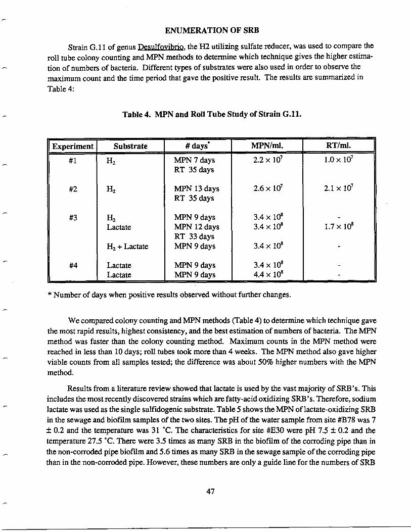
ENUMERATION OF SRB

Strain G. 11 of genus pesulfovibrio, the H2 utilizing sulfate reducer, was used to compare theroll tube colony counting and MPN methods to determine which technique gives the higher estima-tion of numbers of bacteria . Different types of substrates were also used in order to observe themaximum count and the time period that gave the positive result. The results are summarized inTable 4 :

Table 4. MPN and Roll Tube Study of Strain G.11 .

* Number of days when positive results observed without further changes .

We compared colony counting and MPN methods (Table 4) to determine which technique gavethe most rapid results, highest consistency, and the best estimation of numbers of bacteria . The MPNmethod was faster than the colony counting method . Maximum counts in the MPN method werereached in less than 10 days ; roll tubes took more than 4 weeks . The MPN method also gave higherviable counts from all samples tested ; the difference was about 50% higher numbers with the MPNmethod.

Results from a literature review showed that lactate is used by the vast majority of SRB's . Thisincludes the most recently discovered strains which are fatty-acid oxidizing SRB's . Therefore, sodiumlactate was used as the single sulfidogenic substrate . Table 5 shows the MPN of lactate-oxidizing SRBin the sewage and biofilm samples of the two sites . The pH of the water sample from site #B78 was 7• 0.2 and the temperature was 31 ©C . The characteristics for site #E30 were pH 7.5 • 0.2 and thetemperature 27.5 ©C. There were 3.5 times as many SRB in the biofilm of the corroding pipe than inthe non-corroded pipe biofilm and 5.6 times as many SRB in the sewage sample of the corroding pipethan in the non-corroded pipe . However, these numbers are only a guide line for the numbers of SRB

47

# 1 H2 MPN 7 daysRT 35 days

2.2 x 10 1 .0 x 10'

#2 H2 MPN 13 daysRT 35 days

2.6 x 10' 2.1 x 10'

#3 H2 MPN 9 days 3.4 x 108 -Lactate MPN 12 days

RT 33 days3.4 x 108 1.7 x 108

H2 + Lactate MPN 9 days 3.4 x 108 -

#4 Lactate MPN 9 days 3.4 x 108 -Lactate MPN 9 days 4.4 x 108 -

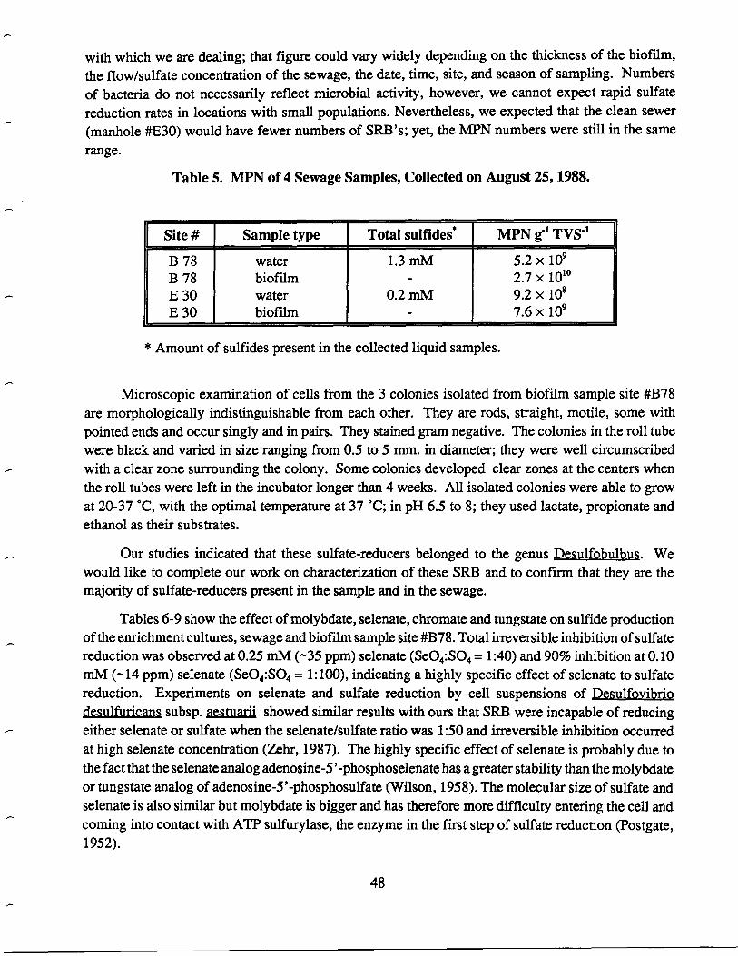
with which we are dealing ; that figure could vary widely depending on the thickness of the biofilm,the flow/sulfate concentration of the sewage, the date, time, site, and season of sampling . Numbersof bacteria do not necessarily reflect microbial activity, however, we cannot expect rapid sulfatereduction rates in locations with small populations . Nevertheless, we expected that the clean sewer(manhole #E30) would have fewer numbers of SRB's; yet, the MPN numbers were still in the samerange .

Table 5. MPN of 4 Sewage Samples, Collected on August 25, 1988 .

* Amount of sulfides present in the collected liquid samples .

Microscopic examination of cells from the 3 colonies isolated from biofilm sample site #B78are morphologically indistinguishable from each other . They are rods, straight, motile, some withpointed ends and occur singly and in pairs. They stained gram negative. The colonies in the roll tubewere black and varied in size ranging from 0.5 to 5 mm. in diameter; they were well circumscribedwith a clear zone surrounding the colony. Some colonies developed clear zones at the centers whenthe roll tubes were left in the incubator longer than 4 weeks . All isolated colonies were able to growat 20-37 ©C, with the optimal temperature at 37 ©C; in pH 6.5 to 8; they used lactate, propionate andethanol as their substrates .

Our studies indicated that these sulfate-reducers belonged to the genus Desulfobulbus . Wewould like to complete our work on characterization of these SRB and to confirm that they are themajority of sulfate-reducers present in the sample and in the sewage .

Tables 6-9 show the effect of molybdate, selenate, chromate and tungstate on sulfide productionof the enrichment cultures, sewage and biofilm sample site #B78 . Total irreversible inhibition of sulfatereduction was observed at 0.25 mM (-35 ppm) selenate (Se04:SO4 =1:40) and 90% inhibition at 0 .10mM (-14 ppm) selenate (Se0 4:SO4 =1 : 100), indicating a highly specific effect of selenate to sulfatereduction . Experiments on selenate and sulfate reduction by cell suspensions of Desulfovibriodesulfuricans subsp . aestuarii, showed similar results with ours that SRB were incapable of reducingeither selenate or sulfate when the selenate/sulfate ratio was 1 :50 and irreversible inhibition occurredat high selenate concentration (Zehr, 1987) . The highly specific effect of selenate is probably due tothe fact that the selenate analog adenosine-5'-phosphoselenate has a greater stability than the molybdateor tungstate analog of adenosine-5'-phosphosulfate (Wilson, 1958) . The molecular size of sulfate andselenate is also similar but molybdate is bigger and has therefore more difficulty entering the cell andcoming into contact with ATP sulfurylase, the enzyme in the first step of sulfate reduction (Postgate,1952) .

48

I Site # Sample type Total sulfides' MPN g'1 TVS-'

B 78 water 1 .3 mM 5.2 x 109B 78 biofilm - 2.7 x 10 10

E 30 water 0.2 mM 9.2 x 108E 30 biofilm - 7.6 x 109

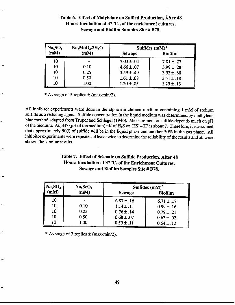
* Average of 5 replica • (max-min/2) .

All inhibitor experiments were done in the alpha enrichment medium containing 1 mM of sodiumsulfide as a reducing agent . Sulfide concentration in the liquid medium was determined by methyleneblue method adapted from Truper and Schlegel (1946). Measurement of sulfide depends much on pHof the medium. At pH7 (pH of the medium) pK of H2S a HS" + H+ is about 7 . Therefore, it is assumedthat approximately 50% of sulfide will be in the liquid phase and another 50% in the gas phase . Allinhibitor experiments were repeated at least twice to determine the reliability of the results and all wereshown the similar results .

Table 7. Effect of Selenate on Sulfide Production, After 48Hours Incubation at 37 ©C, of the Enrichment Cultures,

Sewage and Biofilm Samples Site # B78 .

* Average of 3 replica • (max-min/2) .

49

Table 6. Effect of Molybdate on Sulfied Production, After 48Hours Incubation at 37 ©C., of the enrichment cultures,

Sewage and Biofilm Samples Site # B78 .

Na2SO4(mm)

Na2MoO4.2H20(mm)

Sulfides (mM)*Sewage

Bioflm10 - 7.03 • .04 7.01• .2710 0.10 4.66• .07 3.99• .2810 0.25 3.59 • .49 3.92 • .3810 0.50 1 .61• .08 3.51• .1810 1 .00 1 .20 • .05 1 .23 • .13

Na2SO4(mm)

Na2Se04(mm)

Sulfides (mM)*Sewage

Biofilm10 - 6.87• .16 6.71• .1710 0.10 1 .14• .11 0.99• .1610 0.25 0.76• .14 0.79• .2110 0.50 0.68 • .07 0.63 • .0210 1 .00 0.59• .11 0.64• .12

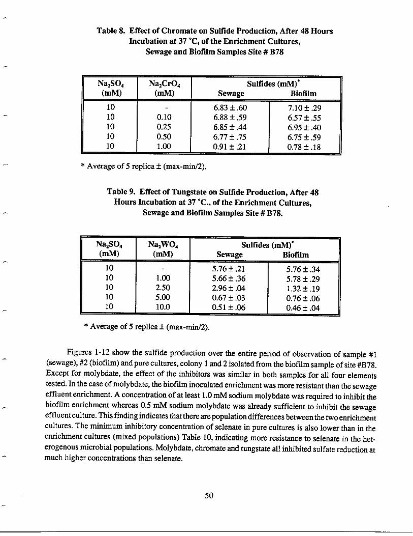
Table 8. Effect of Chromate on Sulfide Production, After 48 HoursIncubation at 37 ©C, of the Enrichment Cultures,

Sewage and Bioflm Samples Site # B78

* Average of 5 replica • (max-min/2) .

Table 9. Effect of Tungstate on Sulfide Production, After 48Hours Incubation at 37 ©C., of the Enrichment Cultures,

Sewage and Biofilm Samples Site # B78 .

* Average of 5 replica • (max-min/2) .

Figures 1-12 show the sulfide production over the entire period of observation of sample #1(sewage), #2 (biofilm) and pure cultures, colony 1 and 2 isolated from the biofilm sample of site #B78 .Except for molybdate, the effect of the inhibitors was similar in both samples for all four elementstested. In the case of molybdate, the biofilm inoculated enrichment was more resistant than the sewageeffluent enrichment. A concentration of at least 1 .0 mM sodium molybdate was required to inhibit thebiofilm enrichment whereas 0 .5 mM sodium molybdate was already sufficient to inhibit the sewageeffluent culture . This finding indicates that there are population differences between the two enrichmentcultures . The minimum inhibitory concentration of selenate in pure cultures is also lower than in theenrichment cultures (mixed populations) Table 10, indicating more resistance to selenate in the het-erogenous microbial populations . Molybdate, chromate and tungstate all inhibited sulfate reduction atmuch higher concentrations than selenate .

50

Na2SO4(MM)

Na2CrO4(MM)

Sulfides (mM) *Sewage

Biofilm

10 - 6.83• .60 7.10• .2910 0.10 6.88 • .59 6.57 • .5510 0.25 6.85 • .44 6.95 • .4010 0.50 6.77 •35 6.75 • .5910 1 .00 0.91• .21 0.78• .18

Na2SO4(MM)

Na2WO4(MM)

Sulfides mM)*Sewage

Bioflm10 - 5.76 • .21 5.76• .3410 1 .00 5.66 •36 5.78 • .2910 2.50 2.96• .04 1.32• .1910 5 .00 0.67 • .03 0.76 • .0610 10.0 0.51 • .06 0.46• .04

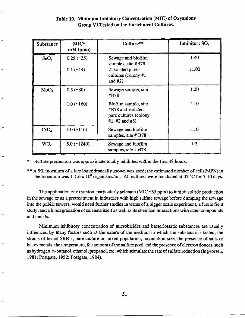
Table 10. Minimum Inhibitory Concentration (MIC) of OxyanionsGroup VI Tested on the Enrichment Cultures .

* Sulfide production was approximate totally inhibited within the first 48 hours .

** A 5% inoculum of a late logarithmically grown was used ; the estimated number of cells(MPN) inthe inoculum was 1-1 .6 x 108 organisms/ml. All cultures were incubated at 37 ©C for 7-10 days .

The application of oxyanion, particularly selenate (NUC -35 ppm) to inhibit sulfide productionin the sewage or as a pretreatment in industries with high sulfate sewage before dumping the sewageinto the public sewers, would need further studies in terms of a bigger scale experiment, a future fieldstudy, and a biodegradation of selenate itself as well as its chemical interactions with other compoundsand metals .

Minimum inhibitory concentration of microbicides and bacteriostatic substances are usuallyinfluenced by many factors such as the nature of the medium in which the substance is tested, thestrains of tested SRB's, pure culture or mixed population, inoculation size, the presence of salts orheavy metals, the temperature, the amount of the sulfate pool and the presence of electron donors, suchas hydrogen, n-butanol, ethanol, propanol, etc . which stimulate the rate of sulfate reduction (Ingvorsen,1981 ; Postgate, 1952 ; Postgate, 1984) .

51

Substance MIC*MM (ppm)

Culture** Inhibitor: SO4

Se04 0.25(-35)

0.1(-14)

Sewage and biofilmsamples, site #B782 Isolated pure -cultures (colony #1and #2)

1 :40

1 :100

MoO4 0.5(-80)

1 .0(-160)

Sewage sample, site#B78

Biofilm sample, site#B78 and isolatedpure cultures (colony#1, #2 and #3)

1 :20

1 :10

Cr04 1 .0(-116) Sewage and biofilmsamples, site # B78

1 :10

W04 5.0(-1240) Sewage and biofilmsamples, site # B78

1 :2

The recent isolation of two new species of Desulfovibrio capable of utilizing higher fatty acidsup to eighteen carbons (Widdel, 1981) and the description (Pfennig, 1981 ; Widdel, 1982) of five newgenera of SRB, Desulfobacter, Desulfosarcina, Desulfonema, Desulfobulbus, and Desulfococcus thatare morphologically and nutritionally diverse has completely destroyed the concept that the SRB area small and highly specialized group with a limited metabolic versatility . This physiological diversityof SRB's was observed in our pure cultures isolated from the biofilm sample, site #B78 .

Therefore, the control of sulfide production and concrete corrosion may be specific to each localewith the majority of resident SRB's enriched by local selective factor of pH, temperature, substrateavailability, presence or absence of heavy metals, in situ combinations of oxyanions, etc .

PROPOSAL TO LA COUNTY ON SRBOur previous studies indicate that sulfate-reducing bacteria belonging to the genus Desulfobulbus

rather than to the more commonly occurring Desulfovibrio predominate in all sewage samples thusfar examined. This ecological study needs further verification on additional samples, and we proposeto do further viable counts on freshly sampled sewage to establish this finding . This verification isimportant in the design for inhibition of sulfide production experiments . The genus Desulfobulbus iscapable of using propionate as well as lactate as electron donor and carbon source . They also are ableto use other inorganic compounds such as nitrate as electron donors . In other words they can use muchwider variety of compounds as electron donors and carbon sources . In addition to examining thenumerical importance of Desulfobulbus,, we also propose to study the effect of the following sulfate-reducing inhibitors on both pure cultures of the most numerous sulfate-reducer isolated from the sewagesamples and on natural mixed cultures of unenriched sewage samples :

1 . Arquad 16 50%* (N,N,N-Trimethyl-l-hexadecanaminium chloride)

2. Arquad S 50%* (Trimethylsoya alkyl quaternary ammonium chlorides)

3 . Arquad 2C 75%* (Dicoco alkyldimethyl quaternary ammonium chlorides)

4 . Hibitane (Chlorhexidine acetate)

* Arquads are quaternary ammonia compounds, widely used in the textile industry as an antistaticagent, in pesticide/herbicide formulations, in cosmetic formulations as an ingredient in hair con-ditioners, toiletries and fragrances, etc .

These compounds were selected from a list of sulfate-inhibitors compiled by Postgate (1984)from publications reported by several research groups . The studies were performed on pure culturesof Desulfovibrio or Desulfotomaculum or on mixed, impure cultures . We selected the above com-pounds because of their low minimum inhibitory concentrations (ranging from 0 .1 to 50 °g/ml) andthe wide use of the Arquad compounds .

52

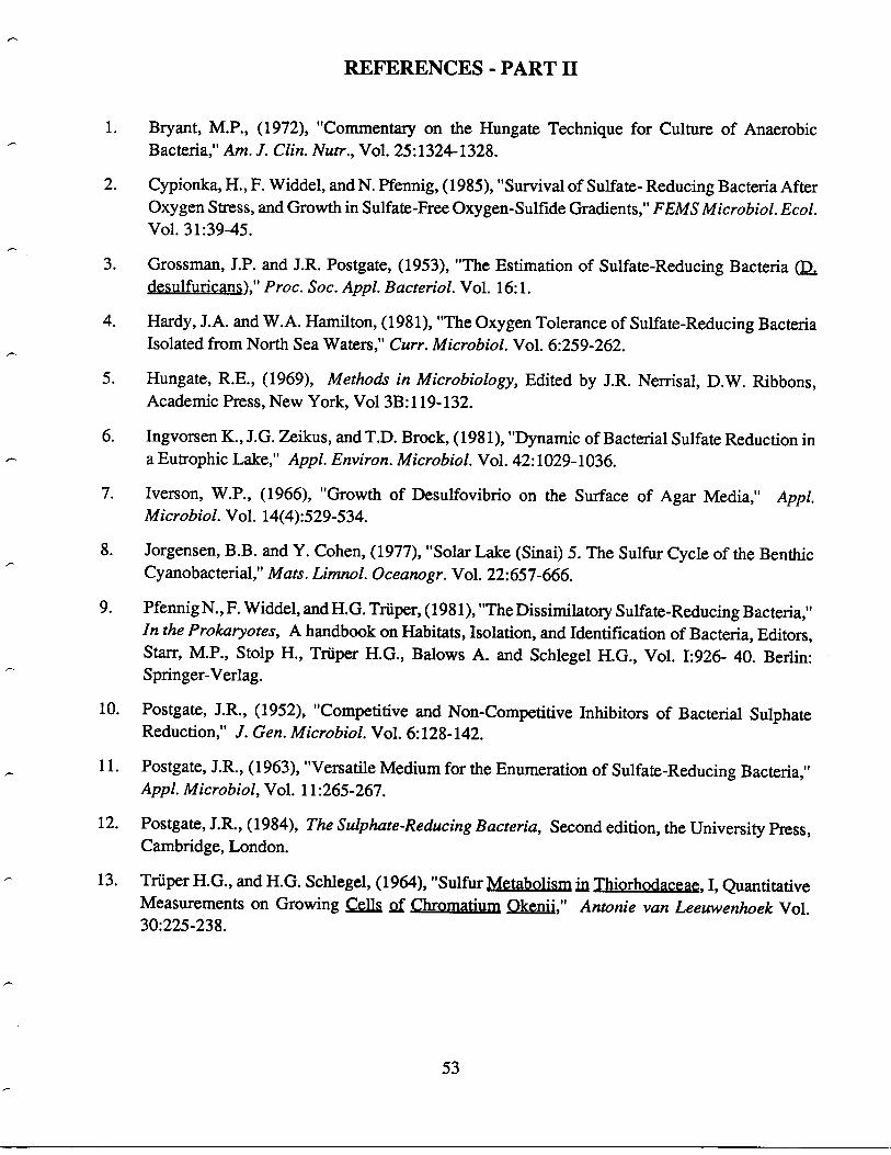
REFERENCES - PART II

1 .

Bryant, M.P., (1972), "Commentary on the Hungate Technique for Culture of AnaerobicBacteria," Am. J. Clin. Nutr ., Vol. 25:1324-1328 .

2. Cypionka, H ., F. Widdel, and N . Pfennig, (1985), "Survival of Sulfate- Reducing Bacteria AfterOxygen Stress, and Growth in Sulfate-Free Oxygen-Sulfide Gradients," FEMS Microbiol . Ecol.Vol. 31 :39-45 .

3 .

Grossman, J.P. and J.R. Postgate, (1953), "The Estimation of Sulfate-Reducing Bacteria (D,desulfuricans)," Proc. Soc. Appl. Bacteriol . Vol. 16:1 .

4 .

Hardy, J.A. and W.A. Hamilton, (1981), "The Oxygen Tolerance of Sulfate-Reducing BacteriaIsolated from North Sea Waters," Curr. Microbiol . Vol. 6:259-262.

5 .

Hungate, R.E., (1969), Methods in Microbiology, Edited by J.R. Nerrisal, D.W. Ribbons,Academic Press, New York, Vol 3B :119-132 .

6 .

Ingvorsen K ., J.G. Zeikus, and T.D. Brock, (1981), "Dynamic of Bacterial Sulfate Reduction ina Eutrophic Lake," Appl. Environ. Microbiol . Vol. 42:1029-1036.

7 .

Iverson, W.P., (1966), "Growth of Desulfovibrio on the Surface of Agar Media," Appl.Microbiol . Vol. 14(4):529-534 .

8 .

Jorgensen, B .B. and Y. Cohen, (1977), "Solar Lake (Sinai) 5 . The Sulfur Cycle of the BenthicCyanobacterial," Mats. Limnol. Oceanogr. Vol. 22 :657-666.

9. Pfennig N., F. Widdel, and H.G. Truper, (1981), "The Dissimilatory Sulfate-Reducing Bacteria,"In the Prokaryotes, A handbook on Habitats, Isolation, and Identification of Bacteria, Editors,Starr, M .P., Stolp H., Triiper H .G., Balows A. and Schlegel H.G., Vol. 1:926- 40 . Berlin:Springer-Verlag .

10. Postgate, J.R., (1952), "Competitive and Non-Competitive Inhibitors of Bacterial SulphateReduction," J. Gen. Microbiol . Vol. 6:128-142 .

11 . Postgate, J .R., (1963), "Versatile Medium for the Enumeration of Sulfate-Reducing Bacteria,"Appl. Microbiol, Vol. 11 :265-267 .

12. Postgate, J .R., (1984), The Sulphate-Reducing Bacteria, Second edition, the University Press,Cambridge, London.

13. Truper H.G., and H.G. Schlegel, (1964), "Sulfur Metabolism in Thiorhodaceae, I, QuantitativeMeasurements on Growing Cells f Chromatium Okenii," Antonie van Leeuwenhoek Vol.30:225-238 .

53

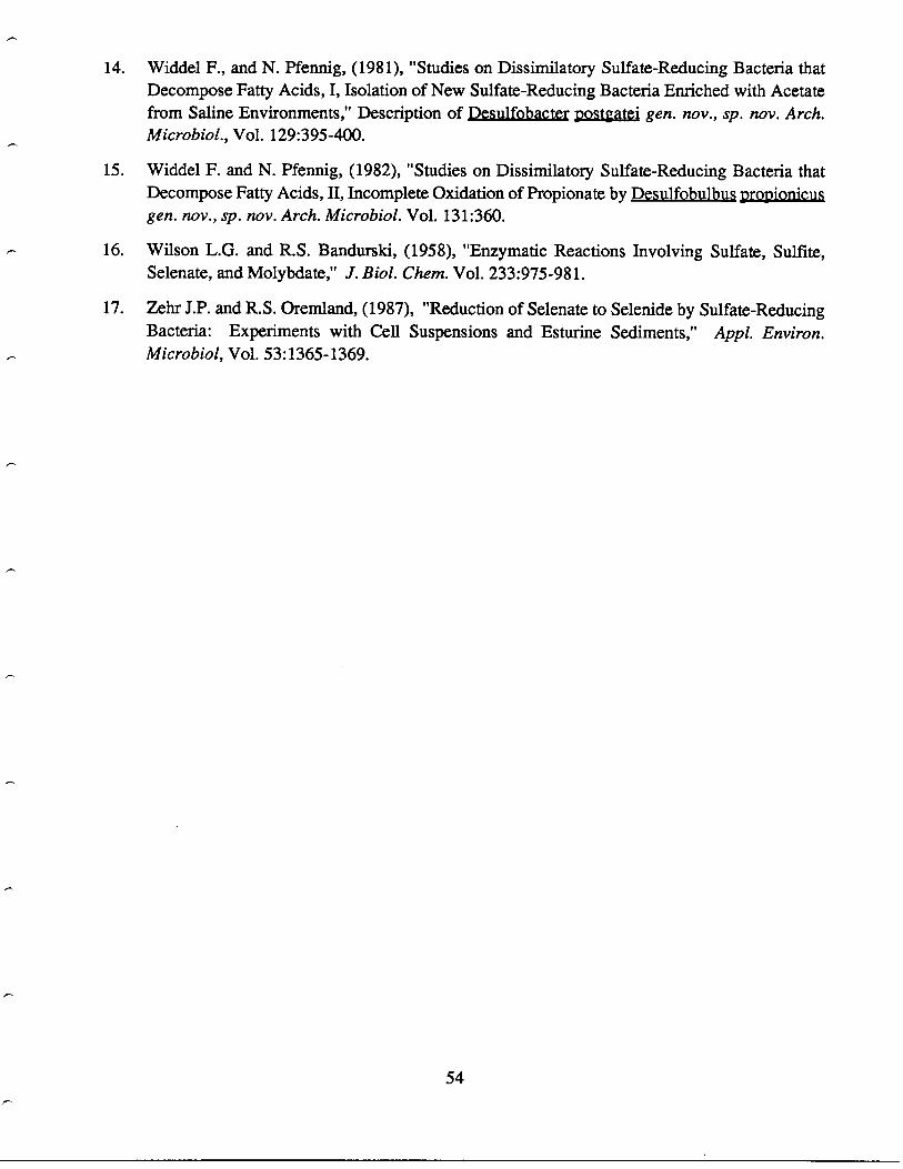
14 . Widdel F., and N. Pfennig, (1981), "Studies on Dissimilatory Sulfate-Reducing Bacteria thatDecompose Fatty Acids, I, Isolation of New Sulfate-Reducing Bacteria Enriched with Acetatefrom Saline Environments," Description of pesulfobacter posteatei gen. nov., sp. nov. Arch .Microbiol ., Vol. 129 :395-400 .

15 . Widdel F. and N. Pfennig, (1982), "Studies on Dissimilatory Sulfate-Reducing Bacteria thatDecompose Fatty Acids, II, Incomplete Oxidation of Propionate by Desulfobulbus propionicusgen. nov., sp. nov. Arch. Microbiol. Vol . 131 :360.

16. Wilson L.G. and R.S . Bandurski, (1958), "Enzymatic Reactions Involving Sulfate, Sulfite,Selenate, and Molybdate," J. Biol. Chem. Vol . 233:975-98 1 .

17 . Zehr J.P. and R.S . Oremland, (1987), "Reduction of Selenate to Selenide by Sulfate-ReducingBacteria: Experiments with Cell Suspensions and Esturine Sediments," Appl. Environ .Microbiol, Vol. 53:1365-1369 .

54

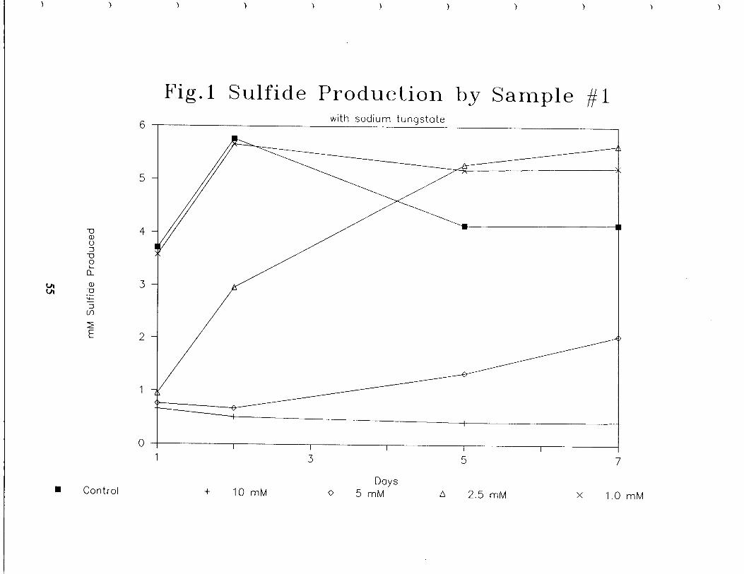
Fig .1 Sulfide Production by Sample #1with sodium tungstate

+

10 mm

3 5

Days0

5mM

o

2 .5mM

7

X

1 .0 m M

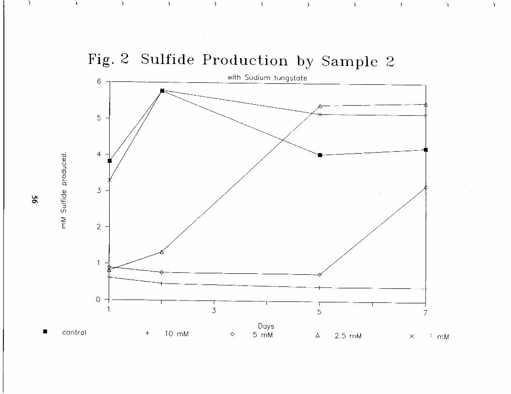
Fig . 2 Sulfide Production by Sample 2with Sodium tungstate

+

10 mmDays

O

5 mM 0

2 .5 m M

E

a

Fig . 3 Sulfide Production by Sample # 1with Sodium molybdate .

0

+

1 mm 0

0 .50 mMDays

4

L

0.25 mM x

0.10 mm

E

0

Fig .4 Sulfide Production by Sample #2with Sodium molybdate .

+

1 .0 mmDays

0

0 .50 mM

4

0

0 .25 mM x

0.10 mm

+

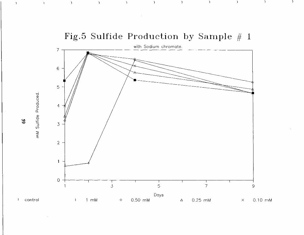
1 mm

Fig.5 Sulfide Production by Sample 1/ 1with Sodium chromate .

0

0 .50 mMDays

0

0.25 mM x

0.10 mm

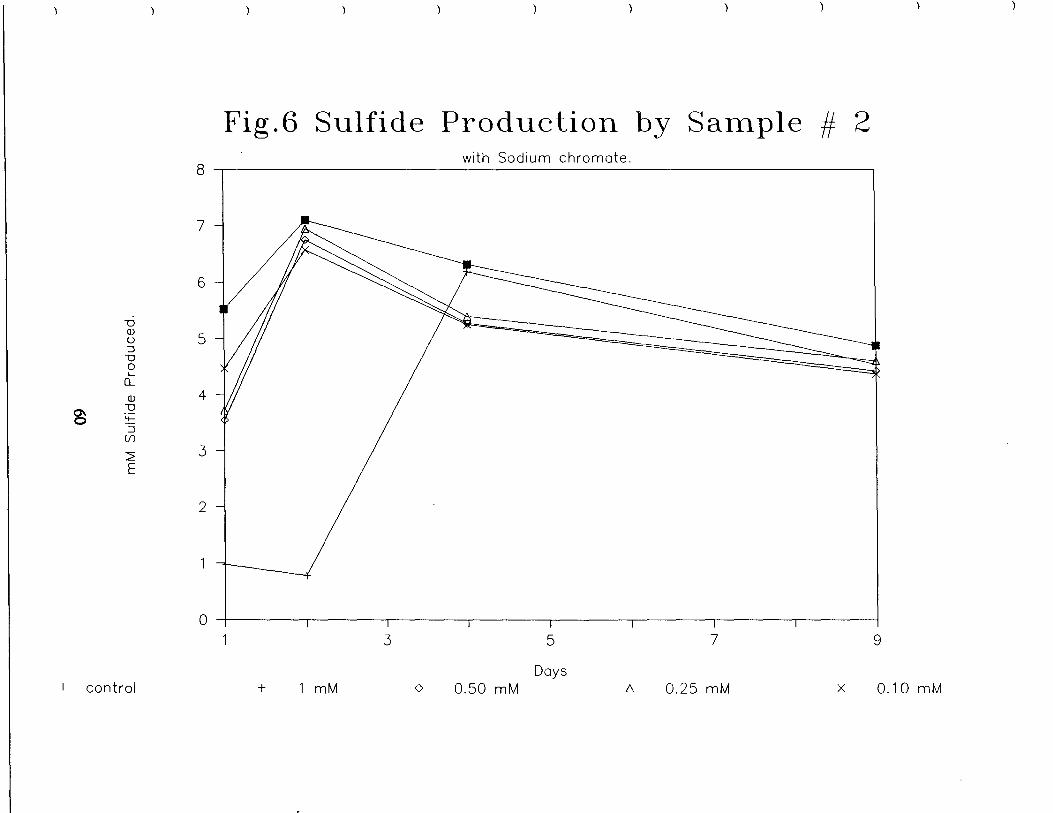
I

control

Fig.6 Sulfide Production by Sample # 2

1

+

1 mm

3

with Sodium chromate .

0

0 .50 mM

5

Days

7

A

0 .25 mM

9

x

0.10 mm

8

7

6

050

0L -n~,

4

:2

3E

2

1

0

0\

L-n

:2

3E

8

7

6

2

0

Fig.7 Sulfide Production by Sample 1/ 1with Sodium selenote .

I

I

0

2

4

6

x

Daysi control

+

1 mm

o

0.50 mM

o

0.25 mM

x

0.10 mm

8

7

6

12

3E

2

0

Fig .8 Sulfide Production by Sample # 2with Sodium selenate .

0i

2

+

1 mm

0

0.50 mMDays

4

0

0.25 mM

i6

6e

i

x

0.10 mm

8

7

6

4-

2

1

0

with Sodium molybdate .

1

1

2

3

)

Figure9 :Sulfide Production of Colony /11

80

1

8

10

Daysƒ

control

+

1 mm

o

2.5 mM

o

5 mM

x

10 mm

'Da)U

0V -a-

ƒ

control

FigurelO :Sulfide Production of Colony#2with Sodium molybdate .

1

+

1 mm

3

Days .0

2 .5 m M

5

0 5 mM

7

x

10 mm

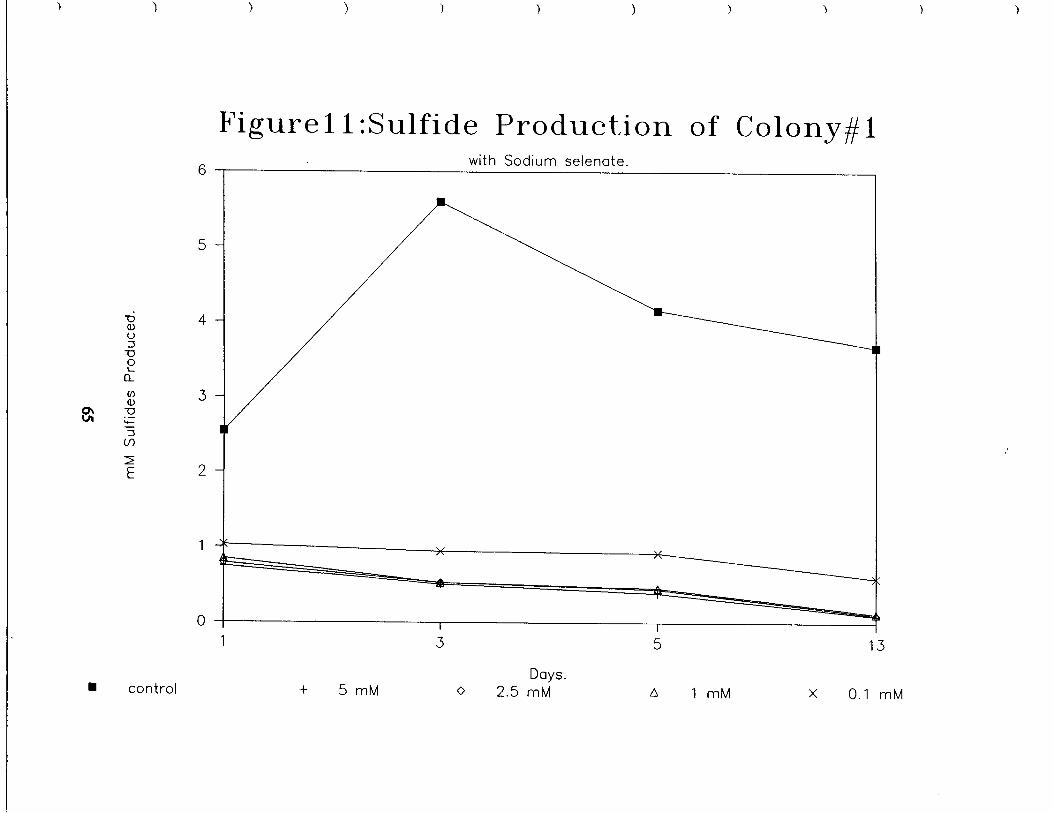
a

dN

3D

1

0

6

5

ƒ

control

Figure ll :Sulfide Production of Colony#1with Sodium selenate .

1

+ 5 mM

3

Days .0

2 .5 m M

5

A

1 mm

13

x

0.1 m M

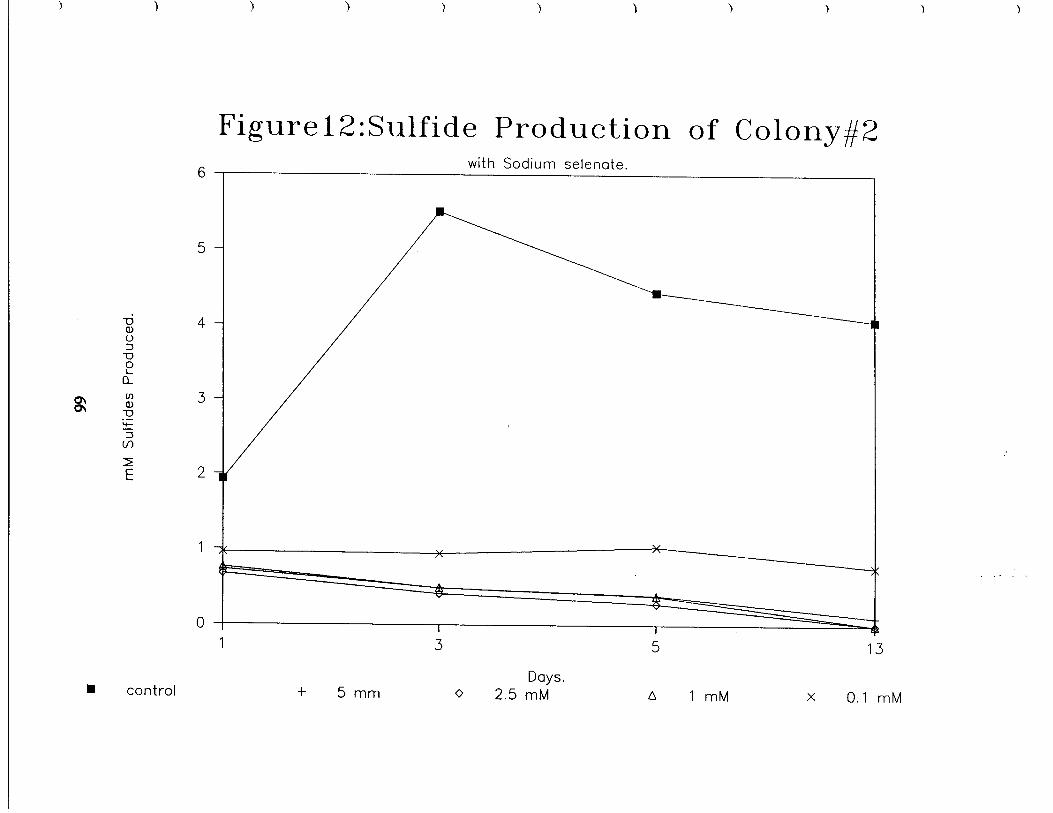
ƒ

control

Figure l2 :Sulfide Production of Colony#2 with Sodium se lenate .

+ 5 mmDays .

0

2 .5 m M

5

0

1 mm

13

x

0.1 m M

PART III. ESTIMATION VOLATILIZATION OF REDUCEDSULFUR COMPOUNDS

The release of volatile reduced sulfur containing compounds (VS Cs) from untreatedwastewaters and during wastewater treatment is a known side effect of wastewater collection andtreatment. In the past interest was focused primarily on H 2S emissions and its malodorous quali-ties and high toxicity, which caused health and safety problems for operation and maintenancepersonnel. It was observed, however, as early as 1900 (Olmstead and Hamlin) that concretesewers showed signs of rapid corrosion . This phenomenon was most frequently observed inwastewater collection systems in warm climates . Investigators assumed that H 2S, formed bydecomposition of organic material or by sulfate reduction in the wastewater, escaped into thesewer atmosphere where it was oxidized to sulfuric acid .

The occurrence of concrete corrosion in wastewater collection systems in colder climatesin the late 70s prompted further research. The high sulfur content in detergents and increasedprotein content of wastewaters might enhance production of volatile sulfur compounds (VS Cs)in wastewaters during transport (Sand and Bock, 1984 ; Milde et al., 1983) .

It has been known since the early 70s (Okita, 1969 ; Thistlethwayte and Goleb, 1972) thatH2S is not the only VSC in the atmosphere or in wastewater. Thistlethwayte found that in addi-tion to H2S, methylmercaptan (MMC) and dimethylsulfide (DMS) were the predominant sulfurcontaining species in sewer gas, and that wastewater composition strongly affects the type andconcentration of VSCs. It is conceivable that these organic volatile sulfur compounds (OVSCs)have contributed to the total sulfur deposition on the pipe walls and may be responsible for atleast part of the H2SO4 formation that finally leads to corrosion .

In order to assess the contribution of OVSCs to concrete corrosion in wastewater collec-tion systems two sets of questions must be answered :

1 . What are the sources of the VSCs in sewer gases? What are their respective rates of pro-duction, mass transfer rates to the gas phase, and mechanisms for deposition on pipewalls? How do environmental conditions affect those rates?

2.

Are all of these VSCs easily oxidized in sewer gas or on the pipe walls to form H 2SO4?

This report will exclusively address the first set of questions, with a strong emphasis onmass transfer; however, it should be indicated that in the process of performing this researchseveral contradictory references addressing the second set of questions were found, and thatexperimental evidence seems contradictory . Sand (1987) reports that a mixed culture of

67

thiobacilli that were found on pipe walls were not able to oxidize methylmercaptan, whereasSivela and Sundmann (1974) found that a thiobacillus strain was able to oxidize MMC, DMS,and dimethyldisulfide (DMDS) in a culture medium . A more definitive answer as to the condi-tions where OVSCs might be oxidized to H2SO4 on pipe walls is essential in order to assess theirsignificance for corrosion .

This report addresses the literature on the occurrence of VCS's in sewage and its sourceand reviews mass transfer theory and develops the theoretical basis for a numerically basedmodel to calculate stripping of VSCs from wastewater collection systems . It also describes theselected procedures and the specifics of the computer model .

The remainder of this report is divided into four sections . Section 1 addresses the litera-ture on the occurrence of VSCs in sewages and its source . Section 2 reviews mass transfertheory and develops the theoretical basis for a numerically based model to calculate stripping ofVSCs from wastewater collection systems . Section 3 describes the selected procedures and Sec-tion 4 describes the specifics of the computer model .

OCCURRENCE AND SOURCES OF VSCs

Monitoring Results for VSCs

Various measurements of the concentration of the major VSCs in sewer gas, or in thevicinity of sewers, suggest that the most predominant species are H2S, MMC, DMS, and DMDS .Some of these compound's physical and chemical properties are listed in Table 1 . Our reviewsuggests that there is no simple or known relationship describing their relative abundance .Thistlethwayte and Goleb (1972) found mostly H 2S in sewer gas above mixed municipal sewageat a site in Sydney, Australia. Concentrations were 0 .2 to 10 ppmv. OVSCs totaled 10 to 50ppbv with most of it being MMC with some DMS . The authors concluded, that for this particu-lar site, the OVSCs/H2S ratio ranged from 1 :50 to 1 :100. Other gas samples collected fromwastewater treatment systems carrying discharges from a large kraft pulp mill, and from otherindustries including the manufacture of dairy products, showed H 2S and mercaptan levels ofhundreds of ppmv. A wastewater collection system near Melbourne, containing highly septicmixed municipal sewage, showed high H 2S levels and an OVSCs/H2S ratio ranging from 1 :5 to1 :10 .

68

Koenig et al., (1980) report only DMS and dimethyltrisulfide in sewer gas . After inten-sive purging of municipal sewage at 80©C they found a third OVSC, dimethyltetrasulfide. Theoccurrence of dimethyltrisulfide and dimenthyltetrasulfide as predominant OVSCs has not beenreported by any other researchers. Their findings might have been influenced by the purgingprocedure.

Monitoring data of ambient air for VSCs in the vicinity of several sewage transport andtreatment facilities in Finland were provided by Kangas et al. (1986). They found, somewhatcontradictory to Thistlethwayte, that around pumping stations, where ambient air is probablymost similar to sewer gas, MMC and DMS were as abundant as H2S . Concentrations for allthree species averaged about 50 ppbv . Around screens and aeration basins MMC was in generalmore prevalent than H2S. DMDS could not be detected in any of the samples.

Comparison of the two studies and other references suggests that the relative significanceof each of the VSCs or OVSCs in sewer gas depends on the specific source of a wastewater andthe conditions of its transport . The use of different analytical procedures may have contributedto the variation in the results .

Sources of VSC in Wastewater Treatment Systems

Several sources with specifically high emissions of OVSCs were found in the literature .Okita (1969) reports MMC (5 .6 ppbv) and DMS (3 .5 ppbv) to be predominant over H2S (0.66ppbv) in ambient air in an oil refinery in Japan . Ambient air in a pulp mill contained 57 ppbv ofMMC and 2.8 ppbv of DMS, with no H2S being reported. Pulp mills are an important source ofVSCs in air, as well as in wastewater, and are frequently cited in the literature . Sivela and Sund-mann (1974) mention that "condensates of sulfate cellulose mills contain high concentrations ofH2S, MMC, DMS and DMDS . These toxic and malodorous waste products are formed from themethoxy groups of lignin in the pulping process ."

Oil refinery wastewater can be another source of VSCs in wastewater collection systems .Jenkins et al. (1980) report that various mercaptans were found in the wastewater from refineriesand headspace gas. He also reports that MMC is produced by the decomposition of heavierorganosulfur compounds, such as hexylmercaptan, during activated sludge treatment .

A very important source of sulfur in wastewater are the sulfur containing amino acidsmethionine and cysteine . They can occur in high concentrations in wastewater from food pro-cessing industries (meat, fish, dairy) and are common in domestic wastewater . Pohl and Bock(1983) report that MMC, DMS, and DMDS were produced by the bacterial degradation ofmethionine . H2S was not reported. Cultures of E.coli, Proteus vulgaris, Pseudomonas

69

aeruginosa, Clostridium tetani have been shown to produce methylmercaptan but not H 2S frommethionine (Salsbury and Merricks, 1975) . Alternatively from cysteine they can produce H 2S.cysteine (Salsbury and Merricks, 1975) . Relative rates of production for each of the VSCs willdepend strongly on the presence of the appropriate strains of bacteria which can utilize themunder the prevailing oxygen and substrate concentrations .

The prevailing opinion among environmental engineers is that the major production ofH2S in wastewater results because of the use of SO4 as an electron acceptor in anoxic or anaero-bic environments. Domestic water use generally increases the sulfate content of wastewaters by15-30 mg/l (Metcalf and Eddy, 1979) . Sea water intrusions into groundwater supplies can alsoresult in increased sulfate levels. Industrial discharge of SO4 from neutralization processes is yetanother sulfate source.

Finally, anionic surfactants with a sulfonate group as the hydrophilic component are nor-mally used in laundry detergents, with linear-alkyl-sulfonates (LAS) being the major representa-tives. No information on typical sulfonate concentrations in sewage and on the fate of the sulfurwere found. However, their use in large quantities suggests that they are a major sulfur source inmunicipal wastewaters .

From the previous discussion it can be concluded that :

1 .

In addition to H2S several organic volatile sulfur compounds are frequently found inwastewater and sewage gas, predominantly methylmercaptan, dimethylsulfide, anddimethyldisulfide . Concentrations and relative abundances of these four VSCs in sewergas and ambient air in the vicinity of sewage transport and treatment facilities varies con-siderably .

2 .

Sulfur containing compounds that may serve as precursors for VSCs can enter wastewa-ter collection systems from a variety of sources with the major ones being :

a.

Oil refineries, with special concern for mercaptans,

b .

Pulp mills, with high concentrations of VSCs in the sulfate cellulose mill conden-sates,

c.

Sulfonates that are used in large quantities in detergents,

d .

Amino acids, coming from domestic sources, as well as food processing indus-tries, and

e .

Sulfates from mineral pickup and industrial sources .

3 .

Overall production rates of the various VSCs will depend on

70

a.

the presence of one or more suitable precursors, and

b .

the environmental conditions with respect to the needs of the VSC producing bac-teria .

MASS TRANSFER

The exchange of volatile compounds between the liquid and gas phases is of majorimportance in wastewater treatment applications . Efficient absorption of oxygen from the atmo-sphere through instream reaeration or in biological treatment processes is essential in order tosatisfy the BOD of wastewaters . For that reason research has historically focussed on the ques-tion of how to measure and predict oxygen transfer rates accurately . While improving aerationin activated sludge processes is still of high priority in wastewater engineering, current interestin the interphase exchange processes over the last decade has focussed on stripping of VOCs thatare commonly found in municipal and industrial wastewaters .

In this section several theoretical methods to describe interphase mass transfer will bereviewed and discussed in light of the available experimental evidence. These predictions willbe made in order to develop the numerical transfer model .

Mass Transfer Models

Various theoretical models have been proposed to describe the volatilization of a chemi-cal from a water body, open to the atmosphere. Comparative summaries of these models anddiscussion of their merits under varying conditions have been presented by Smith et al . (1980),Dobbins (1964), and Lyman et al . (1982). The theory most commonly used in the literature isthe classical Lewis and Whitman two-film mass transfer model, as improved by Liss and Slater(1974) .

For the two film model to be applicable a number of assumptions are required . The bulkliquid is assumed to be well mixed, with a thin layer on the surface in which concentration gra-dient of a solute is established . The bulk gas above the liquid is also assumed to be well mixed,and a thin air layer in contact with the liquid surface displays another concentration gradient .Thus, diffusion and transport in the bulk liquid or gas is not rate-limiting . At the interfacebetween these two layers a concentration discontinuity occurs, and at equilibrium the ratio ofconcentrations across it is assumed to equal the Henry's law constant. Transfer through bothfilms occurs through molecular diffusion .

7 1

Under these assumptions mass transfer of a chemical between water and atmosphere isgiven by

where :

N

= flux (g/Cm2s)

kg,kl

=

gas- and liquid-phase exchange coefficients, respectively (cm/s)

H

= Henry's law constant (atm.m3/mol)

Cg,C1

=

bulk concentrations in gas and liquid phase, respectively (g/cm 3)

The exchange coefficient k i are related to the molecular diffusivities in both films, D i (cm2/s) by

ki = Di/zi

(2)

where z1 = film thickness (cm)

The overall mass transfer coefficients for the gas phase (K g) and liquid phase (KL) can bedefined as :

N=

HCICg RT

1 + H-kg RTkI

(1)

72

with the depth L (cm), which equals the interfacial area, A, divided by the liquid volume .

l/KQ = 1/kg + H/RTk1 (3)

1/KL = 1/k1 + RT/Hkg (4)

Substitution of (3) and (4) in (1) yields:

N = KG(Cg C1H/RT) = KL(CgRT/H - C1) (5)

Finally, the stripping or absorption rate constant for a given water body can be defined as

K, = KL/L (6)

Assuming its background atmospheric level to be negligible the bulk concentration of thecompound in the water at any time t than can be written as

C = CoeK"t

(7)

where

Co

=

initial concentration at t = 0C

= concentration at time t

Stripping of Highly Volatile Compounds

Smith et al . (1981) have shown that for compounds of high volatility (H > 4 x 10 -3atm.m3/mol) the rate of stripping or absorption is almost completely controlled by liquid filmdiffusion. In this case (4) reduces to

KL = kl = D1/zl

(8)

The subscript 1 can be dropped since only one diffusivity is controlling . The form of this equa-tion is familiar. With different initial conditions, and remaining K, as KLa, the standard ASCEoxygen transfer equation is obtained .

For two highly volatile compounds the two film theory predicts that the ratio of theirstripping or absorption rates will be equal to the ratio of their molecular diffusivities in water :

K,"/K„y = D"/DY

(9)

where x,y denotes compound types .

Based on the assumption that volatilization from and sorption by water bodies show,under otherwise identical conditions, the same rate constants, Tsivoglou (1968) first used equa-tion (9) as basis of the tracer technique for measuring the stream reaeration rate . Although hisconsiderations do not explicitly refer to the two-film theory, they are based on the same essentialassumption, i .e. that changes in the degree of turbulent mixing will not affect the ratio of themass transfer coefficients of the tracer compound to the unknown compound .

The plausibility of a stationary surface film as required in the two-film model was dis-cussed by Dobbins (1962) . He reviewed the relevant stripping and absorption theories and theirunderlying assumptions and compared their prediction with results from volatilization experi-ments. Unlike the two film model, penetration theories assume a periodic turnover of the totalwater volume by turbulent mixing . Between two turnovers, transport of the gas is achieved bydiffusion. Danckwertz's (1970) modified penetration theory refined this concept . He introduced

73

a renewal factor r which is defined as the average frequency at which any particular vertical ele-ment is mixed. He then assumed that there is no correlation between the time for which anyvertical element has been exposed to the gas and its chance of being mixed, the distribution ofages across the area of the interface being a completely random function . Applying this modelto a finite depth of liquid, L, it can be shown that

KL = (Dr)1n tanh(rL2/D)112

(10)

While film and penetration theories seem incompatible at first, Dobbins combined theminto a model in which a surface layer, whose actual existence for water bodies is indicated bysurface phenomena such as surface tension, maintains its existence only in a statistical sense .The film is assumed to be always present, with the liquid being continuously exchanged forliquid from layers beneath the surface at some renewal rate, r . The mathematical descriptioncombines some random exchange function with the boundary conditions of a liquid film of finitethickness, L. This model yields for the transfer coefficient

KL = (Dr)1 coth(rL2/D)112

(11)

It basically results in KL being a function of D", with n depending on the mixing condi-tions. In equation (11), as the value of r approaches zero . the value of KL approaches D/L, as itshould for the steady-state condition. For high renewal rates, K L becomes equal to (Dr)1/2.

Thus, the results of the film and modified renewal theories can be viewed as being special casesof equation (11), representing its lower and upper limits with n = 1 and n = 1/2, respectively .

This section has reviewed mass transfer theory with particular emphasis on using it todescribe a tracer. Two conclusions are noteworthy .

1 . The ratio of transfer coefficients for two compounds will not only depend on the ratio oftheir diffusivities but requires incorporation of an exponent n, that reflects the stability ofthe surface layer. Equation (9) therefore must be rewritten as

KxW = (D"/y)"

(12)

As the surface layer becomes more stable, n approaches 1 .

2 . Even if the ratio of the KL is known for two compounds under lab conditions, it can onlybe expected to be equal to the KL-ratio under particular field conditions if mixing condi-tions in field and lab were the same .

74

This is not always the case . As these conclusions somewhat restrict the applicability ofthe simple tracing theory, some authors have decided to omit their discussion altogether . Otherresearchers, such as Roberts et al . (1983) and Smith et al . (1980), have attempted to study theeffects of turbulent mixing on the relationship between transfer coefficient and moleculardiffusivity experimentally . Their results will be discussed below .

Stripping of Intermediate and Low Volatility Compounds

It must be kept in mind that both models were derived assuming that the consideredchemicals were highly volatile, i.e. the volatilization rate is controlled by mass transfer in theliquid phase. Smith et al. (1981) have expanded volatilization models in order to apply them tocompounds of low (H < 10-5 atm.m3/mol) and intermediate (10-5 < H < 4 x 10-3 atm.m3/mol)volatility . In both cases mass transfer resistance in the gas phase will become of increasingimportance . Examples are chlorinated compounds of low vapor pressure, high molecular weightcompounds, such as PCBs and DDT . For volatile compounds the ratio of the unknown strippingor absorption rate (e.g . KL) to the known stripping rate (e.g. K~) is the ratio of their diffusivitiesas follows :

KOK~ = (D,,/Dr)n

For compounds of low volatility whose transport is completely limited by transport in the gasphase, the ratio of their transfer coefficients is similar and is expressed as

KIJKj = (D,/D8)m

(14)

Note that the diffusivities are for the gas phase .

As in the case of liquid controlled volatilization, the exponent m characterizes the stabil-ity of the gas phase boundary layer and is basically a function of wind velocity . A convenientchoice for the tracer y in this case is water, because its evaporation rate is controlled entirely bygas phase mass transfer resistance, since the concentration of water does not change during eva-poration. In summary, mass transfer coefficients for compounds whose volatilization is deter-mined by both liquid and gas phase resistance can be related to the liquid and gas phasediffusivities of oxygen and water, respectively, by

KL = (1/k,A + RT/HkgB)-t

(15)

where the indices C,O, and W refer to the volatile compound of interest C, oxygen, and water,respectively. A and B should be defined as

Comparison of Smith's experimental results with this theory will be presented later .

75

(13)

A = (DF/D?)n (16)

B = (D8 /D8 )m (17)

In addition to predicting the exact relationship between transfer rates and moleculardiffusivities, the theoretical calculation of DL itself is the second challenge for volatilizationmodelers. Lab measurements are either missing, inaccurate or not comparable for the two com-pounds. Several expressions have been proposed for the relation between D L and simple molec-ular properties, such as the molecular weight and the molar volume at the boiling point .

Calculation of Molecular Diffusivities

A variety of methods to predict diffusion coefficients have been tried in the past. Reidand Sherwood (1977) have reviewed the literature on the prediction of diffusion coefficients andhave discussed the limitations of these approaches in light of existing experimental evidence . Ingeneral, most of the correlations are based on simple physical models containing some adjust-ment parameters that are determined empirically in order to fit existing data.

The most basic relation between D and some molecular property of the solute is theStokes-Einstein equation

D = RT/6'gBrA

(18)

where lB is the viscosity of the solvent and r A the radius of the spherical solute molecule. Thissimple inverse proportionality between D and rA will be valid only for large spherical molecules .Molecules of di- and triatomic gases and most of the low molecular organics found in wastewa-ter do not fulfill this requirement. Unfortunately, Reid and Sherwood failed to present and dis-cuss the theoretical assumptions underlying the various correlations .

Two other correlations that are frequently used in the literature should be mentioned .Liss and Slater (1974) have proposed

D"/Dy = (m"/my)m

(19)

with D being the diffusivities in the phase by which mass transfer is controlled and m being themolecular weight of compounds x and y, respectively . This approximation is, according toSmith et al. (1974) based on Graham's law of effusion which is valid only for molecules effusingin a vacuum where there is no resistance to diffusion. Unfortunately neither he, nor the authorswho used it, have rigorously verified or defended the model .

Another commonly used method relates D to the solute molar volume at its normal boil-ing point, Vb (cm3mol-i). It is based on the Othmer-Thakar relation

Dl = 14x 10-51Vb 6

(20)

where p v is the viscosity of water (cP) .

76

Naturally the usefulness of all these models for the theoretical prediction of diffusivitiesis limited by the simplifying assumptions about the physical processes involved or the propertiesof the chemicals under consideration. Smith et al. (1980) however, state "that for most com-pounds the estimates of the ratio of mass-transport coefficients based on molecular diameters orthe square root of the molecular weights are within a factor of 2 of the ratio of diffusioncoefficients ."

This statement is supported by an analysis of experimental results by Hayduk and Laudie(1974). They collected diffusivity data for a wide range of compounds and compared them toseveral of the commonly used correlations, such as the Wilke-Chang (1955) and the Othmer-Thakar equations. Their findings indicate that for a variety of inorganic gases and organic com-pounds the constant in the original Othmer-Thakar correlation could slightly be adjusted in orderto provide the best fit of the available experimental data . Predicted values in general did notdeviate more than just a few percent from the measured ones .

To summarize the results of the above discussed theoretical considerations on massexchange processes between atmosphere and open water bodies it can be said that:

1 .

Mass transfer coefficients for volatile compounds are a function of the moleculardiffusivity in the liquid phase, corrected by an exponent that reflects the stability of thesurface layer. For less volatile compounds resistance to diffusion through the gas phasewill become important and atmospheric turbulence will act as a correcting exponent onthe gas diffusivity of the compound as well .

2 .

Several correlations which attempt to improve the simple Stokes-Einstein model exist,and relate molecular diffusivities to compound-specific parameters .

From these theoretical results it can be concluded that it should be acceptable .

1 .

To predict mass transfer of a specific compound using a tracer compound as long as the(mixing) conditions of the required lab experiments and in the field are identical or atleast known.

2 .

These predictions must not necessarily be based on lab experiments but the knowledge ofelementary molecular properties of the two compounds .

The next section reviews the relevant literature and summary examples which verify or refinethe previously discussed theories.

77

Experimental Verification

The previously discussed considerations raise basically two questions that have beenaddressed by researchers :

1 .

Can the stripping rate for one compound be predicted for a wide range of temperatureand mixing conditions, as suggested in equations (15-17)?

2 .

How well do lab results for diffusivities compare with values predicted on the base ofmolecular properties?

Unfortunately, several researchers have not attempted to answer these questionsseparately, but have instead compared ratios of volatilization rates for two compounds directly tothe ratios of e.g. their molecular weights . This is likely to have been caused by experimentalproblems in determining diffusivities somewhat accurately . As a result, disagreement of theoryand experiment in this case can be caused by inadequacies in each of the steps and does notallow the assumptions and models to be verified.

In the following review the results of the most relevant studies included in the bibliogra-phy are briefly discussed. Those references which are not discussed in detail either provide addi-tional experimental support, or address specific applications of mass transfer processes in waterand wastewater treatment which are only marginally related to this work .

Tsivoglou (1968) used radioactive Krypton-85 as a tracer for oxygen . Calculation of thereaeration rate for various subreaches of a river was based on former lab results which indicatedthat KL(Kr-85)/KL(02) was independent of the degree of turbulence and temperature . Tsivogloudoes not report in this study the experimental conditions of those tests but merely indicates a lowvariation of the obtained ratios (K L(Kr)/KL(02)) = 0.83 with a standard deviation of 0.04 .Reaeration capacity of a particular reach is then estimated from the measured volatilization ratesof Kr-85 and compared to the predictions of two models for mass transfer under environmentalconditions (O'Connor and Dobbins, 1958) . Reproducibility of the obtained KL for each of theexamined subreaches obviously was excellent . More recent work (Boyle et al, in press) compar-ing the radiotracer method and the best available oxygen transfer methods has reduced the varia-bility to •0 .02. This indicates that the assumptions used to develop the tracer theory are validand that mixing/temperature effects are less than •0.02 (•2.5%) .

Dobbins (1962) measured absorption rates for H 2 , He, 02, N2, and propane in water at20©C. His primary goal was to investigate the impact of variations in mixing conditions on theratio of KL for two compounds, in order to verify equation (11) . Some of his results are shownin Figure 1. They suggest that the ratio of the volatilization rates of He and N 2 decreases with

78

increased mixing, which is likely to reduce the stability of the surface layer . Dobbins claims thatequation (11) best fits the experimental data. Fitting allowed him to determine his theory'sparameters, i.e. the renewal rate r and the film thickness L, and finally to estimate the exponent nas a function of the renewal rate, as shown in Figure 2 . The case of n = 1, i.e. the two-film-theory could not be verified for fundamental reasons: it would require rpm = 0, as can be seen inFigure 1 . In this case, however, the assumption of complete mixing of the bulk of the water,would be violated. This suggests that lab results will always describe a case with n < 1 .

Two comments should be made about Dobbins results :

1 . The ones he presented are based only on the He/N 2-pair. In this case agreement with histheory seems to be good. It is not clear, however, if this result can be extended to othercompounds.

2 .

The results show that there is no necessary relationship between the value of K L and theenergy input to the system. Instead, the position of the mixer relative to the surface canvary KL considerably, with the energy input being constant . The energy input again is afunction of mixer speed and stroke as well.

Rathbun (1978) tried to develop a nonradioactive tracer for the prediction of reaerationrates. He conducted a series of lab experiments, using ethylene and propane as tracers and com-pared their volatilization rates with the absorption rate for oxygen under various experimentalconditions. His findings indicate, somewhat contradictory to Dobbins' results, that the ratio ofthe mass transfer coefficients is significantly affected by mixer speed, nor do changes in tempera-ture or the presence of contaminants (phenol, detergent, oil film) etc . change the ratio. However,in generalizing these results to pairs of any two compounds, one has to be careful . Figures 3-4clearly show that there is considerable scattering of the K L-ratios as a function of KL(O2) .Attempting to fit the data using Dobbins' correlation, which Rathbun did not reference, mighthave provided a better correlation .

Even more important is the fact that the K L for all three compounds are similar, i .e. theirratios are close to unity . This means that even the effect of an exponent n = 1/2, representinghigh turnover rates for the surface layer in Dobbins model, will hardly be detectable, consideringthe scattering of data. There might not even be a contradiction between Tsivoglou's/Rathbun'sand Dobbins' results. They simply used tracers with different degrees of similarity to the"partner." This suggests the following conclusion :

Volatile compounds with similar resistances in the liquid phase will experience a muchsmaller impact on the ratio of the KL than those with molecular diffusivities that aredifferent by a factor of two or so. If one wants to eliminate nonquantifiable effects of

79

turbulence on the KL-ratio, a wise choice for a tracer therefore is a compound with a labvolatilization rate as close as possible to the compound for which a field volatilizationrate has to be determined .

Smith et al. (1980) comprehensively discussed volatilization of high volatility com-pounds. They measured Kvc/K~o-ratios for several VOCs, benzene and some of the chlorinatedaliphatics most common in drinking and wastewater. They found that for a given compound theratio does not vary significantly with the oxygen reaeration rate, which is used to parameterizemixing conditions. Temperature, salinity and surfactant concentration did not appear to have aneffect. The results are shown in Figures 5 and 6 . They seem at first to prove the validity of thetwo-film theory. Smith is, however, aware of Dobbins' work and assumes that film renewalmight be important even at the lowest stirring rate . It might have been worthwhile in this case tocheck if a nonlinear fit of the data yielded a "better" result, i .e. a decrease of n with increasingturbulence . This is supported by the findings, shown in Table 1 and Figure 7 . If one calculatesdiffusivities for the VOCs based on the Othmer-Thakar relation (20) and compares them to themeasured K„ratios, a log-log fit (Figure 7) suggests that

KvC/K = (Dc/Do)0.61 = (VbNb)0.37 (21)

Although this correction incorporates two models (volatilization and molecular diffusion) anddoes independent verification, it suggests that a combination of Dobbins and Othmer-Thakartheories may be adequate for the given compounds . This interpretation is further supported bythe above reference to the excellent fit of experimental data with Othmer-Thakar prediction .Applying these results to Smith concludes that for nonturbulent natural bodies of water, such aslakes and ponds, that equation 22 adequately considers the turbulence under lab conditions (1 .7= 1/0.6) .

(Kvv/Kvo)env - (Kv/K flab = (Dc/Do)est (22)

For rivers or other turbulent water bodies equation 23 may give the best results .

(Kv/Kv0)env - (Kv /KO)lab - (DC/DO)0est.6

(23)

Finally, comparison of the data in Table 1 suggests that in general diffusivities based on molarvolume fit the measured volatilization rates better than those obtained from molecular weights .

Smith et al. (1981) also attempted to verify their model on the volatilization of intermedi-ate and low volatility chemicals from water that resulted in equations (15-17) . Although data fornaphthalene and anthracene were reported to fit the model well, a larger data base would beneeded to confirm their assumptions .

80

Experimental results by Roberts and Dandliker (1983), support the major resultspresented so far. They were interested in the removal of VOCs from drinking water and studiedvolatilization rates as a function of power input. In addition to determining that stripping is afunction of power input, they concluded the following :

1 . K]fKS-ratios for the studied low molecular chlorinated VOCs are very similar. They donot vary significantly with turbulence, range around 0 .6 and compare well with Smith's(1980) results.

2 . By fitting calculated diffusivities using the Wilke-Chang correlation and comparing theirratios to the KL-ratios measured in the lab, with the exception of chloroform, they foundan overall "best-fit" diffusivity exponent n of approximately 0 .62 . This is in good agree-ment with Smith's results and indicates that surface renewal was important over thewhole range of mixing conditions. This is intuitively supported by their experimentalequipment which was comprised of a turbine positioned at the water surface and a paddlepositioned at the bottom of the vessel . Even at the lowest stirring rate the assumption ofa steady-state film may be unrealistic .

As with Smith's data the question remains : why doesn't n decrease with power input? Figure 8suggests the relation, if it exists, could be obscured by the scatter .

Summary

The purpose of this section was to provide a review of existing mass transfer models inorder to determine the most suitable model for describing stripping of VSCs as a function ofsome other compound, such as oxygen or krypton. The following conclusions are made :

1 .

The most appropriate model to describe mass transfer under lab conditions appears to beDobbins' correlation.

2 . Molecular diffusivities can be predicted quite accurately by several correlations . Themost appropriate ones for a wide range of compounds appear to be Othmer-Thakar andthe Wilke-Chang relations, requiring the knowledge of the molar volume at the normalboiling point and/or the molecular weight of the solvent . The predictions should be accu-rate to within •10-15% .

3 . Stripping or absorption rates for a given compound under specific environmental condi-tions can be estimated using tracers . Estimates can be based on lab experiments of theKL-ratio or the ratio of the measured or calculated diffusivities . This method can prob-ably be applied, as well, to compounds of intermediate and low volatility compounds, butrequires the use of two tracers . In general the use of tracers requires that they are care-fully chosen, to avoid spurious results, such as adsorption to solids or biodegradation .

8 1

4. To minimize the influence of different mixing conditions on tracer accuracy, a tracer witha DL similar to that of the compound of interest should be selected . Multiple tracers,could be used to characterize mixing conditions of a homogeneous subreach and mayassist with mass transfer predictions .

5 . This literature review provides a useful data base for many of the compounds that may befound in wastewater collection systems . In particular the emission of potentially hazar-dous compounds, such as TCE and PCE, during transport and treatment has recentlyattracted interest from state and local agencies that regulate air quality . Estimates fortotal emissions of these compounds from the collection systems usually have not takenadvantage of predictive models such as these being discussed herein . More accurate esti-mates might be required in the near future . Data and modelling tools provided by theliterature reviewed in this report may be helpful in that respect .

CALCULATING VSC TRANSFER COEFFICIENTS

In a previous section various models that attempt to predict volatilization rates as a func-tion of a compound's physical properties and parameters in the presence of varying conditionswere reviewed. In this section these models will be combined in order to predict mass transferrates for a given VSC in wastewater collection systems . Since very few mass transfer measure-ments have been actually performed in collection systems, it is assumed that the model mustrequire only the following information : compound type and properties (e.g. as shown in Table1), wastewater flow rate, slope, geometry, and pipe material (e.g. friction factor) .

The approach follows the previous thesis of using a tracer. Therefore the mass transfercoefficient for oxygen in wastewater flowing in a sewer will be estimated using previouslydeveloped correlations .

It was stated previously that the O'Connor-Dobbins equation appears to best predict thereaeration coefficient, k 2, for a given condition in a river or in flowing water . Equations (24) and

where k20 is the reaeration coefficient at 20© in days-', V is the mean velocity in feet/s or m/s,respectively, and H is the average depth in feet or m .

82

(25) show the relationships in English and SI units, respectively .

k20 = 5.91 V©5/H15 (24)

k2c = 1 .77 V©5/H1.5 (25)

The Manning equation relates the mean velocity in an open channel to its slope, S, itshydraulic radius R, (cross-sectional area divided by wetted perimeter), and a roughnesscoefficient, n, which depends on the channel material . It is applicable only when the channelslope is less than about 0.1 with H and n being constant, which are reasonable assumptions forindividual reaches in a wastewater collection system. Equations 26 and 27 show the Manningequation for English and SI units, respectively .

R and H are functions of the depth of water in the pipe, h, and its geometry . In the case of a pipewith circular cross section it is therefore possible and convenient to express the ratios R113/H3/2in terms of h and the pipe's inner radius, r . Incorporating this information yields

where x = (r-h)/r

in whichr

=

sewer pipe internal radiush

= height of flowing wastewater

In a previous section it was shown that a tracer compound can be used to estimate volatil-ization rates for other compounds . from the same sewer portion . It was shown that for a com-pound i

(32)

83

20 20.41 f(x) S0 ' 25k2 = n0.5 r1 .17 (30)

where

f(x) _ (1-x2)0 .75(31)

2n Arccos(x))0.33n Arccos(x)(

-x (1-x)03)1.17 (180

180

1.49 R0.67 So-'V (26)=n

1.0 Ro.67 So .5V(27)

=n

Combining these two equations for English and SI units yields

7.21 R0.33 So.25X20 =n0.5 11 1 .5 (28)

20

1.77 R0.33 So.25= n0.5 H I .5 (29)

where the exponent n (0 .5 < n < 1) is a function of turbulence in the flowing wastewater.

Strictly speaking this relationship is applicable only for highly volatile compounds, i.e .those with H > 10-3 atm.mol m2 for which mass transfer is almost completely limited bydiffusion in the water . Literature values of Henry's law constant were available for H2S anddimethylsulfide only ; however, the high vapor pressures of methylmercaptan anddimethyldisulfide will, together with their lower solubility in water (as compared to H 2S), shouldresult in similar Henry's law constants . Therefore the relationship should be valid for all theVSCs of importance .

Literature estimates of molecular diffusivities for the VSCs were not available, and a reli-able and convenient estimation method has to be used . This process requires an accurate rela-tionship between D and some molecular property, such as the molecular volume at the boilingpoint, Vb. As discussed previously, the Wilke-Chang and Othmer-Thakar correlations have beensuccessfully used in predicting diffusivities over a wide range of compounds . They will both beused to calculate D for the four VSCs, along with their "updated" versions reported by Haydukand Laudie (1974), as follows :

Vb is the molar volume at the boiling point in cm 3, ° is the viscosity of water in cp, T is tem-perature in degree K, and M2 is the molecular weight of the solvent, i.e. water, in grams. Themolecular diffusivity of the volatile compound in water, D, is in cm2/s .

Both relations require knowledge of the molar volume at the boiling point . Vb is knownexperimentally for H2S and must be estimated for other compounds. The methods of LeBas andSchroeder, as described by Reid (1977) both were used . Agreement among the methods wasgood in general, as can be seen from Table 2. The average of the two values was then used tocalculate D from the "original" and the "corrected" versions of the Wilke-Chang and theOthmer-Thakar relations .

84

D _ 14 x 10-5 (33)° 1.1 v06b'

D _ 13.26 x 10-5 (34)°1.4 Vb0.589

The two Othmer-Thakar relations are shown in equations 34 and 35 .

D _ 7 .4 x 10-8 (2.6M2)"T(35)

° vb.6

D _ 7.4 x 104 (2.26M2 )0.5T(36)

° Vb .6

Based on the calculated diffusivities, the volatilization rates for the four VSCs can beestimated, given the diffusivity for oxygen in water at the same temperature. The diffusivity ofoxygen was calculated using a molar volume of V b = 27.9 cm3/mol, and the mean of the updatedWilke-Chang and the two versions of Othmer-Thakar correlations to obtain the value of 1 .85 x10-5 cm2/s at 20©C.

As D©X/Di deviates significantly from unit for the heavier VS Cs, the appropriate choice ofthe exponent n in equation (32) becomes more important. Smith (1980) and Roberts (1983) bothfound a value of 0.62 in lab experiments over a wide range of turbulence (n = 0 .62. Unfor-tunately the symbol "n" is used throughout the literature for this coefficient . This "n" should bebe confused with Mannings "n") . These results were obtained from tests with several VOCs .Their molecular diffusivities in water covered approximately the same range as the organicVSCs studied herein. Comparison of the specific surfaces in the lab experiments and those usedto calculate mass transfer in wastewater collection systems shows that the corresponding K 2 insewers lie well within the range of experimental KLa, suggesting the applicability of the labresults to the sewer conditions .

Combining the previous equations the mass transfer rates for VSCs can be written as

KLa 20 = 5.01 f(x)S0 …25 C Di 10.62

(37)n0.5 r1.1~

D02

in metric units and

20 20.4 f(x)SO-25 IDi 10.62KLas = n0.5 r1 .17

D02

(38)

if r given in feet.

Table 3 shows mass transfer rates for the four VSCs under investigation in a typical trunksewer at 20©C as a function of water depth . Rates at temperatures other than 20©C can beestimated by calculating diffusivities as a function of temperature, which simplifies to the fol-lowing equation :

DT,KLaST = KLas20

CDT'0.62

(39)02

The prediction of the mass transfer rate in the previously developed equations is based ona sequence of models and estimates, each contributing to the overall uncertainty in the finalresult. In addition to the experimental errors in easily measurable quantities, such as T, r, and h,other sources for error or bias exist, and are summarized as follows :

85

1 . The calculation of the molecular diffusivities, incorporates uncertainties in the estimateof Vb, as well as in the relation used to predict the diffusivity . The average error in V bcaused by the use of the methods of Schroeder and LeBas is reported as 4% (Reid, 1977) .The overall errors of various methods for estimating D were calculated by Hayduk andLaudie. They report for the three methods used in this section, i.e. the two versions ofOthmer-Thakar and the modified form of Wilke-Chang, average absolute errors of about6% and maximum errors of 25%, when compared to the experimental observation for 89compounds. These error estimates remained the same when V b was estimated or actuallymeasured. The relative uncertainty in D 02 accordingly is estimated at 6% as well .

2 . Contradictory statements were found about the accuracy of the exponent n . Roberts(1983) reports a 95% confidence interval of 0 .61 < n < 0 .63, whereas Smith (1980) found0.54 and 0 .68 as lower and upper 95% confidence limits . This difference is likely to havebeen caused by varying experimental accuracy rather than reflecting a variation of n withturbulence, as both experiments covered about the same range of KL. However, the closeagreement of their values for n and the fact that other researchers have reported n-valuesof about 0.6, suggests that the value of n has a 95% confidence interval of 0 .58 - 0.66 forconditions prevailing in wastewater collection systems . An exact assessment of the accu-racy of n is not as crucial since the overall error in (D 1/Do,,)n is dominated by the accu-racy of the diffusivities . A good estimate for the average error made in calculating thisexpression would be, according to the above, • 10% .

3 . The largest uncertainty in the value of K La is likely to be introduced by the use of theO'Connor-Dobbins equation. Brown (1974) reports that deviations of predicted reaera-tion rates from field observations obtained by Tsivoglou for various river reaches wereunbiased and within a factor of 2 . The accuracy of the model for sewers is likely to beeven better, as is based upon the assumption of homogeneous cross section and velocitywhich seems more realistic for a concrete pipe than for a river . Mass transfer estimatesin wastewater collection systems are restricted by the presence of substances that formfilms on the water surface . These considerations and the results presented by Rathbun(1974), showing mass transfer decreasing with addition of contaminants, suggest thatapplying the O'Connor-Dobbins equation to calculate absolute mass transfer rates forVSCs might lead to a systematic overestimation of volatilization rates in sewers. Itsmagnitude is likely to depend on the composition of the wastewater . Strong turbulenceon the other hand, will tend to restrict the relative impact of contaminants on volatiliza-tion .

Whereas the errors discussed in 1 . and 2. are more of a statistical nature and can be estimated,further experimental research will be required to quantify the bias introduced by the idealizationsunderlying the O'Connors-Dobbins model.

86

Summary

Results of the calculations presented in this section suggest the following conclusions :

1 . Typical volatilization rates for the VSCs under study in sewers will be on the order of 4-10/day. The two most predominant compounds, i.e. H2S and methylmercaptan show thehighest mass transfer rates .

2 .

Higher temperatures and pipe flowing volume of less than 30% of capacity will tend toincrease transfer rates strongly .

3 .

With the other parameters being constant, effects of changes in slope and roughness arenot as pronounced as they have a less than linear impact on the transfer rates .

DESCRIPTION OF THE COMPUTER MODEL

As described previously, the contribution of any VSCs to concrete corrosion in sewersdepends basically on five processes :

1 .

The rate of VSC production from precursors by a (bio-)chemical process

2 .

Losses from the wastewater by (bio-)chemical and physical processes, such as the forma-tion of insoluable sulfide, sorption, and sedimentation

3 .

Mass transfer rate from wastewater to sewer gas

4 .

Removal from the headspace by processes such as condensation, and

5.

Oxidation by microorganisms on the pipe walls .

The rate at which a particular VSC is produced in sewage will, as shown later, be crucialfor its concentration and mass transfer .

To estimate the rate of stripping of VSCs a computer program was written that integratesthe previously developed concepts . Since no information is yet available on the rate of VSCproduction, it was assumed to be a zero-order process described by a single rate constant, ko .The following additional assumptions are required :

1 .

No losses of VSCs through sorption and biodegradation are assumed .

87

2. Environmental and flow conditions in the sewer are constant, in particular temperature,flow rate, the pipe's radius and slope, the sewage's velocity, and the resulting masstransfer rate .

3 .

Wastewater flow is turbulent which requires the use of the nonlinear relationship betweenKLas and the compounds diffusivity, as described by equation (37) .

4 . The removal of the VSCs from the sewer atmosphere is fast enough in order not tosignificantly reduce the driving force . This assumption is crucial and a more sophisti-cated model would require modeling the concentration in the pipe headspace as well, orsome assumption about sewer gas concentration. However, the studies by Kangas andKuster (1986) suggest the validity of the assumption .

Based on the above assumptions and the methods to estimate molecular diffusivities, andmass transfer rates of the VSCs described in the previous section, the program needs to predictthe concentration of a VSCs in wastewater and their accumulated losses to the sewer gas as afunction of time and distance from an origin . Fulfilling this task requires five steps. Each stagebriefly described as follows :

Step 1 : Calculation of flow velocity and water depth. The volatilization rates are expressed asfunctions of the flow velocity and the water depth in a section of sewer pipe . It is necessary tocalculate these from the flow determining quantities, i.e. the flow rate Q, and the characteristicsof the (circular) sewer, r (radius), S (slope), and n (roughness) . Using nomenclature and resultsfrom the previous section, the flow rate is given by

the cross sectional flow area, F, and the wetted perimeter, w p, can be expressed as a function ofthe pipe's radius and the relative depth of water, x, as follows

F = r2 (Arccos(x) - x(1-x2)0.5 )

(42)

wp = 2r Arccos(x)

(43)

with the results of Arccos given in radians. Inserting equations (42) and (43) into (40) and rear-ranging yields

1.59 Qn = (Arccos(x)-x(1-x2)03)''67(41)

,t2.67 S0.6

Arccos(X))0.67

88

FR0.67 S0.5 (40)

Q =

nBy substituting

x = (r-h)/r (41)

This equation probably does not have a convenient analytical solution for x . Instead, asimple numerical method was used in the program . The range of possible arguments x is limitedby -1 < x < 1, with x = -1 corresponding to h = 2r and x = 1 to h = 0 . The right hand side of (41)is shown in Figure 4 .2. For x > -0.84 it yields a monotonously declining function of relativelylow curvature. Therefore its values were calculated for x ranging from -1 to 1 in steps of 0.02 .After evaluating the left hand side of (41), the corresponding x, i .e. the relative water depth for agiven set of Q, S, n and r can be calculated by interpolation . Using x, one can then calculate theflow cross section F, the wetted perimeter wp , the water depth h, the hydraulic radius R, andfinally, using the Manning equation, the flow velocity, v, with

0 67 SOSV = R (42)n

Step 2 : Combining the O'Connor-Dobbins equation (24) and the Manning equation (42) yieldsthe reaeration rate, K 2 , of a homogeneous sewer reach as a function of n, S, and x, as given inequations (31) to (32) .

Step 3 : The molecular diffusivity of the respective VSCs in water is calculated using themethods of Schroeder and LeBas to calculate the molecular volume at the boiling point and theupdated versions of Wilke-Chang and Othmer-Thakar to estimate the molecular diffusivities . Inboth cases the means of the values obtained from the two respective methods were used . Theoverall process of estimating diffusivities requires as input parameters the chemical structure ofthe compound and the viscosity of water only.

Step 4: Using the concept of tracing under turbulent conditions, the mass transfer rate, K Las forthe VSCs can be estimated based on the knowledge of K2, and the molecular diffusivities of oxy-gen and the VSC for a given temperature, respectively . The corresponding relations are given inequations (34) to (36) .

Step 5: Using the simplifying assumptions described above, the concentrations of a particularVSC in sewage is given by

ac =-V ac + lc o - a KLas C

(43)

where C is the concentration, ko is its zero-order rate of formation, a is an empirical parameterthat accounts for additional resistance to mass transfer, z = distance, and K Las is the loss rate ofthe VSCs to the (sewer) atmosphere . Assuming steady-state and that at z = 0 the concentrationis zero, the solution for this differential equation is

89

C = Co (1-e < ' ~)

(44)

where the equilibrium concentration Co is given by

Co = ko/KLaS

The time of travel, tt, can be represented as z/v . The accumulated production of a VSCat a specific point in time, t, or space, z, is given by

P = kott = koz/v

(46)

The accumulated losses of the compound to the sewer atmosphere, L, can then be expressed by

L = P-C

(47)

These equations show that both concentration of a particular VSC in wastewater and its accumu-lated losses are a linear function of its rate of production, while the mass transfer rate determinesthe equilibrium concentration, and the distance over which a steady value is created .

Summary

1 . Mass transfer rates for the three VSCs likely to be most predominant in collection sys-tems, i.e. H2S, methylmercaptan, and dimethylsulfide are relatively similar. The volatili-zation rate for H2S will be about 35% higher than for dimethylsulfide .

2 .

Volatilization rates increase significantly with decreasing pipe diameter, due to the largesurface/volume ratio .

3.

Typical effective volatilization rates, aKLas , for the four VSCs of concern will be on theorder of 4-10/day .

4.

Wastewater treatment systems operating at only a small fraction of their capacity havehigh rates of volatilization due to the high surface area to volume ratio .

(45)

90

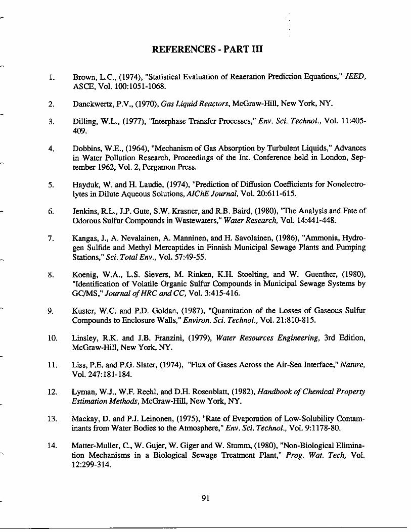
REFERENCES - PART III

1 .

Brown, L.C., (1974), "Statistical Evaluation of Reaeration Prediction Equations," JEED,ASCE, Vol. 100:1051-1068 .

2.

Danckwertz, P.V., (1970), Gas Liquid Reactors, McGraw-Hill, New York, NY.

3 .

Dilling, W.L., (1977), "Interphase Transfer Processes," Env. Sci. Technol., Vol . 11 :405-409 .

4 . Dobbins, W.E., (1964), "Mechanism of Gas Absorption by Turbulent Liquids," Advancesin Water Pollution Research, Proceedings of the Int. Conference held in London, Sep-tember 1962, Vol . 2, Pergamon Press .

5 .

Hayduk, W. and H. Laudie, (1974), "Prediction of Diffusion Coefficients for Nonelectro-lytes in Dilute Aqueous Solutions, AIChE Journal, Vol . 20:611-615.

6 .

Jenkins, R.L., J.P. Gute, S.W. Krasner, and R .B . Baird, (1980), "The Analysis and Fate ofOdorous Sulfur Compounds in Wastewaters," Water Research, Vol. 14:441-448.

7 . Kangas, J., A. Nevalainen, A. Manninen, and H . Savolainen, (1986), "Ammonia, Hydro-gen Sulfide and Methyl Mercaptides in Finnish Municipal Sewage Plants and PumpingStations," Sci. Total Env ., Vol . 57:49-55 .

8 . Koenig, W.A., L.S . Sievers, M. Rinken, K.H. Stoelting, and W. Guenther, (1980),"Identification of Volatile Organic Sulfur Compounds in Municipal Sewage Systems byGC/MS," Journal of HRC and CC, Vol . 3 :415-416.

9 .

Kuster, W.C. and P.D. Goldan, (1987), "Quantitation of the Losses of Gaseous SulfurCompounds to Enclosure Walls," Environ. Sci . Technol ., Vol . 21 :810-815 .

10 .

Linsley, R.K. and J.B . Franzini, (1979), Water Resources Engineering, 3rd Edition,McGraw-Hill, New York, NY .

11 .

Liss, P.E. and P.G. Slater, (1974), "Flux of Gases Across the Air-Sea Interface," Nature,Vol. 247:181-184.

12 .

Lyman, W.J., W.F. Reehl, and D.H. Rosenblatt, (1982), Handbook of Chemical PropertyEstimation Methods, McGraw-Hill, New York, NY .

13 .

Mackay, D. and P.J. Leinonen, (1975), "Rate of Evaporation of Low-Solubility Contam-inants from Water Bodies to the Atmosphere," Env. Sci . Technol ., Vol . 9:1178-80.

14. Matter-Muller, C., W. Gujer, W. Giger and W . Stumm, (1980), "Non-Biological Elimina-tion Mechanisms in a Biological Sewage Treatment Plant," Prog. Wat. Tech, Vol .12:299-314 .

91

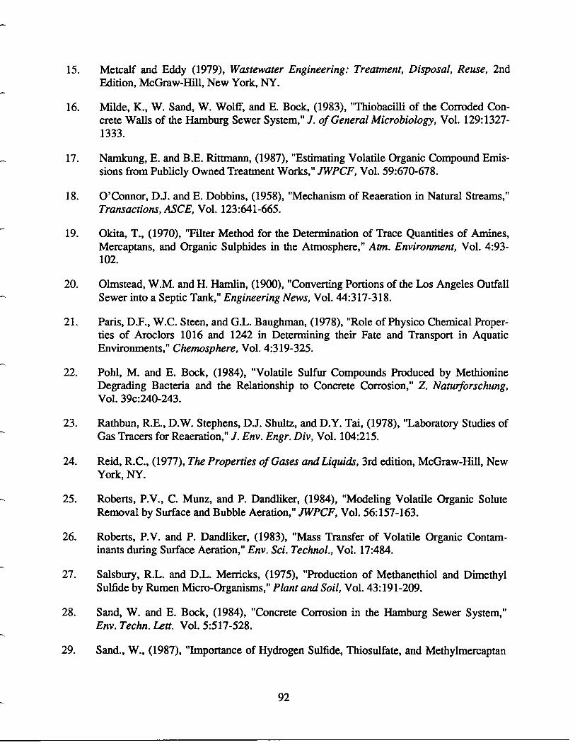
15 .

Metcalf and Eddy (1979), Wastewater Engineering : Treatment, Disposal, Reuse, 2ndEdition, McGraw-Hill, New York, NY.

16 . Milde, K., W. Sand, W. Wolff, and E. Bock, (1983), "Thiobacilli of the Corroded Con-crete Walls of the Hamburg Sewer System," J. of General Microbiology, Vol . 129:1327-1333 .

17 .

Namkung, E. and B.E. Rittmann, (1987), "Estimating Volatile Organic Compound Emis-sions from Publicly Owned Treatment Works," JWPCF, Vol . 59:670-678 .

18 .

O'Connor, D.J. and E. Dobbins, (1958), "Mechanism of Reaeration in Natural Streams,"Transactions, ASCE, Vol. 123:641-665.

19 . Okita, T., (1970), "Filter Method for the Determination of Trace Quantities of Amines,Mercaptans, and Organic Sulphides in the Atmosphere," Atm. Environment, Vol . 4:93-102.

20 .

Olmstead, W.M. and H. Hamlin, (1900), "Converting Portions of the Los Angeles OutfallSewer into a Septic Tank," Engineering News, Vol. 44:317-318 .

21 . Paris, D.F., W.C. Steen, and G.L. Baughman, (1978), "Role of Physico Chemical Proper-ties of Aroclors 1016 and 1242 in Determining their Fate and Transport in AquaticEnvironments," Chemosphere, Vol. 4:319-325.

22 . Pohl, M. and E. Bock, (1984), "Volatile Sulfur Compounds Produced by MethionineDegrading Bacteria and the Relationship to Concrete Corrosion," Z . Naturforschung,Vol. 39c:240-243 .

23 .

Rathbun, R.E., D.W. Stephens, D .J. Shultz, and D .Y. Tai, (1978), "Laboratory Studies ofGas Tracers for Reaeration," J. Env. Engr. Div, Vol. 104:215 .

24.

Reid, R.C., (1977), The Properties of Gases and Liquids, 3rd edition, McGraw-Hill, NewYork, NY .

25 .

Roberts, P.V., C. Munz, and P. Dandliker, (1984), "Modeling Volatile Organic SoluteRemoval by Surface and Bubble Aeration," JWPCF, Vol. 56:157-163.

26 .

Roberts, P.V. and P. Dandliker, (1983), "Mass Transfer of Volatile Organic Contam-inants during Surface Aeration," Env. Sci. Technol ., Vol. 17:484.

27 .

Salsbury, R.L. and D .L. Merricks, (1975), "Production of Methanethiol and DimethylSulfide by Rumen Micro-Organisms," Plant and Soil, Vol. 43 :191-209.

28 .

Sand, W. and E. Bock, (1984), "Concrete Corrosion in the Hamburg Sewer System,"Env. Techn. Lett. Vol. 5:517-528.

29 .

Sand., W., (1987), "Importance of Hydrogen Sulfide, Thiosulfate, and Methylmercaptan

92

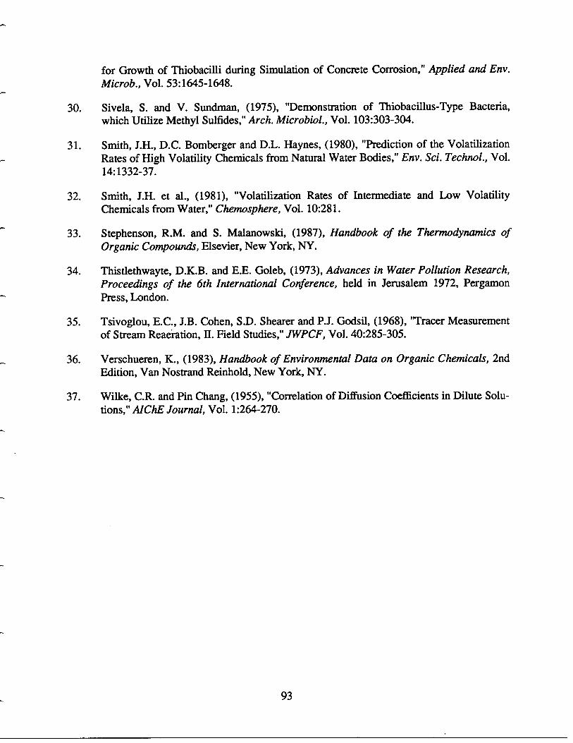
for Growth of Thiobacilli during Simulation of Concrete Corrosion," Applied and Env.Microb., Vol . 53:1645-1648 .

30.

Sivela, S. and V. Sundman, (1975), "Demonstration of Thiobacillus-Type Bacteria,which Utilize Methyl Sulfides," Arch. Microbiol., Vol . 103:303-304 .

31 . Smith, J.H., D.C. Bomberger and D .L. Haynes, (1980), "Prediction of the VolatilizationRates of High Volatility Chemicals from Natural Water Bodies," Env. Sci. Technol., Vol .14:1332-37 .

32 .

Smith, J.H. et al., (1981), "Volatilization Rates of Intermediate and Low VolatilityChemicals from Water," Chemosphere, Vol . 10:281 .

33 .

Stephenson, R.M. and S. Malanowski, (1987), Handbook of the Thermodynamics ofOrganic Compounds, Elsevier, New York, NY .

34 . Thistlethwayte, D.K.B. and E.E. Goleb, (1973), Advances in Water Pollution Research,Proceedings of the 6th International Conference, held in Jerusalem 1972, PergamonPress, London .

35 .

Tsivoglou, E.C., J.B . Cohen, S.D. Shearer and P.J. Godsil, (1968), "Tracer Measurementof Stream Reaeration, II. Field Studies," JWPCF, Vol. 40:285-305 .

36.

Verschueren, K., (1983), Handbook of Environmental Data on Organic Chemicals, 2ndEdition, Van Nostrand Reinhold, New York, NY .

37 .

Wilke, C.R. and Pin Chang, (1955), "Correlation of Diffusion Coefficients in Dilute Solu-tions," AIChE Journal, Vol. 1:264-270 .

93

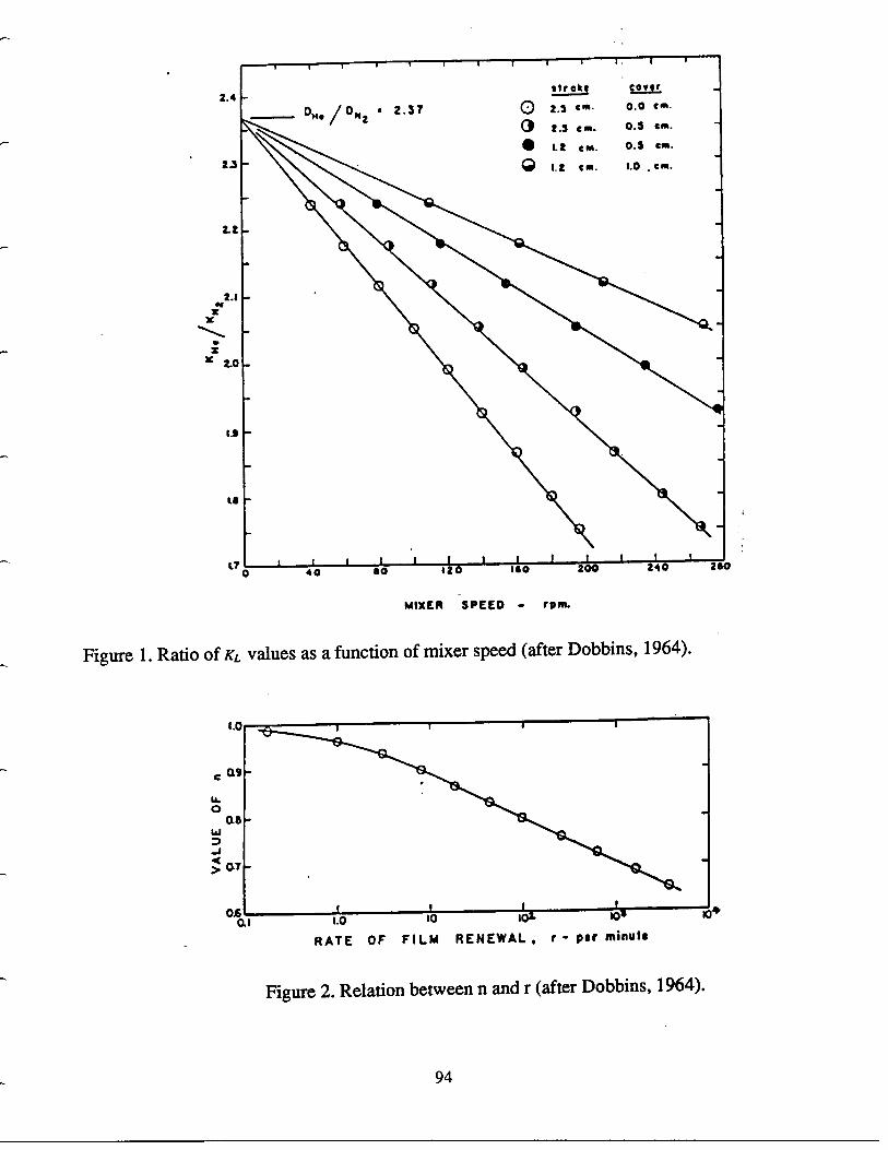
2.4

23

22

N2.1

Y

SY 2.0

1 .1

LA

L10

W0 asWMJ

07 -

0.61

c

Q

I 140

1 1so

1 II120

1160

MIXER SPEED - rpm.

Figure 1 . Ratio of KL values as a function of mixer speed (after Dobbins, 1964) .

1 .0

ea

I II200

94

1240 280

Figure 2. Relation between n and r (after Dobbins, 1964) .

11.0

10

10=

1011 10

RATE OF FILM RENEWAL , r - per minute

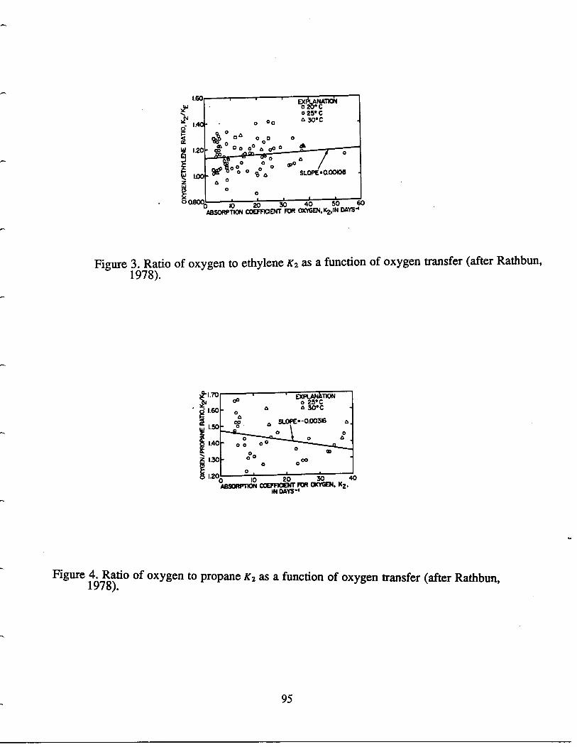
i

o "WOABSORPTION COE20

30

40

50

60FFICIENT FOR OXYGEN, K2,IN DAYS-

Figure 3. Ratio of oxygen to ethylene K2 as a function of oxygen transfer (after Rathbun,1978).

1 .70

1 .60

w 1.50

I.40

1.30

1.200

10

20

30

40ABSORPTION COEFFI00tT FOR OXYGEN . K2 .

IN DAYS''

Figure 4. Ratio of oxygen to propane K2 as a function of oxygen transfer (after Rathbun,1978).

95

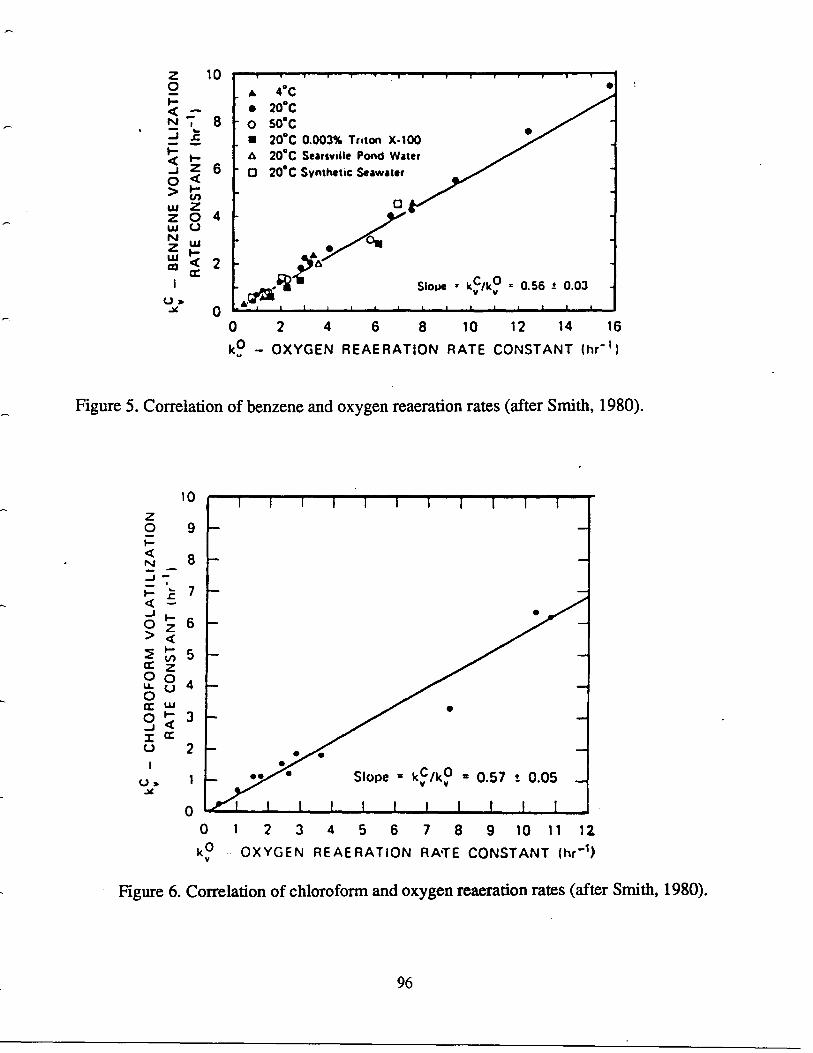
z

100IN ; 8

…

J LI…-J

Z6

…

F-…

N

z o 4W UN WZm Q 2

IU>Y 0

0

2

4

6

8

10

12

14

16

k9 - OXYGEN REAERATION RATE CONSTANT (hr-1 )

Figure 5. Correlation of benzene and oxygen reaeration rates (after Smith, 1980) .

10z…

9

…

_ 8N_J~- L 7…

-J…

Z 6…

cN 5

…

ZLL OU 4OCr. UjH…

Q 3

_ ©CU 2 -

ISlope = kC/k? = 0.57 t 0.05

0 1II1I11I1I

0

1

2

3

4

5

6

7

8

9 10 11 12ko OXYGEN REAERATION RATE CONSTANT (hr -')

Figure 6. Correlation of chloroform and oxygen reaeration rates (after Smith, 1980) .

96

0.5

Figure 7 . Correlation of Diffusivities and mass transfer coefficients (after Smith, 1980) .

0.6 0.7

0.8

0.9

1 .0

kC /kO/kO

97

1 .0

0.9

0.8

0.7

0.600.0U or0

0.5

0.4

0.3

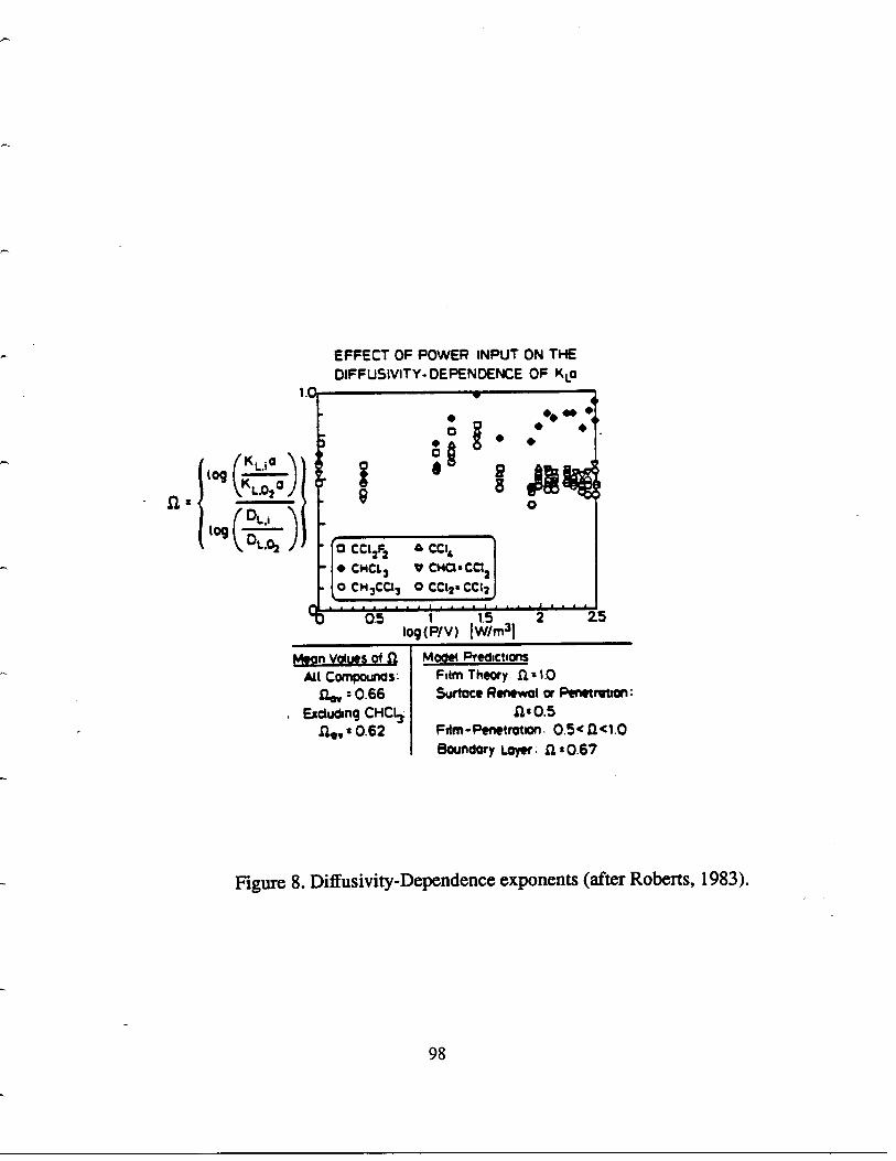
to

n =

logD j. .

D1.,02

EFFECT OF POWER INPUT ON THEDIFFUSIVITY- DEPENDENCE OF K La

1 .0,

a0

…

* MA 4' CC'-6…

CHCL3 v CHCI…CCl2

…

o CH 3CC13 0 CC12& C02

x. . . .0.5 . . . ; . . . .15 . . . .2 . …

25log(P/V) (W/m3]

mean values ofaAll Compounds :no, : 0.66

Excluding CHC13S1,1,=0.62

98

Model PredictionsFilm Theory . ft=1 .0Surtace Renewal or Penetration

9130.5Film-Penetration . 0.5<a<1.0Boundary Layer . A = 0.67

…

8

Figure 8. Diffusivity-Dependence exponents (after Roberts, 1983) .

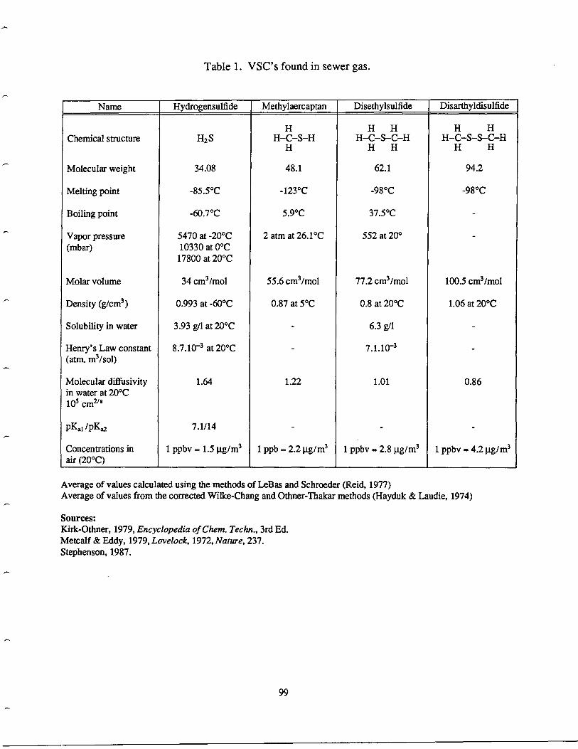
Table 1 . VSC's found in sewer gas .

Average of values calculated using the methods of LeBas and Schroeder (Reid, 1977)Average of values from the corrected Wilke-Chang and Othner-Thakar methods (Hayduk & Laudie, 1974)

Sources :Kirk-Othner, 1979, Encyclopedia of Chem. Techn ., 3rd Ed .Metcalf &Eddy, 1979, Lovelock, 1972, Nature, 237 .Stephenson, 1987 .

99

Name Hydrogensulfide Methylaercaptan Disethylsulfide Disarthyldisulfide

Chemical structure H2SH

H-C-S-HH H

H-C-S-C-HH H

H-C-S-S-C-H

Molecular weight 34.08

H

48.1

H H

62.1

H H

94.2

Melting point -85.5©C -123©C -98©C -98©C

Boiling point -60.7©C 5.9©C 37.5©C -

Vapor pressure 5470 at -20©C 2 atm at 26.1©C 552 at 20© -(mbar) 10330 at 0©C

17800 at 20©C

Molar volume 34 cm3/mol 55.6 cm3/mol 77.2 cm3/mol 100.5 cm3/mol

Density (g/cm3 ) 0.993 at -60©C 0.87 at 5©C 0.8 at 20©C 1.06 at 20©C

Solubility in water 3.93 g/l at 20©C - 6.3 g/l -

Henry's Law constant 8.7.10-3 at 20 ©C - 7.1.10-3 -(atm. m3/sol)

Molecular diffusivity 1.64 1.22 1 .01 0.86in water at 20©Cl05 cm21s

PKa1 /PKa2 7.1/14 - - -

Concentrations in 1 ppbv = 1 .5 °g/m3 1 ppb = 2.2 p.g/m3 1 ppbv = 2 .8 °g/m3 1 ppbv = 4 .2 p.g/m3air (20©C)