CAUSATION, STATISTICS, AND THE LAW - CMU · CAUSATION, STATISTICS, AND THE LAW.DOC 2/8/2008 2:43:00...

CAUSATION, STATISTICS, AND THE LAW.DOC 2/8/2008 2:43:00 PM

101

CAUSATION, STATISTICS, AND THE LAW

Richard Scheines*

INTRODUCTION

More and more, judges and juries are being asked to handle torts and other cases in which establishing liability involves understanding large bodies of complex scientific evidence. When establishing causation is involved, the evidence can be diverse, can involve complicated statistical models, and can seem impenetrable to non-experts. Since the decision in Daubert v. Merril Dow Pharms., Inc.1 in 1993, judges cannot simply admit expert testimony and other technical evidence and let jurors decide the verdict. Judges now must rule on which experts are admissible and which are inadmissible, and they must base their ruling at least partly on the status of the scientific evidence about which the expert will testify. 2 This article is intended to provide judges with an accessible methodological overview of causal science.

Part I of this article will explain the nature of causal claims in the realm of judicial evidence. Part II will address why these claims are difficult to prove scientifically and identify the different kinds of evidence typically used to prove causal claims. Part III will explain how the discipline of statistics fits into the science of establishing causal claims. Finally, part IV will

* Dr. Scheines is a Professor (and Head) of Philosophy at Carnegie Mellon University, with courtesy appointments in the Department of Machine Learning and the Human-Computer Interaction Institute.

1 Daubert v. Merrell Dow Pharms., Inc., 509 U.S. 579 (1993). 2 Id. at 592–93.


102 JOURNAL OF LAW AND POLICY

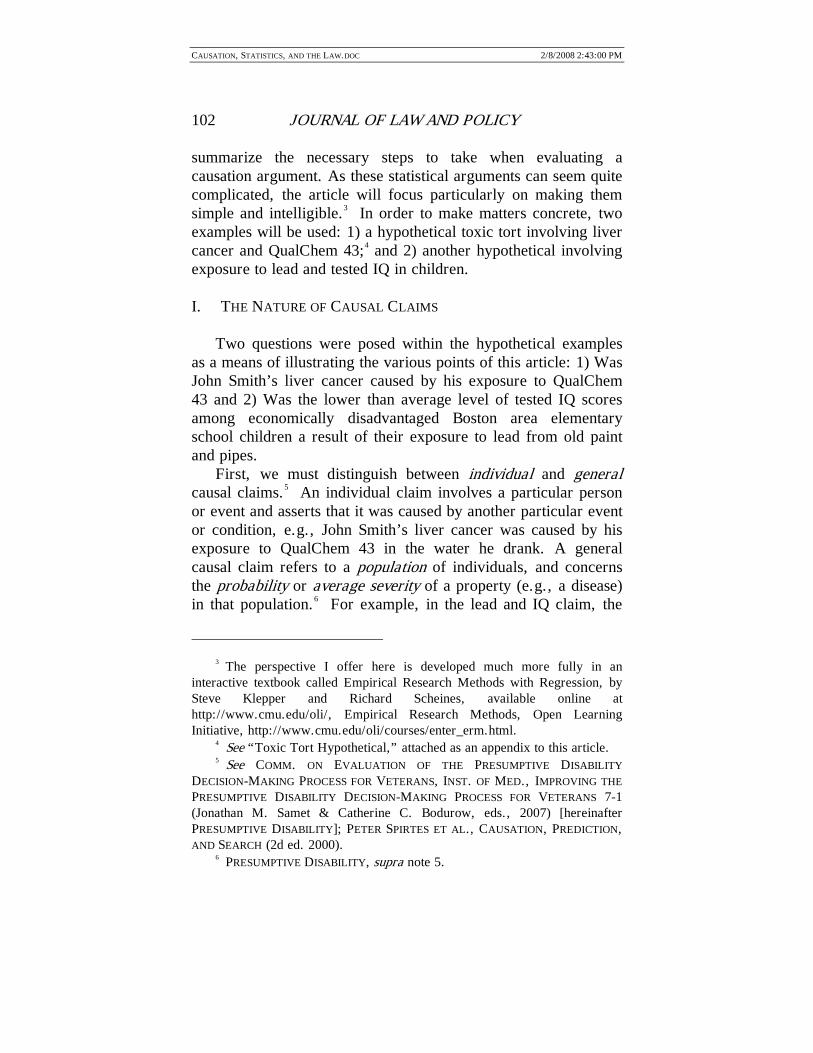
summarize the necessary steps to take when evaluating a causation argument. As these statistical arguments can seem quite complicated, the article will focus particularly on making them simple and intelligible.3 In order to make matters concrete, two examples will be used: 1) a hypothetical toxic tort involving liver cancer and QualChem 43;4 and 2) another hypothetical involving exposure to lead and tested IQ in children.

I. THE NATURE OF CAUSAL CLAIMS

Two questions were posed within the hypothetical examples as a means of illustrating the various points of this article: 1) Was John Smith’s liver cancer caused by his exposure to QualChem 43 and 2) Was the lower than average level of tested IQ scores among economically disadvantaged Boston area elementary school children a result of their exposure to lead from old paint and pipes.

First, we must distinguish between individual and general causal claims.5 An individual claim involves a particular person or event and asserts that it was caused by another particular event or condition, e.g., John Smith’s liver cancer was caused by his exposure to QualChem 43 in the water he drank. A general causal claim refers to a population of individuals, and concerns the probability or average severity of a property (e.g., a disease) in that population.6 For example, in the lead and IQ claim, the

3 The perspective I offer here is developed much more fully in an

interactive textbook called Empirical Research Methods with Regression, by Steve Klepper and Richard Scheines, available online at http://www.cmu.edu/oli/, Empirical Research Methods, Open Learning Initiative, http://www.cmu.edu/oli/courses/enter_erm.html.

4 See “Toxic Tort Hypothetical,” attached as an appendix to this article. 5 See COMM. ON EVALUATION OF THE PRESUMPTIVE DISABILITY

DECISION-MAKING PROCESS FOR VETERANS, INST. OF MED., IMPROVING THE PRESUMPTIVE DISABILITY DECISION-MAKING PROCESS FOR VETERANS 7-1 (Jonathan M. Samet & Catherine C. Bodurow, eds., 2007) [hereinafter PRESUMPTIVE DISABILITY]; PETER SPIRTES ET AL., CAUSATION, PREDICTION, AND SEARCH (2d ed. 2000).

6 PRESUMPTIVE DISABILITY, supra note 5.


CAUSATION, STATISTICS, AND THE LAW 103

population is economically disadvantaged Boston area elementary school children, the property is tested IQ, and the claim is that the average level of the property is different than it would have been had the population not been exposed to lead. The general claim does not entail that every child in the population who was exposed to lead lost IQ points, nor does it claim that every child with a lower than average tested IQ was so because of exposure to lead. It is a claim about the average IQ in the population, and how that might have differed if the children had not been exposed to lead from old paint and old pipes.

In both cases the essential claim is counterfactual: the effect would have been different if the cause had been different. 7 For John Smith, the claim is: had John Smith not been exposed to QualChem 43, he would not have gotten liver cancer. For lead and IQ, the claim is: had the population of Boston children not been exposed to lead from old paint and pipes, their average IQ would have been higher.

In both cases the counterfactual supposition is a bit vague. How are we to imagine John Smith’s life without QualChem 43? Do we imagine he avoided exposure to QualChem 43 by having lived in a different location? By having been wealthy and only consuming bottled water? How are we to imagine the Boston children’s life without lead? Are they allowed to relocate to Phoenix, Arizona, where much of the infrastructure is so new that lead doesn’t occur in paint and pipes? No. What we mean to suppose, in both cases, is that everything was as close to the way it actually happened as possible, except for removing the “cause.” For John Smith we imagine that he lived exactly the same life, but that his drinking water contained no QualChem 43. For the Boston children, we imagine that they lived exactly the same life, that their paint was identical in appearance but contained no lead, and that their pipes contained no lead but were

7 For more information about a counterfactual, and how it relates to

causation, see generally CAUSATION AND COUNTERFACTUALS (John D. Collins, Ned Hall & L. A. Paul, eds., 2004).



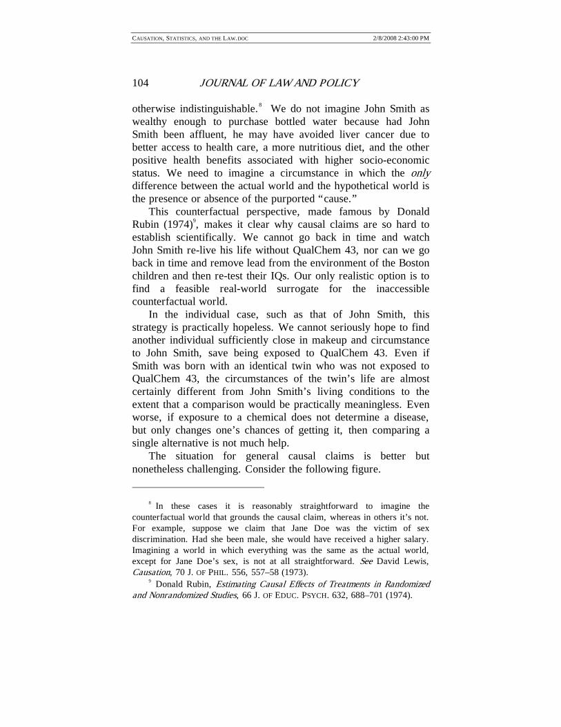
otherwise indistinguishable. 8 We do not imagine John Smith as wealthy enough to purchase bottled water because had John Smith been affluent, he may have avoided liver cancer due to better access to health care, a more nutritious diet, and the other positive health benefits associated with higher socio-economic status. We need to imagine a circumstance in which the only difference between the actual world and the hypothetical world is the presence or absence of the purported “cause.”

This counterfactual perspective, made famous by Donald Rubin (1974)9, makes it clear why causal claims are so hard to establish scientifically. We cannot go back in time and watch John Smith re-live his life without QualChem 43, nor can we go back in time and remove lead from the environment of the Boston children and then re-test their IQs. Our only realistic option is to find a feasible real-world surrogate for the inaccessible counterfactual world.

In the individual case, such as that of John Smith, this strategy is practically hopeless. We cannot seriously hope to find another individual sufficiently close in makeup and circumstance to John Smith, save being exposed to QualChem 43. Even if Smith was born with an identical twin who was not exposed to QualChem 43, the circumstances of the twin’s life are almost certainly different from John Smith’s living conditions to the extent that a comparison would be practically meaningless. Even worse, if exposure to a chemical does not determine a disease, but only changes one’s chances of getting it, then comparing a single alternative is not much help.

The situation for general causal claims is better but nonetheless challenging. Consider the following figure.

8 In these cases it is reasonably straightforward to imagine the counterfactual world that grounds the causal claim, whereas in others it’s not. For example, suppose we claim that Jane Doe was the victim of sex discrimination. Had she been male, she would have received a higher salary. Imagining a world in which everything was the same as the actual world, except for Jane Doe’s sex, is not at all straightforward. See David Lewis, Causation, 70 J. OF PHIL. 556, 557–58 (1973).

9 Donald Rubin, Estimating Causal Effects of Treatments in Randomized and Nonrandomized Studies, 66 J. OF EDUC. PSYCH. 632, 688–701 (1974).



Figure 1: Counter factual vs. Actual Populations Suppose that the box in the upper left of

Figure 1 (Actual Population 1) represents the actual population of Boston school children we are considering. The box below it (Counterfactual Population 1) represents a counterfactual world we cannot access: a world involving the same children living the same life, save that we have gone back in time and intervened to remove the lead from the paint and the pipes but otherwise left things alone. The box in the upper right (Actual Population 2) represents what we can obtainanother group of actual children that are not exposed to lead. For example, we might consider children from Phoenix, Arizona that are otherwise as similar as possible to the Boston children in our original population. The problem, of course, is that such a group will inevitably differ in lots of ways, many of which might well be relevant to their tested IQ.

Counterfactual Population 1:

Changed to eliminate lead

Average(IQ) = ??

Actual Population 1:

Average(IQ) = X

Causation

Actual Population 2: No lead exposure

observed

Average(IQ) = ??



II. THE KINDS OF EVIDENCE FOR CAUSAL CLAIMS

There are three kinds of evidence typically used in scientifically establishing general level causal claims: clinical trials, observational studies, and biological/toxicological studies. 10

A. Clinical Trials

Sir Ronald Fisher, the brilliant and prolific British statistician, provided in the 1930s what is still the gold standard today for causal inference: the randomized trial (“RT”). 11 In its simplest form, an RT randomly splits a population into two subgroups, thus creating two “versions” of the same population,12 and then exposes one sub-population to the cause (the “treated” group) and does not expose one to the cause (the “control” group). The frequency of the effect in the two groups provides evidence of the probability of the effect in the two populations we seek: one in which the cause is present, and an identical copy in which the cause is not present. Subtleties abound, but the basic strategy is sound and taught in every introductory research methods course.

The problem, of course, is that performing an RT is either ethically or practically impossible in a number of situations. We simply cannot intentionally expose half a population of children to lead or QualChem 43. There are essentially two recourses to an RT: 1) we can conduct an observational study and statistically

10 For a much more detailed discussion, see PRESUMPTIVE DISABILITY, supra note 5 at 117–38; CTRS FOR DISEASE CONTROL AND PREVENTION, DEP’T OF HEALTH AND HUMAN SVCS, 2004 SURGEON GENERAL’S REPORT—THE HEALTH CONSEQUENCES OF SMOKING (2004); FEDERAL JUDICIAL CENTER, REFERENCE MANUAL ON SCIENTIFIC EVIDENCE (2d ed. 2000).

11 RONALD A. FISHER, STATISTICAL METHODS FOR RESEARCH WORKERS (4th ed., Edinburgh: Oliver and Boyd 1932) (1925).

12 They are not literally the same, of course. Because they were formed by randomly assigning individuals to one subgroup or the other, we can expect both groups to share the same statistically measurable qualities (e.g. , same percentage of smokers and non-smokers, same percentage of lower, middle, and upper class people, etc.). Thus, when viewed as whole groups, they are statistically identical.



adjust for naturally occurring differences in two populations, or 2) we can perform very small versions of RTs on animals we deem appropriate for testing despite the inflicted harm, e.g., rodents.

B. Observational Studies

Observational studies involve human populations in which we do not control exposure to a cause.13 Thus, we are typically comparing an actual subpopulation whose members were exposed to a cause and another subpopulation whose members were not exposed, e.g., Actual Population 1 as compared to Actual Population 2 in

Figure 1. For example, in examining whether poverty causes crime, sociologists might collect data on a subpopulation of people below the poverty line and compare them to a subpopulation of people above the poverty line. The study is “observational” if the sociologist does not intervene to affect whether any of the subjects were above or below poverty.

In some cases, the “cause” is not a simple on-off event like “below the poverty line” versus “above the poverty line,” but rather, the cause is a factor that can take on values across a large range, e.g., yearly income in dollars. For example, another sociologist might sample a population and measure each individual’s level of income according to dollars earned per year and their criminal activity according to the number of days spent in jail.

13 PAUL R. ROSENBAUM, OBSERVATIONAL STUDIES 2 (2d ed. 2002).



An observational study that involves health or disease is called an “epidemiological study.”14 A classic example is a “cohort” study in which groups which vary by exposure are tracked over time and compared as to some health outcome like cancer. For example, Takeshi Hirayama (1984)15 tracked lung cancer mortality for over 16 years in over 90,000 non-smoking wives in Japan, some of whom were married to non-smokers, some to moderate smokers, some to heavy smokers.

Another type of epidemiological study is a “case-control” study: instead of comparing the frequency of an effect in two subpopulations that vary as to the cause, epidemiologists compare the level of exposure to the cause in two subpopulations that differ on the effect. For example, in the toxic tort hypothetical involving QualChem 43, epidemiologists employed by the Mississippi Department of Public Health compared the rate of exposure to QualChem 43 between a group of liver cancer patients and a group of similar patients without liver cancer.

The essential methodological issue in observational studies is that populations that vary in level of exposure to the cause might vary in other ways that are relevant to the effect. This is generally called the problem of “confounding” and how scientists address this problem will be discussed later in the section on statistics.

C. Biological/Toxicological Studies

In many cases, animals like rats, mice, rabbits, or chimps seem to have physiological pathways or components sufficiently similar to our own that we believe we can extrapolate from what happens in experiments with animals to what would happen in similar experiments with humans. Biologists frequently perform controlled experiments on rodents to garner evidence for whether

14 KENNETH J. ROTHMAN & SANDER GREENLAND, MODERN

EPIDEMIOLOGY (3d ed. 1998). 15 Takeshi Hirayama, Cancer Mortality in Nonsmoking Women With

Smoking Husbands Based on a Large-Scale Sohort Study in Japan, 13 PREVENTIVE MEDICINE 680, 680–90 (1984).



some chemical causes cancer. They expose some rodents to a “control” and others that are genetically identical and raised in the same environment to the chemical of interest, and then biologists compare the frequency of cancerous tumors. For example, in the hypothetical toxic tort involving QualChem 43, rats were used in a study to examine the toxicology of QualChem 43 with respect to liver cancer.

The degree to which such studies are relevant to the causal claim in humans depends upon 1) whether the physiological mechanism by which the chemical produces the disease in the experimental animals is similar to the mechanism that would produce the disease in humans, and 2) whether we can translate animal doses to human doses in terms of equivalent toxicity. For example, in the toxicological study on rats in the toxic tort hypothetical, “researchers believe that both liver and kidney cancer are initiated by perturbations in cell differentiation,” and therefore they believe that the mechanisms are similar enough in humans to make the animal results relevant. In terms of the dosage, the researchers responsible for the study believe that they can roughly translate the dosage given to each group of rats into human units, and in this case, the number of lifetime equivalent doses to which John Smith was exposed. Thus the first group of rats was exposed to the equivalent of twice the dose of QualChem 43 that John Smith received in his lifetime.

III. STATISTICS AND CAUSATION

Studies reported in peer reviewed scientific journals can seem filled with statistical tables and jargon. This section will identify what is essential about what the statistics indicate while also explaining what is not essential and why.

The scientific case for causation is usually made in two stages. First, we make the prima facie case that there is a statistical association between the purported cause and the effect. As several different causal arrangements can produce statistical association, however, association by itself does not prove causation. In the second stage of making a scientific case for causation, we attempt to eliminate all other possible explanations



of this association. In both stages, statistical methods are involved.



A. Making a Prima Facie Case for Causation: Establishing an Association


Prob(Effect | Exposed to Cause)

Counterfactual Population 1:

Prob(Effect | Cause removed)

Causal Association


Prob(Effect | Not Exposed to Cause)

Observed Association

Figure 2: Causation vs. Association16

Consider Figure 2, which is a slightly revised version of

Figure 1. To establish causation, we need to show that the effect is more probable among those exposed to the cause than it would have been among the same group, had they not been exposed to the cause. In Figure 2, this translates into comparing the two columns in Table 1:

16 The expression Prob(Effect | Exposed to Cause) denotes the probability

of the effect among those Exposed to the Cause. It also might be referred to as the conditional probability of the Effect, given Exposure to the Cause. In the Counterfactual Population 1, the notation Prob(Effect | Cause removed) shows “removed” in italics to emphasize that we are intervening to remove the cause.



Actual Population 1 Counterfactual Population 1

Prob(Effect | Exposed to Cause) Prob(Effect | Cause removed)

Table 1: Causal Association

The difference in these probabilities is the causal effect, and it is the Holy Grail of Causal Science.17 There are two major scientific challenges to getting there:

1. Counterfactual populations are unobservable: because we cannot go back in time and remove the cause from the actual exposed population, we are forced to compare two distinct actual populations. 2. Probabilities are unobservable: we can only study a finite sample of individuals and then make a statistical inference about the probabilities from the observed frequencies in the sample. Let us focus first on the second problem, in which the use of

statistics is, if not simple, fairly straightforward. If we can do a randomized trial, then we can compare two groups that we expect to be identical, and thus overcome the first obstacle. That is, in an RT we assume the difference in Table 2 will correspond to the difference in Table 1.

Actual Population 1 Actual Population 2

Prob(Effect | Assigned to: Exposed to the Cause)

Prob(Effect | Assigned to: Not Exposed to the Cause)

Table 2: Association in a Randomized Trial

Although the challenge of unobservable probabilities must still be overcome in a RT, the discipline of statistics provides us with a rigorous theory of how to do so. For example, consider a fictitious (and unethical) study involving QualChem 43 and liver cancer involving a sample of 100 people, half of whom were

17 SPIRTES ET AL., supra note 5; Rubin, supra note 9, at 688–701.



chosen at random and intentionally exposed to Qualchem 43 and the other half intentionally not exposed. In this example, and several that follow, the true causal process was simulated on a computer, and samples were pseudo-randomly drawn from the population that the computer model defined. Thus, in each case, when reference is made to the “true” model, such reference is to the computer simulation rather than the real world.

Figure 3 shows hypothetical frequencies of liver cancer 20 years later in both the exposed and unexposed groups. The left side of the figure shows a bar chart for the group exposed to QualChem 43, about 20% of whom contracted liver cancer, and the right side shows a bar chart for the unexposed group, about 3% of whom developed liver cancer. The difference in the charts reflects the statistical association between liver cancer and QualChem 43, and the association appears to be substantial.

Figure 3: QualChem 43 Trial

Calling the “difference” in the charts an “association” is a little vague without defining what constitutes an association. To discuss the notion of association scientifically, we must have a clear and precise measure of association. We can then estimate the association from data and assess the range of our uncertainty around this estimate. The following section presents three measures of association that are commonly employed: Relative Risk, Odds Ratio, and Correlation.



1. Relative Risk

The most common measure of association in disease and exposure studies is called the relative risk, or RR. The relative risk is defined as:

exposednot #disease with exposednot #exposed#disease with exposed#

)unexposed()exposed(

==incidence

incidenceRR

In Figure 3, the relative risk for liver cancer of QualChem 43 is .202 / .032 = 6.31. A relative risk of 1.0 reflects that the frequency of disease among the exposed is the same as among the unexposed, thereby indicating that there is zero association. A relative risk of 10 means that the rate of disease among the exposed is ten times as high as among the unexposed.

A high relative risk does not imply a high absolute risk in the population. If, for example, one in a million unexposed individuals gets the disease but 10 in a million exposed individuals get the disease, then the relative risk is 10, even though the chances of getting the disease among those exposed is still only 1 in 100,000.

Another measure of association that is commonly used in case-control studies like the one described in the toxic tort hypothetical discussed later is the odds ratio, or OR:

exposednot &diseasewithout # exposednot &diseasewith #exposed&disease without #exposed&diseasewith #

=OR

No matter which measure of association one uses, however, the key statistical question is whether from the observed association we can infer that there is a real (population) association.

2. Hypothesis Tests and P-values

The most common statistical method with which to make this inference is called a hypothesis test, particularly the “null” hypothesis that the real association is zero and the observed



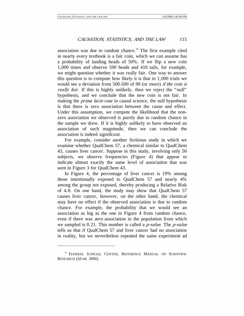
association was due to random chance.18 The first example cited in nearly every textbook is a fair coin, which we can assume has a probability of landing heads of 50%. If we flip a new coin 1,000 times and observe 590 heads and 410 tails, for example, we might question whether it was really fair. One way to answer this question is to compute how likely it is that in 1,000 trials we would see a deviation from 500-500 of 90 (or more) if the coin is really fair. If this is highly unlikely, then we reject the “null” hypothesis, and we conclude that the new coin is not fair. In making the prima facie case in causal science, the null hypothesis is that there is zero association between the cause and effect. Under this assumption, we compute the likelihood that the non-zero association we observed is purely due to random chance in the sample we drew. If it is highly unlikely to have observed an association of such magnitude, then we can conclude the association is indeed significant.

For example, consider another fictitious study in which we examine whether QualChem 57, a chemical similar to QualChem 43, causes liver cancer. Suppose in this study, involving only 50 subjects, we observe frequencies (Figure 4) that appear to indicate almost exactly the same level of association that was seen in Figure 3 for QualChem 43.

In Figure 4, the percentage of liver cancer is 19% among those intentionally exposed to QualChem 57 and nearly 4% among the group not exposed, thereby producing a Relative Risk of 4.8. On one hand, the study may show that QualChem 57 causes liver cancer, however, on the other hand, the chemical may have no effect if the observed association is due to random chance. For example, the probability that we would see an association as big as the one in Figure 4 from random chance, even if there was zero association in the population from which we sampled is 0.21. This number is called a p-value. The p-value tells us that if QualChem 57 and liver cancer had no association in reality, but we nevertheless repeated the same experiment ad

18 FEDERAL JUDICIAL CENTER, REFERENCE MANUAL ON SCIENTIFIC

RESEARCH (2d ed. 2000).



infinitum, then we would still expect to observe as large an association as the one in Figure 4 over 20% of the time. Since the observed association in Figure 4 could so easily be explained by random chance, it is said to be statistically insignificant. In the computer simulation for QualChem 57 and liver cancer, QualChem 57 had no effect on liver cancer, there was no association whatsoever in the underlying model (RR = 1.0), and the observed RR = 4.8 was entirely due to random sampling variation.

Figure 4: QualChem 57 Trial

Associations reported in studies are not typically considered statistically significant unless the chances of seeing that large an association just from random chance are less than .05, or one in twenty. This is a completely arbitrary convention, and can be quite misleading when interpreted as a strict threshold, or decision rule. In Figure 3, for example, the association (RR= 6.31) in the sample has a p-value = .058 which would be considered statistically insignificant at a threshold of .05 even though the Relative Risk in the underlying model simulated in the computer was 4.4 (probabilities equal to 22% for exposed and 5% for unexposed).

3. Confidence Intervals

Confidence intervals are closely related to p-values and serve as an attempt to capture the uncertainty in a parameter estimate that is due to random chance, or “sampling variability.” For



example, in a political poll that reports the percentage of people who approve of George Bush’s performance as President, the result might be described as “accurate to within plus or minus three percentage points.”19 Statistically speaking, this means if the survey was repeated numerous times, each with the same number of subjects, and each time we reported our findings as an interval that was within three percentage points of the percentage that we observed, then 95% of the time our interval would contain the true percentage. The 95% is the “confidence level,” and again, using 95% is a purely arbitrary convention.

With a bigger sample, the 95% confidence interval gets narrower, and the results of the study become more precise. Many political polls, for example, sample the opinions of just over 1,000 voters.20 With this sample size, a 95% confidence interval usually amounts to plus or minus three percentage points. If the pollsters interviewed 10,000 voters, then a 95% confidence interval would be approximately plus or minus 1 percentage point. 21

Adjusting the confidence level also changes the size of the interval. If the political pollsters took a sample of 1,000, but reported a 50% confidence interval instead of a 95% confidence interval, the results would be accurate within slightly more than one percentage point.

In the case of establishing an association to make a prima facie case for causation, the parameter of interest is the size of the association in the population. In Figure 3, for example, the sample drawn from the population exhibits a relative risk of 6.31. Maybe the real RR (the RR in the population, which we cannot observe) is actually 6.29. Maybe the RR in the population is 1.0 (no association). The 95% confidence interval around our estimated RR= 6.31 includes a RR of 1.0, and therefore, a

19 See, e.g. , PollingReport.Com, President Bush: Job Ratings, http:// www.pollingreport.com/BushJob1.htm (last visited Nov. 26, 2007).

20 See, e.g. , id. 21 To see how the confidence level, confidence interval, and sample size

interact, see the Sample Size Calculator at www.surveysystem.com/sscalc.htm (last visited Nov. 26, 2007).



population with no association is within our 95% confidence interval. A 90% interval would not include a RR of 1.0. Similarly, in the case-control study in the toxic tort hypothetical, Exhibit C shows 90% and 95% confidence intervals for the estimated odds-ratio of 3.2. As you can see, the 90% interval is nested within the 95%, and the 95% interval includes a RR of 1.0 while the 90% interval does not include the same RR. A 100% interval would have to include all possible levels of association.

The relationship between p-values and confidence intervals is simple. Whatever the observed level of association A, if an X% confidence interval around A meets exactly the number that corresponds to zero association, then the observed level of association A is significant at a p-value of X%.

Figure 5: Confidence level = p-value

For example, in the case-control study in the toxic tort hypothetical, a 94% confidence interval would meet exactly zero, therefore the association is significant at a p-value of .06.

4. Correlation

These points apply equally well in cases in which we are examining a dose-response relationship between quantities that vary across a numerical range, such as exposure to lead and IQ. In that case, the measure of association typically used is the correlation coefficient. The p-value and confidence interval have the same logic for correlation as they do for relative risk, odds ratio, or any other statistical measure of association. For example, in a fictitious experiment (again, simulated in a computer) in which a sample of 160 children were exposed to a

Zero A Association (Observed Assocation)

X% Confidence Interval



random amount of lead for the first seven years of life and then given an IQ test on their seventh birthday, we might observe the scatter-plot of dose-response shown in Figure 6. The blue line represents the best-fitting line (regression line) in which IQ is predicted from lead exposure. The correlation coefficient of -.211 is a measure of association in this type of sample. The p-value of .007 indicates that the probability of observing this large a negative correlation from just random chance is .007. Since .007 is very low, and well below .05 or the other common cutoff .01, the correlation would be considered significant.

Figure 6: Lead and IQ Scatterplot

In these three fictitious cases, we came close to making a prima facie case for the hypothesis that QualChem 43 causes liver cancer (p-value = .058, Figure 3), we failed to make a prima facie case for the hypothesis that QualChem 57 causes



liver cancer (p-value = .21, Figure 4), and we easily made a prima facie case for the hypothesis that lead causes IQ deficits in 7 year olds (p-value = .007, Figure 6).

To summarize, getting to the Holy Grail of Causal Science requires overcoming two obstacles: comparing the right actual populations and making statistical inferences. No matter which populations we compare, to make a prima facie case for causation requires the statistical inference that there is association between the putative cause and the effect. P-values and confidence intervals help us get over the “is there really an association” obstacle.

B. Challenges to the Prima Facie Case

Supposing that we have passed the prima facie test for causation, what more remains in order to establish (and estimate the strength of) a causal relationship? In the case of a randomized trial, nothing. That is because a randomized trial overcomes the first obstacle to establishing causationcomparing the right populations.

In an observational study, however, we cannot assume that a group that was exposed to the cause and another group that was not exposed are otherwise the same. For example, suppose we compare two groups in an observational study: one group that was exposed to QualChem 43 and one group that was unexposed to the chemical. Suppose the first group of 200 lived on the Blue River in Mississippi, where they were exposed to QualChem 43 from the release of the chemical into the Blue River near their houses. Suppose the second group of 200 lived on the Red River in Kansas. Suppose that the relative risk of liver cancer between the two groups was 2.3, which was significant at a p-value = .003 and thus passed the prima facie test with flying colors. Statistically, it is true to say that the chance of observing an RR of 2.3, if there is none in the population, is less than 3 in 1,000. Therefore, let us agree that there is an association between QualChem 43 exposure and liver cancer.

Suppose, however, that the socioeconomic status (“SES”) of the Red River families was on average much higher than the Blue



River families. As a result of their lower SES, the Blue River families are less able to afford to live away from industry and thus more prone to QualChem 43 exposure. Further, as a result of lower SES, Blue River families also tend to consume a more unhealthy diet and more alcohol, both of which cause liver cancer (

Figure 7). The different average SES in the two groups is

called a “confounder,” as it is an alternative, non-causal explanation of the association between QualChem 43 exposure and liver cancer.



Figure 7: Confounding

The big problem is that the size of the observed association has no logical relation to whether it came from confounding or causation.

For example, Figure 8 shows the results of a simulation in which QualChem 43 causes liver cancer, but the casual relationship between the chemical and cancer is weak (RR = 1.33). In the sample of 200 drawn, the observed RR = 1.29 (p-value = 0.11), is not significant at the usual level of .05 or even at the weaker significance level of .10.

Low SES

High Alcohol Consumption

Liver Cancer

Poor Diet

Exposure to QualChem 43

Can’t Afford Housing far from

Industry



Figure 8: Causation, RR= 1.29, p = .11

Figure 9 shows the results of a simulation in which QualChem 43 does NOT cause liver cancer, but is associated with the disease (RR= 2.4) as a result of the confounder SES. In the random sample of 200 drawn in this simulation, the RR is 2.3 with a p-value well under .01results which would pass muster as statistically significant in any court of science or law.



Figure 9: Confounding, RR = 2.3, p < .01

Unfortunately, we do not get to see the “correct graph” in the real world; only the observed RR or some other measure of association. From the above hypotheticals, it should be obvious that association doesn’t prove causation. If the association appears statistically real, that does not mean the association was produced by a causal relationship, but rather, only that it was not produced by random chance.

It is tempting to think that the statistical level of certainty/uncertainty about an association should translate in some way to a level of certainty/uncertainty about whether there is a causal relationship. For example, if in study 1 the RR for chemical A is significant at a p-value of .04, and in study 2 the RR for chemical B is significant at a p-value of .00001, then it is tempting to think that the case for causation is correspondingly stronger for chemical B than it is for chemical A. However, confounding renders this belief inaccurate.

If confounding is plausible, which is almost always the case in an observational study, then the level of statistical uncertainty



about the size of the association has almost nothing to do with the level of uncertainty about the size of the causal effect. 22 The lack of a relationship between the statistical uncertainties of the association and the size of the causal effect cannot be emphasized strongly enough as it is easy to confuse statistical certainty about association (low p-values, tight confidence intervals) with scientific certainty about causation.

As if the worry about confounding wasn’t enough of a challenge to the prima facie case for causation, there are other reasons why an observed association might be spurious, that is, explicable by some non-causal reason. In case control studies like the one described in the hypothetical toxic tort, for example, instead of comparing the frequency of the effect (e.g., liver cancer) among two groups that differ on the cause, epidemiologists compare the frequency of exposure to the cause among two groups that differ on the effect (e.g., a group of liver cancer patients versus a group of otherwise similar patients who do not have liver cancer).23 If the frequency of exposure is different, then an association exists between the cause and the effect.

A common source of spurious association in case-control studies is “recall bias.”24 For example, consider

Figure 10, which shows a causal structure in which actual

exposure to QualChem 43 has no effect on liver cancer, but in which recalled exposure and liver cancer will be associated. This is quite plausible, as liver cancer patients who are asked to recall whether they were exposed to QualChem 43 might be suspicious that some industrial chemical

22 See James M. Robins, Confidence Intervals for Causal Parameters, 7

STATISTICS IN MEDICINE 773, 773-85 (1988); see also James M. Robins, Richard Scheines, Peter Spirtes, & Larry Wasserman, Uniform Consistency in Causal Inference, 90 BIOMETRIKA 491, 491–515 (2003).

23 ROTHMAN & GREENLAND, supra note 14. 24 ROTHMAN & GREENLAND, supra note 14.



emitted by some uncaring chemical company caused their cancer, while similar individuals who are otherwise healthy will have no extra motivation to recall being exposed.

Figure 10: Recall Bias

C. Overcoming Challenges to the Prima Facie Case

1. Statistically Adjusting for Confounding

If an epidemiologist were to compare the Red River group to the Blue River group, they would be well aware that these groups might differ in ways germane to the causal claim at issue. In particular, epidemiologists would almost certainly entertain the idea that the groups differed as to SES. As a result, they would undoubtedly employ the most common strategy in dealing with differences in two populations in an observational study: epidemiologists would measure SES and adjust for the difference statistically. 25 They would compute the association between QualChem 43 and liver cancer that arises because of differences in SES, and then report only the residual association between QualChem 43 and liver cancer that could not be explained by SES.26 The researchers would then test whether this adjusted association could be explained by random chance (natural sample variation). 27

For example, Figure 9 shows a study in which the RR for QualChem 43 and liver cancer is 2.3, which is a significant

25 ROTHMAN & GREENLAND, supra note 14. 26 ROTHMAN & GREENLAND, supra note 14. 27 ROTHMAN & GREENLAND, supra note 14.

Actual Exposure to QualChem43

Liver Cancer

Recalled Exposure



association (p-value < .01). If, however, we adjust the association by controlling for SES, then the RR = 1.17 and is insignificant (p-value = .83). Thus, in this case, QualChem 43 passed the prima facie test but did not withstand challenges to the test.

When the measure of association used is correlation, then by far the most commonly used statistical technique for adjusting for confounders is multiple regression.28 Easy to interpret and use, multiple regression computes the correlation between a putative cause and effect adjusting for any number of “covariates” (measured confounders).

When is the strategy of adjusting for confounders reliable for overcoming challenges to the prima facie test? First, it is only reliable if we have adjusted for all the differences in the two populations that are potential causes of the effect, i.e. if we have controlled for all the potential confounders. Just as our prima facie case for QualChem 43 in the Figure 9 study came undone when we adjusted for SES, another study that showed a significant association after adjusting for SES might come undone when we adjust not only for SES but also for age. Just as the p-value or confidence interval for an unadjusted association between a potential cause X and an effect Y tells us very little about the level of our uncertainty as to whether X is a true cause of Y, the p-value of an adjusted association tells us very little about the level of our uncertainty as to whether X is a true cause of Y. Adjusting for confounders is crucial, but unless we are confident we have measured and adjusted for all the confounders, we cannot quite yet reach for the Holy Grail of Causal Science.

The second major scientific problem in adjusting for confounders is that they must be measured accurately. In many cases, what we can measure is a very noisy approximation of the real thing. For example, consider the case of lead and IQ. If we made a prima facie case that exposure to lead was negatively correlated with IQ, an immediate challenge to inferring causation

28 See FEDERAL JUDICIAL CENTER, REFERENCE MANUAL ON SCIENTIFIC EVIDENCE 179–200 (2d ed. 2000). .



is the spurious association that might arise from parental resources (

Figure 11). Parents with higher levels of resources, financial

and otherwise, will avoid housing that might have lead contamination from paint or pipes (or they will have it repaired), and they will also typically provide more stimulation to their children, especially the type that will result in higher tested IQ, entry into a good school, good college, etc.

Figure 11: Confounder of Lead and IQ: Parental Resources

Thus any study on the causal connection between lead and IQ

should report a correlation adjusted for the level of parental resources. How are we to measure the level of parental resources? Going into the home and extensively surveying and observing the parents would be ideal but also impractical. Sociologists are more likely to ask the mother how many years of education she has completed.29 The number of years of education the mother has completed is a good proxy of for parental resources, but an imperfect one. Unfortunately, statistically adjusting for an imperfect measure of a confounder is the same as partially omitting the confounder altogether. The more imperfect the measure, the more it is akin to omission.

29 See, e.g., J.L. Needleman, S. Geiger & R. Frank, Lead and IQ scores:

a reanalysis, 227 SCIENCE 701, 701-704 (1985).

??

Parental Resources

Lead Exposure Tested IQ



Figure 12: Confounder Measured Poorly

For example, consider a simulated example ( Figure 12) in which lead exposure has no effect on tested IQ.

Thus any observed correlation is spurious and due entirely to parental resources or to random variation in sampling. Further, consider a measure of imperfect parental resources (“PR Measure”): ½ of the variation in the measure is from variation in parental resources, but ½ is from unrelated noise. Table 3 shows, in a simulated sample (N= 1,000), the correlation between lead and IQ, the correlation adjusted for parental resources, and the correlation adjusted for PR Measure.

Table 3: Unadjusted and Adjusted Correlations Correlation Value p-value

Unadjusted (ρlead,IQ ) -0.159 <0.001** Adjusted for Parental Resources

(ρlead,IQ.Parental_Resources) -0.052 0.125

Adjusted for PR Measure (ρlead,IQ.PR_Measure ) -0.106 0.011**

Although the unadjusted correlation is only -.159, it is highly significant statistically. When adjusted for the true confounder (parental resources), the correlation is insignifant (p-value = .125). Thus, the prima facie case passes but the case cannot withstand a standard challenge. If, instead of adjusting for parental resources, however, we used the imperfect PR measure, then the adjusted correlation appears significant at .011. Such a correlation is sufficient for any court of law or science, but because we have adjusted on an imperfect measure, we have produced a biased estimate of the adjusted association.

Noise

Parental Resources

Lead Exposure Tested IQ

PR Measure



Again, just as the p-value or confidence interval for an unadjusted association between a potential cause X and an effect Y tells us very little about the level of our uncertainty as to whether X is a true cause of Y, the p-value of an adjusted association tells us very little about the level of our scientific uncertainty as to whether X is a true cause of Y, especially in cases in which the confounders are measured poorly.

In cases in which most of the observed association is due to confounding, for example, it doesn’t take much measurement error to produce a spurious adjusted association. In the case of lead and its effect on IQ, for example, we would expect most of the observed negative correlation between lead exposure and IQ to arise not from the effect of lead upon IQ, but from the confounder SES. To tease out the smaller effect of lead after adjusting for the substantial effect of SES, we must measure SES accurately and precisely.

Adjusting for confounders is crucial, but we must adjust for all the confounders, and measure them well.

2. Other Strategies

It deserves mentioning that a variety of other techniques exist for overcoming challenges to the prima facie case, none of which will be described in any detail here. For example, economists, and increasingly epidemiologists, use instrumental variable estimators to overcome the possible bias from confounders.30 The advantage of instrumental variable estimators is that they do not require enumerating, measuring, and adjusting for all possible confounders. They do, however, require a strong assumption concerning how the instrumental variable relates to the possible confounders. Instrumental variables are by no means a panacea.

In many cases temporal information and background or theoretical knowledge can serve to eliminate alternative explanations of the observed association. For example, in a 2004 study of terrorist attacks and their effect on Israeli psychology,

30 See Sander Greenland, An Introduction to Instrumental Variables for

Epidemiologists, 29(4) INT’L J. EPIDEMIOLOGY 722, 722–29 (2000).



Guy Stecklov and Joshua R. Goldstein31 make a prima facie case by showing that there is an association between a terror attack and suicides (as measured by fatal traffic accidents) three days later. 32 By showing first that other types of minor accidents were unassociated with terror attacks three days prior, Stecklov and Goldstein eliminate a worry about random sampling error for traffic accidents.33 By eliminating on common sense any other plausible factor that might cause both a terror attack and then higher traffic fatalities three days later, the researchers eliminate the main challenge to the prima facie case for causation.34

Finally, computer scientists, philosophers, and statisticians have in the past few decades developed, and in now dozens of instances successfully used, a technique called model search to move beyond the prima facie case for causation.35 For example, model search was used on a biological case involving the effect of pollution on Spartina grass in the Cape Fear estuary.36 Contrary to the conclusions reached by biologists using multiple regression, model search suggested that pH37 (a clear side effect of several suspected pollutants) was the only detectible cause of Spartina grass biomass in the estuary. Later experiments in greenhouses confirmed this conclusion.

Again, model search is no panacea. In theory, model search does not locate a single causal hypothesis. It locates all the causal hypotheses that are indistinguishable on the background

31 Guy Stecklov & Joshua R. Goldstein, Terror Attacks Influence Driving Behavior in Israel, 101 PROCEEDINGS OF THE NAT’L ACAD. OF SCI. 14551, 14551–56 (2004).

32 Stecklov and Goldstein use fatal accidents as a measure of suicide rates because of the unreliability of suicide data in Israel: “[B]ecause of religious restrictions on the burial of suicide victims in Jewish cemeteries,” actual suicides are almost never recorded as suicides in Israel. Id. at 14555.

33 Id. at 14554–55. 34 Id. at 14555. 35 See SPIRTES ET AL., supra note 5, at 196–98; BILL SHIPLEY, CAUSE

AND CORRELATION IN BIOLOGY: A USER’S GUIDE TO PATH ANALYSIS, STRUCTURAL EQUATIONS AND CAUSAL INFERENCE 21-63.

36 See SPIRTES ET AL., supra note 5. 37 pH is a measure of the acidity or alkalinity of a solution.



knowledge and data given. In many cases this is not sufficient to overcome the challenges to the prima facie case.

IV. A SCIENTIFIC CHECKLIST FOR CAUSATION

In summary, evaluating the scientific case for causation can follow the stages of making it:

1. Make a prima facie case: a. establish an association between the putative cause and the effect, as measured by an appropriate statistic, e.g., Relative Risk, Odds Ratio, or Correlation b. assess the statistical evidence for the association with hypothesis tests (p-values), or confidence intervals

2. Consider challenges to the prima facie case, e.g., alternative explanations of the association.

a. Confounding: differences in the populations being compared or factors affecting exposure to the cause and the effect, e.g., income b. Recall bias

3. Employ strategies to overcome these challenges. a. Statistically Adjust for Confounders, e.g., multiple regression

i. Have all confounders been measured? ii. Have all confounders been measured well?

b. Instrumental Variable Estimation c. Use temporal or background knowledge d. Model search

4. Consider biological/mechanistic evidence. a. Animal Studies b. Cell Studies c. Biological Mechanisms



CONCLUSION

The overall case for causation depends upon making a prima facie case and then dispatching the plausible challenges to it. The confidence we put in certain components of this case, e.g., establishing an association to make the prima facie case, should depend heavily on statistical methods. The confidence we put in the overall case for causation, however, should depend as much on scientific judgment and other forms of evidence as on statistics.

For example, in assessing the effect of exposure to formaldehyde on leukemia and nasopharyngeal cancer, researchers from the International Agency for Research on Cancer (“IARC”) weighed the complete body of evidence for causation.38 In the case of nasal cancer, early work on animals and on mechanisms by which formaldehyde might cause nasal cancer favored causation, but only after epidemiological evidence showed both a strong prima facie connection as well as a good case for withstanding challenges to the prima facie case did IARC conclude that formaldehyde should be added to the group of agents that are carcinogenic to humans.39 By contrast, in the case of leukemia, epidemiological studies demonstrated a significant statistical association between formaldehyde exposure and leukemia even after adjusting for potential confounding, but IARC would not classify the relation as causal because of mechanistic and biological evidence showing that inhaled formaldehyde breaks down before it reaches the bone marrow, and that only by being in the bone marrow can it cause leukemia.40

38 Press Release, Int’l Agency for Research on Cancer, IAFD Classifies

Formaldehyde as Carcinogenic to Humans (June 15, 2004), available at http://www.iarc.fr/ENG/Press_Releases/archives/pr153a.html (last visited Feb. 13, 2007).

39 Id. 40 WORLD HEALTH ORGANIZATION INTERNATIONAL AGENCY FOR

RESEARCH ON CANCER (IARC), IARC MONOGRAPHS ON THE EVALUATION OF CARCINOGENIC RISK TO HUMANS: PREAMBLE (2006), available at



In the toxic tort hypothetical involving QualChem 43, the overall evidence is thin, and perhaps inconclusive, as to whether there is a substantial effect in general or in the specific case of Mr. Smith. Nevertheless, the evidence cannot be dismissed because it lacks scientific validity. The biological evidence from rats appears scientifically sound, is relevant to the onset of liver cancer, and shows an effect, even if only at relatively high doses. Translating dose equivalents between rats and humans is problematic, but the practice is based on much more than speculation.

The epidemiological evidence makes a reasonable prima facie case for causation by showing an association between QualChem 43 exposure and liver cancer. That the association (an odds ratio of 3.2) is “not significant” at .05 is a red herring based entirely on the .05 convention. The association is significant at under .10, thereby indicating that there is under a 10% chance that the observed association is purely due to random chance. The remaining challenges to the prima facie case are recall bias and confounding. Although Ellen Epidemiologist testifies that recall bias should be negligible, it would nice to know the justification for that belief. As to confounding, the case control study matched populations for age, gender, and occupation. Occupation is part of socioeconomic status, and it is certainly plausible that the adjusted association removes significant sources of confounding. Therefore, there is evidence for causation.

Overall, the case for causation may be far from conclusive, but it is based on both biological and epidemiological evidence, both of which suggest that QualChem 43 causes liver cancer. Whether or not Mr. Smith’s particular case of liver cancer was caused by his exposure to QualChem 43 is another question altogether, and depends on his level of exposure and other risk factors that might have affected him. Dr. Epidemiologist does testify that, after ruling out other risk factors like alcohol or hepatitis B, it is her scientific opinion that his liver cancer was caused by QualChem 43. Whether or not one agrees with her,

http://monographs.iarc.fr/ENG/Preamble/CurrentPreamble.pdf (last visited Nov. 27, 2007).



her opinion is clearly based on reasonable science. The evidence upon which her conclusion is based is not conclusive, but it is undoubtedly scientific.

In the scientific literature on the effects of low-level lead exposure on children, few deny that there is a statistical association between lead exposure and low IQ, even after adjusting for measures of potential confounders.41 The issue to the scientists, however, is whether the potential confounders have been measured accurately enough to guard against a bias in the adjusted statistical estimate of association.42 That is, the challenge of potential confounding is difficult to overcome because of the difficulty of measuring the potential confounders precisely and accurately.

Thus, for judges handling a case involving causation, especially one subject to Daubert, 43 or for attorneys who must make or challenge a case to a jury, the overall scientific evidence for causation involves statistics but also involves much more.

The questions to ask of the literature and of experts who might testify in court are:

1. Is there a prima facie case? That is, is there statistical association between the purported cause and the effect?

41 See Steven Fienberg, Clark Glymour, & Richard Scheines, Expert

Statistical Testimony and Epidemiological Evidence: the Toxic Effects of Lead Exposure on Children, J. ECONOMETRICS 33–48 (2002); Laurentius Marais & William, Correcting for Omitted-Variables and Measure-Error Bias in Regression With an Application to the Effect of Lead on IQ, 93 JASA 442, 494–505 (1998).

42 See Steven Fienberg, Clark Glymour, & Richard Scheines, supra note 40; Richard Scheines, Estimating Latent Causal Influences: TETRAD III Variable Selection and Bayesian Parameter Estimation: the Effect of Lead on IQ, in HANDBOOK OF DATA MINING (2001), available at http://www.hss.cmu.edu/philosophy/scheines/leadiq.pdf; Laurentius Marais & William Wecker, Correcting for Omitted-Variables and Measure-Error Bias in Regression With an Application to the Effect of Lead on IQ, 93 J. AM. STAT. ASS’N 494, 494–505 (1998).

43 Daubert v. Merrell Dow Pharms., Inc., 509 U.S. 579 (1993).

http://en.wikipedia.org/wiki/Daubert_v._Merrell_Dow_Pharmaceuticals

http://en.wikipedia.org/wiki/1993



2. What are the challenges to the prima facie case? That is, what other explanations of the association besides causation are plausible? 3. What evidence is there to overcome challenges to the prima facie case? That is, what statistical evidence do we have about adjusted associations, and what assumptions must we adopt in order to have confidence in this statistical evidence? Further, how sensitive are the results to these assumptions? 4. What does biological, toxicological, mechanistic, and/or animal study evidence show? In many, many cases, the scientific evidence for general or

specific causation is neither conclusive nor compelling.44 Regardless, we do not want to prevent expert testimony on evidence which falls short of some degree of certainty, but rather, we want to prevent testimony on evidence which is unscientific.

44 See, e.g. , Glastetter v. Novartis Pharms. Corp., 252 F.3d 986, (8th

Cir. 2001) (excluding plaintiff’s expert evidence and determining insufficient evidence of causation); Globetti v. Sandoz Pharms. Corp., 111 F.Supp.2d 1174 (N.D. Ala. 2000) (admitting plaintiff’s expert evidence for causation).

CAUSATION, STATISTICS, AND THE LAW - CMU · CAUSATION, STATISTICS, AND THE LAW.DOC 2/8/2008 2:43:00...

Documents

Transcript of CAUSATION, STATISTICS, AND THE LAW - CMU · CAUSATION, STATISTICS, AND THE LAW.DOC 2/8/2008 2:43:00...