Causality Join Query Processing for Data Streams via a

Causality Join Query Processing for Data Streams via a

Spatiotemporal Sliding Window

Oje Kwon(Pusan National University, South Korea

[email protected])

Ki-Joune Li(Pusan National University, South Korea

[email protected])

Abstract: Data streams collected from sensors contain a large volume of useful in-formation including causal relationships. Causality join query processing involves re-trieving a set of pairs (cause, effect) from streams of data. However, some causal pairsmay be omitted from the query result, due to the delay between sensors and the datastream management system, and the limited size of the sliding window. In this pa-per, we first investigate temporal, spatial, and spatiotemporal aspects of causality joinquery processing for data streams. Second, we propose several strategies for slidingwindow management based on these results. The accuracy of the proposed strategiesis studied via intensive experimentation. The result shows that we can improve theaccuracy of causality join query processing in data streams with respect to the simpleFIFO strategy.

Key Words: data stream, causality join query processing, spatiotemporal sliding win-dow

Category: H.3.3

1 Introduction

Data streamed from diverse smart sensors contains a large volume of practicalinformation for realizing intelligent environments. The causality analysis on datastreams from sensors is often crucial for many applications, to understand en-vironmental phenomena and achieve suitable control of actuators. Consider, forexample, an automatic fire detection service in a massive building. Leakage dataon gas is detected by gas sensors and that of electricity by electric sensors. Theresponse to a fire should depend on where the fire originates from leakage of gasor electricity.

In data stream management systems (DSMS), one of the important analysisfunctions is to discover pairs (cause, effect) in a data stream from sensors. In thispaper, this is called causality join query processing for data streams. Temporal,spatial, and spatiotemporal relationships are often very helpful for discoveringthe causal relationships in data streams, in addition to domain-specific knowl-edge. First, the cause always precedes its effect. Second, the locations of causeand effect often satisfy certain spatial conditions, such as the effect occurring

Journal of Universal Computer Science, vol. 15, no. 12 (2009), 2287-2310submitted: 15/12/08, accepted: 25/6/09, appeared: 28/6/09 © J.UCS

within a given radius from the cause. Third, the cause is propagated at a givenspeed to the effect. These three examples correspond to temporal, spatial, andspatiotemporal relationships, respectively.

In most cases, the data collected at sensors is streamed to DSMS with a cer-tain delay, for several reasons. The delay is an important factor, which degradesthe accuracy of causality join query processing for data streams stored in lim-ited sliding windows. For example, it is hard to rapidly respond to a fire if eitherthe cause or effect arrives late at DSMS, due to the delay. However, the FIFOpolicy, which is a popular method of sliding window management, significantlydegrades the accuracy of join query processing. In order to improve the accuracy,several issues must be carefully examined, in particular the temporal, spatial,and spatiotemporal relationships.

In this paper, we study the temporal, spatial, and spatiotemporal relation-ships between cause and effect. Based on these results, we propose three bufferingmethods for the sliding window, and compare them with the FIFO policy viaintensive experimentation. The contributions of this paper are summarized asfollows,

• Introduction of causality join query processing in data streams

• Study on temporal, spatial, and spatiotemporal relationships for causalityjoin query processing and

• Buffering policies of the sliding window for causality join query processing,to improve the accuracy.

This paper is organized as follows. First we survey the related work in section2. We introduce the motivations of the study in section 3 and give the definitionof causality join query processing in data streams. In section 4, we investigatethe temporal, spatial, and spatiotemporal properties of causal relationships indata streams collected from sensor networks. And, we analyze and compare theaccuracy of the proposed methods and FIFO policy via intensive experimentationin section 5, and conclude the paper in section 6.

2 Related work

Sensor data transferred to DSMS forms an infinite stream. To deal with a sensorstream, DSMS has to consider two central critical constraints, 1) Limited buffercapacity and 2) Real-time query processing. In this section, we survey previousstudies on these constraints.

2288 Kwon O., Li K.-J.: Causality Join Query Processing ...

2.1 Query processing with a limited buffer capacity

Since DSMS has a limited buffer, non-blocking operators for continuous par-tial processing are required, instead of operators for processing the entire datastream. A well-known method is the sliding window in STREAM [Arasu et al. 03], Fjord [Madden and Franklin 02] and TelegraphCQ [Chandrasekaran et al. 03].The performance of the sliding window is determined by the window size. Thelarger the window size, the more accurate the query result, because the volumeof concurrently processed data is large, but query processing is more expensive.

Sliding window methods in [Arasu et al. 03], [Chandrasekaran et al. 03] and[Madden and Franklin 02] adopted the FIFO buffering policy, and only consid-ered the transactional time of the data. But the valid time is more importantthan the transactional time for detecting causal relationships in the data stream.

D. Papadias and his fellows applied the sliding window method to pro-cessing k nearest neighbor monitoring in a stream data [Tao and Papadias 06][Mouratidis and Papadias 07]. They proposed two methods; one finds k nearestneighbor pairs based on conceptual cells which are partitioned around the querypoint; the other finds the pairs based on the skyline that is a result of the timeand distance between the query and each point. Nevertheless, the sliding win-dow methods in [Tao and Papadias 06] and [Mouratidis and Papadias 07] wereperformed in a FIFO manner and were based on the transactional time.

In Joe Khor et al. applied the sliding window method to multiple routingprotocols in ad-hoc environments [Khor et al. 05]. They proposed a solution toimprove the security performance of multiple routing via sliding window. Inparticular, when there are node insertions/deletions to/from a window, theyreset the security keys of nodes within the sliding window, without stoppingtransmission. Hua-Fu Li et al. utilized the sliding window method for miningchanges of a data stream within a limited buffer [Li et al. 05]. However, theaforementioned methods did not consider the stream data sequence.

2.2 Real-time query processing

The second constraint dealing with infinite sensor streams is real-time queryprocessing. A causality query is a type of join operator. STREAM proposeda binary join operator that uses a hash table. Fjord provided a zipper join,which joins two data stream elements if their transactional times are the same.T. Urhan and M. J. Franklin proposed the XJoin operator, which copes witha delay of the data stream [Urhan and Franklin 00]. This operator conducts amemory-based join first, and switches to a disk-based join when the stream hasa slow delivery because of the delay. But binary join, zipper join and XJoin onlyfocused on the transactional time of the data stream. They did not consider thevalid time of the data stream, nor did they focus much on its spatiotemporalproperties.

2289Kwon O., Li K.-J.: Causality Join Query Processing ...

L. Ding et al. proposed a MJoin operator using the static and dynamicmeta-data on the stream [Ding et al. 03]. In [Ding et al. 03], punctuation is used,which is the predicate that specifies the data that cannot appear after the punc-tuation mark. Non-prior data elements appearing after the punctuation mark arefirst purged from the window. But the punctuation conditions are not based onthe valid time of the data, but rather the data values, and punctuation markingis included in the preprocessing steps. M. A. Hammad et al. proposed a multiplejoin operator, viz., Stream Window Join, based on the different delays of eachstream [Hammad et al. 03]. They create a maximum threshold for delays amongmultiple streams, and continue processing the join until the join pair of differ-ent streams is completed. But, they only focused on the sequential order of thestream according to the transactional time. Bugra Gedik et al. proposed a Grub-Join [Gedik et al. 07] to decrease the CPU overhead during the processing joinoperation of multiple streams, and they applied it to the multiple stream mon-itoring system [Kun-Lung et al. 07]. They proposed two methods; an operatorthrottling method, which tunes the frequency of operations based on the trans-fer period of the stream; and, a window harvesting method which finds streamdata that is directly related to join operation. However, they only considered thetransactional time of the stream data.

K-L. Tan and his research team have performed numerous studies about real-time query processing for data streams. J. Wu et al. attributed the degradation ofthe join performance to the user-defined static window size [Wu et al. 07]. Theyproposed a memory-efficient algorithm to determine the window size, based onboth the order of the streams and the delays among multiple streams. But, thisjoin operator is performed in a FIFO manner, which only considers the trans-actional time. Yongluan Zhou et al. proposed COSMOS middleware, which pro-cess multiple queries in a distributed stream system using a publish/subscribemechanism [Zhou et al. 08]. They proposed graph-based methods to increasethe load-balance of each system and decrease the communication cost whenqueries are disseminated. However, they considered the transactional time ofthe stream data. HyperGrid, which provides common generic procedures to con-vert raw spatiotemporal sensor stream data into analytic data, was proposed in[Wu et al. 09]. This represents data with a grid model, and it provides customiz-able and generic operators for users. But, it does not distinguish between thevalid time and the transactional time, because it fails to consider the communi-cation delay in USN.

Causality in data mining involves inferring the causal relationships in in-formation [Silverstein et al. 00] [Freedman 04] [Holland 86] [Pearl 00]. LTCCSstatistically inferred causal relationships in data on truck accidents [LTCCS 07].XinZhou Qin and Wenke Lee proposed a statistical causality analysis methodfor alerts in a security mechanism [Qin and Lee 03]. But causal relationships in


Temporal Condition

Test

Spatial Condition

Testc e

p1 p2p3 p4p5 p2p7 p10p8 p11... ...

Spatio-temporal Condition

Test

c ep1 p2p5 p2p7 p10... ...

c ep1 p2p5 p2... ...

Temporal candidates

Spatial candidates

Spatio-temporal candidates

Domain specific

ConditionTest

c ep5 p2... ...

Causality pairs

Figure 1: Conceptual evaluation procedure for causality join query processing indata streams

sensor streams must be analyzed in real-time, and statistical analysis is impos-sible, due to the limitations of the window size in DSMS. For this reason, newapproaches are necessary for dealing with causal relationships in sensor streams.

3 Causality Join Query Processing in Data Streams

In this section, we give the definition of causality join query processing for datastreams from sensors. And, we discuss the problems in processing a causalityjoin query in sensor network environments.

3.1 Causality Join Query Processing for Data Streams

Causality join query processing in data streams is defined as the selection of pairs(cause, effect) from data streams satisfying the following causality condition;

Definition 1. Causality Join Query Processing for Data StreamsGiven the data streams, the result of causality join query processing is definedas follows;

R CQ(X) = {(c, e)|c ∈ W (Xi), e ∈ W (Xj), and PCQ(c, e) = TRUE} (1)

where X={X1, X2, ... XK} is the set of streams, c and e represent cause andeffect, respectively, and W (Xi) denotes the window buffer of the Xi stream.

In this definition, PCQ(c,e) is the predicate describing the causality condi-tions, and it can be represented in conjunctive form as:

PCQ(c, e) = PCQ.1(c, e) ∧ PCQ.2(c, e)... ∧ PCQ.n(c, e) (2)


In order to process a causality join query, DSMS should evaluate a given setof predicates defined by the application. The predicates given in equation (2)are classified into four categories as follows.

• Temporal predicate: The cause and effect always satisfy the temporalcondition that the cause occurs before the effect.

• Spatial predicate: The locations of cause and effect satisfy spatial condi-tions. For example, the distance between the cause and effect must be lessthan a given threshold.

• Spatiotemporal predicate: Since the phenomena of cause and effect aredynamic, the relationship contains spatiotemporal properties. One of the ob-vious spatiotemporal properties is the velocity of propagation. For example,a fire expands from the firing position at a certain speed, which is a usefulfact in understanding fire phenomena. It means that the propagation delayfrom the firing point to the effect is a function of the velocity and distance.

• Domain-specific condition: While the aforementioned predicates are in-dependent of the type of application, there are conditions defined by thetype of application. We exclude these, since they are beyond the scope ofthe paper.

The conceptual evaluation procedure for causality query predicates is ex-plained in figure 1. First, the predicates concerning the temporal condition areevaluated with the data stream gathered from the sensors, to produce the firstset of candidate pairs (cause, effect) for the causality join query. Second, thespatial predicates are evaluated with the candidate pairs, to obtain the spa-tial candidates. In a similar manner, we evaluate spatiotemporal predicates anddomain-specific predicates.

3.2 Buffering and Causality Join Query Processing

Unlike database management systems, join queries are processed with the datastored in a sliding window with a limited size, which is explained in figure 2. Notethat for the sake of simplicity we assume a sliding window of a single stream forcausality join query processing in this paper.

In figure 2, it is supposed that all data elements pi in the sliding windowW were previously examined to determine whether they satisfy the causalitypredicates. When a new data element x arrives at DSMS, as shown in figure 2,the following tasks must be performed.

• Causality join with data elements in W : Each data element q inW must be examined with x, regardless of whether the causality predicatePCQ(p, x) is TRUE or not.


p7 p1p2p3p4p5p6

twtminwtmax

Window W

x

New data

(a) Initial data stream in window

Delete piff Priority(p) < Priority(q) | q W

x p1

x p2

x p3

x p4

x p5

x p6

x p7

Spatial , temporal and

spatio-temporal Tests

xp1xp3xp7

ec

p7 p1p2p3p4p5p6

twtminwtmax

Window W

x p3

deleteinsert

(b) Casuality join query procedure

Figure 2: Causality join query processing procedure for data streams

• Removal of a data element from W : Since the size of W is limited,one of the data elements in W will be removed. The data element must beselected such that the probability of causal relationships with the arrivingdata elements is minimal.

3.3 Problems in causality join query processing for data streams

In this paper, we assume computing environments consisting of sensor networksand a DSMS that collects data from sensors, where the data elements are trans-ferred from a sensor to the DSMS via multi-hops. In order to process causalityjoin queries in this environment, the following problems must be solved.

• Limited size of window: It is impossible to examine all data elementsstreamed to DSMS for the causality join conditions, since the size of thesliding window is limited, thus only a subset of data elements can be ex-amined. This means that the result of causality join query processing isincomplete, and some pairs of cause and effect are likely to be omitted fromthe result.

• Delay: The sensors are connected to DSMS via multi-hops transfer. Thismeans that a transfer delay from a sensor to DSMS is inevitable, for several


c1c2c3c4c5c6c7

e1e2e3e4e5e6e7

Stream Scause

Stream Seffect

t

Window W

Spatial, Temporal

and Spatio-temporal

Conditions Test

c ec5 e4

c4 e2c2 e6

Missing results

Figure 3: Example: Inaccurate query result due to the limited size of the windowand transfer delay

reasons. And, we cannot guarantee that the arrival sequence of data elementsis identical to that of the sensors. For example, a data element x capturedat a sensor earlier than another data element y may arrive at DSMS laterthan y.

The two aforementioned problems are related, and they degrade the accuracyof the result of causality join query processing. Figure 3 explains the case wherethe system gives an inaccurate result of a query. In this figure, we suppose that(c5, e4), (c4, e2), (c2, e6) is the query result of a causality join. Due to the transferdelay, e3, e4, e5 and e6 arrives at the DSMS later than e2, although they had beencaptured at sensors earlier than e2. If the size of window is four, and the policyof the sliding window is FIFO, e2 will be removed from the sliding window, and(c4, e2) cannot be contained in the query result. For a similar reason, (c2, e6) isnot included in the query result, which contains only (c5, e4), as shown by figure3. Note that the FIFO policy in the figure is based on the transactional time (tt)rather than the valid time (tv). However, the valid time is more significant forcausality join query processing than the transactional time.

In this paper, we propose several methods for improving the accuracy of queryresults. The goal of these methods is to ensure that probable causes and effectsremain in the sliding window at the same time. To this end, we firstly analyze thetemporal, spatial, and spatiotemporal properties. Secondly, we propose severalpolicies for sliding window buffering based on this analysis.


4 Temporal, Spatial, and Spatiotemporal Relationshipsbetween Cause and Effect

In this section, we explore the temporal, spatial, and spatiotemporal propertiesbetween cause and effect in data streams from sensor networks, which are notspecific to a given application domain. Based on these results, we propose severalpolicies for buffer management of the sliding window.

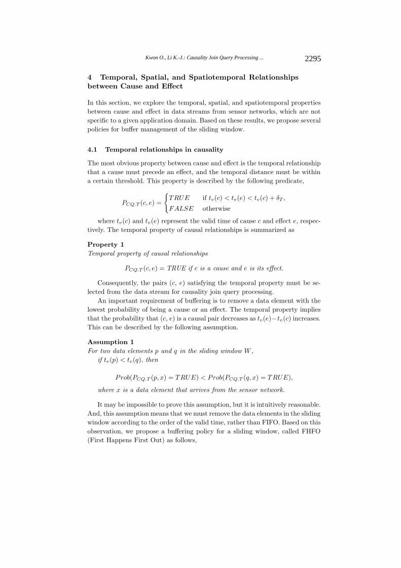
4.1 Temporal relationships in causality

The most obvious property between cause and effect is the temporal relationshipthat a cause must precede an effect, and the temporal distance must be withina certain threshold. This property is described by the following predicate,

PCQ.T (c, e) =

{TRUE if tv(c) < tv(e) < tv(c) + δT ,

FALSE otherwise

where tv(c) and tv(e) represent the valid time of cause c and effect e, respec-tively. The temporal property of causal relationships is summarized as

Property 1Temporal property of causal relationships

PCQ.T (c, e) = TRUE if c is a cause and e is its effect.

Consequently, the pairs (c, e) satisfying the temporal property must be se-lected from the data stream for causality join query processing.

An important requirement of buffering is to remove a data element with thelowest probability of being a cause or an effect. The temporal property impliesthat the probability that (c, e) is a causal pair decreases as tv(e)−tv(c) increases.This can be described by the following assumption.

Assumption 1For two data elements p and q in the sliding window W ,

if tv(p) < tv(q), then

Prob(PCQ.T (p, x) = TRUE) < Prob(PCQ.T (q, x) = TRUE),

where x is a data element that arrives from the sensor network.

It may be impossible to prove this assumption, but it is intuitively reasonable.And, this assumption means that we must remove the data elements in the slidingwindow according to the order of the valid time, rather than FIFO. Based on thisobservation, we propose a buffering policy for a sliding window, called FHFO(First Happens First Out) as follows,


p1p3p2p4p5p6

tttv

t

Window W

p3p2p4p5p6

t

Window W

p7

ti

titi+1

p3 p7c e

Missing result

Effect data Cause data


FIFO policyW = {p2, p3, p4, p5, p6} and size(W) > θmin(tt(p)) = p3 then delete p3

1912

178

1411

1210

134

1111

1912

178

1411

1210

134

2212

tttv

(a) FIFO buffering policy

p1p2p5p3p4p6

tttv

t

Window W

p2p5p3p4p6

t

Window W

p7

ti

titi+1

p3 p7c e



FHFO policyW = {p2, p3, p4, p5, p6} and size(W) > θmin(tv(p)) = p2 then delete p2

1912

178

1411

1210

134

1111

1912

178

1411

1210

134

2212

tttv

(b) FHFO buffering policy

Figure 4: Comparison of FIFO and FHFO

Definition 2. FHFO (First Happens First Out)The buffering policy FHFO for a sliding window W is defined as

FHFO(W ) : remove p ∈ W such that tv(p) = min({tv(q)|q ∈ W})

In comparison with FIFO, we reduce the omission of pairs, and consequentlyimprove the accuracy of the query results, as explained in figure 4.


In this example, we assume that the pair (p3, p7) is a causal pair. When anew data element p6 arrives, p3 is removed from the window according to theFIFO policy. When the next data element p7 arrives, p3 has been previouslyremoved, and consequently the pair (p3, p7) cannot be included in the result set.Compared with FIFO, p3 remains in the window, and p2 is removed from thewindow, since tv(p2) < tv(p3). This means that (p3, p7) may be included in thequery result.

4.2 Spatial Relationships in Causality

Spatial relationships between cause and effect are also an important property, aswell as temporal relationship. In general, spatial relationships are more compli-cated than temporal relationships, and expressed in several manners, includinggeometrical and topological relationships. However, in this paper, we focus ona general and obvious spatial relationship, in terms of the distance between thecause and effect.

PCQ.S(c, e) =

{TRUE if dist(p(c), p(e)) < δS ,

FALSE otherwise

p(c) and p(e) represent the locations of cause and effect, respectively. If theselocations are too distant, they cannot be a cause and its effect. Note that thedistance is defined according to the type of space and application.

The spatial property implies that the probability that (c, e) is a causal pairdecreases as dist(p(c), p(e)) increases, and it can be described by the followingassumption,

Assumption 2For two data elements p and q in the sliding window W,

if dist(p(p), p(x)) < dist(p(q), p(x)), then

Prob(PCQ.S(p, x) = TRUE) > Prob(PCQ.S(q, x) = TRUE),

where x is a data element that arrives from the sensor network.

While we can sort the data elements in W according to the valid time, wecannot sort them according the position. In order to apply this assumption tobuffering of a sliding window, we sort them according to the distance from DSMS.Although this distance may not fully reflect the spatial property for the bufferingpolicy, it could affect the sequence of the data stream. This spatial buffering pol-icy, viz. FCFO, involves removing the data element p with the smallest dist(p, b),where b is the location of DSMS. This policy is summarized as follows,


p3p1p4p2p5

t

Window W

ti


FCFO policyW = {p1, p2, p3, p4, p5} and size(W) > θmin(dist(p, b)) = p3 then delete p3

BS

dist(p1, b) = 4dist(p2, b) = 5

dist(p3, b) = 1

dist(p4, b) = 3

dist(p5, b) = 4

p1p4p5p2

t

Window W

ti

dist(p6, b) = 8p6

ti+1


p3

18104

16113

15101

1375

1083

tv18104

16113

15101

1375

1083

22158

ttd

tvttd

p1

p5p3

p2

p4

p6

Figure 5: Example of FCFO

Definition 3. FCFO (First Closely located First Out)The buffering policy FCFO, for a sliding window W , is defined as

FCFO(W ) : remove p ∈ W such that

dist(p, b) = min({dist(q, b)|q ∈ W}) or tcur − tt(p) > tmax.stay,

where tcur and tt(p) implies the current time and transactional time of p.

In this policy, we remove the data element if tcur − tt(p) > tmax.stay. Thisis to prevent the data element from remaining in the window indefinitely. Thismay happen when a data element arrives from a sensor very distant from b. If a

data element remains in the window longer than tmax.stay, then we remove thiselement. An example of this policy is explained in figure 5.

We suppose that sensors are located as shown in figure 5. When a new dataelement p5 arrives, then the data element that has remained longer than tmax.stay

is removed. If no data element remains longer than tmax.stay, then the dataelement with the smallest distance from DSMS, which is p3 in figure 5, is deletedfrom the window.

4.3 Spatiotemporal Relationships in Causality

The third relationship between cause and effect is the spatiotemporal one. Inthis paper, we only focus on the spatiotemporal relationship concerning the


p1p2p3p4p5

t

Window W

ti


FHCFO policyW = {p1, p2, p3, p4, p5} and size(W) > θIf tv(p)-tv(q) < tp+δP then

If min(dist(p, b)) = p1then delete p1

p2p3p4p5

t

Window W

ti

p6

ti+1


p1

p2p1 tv(p5)-tv(p1) = 3 < 4

tv(p5)-tv(p2) = 2 < 4

p2p1

dist(p1, b) < dist(p2,b)

104

113

61

75

83

tv 104

113

61

75

83

158d

tvd

Figure 6: Example of FHCFO

propagation speed. Assuming that the propagation speed is v and the distancebetween the cause and effect is s, then the effect occurs at least tp = s/v laterthan the cause. This relationship is expressed as the spatiotemporal predicatePCQ.ST (c, e)

PCQ.ST (c, e) =

{TRUE if tp < tv(e) − tv(c) < tp + δP ,

FALSE otherwise

In this relationship, δP represents the maximum tolerance of the propagationtime from the cause and effect. This means that the event cannot be the effectof the cause if it happens after a (tp + δP ) delay. Note that the spatiotemporalpredicate becomes a temporal predicate when tp=0.

Based on this result, we apply this relationship to the buffering policy. Sup-pose that a new data element x arrives at DSMS. A data element p in W may bethe cause of the subsequent data elements, if tv(p)− tv(x) < tp+δP . This meansthat p must remain in W until the propagation delay with the given tolerancehas expired. After the time has expired, the probability of a causal relationshipdecreases as time advances. Based on this result, we propose a buffering policyas follows,

Definition 4. FHCFO (First Happens and Closely located First Out)The buffering policy FHCFO for a sliding window W is defined as


FHCFO(W ) : If (tv(p) − tv(x) < tp + δP ), then

remove p ∈ W such that dist(p, b) = min({dist(q, b)|q ∈ W})Else

remove p ∈ W such that tv(p) = min({tv(q)|q ∈ W})

This policy is in fact a hybrid of FHFO and FCFO. An example of this policyis shown in figure 6.

In this example, we assume that tp + δP =4 and the sensors are located asshown in figure 5. When a new data element p5 arrives, we search p in W suchthat tv(p) − tv(p5) < tp + δP . Since every data element in W satisfies thiscondition, we select the data element with the minimum distance to DSMS. p1is then removed, because dist(p1, b) is the minimum.

5 Empirical Analysis

In this section, we present the results of experiments for analyzing and comparingthe proposed methods and FIFO.

5.1 Experiment Setup

In order to perform the experiments, we prepared a data set with the followingparameters.

• Spatial extent: [0, 1]2

• Location of DSMS: (0.5, 0.5)

• Number of sensors: 100

• Number of data elements per sensor: 1000

• Data detection period per sensor: randomly generated by an exponentialdistribution with a given expected value λ1

• Delay per hop: randomly generated by an exponential distribution with agiven expected value λ2

• Type of sliding window: tuple-based

• tmax.stay of the FCFO: nW × avg(� tt)


Table 1: Parameters and their experimental values

Parameter Description Range

λ1 Expected value of detecting period per sensor 0.1,0.15,...,0.5(sec)λ2 Expected delay per one hop 0.02,0.04,...,0.2(sec)tp Minimal propagation time from cause to effect 0.2,0.4,...,2.0(sec)δP Tolerance of tp 0.1,0.2,...,1.0(sec)nW Size of sliding window 50,100,...,500s Distance between cause and effect 0.2

We apply two exponential distributions using the expected value λ1 and λ2

respectively, to generate realistic transactional and valid time for sensor streams.There are generally two types of sliding window: tuple-based and time-based. Theobjective of the proposed buffering methods is to ensure that the data elementsthat satisfy the causality query remain within the limited window over the long-term. This problem is particularly important when the limited sliding windowover-flows. For this reason, we focus on the tuple-based sliding window ratherthan the time-based one. We set tmax.stay of FCFO as the time when the windowfills up. The parameters and their ranges are shown in table 1.

We measured the recall rate of the query results, to check the accuracy of theresults. In this paper, the recall rate is defined as the number of pairs selectedfrom the data stream with the proposed buffering policies over the number ofall pairs satisfying the causality predicates.

Recall(P ) = numResult(P )/numCausality

where P = {FIFO, FHFO, FCFO, FHCFO}

5.2 Results of experiments

We ran the experiments on Athlon 2.6GHZ Processor with 2.00GB RAM. Weperformed several experiments with the parameters in table 1, to check the accu-racy of each buffering policy. There are a number of combinations of parametervalues shown in table 1. We performed most experiments for the possible com-binations. But we only present the significant results in this paper, excludingresults where the accuracy was nearly 100% for every method.

5.2.1 Experiments on sliding window nW

Figure 7 shows the recall rate of each buffering policy with respect to the sizeof the sliding window nW in DSMS. The x- and y-axis represent the size of the


0

20

40

60

80

100

50 100 150 200 250 300 350 400 450 500

Rec

all

FIFOFHFOFCFOFHCFO

nW

1=0.1sec, 2=0.2sec, tp=0.4sec, δp=0.1sec, s=0.2

(a) λ2=0.2

0

20

40

60

80

100

50 100 150 200 250 300 350 400 450 500

Rec

all

nW


(b) λ2=0.1

Figure 7: Recall of four policies according to window size nW

sliding window nW and recall rate, respectively. It is obvious that the recall rateincreases as the window size increases. The experiments show that FHCFO isup to 5% better than FIFO, and FHFO is up to 4% better than FIFO. FHCFOhas an accuracy of up to 7% better than FIFO, especially with a small slidingwindow. This means that we must consider the spatiotemporal property of sensorstreams, to improve the accuracy of causality query processing in small devicewith limited memory, such as mobile devices.

When the expected delay is small (λ2 = 0.1, refer to figure 7(b)), the accuracyapproaches 100% with a small sliding window. This means that the probabilityof the reverse of sequence is low, if there is no long transfer delay. This is clearlyshown by figure 9. In this experiment, FHCFO also shows better accuracy thanFIFO, especially with a small window. One important result from this experi-


ment is that the size of the sliding window greatly affects the accuracy. When thesize of window is insufficient, more than half the results may be omitted. And,we observe that FCFO gives the worst accuracy in most of our experiments. Thismeans that we cannot improve the accuracy only via spatial considerations.

5.2.2 Experiments on detection period per sensor λ1

0

20

40

60

80

100

0.1 0.15 0.2 0.25 0.3 0.35 0.4 0.45 0.5

Rec

all

FIFOFHFOFCFOFHCFO

1(sec)

2=0.2sec, nW=300, tp=0.4sec, δp=0.1sec, s=0.2

(a) nW =300

0

20

40

60

80

100

0.1 0.15 0.2 0.25 0.3 0.35 0.4 0.45 0.5

Rec

all

FIFOFHFOFCFOFHCFO

1(sec)

2=0.2sec, nW=200, tp=0.4sec, δp=0.1sec, s=0.2

(b) nW =200

Figure 8: Recall of four policies according to detection period per sensor λ1

Figure 8 shows the recall rate for each buffering policy with respect to theexpected value of the detection period per sensor λ1. The x- and y-axis representthe detection period λ1 and recall rates, respectively. As the detection period


increases, the probability that the sequence of the data stream does not satisfythat of the occurrences decreases. Figure 8 shows that FHCFO is up to 4%better than FIFO with the large window (nW = 300, refer to figure 8(a)) and3% better with the small window (nW = 200, refer to figure 8(b)). FHFO isup to 3% better than FIFO as well. This is because FHCFO and FHFO controlthe buffer using the valid time of the stream data, to avoid the reverse sequenceof the stream. In the case that nW exceeds 450, the accuracy of each methodapproaches 100%, regardless of the detection period λ1.

5.2.3 Experiments on transfer delay per hop λ2

0

20

40

60

80

100

0.02 0.04 0.06 0.08 0.1 0.12 0.14 0.16 0.18 0.22(sec)

Rec

all

FIFOFHFOFCFOFHCFO

λ1=0.1sec, tp=0.4sec, δP=0.1sec, nW=300, s=0.2

(a) nW =300

0

20

40

60

80

100

0.02 0.04 0.06 0.08 0.1 0.12 0.14 0.16 0.18 0.2

Rec

all

FIFOFHFOFCFOFHCFO

2(sec)

λ1=0.1sec, tp=0.4sec, δP=0.1sec, nW=200, s=0.2

(b) nW =200

Figure 9: Recall of four policies according to transfer delay per hop λ2


Figure 9 shows the relationship between the recall rate of each bufferingpolicy and the delay per hop λ2. The x- and y-axis represent the delay per hopλ2 and recall rate, respectively. When the delay is short, the probability of thereverse sequence of the stream is also low, and consequently this gives a highaccuracy. In the case that the delay λ2 is long, where the probability of thereverse sequence of the stream is high, FHCFO is nearly 4% better than FIFOwith the large window (nW = 300, refer to figure 9(a)) and 7% better with thesmall window (nW = 200, refer to figure 9(b)). FHFO is also nearly 3% and 5%better than FIFO with the respective windows. FHCFO shows better accuracythan FHFO, because FHCFO includes spatial as well as temporal consideration.And, we found a significant reduction in accuracy with a small window size (referto figure 9(b)). This means that we must set a sufficiently large sliding windowto avoid omitting results.

5.2.4 Experiments on effect propagation time tp

Figure 10 shows the relationship between the recall rate and effect propagationtime between the cause and effect. The x- and y-axis represent effect propagationtime tp and recall rate, respectively The decrease of the recall rate according tothe increase of the propagation time is as we expect. However the reduction inaccuracy is significant when the delay is large (refer to figure 10(a)). This meansthat setting the size of the sliding window appropriately is very important toavoid omitting results. We can verify this in figure 10(b), where the size ofwindow is sufficiently large. The reduction in accuracy is slight when the size ofwindow is sufficiently large. When nW is sufficiently large, FHCFO is up to 5%better than FIFO, and FHFO is up to 4% better than FIFO.

5.2.5 Experiments on the effect propagation tolerance δP

Figure 11 shows the relationship between the recall rate and effect propagationtolerance δP . The x- and y-axis represent effect propagation tolerance δP andrecall rate, respectively. A high value of the effect propagation tolerance meansthat the difference between tv(cause) and tv(effect) is large. Then, the probabilitythat the cause and effect are in the buffer at the same time is low, as shown infigure 11. Both FHCFO and FHFO are up to 5% better than FIFO with asufficiently large window size, as shown in figure 11(b). However, FHFO doesnot give better accuracy than FIFO, especially when the size of window is notsufficiently large, as shown in figure 11(a) as well as figure 10(a). These resultsshow that maintaining a sufficiently large sliding window is very important forcontrolling the sensor stream data.


0

20

40

60

80

100

0.1 0.2 0.3 0.4 0.5 0.6 0.7 0.8 0.9 1tp(sec)

Rec

all

FIFOFHFOFCFOFHCFO

λ1=0.1sec, λ2=0.2sec, δP=0.1sec, nW=300, s=0.2

(a) nW = 300

0

20

40

60

80

100

0.1 0.2 0.3 0.4 0.5 0.6 0.7 0.8 0.9 1

Rec

all

tp(sec)

λ1=0.1sec, λ2=0.2sec, δP=0.1sec, nW=450, s=0.2

(b) nW = 450

Figure 10: Recall of four policies according to the effect propagation time tp

5.2.6 Experiments on CPU time

In order to perform causality query processing in sensor streams, only data ele-ments in the sliding window at the same time are valid . Therefore the processingtime of buffering methods is entirely related to the size of the sliding window.We measured the CPU processing time of each buffering method according tothe size of the window nW (refer to figure 12). The x- and y-axis represent thesize of the sliding window nW and CPU time, respectively. It is obvious that theCPU time increases as the size of window nW increases. The CPU time of FCFOFHCFO is larger than that of the others. This is because FCFO and FHCFOcalculate the distance between DSMS and each data element in the window,to test the spatial constraints of causality query processing. However, the CPU


0

20

40

60

80

100

0.1 0.2 0.3 0.4 0.5 0.6 0.7 0.8 0.9 1δP(sec)

Rec

all

FIFOFHFOFCFOFHCFO

λ1=0.1sec, λ2=0.2sec, tp=0.4sec, nW=300, s=0.2

(a) nW =300

0

20

40

60

80

100

0.1 0.2 0.3 0.4 0.5 0.6 0.7 0.8 0.9 1

Rec

all

FIFOFHFOFCFOFHCFO

δP(sec)

λ1=0.1sec, λ2=0.2sec, tP=0.4sec, nW=450, s=0.2

(b) nW =450

Figure 11: Recall of four policies according to the effect propagation toleranceδP

time is negligible, and has no effect on real-time causality query processing.In order to conclude the experiments, we summarize the important results

on the accuracy.

• The FHCFO policy consistently gives high accuracy causality join queryprocessing for data streams from sensors.

• The FHFO policy is better than FIFO in most cases, but not always.

• The FHCFO policy shows better performance than FHFO. This means thatwe must include both spatial and temporal considerations of a data stream,to deal with causality query processing.


0

0.1

0.2

0.3

0.4

0.5

0.6

50 100 150 200 250 300 350 400 450 500nW

CP

U ti

me(

10-3

sec)

FIFOFHFOFCFOFHCFO


Figure 12: CPU time of four policies according to the size of windownW

• In some cases, the accuracy falls below 50%. In order to guarantee reasonableaccuracy, the size of the sliding window must be sufficiently large. But theFHCFO policy guarantees more accurate results with a small sliding window.

• The FHCFO policy requires more CPU time than other buffering methods,but it is still negligible, thus causality query processing can occur in real-time.

6 Conclusion

Data streams collected from sensors contain a large volume of useful informa-tion including causal relationships. In this paper, we dealt with causality joinquery processing for data streams. To perform causality join query processingon sensor streams, it is important to study temporal, spatial, and spatiotempo-ral relationships between cause and effect in sensor streams. But the traditionalFIFO policy, which only considers the transactional time of the sensor data, isnot suitable for causality query processing, because of the limitations of the slid-ing window and delay. In this paper, we carefully examined the temporal, spatial,and spatiotemporal relationships, to satisfy causality join query processing, andproposed new buffering policies for the sliding window based on the results. Theintensive experimentation performed in our study shows that the proposed poli-cies are better than the traditional FIFO strategy. The contributions of our workare summarized as follows;


• Causality join query processing on sensor streams. Causality query process-ing can be used in various applications based on sensor networks.

• Definition of temporal, spatial, and spatiotemporal predicates. These pred-icates do not deal with transactional time, but rather the valid time of thesensor data, to clearly reflect the causal relationships between cause andeffect.

• Novel buffering policies based on temporal, spatial, and spatiotemporal con-siderations. The experiments show that the spatiotemporal buffering policyis better than FIFO.

Acknowledgements

This work was supported by the Brain Korea 21 Project, 2008, and the Ko-rean Land Spatialization project.

References

[Arasu et al. 03] Arasu, A., Babcock, B., Babu, S., Cieslewicz, J., Datar, M., Ito, K.,Motwani, R., Srivastava, U., Widom, J.: “Stream: The Standford Data Stream Man-agement System”; IEEE Data Engineering Bulletin 4, 1 (2003).

[Babcock et al. 02] Babcock, B., Babu, S., Datar, M., Motwani, R., Widom, J.: “Mod-

els and Issues in Data Stream Systems”; Proc. 2nd ACM SIGMOD-SIGACT-SIGART Symposium on Principles and Data Systems, ACM, NY (2002), 1-16.

[Chandrasekaran et al. 03] Chandrasekaran, S., Copper, O., Deshpande, A., Franklin,M. J., Joseph M, H., Hong, W., Krishnamurthy, S., Madden, S., Raman, V., Reiss,F., Shah, M.: “Telegraphcq: Continuous Dataflow Processing for an UncertainWorld”; Proc. of the Conference on Innovative Data Systems Research (2003), 11-18.

[Ding et al. 03] Ding, L., Rundensteiner, E. A., Heineman, G. T.: “MJoin: A Metadata-aware Stream Join Operator”; Proc. 2nd International Workshop on DistributedEvent-based Systems, ACM, NY (2003), 1-8.

[Freedman 04] Freedman, D. A.: “Graphical Models for Causation and the Identifica-tion Problem”; Evaluation Review 28, 4 (2004), 267-293.

[Gedik et al. 07] Gedik, B., Wu, K., Yu, P. S., Liu, L.: “GrubJoin: An Adaptive, Mul-tiway, Windowed Stream Join with Time Correlation-Aware CPU Load Shedding”;IEEE Transactions on Knowledge and Data Engineering 19, 10 (2007), 1363-1380.

[Golab and Ozsu 03] Golab, L., Ozsu, M. T.: “Issues in Data Stream Management”;ACM SIGMOD Record 32, 2 (2003), 5-14.

[Hammad et al. 03] Hammad, M. A., Aref, W. G., Elmagarmid, A. K.: “Stream Win-dow Join: Tracking Moving Objects in Sensor-network Databases”; Proc. 15th In-ternational Conference on Scientific and Statistical Database Management, IEEEComputer Society, Washington, D.C., USA (2003), 75-84.

[Holland 86] Holland, P. W.: “Statistics and Causal Inference”; Journal of the Ameri-can Statistical Association (1986).

[Khor et al. 05] Khor, I. J., Thomas, J., Jonyer, I.: “Sliding Window Protocol for Se-cure Group Communication in Ad-Hoc Networks”; Journal of Universal ComputerScience 11, 1 (2005), 37-55.


[Kun-Lung et al. 07] Wu, K., Yu, P. S., Gedik, B., Hildrum, K. W., Aggarwal, C.C., Bouillet, E., Fan, W., George, D. A., Gu, X., Luo, G., Wang, H.: “Challengesand Experience in Prototyping a Multi-Modal Stream Analytic and MonitoringApplication on System S”; Proc. 33th International Conference on Very Large DataBases, VLDB Endowment (2007), 1185-1195.

[Li et al. 05] Li, H., Lee, S., Shan, M.: “Online Mining Changes of Items over Con-tinuous Append-only and Dynamic Data Streams”; Journal of Universal ComputerScience 11, 8 (2005), 1411-1425.

[LTCCS 07] LTCCS (The Large Truck Crash Causation Study) (2007). http://www.loc.gov/marc/specifications/spechome.html.

[Madden and Franklin 02] Madden, S., Franklin, M. J.: “Fjording the Stream: An Ar-

chitecture for Queries over Streaming Sensor Data”; Proc. 18th International Confer-ence on Data Engineering, IEEE Computer Society, Washington, D.C., USA (2002),555-566.

[Mouratidis and Papadias 07] Mouratidis, K., Papadias, D.: “Continuous NearestNeighbor Queries over Sliding Windows”; IEEE Transactions on Knowledge andData Engineering 19, 6 (2007), 789-803.

[Mozer 99] Mozer, M. C.: “An Intelligent Environment Must Be Adaptive”; IEEE In-telligent Systems and Their Applications 14, 2 (1999) 11-13.

[Pearl 00] Pearl, J.: “Models, Reasoning and Inference”; Cambridge University Press(2000)

[Qin and Lee 03] Qin, X., Lee, W.: “Statistical Causality Analysis of INFOSEC AlertData”; Proc. 6th International Symposium on Recent Advances in Intrusion Detec-tion, LNCS 2820, Springer Berlin/Heidelberg (2003), 73-93.

[Silverstein et al. 00] Silverstein, C., Brin, S., Motwani, R., Ullman, J.: “Scalable Tech-niques for Mining Causal Structures”; Data Mining and Knowledge Discovery 4, 2-3(2000), 163-192.

[Tao and Papadias 06] Tao, Y., Papadias, D.: “Maintaining Sliding Window Skylineson Data Streams”; IEEE Transactions on Knowledge and Data Engineering 18, 3(2006), 377-391.

[Urhan and Franklin 00] Urhan, T., Franklin, M. J.: “XJoin: A Reactively-scheduledPipelined Join Operator”; IEEE Data Engineering Bulletin 23, 2 (2000), 27-33.

[Wu et al. 07] Wu, J., Tan, K., Zhou, Y.: “Window-oblivious Join: A Data-drivenMemory Management Scheme for Stream Join”; Proc. 19th International Confer-ence on Scientific and Statistical Database Management, IEEE Computer Society,Washington, D.C., USA (2007), 21-30.

[Wu et al. 09] Wu, J., Zhou, Y., Aberer, K., Tan, K.: “Towards Integrated and EfficientScientific Sensor Data Processing: A Database Approach”; Proc. 12th InternationalConference on Extending Database Technology: Advances in Database Technology,ACM, New York, USA (2009), 922-933.

[Zhou et al. 08] Zhou, Y., Aberer, K., Tan, K.: “Toward Massive Query Optimiza-tion in Large-Scale Distributed Stream Systems”; Proc. 9th ACM/IFIP/USENIXInternational Conference on Middleware, Springer-Verlag, New York, USA (2008),326-345.


Causality Join Query Processing for Data Streams via a

Documents

Transcript of Causality Join Query Processing for Data Streams via a