Causality - hsnamkoong.github.io

B9145: Reliable Statistical Learning Hongseok Namkoong

Causality

1

https://onlinelibrary.wiley.com/doi/abs/10.1111/ectj.12097

https://arxiv.org/pdf/1712.04912.pdfhttps://www.pnas.org/content/116/10/4156

https://scholar.harvard.edu/imbens/files/efficient_estimation_of_average_treatment_effects_using_the_estimated_propensity_score.pdf

https://www.cambridge.org/core/books/causal-inference-for-statistics-social-and-biomedical-sciences/71126BE90C58F1A431FE9B2DD07938AB

https://www.cambridge.org/core/books/causal-inference-for-statistics-social-and-biomedical-sciences/71126BE90C58F1A431FE9B2DD07938AB


Prediction and causality• A central goal of ML is to predict an outcome given

variables describing a situation- Given patient characteristics, will their outcome improve?

• Most decision-making problems revolve around a decision / intervention / treatment- What would happen if we changed the system?- Given patient characteristics, will their outcome improve if they

follow a new diet?

• We want to develop a scientific understanding of a decision

2


Prediction and causality

• Causal inference is a multi-disciplinary field built across economics, epidemiology, and statistics

• Focus is on questions about counterfactuals- What structure of data do we need to answer this question?- How do we interpret the key estimands?

• ML models can predict outcomes; when can it predict counterfactuals?- How can we leverage flexible ML models to infer causality?

3


Binary actions• Today we will focus on the setting with two actions

- One action represents treatment (1), the other is control (0)

• This is still foundational - Key difficulties still persist here despite the simplicity- Core technical insights will translate to more general settings

• In complex problems, this is often the de facto standard- Control is status quo, treatment is a new elaborate program- Throughout economics, medicine, and tech, it requires a

tremendous amount of domain knowledge and effort to come up with an alternative to the current system

4


Secret to life

5


Causality

6Figure credit: data science central

• You came up with a new diet regimen that you believe will alleviate symptoms of rheumatism (e.g. chronic joint pain)

• To test it, you recruit people to try the diet

• You find that- Small fraction on the diet experience chronic pain- Large fraction not on the diet (aka all rheumatism patients outside

your volunteer pool) experience chronic pain - Awesome! Everyone should try this diet

• But after years of adoption, you realize the diet does not affect chronic pain


Causality

7Figure credit: data science central

• What could have gone wrong?- Volunteers to the diet may have been people with healthy

predispositions, and affluent socioeconomic backgrounds

• Fundamental problem: we don’t observe counterfactuals

• How do we model this?

Potential outcomes

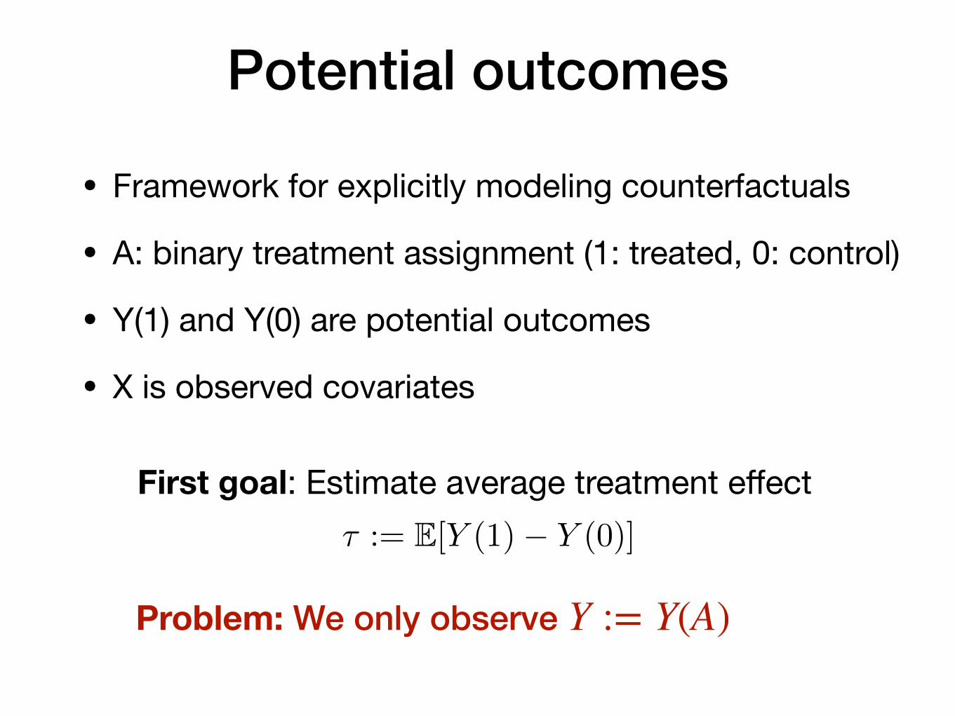
• Framework for explicitly modeling counterfactuals

• A: binary treatment assignment (1: treated, 0: control)

• Y(1) and Y(0) are potential outcomes

• X is observed covariates

Problem: We only observe Y := Y(A)

First goal: Estimate average treatment effect⌧ := E[Y (1)� Y (0)]

<latexit sha1_base64="MLmmO/wiUu/6elv3WpGWF57Pu1c=">AAACI3icbVDJSgNBFOxxjXEb9ZhLYxDiwTATBT0GRfAYwWxkhtDTeaONPYvdb4QQcvBjxKt+hzfx4sGP8A/sLAc1FjQUVfV4rytIpdDoOB/W3PzC4tJybiW/ura+sWlvbTd0kikOdZ7IRLUCpkGKGOooUEIrVcCiQEIzuD0b+c17UFok8RX2U/Ajdh2LUHCGRuraBQ9ZRr0ehHBHvfNOu+Tu0wPaLjn7ftcuOmVnDDpL3CkpkilqXfvL6yU8iyBGLpnWHddJ0R8whYJLGOa9TEPK+C27ho6hMYtA+4PxJ4Z0zyg9GibKvBjpWP05MWCR1v0oMMmI4Y3+643E/7xOhuGJPxBxmiHEfLIozCTFhI4aoT2hgKPsG8K4EuZWym+YYhxNb7+2aDStaRPQB5GJJnqYNx25fxuZJY1K2T0sVy6PitXTaVs5UiC7pERcckyq5ILUSJ1w8kCeyDN5sR6tV+vNep9E56zpzA75BevzG71Aoq0=</latexit>


ATE

9

• We only observe Y := Y(A)

• What could go wrong?- Volunteers to the diet (A = 1)

may have been people with healthy predispositions, and affluent socioeconomic backgrounds

First goal: Estimate average treatment effect⌧ := E[Y (1)� Y (0)]

<latexit sha1_base64="MLmmO/wiUu/6elv3WpGWF57Pu1c=">AAACI3icbVDJSgNBFOxxjXEb9ZhLYxDiwTATBT0GRfAYwWxkhtDTeaONPYvdb4QQcvBjxKt+hzfx4sGP8A/sLAc1FjQUVfV4rytIpdDoOB/W3PzC4tJybiW/ura+sWlvbTd0kikOdZ7IRLUCpkGKGOooUEIrVcCiQEIzuD0b+c17UFok8RX2U/Ajdh2LUHCGRuraBQ9ZRr0ehHBHvfNOu+Tu0wPaLjn7ftcuOmVnDDpL3CkpkilqXfvL6yU8iyBGLpnWHddJ0R8whYJLGOa9TEPK+C27ho6hMYtA+4PxJ4Z0zyg9GibKvBjpWP05MWCR1v0oMMmI4Y3+643E/7xOhuGJPxBxmiHEfLIozCTFhI4aoT2hgKPsG8K4EuZWym+YYhxNb7+2aDStaRPQB5GJJnqYNx25fxuZJY1K2T0sVy6PitXTaVs5UiC7pERcckyq5ILUSJ1w8kCeyDN5sR6tV+vNep9E56zpzA75BevzG71Aoq0=</latexit>

Person 5 Y(0) Y(1) Y(1) - Y(0)1 1 0 0 02 1 0 0 03 1 0 0 04 1 0 0 05 0 1 1 06 0 1 1 07 0 1 1 08 0 1 1 0


Randomized control trials

10

• First try: let’s randomize treatment assignments

• By virtue of randomized assignments, we have

• We can estimate final line from i.i.d. data

Y(1), Y(0) ⊥ A

τ = 𝔼[Y(1) − Y(0)] = 𝔼[Y(1) ∣ A = 1] − 𝔼[Y(0) ∣ A = 0]

= 𝔼[Y ∣ A = 1] − 𝔼[Y ∣ A = 0]

(Yi, Ai)

observable

also called A/B testing, (randomized) experiments



11



12


RCT with covariates

13

• If you have access to covariates X, and can estimate accurately, then we can improve this

• If by randomness more treatments get assigned to young patients with a better prognosis, then we will exaggerate the treatment effect- Problem goes away in large samples, but matters for small samples

• Using any regression model, we can estimate

- Random forests, boosted decision trees, kernels, NNs etc

𝔼[Y ∣ X, A]

𝔼[Y ∣ X, A = 1], 𝔼[Y ∣ X, A = 0] observable


Estimator

14


Fitting outcome models

15


CLT for covariate adjustments

16


Beyond RCTs

17

• What if clean randomization is not possible?

• Randomization sometimes affected by the site- Oxford / AstraZeneca trial made a dosage mistake at a location- Turned out to be more effective

• Ignoring variables that affect treatment assignment leads to biases


Beyond RCTs

18Slide by Ramesh Johari

• Run large-scale experiment, randomized for each sex

• vs - So maybe treatment is not effective?ℙ(Y = 1 ∣ A = 1) = 0.5 ℙ(Y = 1 ∣ A = 0) = 0.6

A

A


Simpson’s paradox


• But if you compute treatment effect for each sexes,

• So ATE = 0.1. What happened?

• Women are more likely to be in control than treatment; men are more likely to be in treatment than control. And women have higher potential outcomes on average than men.

𝔼[Y(1) − Y(0) ∣ X = m] = 𝔼[Y(1) − Y(0) ∣ X = w] = 0.1


Simpson’s paradox


• Issue here is that

• If you ignore sex as a confounding variable, you create a omitted variable bias in estimating the ATE

𝔼[Y(1) − Y(0)] ≠ 𝔼[Y(1) ∣ A = 1] − 𝔼[Y(0) ∣ A = 0]


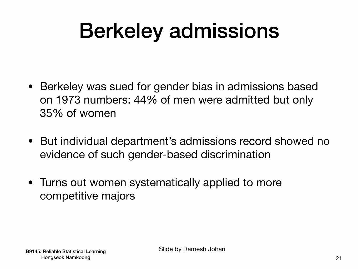
Berkeley admissions

• Berkeley was sued for gender bias in admissions based on 1973 numbers: 44% of men were admitted but only 35% of women

• But individual department’s admissions record showed no evidence of such gender-based discrimination

• Turns out women systematically applied to more competitive majors



Observational studies

22

• Randomization is sometimes infeasible or prohibitively expensive- e.g. post-market drug surveillance, effect of air pollution on long-

term health outcomes

• Experimentation can be risky in high-stakes scenarios- operational scenarios: new inventory system for Amazon, new

pricing algorithm for Uber

• May want to use existing large-scale data collected under some data-generating policy (e.g. legacy system)


No unobserved confounding

23

• Previous regression-based direct method still works if there are no unobserved confounders (also called ignorability)

Assumption.

• Observed treatment assignments are based on covariate information alone (+ random noise)- Treatment assignment does not use information about

counterfactuals

• Strong assumption. Often violated in practice.- e.g. doctors often use unrecorded info to prescribe treatments

Y(1), Y(0) ⊥ A ∣ X


No unobserved confounding

24


Overlap

25

• We need enough samples for both control and treatment throughout the covariate space- This governs the effective sample size

• Propensity score

• Assume that there exists such that almost surely

• This means I have at least number of samples for fitting the two outcome models

e⋆(X) := ℙ(A = 1 ∣ X)

ϵ > 0ϵ ≤ e⋆(X) ≤ 1 − ϵ

ϵn


Overlap

26

• This breaks if data is generated by a deterministic policy- e.g. always assign the drug (treatment) when age > 50

• We need sufficient amount of randomness in treatment assignment in all covariate regions

• Governs difficulty of estimation. Often violated in practice.


Direct method

27


Direct method

28


Inverse probability weighting• What if the outcome models are very complex and

difficult to estimate?

• A natural approach is to reweight samples, to change the distribution to - Essentially importance sampling

𝔼[ ⋅ ∣ A = 1,X] 𝔼[ ⋅ ∣ X]

29


Unbiasedness

30


CLT for IPW

31


Estimating propensity score

32


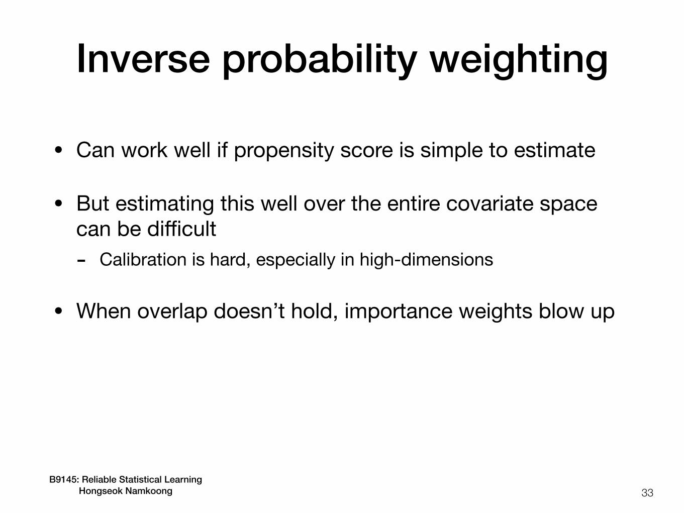
Inverse probability weighting

• Can work well if propensity score is simple to estimate

• But estimating this well over the entire covariate space can be difficult- Calibration is hard, especially in high-dimensions

• When overlap doesn’t hold, importance weights blow up

33


Augmented IPW• Can we combine the best of both worlds?

- Direct method + IPW

• Propensity weight residuals to debias the direct method

34


Unbiasedness

35


CLT for AIPW

36


Control variate

37


Control variate

38


Efficiency

39

• In fact, this is the best asymptotic variance we can get

• AIPW has optimal asymptotic variance, regardless of whether the propensity score is known or not

• Formalizing this requires a lot of work


Nuisance parameters

40

• If a good parametric model exists, then can estimate at the usual rates

• In general, these are infinite dimensional objects. Can be difficult to estimate.

1/ n


Semiparametrics

41

• We only care about estimating the ATE- One-dimensional estimand, infinite dimensional nuisance parameters

• Estimation accuracy of nuisance parameters is good only insofar as it helps with estimating the ATE

• Due to its high-dimensional nature, often difficult to estimate nuisances at parametric rates

• Goal: semiparametric estimators that are insensitive to errors in nuisance estimates


Doubly robust

42

• One main advantage of AIPW is that even if one of the nuisance parameter models are misspecified, you can still get correct asymptotic behavior


Doubly robust

43


Doubly robust

44


Orthogonality

45

• When is a semiparametric estimator insensitive to errors in nuisance estimates?

• Directional derivative of functional wrt nuisance parameters at true value is near-zero

• Ensures that a little perturbation in nuisance parameters near the truth values does not affect functional


Orthogonality

46


Orthogonality of AIPW

47


Orthogonality of AIPW

48


Why orthogonality?

49

• Allows getting central limit rates on ATE estimation even when we can only estimate nuisance parameters at slower rates

• In addition to no unobserved confounding, , we assume the following rate condition

• This allows us to trade-off errors between nuisance parameters. Only their product needs to go down at this rate!

e⋆(X), e(X) ∈ [ϵ,1 − ϵ]

∥ e − e⋆∥P,2(∥ μ1 − μ⋆1 ∥P,2 + ∥ μ0 − μ⋆

0 ∥P,2) = op(n−1/2)


Central limit result

50

• CLT for the semiparametric AIPW, even when nuisance estimates converge at slower-than-parametric rates

where

• This is the oracle asymptotic variance; when the true nuisance parameters are known

• AIPW achieves optimal asymptotic efficiency

n ( 1n

n

∑i=1

ψAIPW(Xi, Yi, Ai; μ0, μ1, e) − τ) ⇒ N(0,σ2AIPW)

σ2AIPW := Var (ψAIPW (X, Y, A; μ⋆

0 , μ⋆1 , e⋆))


Sketch of asymptotics

51


Sketch of asymptotics

52

Cro

ss-fi

tting

[Che

rnoz

huko

v '1

8]

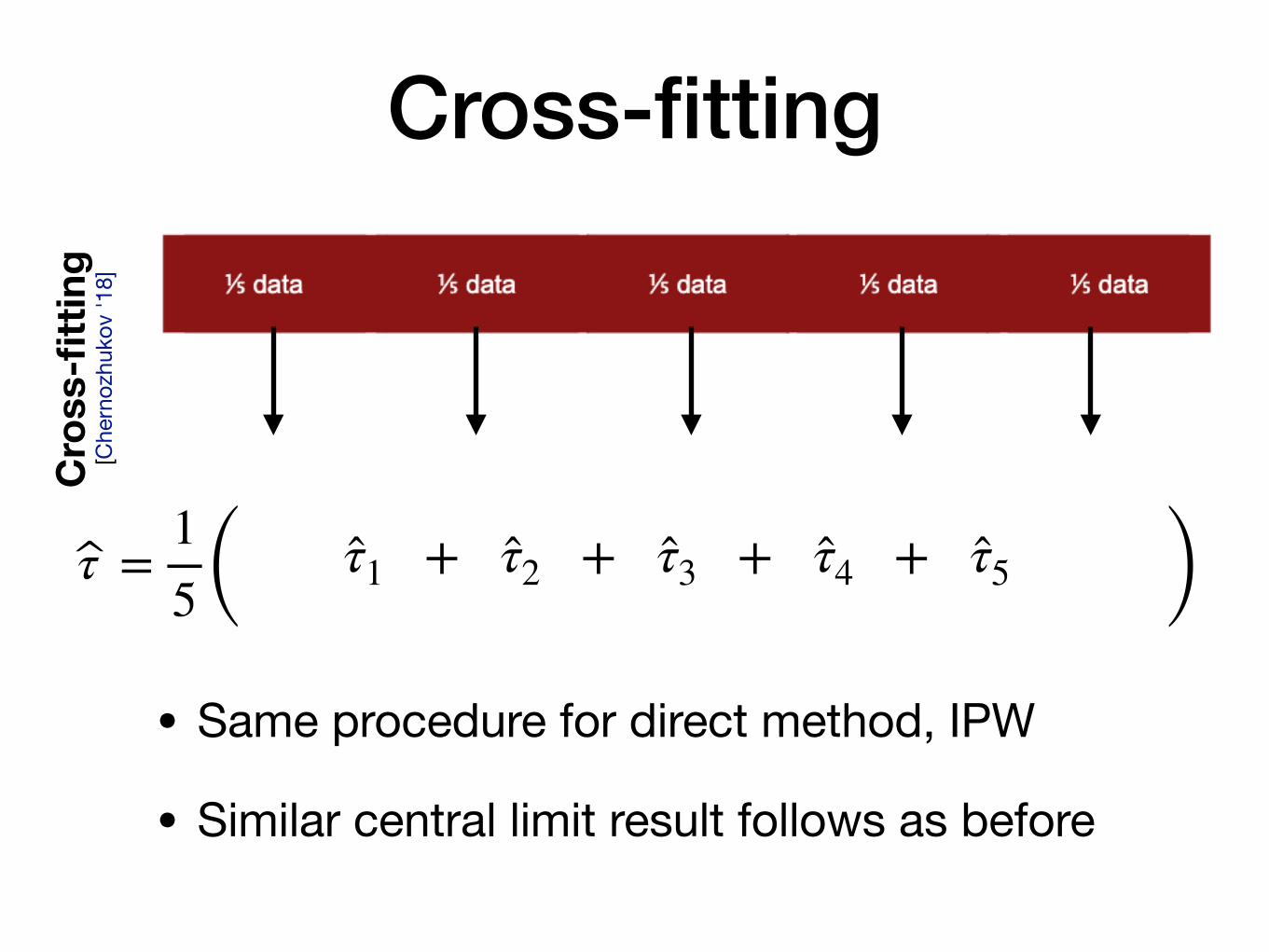
• Estimate nuisance parameters on the auxiliary sample

bµa(X) ⇡ E[Y (a) | X = x], a 2 {0, 1}

<latexit sha1_base64="sbl33p7RvlhWrMlbBwKJ4jXDkzI=">AAACQnicbVBNS1tBFJ1nWz9bjXXpZmgoRLDhPRFURBCs4FKh0UjmEe6bTMyQ+XjM3NcaHvG/+F8K3dZl/0JXilsXncQs6seBgTPnnMudOVmupMc4/hNNvXn7bnpmdm5+4f2HxaXK8sdTbwvHRYNbZV0zAy+UNKKBEpVo5k6AzpQ4y/oHI//su3BeWvMNB7lINVwY2ZUcMEjtyi770QMsmS6Gbag11yiDPHf2krLD1nkNwl3LDm3SPXqZrl8BZdJQVsbrNGHDdqUa1+Mx6EuSTEiVTHDcrtyyjuWFFga5Au9bSZxjWoJDyZUYzrPCixx4Hy5EK1ADWvi0HH9ySD8HpUO71oVjkI7V/ydK0N4PdBaSGrDnn3sj8TWvVWB3Oy2lyQsUhj8u6haKoqWjxmhHOsFRDQIB7mR4K+U9cMAx9Ppki8fQqg8B/0WHqPWjipLnhbwkpxv1ZLO+c7JZ3f86KWuWrJJPpEYSskX2yRE5Jg3CyTX5RX6Tm+hn9De6i+4fo1PRZGaFPEH08A+Ha69s</latexit>

be(X) ⇡ P(A = 1 | X)

<latexit sha1_base64="ff4lhMfrCUviHTiZTrpAYnc3lO8=">AAACK3icbVDLSgMxFM34tr6qLt0Eq1AXlhkR1IVQ0YXLCtYOdIaSSVMbmkyG5I5ahv6A/yK41d9wpbh17yeY1llY9UDgcM653JsTJYIbcN1XZ2Jyanpmdm6+sLC4tLxSXF27MirVlNWpEkr7ETFM8JjVgYNgfqIZkZFgjah3OvQbN0wbruJL6CcslOQ65h1OCVipVdwKbrsEMjYo+zs4IEmi1R0OauUTfIw9HEjexv5Oq1hyK+4I+C/xclJCOWqt4mfQVjSVLAYqiDFNz00gzIgGTgUbFILUsITQHrlmTUtjIpkJs9FvBnjbKm3cUdq+GPBI/TmREWlMX0Y2KQl0zW9vKP7nNVPoHIYZj5MUWEy/F3VSgUHhYTW4zTWjIPqWEKq5vRXTLtGEgi1wbIsBW5+xAbMrbVSZga3I+13IX3K1V/H2K0cX+6XqWV7WHNpAm6iMPHSAqugc1VAdUXSPHtETenYenBfnzXn/jk44+cw6GoPz8QXTP6al</latexit>

• Instead of sample-splitting, we can alternate the role of main and auxiliary samples over multiple splits

Cross-fitting

Cro

ss-fi

tting

[Che

rnoz

huko

v '1

8]

• Estimate ATE by plugging in nuisance estimates

τ1 :=1n

n

∑i=1

μ1(Xi) − μ0(Xi) +Ai

e(Xi)(Y − μ1(Xi)) −

1 − Ai

1 − e(Xi)(Y − μ0(Xi))

Cross-fitting

Cro

ss-fi

tting

[Che

rnoz

huko

v '1

8]

τ =15 ( )τ1 + τ2 + τ3 + τ4 + τ5

• Same procedure for direct method, IPW

• Similar central limit result follows as before

Cross-fitting


SUTVA

56

• Throughout we implicitly assumed there is only a single version of the treatment that gets applied to all treated units- This may not be true if drugs go stale in storage, or dosages differ

• We also assumed there is no interference between units - Whether or not individual i is treated has no impact on the treatment

effect of another individual j- This can also fail in many real-world scenarios

• Together these assumptions are called stable unit treatment value assumption (SUTVA)


Interference

57

• Any two-sided platform faces interference between units

• Consider the following scenario:- Lyft A/B tests a new promotion strategy for drivers- Each driver is randomized into treatment or control- It is observed that drivers finish a lot more rides with the promotion- So they decide this promotion is worth spending resources on

• But the estimate turned out to be an overestimate, not worth the cost of the promotion. Why?


Interference

58

• Both treated and control drivers see the same set of demand

• If promotion incentivizes treated drivers to work more for less nominal fares, this cannibalizes demand that would usually go to control drivers

• Interference occurs in a number of different settings- Two-sided platforms: Airbnb, ridesharing, ad auctions- Network effects: e.g. adoption of new education technology

• When this happens, the potential outcomes now depend on all possible treatment assignments- Very active area of research

2n


Assessing overlap

59

• “If the covariate distributions are similar, as they would be, in expectation, in the setting of a completely randomized experiment, there is less reason to be concerned about the sensitivity of estimates to the specific method chosen than if these distributions are substantially different.”

• “On the other hand, even if unconfoundedness holds, it may be that there are regions of the covariate space with relatively few treated units or relatively few control units, and, as a result, inferences for such regions rely largely on extrapolation and are therefore less credible than inferences for regions with substantial overlap in covariate distributions.”

• Imbens and Rubin


Assessing overlap

60

• Overlap governs effective sample size- Even approaches that don’t require propensity weighting is affected

under this fundamental restriction

• Causal inference literature has developed various “supplementary analysis” tools for assessing credibility of empirical claims

• One of the most common conventions is to plot the propensity scores of treated and control groups


Assessing overlap

61

• Difference in covariate distributions between treatment and control group is summarized by the propensity score

• Let be the density of in the treatment group (similarly )

• Let

f1(X) X f0(X)

p := ℙ(A = 1)

Var(e⋆(X)) = p(1 − p)(𝔼 [e⋆(X) ∣ A = 1] − 𝔼 [e⋆(X) ∣ A = 0])

= p2(1 − p)2 ⋅ 𝔼 ( f1(X) − f0(X)pf1(X) + (1 − p)f0(X) )

2


Assessing overlap

62

• A common visualization is to look at the pdf of the propensity score across treatment groups

• Plot approximates pdfs of the distribution

• For each , plot fraction of observations in the treatment group with (and similarly for control)

ℙ(e⋆(X) ∈ ⋅ ∣ A = a)

q ∈ (0,1)e⋆(x) = q


Assessing overlap

63

• Athey, Levin, Seira (2011) studied timber auctions- Award timber harvest contracts via first price sealed auction or open

ascending auction

• Idaho: randomized with different probabilities across different regions

• California: determined by small vs. large sales volume; cutoff varies by region


Idaho

64Slide by Susan Athey and Stefan Wager

Athey, Levin, Seira (2011)


California

65Slide by Susan Athey and Stefan Wager

Athey, Levin, Seira (2011)


Heterogeneous treatment effects

66

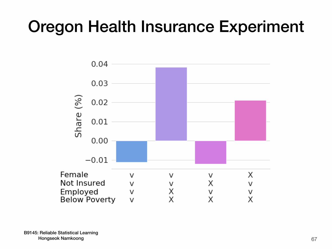
• Treatment effect often varies with user / patient / agent characteristics (covariates)

• Example: Oregon Health Insurance Experiment- Evaluate effect of Medicaid on low-income adults on emergency

department (ED) visits in 2008- Precursory study to federal Medicaid expansion in 2014, which cost

$553 billion/year- Insurance allows visits ED, but access to preventive care may also

reduce need of ED visits

B9145: Reliable Statistical Learning Hongseok Namkoong 67

Oregon Health Insurance Experiment

B9145: Reliable Statistical Learning Hongseok Namkoong 68

• Evaluate effect of wording on survey results (“welfare” vs “assistance to the poor”)

• Resoundingly positive treatment effects, but significant heterogeneity across covariates

Welfare attitudes experiment


CATE

• To estimate personalized treatment effects, we want to estimate the conditional average treatment effect (CATE)

• Few different ways to estimate this using black-box ML models

• Again, key challenging is missing data

- We never observed counterfactuals

τ(X) := 𝔼[Y(1) − Y(0) ∣ X]

69


S-Learner

70

• Shared feature representation, assuming similar model class for both treatment and control


T-Learner

71

• Can fit different models over treatment options


X-Learner

72

• Regress on the imputed treatment effect Y(1) - Y(0)

• Fit T-learner models and compute imputed treatment effects

if , if

• Fit another set of models on the two category of imputed values, take

Yi − μθ,0(Xi) Ai = 1 μθ,1(Xi) − Yi Ai = 0

τ1, τ0

τ(X) := e(X) τ0(X) + (1 − e(X)) τ1(X)

Kunzel et al. (2018)


X-Learner

73

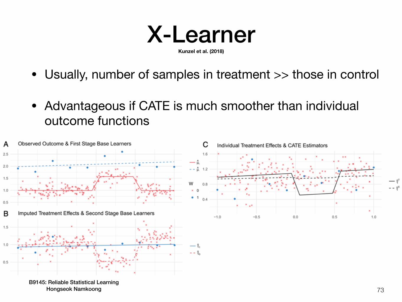
• Usually, number of samples in treatment >> those in control

• Advantageous if CATE is much smoother than individual outcome functions

Kunzel et al. (2018)


R-Learner

74

Nie and Wager (2020)


R-Learner

75

Nie and Wager (2020)

Causality - hsnamkoong.github.io

Documents

Transcript of Causality - hsnamkoong.github.io