CAT: High-Precision Acoustic Motion Tracking

Wenguang Mao, Jian He, and Lili QiuThe University of Texas at Austin

{wmao,jianhe,lili}@cs.utexas.edu

ABSTRACTVideo games, Virtual Reality (VR), Augmented Reality (AR), andSmart appliances (e.g., smart TVs) all call for a new way for usersto interact and control them. This paper develops high-preCisionAcoustic Tracker (CAT), which aims to replace a traditional mouseand let a user play games, interact with VR/AR headsets, and con-trol smart appliances by moving a smartphone in the air. Achievinghigh tracking accuracy is essential to provide enjoyable user expe-rience. To this end, we develop a novel system that uses audio sig-nals to achieve mm-level tracking accuracy. It lets multiple speak-ers transmit inaudible sounds at different frequencies. Based on thereceived sound, our system continuously estimates the distance andvelocity of the mobile with respect to the speakers to continuouslytrack it. At its heart lies a distributed Frequency Modulated Contin-uous Waveform (FMCW) that can accurately estimate the absolutedistance between a transmitter and a receiver that are separate andunsynchronized. We further develop an optimization framework tocombine FMCW estimation with Doppler shifts and Inertial Mea-surement Unit (IMU) measurements to enhance the accuracy, andefficiently solve the optimization problem. We implement two sys-tems: one on a desktop and another on a mobile phone. Our eval-uation and user study show that our system achieves high trackingaccuracy and ease of use using existing hardware.

CCS Concepts•Human-centered computing → Ubiquitous and mobile com-puting systems and tools; •Information systems → Mobile in-formation processing systems; •Hardware → Signal processingsystems;

KeywordsTracking; Acoustic signals; Doppler shift; FMCW; Optimization;Smartphone

1. INTRODUCTIONMotivation: Video games, Virtual Reality (VR), Augmented Re-ality (AR), and Smart appliances all call for a new way for users

Permission to make digital or hard copies of all or part of this work for personal orclassroom use is granted without fee provided that copies are not made or distributedfor profit or commercial advantage and that copies bear this notice and the full cita-tion on the first page. Copyrights for components of this work owned by others thanACMmust be honored. Abstracting with credit is permitted. To copy otherwise, or re-publish, to post on servers or to redistribute to lists, requires prior specific permissionand/or a fee. Request permissions from permissions@acm.org.MobiCom’16, October 03-07, 2016, New York City, NY, USAc© 2016 ACM. ISBN 978-1-4503-4226-1/16/10. . . $15.00DOI: http://dx.doi.org/10.1145/2973750.2973755

to interact and control them. For example, motion games (i.e.,the games played by movement) are popular across the world. Onthe other hand, through interviewing 100+ game players, we havefound many of them are unsatisfied with the existing tracking tech-nologies in the motion games: (i) they often complain about thetracking accuracy, and (ii) the coarse-grained tracking only sup-ports limited types of motion games, such as sports and dancinggames. However, many players prefer motion games that requiremore fine-grained movement, such as first person shooter (FPS).In addition, the current interfaces of VR/AR are rather constrained

(e.g., relying on tapping, swiping, or voice recognition). This sig-nificantly limits its potential applications. Moreover, smart appli-ances are becoming increasingly popular. For example, smart TVsoffer a rich set of controls and it is important for users to easilycontrol smart TVs. More and more appliances will become smart,and allow users to control them remotely.Since mobile devices, such as smartphones and smart watches,

are becoming powerful and ubiquitous, they can potentially serveas universal motion controllers. To turn a mobile device into aneffective motion controller, its movement should be tracked accu-rately - within a centimeter.There have been a number of very interesting work on motion

tracking and localization ( e.g., audio-based schemes [26, 30, 47,49], RF-based schemes [39, 41, 45, 46], and vision-based schemes[1, 2]). Recent works reduce the tracking error significantly byusing many antennas and new spectrum (e.g., 60 GHz). Despitesignificant work on localization and tracking, achieving mm-leveltracking on commodity devices remains an open challenge. There-fore, we aim to achieve high tracking accuracy, minimize error ac-cumulation over time, and remove the need of special hardware.

Our approach: In this paper, we develop a novel system, calledhigh-preCision Acoustic motion Tracker (CAT), which turns a mo-bile phone into a motion controller. CAT can be potentially usedto control game consoles, VR/AR, and smart appliances. A uniquefeature of our approach is that it uses existing hardware alreadyavailable, while achieving high accuracy and ease of use.We use audio signals for our tracking system because (i) it propa-

gates slowly, which makes it possible to achieve high accuracy, (ii)it can be supported by commodity devices thanks to widely avail-able speakers and microphones, and (iii) its processing cost is lowdue to its low sampling rate.In our system, the speakers serve as anchor points and play spe-

cially designed acoustic signals. Our system then estimates thedistances and velocities with respect to the speakers based on thereceived signals using a distributed Frequency Modulated Contin-uous Waveform (FMCW) and Doppler shifts. It then fuses the dis-tances and velocities in an optimization framework to accuratelytrack the movement.

Doppler shift is a well known phenomenon where the signal fre-quency changes as a sender or a receiver moves. By tracking theamount of frequency shift, we can estimate the speed of the mobilewith respect to the speakers. To determine its position, the speedneeds to be integrated over time, which incurs error accumulation.To minimize error accumulation, we develop a novel FMCW-

based approach to directly estimate the distance between the mo-bile and the speakers. Our FMCW differs from existing approachesdue to the distributed nature of our system: the speakers (i.e., trans-mitters) and the microphone on the mobile (i.e., receiver) are sepa-rate and unsynchronized. In this case, the transmission time, whichis required by traditional FMCW approaches, is not known by thereceiver. Our distributed FMCW addresses the issue using the fol-lowing steps: i) find a reference point and determine its absoluteposition, ii) estimate the distance change with respect to the refer-ence point when a mobile moves, 3) derive the absolute distancesbetween the current point and speakers. In this way, we no longerneed the transmission time. Moreover, a separate transmitter andreceiver have different sampling frequencies. To address the issue,we develop a simple procedure to calibrate and compensate for thefrequency offset.Furthermore, we develop an optimization framework to incorpo-

rate FMCW measurements and Doppler shifts over time for accu-rate tracking. These two types of measurements are complemen-tary: the former gives distance estimation, which does not incur er-ror accumulation, while the latter provides more accurate distancechange in a short term, which helps smooth the estimated trajec-tory. The framework can further incorporate IMU measurements(e.g., accelerometers and gyroscopes) to improve the accuracy.We implement our approach on two platforms: (i) one consisting

of a desktop and a smartphone, where the desktop processes the au-dio signals fed back from the smartphone to track the smartphone,and (ii) another consisting of just speakers and a smartphone, wherethe smartphone tracks its location in real time based on the receivedaudio signals. Our evaluation also uses different settings, which re-flect scenarios of console games and VR/AR. For 2D tracking, weshow that CAT can achieve median tracking error of 7 mm in a PC-like setup and 12 mm in a VR-like setup with two speakers. Thecorresponding errors under three speakers reduce to 5 mm and 7mm in 2D, respectively. For 3D, the error is 8 mm - 9 mm. In com-parison, our distributed FMCW alone has 2 cm error in 2D, and theDoppler alone [47] has 2 cm error in the first few seconds but itserror increases over time due to error accumulation (e.g., 8 cm after30 seconds in our experiments).Our major contributions include:

• a distributed FMCW approach that achieves highly accuratedistance estimation without requiring synchronized and co-locatedsender and receiver,

• an optimization framework to combine distance and velocityestimation over multiple time intervals to accurately track mo-tion, and an efficient algorithm to solve it on a mobile device,

• prototype systems that demonstrate 5-7mm error in 2D and 8-9mm error in 3D.

Paper outline: The rest of this paper is organized as follows. Wedescribe our approach in Section 2, and present implementationdetails in Section 3. We evaluate its performance in Section 4. Wereview related work in Section 5, and conclude in Section 6.

2. OUR APPROACHIn our system, multiple static speakers (e.g., those on TV, com-

puter, VR headset) transmit audio signals to a mobile. The mo-

bile continuously estimates its velocity (Section 2.1) and distance(Section 2.2) to the speakers, and uses an optimization frameworkto combine these estimates to track its location (Section 2.3). Wecan further incorporate the IMU measurements in our optimizationframework to improve the tracking accuracy (Section 2.4).

2.1 Estimating VelocityThe Doppler effect is a well known phenomenon where the fre-

quency of a signal changes as a sender or a receiver moves [23].Without loss of generality, we consider only the receiver moveswhile the sender remains static. The frequency changes with thevelocity as follows:

v =F s

Fc, (1)

where F is the original frequency of the signal, F s is the amount offrequency shift, v is the receiver’s speed towards the sender, and cis the propagation speed of sound waves. Therefore, by measuringthe amount of frequency shift F s, we can estimate the receiver’svelocity, which can further be used to get distance and location.We use the approach described in [47] to estimate the mobile’s

velocity as follows:

• Each speaker continuously emits sine waves at inaudible fre-quencies. Different speakers use different frequencies to distin-guish from each other.

• The mobile samples the received audio signals at 44.1 KHz (thestandard sampling rate), applies Hanning window to avoid fre-quency leakage, and then uses Short-term Fourier Transform(STFT) to extract frequencies. We use 1764 samples to com-pute STFT, which corresponds to the audio samples in 40 ms.Then, we find a peak frequency and compare it with the fre-quency of the original sine wave. The difference between thetwo is the frequency shift F s

• In order to enhance the accuracy, we let each speaker emit mul-tiple sine waves at different frequencies and let the mobile esti-mate the frequency shift at each of the frequencies and combinethese estimates by removing outliers and averaging the remain-ing estimates. We translate the final estimated frequency shiftto the velocity based on Formula 1.

2.2 Estimating Propagation Delay

2.2.1 MotivationAs shown in [47], the Doppler shift alone can be used to provide

reasonable tracking for a short time. However, since the Dopplershift gives a velocity estimate, it has to be integrated over time toget a distance estimate. Therefore, the error grows over time. Fortracking over a long time interval, the accuracy of the Doppler shiftbased tracking degrades. In fact, error accumulation is common inmany localization schemes (e.g., dead reckoning [33, 38]).This motivates us to develop a method to overcome the error

accumulation problem. One possibility is to directly estimate dis-tance between the speakers and the mobile based on the propaga-tion delay. Unlike velocity, which needs to be integrated over timeand suffers from error accumulation, distance measurements canbe used to directly determine the mobile’s location and have no er-ror accumulation. One way to estimate the propagation delay is tosend a pulse signal and compute the difference between transmis-sion time and arrival time. There are two practical challenges withthis simple approach: (i) Due to the time-frequency uncertaintyprinciple, we need large bandwidth in order to send a sharp pulsesignal with good time resolution. Otherwise, the arrival time esti-mate will be inaccurate. (ii) Even if we can perfectly detect the start

Figure 1: Chirp signals. Figure 2: Pseudo-transmitted signals.

20 40 60 80 100Index of the starting sample

0

0.5

1

Nor

mal

ized

cor

rela

tion

Figure 3: Correlation.

of the received signal, it is still challenging to estimate the propa-gation delay because (1) the sender and receiver’s clocks are notsynchronized and (2) there is non-negligible and variable process-ing delay at both ends; in commercial devices like smartphones, itis difficult to separate these delays from the propagation delay. Inthis section, we develop a new distributed FMCW based approachto address these challenges.

2.2.2 Traditional FMCWTo accurately estimate the propagation delay, instead of sending

a sharp pulse or pseudo-random sequence using large bandwidth[3, 49], we leverage a FMCW-based approach, which can achievehigh estimation accuracy with moderate bandwidth usage [3].FMCW approach lets each speaker transmit a chirp signal every

period. Figure 1 shows periodic chirp signals, whose frequencysweeps linearly from fmin to fmax in each period. The frequencywithin each sweep is f = fmin + Bt

T, where B is the signal

bandwidth, T is the sweep time. We integrate the frequency overtime to get the corresponding phase: u(t) = 2π(fmint + B t2

2T).

Therefore the transmitted signal during the n-th sweep is vt(t′) =cos(2πfmint

′ + πBt′2

T), where t′ = t− nT .

Consider a chirp signal propagates over the medium and arrivesat the receiver after a delay td. The received signal is attenuatedand delayed in time, and becomes:

vr = α cos(2πfmin(t′ − td) +

πB(t′ − td)2

T),

where α is the attenuation factor.The receiver mixes (i.e., multiplies) the received signal with the

transmitted signal. That is, vm(t) = vr(t)vt(t). Thus, vm(t) is aproduct of two cosines. By using cosA cosB = (cos(A − B) +cos(A + B))/2 and filtering out the high frequency componentcos(A+B), vm(t) becomes:

vm(t) = α cos(2πfmintd +πB(2t′td − t2d)

T). (2)

Suppose the mobile is at distance R from the speaker initially andmoves at a speed of v. Then td is given by (R + vt′)/c. Pluggingtd into Formula 2 gives us

α cos(2πfminR + vt′

c+ (

2πBt′(R + vt′)

cT− πB(R+ vt′)2

c2T)).

If we analyze the frequency components of the above signal bytaking the derivative of the phase, the constant term can be ignoredand the terms quadratic with respect to (1/c)2 are too small andcan also be ignored. The remaining frequency component, denotedas fp, becomes:

fp =1

2π

δPhase

δt′=

BR

cT+

fminv

c+

Bv

c,

since mean(t′) = T/2. When v is close to 0, there is a peak atBRcT

in the frequency spectrum. If there are multiple propagation

paths between the transmitter and the receiver, multiple peaks areobserved in the spectrum of the mixed signal. In this case, fp isdetermined by the first peak, which should correspond to the directpath. Based on measured fp, the distance R can be derived as:

R =fpcT

B. (3)

2.2.3 Our FMCWTraditional FMCW assumes that the transmitter and receiver are

co-located and share the same clock. However, in our system, thespeakers and microphone are separate and unsynchronized. Thus,we develop a distributed FMCW approach to support this situation.In our approach, we apply FMCW technique to derive the changeof distance to the speaker when the mobile moves from one posi-tion to another. Moreover, we propose a scheme to find a referencepoint and leverage this point to convert the distance change to theabsolute distance to the speaker. Also, we explicitly take into ac-count the impact of movement on FMCW to improve its accuracy.We further account for the impact of sampling frequency offset be-tween the speaker and microphone to get more accurate distanceestimation. Below we elaborate each of these techniques.Supporting a separate sender and receiver: In traditional FMCWtechnique, the transmitter and receiver have a shared clock. How-ever, in our setup the transmitter (i.e., speaker) and receiver (i.e.,microphone) are separate and have unsynchronized clocks. Precisesynchronization between the speaker and microphone in our sce-nario is challenging. Even a small synchronization error of 0.1 mswill lead to 0.1 ms×c ≈ 3.46 cm error, where c is the propagationspeed of sound and around 346 m/s.We estimate the propagation delay between a separate sender and

receiver as follows. First, we perform approximate synchroniza-tion on the received signals to ensure that every processing interval(when we fetch and process audio samples) is aligned with a sin-gle chirp signal, as shown in Figure 2, since FMCW requires analmost complete received chirp. Approximate synchronization canbe achieved by correlating the received signals with the originalchirp signal. The maximum correlation indicates the best align-ment. We select the time when the highest correlation peak is de-tected as the start time of the first processing interval. This synchro-nization only needs to be performed once at the beginning. After-wards, we fetch received signals every 40ms (our processing inter-val) for FMCW processing. Note that the synchronization is ap-proximate since the cross correlation usually shows multiple peakswith similar magnitude as shown in Figure 3.After synchronization, we need to mix a received signal in each

interval with a transmitted signal. However, the exact start time ofa transmitted signal is unknown to the receiver. So we introduce anotion of pseudo-transmission time, i.e., the time when the receiverassumes the transmission begins. Let t0 denote the difference be-tween the pseudo transmission time and actual transmission timeof the first chirp signal. t0 is an unknown constant to the receiver.At each interval, our estimated distance has a constant offset from

the actual distance due to t0. Since the offset is constant, we canestimate the distance change over time. To get an absolute distanceat any time, we need to know the absolute distance at some point(called a reference point) and use the distance change to get theabsolute distance at a new location.Based on the pseudo transmission time, the receiver can con-

struct a pseudo transmitted signal, which starts at that time, asshown in Figure 2. By mixing (i.e., multiplying) the received sig-nals with the pseudo transmitted signals and applying a similar pro-cedure as Section 2.2.2, we have:

Rn =cTfp

n

B+ ct0, (4)

where Rn is the distance between the transmitter and receiver dur-ing the n-th interval, fp

n is the peak frequency of the mixed signals,c is the propagation speed of the audio signal, T is the chirp dura-tion, and B is the bandwidth of the chirp signal, which is equal tofmax − fmin . Considering the above equations for two intervals,we can derive

Rn −R1 = (fpn − fp

1 )cT

B.

If the distance between the transmitter and the receiver in the firstinterval (denoted asR1) is known,Rn can be determined based on:

Rn = (fpn − fp

1 )cT

B+R1. (5)

Reference position estimation: To obtain the distance Rn, weneed to know the absolute distance between the speaker and mobileat some point (i.e.,R1), also called a reference point. One way is tomeasure using a ruler. This could be cumbersome and error-prone.We develop the following simple yet effective calibration schemeto quickly obtain a reference position.Consider there are two speakers. Without loss of generality, we

assume the two speakers are at (0, 0) and (A, 0), respectively. Welet a user move the mobile device back and forth parallel to thex-axis (i.e., the line connecting two speakers). As the mobile ismoving towards the speaker 2, it experiences a positive Dopplershift with respect to the speaker before reaching x = A and expe-riences a negative Doppler shift after departing from it. Therefore,we can detect the time when the Doppler shift changes its sign, andat that time the mobile moves to a point on x = A, which is ourreference point.Now we need to determine the distance between the reference

point and speakers: D1 and D2 in Figure 4. We can apply FMCWto estimate the difference between D1 and D2, denoted as ΔD,by having the two speakers transmit at the same time and adoptingthe same pseudo-transmission time. In this case, t0, the differencebetween the pseudo-transmission time and the actual transmissiontime, is the same for both speakers. Thus, by subtracting Formula 4for the two speakers, we have

ΔD = D1 −D2 =cT (fp,1 − fp,2)

B,

where fp,1 and fp,2 denote the peak frequencies detected by FMCWtechnique for the two speakers, respectively.BesidesD1−D2 = ΔD, we also know thatD2

1−D22 = A2 due

to the property of a rectangular triangle. Then we can determineD1

andD2 based on these equations. To improve the accuracy, we cansweep the mobile cross the reference position multiple times, anduse the mean as the estimation forD1 and D2.When there are three or more speakers, the mobile can choose

any position as the reference point. In this case, we can use themethod discussed above to determine ΔDij between speakers i

Figure 4: Estimating reference position.

and j. Based on these ΔD’s, we can solve the coordinate of thereference position, denoted as (x, y), by minimizing the followingobjective function:

(√

(x− x1)2 + (y − y1)2 −

√(x− x2)2 + (y − y2)2 −ΔD12)

2

+(√

(x− x1)2 + (y − y1)2 −

√(x− x3)2 + (y − y3)2 −ΔD13)

2

+(√

(x− x2)2 + (y − y2)2 −

√(x− x3)2 + (y − y3)2 −ΔD23)

2,

where (xi, yi) is the position of i-th speaker.Impact of movement: For clarity, we omit the impact of the re-ceiver’s movement when deriving Formula 5. But a non-negligiblevelocity will lead to an additional shift to the peak frequency of themixed signals. In this case, the peak frequency is at:

fpn =

B(Rn − ct0)

cT+

fminvnc

+Bvnc

, (6)

where vn is the receiver’s velocity with respect to the transmitter inthe n-th interval. For ease of explanation, we assume the receiveris static in the first interval. Thus, Rn becomes:

Rn = (fpn − fminvn

c− Bvn

c− fp

1 )cT

B+R1, (7)

According to the equation, the absolute distance Rn can be deter-mined by measuring the FMCW peak frequencies in the first andn-th interval (fp

n and fp1 ), the velocity during the n-th interval (vn)

based on the Doppler shift, and the reference distance (R1).

Figure 5: The frequency offset problem.

Frequency offset: Due to imperfect clocks, the sampling frequen-cies at the transmitter and receiver are not exactly the same [12].The frequency offset makes the sender and receiver experience dif-ferent time when sending or receiving the same number of sam-ples. This introduces an error in estimating the peak frequency ofthe mixed signals. Figure 5 shows an example to illustrate the is-sue, where a sender transmits a chirp consisting of 1764 samples.After a propagation delay (e.g., Delay 1), the chirp arrives at the re-ceiver. Since the receiver has a slightly different clock rate, it takesslightly longer for the receiver to accumulate these 1764 samples.Therefore, Delay 2 not only includes the propagation delay but alsothe difference between the transmission time and receive time forchirp 1 caused by different clock rates. Similarly, Delay 3 includesthe propagation delay and the difference between the transmissionand receive time for chirps 1 and 2. In general, if the sender andreceiver are static and their sampling frequency offset is constant,the estimated delay will increase linearly over time.

To compensate for this effect, we introduce a short calibrationphase at the beginning. We fix the receiver’s location during thecalibration. Without a sampling frequency offset, the peak fre-quency detected by FMCW should be fixed. The frequency offsetwill introduce a steady shift in the peak frequency over time. Wecan estimate the shift by plotting the peak frequency over time asshown in Figure 6. We then apply a least square fit to the measure-ment data. The slope of the line, denoted as k, captures how fastthe peak changes over time due to the frequency offset. Given theestimated slope, we process the raw measurements as follows:

fadjustedp = fraw

p − kt, (8)

where fadjustedp and fraw

p are the adjusted and raw peak frequen-cies, respectively, t is the time elapse from the start, and k is theslope of the fitted line. Figure 6(b) shows fadjusted

p is stable overtime after the compensation.

0 5 10 15 20Time (s)

125

130

135

140

145

Det

ecte

d FM

CW

peak

s (H

z)

Detected peaksFitted line

(a) Before compensation

0 5 10 15 20Time (s)

125

126

127

128

Det

ecte

d FM

CW

peak

s (H

z)

(b) After compensation

Figure 6: Estimating FMCW peak shift.

The sampling frequency offset may slowly change over time.Our experiments show that the initial estimation is valid for at leasta few minutes. We can further improve the accuracy over a longerduration by re-calibrating the frequency offset whenever the re-ceiver is stationary, which can be detected based on IMU.

2.3 Optimization FrameworkWe propose the following optimization framework that combines

the Doppler shift and FMCW measurements for accurate motiontracking. Specifically, we minimize the following function:

∑

i∈[k−n+1..k]

∑

j

α(|zi − cj | − |z0 − cj | − di,jFMCW )2+

∑

i∈[k−n+2..k]

∑

j

β(|zi − cj | − |zi−1 − cj | − vdoppleri−1,j T )2, (9)

where k is the current processing interval, n is the number of inter-vals used in the optimization, zi denotes the mobile’s position at thebeginning of the i-th interval, z0 denotes the reference position, cjdenotes the j-th speaker’s position, di,jFMCW denotes the distancechange from the reference location with respect to the j-th speakerat the i-th interval, vdoppleri,j denotes the velocity with respect to thej-th speaker during the i-th interval, T is the interval duration, andα and β are the relative weights of the measurement from FMCWand Doppler shifts.

The only unknowns in the optimization are the mobile’s positionover time (i.e., zi). The speakers’ coordinates cj can be determinedusing the method proposed by [47]. di,jFMCW and vdoppleri,j are de-rived from FMCW and Doppler shift measurement, respectively.Essentially, the objective reflects the goal of finding a solution zi

that best fits the FMCW and Doppler measurements. The first termcaptures the distance calculated based on the coordinates shouldmatch the distance estimated from the FMCW, and the second termcaptures the distance traveled over an interval computed from thecoordinates should match with the distance derived from the Dopplershift. Our objective consists of terms from multiple intervals toimprove the accuracy. The above formulation is general, and cansupport both 2-D and 3-D coordinates. zi and cj are both vectors,whose sizes are determined by the number of dimensions.This optimization problem is non-convex, which means that there

is no guarantee on convergence and the computation cost can behigh. To efficiently solve the problem, we develop an algorithmbased on convex optimization. The unknowns in the original opti-mization problem are the node’s coordinates over time. This yieldsa complicated objective involving √

.. To simplify the objective,we use the node’s distances to different speakers over time (de-noted as Di,j ) as unknowns (i.e., replacing |zi − cj | with Di,j inFormula 9), which is a convex function in terms ofDi,j . However,not all distances are feasible (i.e., there may not exist coordinatesthat satisfy the distance constraints). We need to derive additionalconstraints to enforce feasibility. In the first step, we solve a con-vex relaxation of the original problem by using the distances asthe unknowns and replacing feasibility constraints of the distanceswith triangular inequality constraints. Triangular inequality con-straints are necessary in order for the distances to be realizable in alow-dimensional Euclidean space. They are also sufficient to guar-antee feasibility in a 2D space, but not sufficient in a 3D space.Therefore, in the next step we project the solution obtained fromthe first step into a feasible solution space. This projection is re-lated to network embedding, which embeds network hosts into alow-dimensional space while preserving their pairwise distances asmuch as possible. We develop a embedding method based on Alter-nating Direction Method of Multipliers (ADMM) [4] to efficientlysolve the problem.Our optimization has following nice properties. First, it com-

bines FMCW with Doppler measurement, where the former givesdistance estimation without error accumulation while the latter pro-vides more accurate distance change in a short term. Effectivelycombining the two allows us to achieve high tracking accuracy.Second, it uses measurements from multiple time intervals to im-prove the accuracy. Third, we develop an efficient algorithm tosolve it. Fourth, other types of measurement can be easily incorpo-rated in the framework to enhance the accuracy, as shown below.

2.4 Leveraging IMU SensorsNext we leverage Inertial Measurement Unit (IMU) sensors along

with audio signals to improve the tracking accuracy by synchro-nizing measurements from IMU with the audio and adding theminto our optimization framework. Accelerometer is cheap in termsof hardware cost, processing overhead, and battery consumption.However, it is inaccurate for long-time tracking because double in-tegration is needed. To limit error accumulation, we first estimatethe initial velocity based on Doppler shifts and then integrate accel-erations over only a short time (e.g., 360 ms in our implementation)to get the distance traveled during this period. Moreover, we use thegyroscope to measure the rotation and translate the accelerometerreadings to the direction consistent to our tracking coordinate.We add additional terms to the optimization objective and new

optimization variables to incorporate the error with respect to theIMU sensors. Formula 10 shows the final objective. The first twoterms are the same as above. Let k denote the current interval. Thethird term reflects the difference between the distance traveled dur-ing the past n−1 intervals calculated based on the mobile’s coordi-nates versus the distance estimated from the initial velocity vinit

k−n+1

and IMU sensor readings, where vinitk−n+1 is the new optimization

variable and represents the initial velocity at the (k− n+ 1)-th in-terval. dIMU

k−n+1,k is the displacement from the start of (k−n+1)-th interval to the start of k-th interval, which is calculated basedon IMU sensor readings assuming the initial velocity is zero. Thefourth term reflects the difference between the average velocity inthe (k−n+1)-th interval estimated based on the IMU sensors ver-sus based on the Doppler shift, where vdoppleri is the velocity in thei-th interval estimated based on the Doppler shift and is a vector,and ΔvIMU

k−n+1 captures the velocity change in the (k − n + 1)-thinterval calculated based on IMU. σ and γ are the weights of thetwo new terms.

∑

i∈[k−n+1..k]

∑

j

α(|zi − cj | − |z0 − cj | − di,jFMCW )2+

∑

i∈[k−n+2..k]

∑

j

β(|zi − cj | − |zi−1 − cj | − vdoppleri−1,j T )2+

σ(zk − zk−n+1 − vinitk−n+1(n− 1)T − dIMU

k−n+1,k)2+

γ(vinitk−n+1 + 1/2 ·ΔvIMU

k−n+1 − vdopplerk−n+1 )2. (10)

2.5 SummaryPutting everything together, Procedure 1 shows the pseudo code

of our final system.

Algorithm 1 CAT tracking system1: Estimate speakers’ positions as in [47];2: Perform approximate synchronization to align the processing

intervals with the received chirps;3: Find a reference point;4: Estimate the peak shift rate due to sampling frequency offset;5: while TRUE do6: Fetch next 40 ms audio signals (1764 samples);7: Apply FFT to estimate Doppler shifts at various frequencies;8: Combine multiple Doppler shift estimates to derive velocity;9: Mix the received signals with the pseudo transmitted signals;10: Apply FFT on the mixed signals;11: Derive the distance based on peak frequency in the mixed

signal, peak shift rate, reference position, and velocity;12: Combine velocity and distance estimates (optionally with

IMU) to derive the coordinates based on optimization.13: end while

3. IMPLEMENTATIONWe implement CAT on two platforms. Our first platform consists

of a PC with speakers and an Android phone. The phone collectsaudio samples and inertial sensor data, and sends back to the PCthrough Android debug bridge. Our tracking program running onthe PC analyzes the collected measurements to track the phone inreal time. Our second platform consists of external speakers play-ing audio sound and a mobile phone analyzing the received audiosignal to track its location in real time. We use the first platform toperform all our evaluations and use the second platform to demon-strate the feasibility of running CAT on a smartphone.

Our system separately estimates Doppler shift and propagationdelay using sine waves and saw-shape chirp signals (as shown inFigure 1) on different frequency bands. Each Doppler measure-ment takes 1 KHz, which includes five sine waves at five differentfrequencies separated by 200 Hz to avoid mutual interference. Foreach FMCW measurement, the chirp signal with 2.5 KHz band-width is used. These signals are generated by Matlab and savedin a standard wav audio file, which can be played directly from ageneral-purpose speaker.We implement three different frequency allocations. The first

one is a two-speaker system for 2D tracking. We allocate 1 KHzfor each of the two speakers to continuously measure the Dopplershift. We allocate 2.5 KHz for FMCW estimation, and let twospeakers alternatively send chirp sequences to share that frequencyband. One speaker transmits chirps swiping from 17 KHz to 19.5KHz, while the other transmits chirps sweeping from 19.5 KHz to17 KHz. This helps to differentiate signals from different speakers.In addition. there is a 500 Hz guard band between the frequen-cies used for Doppler shift measurement and FMCW estimation.In this way, the audio signals in the two-speaker system occupy14.5-19.5 KHz, which are virtually inaudible to most people [15].Moreover, another benefit is that such frequency is not interferedby ambient sound. As reported in the measurements from [24], theambient interference is almost close to noise levels beyond 6KHzand becomes negligible beyond 8KHz. Note that when the speak-ers alternate sending chirps, for each interval we remove the errorterm associated with the silent speaker during that interval from theoptimization objectives (i.e., Formula 9 and 10).The second is a three-speaker system for 2D tracking to further

improve the accuracy. We let each speaker continuously send sinewaves for the Doppler shift estimation and chirp sequences for theFMCW measurement. In this case, each speaker occupies 4 KHzfrequency band (i.e., 1 KHz for Doppler, 2.5 KHz for FMCW, and0.5 KHz guard band). Including guard bands between speakers, theaudio signals altogether occupy 6.5 - 19.5 KHz, which is audible.As shown in Section 4, the accuracy of our two-speaker system iscomparable to that of the three-speaker system when the speakersare separated by 90 cm. When the separation reduces to 30 cm, thethree-speaker system becomes substantially better.The third is a four-speaker system for 3D tracking. In this case,

the first two speakers share a 2.5 KHz frequency band for FMCWmeasurement by alternatively sending chirp signals. Similarly, theother two speakers use another 2.5 KHz band for FMCW estima-tion. In addition, each speaker is allocated 1 KHz for Doppler shiftmeasurement. Thus, including the guard band, the audio signalsoccupy 9.5 KHz - 19.5KHz, which is audible.There are several ways of fitting the audio signals from three

or more speakers into inaudible band. One option is to let themalternate in sending chirp sequences and sine waves. Another op-tion is to use ultrasound speakers and microphones, which can sendand receive audio signals with frequencies higher than 20 KHz andhave much wider available bandwidth. A third option is to swapthe transmitters and receivers in our implementation, i.e., have themobile transmit and use the received signals by the microphonesconnected to PC for tracking. The new challenge is to get sepa-rate audio streams from individual microphones since many sys-tems output combined signals from all its microphones. We verifyit is feasible to use splitter and cable to get separate audio signalsfrom each microphone. In this way, we can simply use 4 KHz forboth the Doppler and FMCW estimation, which can easily fit intoinaudible spectrum supported by the existing hardware. We canfurther apply the techniques in [18] to smooth transitions and makethe sound even less audible.

4. EVALUATIONWe evaluate CAT using Dell XPS X9100 desktop with Intel i7

CPU and 8GB memory as a main processor. This desktop supportsat most 6 speakers. We use Logitech S120 2.0 speakers ($10 each).The speakers’ volume is set to 30 out of 100 to ensure it works in anormal range. We use Nexus 4 as our mobile device, which moveswithin 1m/s in our experiments.

Figure 7: Experiment setup.

For 2D tracking, we randomly move our hand with various speedsin a horizontal plane. We compare the tracking accuracy of CATwhen using 2 speakers versus 3 speakers. In addition, we alsocompare with the Doppler shift based approach using 2 speak-ers [47] and camera-based approach, the latter of which serves asthe ground truth. To facilitate the camera to get the ground truth,we put a blue marker on the phone and let the camera track theblue marker. Camera is not a general tracking solution becauseit requires good lighting condition, a visually distinct target, andline-of-sight. We ensure all these requirements are satisfied for thevision based tracking to work well.In our two-speaker system, the default separation between the

speakers is 0.9 m. In the three-speaker system, the third speaker S3is added as shown in Figure 7. The mobile device is 1.1 m awayfrom the line defined by the two speakers. Moreover, the micro-phone located at the bottom of the smartphone faces the speakers,as shown in Figure 8(a).For 3D tracking, we use four speakers. The placement of these

speakers are indicated by S1, S2, S4, and S5, as shown in Figure 7,where S4 (S5) is fixed at 0.7m above S1 (S2). Since it is difficultto get the precise ground truth location in 3D space with a cam-era, we conduct experiments for 3D tracking in the following way.We print the trajectory of a given shape (e.g., triangle or circle) ona paper, and attach the paper to a tilted surface. As the slope ofthe surface is known, the position of the trajectory in 3D space canbe determined. In the experiments, we move the smartphone fol-lowing the trajectory on the paper and use our scheme to track themovement in the 3D space. The tracking results are compared withthe printed trajectory to compute the tracking errors.

4.1 Micro BenchmarkFirst, we present micro benchmarks.

Estimating distance: In this experiment, the distance between thespeaker and the mobile is estimated based on Formula 7, assumingthe reference point (i.e.,R1) is known in advance. Figure 9(a) plotsthe estimated distance for a portion of our trace. As we can see, theestimated results closely follow the ground truth. The median erroris less than 4 mm, and 90-th percentile error is 9 mm.Figure 9(b) further plots the error in the distance estimation as

we vary the separation between the speaker and mobile, while thespeaker volume remains unchanged (30 out of 100). The estimation

(a) LOS

(b) NLOS case 3

Figure 8: Microphone orientation.

error increases when the separation is larger than 3 meters, andreaches 1 cm when the separation is 7 meters. Further increasingthe separation may lead to the failure of detecting FMCW peaks(i.e., fp

n in Formula 7). In this case, we need to increase the speakervolume to increase the operating range.

0 1 2 3 4Time (s)

1.05

1.1

1.15

1.2

Dis

tanc

e (m

)MeasuredGround truth

(a) Measured trace

1m 2m 3m 5m 7mSpeaker-mobile separation

0

0.5

1

Med

ian

erro

r (cm

)

(b) Estimation errors

Figure 9: The error of estimating distance.

We further evaluate the proposed scheme under no light-of-sight(LOS) between the speaker and microphone. First, we use a pieceof cloth to cover the microphone to emulate the mobile is in thepocket (case 1), and find the tracking error is 4.4 mm, similar tothat under LOS. In this case, the signals from all paths are atten-uated by a similar amount and we can detect the correct FMCWpeak and Doppler shift to accurately estimate the distance and ve-locity. Next, we put a small cardboard box (8 cm×5 cm×2 cm) atthe middle point of the line connecting the speaker and the micro-phone, while the active region of our speaker is 10 cm tall and 2cm wide (case 2). The tracking error increases to 5.9 mm, slightlyhigher than that under LOS. In this case, the direct path between thespeaker and microphone is blocked but the signal can arrive at themicrophone through a path close to the direct path. So our systemcan estimate the distance and velocity with a reasonable accuracy.Then we turn the mobile 90o away from the speaker (case 3), asshown in Figure 8(b). In this case, we can barely see the micro-

phone from the speaker. The tracking error becomes 5.1 mm due toa reason similar to case 2. Further increasing the cardboard size orturning the mobile away from the speaker will degrade the trackingaccuracy since both the direct path and nearby paths are blocked,which may cause an incorrect detection of FMCW peaks. As partof our future work, we plan to enhance the accuracy for these mostchallenging cases.Estimating the reference position: Next we evaluate the error inestimating the reference position. Each time when we swipe acrossthe speaker, we get one estimation of the reference position. Whenwe swipe multiple times, the reference point is estimated as theaverage across all sweeps. The more times we sweep, the more ac-curate the estimation is. We collect a trace from 969 swipes. Thenwe compute the average estimation error as we vary the number ofsweeps S and report the average across S sweeps. As shown in Fig-ure 10(a), the error bar is centered at the mean with the length set toits standard deviation of sampled mean. The error reduces consid-erably as we increase the number of sweeps from 1 to 2. It contin-ues to decrease until 4 sweeps. Afterwards, additional sweeps donot significantly reduce the error.

2 4 6 8 10Number of sweeps

0.5

1

1.5

2

2.5

Posi

tion

erro

r (cm

)

(a) Error in reference position

0 cm 0.5 cm 1 cm 2 cm 4 cmPosition error

0

0.2

0.4

0.6

0.8

Med

ian

erro

r (cm

)

(b) Impact of error

Figure 10: Results for estimating the reference position.

Figure 10(b) compares the median tracking error as we injecta varying amount of error to the reference position. We computethe trajectory error by shifting the entire trajectory by the error inthe reference position and computing the difference between theestimated and ground-truth trajectories. To compute the trajectorydifference, for each point on the estimated trajectory, we identifythe point on the ground-truth trajectory from the camera that hasthe closest timestamp, compute the Euclidean distance between thetwo points, and average over all points on the trajectory. Even with4 cm error in the reference position, we can still achieve around 7mm trajectory error, which demonstrates that the trajectory trackingis robust to the error in the reference position.Estimating FMCW peak shift: Figure 11 shows the estimatedpeak shift rate (due to the sampling frequency offset) as we in-crease the number of chirps used for estimation. As we can see, theestimation converges when we use 50 chirps, which take 2 s in ourimplementation, since the chirp duration is 40 ms.

4.2 2D Tracking AccuracyIn this section, we quantify the tracking accuracy by varying a

few parameters to understand their impacts. We compute the errorby comparing with the ground truth obtained from the camera.

0 20 40 60 80Number of chirps

0

1

2

3

Peak

shi

ft ra

te (H

z/s)

Figure 11: Estimating peak shift rate.

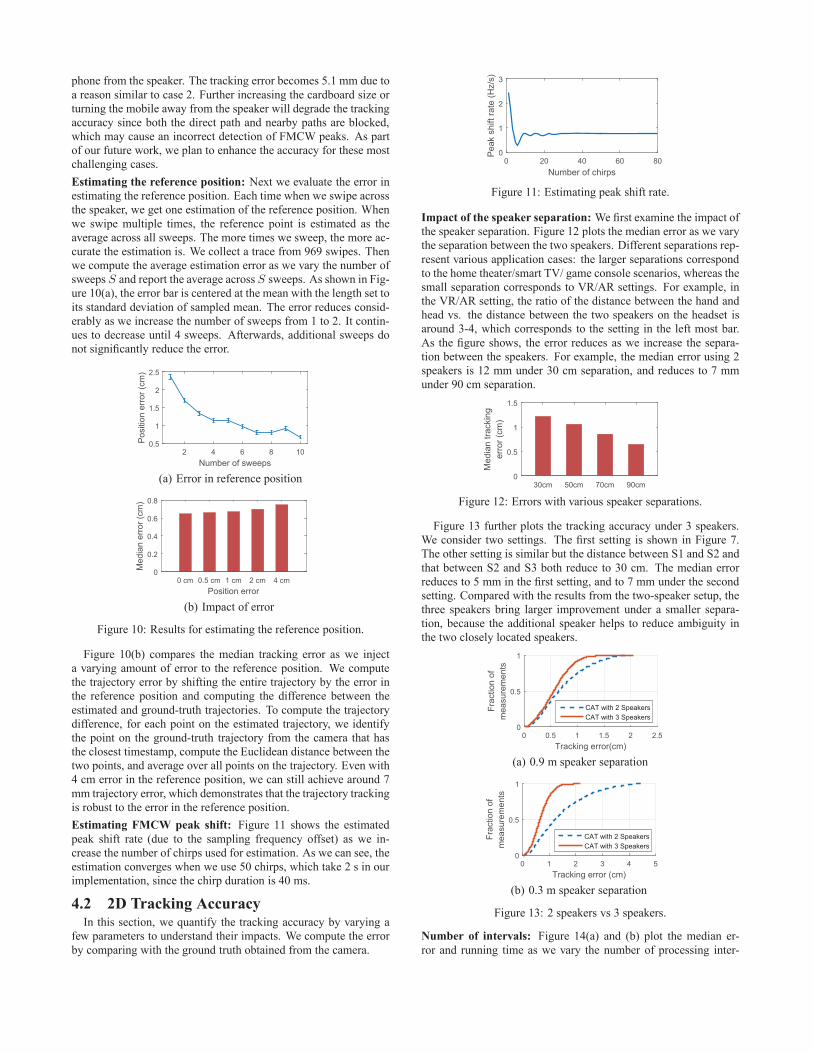
Impact of the speaker separation: We first examine the impact ofthe speaker separation. Figure 12 plots the median error as we varythe separation between the two speakers. Different separations rep-resent various application cases: the larger separations correspondto the home theater/smart TV/ game console scenarios, whereas thesmall separation corresponds to VR/AR settings. For example, inthe VR/AR setting, the ratio of the distance between the hand andhead vs. the distance between the two speakers on the headset isaround 3-4, which corresponds to the setting in the left most bar.As the figure shows, the error reduces as we increase the separa-tion between the speakers. For example, the median error using 2speakers is 12 mm under 30 cm separation, and reduces to 7 mmunder 90 cm separation.

30cm 50cm 70cm 90cm0

0.5

1

1.5

Med

ian

track

ing

erro

r (cm

)Figure 12: Errors with various speaker separations.

Figure 13 further plots the tracking accuracy under 3 speakers.We consider two settings. The first setting is shown in Figure 7.The other setting is similar but the distance between S1 and S2 andthat between S2 and S3 both reduce to 30 cm. The median errorreduces to 5 mm in the first setting, and to 7 mm under the secondsetting. Compared with the results from the two-speaker setup, thethree speakers bring larger improvement under a smaller separa-tion, because the additional speaker helps to reduce ambiguity inthe two closely located speakers.

0 0.5 1 1.5 2 2.5Tracking error(cm)

0

0.5

1

Frac

tion

ofm

easu

rem

ents

CAT with 2 SpeakersCAT with 3 Speakers

(a) 0.9 m speaker separation

0 1 2 3 4 5Tracking error (cm)

0

0.5

1

Frac

tion

ofm

easu

rem

ents

CAT with 2 SpeakersCAT with 3 Speakers

(b) 0.3 m speaker separation

Figure 13: 2 speakers vs 3 speakers.

Number of intervals: Figure 14(a) and (b) plot the median er-ror and running time as we vary the number of processing inter-

vals used in our optimization, respectively. The error bars in Fig-ure 14(b) are centered at the mean and the bar length reflects itsstandard deviation of sampled mean. For the running time, we com-pare two optimization solvers: 1) general non-linear solver NLopt[27] to optimize Formula 9 in Section 2.3; 2) embedding-basedsolver on the converted problem as proposed in Section 2.3. Thetwo solvers yield the same error, but the embedding is more effi-cient especially under a larger number of intervals. With 10 inter-vals (the default value in our evaluation), the optimization time is2 ms. In additional, it takes 2 ms to measure Doppler shift, and3 ms to measure FMCW. The total time to compute the position is8 ms, well below our processing interval 40 ms.

2 6 10 14 20Number of intervals

0

0.2

0.4

0.6

0.8

Med

ian

erro

r (cm

)

(a) Tracking Error

5 10 15 20Number of intervals

0

5

10

Run

ning

tim

e (m

s)

NLoptEmbed

(b) Running time

Figure 14: Number of intervals used in the optimization.

Impact of weights: We examine the impact of the weights (α, β)in our objective function (Formula 9 in Section 2.3). Figure 15 plotsthe CDF of errors under different weights. With weight (0,1), onlyDoppler shift is used in our scheme. This is essentially AAMouse[47]. With (1,0), only FMCW measurement is used and the op-timization becomes finding the intersection of circles whose sizesare the distance estimates from FMCW. The other weights all useboth Doppler and FMCW. As we would expect, the tracking errorof using both information is significantly lower than using one ofthem. The weight (1,40) performs the best because it makes thetwo terms (after multiplying the weights) in our optimization ob-jective have similar magnitude. However, the tracking error is notsensitive to the exact weights: a wide range of weights offer similarperformance, as shown in the figure.

0 5 10 15 20Tracking error(cm)

0

0.5

1

Frac

tion

ofm

easu

rem

ents

AAMouseFMCW-onlyCAT (1,1)CAT (1,40)CAT (1,1000)

Figure 15: Varying the weights.

Leveraging the sensors: Figure 16 plots the median errors withor without using IMU sensors in our two-speaker tracking system.As it shows, using IMU sensors is beneficial to improve the track-ing performance. When two speakers are separated by 90 cm, the

tracking error is reduced by 3%. When the separation between thespeakers decreases to 30 cm, using IMU reduces the tracking errorby 6%. We expect the benefit of incorporating IMU increases asthe accuracy of IMU improves. Moreover, our optimization frame-work is flexible to leverage other types of measurements to furtherimprove the performance.

30 cm 90 cm0

0.5

1

Med

ian

track

ing

erro

r (cm

)

w/o IMUwith IMU

Figure 16: Comparison between with and without IMU.

4.3 3D Tracking AccuracyIn this section, we evaluate CAT with four speakers in 3D space.

3D tracking performance: In this experiment, we evaluate thetracking performance for drawing a triangle and a circle in the 3Dspace. In Figure 17, the graphs on the left show the trajectoriestracked by CAT versus the ground truth, and the graphs on theright show the corresponding tracking errors. As we can observe,the median error for 3D tracking is about 8 mm - 9 mm, whichis slightly larger than those in 2D experiments because of largerdegree of freedom.

0

0.1

0.6 1.05

z-co

ordi

nate

(m)

1

x-coordinate (m) y-coordinate (m)

0.2

0.950.4 0.90.85

CATGround Truth

(a) Trajectory

0 1 2 3Tracking error(cm)

0

0.2

0.4

0.6

0.8

1

Frac

tion

of m

easu

rem

ents

(b) Error

0

0.1

0.6 1.05

z-co

ordi

nate

(m)

1

x-coordinate (m) y-coordinate (m)

0.2

0.950.4 0.90.85

CATGround Truth

(c) Trajectory

0 1 2 3Tracking error(cm)

0

0.2

0.4

0.6

0.8

1

Frac

tion

of m

easu

rem

ents

(d) Error

Figure 17: 3D tracking accuracy.

Error accumulation: To check if our scheme has error accumu-lation, we compare the tracking errors for drawing triangles in 3Dspace with AAMouse [47] (using four speakers). The experimentlasts for 180 s. During this period, we keep moving the smartphonefollowing the printed triangle trajectory. As shown in Figure 18,the 3D tracking error of CAT is stable over time, and significantlyout-performs AAMouse. This demonstrates our method effectivelyaddresses error accumulation problem.Robustness to ambient sound: To evaluate the robustness of ourscheme to ambient sound, we continuously play music when using

0 50 100 150time (s)

0

5

10

15

Trac

king

erro

r (cm

)

CATAAMouse

Figure 18: Error over time.

CAT to track the smartphone. We play several different genres ofmusic (e.g., Jazz, Pop, and Classic) together to emulate differentambient sound. The speaker for playing music is placed near S1 asshown in Figure 7. The music volume is the same as the acousticsignals for tracking. Figure 19 compares the tracking error withand without playing music. We observe no significant differencebetween two cases, which indicates that our scheme is robust toambient sound.

0 1 2 3Tracking error(cm)

0

0.5

1

Frac

tion

ofm

easu

rem

ents

w/o musicw music

Figure 19: Impact of ambient sound

4.4 User StudyWe recruit 10 users and report evaluation results from our user

study. We conduct two types of experiments. In the first experi-ment, we let users touch targets shown on a screen and measure thedistance traveled. A shorter distance indicates more accurate track-ing and easier to use. In the second experiment, users are askedto draw some shapes on the screen and we compare the measuredtrajectories versus the original trajectories to quantify the accuracy.We use our 2D tracking systems for user study.In the evaluation, we run each experiment 10 times involving

different users. Each user has 10-minute training for each scheme(i.e., CAT and AAMouse). When using CAT, the users are asked tohold the device in such a way to avoid their hands blocking the mi-crophone. The overall experiment lasts about 1 hour for each user.The distances of our ground truth trajectories used for pointing anddrawing experiments are 41.37 cm for pointing, 73.26 cm for draw-ing a triangle, 60.67 cm for drawing a double-circle, and 153.1 cmfor drawing a loop back, as shown in Figure 23. The tracking andvisualization are both done online in real-time. Meanwhile, we alsostore the complete traces to compute various performance metricsoffline. For touching point, we compare the distance traveled inorder to touch a target, which reflects the amount of user effort.For drawing shapes, we measure the error by comparing the actualpointer trajectory with the ground-truth trajectory.Target pointing evaluation: We evaluate the usability of CAT asa pointing device based on the distance traveled in order to touchseveral targets. We let a user start from a middle point in a line,move to the right end, and then come back to the left end.Figure 20 shows the average distance traveled by our scheme and

AAMouse, which is a Doppler shift-based method. As a reference,we plot the exact path length to touch these points. We consider apointer touches the target if it is within 10 pixels (around 1.38 cm)of the target. As another reference, we also plot the minimum pos-sible trace length, which corresponds to the exact distance - 2×1.38= 41.37 - 2.76 = 38.62 cm. CAT with two or three speakers (labeled

CAT 3S CAT 2S AAMouse 2S38

39

40

41

42

43

44

Trac

e le

ngth

(cm

)

Length using CAT/AAMouseExact lengthMinimum possible length

Figure 20: Target pointing evaluation.

by “CAT 2S” and “CAT 3S”, respectively in the figure) both havesmaller distance than the Doppler shift based approach. We expectthe gap between CAT and Doppler based scheme will increase asthe number of points to touch increases due to error accumulationin the latter.Figure 21 plots the trajectories that correspond to the median per-

formance for each scheme. Even though the distances traveled byboth schemes do not differ significantly, there is a clear differencebetween their trajectories. CAT closely follows the ideal trajectory.The trajectory of CAT under 3 speakers (not shown) is even better.In comparison, even though the Doppler based scheme is alreadyclose to the ideal trajectory, there is still clear deviation.

-15 -10 -5 0 5 10 15X(cm)

-10

-5

0

5

10

Y(cm

)

(a) CAT (2 speakers)

-15 -10 -5 0 5 10 15X(cm)

-10

-5

0

5

10

Y(cm

)

(b) AAMouse (2 speakers)

Figure 21: Trajectories for pointing target.

Drawing evaluation: Next we ask a user to draw simple shapes:a double-circle, triangle, and loop back, shown on the screen us-ing the pointer controlled by CAT or AAMouse [47]. We measurethe quality of the drawings by calculating the distance between thedrawn figure and the original shape. For each point in the originalfigure, we calculate its distance to the closest point in the drawing,and average across all points. While this does not perfectly cap-ture the quality of the drawing, it provides reasonable distinctionbetween well-drawn and poorly-drawn figures.Figure 22 shows the CDF of the drawing error. CAT yields signif-

icantly lower error than AAMouse. For example, the median errorfor drawing loop back with CAT are 3.8 mm (3 speakers), 4.3 mm(2 speakers), while that for Doppler-based tracking is 11.2 mm. Itis interesting to see that the tracking errors in user study are usuallysmaller than those presented in Section 4.2. This is because that inthe user study users can adjust their movement when they see thetrajectory deviate from the ground-truth.Figure 23 further plots trajectories drawn by the two schemes

corresponding to the median error. As before, it is evident that

0 1 2 3 4Tracking error (cm)

0

0.5

1

Frac

tion

ofm

easu

rem

ent

CAT 3SCAT 2SAAMouse 2S

(a) Double circle

0 1 2 3 4Tracking error (cm)

0

0.5

1

Frac

tion

ofm

easu

rem

ent

CAT 3SCAT 2SAAMouse 2S

(b) Triangle

0 2 4 6Tracking error (cm)

0

0.5

1

Frac

tion

ofm

easu

rem

ent

CAT 3SCAT 2SAAMouse 2S

(c) Loop back

Figure 22: CDF of drawing error.

CAT consistently follows the original shapes much closer than theDoppler based scheme.

-20 -10 0 10 20X(cm)

0

10

20

Y(cm

)

(a) CAT

-20 -10 0 10 20X(cm)

0

10

20

Y(cm

)

(b) AAMouse

-20 -10 0 10 20X(cm)

0

5

10

15

20

Y(cm

)

(c) CAT

-20 -10 0 10 20X(cm)

0

5

10

15

20

Y(cm

)

(d) AAMouse

-20 -10 0 10 20X(cm)

0

5

10

15

20

Y(cm

)

(e) CAT

-20 -10 0 10 20X(cm)

0

10

20

Y(cm

)

(f) AAMouse

Figure 23: Patterns drawn by CAT (2 speakers) and AAMouse (2speakers) corresponding to the median error.

Mobile phone implementation:We also implement CAT on a mo-bile phone (Nexus 4). The phone uses CAT to efficiently track itsown location using fast signal processing in [22] and the optimiza-tion solving algorithm mentioned in Section 2.3. The total timerequired to process audio samples and determine the position is 31ms, lower than our processing interval (40ms). The CPU usage isaround 35%. The tracking accuracy of the mobile phone is the sameas that of the desktop version, because the only difference betweenthe two versions is where the signal processing and computationare performed.We make the phone running CAT to serve as a motion controller

for video games, including Crossy Road [43] and Fruit Ninja [35]by mapping the phone’s movement into a cursor movement in gamesusing Windows API mouse_event. We ask 5 users to use our mo-tion controller to play these games, and they find the performanceis comparable to a traditional mouse.

5. RELATED WORKWe classify the related work based on the types of the signals

and underlying techniques used for tracking and localization.

Audio based schemes: Audio signals are attractive for localizationand tracking due to its slow propagation speed, which improvesaccuracy. Cricket [34] uses a combination of RF and ultrasound,and achieves a median error of 12 cm with 6 beacon nodes. Com-pared with Cricket, CAT improves the accuracy, and removes theneed of dense deployment and special hardware. [30] develops anovel scheme that can estimate the propagation delay by havingboth ends send and receive audio signals to cancel out the process-ing time and clock difference. Based on [30], [49] develops a se-ries of system approaches to make accurate distance ranging formobile gaming. Similar to [30], [49] relies on cross-correlation todetermine the propagation delay. To achieve high accuracy, 10-16KHz bandwidth is used in [49]. In comparison, FMCW can achievemore accurate estimation of propagation delay using more narrowbandwidth (e.g., 2.5 KHz). FingerIO [26] develops a novel device-free tracking scheme to track a moving finger near a smartphoneor a smartwatch. CAT differs from FingerIO in that it is a devicebased tracking and works for a larger distance (e.g., a few meters),but faces synchronization problem that does not exist in device-free tracking. AAMouse [47] is closest to this paper. Differentfrom [47], we estimate the distance using a new FMCW-based ap-proach in addition to velocity measurement and fuse the two usingan effective optimization framework to enhance the accuracy andminimize error accumulation.RF-based schemes: RF has been widely used for localization andtracking. ArrayTrack [45] is a pioneering fine-grained tracking sys-tem based on WiFi by using an array of antennas. It achieves a me-dian error of 23 cm using 16 antennas. RF-IDraw [39] achieveshigh resolution and low ambiguity by placing 8 RFID antennaswith different spacing. Its median error is 3.7 cm. WiDraw [36]enables hand-free drawing in the air by estimating angle of arrival(AoA) based on CSI. Its median error is within 5 cm when using 25WiFi transmitters. mTrack [41] achieves high tracking accuracy byleveraging the phase of 60 GHz RF signals as well as sophisticatedhardware (e.g., highly directional and steerable 60 GHz antennas).Tagoram [46] uses commercial off-the-shelf RFID for localizationand tracking. When the target moves along an unknown track (as inour context), the median error is 12 cm. In comparison, our systemcan run on commodity hardware and achieve higher accuracy.Other sensor based schemes: IMU sensors can also be used formotion tracking. However, its tracking error accumulates rapidlyover time due to noisy measurements and the need of double in-tegration [47]. Kinect [1] uses depth sensors and Wii [2] uses in-frared cameras to track movement. They both require line-of-sightand have limited accuracy. LeapMotion [19] uses sophisticated vi-sion techniques to recognize a wide range of gestures. Comparedwith the vision based techniques, audio-based approaches are gen-erally more efficient and flexible: its signal processing cost is lowand it works under different lighting conditions and often withoutline-of-sight (e.g., under small obstacles since there exists a detourpath close to the direct one or obstacles that do not significantlyattenuate the audio signal, such as cloth and paper).

FMCW-based schemes: FMCW based technique has been usedfor localization and motion tracking. Most existing schemes useco-located transmitter and receiver sharing the same clock. Forexample, [3] applies RF FMCW signals to 3D device-free trackingand achieves the tracking error of 10-20 cm. [25] leverages acousticFMCW to detect chest and abdomen movements, which is used toidentify sleep apnea.FMCW has also been applied to the systems with separate trans-

mitters and receivers. Such systems tend to have larger range andstronger SNR. However, most of these systems assume strict timesynchronization between the transmitter and the receiver withoutstudying how to achieve synchronization (e.g., [10, 17, 21]). [40,42] study synchronization for distributed FMCW systems. GPSsignals have been considered for synchronization, which is veryexpensive. In general, synchronization significantly complicatesthe design and implementation of a distributed system. Therefore,we use relative distance change and reference point localization toavoid the need of synchronization.There are a couple of schemes that do not need synchronization.

In [7, 44], a separate transmitter and receiver use FMCW to trackanother moving target. In this case, chirp signals arrive at the re-ceiver via two paths: the direct path from the transmitter to the re-ceiver, and the reflected path from the transmitter to the target andfinally reaching the receiver. FMCW is used to estimate the differ-ence between the propagation delay of the two paths. The length ofthe reflected path via the target is determined based on the lengthof the direct path, which is assumed to be known. When multiplereceivers exist, the target’s position can be estimated based on thelength of reflected paths to different receivers. In our scenario, thetarget to be tracked is the receiver itself and the above scheme isnot applicable. [6, 14] develop FMCW to measure the time differ-ence of arrival (TDOA) from different transmitters to the receiver.Since such methods give the difference between the distances todifferent anchors, they require more anchor nodes than the numberof dimensions for localization, whereas our approach derives ab-solute distance from each anchor and the number of anchor nodesrequired is equal to the number of dimensions. [11] measures theround-trip time by letting one node send and another node respondupon receiving the signals. This approach may lead to significanterrors in many systems, including smartphones, since they cannotprecisely control the transmission time or determine the exact re-ceiving time. Moreover, since the scheme in [11] requires bothnodes to send, receive, and process signals whereas our approachonly requires a node to either transmit or receive and process thesignals, our approach is more widely applicable.Some radars use a triangular chirp based FMCW for joint dis-

tance and velocity estimation [31], where the chirp frequency in-creases over time in the first half and then decreases in the secondhalf. The first and second halves of the received chirp signal ex-perience different frequency shifts. When we observe two peakfrequencies in the spectrum of the mixed signal, we can derive dis-tance based on the average of the two frequencies and derive ve-locity based on their difference. However, when the chirp durationis short, the frequency domain resolution is limited and two peaksmay merge together, which makes the joint estimation impossible.Based on our experiments, we find that two peaks will merge to-gether when the chirp is within 200 ms, and become fully separatedwhen the chirp is longer than 1 s. Such a long chirp duration is notacceptable for tracking, since it leads to significant processing de-lay. Therefore, joint estimation is not applicable to our context.Moreover, our distributed FMCW and optimization framework aregeneral, and can support different waveforms, including the trian-gular waveform.

Gesture recognition: The goal of gesture recognition is to deter-mine which gesture best matches the current measurement. Henceit requires training data collected from pre-defined gestures. IMUsensors are widely used for gesture recognition [5, 16, 20, 29].They can also be combined with other measurements, such as EMGsensors [48] and ultrasound [28], to further improve the perfor-mance. WiSee [32] proposes a novel device-free gesture recog-nition based on WiFi signals. [8, 9, 13, 37] use the Doppler shiftof the audio signal for gesture recognition. In general, continuoustracking is more challenging due to the lack of training data or pat-terns to match against.

6. CONCLUSIONThis paper presents a novel tracking system. At its core is a

new distributed FMCW-based distance estimation that (i) supportsa separate sender and receiver, (ii) localizes a reference point totranslate the relative distance to the absolute distance at new lo-cations, (iii) explicitly takes into account the additional frequencyshift caused by the movement, and (iv) takes into account the sam-pling frequency offset between the sender and receiver. We furthercombine FMCWwith the Doppler shift and IMU sensors over mul-tiple time intervals to continuously track the mobile. Our evalua-tion shows that CAT achieves mm-level accuracy and ease of useusing existing hardware. Our future work includes further enhanc-ing the robustness of our tracking system for a wide range of usagescenarios including varying degrees of multipath, and developingapplications that leverage such capabilities.

7. ACKNOWLEDGEMENTSThis work is supported in part by NSF Grants IIP-1546831, CNS-

1343383, and Cisco gift funding.

8. REFERENCES[1] Microsoft X-box Kinect. http://xbox.com.[2] Nintendo Wii. http://www.nintendo.com/wii.[3] F. Adib, Z. Kabelac, D. Katabi, and R. Miller. WiTrack:

motion tracking via radio reflections off the body. In Proc. ofNSDI, 2014.

[4] Augmented lagrangian method. http://en.wikipedia.org/wiki/Augmented_Lagrangian_method.

[5] S. Agrawal, I. Constandache, S. Gaonkar, R. Roy Choudhury,K. Caves, and F. DeRuyter. Using mobile phones to write inair. In Proc. of ACM MobiSys, pages 15–28, 2011.

[6] B. Al-Qudsi, M. El-Shennawy, Y. Wu, N. Joram, andF. Ellinger. A hybrid TDoA/RSSI model for mitigatingNLOS errors in FMCW based indoor positioning systems. InProc. of IEEE 11th Ph. D. Research in Microelectronics andElectronics (PRIME), pages 93–96, 2015.

[7] M. Ash, M. Ritchie, K. Chetty, and P. V. Brennan. A newmultistatic FMCW radar architecture by over-the-airderamping. IEEE Sensors Journal, 15(12):7045–7053, 2015.

[8] M. T. I. Aumi, S. Gupta, M. Goel, E. Larson, and S. Patel.Doplink: Using the Doppler effect for multi-deviceinteraction. In Proc. of ACM UbiComp, 2013.

[9] K.-Y. Chen, D. Ashbrook, M. Goel, S.-H. Lee, and S. Patel.Airlink: Sharing files between multiple devices using in-airgestures. In Proc. of ACM Ubicomp, 2014.

[10] T. Derham, S. Doughty, K. Woodbridge, and C. Baker.Design and evaluation of a low-cost multistatic netted radarsystem. IET Radar, Sonar & Navigation, 1(5):362–368,2007.

[11] R. Gierlich, J. Hüttner, A. Dabek, and M. Huemer.Performance analysis of FMCW synchronization techniquesfor indoor radiolocation. In Proc. of European Conference onWireless Technologies, pages 24–27, 2007.

[12] S. Gollakota and D. Katabi. Zigzag decoding: Combatinghidden terminals in wireless networks. In Proc. of ACMSIGCOMM, 2008.

[13] S. Gupta, D. Morris, S. Patel, and D. Tan. Soundwave: usingthe Doppler effect to sense gestures. In Proc. of the ACMCHI, pages 1911–1914, 2012.

[14] Y. Huang, P. V. Brennan, and A. Seeds. Active RFID locationsystem based on time-difference measurement using a linearFM chirp tag signal. In Proc. of IEEE Personal, Indoor, andMobile Radio Communications (PIMRC), pages 1–5, 2008.

[15] P. G. Kannan, S. P. Venkatagiri, M. C. Chan, A. L. Ananda,and L.-S. Peh. Low cost crowd counting using audio tones.In Proc. of the 10th ACM Conference on Embedded NetworkSensor Systems, pages 155–168, 2012.

[16] J.-H. Kim, N. D. Thang, and T.-S. Kim. 3-d hand motiontracking and gesture recognition using a data glove. In 2009IEEE International Symposium on Industrial Electronics,pages 1013–1018, 2009.

[17] K. Kulpa. Continuous wave radars–monostatic, multistaticand network. In Advances in Sensing with securityapplications, pages 215–242. Springer, 2006.

[18] P. Lazik and A. Rowe. Indoor pseudo-ranging of mobiledevices using ultrasonic chirps. In Proc. of Sensys, 2012.

[19] Leap motion. https://www.leapmotion.com/.[20] J. Liu, L. Zhong, J. Wickramasuriya, and V. Vasudevan.

uWave: Accelerometer-based personalized gesturerecognition and its applications. Pervasive and MobileComputing, 5(6):657–675, 2009.

[21] Y. Liu, Y. Kai, R. Wang, O. Loffeld, X. Wang, et al. Modeland signal processing of bistatic frequency modulatedcontinuous wave synthetic aperture radar. IET Radar, Sonar& Navigation, 6(6):472–482, 2012.

[22] W. Mao and L. Qiu. Efficient implementation ofsynchronization and FFT for mobile. http://www.cs.utexas.edu/~wmao/ReferenceLink/CATEff.pdf.

[23] R. A. Meyers. Encyclopedia of physical science andtechnology. Facts on File, 1987.

[24] R. Nandakumar, K. K. Chintalapudi, V. Padmanabhan, andR. Venkatesan. Dhwani: Secure peer-to-peer acoustic NFC.In Proc. of ACM SIGCOMM, 2013.

[25] R. Nandakumar, S. Gollakota, and N. Watson. Contactlesssleep apnea detection on smartphones. In Proc. of ACMMobiSys, 2015.

[26] R. Nandakumar, V. Iyer, D. Tan, and S. Gollakota. FingerIO:Using active sonar for fine-grained finger tracking. In Proc.of ACM CHI, pages 1515–1525, 2016.

[27] NLopt. http://ab-initio.mit.edu/wiki/index.php/Main_Page.[28] G. Ogris, T. Stiefmeier, H. Junker, P. Lukowicz, and

G. Troster. Using ultrasonic hand tracking to augmentmotion analysis based recognition of manipulative gestures.In Proc. of 9th IEEE International Symposium on WearableComputers (ISWC), pages 152–159, 2005.

[29] T. Park, J. Lee, I. Hwang, C. Yoo, L. Nachman, and J. Song.E-gesture: a collaborative architecture for energy-efficientgesture recognition with hand-worn sensor and mobiledevices. In Proc. of ACM SenSys, pages 260–273, 2011.

[30] C. Peng, G. Shen, Y. Zhang, Y. Li, and K. Tan. BeepBeep: a

high accuracy acoustic ranging system using COTS mobiledevices. In Proc. of ACM SenSys, 2007.

[31] D. Pierrottet, F. Amzajerdian, L. Petway, B. Barnes,G. Lockard, and M. Rubio. Linear FMCW laser radar forprecision range and vector velocity measurements. In MRSProc., volume 1076, pages 1076–K04. Cambridge Univ.Press, 2008.

[32] Q. Pu, S. Gupta, S. Gollakota, and S. Patel. Whole-homegesture recognition using wireless signals. In Proc. of ACMMobiCom, 2013.

[33] H. Rashid and A. K. Turuk. Dead reckoning localisationtechnique for mobile wireless sensor networks. IET WirelessSensor Systems, 2015.

[34] A. Smith, H. Balakrishnan, M. Goraczko, and N. Priyantha.Tracking moving devices with the Cricket location system.In Proc. of ACM MobiSys, 2005.

[35] H. Studios. Fruit ninja. http://fruitninja.com/.[36] L. Sun, S. Sen, D. Koutsonikolas, and K. Kim. WiDraw:

enabling hands-free drawing in the air on commodity WiFidevices. In Proc. of ACM MobiCom, 2015.

[37] Z. Sun, A. Purohit, R. Bose, and P. Zhang. Spartacus:spatially-aware interaction for mobile devices throughenergy-efficient audio sensing. In Proc. of ACM Mobisys,pages 263–276, 2013.

[38] H.-J. von der Hardt, D. Wolf, and R. Husson. The deadreckoning localization system of the wheeled mobile robotromane. In Proc. of IEEE/SICE/RSJ InternationalConference on Multisensor Fusion and Integration forIntelligent System, 1996.

[39] J. Wang, D. Vasisht, and D. Katabi. RF-IDraw: virtual touchscreen in the air using RF signals. In Proc. of ACMSIGCOMM, 2014.

[40] W.-Q. Wang and H. Shao. Performance prediction of asynchronization link for distributed aerospace wirelesssystems. The Scientific World Journal, 2013, 2013.

[41] T. Wei and X. Zhang. mTrack: high precision passivetracking using millimeter wave radios. In Proc. of ACMMobiCom, 2015.

[42] M. Weib. Synchronisation of bistatic radar systems. In Proc.of IEEE Geoscience and Remote Sensing, volume 3, pages1750–1753, 2004.

[43] H. Whale. Crossy road. http://www.crossyroad.com/.[44] N. J. Willis and H. D. Griffiths. Advances in bistatic radar,

volume 2. SciTech Publishing, 2007.[45] J. Xiong and K. Jamieson. Arraytrack: A fine-grained indoor

location system. In Proc. of NSDI, pages 71–84, 2013.[46] L. Yang, Y. Chen, X.-Y. Li, C. Xiao, M. Li, and Y. Liu.

Tagoram: Real-time tracking of mobile RFID tags to highprecision using COTS devices. In Proc. of ACM MobiCom,2014.

[47] S. Yun, Y. chao Chen, and L. Qiu. Turning a mobile deviceinto a mouse in the air. In Proc. of ACM MobiSys, May 2015.

[48] X. Zhang, X. Chen, Y. Li, V. Lantz, K. Wang, and J. Yang. Aframework for hand gesture recognition based onaccelerometer and EMG sensors. IEEE Transactions onSystems, Man, and Cybernetics-Part A: Systems andHumans, 41(6):1064–1076, 2011.

[49] Z. Zhang, D. Chu, X. Chen, and T. Moscibroda. Swordfight:Enabling a new class of phone-to-phone action games oncommodity phones. In Proc. of ACM MobiSys, 2012.