Catalogue on the Dynamics of a Solar Sail around L1 and L2

The Fourth International Symposium on Solar Sailing 2017, Kyoto, Japan. Copyright c©2017 by A. Farrés. Published by the Secretariat of the ISSS 2017,with permission and released to the Secretariat of the ISSS 2017 to publish in all forms.

Catalogue on the Dynamics of a Solar Sail around L1 and L2

By Ariadna FarrésInstitut de Mathemàtiques, Universitat de Barcelona, Barcelona, Spain

(Received 16st Dec, 2016)

In this paper revisits the dynamics of a solar sail in the Earth-Sun RTBP, where the acceleration given by the solar sail includesthe effect of reflection and absorption by the sail material. It is known that the classical libration points are artificially displacedby the effect of the sail. Special attention is given to those close to L1 and L2. The computation of the families of periodicorbits and the reduction of the centre manifold allows to have a complete description of the non-linear dynamics for differentfixed sail orientations. This dynamics is very rich and the invariant objects are interesting for different low-thrust missionapplication.

Key Words: Solar Sail, Artificial Equilibria, Periodic Orbits, Invariant Tori, Orbital Dynamics.

1. Introduction

In the past years there has been a huge interest in send-ing satellites, provided with large telescopes, around Librationpoint orbits (LPO) to observe our galaxy and the far side of theuniverse. In the near future missions like JWST 1 or WFIRST 2

will revolutionise our understanding of the universe. The effectof solar radiation pressure (SRP) on a satellite at LPOs has beenneglected many times, but it must be taken into account if onewants to provide a realistic analysis on the cost of the mission.

At a Libration point, the gravity of the Earth and Sun cancelout and any perturbing force can become relevant, for instanceSRP. Solar sails are a propulsion system that enhances the effectof SRP on a satellite. Mission concepts like the SunJammer18, 21

and the Polar Observer3, 18 take advantage of a solar sail to dis-place a satellite from the classical L1 position to monitor eitherthe Sun activity or the Earth Poles. This two mission conceptscan only be achieved with a solar sail. The aim of this work isto understand the effect of a solar sail on the dynamics aroundL1 and L2 in order to target new missions concepts.

To model the dynamics of a satellite propelled by a solar sailin the Earth’s vicinity one typically uses the classic RestrictedThree Body Problem (RTBP) including the effect of the SolarRadiation Pressure (SRP) due to the solar sail. It is well knownthat the RTBP has five equilibrium points (L1, ..., L5) and thenon-linear dynamics around these equilibrium points has beenwell studied in the past.10, 11, 25 When we include the solar saileffect we can artificially displace these equilibrium points bychanging the sail orientation, and the dynamics around them isalso affected. We recall that the RTBP is Hamiltonian whichplays an important role on the linear and non-linear dynamicsaround an equilibrium point. When we include the solar sail,the system is only Hamiltonian if the sail is perpendicular tothe Sun-sail line. For a small set of sail orientations the sys-tem is Reversible (which guarantees the existence of periodicorbits around the displaced L1 and L2) but for most fixed sailorientation the system is only volume preserving.

The sail effect is measured in terms of four parameters, twoof them measure the sail efficiency (β, ρr) and the other two

1http://www.jwst.nasa.gov2https://wfirst.gsfc.nasa.gov

relate to the sail orientation (α, δ). The aim of this paper is tocatalogue the different type of periodic and quasi-periodic mo-tion that exists close to the artificial equilibrium points (AEP),focusing on the Hamiltonian and Reversible cases. The periodicorbits are found using a continuation scheme tracking the bifur-cation branches.16, 24 The description of the quasi-periodic mo-tion is done via the reduction to the centre manifold,7, 14 semi-numerical technique that provides a (truncated) asymptotic ex-pansion of the centre manifold of the AEP, and enables the com-putation of trajectories by direct numerical integration.

This paper is organised as follows: sections 2. and 3. describethe equations of motion; section 4. gives an overview on somerelevant the properties of the system; section 5. describes thefamilies of AEP and how they relate to the sail parameters; fi-nally section 6. gives a detailed description on non-linear dy-namics around the AEP and how the solar sail parameters af-fects the main invariant objects.

2. Equations of Motion

To describe the motion of solar sail in the Earth’s vicinitywe use the classical Earth-Sun Restricted Three Body Prob-lem (RTBP) and include the Solar Radiation Pressure (SRP).Here Earth and Sun are considered as point masses which or-bit around their common centre of mass in a circular way dueto their mutual gravitational attraction. The spacecraft, on theother hand, is a mass-less particle, propelled by a solar sail, thatis affected by the gravitational attraction of the two primariesbut does not affect their motion.

We normalise the units of mass, distance and time, so thatthe total mass of the system is 1, the Earth-Sun distance is 1and the period of one Earth-Sun revolution is 2π. With thisunits the universal gravitation constant G = 1 and Earth’s massis µ = 3.040423402 × 10−6 (i.e. 1 − µ is the Sun’s mass).We use a rotating reference system with the origin at the Earth-Sun centre of mass and the two primaries fixed on the x-axis(with the positive side pointing towards the Sun); the z-axis isperpendicular to the ecliptic plane and the y-axis completes anorthogonal positive oriented reference frame.25

With these assumptions, the equations of motion in the rotat-


ing reference frame are:

x−2y =∂Ω

∂x+ax, y+2x =

∂Ω

∂y+ay, z =

∂Ω

∂z+az , (1)

where Ω(x, y, z) = 12 (x2 + y2) + 1−µ

rps+ µrpe

, a = (ax, ay, az)

is the acceleration given by the solar sail, and rps =√(x− µ)2 + y2 + z2, rpe =

√(x− µ+ 1)2 + y2 + z2 are

the Sun-sail and Earth-sail distances respectively.We note that this equation can be used to model any Planet-

Sun-sail system, the only difference will be on the value of µ,the mass ratio, that will be µM = 3.227150403×10−7 for Marsand µJ = 9.538811803× 10−4 for Jupiter 3.

3. Solar Sail acceleration

To have a realistic model for the acceleration given by a solarsail one should include the effects of secular reflection and ab-sorption of the photons on the surface of the sail.5, 23 The forcedue to secular reflection, Fr, is directed along the normal to thesurface of the sail n, while the force due to absorption, Fa, isin the direction of the SRP (rs = (x− µ, y, z)/rps):

Fr = 2PA〈n, rs〉2n, Fa = PA〈n, rs〉rs. (2)

Where P = P0(R0/R)2 is the SRP magnitude at a distance Rfrom the Sun (P0 = 4.563 N/m2 is the SRP magnitude at R0 =

1 AU) and A is the solar sail area (note that both n and rs areunit vectors). We denote by ρa the absorption coefficient andby ρr the reflectivity coefficient, having ρa + ρr = 1. Hence,the solar sail acceleration is given by:

a =2PA

m〈n, rs〉

(ρr〈n, rs〉n +

1

2ρars

). (3)

We measure the solar sail efficiency is in terms of the charac-teristic acceleration, a0, defined as the acceleration producedby the solar sail at 1 AU when the sail is perpendicular to theSun-sail line, a0 = (1 + ρr)P0A/m.

It is common to write the acceleration of the solar sailas a correction of the Sun’s gravitational attraction rewriting2PA/m as β(1 − µ)/r2ps. Where the constant β is defined asthe sail lightness number and measures the solar sail acceler-ation in terms of the Sun gravitational attraction. One can seethat β = σ∗/σ with σ∗ = 1.53g/m2 and σ = m/A the mass-to-area ration of the solar sail.18

In Table 1 we show for different values of the sail lightnessnumber β = 0.01, . . . , 0.05, the corresponding characteristicacceleration (a0) and the required mass-to-area ratio (σ). Wealso find the required sail area (A) for a sailcraft whose totalmass is 10 kg. Past solar sail mission present low sail per-formances 4, for instance Ikaros has σ = 1530.61 g/m henceβ ≈ 0.001 and NanoSailD2 has σ = 400 g/m and β ≈ 0.00385.We focus our study on these values of β as they are close to theestimated values for the challenging SunJammer mission (esti-mated β = 0.0388− 0.04513).

3http://ssd.jpl.nasa.gov/?constants4https://directory.eoportal.org/web/eoportal/

satellite-missions/

Table 1: Relation between: β, σ, a0 and A for a sailcraft with 10 kg oftotal mass.

β σ (g/m2) a0 (mm/s2) Area (m2)0.01 153.0 0.059935 ≈ 8× 80.02 76.5 0.119869 ≈ 12× 120.03 51.0 0.179804 ≈ 14× 140.04 38.25 0.239739 ≈ 16× 160.05 30.6 0.299673 ≈ 20× 20

The sail orientation is given by the normal direction to thesurface of the sail, n = (nx, ny, nz), parameterised by two an-gles α and δ which measure the orientation of n with respectto the Sun-sail direction rs. Following,17 we take rs,p,qan orthonormal reference frame centred at the solar sail, wherep = rs×z

|rs×z| and q =(rs×z)×rs|(rs×z)×rs| , and we can define n =

cosα rs + sinα cos δ p + sinα sin δ q.

Notice that α is the angle between n and rs, and δ is the anglebetween q and the projection of n in a plane orthogonal to rs.These two angles are also known as the pitch and clock anglesrespectively. In Fig. 1 we have a schematic representation oftheir definition. Note that n cannot point towards the Sun, so〈n, rs〉 = cosα ≥ 0 (i.e. α ∈ [−π/2, π/2] and δ ∈ [0, 2π]).Moreover, from an operational point of view, it is not advisableto consider |α| > 45 as this can compromise the attitude con-trol of the sail structure. Also if |α| > 45 we are not takingadvantage of most of the thrust provided by the solar sail asthe projected area decreases considerably (for instance, a sailoriented 45 loses 30% of the projected area, hence, 30% lessefficiency).

Fig. 1: Schematic representation of the reference frame rs,p,q andthe angles α, δ used to define n. Here rs = (x − µ, y, z)/rps and z =(0, 0, 1).

With these assumptions we have:

ax = β1− µr2ps

cosα

(ρr cosα nx +

(1− ρr)(x− µ)

2rps

),

ay = β1− µr2ps

cosα

(ρr cosα ny +

(1− ρr)y

2rps

),

az = β1− µr2ps

cosα

(ρr cosα ny +

(1− ρr)z

2rps

),

(4)


where

nx =x− µrps

cosα− (x− µ)z

r2rpssinα cos δ +

y

r2sinα sin δ,

ny =y

rpscosα− yz

r2rpssinα cos δ − x− µ

r2sinα sin δ,

nz =z

rpscosα+

r2rps

sinα cos δ,

(5)and r2 =

√(x− µ)2 + y2. Notice that the acceleration given

by a solar sail (ax, ay, az) depends on: its efficiency (defined bytwo parameters, the sail lightness number β and the reflectivityproperties of the sail material ρr) and its orientation (parame-terised by two angles: α and δ).

4. System Properties

From a mathematical point of view the RTBPS can be seenas a perturbation of the classical RTBP, where the perturbationdue to the solar sail destroys the Hamiltonian structure of thesystem. From previous works8 we know that the system is onlyHamiltonian when α = 0 (i.e. sail perpendicular to the Sun-sailline) and Reversible when α 6= 0, δ = 0 (i.e. sail orientationvaries vertically w.r.t. the Sun-sail line). Reversible systems areinteresting as their behaviour is similar to Hamiltonian systems.For instance, we can ensure that if an equilibrium point is fixedby the reversibility, under non-resonant conditions, there existfamilies of periodic and quasi-periodic orbits around it.15

An interesting property of Hamiltonian systems is that theyhave at least one first integral (i.e. a function that is conservedthrough time), but this is not true for Reversible systems. Inthe RTBP (no sail) this function is called Jacobi constant and isrelated to the energy level of the system. This function is usedto define the zero velocity curves and helps to classify differentregions and types of motion for a fixed energy.25 In the case ofthe RTBPS, for a fixed sail orientation α 6= 0, there is no Jacobiconstant. But we can define a function that varies slightly for αsmall and allows to classify types of motions. Notice that takingEq. 1 and Eq. 4 the equation of motion can be written as:

x− 2y =∂Ω

∂x+ β

1− µr2ps

cos2 α

(−(x− µ)z

r2rpssinα cos δ

+y

r2sinα sin δ

),

y + 2x =∂Ω

∂y+ β

1− µr2ps

cos2 α

(−yzr2rps

sinα cos δ

− x− µr2

sinα sin δ

),

z =∂Ω

∂z+ β

1− µr2ps

cos2 α

(r2rps

sinα cos δ

),

(6)

where Ω(x, y, z) =1

2(x2 + y2) + (1 − B)

1− µrps

+µ

rpeand

B = β(ρr cos3 α+ 0.5(1− ρr) cosα). Where we can define anapproximate energy level:

Jc = x2 + y2 + z2 − 2Ω(x, y, z). (7)

We recall that if β = 0 (i.e. no sail) or if α = 0 (i.e perpendic-ular sail) this function corresponds to the Jacobi constant of theRTBPS (Hamiltonian case). On the other cases this equation

gives an idea on how the energy of the system varies and can beused to see how to induce a certain energy drift on the system toreach different regions in the phase space by changing the sailorientation.6 The variation of this function over time is givenby Eq.(8). Notice that, as expected, Jc is constant for α = 0 orβ = 0, and if α ≈ 0 this variation is small.

dJcdt

= β(1− µ)

r2pscos2 α sinα

(xy − y(x− µ)

r2sin δ

+r22 z − ((x− µ)x+ yy)z

rpsr2cos δ

).

(8)

5. Family of Equilibrium Points

It is well known25 that when the SRP is neglected (β = 0)the Earth-Sun RTBP has five equilibrium points: three of them(L1,2,3) lie on the line joining the two primaries and are linearlyunstable (the linear dynamics is saddle×centre×centre), whilethe other two (L4,5) are also on the ecliptic plane forming anequilateral triangle with the two primaries and are linearly sta-ble (the linear dynamics is centre×centre×centre).

When the sail is perpendicular to the Sun-sail line (α = 0)we also have five equilibrium points SL1,...,5 slightly displacedtowards the Sun with respect to the classical Lagrangian pointsL1,...,5 (note that in this case we are essentially changing themagnitude of the Sun’s attracting force). Three points lie onthe Earth-Sun line (SL1,2,3) and are linearly unstable, and theother two form a triangle with the two primaries (SL4,5) and westable.17

When we change the sail orientation (α 6= 0 and/or δ 6= 0)we can artificially displace the equilibrium points. If we takeδ = π/2 and vary α we displace the equilibrium points to oneside or the other of the Sun-sail line, inside the ecliptic plane(here az = 0); while if we take δ = 0 and vary αwe displace theequilibrium points above or below the ecliptic plane, keepingy = 0 for each point (here ay = 0). Taking any other fixedvalue of δ = δ∗ and varying α we displace the equilibriumpoints along an inclined plane containing Li and SLi.8, 19

There are many ways to compute the location of the arti-ficial equilibrium points (AEP),1, 19, 20 we use a continuationmethod starting at Li or SLi and taking one of the two an-gles defining the sail orientation as the continuation parame-ter.24 Fig. 2 shows the family of equilibria in the xy-plane (left,for α ∈ [−π/2, π/2] and δ = π/2) and the xz-plane (right, forα ∈ [−π/2, π/2] and δ = 0) for β = 0.01, 0.02, 0.03, 0.04

and 0.05. Fig. 3 shows the same two sections of the 2D surfaceof equilibria but fixing β = 0.03 and varying the reflectivityparameter ρr = 0.0, 0.25, 0.5, 0.75 and 1.0.

Notice that as β increases the 2D surfaces of equilibria in-crease. In the case of L2 the surface is always topologicallyequivalent to a sphere where each equilibrium point is associ-ated to a sail orientation (α∗, δ∗) ∈ [−π/2, π/2] × [0, 2π]. Inthe case of L1, for small β the behaviour is similar to L2, butbetween β = 0.02 and 0.03 the surface collides with the surfacecontaining L4 and L5, having a surface topologically equivalentto a torus containing all the libration points except L2. Anotherconsequence of this collision is the loss of the bijection betweensail orientation and equilibrium points. With this we mean that


there are certain sail orientations that do not have an equilib-rium point in the L1 family. This phenomena can be seen inFig. 4, where the variation of the sail orientation α as a functionof the y and z coordinates of the AEP is plotted.

Looking at the effect of ρr 6= 0 close to SL1 and SL2 (thesubstantives of L1 and L2 for α = 0), note that increasing ρr isequivalent to decreasing the sail efficiency (i.e. for α = 0 theeffective sail lightness number is B = β(1 + ρr)/2). On theother hand at the classical L1 and L2 (|α| = π/2) the surfaceof equilibria is pinched. The surface of equilibria decreases asρr → 0, having no displacement from the x-axis for ρ = 0. Inother words, varying the reflectivity of the sail material is equiv-alent to decreasing the sail efficiency and slightly changing itsorientation.

-0.02

-0.01

0

0.01

0.02

-1.015 -1.01 -1.005 -1 -0.995 -0.99 -0.985 -0.98 -0.975

Y (

AU

)

X (AU)

Artificial Equilibriai (ρ = 1.0)

β = 0.01β = 0.02β = 0.03β = 0.04β = 0.05

-0.015

-0.01

-0.005

0

0.005

0.01

0.015

-1.015 -1.01 -1.005 -1 -0.995 -0.99 -0.985 -0.98 -0.975

Z (

AU

)

X (AU)

Artificial Equilibriai (ρ = 1.0)

β = 0.01β = 0.02β = 0.03β = 0.04β = 0.05

Fig. 2: Family of equilibrium points for β = 0.01, 0.02, 0.03, 0.04 and0.05, and ρ = 1.0 (perfectly reflecting solar sail). Left: for δ = −π/2 allpoints at z = 0; Right: for δ = 0 all points at y = 0.

-0.02

-0.01

0

0.01

0.02

-1.015 -1.01 -1.005 -1 -0.995 -0.99 -0.985 -0.98

Y (

AU

)

X (AU)

Artificial Equilibriai (β = 0.03)

ρ = 0.00ρ = 0.25ρ = 0.50ρ = 0.75ρ = 1.00

-0.006

-0.004

-0.002

0

0.002

0.004

0.006

-1.015 -1.01 -1.005 -1 -0.995 -0.99 -0.985 -0.98

Z (

AU

)

X (AU)

Artificial Equilibriai (β = 0.03)

ρ = 0.00ρ = 0.25ρ = 0.50ρ = 0.75ρ = 1.00

Fig. 3: Family of equilibrium points for β = 0.03 and varying the solar sailreflectivity coefficient ρ = 0, 0.25, 0.5, 0.75 and 1. Left: for δ = −π/2all points at z = 0; Right: for δ = 0 all points at y = 0.

Fig. 4 shows the variation of the sail orientation α for theL1 (top) and L2 (bottom) families. The two plots on the leftcorrespond to the equilibrium points on the z = 0 plane (δ =

π/2, Fig. 2 left) while the plots on the right correspond to theequilibria on the y = 0 plane (δ = 0, Fig. 2 right). Notice howon the ecliptic plane the merging of the two surfaces is relatedto the loss of sail orientations, and how as β increases the rangeof admissible sail orientations decreases.

We can classify the equilibrium points according to their sta-bility, which is given by the eigenvalues of the linearised flowaround the equilibrium point. As the system is only Hamil-tonian for a small set of sail parameters, there is no a pri-ory bond between the eigenvalues. We recall that in Hamil-tonian systems, the eigenvalues of the linearised flow come inpairs, i.e if λ then −λ and λ must also be eigenvalues. This

-0.02

-0.01

0

0.01

0.02

-80 -60 -40 -20 0 20 40 60 80

Y (

AU

)

α (deg)

SL1 Artificla Equilibria (ρ = 1.0, δ = -90o)

β = 0.01β = 0.02β = 0.03β = 0.04β = 0.05

-0.015

-0.01

-0.005

0

0.005

0.01

0.015

-80 -60 -40 -20 0 20 40 60 80

Z (

AU

)

α (deg)

SL1 Artificla Equilibria (ρ = 1.0, δ = 0o)

β = 0.01β = 0.02β = 0.03β = 0.04β = 0.05

-0.004

-0.002

0

0.002

0.004

-80 -60 -40 -20 0 20 40 60 80

Y (

AU

)

α (deg)

SL2 Artificla Equilibria (ρ = 1.0, δ = -90o)

β = 0.01β = 0.02β = 0.03β = 0.04β = 0.05

-0.004

-0.002

0

0.002

0.004

-80 -60 -40 -20 0 20 40 60 80

Z (

AU

)

α (deg)

SL2 Artificla Equilibria (ρ = 1.0, δ = 0o)

β = 0.01β = 0.02β = 0.03β = 0.04β = 0.05

Fig. 4: Sail orientation α vs y coordinate of the family of equilibria inFig. 2 for β = 0.01, 0.02, 0.03, 0.04 and 0.05 and ρr = 1. Top plots arerelated to L1 family and bottom plots to L2 family. Left plots correspondto equilibria on z = 0 plane and right plots to those on y = 0 plane.

is also true when the system is Reversible but not in the othercases. In the RTBPS we distinguish two classes of equilibriumpoints: class T1 are unstable equilibria and have as eigenvaluesλ1 > 0, λ2 < 0, ν1±iω1 and ν2±iω2, where |ν1,2| |λ1,2|,hence the main instability is given by the saddle. Class T2 areequilibria whose eigenvalues are complex ν1,2,3±iω1,2,3, thismeans that they present some instability given by a complexsaddle. We note that close to L4/L5, the real part of the eigen-values satisfy |ν1,2,3| < 0.001. These points are almost stableas the required time to leave the vicinity of the equilibrium pointis large (i.e., it would take more that 110 years to double the ini-tial distance from the equilibrium point).

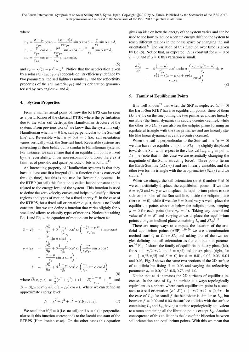
Fig. 5 shows the spectrum of the equilibrium points of the L1

family (top) andL2 family (bottom) that lie on the ecliptic plane(δ = π/2) for β = 0.03. The L1 family has equilibrium pointsof class T1 and T2 whose spectra appears on the left and rightplots respectively. The equilibrium points on the L2 family areall of class T1 where |νi| < 0.001. The right hand side of thebottom plot shows a zoom close to the imaginary axis.

The location of the L1 and L2 AEP is interesting for obser-vational mission applications like SunJammer or the Polar Sit-ter.18 Most of these mission require to remain close to an AEPof class T1 (unstable point) needing an active control law toremain close to them. On the next section we will describethe non-linear dynamics around AEP of class T1 with νi = 0

(Hamiltonian and Reversible case). As we have seen, changingthe reflectivity properties of the sail is equivalent to changingthe sail lightness number and its orientation. For simplicity thecomputations are done for ρr = 1, but similar results are ex-pected for ρ ≈ 1.


-2.5

-2

-1.5

-1

-0.5

0

0.5

1

1.5

2

2.5

-3 -2 -1 0 1 2 3

IM

RE

Spectrum for SL1 AEP (ρ = 0, δ = π = -90o)

λ1,2ν2 – iω2ν3 – iω3

-1.5

-1

-0.5

0

0.5

1

1.5

-1.5 -1 -0.5 0 0.5 1 1.5

IM

RE


ν1 – iω1ν2 – iω2ν3 – iω3

-3

-2

-1

0

1

2

3

-4 -3 -2 -1 0 1 2 3 4

IM

RE


λ1,2ν1 – iω1ν2 – iω2

-3

-2

-1

0

1

2

3

-0.0015 -0.001 -0.0005 0 0.0005 0.001 0.0015

IM

RE


λ1,2ν1 – iω1ν2 – iω2

Fig. 5: Spectrum for equilibria in the L1 (top) and L2 (bottom) familieson the ecliptic plane (δ = π/2) for β = 0.03.

6. Non-linear dynamics around AEP

In this section we want to describe the non-linear dynam-ics around the AEP and how the different sail parameters(β, ρ, α, δ) affects the dynamics. As we have just mentionedwe will focus on the dynamics for class T1 AEP on the L1

and L2, on the Hamiltonian case (α = 0) and Reversible case(α 6= 0, δ = 0). In both cases the linear dynamics is al-ways centre×centre×saddle and we can ensure, that under non-resonant conditions, there exists periodic and quasi-periodic or-bits around the AEP.15, 22 The non-Reversible case (δ 6= 0) iswork in progress.

To describe the non-linear dynamics we compute families ofperiodic orbits for different (fixed) sail parameters. We knowthat each centres gives rise to one family of periodic orbits thatemanate from the AEP. We use a classical continuation schemeto compute these orbits and their main bifurcations. Moreover,the coupling between the two centre frequencies generate fam-ilies of quasi-periodic orbits, also known as Lissajous orbits.There are different ways to compute these orbits (Lindstedt-Poincaré, invariant tori computation or the reduction to the cen-tre manifold). We use the reduction to the centre manifold asit is a fast way to capture the bounded motion close to an AEP.The idea is to decouple the centre from the saddle componentson the equations of motion up to high order and use the flow re-duced on the centre components to produce Poincaré plots.7, 14

The main disadvantage of this procedure is that it is a local, andit will capture the dynamics for energy levels close to the AEP.

6.1. Summary on the dynamics around L1 and L2

We start by describing the unperturbed RTBP, discarding thesolar sail effect (β = 0). The dynamics around L1,2 has beenwell studied in the past,10, 11, 25 here we present the main invari-ant objects which will serve as reference to see how the solar

sail affects the non-linear dynamics around the AEP.The linear dynamics around L1,2 is centre×centre×saddle,

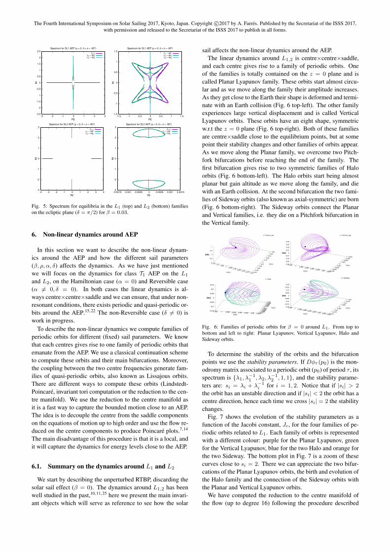
and each centre gives rise to a family of periodic orbits. Oneof the families is totally contained on the z = 0 plane and iscalled Planar Lyapunov family. These orbits start almost circu-lar and as we move along the family their amplitude increases.As they get close to the Earth their shape is deformed and termi-nate with an Earth collision (Fig. 6 top-left). The other familyexperiences large vertical displacement and is called VerticalLyapunov orbits. These orbits have an eight shape, symmetricw.r.t the z = 0 plane (Fig. 6 top-right). Both of these familiesare centre×saddle close to the equilibrium points, but at somepoint their stability changes and other families of orbits appear.As we move along the Planar family, we overcome two Pitch-fork bifurcations before reaching the end of the family. Thefirst bifurcation gives rise to two symmetric families of Haloorbits (Fig. 6 bottom-left). The Halo orbits start being almostplanar but gain altitude as we move along the family, and diewith an Earth collision. At the second bifurcation the two fami-lies of Sideway orbits (also known as axial-symmetric) are born(Fig. 6 bottom-right). The Sideway orbits connect the Planarand Vertical families, i.e. they die on a Pitchfork bifurcation inthe Vertical family.

-1.015-1.01

-1.005-1

-0.995-0.99

-0.985-0.98

-0.975-0.97

-0.05

-0.04

-0.03

-0.02

-0.01

0

0.01

0.02

0.03

0.04

0.05

-1

-0.5

0

0.5

1

Z(AU)

L1 Planar Lyap

X(AU)

Y(AU)

Z(AU)

-1.002-1

-0.998-0.996

-0.994-0.992

-0.99-0.988-0.004

-0.003-0.002

-0.001 0

0.001 0.002

0.003 0.004

-0.04

-0.03

-0.02

-0.01

0

0.01

0.02

0.03

0.04

Z(AU)

L1 Vertical Lyap

X(AU)

Y(AU)

Z(AU)

-1.002 -1 -0.998 -0.996 -0.994 -0.992 -0.99 -0.988-0.01-0.008-0.006-0.004-0.002 0 0.002 0.004 0.006 0.008 0.01

-0.015

-0.01

-0.005

0

0.005

0.01

0.015

Z(AU)

L1 Halo

X(AU)

Y(AU)

Z(AU)

-1.002-1

-0.998-0.996

-0.994-0.992

-0.99-0.988

-0.986-0.02-0.015

-0.01-0.005

0 0.005

0.01 0.015

0.02

-0.02

-0.015

-0.01

-0.005

0

0.005

0.01

0.015

0.02

Z(AU)

L1 SideWay

X(AU)

Y(AU)

Z(AU)

Fig. 6: Families of periodic orbits for β = 0 around L1. From top tobottom and left to right: Planar Lyapunov, Vertical Lyapunov, Halo andSideway orbits.

To determine the stability of the orbits and the bifurcationpoints we use the stability parameters. If Dφτ (p0) is the mon-odromy matrix associated to a periodic orbit (p0) of period τ , itsspectrum is λ1, λ−11 , λ2, λ

−12 , 1, 1, and the stability parame-

ters are: si = λi + λ−1i for i = 1, 2. Notice that if |si| > 2

the orbit has an unstable direction and if |si| < 2 the orbit has acentre direction, hence each time we cross |si| = 2 the stabilitychanges.

Fig. 7 shows the evolution of the stability parameters as afunction of the Jacobi constant, Jc, for the four families of pe-riodic orbits related to L1. Each family of orbits is representedwith a different colour: purple for the Planar Lyapunov, greenfor the Vertical Lyapunov, blue for the two Halo and orange forthe two Sideway. The bottom plot in Fig. 7 is a zoom of thesecurves close to si = 2. There we can appreciate the two bifur-cations of the Planar Lyapunov orbits, the birth and evolution ofthe Halo family and the connection of the Sideway orbits withthe Planar and Vertical Lyapunov orbits.

We have computed the reduction to the centre manifold ofthe flow (up to degree 16) following the procedure described


-4

-2

0

2

4

6

8

10

12

14

-3.001 -3.0008 -3.0006 -3.0004 -3.0002 -3 -2.9998 -2.9996

Sta

bili

ty P

ata

mete

r

Jc

L1 Family of OP

PLyapVLyapHalo

SideWay

1.6

1.8

2

2.2

2.4

-3.001 -3.0008 -3.0006 -3.0004 -3.0002 -3 -2.9998 -2.9996

Sta

bili

ty P

ata

mete

r

Jc

L1 Family of OP

PLyapVLyapHalo

SideWay

Fig. 7: Variation of the stability parameter si for the families of orbitsrelated to L1.

in Farres et al.7 We denote by x1, x2 to the coordinates on thecentre manifold related to the horizontal oscillations and x3, x4to the coordinates related to the vertical oscillation. In orderto visualise the dynamics on these 4D manifold we select thePoincaré section x3 = 0, which is transversal to the verticaloscillations. Then we select an energy level Jc = J0, take amesh of points (x1, x2) and numerically compute the (unique)value x4 such that Jc(x1, x2, 0, x4) = J0 (if such value doesnot exist, it means that there is no orbit with (x1, x2) and thisenergy level crossing x3 = 0). Then we plot the successiveintersections of these trajectories with the Poincaré section. Wenote that slicing at x3 = 0 is equivalent to taking a z = 0

section.Fig. 8 shows this Poincaré section for Jc = −3.000848 (left)

and Jc = −3.000808 (right). The first energy is before the Haloorbits appear and the second after. The fixed point in the middlecorresponds to the Vertical Lyapunov orbit and the boundary isthe Planar Lyapunov orbit. The periodic orbits that orbit aroundthe fixed point are the Lissajous orbits. The two other fixedpoints that appear for Jc = −3.000808 are the two Halo orbits.In order to see the Sideway orbits we need to consider Jc ∈[−3.00025,−3.00010], but the reduction to the centre manifoldis no-longer a good representation for such large energy levels.One should have to compute explicitly the family of invarianttori as it is done by Gomez et al.12 and Farres et al.9

-1.5

-1

-0.5

0

0.5

1

1.5

-1.5 -1 -0.5 0 0.5 1 1.5

x2

x1

CM at L1 for β = 0.00 and Jc = -3.000848

-1.5

-1

-0.5

0

0.5

1

1.5

-1.5 -1 -0.5 0 0.5 1 1.5

x2

x1

CM at L1 for β = 0.00 and Jc = -3.000808

Fig. 8: Centre manifold around L1 for Jc = −3.000848 (left) and Jc =−3.000808 (right).

The plots presented here correspond to the families of peri-odic and quasi-periodic orbits related to L1 but the qualitativebehaviour around L2 is the. Note that this behaviour is for the

Earth-Sun problem where µ is small, in the case of other Planet-Earth RTBP the behaviour around L1 and L2 might not thissymmetric.12, 25 In the following sections the effect of the solarsail on the phase space dynamics is described. Recall that as βincreases both equilibria are displaced towards the Sun, i.e. L1

moves away from the Earth and L2 moves closer to it. Hence,the effect of the SRP on each family will be different.

6.2. Effect on the dynamics around L1 for α = 0

Let us start by setting the sail perpendicular to the Sun-sailline (α = 0), i.e. the Hamiltonian case. We have computed thefamilies of periodic orbits for different β following the sameprocedure as in the non perturbed case (continuation method forperiodic orbits starting at SL1). Keeping track of the variationof the stability parameters and possible bifurcations.

In Fig. 9 shows the variation of the stability parameters as afunction of Jc for β = 0.01, 0.03 and 0.05, and Fig. 10 shows azoom of the previous plot close to si = 2 to better appreciate thedifferent bifurcations. Notice that for these values of β the Pla-nar and Vertical Lyapunov orbits behave in a very similar way,and experience the same bifurcations, which appear for differ-ent energy levels. For instance the bifurcation that gives riseto the Sideway orbits comes close to SL1 as β increases.2 Thebig qualitative change is on the behaviour of the terminationof the Halo family. This was first observed by McInnes,17 andstudied in more detail by Verrier.26 Fig. 11 plots the Poincarésection y = 0, y > 0 of the two orbits in the Halo family forβ = 0, 0.01, 0.03 and 0.05. Notice that for β small the Halo or-bits terminate with an Earth collision, while as β increases theyreach a planar orbit surrounding the Earth.

-4

-2

0

2

4

6

8

10

12

14

-2.9806 -2.9804 -2.9802 -2.98 -2.9798 -2.9796 -2.9794

Sta

bili

ty P

ata

mete

r

Jc

L1 Family of OP β = 0.01

PLyapVLyapHalo

SideWay

-4

-2

0

2

4

6

8

10

12

14

-2.9402 -2.94 -2.9398 -2.9396 -2.9394 -2.9392 -2.939 -2.9388

Sta

bili

ty P

ata

mete

r

Jc


PLyapVLyapHalo

SideWay

-4

-2

0

2

4

6

8

10

12

14

-2.8994 -2.8992 -2.899 -2.8988 -2.8986 -2.8984 -2.8982

Sta

bili

ty P

ata

mete

r

Jc


PLyapVLyapHalo

SideWay

Fig. 9: Variation of the stability parameter si for the families of orbitsrelated to L1. For β = 0.01 (top), β = 0.03 (middle) and β = 0.05(bottom).


1.6

1.8

2

2.2

2.4

-2.9806 -2.9804 -2.9802 -2.98 -2.9798 -2.9796 -2.9794

Sta

bili

ty P

ata

mete

r

Jc


PLyapVLyapHalo

SideWay

1.6

1.8

2

2.2

2.4

-2.9402 -2.94 -2.9398 -2.9396 -2.9394 -2.9392 -2.939 -2.9388

Sta

bili

ty P

ata

mete

r

Jc


PLyapVLyapHalo

SideWay

1.6

1.8

2

2.2

2.4

-2.8994 -2.8992 -2.899 -2.8988 -2.8986 -2.8984 -2.8982

Sta

bili

ty P

ata

mete

r

Jc


PLyapVLyapHalo

SideWay

Fig. 10: Zoom around si = 2 of Fig. 9. For β = 0.01 (top), β = 0.03(middle) and β = 0.05 (bottom).

-0.02

-0.015

-0.01

-0.005

0

0.005

0.01

0.015

0.02

-1 -0.99 -0.98 -0.97 -0.96 -0.95 -0.94

EarthZ (

AU

)

X (AU)

β = 0.00β = 0.01β = 0.03β = 0.05

Fig. 11: Poincaré section Y = 0 for the two periodic orbits on the Halofamily for β = 0, 0.01, 0.03 and 0.05.

6.3. Effect on the dynamics around L2 for α = 0

Let us now focus on the L2 for α = 0, where we have alsocomputed the families of periodic orbits using a continuationmethod starting at SL2. There is also a planar and a verticaloscillation related to Planar and Vertical Lyapunov orbits andmany bifurcations along the families.

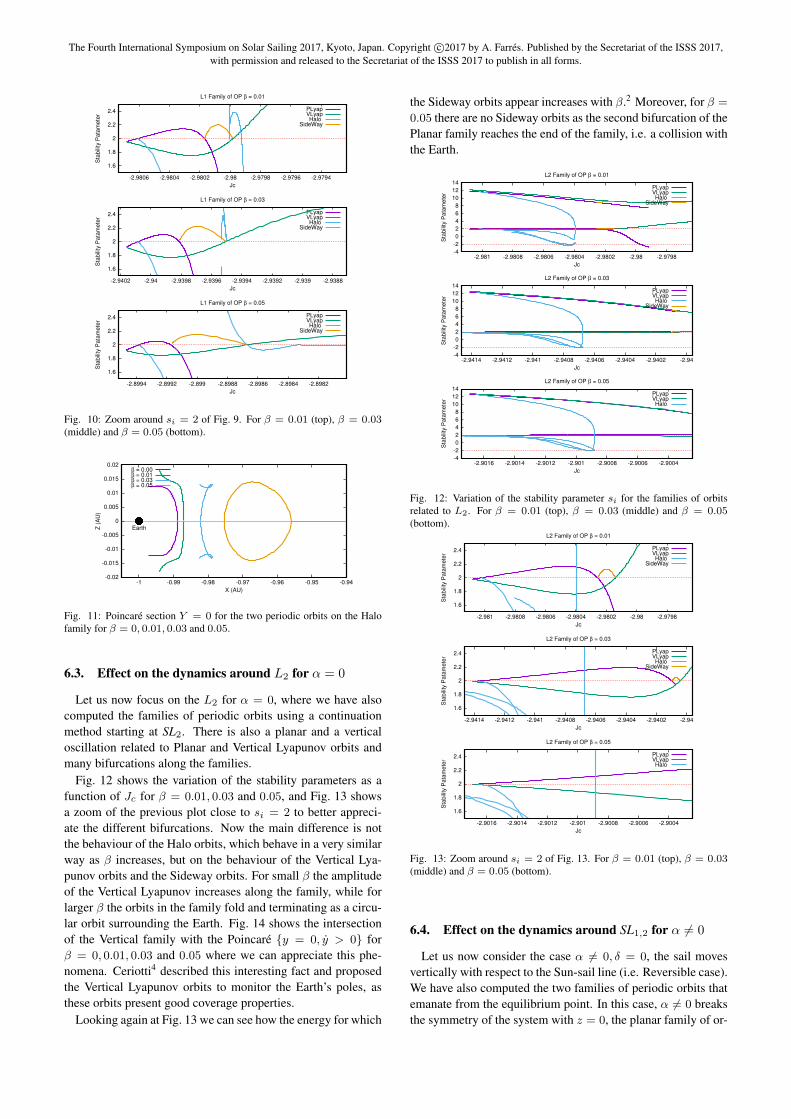
Fig. 12 shows the variation of the stability parameters as afunction of Jc for β = 0.01, 0.03 and 0.05, and Fig. 13 showsa zoom of the previous plot close to si = 2 to better appreci-ate the different bifurcations. Now the main difference is notthe behaviour of the Halo orbits, which behave in a very similarway as β increases, but on the behaviour of the Vertical Lya-punov orbits and the Sideway orbits. For small β the amplitudeof the Vertical Lyapunov increases along the family, while forlarger β the orbits in the family fold and terminating as a circu-lar orbit surrounding the Earth. Fig. 14 shows the intersectionof the Vertical family with the Poincaré y = 0, y > 0 forβ = 0, 0.01, 0.03 and 0.05 where we can appreciate this phe-nomena. Ceriotti4 described this interesting fact and proposedthe Vertical Lyapunov orbits to monitor the Earth’s poles, asthese orbits present good coverage properties.

Looking again at Fig. 13 we can see how the energy for which

the Sideway orbits appear increases with β.2 Moreover, for β =

0.05 there are no Sideway orbits as the second bifurcation of thePlanar family reaches the end of the family, i.e. a collision withthe Earth.

-4

-2

0

2

4

6

8

10

12

14

-2.981 -2.9808 -2.9806 -2.9804 -2.9802 -2.98 -2.9798

Sta

bili

ty P

ata

mete

r

Jc


PLyapVLyapHalo

SideWay

-4

-2

0

2

4

6

8

10

12

14

-2.9414 -2.9412 -2.941 -2.9408 -2.9406 -2.9404 -2.9402 -2.94

Sta

bili

ty P

ata

mete

r

Jc


PLyapVLyapHalo

SideWay

-4

-2

0

2

4

6

8

10

12

14

-2.9016 -2.9014 -2.9012 -2.901 -2.9008 -2.9006 -2.9004

Sta

bili

ty P

ata

mete

r

Jc


PLyapVLyapHalo

Fig. 12: Variation of the stability parameter si for the families of orbitsrelated to L2. For β = 0.01 (top), β = 0.03 (middle) and β = 0.05(bottom).

1.6

1.8

2

2.2

2.4

-2.981 -2.9808 -2.9806 -2.9804 -2.9802 -2.98 -2.9798

Sta

bili

ty P

ata

mete

r

Jc


PLyapVLyapHalo

SideWay

1.6

1.8

2

2.2

2.4

-2.9414 -2.9412 -2.941 -2.9408 -2.9406 -2.9404 -2.9402 -2.94

Sta

bili

ty P

ata

mete

r

Jc


PLyapVLyapHalo

SideWay

1.6

1.8

2

2.2

2.4

-2.9016 -2.9014 -2.9012 -2.901 -2.9008 -2.9006 -2.9004

Sta

bili

ty P

ata

mete

r

Jc


PLyapVLyapHalo

Fig. 13: Zoom around si = 2 of Fig. 13. For β = 0.01 (top), β = 0.03(middle) and β = 0.05 (bottom).

6.4. Effect on the dynamics around SL1,2 for α 6= 0

Let us now consider the case α 6= 0, δ = 0, the sail movesvertically with respect to the Sun-sail line (i.e. Reversible case).We have also computed the two families of periodic orbits thatemanate from the equilibrium point. In this case, α 6= 0 breaksthe symmetry of the system with z = 0, the planar family of or-


-0.005

0

0.005

0.01

0.015

0.02

0.025

-1.01 -1.005 -1 -0.995 -0.99 -0.985

Earth

Z (

AU

)

X (AU)

β = 0.00β = 0.01β = 0.03β = 0.05

Fig. 14: Poincaré section Y = 0, Y > 0 for the periodic orbits on theVertical Lyapunov family for β = 0, 0.01, 0.03 and 0.05.

bits are no longer contained on the plane and gain altitude as weincrease Jc and their shape resembles a Halo type orbits. More-over, there is no longer a Pitchfork bifurcation, actually this onehas been replaced by a Saddle-Node bifurcation. Fig. 15 showsthe Poincaré section of the Planar and Halo type orbits fromβ = 0.03 and α = 0 (left), α = 0.01 rad (right). There wecan see the effect of the symmetry breaking and how the Planarand Halo families are related to each other in a different wayfor α 6= 0. For further details see Farres.8

-0.015

-0.01

-0.005

0

0.005

0.01

0.015

-0.985 -0.983 -0.981 -0.979 -0.977

Z (

AU

)

X (AU)

L1 Family of OP β = 0.03, α = 0.000, δ = 0.00

cxssxscxc

-0.015

-0.01

-0.005

0

0.005

0.01

0.015

-0.986 -0.984 -0.982 -0.98 -0.978

Z (

AU

)

X (AU)

L1 Family of OP β = 0.03, α = 0.010, δ = 0.00

cxssxscxc

Fig. 15: Poincaré section y = 0, y > 0 for the periodic orbits on thePlanar Lyapunov and Halo orbits at SL1for β = 0.03, δ = 0 and α = 0 rad(left) and α = 0.01 rad (right).

Fig. 16 shows the variation of the stability parameters as afunction of the energy for β = 0.03 and α = 0.01 rad at SL1

(similar behaviour is found at SL2. The bottom plot shows azoom close to si = 2 to appreciate better the bifurcations. Therewe see the symmetry breaking on the Halo family of orbits. Wealso see that the second bifurcation on the Planar family, whichgives rise to the Sideway orbits, still exists. Notice that thissecond bifurcation has not been broken by α 6= 0 due to thenature of the orbits.

We have also computed the reduction to the centre manifoldaround different AEP for β = 0.03, and used it to describe thebounded motion around the AEP. Fig. 17 shows Poincaré sec-tions on the centre manifold around the AEP for α = 0 (top)and α = 0.01 (bottom). Notice that the behaviour for α = 0 issimilar to the one for β = 0 (Fig. 8), where we can see that forsmall Jc we only have a Vertical Lyapunov orbit as a fixed pointclose to the origin, Lissajous orbits surrounding the point andthe boundary would correspond to the Planar Lyapunov orbit.For a larger Jc the two Halo orbits appear. The main differenceis values of Jc for which the different bifurcations take place.If we look at α = 0.01 (bottom), we see that for small Jc thereis an extra fixed point on the right hand side of the plot. Thisorbit corresponds to the Planar Lyapunov orbit that is no longer

-4

-2

0

2

4

6

8

10

12

14

-2.9402 -2.94 -2.9398 -2.9396 -2.9394 -2.9392 -2.939 -2.9388

Sta

bili

ty P

ata

mete

r

Jc

L1 Family of OP β = 0.03, α = 0.010, δ = 0.00

PLyapVLyapHalo

SideWay

1.6

1.8

2

2.2

2.4

-2.9402 -2.94 -2.9398 -2.9396 -2.9394 -2.9392 -2.939 -2.9388

Sta

bili

ty P

ata

mete

r

Jc

L1 Family of OP β = 0.03, α = 0.010, δ = 0.00

PLyapVLyapHalo

SideWay

Fig. 16: Variation of the stability parameter si for the families of orbitsrelated to SL1. For β = 0.03, δ = 0 and α = 0.01 rad. Bottom plot is azoom close to si = 2.

contained on x3 = 0, and is no longer the boundary of the mo-tion. If we increase Jc we see the two Halo type orbits as fixedpoints, we can also appreciate the asymmetry of the section dueto the symmetry breaking.

-2

-1.5

-1

-0.5

0

0.5

1

1.5

2

-2 -1.5 -1 -0.5 0 0.5 1 1.5 2

x2

x1

CM at L1 for β = 0.00 and Jc = -2.940096

-2

-1.5

-1

-0.5

0

0.5

1

1.5

2

-2 -1.5 -1 -0.5 0 0.5 1 1.5 2

x2

x1

CM at L1 for β = 0.00 and Jc = -2.940009

-2

-1.5

-1

-0.5

0

0.5

1

1.5

2

-2 -1.5 -1 -0.5 0 0.5 1 1.5 2

x2

x1

CM at L1 for β = 0.00 and Jc = -2.940096

-2

-1.5

-1

-0.5

0

0.5

1

1.5

2

-2 -1.5 -1 -0.5 0 0.5 1 1.5 2

x2

x1

CM at L1 for β = 0.00 and Jc = -2.940009

Fig. 17: Centre manifold around SL1 for β = 0.03 and Jc = −2.940096(left) and Jc = −2.940009 (right). Top: α = 0 rad, Bottom: α =0.01 rad

7. Conclusions

In this paper some relevant aspects of the dynamics of a so-lar sail in the Earth-Sun RTBP have been described, and therichness on the dynamics when varying the sail parameters(β, ρ, α, δ) has been highlighted. Moreover, the combinationof computation of families of periodic orbits and the reduc-tion to the centre manifold gives an accurate description of thebounded motion close to the AEP.

It is still work in progress the description of the dynamicswhen δ 6= 0. Here the system is no longer Reversible and we


cannot ensure the existence of periodic and quasi-periodic mo-tion around an AEP. Nevertheless, as we have seen in section 5.the instability given by the centre components is very mild inmany cases. Hence, there might be almost periodic and almostquasi-periodic orbits of interesting for mission applications.

The final goal of this project is to catalogue the different typeof periodic orbits as a function of the sail parameters. Suchcatalogue would enable the astrodynamics community enhanceopportunities for solar sail and other low-thrust propulsion sys-tems. Moreover, a good understanding on the variation of thedynamics with respect to the sail parameters is useful when de-riving station keeping manoeuvres and other control laws.

Acknowledgements

This research has been supported by the Spanish grantMTM2015-67724-P (funded by MINECO/FEDER, UE) andthe Catalan grant 2014 SGR 1145.

References

[1] G. Aliasi, G. Mengali, and A. Quarta. Artificial equilibrium pointsfor a generalized sail in the circular restricted three-body problem.Celestial Mechanics and Dynamical Astronomy, 110:343–368, 2011.

[2] M. Ceccaroni, A. Celletti, and G. Pucacco. Birth of periodic and ar-tificial halo orbits in the restricted three-body problem. InternationalJournal of Non-Linear Mechanics, 81:65 – 74, 2016.

[3] M. Ceriotti and C. McInnes. A near term pole-sitter using hybridsolar sail propulsion. In R. Kezerashvili, editor, Proc. of the SecondInternational Symposium on Solar Sailing, pages 163–169, July 2010.

[4] M. Ceriotti and C. McInnes. Natural and sail-displaced doubly-symmetric lagrange point orbits for polar coverage. Celestial Me-chanics and Dynamical Astronomy, 114(1-2):151–180, 2012.

[5] B. Dachwald, W. Seboldt, M. Macdonald, G. Mengali, A. Quarta,C. McInnes, L. Rios-Reyes, D. Scheeres, B. Wie, M. Görlich, et al.Potential Solar Sail Degradation Effects on Trajectory and AttitudeControl. In AAS/AIAA Astrodynamics Specialists Conference, 2005.

[6] A. Farrés. Transfer orbits to l4 with a solar sail in the earth-sun sys-tem. Acta Astronautica, 2016. (submitted).

[7] A. Farrés and À. Jorba. On the high order approximation of the centremanifold for ODEs. Discrete and Continuous Dynamical Systems -Series B (DCDS-B), 14:977–1000, October 2010.

[8] A. Farrés and À. Jorba. Periodic and quasi-periodic motions of asolar sail around the family SL1 on the Sun-Earth system. CelestialMechanics and Dynamical Astronomy, 107:233–253, 2010.

[9] A. Farrés, À. Jorba, and J. Mondelo. Orbital dynamics for a non-perfectly reflecting solar sail close to an asteroid. In Proceedings ofthe 2nd IAA Conference on Dynamics and Control of Space Systems,Rome, Italy, 2014.

[10] G. Gómez, À. Jorba, J. Masdemont, and C. Simó. Dynamics andMission Design Near Libration Points - Volume III: Advanced Meth-ods for Collinear Points., volume 4 of World Scientific MonographSeries in Mathematics. World Scientific, 2001.

[11] G. Gómez, J. Llibre, R. Martínez, and C. Simó. Dynamics and Mis-sion Design Near Libration Points - Volume I: Fundamentals: TheCase of Collinear Libration Points, volume 2 of World ScientificMonograph Series in Mathematics. World Scientific, 2001.

[12] G. Gómez and J. Mondelo. The dynamics around the collinear equi-librium points of the RTBP. Physica D, 157(4):283–321, 2001.

[13] J. Heiligers, B. Diedrich, B. Derbes, and C. McInnes. Sunjam-mer: Preliminary end-to-end mission design. In Proceedings of theAIAA/AAS Astrodynamics Specialist Conference, 2014.

[14] À. Jorba and J. Masdemont. Dynamics in the centre manifold of thecollinear points of the Restricted Three Body Problem. Physica D,132:189–213, 1999.

[15] J. Lamb and J. Roberts. Time-reversal symmetry in dynamical sys-tems: a survey. Phys. D, 112:1–39, 1998.

[16] J. Masdemont and J. Mondelo. Notes for the numerical and analyti-cal techniques. Advanced Topics in Astrodynamics, Summer Course,July 2004.

[17] A. McInnes. Strategies for solar sail mission design in the circularrestricted three-body problem. Master’s thesis, Purdue University,August 2000.

[18] C. McInnes. Solar Sailing: Technology, Dynamics and Mission Ap-plications. Springer-Praxis, 1999.

[19] C. McInnes, A. McDonald, J. Simmons, and E. MacDonald. Solarsail parking in restricted three-body system. Journal of Guidance,Control and Dynamics, 17(2):399–406, 1994.

[20] C. R. McInnes. Artificial Lagrange Points for a Partially Reflect-ing Flat Solar Sail. Journal of Guidance, Control, and Dynamics,22(1):185–187, jan 1999.

[21] C. R. McInnes, V. Bothmer, B. Dachwald, U. R. M. E. Geppert,J. Heiligers, A. Hilgers, L. Johnson, M. Macdonald, R. Reinhard,W. Seboldt, and P. Spietz. Gossamer Roadmap Technology ReferenceStudy for a Sub-L1 Space Weather Mission, pages 227–242. SpringerBerlin Heidelberg, Berlin, Heidelberg, 2014.

[22] K. Meyer and G. Hall. Introduction to Hamiltonian Dynamical Sys-tems and the N-Body Problem. Springer, New York, 1992.

[23] L. Rios-Reyes and D. Scheeres. Generalized model for solar sails.Journal of Spacecraft and Rockets, 42(1):182–184, 2005.

[24] C. Simó. Effective computations in celestial mechanics and astro-dynamics. In V. Rumyantsev and A. Karapetyan, editors, ModernMethods of Analytical Mechanics and their Applications, volume 387of CISM Courses and Lectures. Springer Verlag, 1998.

[25] V. Szebehely. Theory of orbits. The restricted problem of three bodies.Academic Press, 1967.

[26] P. Verrier, T. Waters, and J. Sieber. Evolution of the l1 halo family inthe radial solar sail circular restricted three-body problem. CelestialMechanics and Dynamical Astronomy, 120(4):373–400, 2014.

Catalogue on the Dynamics of a Solar Sail around L1 and L2

Documents

Transcript of Catalogue on the Dynamics of a Solar Sail around L1 and L2