AN ABSTRACT OF THE THESIS OF Katelyn M. Cassidy for the degree of Master of Science in Fisheries Science presented on December 5, 2008. Title: Use of Extractable Lipofuscin as an Age Biomarker to Determine Age Structure of Ghost Shrimp (Neotrypaea californiensis) Populations in West Coast Estuaries Abstract approved: ___________________________________________________________ Brett R. Dumbauld Christopher J. Langdon Determining age in crustaceans is inherently imprecise because they molt

periodically and do not retain hard structures throughout their lifespan. Morphological

measurements, such as carapace length, are often used to estimate age because

methods for direct ageing do not exist. However, variability in individual growth rate

and molt frequency can result in a wide distribution of sizes in a single age class,

making length a poor predictor of true age. Research examining the autofluorescent

age pigment, lipofuscin, suggests that concentration of the pigment in neural tissues is

directly related to actual age. Analysis of lipofuscin concentration has already proven

to be a more effective method for determining true age in several species of

crustaceans than traditional, length-based methods. The ghost shrimp, Neotrypaea

californiensis, negatively impacts oyster aquaculture in Pacific Northwest estuaries.

Current efforts to develop an integrated pest management plan for this species would

benefit from better information on the age and growth of these animals. This study

3 assessed the potential of using extractable lipofuscin as a method for determining age

in N. californiensis. A growth study was conducted to validate the lipofuscin aging

technique and develop a practical method of age determination for this species.

Lipofuscin-based aging was used to determine age structures for three populations of

N. californiensis and these were compared to age structures determined using

traditional length-based methods. Age structures determined with analysis of

lipofuscin concentration revealed several more age classes than assessments based on

carapace length measurements in all sampled populations. Comparison of mean size-

at-age among populations in Oregon and Washington estuaries showed growth rate

varied spatially. Site-specific environmental factors like food availability, population

density and tidal elevation may affect individual and population growth patterns. In

this study, analysis of extractable lipofuscin proved to be a more accurate method of

age determination than body-length measurements. The data presented here show that

biochemical-based aging can now be widely used to assess age in N. californiensis,

facilitating more in-depth investigations of basic biological and ecological processes

for this species.

©Copyright by Katelyn M. Cassidy

December 5, 2008

All Rights Reserved

Use of Extractable Lipofuscin as an Age Biomarker to Determine Age Structure of Ghost Shrimp (Neotrypaea californiensis) Populations in West Coast Estuaries

by Katelyn M. Cassidy

A THESIS

Submitted to

Oregon State University

in partial fulfillment of the requirements for the

degree of

Master of Science

Presented December 5, 2008 Commencement June 2009

Master of Science thesis of Katelyn M. Cassidy presented on December 5, 2008. APPROVED: ____________________________________________________________________

Co-Major Professor, representing Fisheries Science

____________________________________________________________________

Co-Major Professor, representing Fisheries Science

____________________________________________________________________

Head of the Department of Fisheries and Wildlife

____________________________________________________________________

Dean of the Graduate School

I understand that my thesis will become part of the permanent collection of Oregon State University libraries. My signature below authorizes release of my thesis to any reader upon request. ____________________________________________________________________

Katelyn M. Cassidy, Author

ACKNOWLEDGEMENTS

I would like to express my sincere appreciation to my major advisor, Dr. Brett

Dumbauld. Thank you for providing me with all the resources I needed to complete

this project. Your undying support, encouragement, patience and guidance has been

my driving force over the last three years. Thank you for being a true inspiration and

teaching me to love all things that live in the mud. Thanks to my other committee

members: Chris Langdon for keeping me on track, and Tony D’Andrea for always

reminding me to look at the big picture. Thanks to Lee McCoy, for not only being my

technical and mechanical support, but also a friend. Thanks Lee for taking the

monotony out of fieldwork and always making me laugh. I would like to recognize

Cara Fritz for helping with processing samples and being a second set of hands in the

hatchery; Roy Hildenbrand for driving the boat and helping in the field; and all others

that I have dragged out on the tideflat to assist with sampling. Digging holes in the

mud is a tough job. My sincere appreciation to Dr. Jim Dombrowki of the USDA-ARS

Forage Seed and Cereal Unit for the use of your autosampler over last three years; and

the employees of the USEPA Coastal Ecology Branch in Newport, OR, especially Bob

Randall for always making sure that I had everything I need and Jim Power for the use

of the spectrophotometer. Also, thanks to Se-Jong Ju, who answered my questions and

provided me guidance when I was struggling along in the early stages of this project.;

Pat Clinton of EPA and Keven Bennett of the Olympic Natural Resources Center for

providing tidal elevation data for my study sites. Thanks to my mother and father, who

always believed that I could do anything and for their unconditional love and support.

8 Thanks to Marisa Litz, for joining me in charging Oregon waves over the last three

years and Tristan Britt for reminding me to relax and have fun. And finally, thanks to

Keith Bosley for being my number one fan and teaching me that you can have

everything you want in life. None of this work would have been possible without the

help of all the people mentioned here. This work was supported by the USDA–ARS

and the 2007 and 2008 Mamie Markham Awards.

CONTRIBUTION OF AUTHORS

Dr. Brett R. Dumbauld provided recruitment and long-term monitoring data for

chapters 2 and 3. He also reviewed and provided comments on Chapters 1, 2 and 3.

Drs. Christopher J. Langdon and Anthony D’Andrea reviewed and provided

comments on chapters 1, 2, and 3.

TABLE OF CONTENTS Page Chapter 1: General introduction and overview …........................................ 1 General biology and ecology of the ghost shrimp, Neotrypaea californiensis.................................................................................... 1 Pitfalls in assessing age with length-based methods ........................ 5 Overview of lipofuscin and its use as an age biomarker .................. 6 Ghost shrimp as pests for commercial oyster culture ...................... 11 Significance of research ................................................................... 14

LITERATURE CITED ..................................................................... 16 Chapter 2: Verification of lipofuscin-based age determination for the ghost shrimp, Neotrypaea californiensis .......................................... 26 ABSTRACT ..................................................................................... 26 INTRODUCTION ............................................................................ 28 MATERIALS AND METHODS...................................................... 30 RESULTS ........................................................................................ 37 DISCUSSION .................................................................................. 40 LITERATURE CITED..................................................................... 49 Chapter 3: Assessment of population age structure for the ghost

shrimp, Neotrypaea californiensis, in West Coast estuaries using extractable lipofuscin as an age biomarker ...................... 68

ABSTRACT ..................................................................................... 68 INTRODUCTION ............................................................................ 70 MATERIALS AND METHODS...................................................... 72 RESULTS ....................................................................................... 79

11 TABLE OF CONTENTS (Continued)

Page DISCUSSION.................................................................................. 83 LITERATURE CITED..................................................................... 93 Chapter 4: Summary and future directions.................................................... 120 LITERATURE CITED..................................................................... 123 Bibliography ................................................................................................. 124 APPENDICES............................................................................................... 137 Appendix A........................................................................................ 138 Appendix B........................................................................................ 140 Appendix C........................................................................................ 143 Appendix D....................................................................................... 145

LIST OF FIGURES

Figure Page 1.1 Long-term ghost shrimp recruitment at the Palix River in Willapa Bay, Wash.…………………………................................... 24 1.2 Ghost shrimp recruitment at both Palix River in Willapa Bay, Wash., and Idaho Flats in Yaquina Bay, Ore......................................... 24 1.3 Comparison of length-frequency histograms from three populations of Neotrypaea californiensis ........................................ 25 2.1 Map of Yaquina Bay, Oregon showing sites for field calibration study.................................................................................................. 54

2.2 Total fluorescence spectrum from a concentrated extract of N. californiensis brain tissue.............................................................. 55 2.3 Excitation spectrum of brain tissue extract along a single emission wavelength ....................................................................................... 56

2.4 Regression results of pooled LF index data from all three study sites in Yaquina Bay showing relationship of LF index to time ….. 57 2.5 Results of Modal Progression Analysis (MPA) of length-

frequency histograms of male and female N. californiensis from Idaho Flats.......................................................................................... 58

2.6 Results of multiple linear regression analysis showing difference in growth rate of a cohort planted across three sites in Yaquina Bay, Ore............................................................................................. 59 2.7 Results of multiple linear regression analysis showing positive

relationship between LF index and time (day) from three sites in Yaquina Bay, Ore.............................................................................. 60

2.8 Average monthly temperature at three study sites in Yaquina Bay, Oregon ..................................................................................... 61 2.9 Temperature fluctuations experienced at all three study sites over two tidal cycles in July 2007............................................................. 62

3.1 Maps of Willapa Bay, Wash. and Yaquina Bay, Ore. showing survey locations within each bay ..................................................... 99

13 LIST OF FIGURES (Continued)

Figure Page 3.2 Length-frequency distributions from each survey site ......................100 3.3 Results of Modal Progression Analysis of length-frequency data collected from male N. californiensis................................................ 101 3.4 Results of Modal Progression Analysis of length-frequency data collected from female N. californiensis............................................ 102 3.5 Results of MPA of LF index data from spring and fall 2007............ 103

3.6 Regression of mean LF index against LF-estimated age for all three sites assessed ............................................................................ 104

3.7 Multiple linear regression of pooled LF index-at-age data from

spring and fall sample periods assuming equal slopes...................... 105

3.8 LF index-frequency histograms from April 2007 with bars representing age classes as determined from MPA of CL- frequency histograms......................................................................... 106

3.9 LF-based age model for N. californiensis populations in Willapa Bay, Wash., and Yaquina Bay, Ore. ....................................107

3.10 Scatterplot showing the relationship of carapace length to LF-estimated age................................................................................ 108

3.11 Recruitment history of N. californiensis in Willapa Bay, Wash., and Yaquina Bay, Ore. ...................................................................... 109

3.12 Change in shrimp density at the three study locations over time...... 110

LIST OF TABLES

Table Page 2.1 Results from Pearson’s correlation between fluorescence

intensities obtained from all five Ex/Em maxima observed in N. californiensis…........................................................................ 63

2.2 Results of regression analysis between LF index and time for two major Ex/Em maxima found in brain tissue of N. californiensis..... 64 2.3 Results of MPA of length-frequency data from April survey

2007................................................................................................... 65 2.4 Results of regression analysis examining effects of time and site on body size (CL (mm)) and LF index (ng LF µg protein-1)............. 66 2.5 Results of One-Way ANOVA testing for difference in average LF concentration from samples processed fresh and those previously frozen ............................................................................. 67

3.1 Palix River age structure as determined by MPA of length- frequency data ................................................................................... 111 3.2 Middle Island Sands age structure as determined by MPA of

length-frequency data….....................................................................112

3.3 Idaho Flats age structure as determined by MPA of length- frequency data.................................................................................... 113 3.4 Palix River age structure as determined by MPA of LF index- frequency data ................................................................................. 114 3.5 Middle Island Sands age structure as determined by MPA of LF index-frequency data ................................................................... 115 3.6 Idaho Flats age structure as determined by MPA of LF index- frequency data ................................................................................... 116 3.7 Table showing increase in average LF concentration for each age class between spring and fall 2007 ................................................... 117

2 LIST OF TABLES (Continued)

Table Page 3.8 Results of multiple linear regression of mean LF index and site against LF-estimated age................................................................... 118 3.9 Results of multiple linear regression of size to LF-estimated age for both sexes................................................................................... 119 3.10 Parameter estimation for the Von Bertalanffy growth function (Eq. 2) modeled by size-at-age for each survey site ......................... 119

LIST OF APPENDIX FIGURES

Figure Page

A1 Molt stage data for N. californiensis in Yaquina Bay, Ore............... 138

A2 Stage duration of N. californiensis larvae cultured at 12 ºC............. 139

B1 Standard curve of quinine sulfate in 0.1N H2SO4 used to quantify LF concentration in brain tissue samples of N. californiensis……... 140 B2 Matrix of correlated fluorescence intensities from 5 Ex/Em maxima observed in N. californiensis.............................................. 141

B3 Comparison of LF concentration from shrimp processed frozen and those frozen two weeks and six months ..................................... 142

D1 Scatterplot and linear regression showing relationship of LF concentration to carapace length in previously frozen N. californiensis with outliers removed................................................. 146

LIST OF APPENDIX TABLES

Table Page

A1 Duration of larval stages of N. californiensis cultured at 12 º C...... 139 C1 Mean body size and LF data from each sample collected for the field growth/calibration experiment .................................................. 143 C2 Average monthly temperature from temperature probes placed 10 cm below the sediment surface at each study site in Yaquina Bay .................................................................................................... 144 D1 Outlying data points from April survey that were removed from the analyses ....................................................................................... 147 D2 Outlying data points from September survey that were removed from the analyses .............................................................................. 148 D3 Results of simple linear regression analyses of LF concentration and protein concentration against carapace length for all three sites surveyed with outliers removed......................................................... 149

Chapter 1: General introduction and overview

Age structure is a key element in population dynamics and ecological

modeling. Obtaining accurate estimates of age in crustaceans has posed a significant

problem for ecologists and managers interested in studying basic biological processes

of this taxonomic group. This study investigates the feasibility and practicality of

using an alternative biochemical approach to determine age in the burrowing

thalassinid shrimp, Neotrypaea californiensis, to replace traditional length-based

methods of age determination which are inherently imprecise. In this study N.

californiensis is used as a model organism because it plays an important ecological

role in West Coast estuaries, but also as a pest to oyster growers operating in the

Pacific Northwest causing significant economic loss. Currently investigation is

underway to gain a better understanding of the ghost shrimp and how it functions in

the environment. Establishing a reliable method for assessing age in N. californiensis

will provide a tool for researchers studying population biology, aid in the development

of effective management strategies and further understanding of age and growth in this

species.

General biology and ecology of the ghost shrimp, Neotrypaea californiensis

Range and distribution

The ghost shrimp, Neotrypaea californiensis Dana 1854 (formerly Callianassa

californiensis; Manning and Felder 1991), is the dominant thalassinid shrimp species

found in estuaries along the Pacific Coast of North America. This species inhabits vast

2 expanses of intertidal mudflats, alters sediment composition and structure, and

influences benthic communities by constructing extensive gallery systems in soft

estuarine sediments (MacGinitie 1929; Posey 1986; Posey 1987). The geographic

range of N. californiensis extends from Alaska to Baja California, Mexico

(MacGinitie, 1934). These animals are easily identified on intertidal mudflats by the

characteristic volcano-shaped mounds that form around their burrow openings. Early

observations of ghost shrimp showed that N. californiensis is generally found in sandy

or muddy sediments at a tidal elevation of zero to +1 foot (MacGinitie, 1934).

However, recent work examining the distribution of ghost shrimp in Willapa Bay

shows shrimp inhabiting a wider tidal range of -4 ft to +4 ft elevation. The greatest

concentration of animals is found between 0 to +2 feet (Dumbauld unpubl.).

Population densities vary spatially and with increasing distance from the

mouth of the estuary. Surveys of ghost shrimp populations along the U.S. West Coast

show N. californiensis densities can range anywhere from 50 to 700 animals m-2

depending on geographic location and distance from the mouth of the Bay (Bird 1982;

Posey, 1986; Swinbanks and Luternaur, 1987; Griffis and Suchanek 1991; Dumbauld

et al. 1996). Studies examining N. californiensis on the Oregon Coast showed

significantly higher densities of shrimp in the lower estuary relative to densities found

at sites in the upper estuary for populations at Sand Lake, Alsea Bay and Yaquina

Bay; however, population density varied among these estuaries for shrimp beds at a

given distance from the mouth of the bay (Bird 1982). Food availability, salinity,

temperature and annual recruitment of new animals to the intertidal are potential

3 mechanisms which likely play a role in determining the density and distribution of

ghost shrimp in West Coast estuaries.

Feeding and Lifestyle

N. californiensis is a motile deposit feeder that feeds primarily on detritus and

microorganisms buried in estuarine sediments (MacGinitie 1934; Powell 1974; Griffis

and Suchanek 1991). This species constructs a system of branching feeding burrows

through the substrate at depths up to 50 cm (Swinbanks and Luternauer 1987). While

adjacent burrows often connect to each other, each burrow only contains a single

shrimp (Swinbanks and Murray 1981). Studies on the burrowing activities of many

thalassinid shrimp have recognized this group as important ecosystem engineers and

bioturbators in benthic estuarine systems. Burrowing activities are important in the

function of the entire estuary, facilitating nutrient remineralization, oxygenation of

sediment and providing habitat for microbial and meiofauna (Berkenbusch & Rowden

2003; Dewitt et al. 2004; Howe et al. 2004 ). Swinbanks and Luternauer (1987)

reported average sediment reworking rates of 18 ± 9 wet ml of sediment shrimp-1day -1

for N. californiensis in the Fraser Delta in British Columbia. These high rates of

sediment reworking modify intertidal substrate and strongly impact benthic

communities associated with burrowing shrimp populations.

Life History and Recruitment

N. californiensis has a complex life-history which involves adult, juvenile and

free-swimming planktonic larval stages. Reproductive females become ovigerous in

early spring (April-May). Developing eggs are carried by the female through the

summer months (June-August), after which newly-hatched larvae are released into the

4 water column (Dumbauld et al. 1996). The planktonic larval stage remains in the water

column for 10-12 weeks (Dumbauld unpub.). During this pelagic stage, the animal

goes through 5 zoeal stages before settling to the benthos as a postlarva (McCrow

1972). Laboratory investigations of ghost shrimp larval development have shown each

larval stage to vary in duration with stages 1, 2, and 3 averaging 11 ± 6 days, stage 4

averaging 20 ± 11.4 days and stage 5 persisting for 17 ± 9.7 days when cultured at 12

ºC (Dumbauld unpub).

Larval dispersal of N. californiensis takes place in the nearshore coastal ocean.

Upwelling conditions and ocean currents during the summer months have been shown

transport larvae of benthic macroinvertebrates 100-200 km from where they were

released in only three months (Botsford et al. 1998). Plankton samples collected off

the Oregon and Washington coasts during summer typically contain advanced stage

larvae, suggesting that larval development largely occurs in the nearshore (D’Andrea,

unpubl; Dumbauld et al. 1996). Records of recruitment in Willapa Bay show strong

inter-annual variability in recruitment strength. Recruitment of 0+ animals ranged

from 144 shrimp m-2 in 1993, 22 shrimp m-2 in 1994, 0 shrimp in 1995 and 1996, and

6 shrimp m-2 in 1997 (Feldman et al. 2000). The largest recruitment events occurred

in the early 1990’s and since that time, recruitment has been extremely low (Figures

1.1, 1.2). It is likely that the magnitude of recruitment in a given year is strongly

influenced by oceanic processes during the time that larvae are in the nearshore coastal

environment. This type of environmental effect has been shown for other decapod

crustaceans with complex life histories, such as Dungeness crab (Shanks and Roegner

2007). Annual recruitment of new animals is an important factor in determining the

5 spatial extent and average age of an adult population. Previous life-history studies on

N. californiensis have examined recruitment, size-at-maturity, growth rate and

mortality for populations in Oregon and Washington estuaries (Bird 1982; Dumbauld

1994; Dumbauld et al. 1996; Feldman et al. 2000), but much remains unknown about

factors influencing the population dynamics of this species. Modeling population

dynamics typically requires accurate estimates of age and this has posed a major

problem for researchers studying crustacean population biology.

Pitfalls in assessing age with length-based methods

Age is a critical parameter for many population dynamics models. Unlike

finfish, which secrete annual bony deposits to otoliths, crustaceans do not retain any

morphological evidence of age or growth throughout their lifespan. All hard structures

are shed with each molt and this lack of bony material has posed a major problem in

identifying chronological age in these animals. Currently, age classes are modeled

from length-frequency data. There are three major problems with this method of

aging. First, Length-frequency data do not take into consideration the environmental

variability that affects growth rate. In traditional length-based analyses, age classes

are determined through the presence of strong modes in length-frequency histograms

(Gulland and Rosenberg 1992). Studies have shown that many crustaceans exhibit

variable growth rates as a result of changes in temperature, salinity and food quality

(Hartnoll 1982; Ju et al. 2001; Zhou et al. 1998). These variations in growth rate

among individuals create significant overlap in age classes observed in length-

frequency histograms.

6 Second, crustaceans experience a reduction in growth rate with age.

Crustaceans generally experience fewer molts, and in some cases, a final molt as they

grow older. However, larger, older individuals remain reproductively active and

continue to produce offspring (Tamone et al. 2005; Corgos et al 2006). Longer time

intervals between molts and terminal molting may create bias in traditional length-

based assessments leading to underestimation of the average age of the population.

Finally, variable growth rates make comparison across populations unreliable.

It is well known that populations inhabiting different geographic areas are influenced

by different environmental pressures. Environmental variability across geographic

regions (temperature, salinity, nutrient availability, tidal flow, food quality) can result

in substantial difference in growth rates among populations. Carapace length data

collected from populations of N. californiensis in Yaquina Bay, Tillamook Bay and

Willapa Bay show average body size to vary among estuaries (Figure 1.3). Where

comparisons of these length-frequency data would indicate difference in age structure,

variability in growth rate may explain variation in average body size observed among

populations. Populations from different geographic locations exhibit different mean

size-at-age and growth increment making direct comparison of length-frequency data

problematic. To avoid this problem of aging shrimp using analysis of length-frequency

data, fishery scientists have begun to explore alternative biochemical techniques to

determine age in crustaceans.

7 Overview of lipofuscin and its use as an age biomarker

Lipofuscin (LF), also called an “age-pigment”, is an auto-fluorescent pigment

that accumulates in animal tissues as a by-product of cellular metabolism. LF was first

described as a yellow-brown pigment in neurons in 1842, and by 1886 its relationship

with age had been recognized (Hannover 1842; Porta 2002). Since its discovery,

lipofuscin has been extensively studied in both vertebrate and invertebrate taxa for the

role that it plays in the process of senescence, and until the early 1980’s, information

on the compound could be found almost exclusively in the veterinary and medical

literature. Only within the last several decades has LF become of interest to ecologists

for its utility in determining age in invertebrates. LF is characterized by three main

properties: (1) it is contained within intracellular lysosomal bodies, (2) it has yellow

autofluorescent emission when excited with ultraviolet or blue light and (3) it

accumulates in postmitotic tissues with age (Katz and Robinson Jr. 2002). These

properties, along with its unique biochemical and morphological characteristics, have

led researchers to consider LF as a “hallmark in aging”. Because concentration has

been shown to increase with increasing age in animals, it has served as an age

biomarker in many invertebrate aging studies where morphological measurements do

not correlate to age (Ettershank et al. 1983; Sheehy 1989; Ju et al. 1999; Bluhm et al.

2001b; Bluhm and Brey 2001; Sheehy et al. 1994; Sheehy et al 1996; Sheehy et al.

1998; Kodoma et al. 2006; Maxwell et al. 2007).

LF is made up of a combination of lipids (30-70%), proteins (20-50%),

carbohydrates (4-7%) and metals, primarily iron and copper (Elleder 198; Brunk 1989;

Jolly et al. 1995; Brunk and Terman 2002). This complex chemical make-up is what

8 gives LF its unique autofluorescent property. The compound exhibits a range of

emission spectra with peak emission wavelengths varying by species, tissue sampled

and concentration (Yin and Brunk 1991; Katz and Robinson Jr. 2002; Li et al. 2006).

Maximum excitation and emission for LF is usually found to occur between 250 - 450

nm (uv/blue) and somewhere between 500-640 (yellow/orange) nm respectively

(Eldred et al. 1982; Yin and Brunk 1991; Porta 2002; Katz and Robinson 2002). When

looking for the appropriate spectra to quantify LF in neural tissues, this is the range in

which the pigment is most likely to produce maximum excitation/emission

wavelengths. LF accumulates in a variety of postmitotic tissue types including

neurons, cardiac myocytes, skeletal muscle fibers and retinal pigment epithelial cells

(RPE). The greatest concentrations have been found to occur in neural tissues (Sheehy

1989; Porta 1991; Jolly 1995; Yin 1996; Brunk and Terman 2002). Over 40% of total

cytoplasmic volume in the brain may be occupied by LF deposits in older animals

(Yin 1996). Histological sections of brain tissue excited under ultraviolet light show

these small packets of cellular waste to be more prevalent in older animals (Sohol

1981; Sheehy et al 1995; Medina et al. 2000; Vila 2000).

There are two methods commonly used to quantify LF in neural tissues. One

method involves morphometric analysis of LF granules in histological sections. The

second method involves measurements of fluorescent material in solvent extracts.

Extraction of LF using organic solvents was first used by Ettershank (1983) to assess

age pigment accumulation in the fleshfly, Sarcophaga bullata. The results of that

study showed LF to be easily extracted with a chloroform:methanol mixture and that

fluorescence intensity of the extract was correlated to age of the animal. Several

9 studies have used the extractable LF technique to assess age in a number of different

invertebrate species with mixed success (Sheehy and Ettershank 1988; Berman et al

1989; Sheehy 1996; Ju et al. 1999; Ju 2000; Sheehy 2002a).

Analysis of extractable LF involves a series of biochemical procedures in

which the age pigment is extracted from tissues using a modified version of the

Folch’s method (Folch et al. 1957). Following extraction, LF is quantified by

measuring fluorescence intensity using a spectrophotometer. This method often

involves a number of methodological problems, the major one being that the level of

fluorescence obtained from a tissue extract is dependant on how the samples are

handled and preserved (Nicol 1987; Hill and Womserly 1991). Also, interfering non-

age-related autofluorescent products, such as caroids, may be present in whole tissue

extracts (Sheehy 1996; Hill and Womersly 1993). Determining what fluorescent

substance in an extract is related to age involves calibration and verification of the

method. This is best accomplished through laboratory rearing of animals to track

accumulation of fluorescent products over time (Ju 2000, Ju et al. 2001).

The morphometric method of LF quantification involves confocal fluorescence

microscopy of histological sections taken from post-mitotic tissues containing the age

pigment. When exposed to the optimal excitation wavelength, LF granules fluoresce in

situ. Images of fluorescent granules are then digitized to determine the mean volume

or area fraction of LF relative to the entire area of tissue sampled. Animals with a

higher mean volume fraction of LF contain higher concentrations of the age pigment

and are therefore physiologically older animals. Quantification of in situ

morphological LF was first developed by Sheehy (1989) with his work on the

10 freshwater crayfish, Cherax cuspidatus. This technique has been used to determine age

and population age structure in many species of crustaceans, including, European

lobster, Homarus gammarus (Sheehy et al. 1996; O’Donovan and Tully 1996; Sheehy

and Bannister 2002), American lobster, Homarus americanus (Wahle et al. 1996),

tiger prawns, Penaus monodon and Penaeus japonicaus ( Sheehy et al. 1995; Vila et al

2000), polar amphipods, Waldeckia obesa and Eurythenes gryllus (Bluhm et al. 2001a;

Bluhm et al. 2001b), the stomatopod, Oratosquilla oratoria (Kodoma et al. 2005),

Antarctic shrimp, Notocrangon antarcticus (Bluhm and Brey 2001), and the crayfish

species, Cherax quadricarinatus and Pacifastacus leniusculus (Sheehy et al 1994;

Belchier et al. 1998; Fonesca et al 2003; Fonesca et al 2005). The histological

technique for quantification of LF is laborious and requires a substantial amount of

time to process samples. Ages estimated using the histological method have shown

great precision, often predicting ages within a few months (or years for long-lived

species) of the true age of the animal (Sheehy 1990b; Wahle et al. 1996, Belchier et al.

1998; Maxwell et al. 2007). However, sample sizes tend to be small because of the

time commitment involved, reducing the statistical power of the method. Also, there

tends to be poor availability of animals of a known age grown under field conditions

(i.e tag and recapture studies) to calibrate the age-LF content relationship.

Both methods have been shown to provide a quantitative measure of LF

content and there is a debate over what is considered to be the “best” method (Sheehy

2008; Harvey et al. 2008). Until 2000, a strong correlation in the results obtained from

both methods of LF quantification had not been demonstrated leading researchers to

caution anyone using the extraction method for aging studies (Sohol 1981; Mullin and

11 Brooks 1988; Clarke et al. 1990; Sheehy 1996). Ju (2000) was able show a correlation

in the results for the blue crab, Callinescties sapidus, using both methods. In addition,

Ju modified the traditional spectro-fluorometric method by normalizing LF

concentration to protein concentration in the sample. This allows for a better

representation of the amount of material extracted from the sample and also controls

for variability from tissue dissection. Using the protein-normalized index of LF

concentration, demographic assessments have been successfully conducted for

populations of blue crab in Chesapeake Bay (Ju et al. 2002).

Ghost shrimp as pests to commercial oyster culture

Pacific Northwest estuaries are productive environments, providing important

habitat and food resources for a variety of different species, both resident and

migratory. Estuaries in this region are also an important environment for commercial

oyster culture. Commercial oyster aquaculture in the Pacific Northwest is a multi-

million dollar industry with Washington State alone producing nearly 23% of the

nation’s total oyster production in 1997 (Olin 2001). In 2005, oyster farming in

Washington’s estuaries produced 77 million pounds of oysters at an estimated value of

$72 million (www.pcsga.org, accessed July 18, 2008). Willapa Bay and Gray’s Harbor

are the largest shellfish producers in Washington, supporting many small communities

by providing direct and indirect opportunities for employment. In this region, shellfish

harvesting provides a strong and steady employment base and features two highly

coveted attributes – the potential for growth and sustainability.

12 Burrowing shrimp have been considered a pest to aquaculture operations in

Pacific Northwest estuaries since commercial oyster farming became a major industry.

In the mid 1800’s, harvest of the Olympic oyster, Ostrea conchaphila, began to take

hold as a flourishing industry. By the early 1900’s, increasing demand and overharvest

had depleted native stocks. Failure to replace adult oyster shell on mudflats also

contributed to declining native oyster stocks by reducing the amount of substrate

available for larval settlement (Feldman et al. 2000; Archer 2008). Consequently,

harvest of oysters from natural reefs was replaced by bottom culturing techniques

where a single layer of clutch is spread out on intertidal grounds. Because shell

substrate was not returned to tide flats, burrowing shrimp began causing problems for

growers. Stevens (1929) first described burrowing shrimp as a pest for growers

operating in Washington State. Oysters were negatively affected by burrowing shrimp

in two ways: 1) young oysters became smothered by material ejected from burrow

excavation causing the spat to die, and 2) shrimp burrows extended deeper than

wooden or cement barriers used to hold transplanted oysters in higher ground causing

containment ponds to drain, leaving oysters exposed to freezing conditions. In the

1920’s, following a failed attempt to culture the eastern oyster, Crassostrea virginica,

the Pacific oyster, Crassostrea gigas, was introduced from Japan and, as of today,

remains the predominant species cultured on the U.S. West Coast. Currently, bottom

culture is the primary method of cultivation used in many coastal estuaries accounting

for over 95% of oyster production in Willapa Bay (Dumbauld 1996). The presence of

burrowing shrimp on oyster beds can cause substantial economic losses in crops,

which has forced oyster farmers to seek inexpensive and effective methods of control.

13 Farmers have developed alternatives to bottom culture, such as long line and bag

culture, to help reduce the problem of shrimp infestation. These methods have proven

somewhat effective, but they are still subject of loss from shrimp, more expensive to

conduct, reduce potential yield and cannot be used in some locations (Dumbauld 1994;

Feldman et al. 2000).

Experimental applications of the pesticide carbaryl (1 napthyl-n-methyl

carbamate, brand name Sevin 80SP) to control shrimp in Washington estuaries began

in the early 1960’s. These early studies showed carbaryl to be an effective and

economical method for controlling ghost shrimp on oyster ground (WDF 1970).

Commonly used in terrestrial agriculture to suppress outbreaks of insect pests,

carbaryl is an organocarbamate pesticide that is highly toxic to arthropods. It acts as an

inhibitor to acetylcholinesterase (AChE), an enzyme that hydrolyzes the

neurotransmitter acetylcholine (Fukuto 1990). Inhibition of AChE causes death as a

result of respiratory and muscle paralysis (Estes 1986). Carbaryl was originally chosen

for control of ghost and mud shrimp because its efficacy, rapid hydrolysis and low

toxicity to mammals (WDF 1970; Mount and Oehme 1981; WDFW 1985). Since

1963, aerial application of the pesticide carbaryl has been widely used as the preferred

method of burrowing shrimp control. While carbaryl is effective in controlling

burrowing shrimp populations, broadcast application of the pesticide adversely affects

benthic communities by killing many non-target species inhabiting the mudflat. These

non-target species include commercially-important species such as juvenile

Dungeness crab (WDF 1970; WDFW 1985; Feldman et al. 2000). Concern over

environmental impacts associated with application of the pesticide has caused

14 California and Oregon to suspend the use of carbaryl as a method of control. Under

strict regulations Washington State continues to treat oyster beds prior to seeding, but

lawsuits over its use by the industry have resulted in an out-of-court settlement to

phase out the use of carbaryl by 2012. In 2001, the Washington Department of

Ecology (WDOE) and several state and federal agencies signed an agreement with

growers in Washington that requires the industry to pursue integrated pest

management (IPM) (Chew 2002). IPM is a practice widely used in terrestrial

agriculture. It combines a number of control methods which may include biological,

cultural, mechanical, physical and/or chemical controls to reduce pest populations to

an economically acceptable level with as few harmful effects as possible on the

environment and non-target organisms (Kogan 1998). Successful IPM also requires a

comprehensive knowledge of the life-history of the pest species and its interactions

with the environment. Investigations are currently underway with the aim of achieving

that goal.

Significance of research

Current population models for N. californiensis employ the use of length-

frequency data, a technique that is inherently imprecise because of variations in

growth rates among individuals and a lack of robust size-at-age models. The need to

establish a reliable aging technique for this species has become an important issue as

managers require more specific and detailed information about population

demographics in developing management plans.

15 The primary objective in this study was to evaluate the potential for using

extractable LF in determining age in N. californiensis. This included identification of

LF in N. californiensis and modification of current methods to optimize quantification

of the age pigment for this species. Because extreme differences in body size have

been observed across populations, an additional study was conducted to evaluate the

effects of spatial location within an estuary on growth rate and LF accumulation. After

an appropriate method of age determination was established, assessments of

population age structures were conducted at multiple sites across two estuaries.

This study is the first to evaluate and utilize LF aging for the ghost shrimp, N.

californiensis in West Coast estuaries. The information obtained in this study will be

valuable for future scientists working on modeling population dynamics for this

species and reveal important ecological information needed to develop an effective

management plan to control ghost shrimp populations in West Coast estuaries.

Establishing an accurate method of age estimation makes it possible to create more

robust population models describing growth, recruitment, age-at-maturity and

mortality for N. californiensis and provides a criterion for comparison of populations

from different geographic regions. The methods and mathematical models resulting

from this study will give ecologists and managers a useful tool for assessing factors

that influence populations and provide insight into basic ecological and biological

processes that are essentially unknown for this species. In addition, the methods

described here can be applied to other crustaceans in any range of marine ecosystems

to advance understanding in aging, growth and population biology for this taxonomic

group.

16 LITERATURE CITED Archer, P. E. 2008. Re-establishment of the native oyster, Ostrea conchaphila, in Netarts Bay, Oregon, USA. M.S. Thesis, Oregon State University, Corvallis, OR. Berkenbusch, K., and A. A. Rowden. 2003. Ecosystem engineering-moving away from 'just so'stories. New Zealand Journal of Ecology 27:67-73. Belchier, M., P.M.J. Shelton and C.J. Chapman. 1994. The identification and measurement of fluorescent age-pigment in the brain of a crustacean (Nephrops norvegicus) by confocal microscopy. Comparative Biochemisty and Physiology B 108(2):157-164. Belchier, M., L. Edsman, M.R.J. Sheehy and P.M.J. Shelton. 1998. Estimating age and growth in long-lived temperate freshwater crayfish using lipofuscin. Freshwater Biology 39:439-446. Berman, M.S., A.L. McVey and G. Ettershank. 1989. Age determination of Antarctic krill using fluorescence and image analysis of size. Polar Biology 9:267-271. Bird, E.M. 1982. Population dynamics of thalassinidean shrimps and community effects through sediment modification. PhD dissertation, University of Maryland, College Park, Maryland. Pp.140. Bluhm, B.A. and T. Brey. 2001. Age determination in the Antarctic shrimp Notocrangon antarcticus (Crustacea:Decapoda), using the autofluorescent pigment lipofuscin. Marine Biology 138:247-257. Bluhm, B.A., T. Brey and M. Klages. 2001a. The autofluorescent age pigment lipofuscin: key to age, growth and productivity of the Antarctic amphipod Waldeckia obesa (Chevreux, 1905). Journal of Experimental Marine Biology and Ecology 258:215-235. Bluhm, B., T. Brey, M. Klages and W.E. Arntz. 2001b. Occurrence of the autofluorescent pigment, lipofuscin, in polar crustaceans and its potential as an age marker. Polar Biology 24:624-649. Brunk, U.T. 1989. On the origin of lipofuscin, the iron content of residual bodies, and the relation of these organelles to the lysosomal vacuome. A study on cultures human glial cells. Advances in Experimental Medicine and Biology 266:313- 320.

17 Brunk, U.T. and A. Terman. 2002. Lipofuscin: Mechanisms of age-related accumulation and influence on cell function. Free Radical Biology and Medicine 33(5):611-619. Chew, K. K. 2002. Burrowing Shrimp verses Pacific Northwest Oysters. Aquaculture Magazine 28:71-75. Corgos, A. P. Varisimo, and J. Freire. 2006. Timing and seasonality of the terminal molt and mating migration in the spider crab, Maja brachdactyla: evidence of alternative mating strategies. Journal of Shellfish Research 25(2): 577-587. DeWitt, T. W., A. F. D’Andrea, C. A. Brown, B. D. Griffen and P. M. Eldridge. 2004. Impact of burrowing shrimp populations on nitrogen cycling and water quality in western North American temperature estuaries. Pages 107-115 in Akio Tamaki, editor. Proceedings of the Symposium on Ecology of Large Bioturbators in Tidal Flats and Shallow Sublittoral Sediments – from Individual Behavior to their Role as Ecosystem Engineers, November 2003. Nagasaki University, Nagasaki, Japan. Dumbauld, B. R. 1994. Thalassinid shrimp ecology and the use of carbaryl to control populations on oyster ground in Washington estuaries. PhD dissertation, University of Washington, Seattle, Washington Pp. 192. Dumbauld, B.R., D.A. Armstrong and K.L. Feldman.1996. Life-history of two sympatric thalassinidean shrimps, Neotrypaea californeisis and Upogebia pugettensis, with implications for oyster culture. Journal of Crustacean Biology 16(4): 689-708. Eldred, G.E., G.V. Miller, W. S. Stark, L.Feeney-Burns.1982. Lipofuscin: Resolution of discrepant fluorescence data. Science 216:757-759. Elleder M. in Age Pigments, R.S. Sohal, ed. (Elsevier/North-Holland Biomedical Press, Amsterdam, 1981). Pp.204-241. Estes, P.S. 1986. Cardiovascular and respiratory responses of the ghost shrimp, Callianassa californiensis Dana, to the pesticide carbaryl and its hydrolytic product 1-napthol. M.S. Thesis, Oregon State University, Corvallis, Oregon. Ettershank, G., I. Macdonnell and R. Croft. 1983. The accumulation of age pigment by the fleshfly Sarcophaga bullata Parker (Diptera:Sarcophagidae) Australian Journal of Zoology 31:131-138.

18 Feldman, K. L., D.A. Armstrong, B.R Dumbauld, T.H. Dewitt and D.C. Doty. 2000. Oysters, crabs, and burrowing shrimp: Review of an environmental conflict over aquatic resources and pesticide use in Washington State’s (USA) coastal estuaries. Estuaries 23(2):141-176. Folch, J., M. Lees and G.H.S Stanley. 1957. A simple method for the isolation and purification of total lipids from animal tissues. Journal of Biological Chemistry 226:497-509. Fonseca D.B., M.R.J. Sheehy and P.M.J. Shelton. 2003. Unilateral eyestalk ablation reduces neurolipofuscin accumulation rate in the contralateral eyestalk of a crustacean, Pacifastacus leniusculus. Journal of Experimental Marine Biology and Ecology 289: 277-286. Fonseca, D.B., C.L. Brancato, A.E. Prior, P.M.J. Shelton, and M.R.J. Sheehy. 2005. Death rates reflect accumulating brain damage in arthropods. Proceedings of the Royal Society B 272:1941-1947. Fukuto, T.R.1990. Mechanism of action of Organophosphorous and carbamate insecticides. Environmental Health Perspectives. 87:245-254. Griffis, R.B. and T.H.Suchanek. 1991. A model of burrowing architecture and trophic modes in thalassinidean shrimp (Decapoda: Thalassinidea). Marine Ecology Progress Series 79:171-183. Gulland, J.A. and A.A. Rosenberg. 1992. A review of length-based approaches to assessing fish stocks. FAO Fisheries Technical Paper 323. Rome, FAO. 100 pp. Hannover, A. 1842. Mikroskopiske undersögelser af neresysteme. Kgl. Danbske Videsk. Kabernes Selkobs naturv. Math. Aft. Copenhagen 10:1-112. Hartnoll, R.G. 1982. Growth. In Bliss, D.E. and L.G. Abele (eds), The biology of Crustacea, 2, Embryology, Morphology and Genetics. Academic Press, New York. Pp 111-196. Harvey, H.R., D. H. Secor and S-J Ju. 2008. The use of extractable lipofuscin for age determination of crustaceans: reply to Sheehy (2008). Marine Ecology Progress Series 353: 307-311. Hill, K.T., and C.T. Womersley. 1991. Critical aspects of fluorescent age – pigment methodologies: modification for accurate age assessment in aquatic organisms. Marine Biology 109:1-11.

19 Hill, K.T. and C.T. Womersley. 1993. Interactive effects of some environmental and physiological variables on fluorescent age pigment accumulation in brain and heart tissues of an aquatic poikilotherm. Environmental Biology of Fishes 37(4):397-405. Howe, R. L., A. P. Rees and S. Widdicombe. 2004. The impact of two species of bioturbating shrimp (Callianassa subterranea and Upogebia deltura) on sediment denitrification. Journal of the Marine Biological Association of the United Kingdom 84:629-632. Jolly, R.D., B.V. Douglas, P.M. Davey and J.E. Roiri.1995. Lipofuscin in bovine muscle and brain: a model for studying age pigment. Gerontology 41(supp 2): 283-295. Ju, S-J., D.H. Secor and H.R. Harvey. 1999. Use of extractable lipofuscin for age determination of the blue crab, Callinectes sapidus. Marine Ecology Progress Series 185:171-179. Ju, S-J. 2000. Development and application of biochemical approaches to understanding age and growth in crustaceans. PhD thesis, University of Maryland, College Park, MD. Ju, S-J., D.H. Secor and H.R. Harvey. 2001. Growth rate variability and lipofuscin accumulation in the blue crab Callinectes sapidus. Marine Ecology Progress Series 224:197-205. Ju, S-J., D.H. Secor and H.R. Harvey. 2002. Demographic assessment of the blue crab (Callinectes sapidus) in Chesapeake Bay using extractable lipofuscins as an age markers. Fishery Bulletin 101:312-320. Katz, M.L. and W.G. Robinson Jr. 2002. What is lipofuscin? Defining characteristics and differentiation form other autofluorescent lysosomal bodies. Archives of Gerontology and Geriatrics 34:169-184. Kodama, K., H. Shiraishi, M. Morita and T. Horiguchi. 2006. Verification of lipofuscin-based crustacean ageing: seasonality of lipofuscin accumulation in the stomatopod Oratosquilla oratoria in relation to water temperature. Marine Biology 150:131-140. Kogan, M. 1998. Integrated pest management: historical perspectives and contemporary developments. Annual Review of Entomology 43:243-270. Li, G., Y. Liao, X. Wang, S. Sheng and D. Yin. 2006. In situ estimation of the entire color and spectra of age pigment-like materials: application of a front surface 3D-fluorescence technique. Experimental Gerontology 41:328-336.

20 MacGinite, G.E. 1934. The natural history of Callianassa californiensis Dana. American Midland Naturalist 15(2):166-177. MacGinitie, G.E. 1935. Ecological Aspects of a California Marine Estuary. American Midland Naturalist 16:629-765. Manning, R.B. and D.L. Felder. 1991. Revision of the American Callianassidae (Crustacea:Decapoda:Thalassinidea). Proceedings of the Biological Society of Washington 104:764-792. Maxwell, KE. T.R. Matthews, M.R.J. Sheehy, R.D. Bertelsen and C.D. Derby. 2007. Neurolipofuscin is a measure of age in Panulirus argus, the Caribbean spiny lobster, in Florida. Biological Bulletin 213:55-66. McCrow, L. T. 1972. The ghost shrimp, Callianassa californiensis Dana, 1854, in Yaquina Bay Oregon. M.S. Thesis, Oregon State University, Corvallis, Oregon. Pp 1-56. Medina, A., Y. Vila, C, Megina, I. Sobrino and F. Ramos. 2000. A histological study of the age-pigment, lipofuscin, in dendrobranchiate shrimp brains. Journal of Crustacean Biology 20(3):423-430. Mount. M.E. and F.W. Oehme. 1981. Carbaryl: a literarture review. Residue Review 80:1-64. Mullin, M.M. and E.R. Brooks. 1988. Extractable lipofuscin in larval marine fish. Fishery Bulletin 86: 407-415. O’Donovan, V. and O. Tully. 1996. lipofuscin (age pigment) as an index of crustacean age: correlation with age , temperature and body size in cultured juvenile Homarus gammarus L. Journal of Experimental Marine Biology and Ecology 207:1-14. Olin, P.G. 2001. Current status of aquaculture in North America. In R.P. Subasinghe, P. Bueno, M.J. Phillips, C. Hough, S.E. McGladdery & J.R. Arthur, eds. Aquaculture in the Third Millennium. Technical Proceedings of the Conference on Aquaculture in the Third Millennium, Bangkok, Thailand, 20- 25 February 2000. pp. 377-396. NACA, Bangkok and FAO, Rome. Porta, E.A. 1991. Advances in age pigment research. Archives of gerontology and geriatrics 12:303-320. Porta, E.A. 2002. Pigments and aging: an overview. Annals of the New York Academy of Sciences 959:57-65.

21 Posey, M.H. 1986. Changes in a benthic community associated with dense beds of a burrowing deposit feeder, Callianassa californiensis. Marine Ecology Progress Series 31:15-22. Posey, M.H. 1987. Effects of lowered salinity on activity of the ghost shrimp Callianassa californiensis. Northwest Science 61(2):93-96. Powell, R.R. 1974. The functional morphology of the foregut of the thalassinid crustaceans Callianassa californiensis and Upogebia pugettensis. University of California Publications in Zoology 102:1-41. Shanks, A.L. and G.C. Roegner. 2007. Recruitment limitation in Dungeness crab populations is driven by variation in atmospheric forcing. Ecology 88(7):1726- 1737. Sheehy, M.R.J. 1989. Crustacean brain lipofuscin: an examination of the morphological pigment in the fresh-water crayfish Cherax cuspidatus (Parastacidae). Journal of Crustacean Biology 9(3): 387-391. Sheehy, M.R.J. 1990. Potential of morphological lipofuscin age-pigment as an index of crustacean age. Marine Biology 107:439-442. Sheehy, M.R.J. 1996. Quantitative comparison of in situ lipofuscin concentration with soluble autofluorescence intensity in the crustacean brain. Experimental Gerontology 31:421-432. Sheehy, M.R.J. 2002. A flow-cytometric method for quantification of neurolipofuscin and comparison with existing histological and biochemical approaches. Archives of Gerontology and Geriatrics 34:233-248. Sheehy, M.R.J. 2008. Questioning the use of biochemical extraction to measure lipofuscin for age determination of crabs: Comment of Ju et al. (1999, 2001). Marine Ecology Progress Series 353:303-306. Sheehy, M.R.J. and G. Ettershank.1988. Extractable age pigment-like autofluorescence and its relationships to growth and age in the water-flea Daphnia carnata King (Crustacea:cladocera). Australian journal of Zoology 36:611-625. Sheehy, M.R.J., J.G. Greenwood and D.R. Fielder. 1994. More accurate chronological age determination of crustaceans from field situations using the physiological age marker, lipofuscin. Marine Biology 121: 237-254. Sheehy, M.R.J., E. Cameron, G. Marsden and J. McGrath. 1995. Age structure of female giant tiger prawns Penaus monodon as indicated by neuronal lipofuscin concentration. Marine Ecology Progress Series 117:59-63.

22 Sheehy, M.R.J., P.M.J. Shelton, J.F. Wickins, M. Belchier and E. Gaten. 1996. Ageing the European lobster Homarus gammarus by the lipofuscin in its eyestalk ganglia. Marine Ecology Progress Series 143: 99-111. Sheehy, M.R.J., N. Caputi, C. Chubb, and M. Belchier. 1998. Use of lipofuscin for resolving cohorts of western rock lobster (Panulirus Cygnus).Canadian Journal of Fisheries and Aquatic Sciences 55:925-936. Sohol, R.S. 1981. Relationship between metabolic rate, lipofuscin accumulation, and lysosomal enzyme activity during aging in the adult housefly, Musca domestica. Experimental Gerontology 16: 347-355. Stevens, B.A. 1928. Callianassidae from the West Coast of North America. Publications Puget Sound Biological Station 6:315-369. Stevens, B.A. 1929. Ecological observations of the Callinassidae of Puget Sound. Ecology 10(4):339-405. Swinbanks, D.D. and J.W. Murray. 1981. Biosedimentological zonation of Boundary bay tidal flats, Fraser River Delta, British Columbia. Sedimentology 28:201- 237. Swinbanks, D.D. and J.L Luternauer. 1987. Burrow distribution of thalassinidean shrimp on a Fraser Delta tidal flat, British Columbiua. Journal of Paleontology 61(2):315-332. Tamone, S.L., M.M. Adams and J.M. Dutton. 2005. Effect of eyestalk-ablation on circulating ecdysteroids in hemolymph of snow crabs, Chionecetec opilio: physiological evidence for a terminal molt. Integrative and Comparative Biology 45:166-171. Terman, A. and U.T. Brunk. 1998. Lipofuscin: mechanisms of formation and increase with age. APMIS 106:265-276. Vila, Y., A. Medina, C. Megina, F. Ramos and I. Sobrino. 2000. Quantification of the age-pigments lipofuscin in brains of known-age, pond-reared prawns Penaeus japonicus (Crustacea, Decapoda). Journal of Experimental Zoology 286:120- 130. Wahle, R.A., O. Tully and V. O’Donovan. 1996. Lipofuscin as an indicator of age in crustaceans: analysis of the pigment in the American lobster Homarus americanus. Marine Ecology Progress Series 138:117-123. Washington Department of Fisheries. 1970. Ghost shrimp control experiments 1960- 1968. Washington Department of Fisheries Technical Report 1. Olympia, Washington. Pp. 62.

23 Washington Department of Fisheries and Washington Department of Ecology. 1985. Use of the insecticide Sevin to control ghost shrimp and mud shrimp in oysterbeds of Willapa and Grays Harbor. Final Environmental Impact Statement. Olympia, Washington. Pp.88. Yin, D. 1996. Biochemical basis of lipofuscin, ceroid, and age pigment-like fluorophores. Free Radical Biology and Medicine 21:871-888. Yin, D. and U. T. Brunk. 1991. Microfluorometric and fluorometric lipofuscin spectral discrepancies: a concentration-dependant metachromatic effect? Mechanisms of Ageing and Development 59: 95-109. Zhou, S., T. Shirley and G. Kruse. 1998. Feeding and growth of the red king crab Paralithodes camtschaticus under laboratory conditions. Journal of Crustacean Biology 18:337-345.

24

1990 1995 2000 2005

Rec

ruit

Den

sity

(sh

rimp

m-2)

0

20

40

60

80

100

120

140

160

180

Willapa Bay

Year

2004 2005 2006 2007

Rec

ruit

Den

sity

(sh

rimp

m-2)

0

2

4

6

8

10

12

14

Willapa BayYaquina Bay

0 0 0

n/d

Figure 1.1. Long-term ghost shrimp recruitment at the Palix River in Willapa Bay, Wash. Data represents annual September survey sampling from 1989 – 2007. No data (n/d) was available for 1990 - 1992.

Figure 1.2. Ghost shrimp recruitment at both Palix River in Willapa Bay, Wash. and Idaho Flats in Yaquina Bay, Ore. Data represents September survey collections from 2004 - 2007.

n/d

25

0 5 10 15 20

Fre

quen

cy

0

10

20

30

40

50FemaleMale

0 5 10 15 20

Fre

quen

cy

0

5

10

15

20

25

30Female Male

Carapace Length (mm)

0 5 10 15 20

Fre

quen

cy

0

5

10

15

20

25Female Male

Yaquina Bay

Tillamook Bay

Willapa Bayn = 88

n = 107

n = 108

Figure 1.3 Comparison of length-frequency histograms from three populations of Neotrypaea californiensis. Data from annual fall survey conducted in September 2007. Yaquina Bay – Idaho Flats (top); Tillamook Bay – TB (middle); Willapa Bay – Palix River (bottom).

26 Chapter 2: Verification of lipofuscin-based age determination for the ghost shrimp, Neotrypaea californiensis ABSTRACT Determining age in crustaceans is inherently imprecise because they molt periodically

and do not retain hard structures throughout their lifespan. Morphological

measurements, such as carapace length or width, are often used to estimate age

because methods for direct ageing do not exist. However, variability in individual

growth rate and molt frequency can cause a wide distribution of sizes in a single age

class. The ghost shrimp, Neotrypaea californiensis, negatively impacts oyster

aquaculture in Pacific Northwest estuaries by undermining the sediments, causing

oysters to suffocate and die. Current efforts to develop an integrated pest management

plan for this species would benefit from a better understanding of age and growth for

these animals. This study assessed the potential of using the extractable age pigment,

lipofuscin, as a method for determining age in the ghost shrimp, N. californiensis.

Two unrelated fluorescent products were found in whole tissue extracts of ghost

shrimp brains. One product with a fluorescence peak at 615 nm was found to be

positively correlated with time and likely represents the age pigment in sample

extracts. Freezing caused an increase in fluorescence intensity of preserved specimens.

No difference was found between samples frozen for two weeks and those frozen for

six months. A single “reference” cohort was out-planted to three separate locations

within Yaquina Bay, Ore. Significant difference in growth rate was observed among

study sites, but no significant difference in lipofuscin accumulation was shown. These

27 results show promise in using extractable lipofuscin as an age biomarker in N.

californiensis. Temperature, food supply and density dependence are factors which

may influence growth rate in this species. Further investigation into the relationship

between growth rate, lipofuscin accumulation and longevity is needed to develop more

accurate models to predict age in wild populations.

28 INTRODUCTION Understanding age structure is important for effective management of wild

populations. Unlike fishes and molluscs, crustaceans do not have bony structures

which they retain throughout their life span. All hard parts are shed during molting

which makes obtaining accurate estimates of age a problem for scientists studying life

history and population dynamics. Often, morphological measurements such as

carapace length or width are used to estimate age because methods for direct ageing

are not available. However, variability in individual growth rate and molt frequency

can cause a wide distribution of sizes in a single age class (Wahle et al. 1996; Belchier

et al. 1998; Sheehy et al. 1998; Ju et al. 2001). As a result, assessing chronological age

in crustaceans captured in the field using analysis of length-frequency data tends to be

imprecise.

The development of alternative biochemical techniques for aging has shown

promise for ecological and population studies in crustaceans. These methods measure

the concentration of age-related fluorescent pigments, termed lipofuscin (LF), that

accumulate in post-mitotic (i.e. neural, muscle, cardiac, and retinal pigment

epithelium) tissues as a by-product of cellular metabolism. Two techniques are used in

this type of age determination. The most commonly applied technique involves

analysis of histological sections by quantifying the number and size of lysosomal

granules containing the pigment with fluorescence microscopy. The second method

involves extraction of hydrophobic age-pigments with organic solvents and

subsequent measurement of fluorescence intensity with spectrophotometry. While the

extraction method has been subject to a number of different criticisms, recent

29 improvements to the technique have made it an appealing alternative to the

morphological method because it requires less time and allows for greater sample

sizes (Sheehy 1996; Ju et al. 1999; Harvey et al. 2008; Sheehy 2008).

Characteristics of LF vary depending on species, tissue sampled, and method

of tissue storage. To obtain accurate estimates of age using these techniques, the age

related product must be identified. Multiple fluorescent products occur in post-mitotic

tissues, not all of which are related to age. Flavins and ceroids are fluorescent

substances commonly found to occur both intracellular and extracellular in neural

tissues. These products may be formed as a by-product of aging or through various

pathologies (Yin 1996). In addition, the accumulation rate of LF must be calibrated

with known age animals. This allows chronological age estimates to be accurately

assigned to an animal based on the concentration of lipofuscin. Analysis of LF has

been effectively used to age a number of different invertebrates over a wide range of

taxa using both extraction and histological techniques.

The ghost shrimp, Neotrypaea californiensis, is found in West Coast estuaries

from Alaska to Baja California, Mexico. These thalassinid shrimp inhabit vast

expanses of the intertidal, affecting sediment stability and community composition

through their burrowing activities (MacGinitie 1934; Posey 1986; Posey 1987; Bird

1982; Dumbauld et al. 2001). They act as a pest species to oyster aquaculture

operations in Pacific Northwest estuaries, often causing significant economic losses to

growers operating on infested oyster grounds (Feldman 2000). Research is currently

underway to develop an integrated pest management (IPM) plan to control shrimp

populations on oyster beds (Dumbauld et al. 2006). Understanding the population

30 dynamics of N. californiensis is an essential element in developing an effective IPM

strategy. Previous life history studies on N. californiensis used analysis of length-

frequency data to assess age structure (Dumbauld et al.1996). However, comparison of

body size has shown strong variations across shrimp populations within and among

estuaries (Bird 1982). These variations have led to questions regarding growth rate,

longevity and actual age. Because most population dynamics models are based on age,

it is necessary to identify actual age in wild caught animals to develop robust models.

This will allow scientists and managers to predict how pest populations will change

over time and identify environmental variables that affect growth rate across

appropriate spatial and temporal scales.

The purpose of this study was to assess the potential for using extractable LF

as an age biomarker and develop a practical method for age determination in N.

californiensis. The fluorescent age pigment was identified in solvent extracts of

shrimp brain tissue, a field growth experiment was conducted to confirm which

fluorescent substance in the extract was related to age and the effect of freezing as a

tissue storage method was also addressed.

MATERIALS AND METHODS

Extraction and quantification of lipofuscin

Extraction and quantification of LF was modified from the methods described

by Ju et al. (1999). Brains of N. californiensis were dissected and LF was extracted

from brain tissue using a 2:1 mixture of dichloromethane (CH2CL2) and methanol

(MeOH). Each sample was sonicated at 18% for 0.5 minutes to release LF into

31 solution. Samples were then centrifuged at 800g for 10 minutes to remove cellular

debris. Half of the total extract (500µl) was transferred into a 1 ml amber vial where

contents were dried under N2 and re-dissolved in 250 µl methanol. Samples were

analyzed with an Agilent 1100 scanning fluorescence detector. Fluorescence peaks

were maximized with a 15 µl sample injection and a flow rate of 0.8 ml min-1 using

HPLC grade methanol as the carrier solvent. Signal-to-noise ratio of fluorescence

peaks was minimized with the amplification adjusted to 14.

LF concentration was quantified by calibrating fluorescence intensity with a

standard of quinine sulfate dissolved in 0.1N H2SO4 (Appendix B). Pigment

concentration was then normalized to protein concentration in the extract. Total

protein concentration in each sample was quantified using the bicinchoninic acid assay

(BCA) (Smith et al 1985). Normalizing LF content to protein content in the sample

allows for a better representation of the amount of material extracted from the tissue,

controls for variability from tissue dissection and allows for higher sensitivity (Vernet

et al. 1988; Ju 2000). The final measurement was expressed as a protein-normalized

LF index (ng LF/ µg protein) (Eq. 1). This index of age was treated as a dependant

variable in all regression analyses.

Equation 1:

LF Index = Extractable LF concentration calibrated verses quinine sulfate (ng ml-1) (ng µg -1) Total protein content (extract and tissue) (µg ml-1)

32 Identification of lipofuscin in N. californiensis

N. californiensis were collected from Willapa Bay, Wash. using commercial

hand pumps. Full spectrum scans were conducted on concentrated samples of brain

extract (10+ brains per sample) to identify fluorescent materials that might be related

to age. Scans ranged from 250 – 650 nm for the excitation wavelength and 350 – 700

nm for the emission wavelength. Potential age related fluorescent compounds were

identified with the ChemStation B.03.01 software package (Agilent Technologies, Inc.

2007). Potential age-related pigments were shown as excitation and emission (Ex/Em)

peaks in the 3-dimensional surface of the full spectrum scan.

Statistical analysis

Fluorescence intensity was measured at each Ex/Em maxima in 51 animals.

Fluorescence intensities were then correlated using Pearson’s product moment

correlation to determine which peaks co-varied with each other. Peaks that correlated

with each other were identified as multiple Ex/Em maxima for the same fluorescent

compound in the extract. Peaks that were not correlated were identified as separate

potential age-related compounds. Following identification of multiple potential

lipofuscin peaks, all subsequent samples were measured at the Ex/Em maxima that

produced the strongest fluorescence intensity until it could be determined from the

field growth experiment (see methods below) which fluorescent product in brain tissue

extracts of N. californiensis was related to chronological age.

Multiple LF index values were determined for each animal sampled in the

growth/calibration study using fluorescence intensity measurements from all potential

age-related compounds identified in brain tissue extracts. Simple linear regression of

33 pooled LF index data against time showed which fluorescent product was positively

correlated with time. The fluorescent product that produced LF index values that

significantly increased with time was identified as LF in N. californiensis.

Field growth/calibration study A growth study was conducted at three sites in Yaquina Bay, Ore. (Figure 2.1).

Seawall Island (SWI), Idaho Flats High (IFH) and Idaho Flats Low (IFL). Each site

represents a different level of marine influence, tidal elevation and population density

within the bay. SWI is located on the northern side of the first bend in the Yaquina

River. This site is relatively low in tidal elevation (0.44 ft MLLW) and is only exposed

during low tides of the mixed semidiurnal tidal cycle. SWI is the site of a small N.

californiensis population. Shrimp sampled at this location are noticeably larger than

shrimp collected from other sites in the bay. Sediment at SWI tends to be coarse with a

significant amount of gravel and shell mixed in. Population density at this site is fairly

low (104 ± 18.4 burrows m-2).

IFH is located on the upper edge of the intertidal (4.96 ft MLLW) on the

northwestern side of the Idaho Flats mud flat behind the Hatfield Marine Science

Center. A large resident population of ghost shrimp inhabits this site. Population

density at IFH is very high, with burrow counts averaging 537 ± 33.7 m-2. Sediment at

IFH is primarily composed of sand and is very soft because of the high density of

shrimp at this site. The third study site, IFL, was located on the lower edge of the

ghost shrimp population on Idaho Flats. This site is lower in the intertidal than IFH

(4.68 ft MLLW) and closer to the main channel than the upper site. Sediment at IFL is

34 composed of muddy sand that is rich in organic material and often anoxic. Shrimp

density is relatively low with an average of 59.6 ± 21.0 burrows m-2.

A survey of the population at Idaho Flats was conducted to determine an

appropriate “reference age class” for conducting the growth/calibration study. The

purpose of this portion of the study was to select animals of similar age that were

small enough to exhibit short term growth yet still be of sufficient size to dissect

brains. Ten large cores (0.085 m3) were randomly taken from Idaho Flats. Material

from cores was excavated and sieved with a 2 mm mesh sieve to collect all animals

contained in the core and gain a representative sample of the population. Shrimp were

sexed and carapace length was measured. Modal progression analysis (MPA, see

statistical analysis section below for description) of length frequency data from both

sexes were used to determine the size class that would be used in the study. After size

classes were identified in the population, an appropriate reference age group was

determined based on size-at-age estimates described by Dumbauld et al. (1996).

A total of 350 individuals in the reference age class were collected from the

IFH study site. Thirty animals were saved as an initial sample to determine average LF

index and carapace length at the start of the study (t = 0). The remaining shrimp were

then randomly placed in cages at each study site and allowed to grow throughout the

duration of the study. Cages consisted of four 5-gallon buckets placed in the sediment

at each site. Holes with a diameter of 3 inches were drilled in the buckets. One hole

was drilled in the bottom and four holes were drilled on the sides. The openings were

covered with 1 mm fine mesh screen which prevented shrimp movement and allowed

natural tidal flow of water into and out of the buckets. After the animals were added to

35 each cage, a large mesh plastic cover was attached to the top of the bucket. Lids were

placed on the cages to keep immigration and emigration from contaminating the

samples and reduce risk of predation on the shrimp. Between twenty and thirty

animals were randomly placed in each cage across all three study sites. Cages were

randomly chosen to be sampled on two to three month intervals between July 2007

and April 2008 to monitor growth and LF accumulation rate. Temperature probes were

placed 10 cm below the sediment surface at each site to record in situ temperature at

30 minute intervals. Temperature data was used to qualitatively assess the effect of

ambient temperature on growth and LF accumulation at each study site. Following

sampling of cages, all animals recovered from each site were sexed and carapace

length measured. Shrimp were then analyzed for extractable LF content using the

methods described above. All animals from the calibration study were processed fresh

to avoid problems in comparing preserved and non-preserved samples.

Statistical Analysis

The average size of animals in the “reference class” was determined with a

modal progression analysis (MPA) of length-frequency data using the NORMSEP

routine of the FiSAT II statistical software program (Gayanilo et al. 2005). Initial

estimations for mean and standard deviation of modes identified in the length

frequency histograms were determined using Bhattaharya’s method (Bhattacharya

1967). This method employs a statistical procedure that breaks a frequency

distribution into a series of normal curves. Modes with a separation index greater than

the value 2 were considered to be significantly separated (Gulland and Roseburg

36 1992) and age classes were assigned to these modes based on current literature

describing size-at-age for the first two years of growth (Dumbauld et al. 1996).

To determine if LF index and body size increased with time, least-squares

regression analyses were conducted using STATGRAPHICS Centurion XV (StatPoint

Inc. 2005) and Sigma Plot 10.0 (Systat Software Inc. 2006) software packages. Simple

linear regression models were constructed with nontransformed data using body length

and LF index as dependant variables with time as the predictor variable for each site.

Multiple regression models were then constructed using both time and site as predictor

variables. Interactions were examined to determine if slopes and intercepts of the

regression models from each site were statistically different from each other. Outlier

analysis on LF index data for each site was conducted to identify individual shrimp

measurements that were potential outliers. Shrimp measurements that had studentized

residuals with an absolute value greater than 4 were removed from the data set and

were considered as contaminants in the bucket study. These outliers may have resulted

from errors in the age pigment extraction procedure or immigration of significantly

older or younger animals into the buckets.

Effect of preservation on fluorescence intensity

LF concentration was quantified in animals that were processed fresh or had

been frozen for different lengths of time. This was done to test how sample

preservation influenced fluorescence intensity of the potential age pigments found in

the shrimp brains. Animals ranging in size from 9.1 mm to 15.4 mm carapace length

were collected from Idaho Flats in Yaquina Bay, Ore. using a commercial hand pump

37 and were randomly separated into three groups, each consisting of 45 shrimp. The first

group was analyzed for LF concentration immediately after collection. A second

group was analyzed after being frozen at -80º C for two weeks and a third group after

being frozen at -80º C for 6 months. The three groups were compared based on LF

concentration. Comparing groups based on absolute LF concentration and not LF

index allowed for control of differences resulting from variability in true age among

shrimp of the same size.

Statistical analysis

Data sets were tested for normality with the Kolmogorov-Smirnov (K-S) test

and constant variance using Levene’s test. For data sets that met these assumptions, a

One-Way Analysis of Variance (ANOVA) was performed to test for differences in

absolute LF concentration between fresh specimens and those that had been previously

frozen. A Kruskal-Wallis non-parametric One-Way ANOVA was used if the data did

not meet the assumptions of normality and equal variance. Pair-wise multiple

comparisons were conducted to test for differences in LF concentration between

treatment groups. Statistical tests were completed in Sigma Plot 10.0 (Systat Software

Inc. 2006).

RESULTS

Identification of lipofuscin in N. californiensis

Five concentration-dependant peaks were identified as potential fluorescent

age pigments in the samples (Figure 2.2). Two orange peaks were found at 615 nm

emission with excitation at 281nm (UV) and 464 nm (blue). An additional three

38 yellow peaks were found at 515nm emission with excitation at 273nm (UV), 367 nm

(UV), and 450 nm (blue). Fluorescence intensities recorded from Ex/Em maxima with

the same emission wavelength were highly correlated to each other, indicating that

they were different excitation wavelengths for the same compound (Table 2.1). A total

of two unrelated fluorescent products were observed. Maximum fluorescence was

achieved at Ex 281 nm/Em 615nm (LF A) for one fluorescent product and Ex

273nm/Em 515nm (LF B) for the other (Figure 2.3).

All animals in the growth/calibration study were analyzed for LF concentration

at LF A and LF B. Regression analyses conducted on pooled LF index data from all

three sites showed which fluorescent product in brain tissue extracts were correlated

with time. Results of the regression analysis showed average LF index calculated from

fluorescence measurements at LF A increased over the duration of the growth

experiment with 37% of the variance in the data explained by time (Figure 2.4, Table

2.2). A weak negative correlation was observed for average LF index calculated from

fluorescence measurements at LF B, with only 4% of the variance described by time.

Field growth study

Four size classes were identified in the Idaho Flats population with a small

group occurring between 5.9 – 9.1 mm carapace length (Figure 2.5; Table 2.3). This

size group was selected as the “reference age class” and it was assumed that these

animals were about 2 years old based on Dumbauld et al. (1996).

Regression analyses of data from the field growth experiment showed

significant increases in average body size of shrimp from SWI and IFL during the ten

39 months of the study. Carapace length at IFL and SWI increased 17.3% and 30.5%

respectively. There was very little increase in body size at the IFH site with average

body size increasing only 4.5% over 304 days (Figure 2.6). Slopes of the regression

lines from each site were significantly different, indicating strong differences in

growth rate among the study sites (Table 2.4). Average LF index calculated from LF

A also increased at each site during the ten month study. The initial sample collected

in July 2007 had average LF index of 0.37 ± 0.14 ng LF µg protein-1. These animals

were assumed to be age 2+, which means that they would have recruited to the

benthos in fall 2004. Subsamples of shrimp from each site showed LF index increased

over the 10 months of the experiment. Average LF index increased 51%, 94% and

86% at SWI, IFL and IFH respectively. However, statistically there was no significant

difference in LF accumulation between sites at the 95% confidence level (Figure 2.7;

Table 2.4). SWI showed a slower rate of LF accumulation than was observed at the

Idaho Flats study sites. Sample sizes from SWI were smaller because of increased

mortality in cages at that site, which may have affected the results of the regression

through sampling error. Regression analysis of pooled LF index (LF A) data from all

three sites showed LF accumulation rate to be 0.0010 ± 0.0001 ng µg -1d-1 (Table 2.2).

Average temperature at IFH and IFL was 3.15 ºC higher than SWI between

July and September (Figure 2.8). During winter (Nov. – Mar.), the average

temperatures at the Idaho Flats sites were 1 ºC lower than SWI. Shrimp populations at

each site routinely experienced 8 – 9 ºC change in temperature over a single tidal cycle

(Figure 2.9).

40 Effect of preservation on fluorescence intensity

Fluorescence at LF A was detected in 100% of samples from both fresh and

previously frozen animals. Freezing whole animals prior to LF analysis resulted in a

significant increase in fluorescence intensity at LF A (p< 0.001,df = 2, One-Way

ANOVA) (Table 2.5). Comparison between fresh and preserved animals showed a

184% increase in average LF concentration from animals of the same size that were

frozen for two weeks. There was no significant difference in LF concentration

between shrimp that had been frozen for two weeks and those that had been frozen for

6 months (p > 0.05). Fluorescence at LF B was detected in 78% percent of fresh

animals ranging in size from 9.1 mm to 14.0 mm and 100% of specimens that were

frozen prior to LF analysis. Comparison of LF concentration between the three

treatment groups indicated a significant increase in the median LF concentration from

animals that were frozen (p<0.001, df = 2, One-Way Kruskal-Wallis ANOVA) (Table

2.5). Average LF concentration determined from LF B increased 1567% from 2.75 ±

1.69 ng ml-1 to 43.10 ± 29.80 ng ml-1 in animals of the same size range that had been

frozen for two weeks. There was no significant difference in LF concentration

between shrimp that had been frozen for two weeks and those that had been preserved

for 6 months (p > 0.05).

DISCUSSION

Identification of lipofuscin

In this study, two major fluorescent compounds were identified in tissue

extracts from N. californiensis, one of which was shown to increase in concentration

41 over time. The fluorescent compound with maximum emission at 615 nm when

excited at 281nm was found to be positively correlated with time and likely represents

an age pigment that can be used as a biomarker for ageing studies in N. californiensis.

The second fluorescent product (Ex/Em 273/515 nm) was not correlated to time and

the amount of the fluorophore in tissue extracts was greatly increased in samples that

had been previously frozen. Hill and Wormsley (1991) documented several

fluorescent substances in whole tissue extracts from the brain of the fish species,

Oreochomis mossambicus. A blue-emitting substance was found to be related to age,

and an additional fluorescent compound was found that produced emission at 510–520

nm, with multiple excitation maxima at 286, 351, and 447 nm. They attributed this

fluorescence to flavin contaminants in the extract. Whole tissue extracts from the

brains of N. californiensis showed emission spectra similar to what Hill and Wormsley

reported in their 1991 study. It is likely that the fluorescence peak in brain extracts of

N. californiensis which occurs at 515 nm with excitation maxima at 273, 367 and 450

nm may also be from flavin products not related to chronological age.

Previous studies examining extractable LF from invertebrates have focused on

blue-violet emitting substances for ageing (Ettershank et al. 1983; Clarke et al. 1990;

Sheehy 1996; Ju et al. 1999). In the current study, tissue extracts from N.

californiensis showed no strong fluorescence peak in the blue-emitting range. The

major age-related peak had yellow/orange emission at 615 nm when excited under

ultraviolet light. These fluorescent properties are similar to what has been observed for

in situ LF granules (Sheehy 1989; Medina et al. 2000; Boulton et al. 2004). Ju (2000)

identified an additional fluorescent compound in the brain and eye-stalk of the blue

42 crab, Callinectes sapidus, with an Ex/Em maximum at 400/620 nm. While Ju’s study

focused on the blue-emitting fluorescent age pigment for age determination, the author

suggested that more studies be conducted to determine if the yellowish pigment found

in tissue extracts is better correlated with age than the blue emitting substance

commonly used in age determination.

Fluorescence of in situ LF using confocal microscopy typically ranges from

excitation 450-490 nm and emission 515-585 nm. Extractable LF is commonly

measured with emission wavelength 420-480 and excitation around 350-380 nm. The

discrepancy in the fluorescence spectra associated with the biochemical and

morphological methods of LF quantification have been widely discussed in the

literature. Yin and Brunk (1991) found a concentration-dependant shift in the

fluorescence spectra associated with age pigments. A number of age-pigment derived

fluorophores shifted emission from the blue wavelengths (400-490 nm) to golden

yellow or orange-red (500-600 nm) with increasing concentration. It has also been

suggested that instrumental biases may affect the fluorescence spectra of age

pigments. Previous studies have measured extractable age pigments using 1 x 1 cm

cuvettes with a light path length on the order of mm or cm. Yin (1996) showed that

reducing the light path length shifted the fluorescence maximum from longer to

shorter wavelengths. It was suggested that a short light path (about 10µm) be used to

obtain the ideal fluorescent spectra by spectrophotometry because using a short light

path stimulates the condition of microfluorometry. The flow cell volume of the

fluorescence detector used in this study was 8 µl with a very short path length. While

concentration of extractable age pigment in N. californiensis is relatively dilute, the

43 method and analytical equipment used in this study produced a fluorescence spectrum

similar to that typical of in situ LF granules. It still remains unclear what fluorescent

substances in solvent extracts are derived from in situ LF granules. Biochemical

characterization of fluorescent compounds in tissue extracts need to be carried out to

determine which fluorescent substances are by-products of ageing.

Fluorescence of the brain tissue extracts from N. californiensis increased after

freezing samples, but length of period in frozen storage was not a significant factor.

While it has been documented that preservation method can affect fluorescence of

extractable LF (Ettershank et al. 1983; Nicol 1987), Ettershank et al. (1983), found no

significant difference in LF fluorescence intensity between fresh and previously frozen

specimens in the fleshfly, Sarcophaga bullata. This has been one of the major

criticisms of using extractable LF as a method for age determination in crustaceans

(Hill and Womersley 1991; Sheehy 1996). The increase in fluorescence intensity after

freezing may have been caused by a greater amount of material being extracted.

Dissecting brain tissue from animals that have been previously frozen tends to be

much more difficult than dissections from fresh animals. Often, the softened brain

tissue does not yield a clean extraction and additional material is dissected with the

brain. Additional tissue in samples may lead to elevated levels of fluorescence.

Increased extraction efficiency of the age pigment after the freeze-thaw process may

also explain the elevated levels of fluorescence in previously-frozen specimens.

Studies examining the effect of freezing on cell structure and integrity have shown that

freezing as a preservation method results in significant alteration and damage of the

lysosomal membrane (Maggi and Riddle 1965). Prentø (1997) found that freezing and

44 thawing of rat liver tissue led to rapid deterioration of cell organization and organelles

and increased enzyme leakage. Because LF granules are contained within the lysosmal

membrane, it is plausible that freezing enhances solvent extraction.

The results presented here indicate that freezing has a significant impact on the

fluorescence of whole tissue brain extract from N. californiensis. However, whole

preserved specimens can be stored at -80 ºC without any significant change in

fluorescence for at least six months. Because of the time involved and large number of

samples needed for population analysis, processing all samples with out preservation

would be prohibitive. Freezing is suitable method of preservation when animals

cannot be processed fresh, but it is recommended that all samples be treated the same

for analysis of LF in ageing studies. The effect of freezing on extraction of protein

from brain tissue was not addressed in this study. Further investigation into the effect

of freezing on extraction of proteins will show whether index from fresh and preserved

specimens can be compared without introducing a significant source of error.

Lipofuscin as an age biomarker

It has been documented in a number of previous studies that traditional length–

based methods of age determination can introduce significant error in age estimates

when aging crustaceans (Sheehy et al.1994; Wahle et al. 1996; Sheehy et al. 1998; Ju

et al. 1999). The goal of this study was to assess the potential of using extractable LF

as a method for age determination in N. californiensis. The results presented here

show that environmental factors, and possibly density-dependence, strongly

influenced the growth rate of N. californiensis. Therefore previous age estimates based

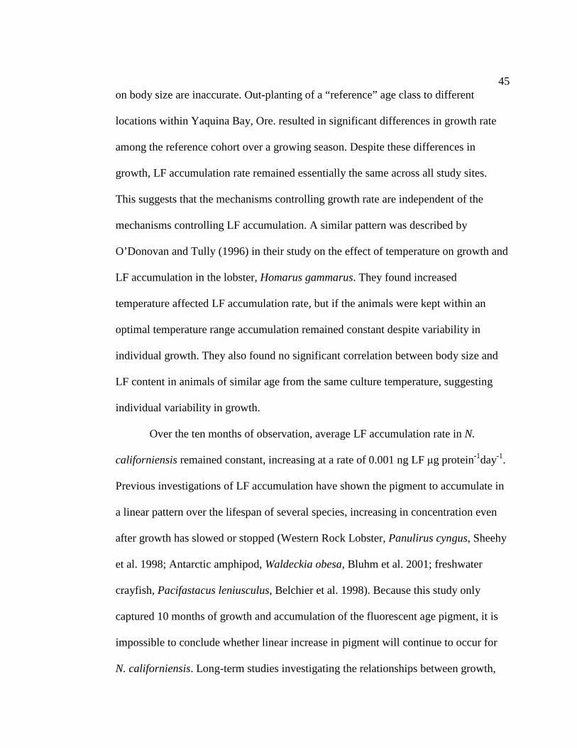
45 on body size are inaccurate. Out-planting of a “reference” age class to different

locations within Yaquina Bay, Ore. resulted in significant differences in growth rate

among the reference cohort over a growing season. Despite these differences in

growth, LF accumulation rate remained essentially the same across all study sites.

This suggests that the mechanisms controlling growth rate are independent of the

mechanisms controlling LF accumulation. A similar pattern was described by

O’Donovan and Tully (1996) in their study on the effect of temperature on growth and

LF accumulation in the lobster, Homarus gammarus. They found increased

temperature affected LF accumulation rate, but if the animals were kept within an

optimal temperature range accumulation remained constant despite variability in

individual growth. They also found no significant correlation between body size and

LF content in animals of similar age from the same culture temperature, suggesting

individual variability in growth.

Over the ten months of observation, average LF accumulation rate in N.

californiensis remained constant, increasing at a rate of 0.001 ng LF µg protein-1day-1.

Previous investigations of LF accumulation have shown the pigment to accumulate in

a linear pattern over the lifespan of several species, increasing in concentration even

after growth has slowed or stopped (Western Rock Lobster, Panulirus cyngus, Sheehy

et al. 1998; Antarctic amphipod, Waldeckia obesa, Bluhm et al. 2001; freshwater

crayfish, Pacifastacus leniusculus, Belchier et al. 1998). Because this study only

captured 10 months of growth and accumulation of the fluorescent age pigment, it is

impossible to conclude whether linear increase in pigment will continue to occur for

N. californiensis. Long-term studies investigating the relationships between growth,

46 LF accumulation and longevity of the ghost shrimp is necessary to develop models for

predicting age based on LF index over this species’ lifespan.

The rapid deviation in average body size of shrimp transplanted to different

sites in this study leads to some interesting questions regarding growth of these

deposit-feeding organisms. Temperature and food supply are the most important

factors controlling crustacean growth (Hartnoll 1982; Hartnoll 2001). For

poikilothermic animals who gain thermal energy from the surrounding environment,

elevated temperatures may cause an increase in metabolism and therefore increase

growth rate. Seasonal oscillation in growth rate in relation to water temperature is well

documented in a number of crustaceans (Ju et al. 1999; Hartnoll 2001; Kodama et al.

2006). Since LF is a biochemical age marker, accumulation rate of LF reflects

metabolic rate of the animal (Sohol 1981; Sheehy et al 1995). In the current study,

average LF index did not vary significantly among study sites. Although animals at

SWI experienced a lower mean temperature during the growing season (July – Oct)

than the other two sites (Figure 2.8), the average body size at that site increased 30.5%

over the ten months of the study. In contrast, average monthly temperature at IFL was

not different from temperature at IFH yet there was a significant increase in body size

at IFL relative to IFH. If temperature affected metabolic rate in N. californiensis, a

significant deviation in average LF index would have been observed between the

Seawall Island and Idaho Flats study sites over the ten month study. Newell (1969)

reviewed the effect of fluctuation in temperature on the metabolism of intertidal

invertebrates and concluded that metabolic rate is relatively independent of

temperature for most intertidal species. Similarly, Wahle et al. (1996) showed that

47 metabolic rate in the lobster Homarus americanus was not reflected in growth and

suggested that energy may be reallocated from growth to other physiological functions

while maintaining an overall static metabolic rate. Clearly, the intertidal sites N.

californiensis inhabit encounter a wide range of thermal conditions throughout the

year and these animals have adapted by adopting temperature-independent metabolic

pathways.

While temperature may not be a major factor influencing growth in N.

californiensis, food supply and density dependence likely play greater roles. On the

Oregon coast, summertime ocean conditions are characterized by strong coastal

upwelling. Cold, nutrient-rich, upwelled water intrudes into the estuary, delivering

nutrients and phytoplankton and fueling production (Roegner and Shanks 2001;

Hickey and Banas 2003; Brown et al. 2007). In this study, the SWI site was located

lowest in the intertidal and closest to the mouth of the estuary. Thus, animals

inhabiting SWI were presumably exposed to the coastal marine water mass for longer

periods than those at IFL and especially at IFH. This would have resulted in greater

food resource availability during the growing season. Under starving conditions,

crustaceans have been shown to produce a hormone that inhibits molting (Keller and

Orth 1990). Low food supply coupled with high densities of shrimp at the IFH site

may explain the absence of significant growth over the ten month study. In-depth

studies of water and sediment nutrient content in relation to growth rate are necessary

to clarify the role of food supply on growth in N. californiensis. Further investigation

into the effect of intraspecific competition may also provide valuable information

48 regarding growth rate in these deposit-feeding shrimp which are generally found in

dense populations.

Conclusions

Analysis of extractable LF shows great promise for determining age in the

ghost shrimp, N. californiensis. Data presented in this study show that the biochemical

extraction technique, modified from Ju et al. (1999), is a practical method for

quantifying age-pigment concentration in brain tissue samples of N. californiensis.

Maximum fluorescence intensity for LF in N. californiensis is achieved at 615 nm

(yellow-orange) when excited at 281 nm (ultraviolet) and freezing as a method of

preservation caused significant increase in fluorescence intensity of LF. It is

recommended that all samples be treated the same in aging studies using analysis of

extractable LF, either processing samples fresh or freezing the animal prior to LF

analysis.

Body size does not reflect chronological age in N. californiensis and therefore

analysis of LF provides a more accurate estimate of true age. In addition, LF index

may provide a measure for comparison among populations within and between

estuaries on relevant spatial scales. In this study, growth varied markedly by location

within the estuary while LF, a physiological marker reflecting metabolic rate of the

animal remained constant. This suggests that food supply or perhaps density, but not

temperature, influenced shrimp growth. Further studies into growth, LF accumulation,

and longevity of N. californiensis are needed to develop models for predicting age in

wild populations. Population analyses using LF as an index of age should be used to

49 develop more robust population dynamics models where traditional length-based

methods of age determination have proven inaccurate. This would facilitate

advancement in the understanding of ghost shrimp population biology and contribute

to the overall body of knowledge regarding age and growth in crustaceans.

LITERATURE CITED Bhattacharya, C.G. 1967. A simple method of resolution of a distribution into Gaussian components. Biometrics 23:115-135. Belchier, M., L. Edsman, M.R.J. Sheehy and P.M.J. Shelton. 1998. Estimating age and growth in long-lived temperate freshwater crayfish using lipofuscin. Freshwater Biology 39:439-446. Bird. E.M. 1982. Population dynamics of thalassinidean shrimps and community effects through sediment modification. PhD dissertation, University of Maryland, College Park, Maryland. Pp.1-140. Bluhm, B.A., T. Brey and M. Klages. 2001. The autofluorescent age pigment lipofuscin: key to age, growth and productivity of the Antarctic amphipod Waldeckia obesa (Chevreux, 1905). Journal of Experimental Marine Biology and Ecology 258:215-235. Boulton, M., M. Rózanowska, B. Rózanowski and T. Wiess. 2004. The photoreactivity of ocular lipofuscin. Photochemical and Photobiological Sciences 3:759-764. Brown, C.A., W.G. Nelson, B.L. Boese, T.H. DeWitt, P.M. Eldridge, J.E. Kaldy, H. Lee II, J. H. Power and D.R. Young. 2007. An approach to developing nutrient criteria for Pacific Northwest estuaries: A case study of Yaquina Estuary, Oregon. USEPA Office of Research and Development, National Health and Environmental Effects Laboratory, Western Ecology Division. EPA/600/R- 07/046. Pp.169. Clarke, A., M.A. Kendall and D.J. Gore. 1990. The accumulation of fluorescent age pigments in the trochid gastropod Monodonta lineate. Journal of Experimental Marine Biology and Ecology 144:185-204. Dumbauld, B.R., D.A. Armstrong and K.L. Feldman.1996. Life-history of two sympatric thalassinidean shrimps, Neotrypaea californeisis and Upogebia

50 pugettensis, with implications for oyster culture. Journal of Crustacean Biology 16(4): 689-708. Dumbauld, B.R., K.M. Brooks and M.H. Posey. 2001. Response of an estuarine benthic community to application of the pesticide carbaryl and cultivation of pacific oysters (Crassostrea gigas) in Willapa Bay, Washington. Marine Pollution Bulletin 42: 826-844. Dumbauld, B.R., S. Booth, D. Cheney, A. Suhrbier, and H. Beltran. 2006. An integrated pest management program for burrowing shrimp control in oyster aquaculture. Aquaculture 261: 976-992. Ettershank, G., I. Macdonnell and R. Croft. 1983. The accumulation of age pigment by the fleshfly Sarcophaga bullata Parker (Diptera:Sarcophagidae) Australian Journal of Zoology 31:131-138. Feldman, K.L., D.A. Armstrong, B.R Dumbauld, T.H. Dewitt and D.C. Doty. 2000. Oysters, crabs, and burrowing shrimp: Review of an environmental conflict over aquatic resources and pesticide use in Washington State’s (USA) coastal estuaries. Estuaries 23(2):141-176. Gayanilo, F.C., P. Sparre and D. Pauly. FAO-ICLARM Stock assessment tools II (FiSAT II). Revised Version. 2005. FAO, Rome, Italy. Gulland, J.A. and A.A. Rosenberg. 1992. A review of length-based approaches to assessing fish stocks. FAO Fisheries Technical Paper 323. Rome, FAO. 100 pp. Hartnoll, R.G. 1982. Growth. In Bliss, D.E. and L.G. Abele (eds), The biology of Crustacea, 2, Embryology, Morphology and Genetics. Academic Press, New York. Pp 111-196. Hartnoll, R.G. 2001. Growth in Crustacea – twenty years on. Hydobiologia 449:111- 122. Harvey, H.R., D. H. Secor and S-J Ju. 2008. The use of extractable lipofuscin for age determination of crustaceans: reply to Sheehy (2008). Marine Ecology Progress Series 353: 307-311. Hicky, B.M. and N.S. Banas. 2003. Oceanography of the U.S. Pacific Northwest coastal ocean and estuaries with application to coastal ecology. Estuaries 26: 1010-1031.

51 Hill, K.T., and C.T. Womersley. 1991. Critical aspects of fluorescent age – pigment methodologies: modification for accurate age assessment in aquatic organisms. Marine Biology 109:1-11. Ju, S-J., D.H. Secor, and H.R. Harvey. 1999. Use of extractable lipofuscin for age determination of the blue crab, Callinectes sapidus. Marine Ecology Progress Series 185:171-179. Ju, S-J. 2000. Development and application of biochemical approaches to understanding age and growth in crustaceans. PhD thesis, University of Maryland, College Park, MD. Ju, S-J., D.H. Secor and H.R. Harvey. 2001. Growth rate variability and lipofuscin accumulation in the blue crab Callinectes sapidus. Marine Ecology Progress Series 224:197-205. Keller, R. and H.-P. Orth. 1990. Hyperglycemic neuropeptided in crustaceans. In Scanes, C.G. and M.H. Stetson (eds), Progress in Comparative Endocrinology. John Wiley and Sons, New York: 265 – 271. Kodama, K., H. Shiraishi, M. Morita, and T. Horiguchi. 2006. Verification of lipofuscin-based crustacean ageing: seasonality of lipofuscin accumulation in the stomatopod Oratosquilla oratoria in relation to water temperature. Marine Biology 150:131-140. MacGinite, G.E. 1934. The natural history of Callianassa californiensis Dana. American Midland Naturalist 15(2):166-177. Maggi, V. and P.N. Riddle. 1965. Histochemisty of tissue culture cells: a study of the effects of freezing and of some fixatives. Journal of Histochemisty and cytochemisty 13(5):310-317. Medina, A., Y. Vila, C, Megina, I. Sobrino and F. Ramos. 2000. A histological study of the age-pigment, lipofuscin, in dendrobranchiate shrimp brains. Journal of Crustacean Biology 20(3):423-430. Newell, R.C. 1969. Effect of fluctuations in temperature on the metabolism of intertidal invertebrates. American Zoologist 9:293-307. Nicol, S. 1987. Some limitations on the use of the lipofuscin ageing technique. Marine Biology 93:609-614.

52 O’Donovan, V. and O. Tully. 1996. lipofuscin (age pigment) as an index of crustacean age: correlation with age , temperature and body size in cultured juvenile Homarus gammarus L. Journal of Experimental Marine Biology and Ecology 207:1-14. Posey , M.H. 1986. Changes in a benthic community associated with dense beds of a burrowing deposit feeder, Callianassa californiensis. Marine Ecology Progress Series 31:15-22. Posey, M.H. 1987. Effects of lowered salinity on activity of the ghost shrimp Callianassa californiensis. Northwest Science 61(2):93-96. Prentø, P. 1997. The effects of freezing, storage, and thawing on cell compartment integrity and ultrastructure. Histochemisty and Cell Biology 108:543-547. Roegner, G.C. and A.L. Shanks. 2001. Import of coastally-derived chlorophyll a to South Slough, Oregon. Estuaries 24:224-256. Sheehy, M.R.J. 1989. Crustacean brain lipofuscin: an examination of the morphological pigment in the fresh-water crayfish Cherax cuspidatus (Parastacidae). Journal of Crustacean Biology 9(3): 387-391. Sheehy, M.R.J. 1996. Quantitative comparison of in situ lipofuscin concentration with soluble autofluorescence intensity in the crustacean brain. Experimental Gerontology 31:421-432. Sheehy, M.R.J. 2008. Questioning the use of biochemical extraction to measure lipofuscin for age determination of crabs: Comment of Ju et al. (1999, 2001). Marine Ecology Progress Series 353:303-306. Sheehy, M.R.J., J.G. Greenwood and D.R. Fielder. 1994. More accurate chronological age determination of crustaceans from field situations using the physiological age marker, lipofuscin. Marine Biology 121: 237-254. Sheehy, M.R.J., E. Cameron, G. Marsden and J. McGrath. 1995. Age structure of female giant tiger prawns Penaus monodon as indicated by neuronal lipofuscin concentration. Marine Ecology Progress Series 117:59-63. Sheehy, M.R.J., N. Caputi, C. Chubb and M. Belchier. 1998. Use of lipofuscin for resolving cohorts of western rock lobster (Panulirus Cygnus).Canadian Journal of Fisheries and Aquatic Sciences 55:925-936.

53 Smith, P. K., R. I. Krohn, G. T. Hermanson, A.vK. Mallia, A. K. Gartner, M. D. Povenzano, E.K. Fujimoto, N. M. Goeke, B.J. Olson and D.C. Klenk. 1985. Measurement of protein using bichoninic acid. Analytical Biochemistry 150:76-85. Sohol, R.S. 1981. Relationship between metabolic rate, lipofuscin accumulation, and lysosomal enzyme activity during aging in the adult housefly, Musca domestica. Experimental Gerontology 16: 347-355. Vernet, M., J.R. Hunter and R.D. Vetter. 1988. Accumulation of age pigments (lipofuscin) in two cold water fishes. Fishery Bulletin 86: 401-407. Wahle, R.A., O. Tully and V. O’Donovan. 1996. Lipofuscin as an indicator of age in crustaceans: analysis of the pigment in the American lobster Homarus americanus. Marine Ecology Progress Series 138:117-123 Yin D. and U. T. Brunk. 1991. Microfluorometric and fluorometric lipofuscin spectral discrepancies: a concentration-dependant metachromatic effect? Mechanisms of Ageing and Development 59: 95-109. Yin, D. 1996. Biochemical basis of lipofuscin, ceroid, and age pigment-like fluorophores. Free Radical Biology and Medicine 21:871-888.

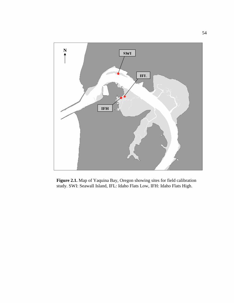
54

IFH

IFL

SWI N

Figure 2.1. Map of Yaquina Bay, Oregon showing sites for field calibration study. SWI: Seawall Island, IFL: Idaho Flats Low, IFH: Idaho Flats High.

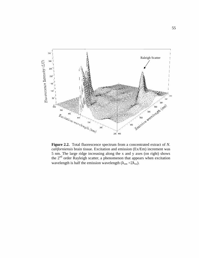
55

Figure 2.2. Total fluorescence spectrum from a concentrated extract of N. californiensis brain tissue. Excitation and emission (Ex/Em) increment was 5 nm. The large ridge increasing along the x and y axes (on right) shows the 2nd order Rayleigh scatter, a phenomenon that appears when excitation wavelength is half the emission wavelength (λem =2λex).

Raleigh Scatter

56

Figure 2.3. Excitation spectrum of brain tissue extract along a single emission wavelength. The major peak at 310 nm excitation represents Rayleigh scatter. Other Ex/Em maxima represent potential fluorescent age related products in extract. Major peaks of fluorescence occur at Ex/Em 281/615, 464/615, 273/515, 367/515, and 450/515.

Excitation Wavelength (nm)

250 300 350 400 450 500 550

LU

0

20

40

60

80

100

120

140

160

615 emission 515 emission

Rayleigh Scatter

57

Figure 2.4. Regression results of pooled LF index data from all three study sites in Yaquina Bay showing relationship of LF index to time. Regression lines represent LF indices calculated from two major excitation/emission maxima present in tissue extract of N. californiensis. LF A – 281/615, LF B – 273/515. LF A represents the age-related fluorescent pigment. Error bars show standard deviation.

Day

0 50 100 150 200 250 300 350

LF in

dex

(ng/

ug)

0.0

0.2

0.4

0.6

0.8

1.0

1.2

LF ALF B

58

2+

2+

1+

Female

Male

n = 191

n = 97

Figure 2.5. Results of Modal Progression Analysis (MPA) of length-frequency histograms of male and female N. californiensis from Idaho Flats. Animals were collected on 4/27/2007. These data were used to determine size range of age 2+ “reference age class” used in calibration study.

59

Day

0 50 100 150 200 250 300 350

Car

apac

e Le

ngth

(m

m)

4

6

8

10

12

14

SWI

IFL

IFH

Figure 2.6. Results of multiple linear regression analysis showing difference in growth rate of a cohort planted across three sites in Yaquina Bay, Ore. Each data point represents the body size measurement for an individual shrimp at each site for each sample period. The initial sample (t = 0) was distributed among all sites to monitor growth overtime. SWI exhibited highest growth over the ten months of the study. IFL was intermediate and IFH showed little increase in body size. Comparison of regression lines indicates statistically different slopes for each site.

60

Figure 2.7. Results of multiple linear regression analysis showing positive relationship between LF index and time (day) from three sites in Yaquina Bay, Ore. Each data point represents the LF index value (LF A) for an individual shrimp at a specific site for each sample period. Slopes of regression lines were not significantly different from each other at the 95% confidence level.

Day

0 50 100 150 200 250 300 350

LF in

dex

(ng/

ug)

0.0

0.2

0.4

0.6

0.8

1.0

1.2SWI

ILH

IFH

INITAL

61

Figure 2.8. Average monthly temperature at three study sites in Yaquina Bay, Oregon. Error bars represent standard deviation in mean monthly temperature.

Yaquina Bay Temperature

Month

Jul Aug Sep Oct Nov Dec Jan Feb Mar Apr

Tem

pera

ture

(de

g C

)

2

4

6

8

10

12

14

16

18

20

22

IFH IFL SWI

62

Tem

per

atu

re (

deg

C)

10

12

14

16

18

20

22

24

IFH IFL SWI

7/15/2007 7/16/2007

06:00 12:00 18:00 0:00 06:00 12:00 18:00 0:00

Figure 2.9. Temperature fluctuations experienced at all three study sites over two tidal cycles in July 2007. Data represent hourly temperature readings taken 10 cm below the sediment surface on 7/15/07 and 7/16/07. Maximum change in temperature was 9.49 º C at IFH.

63

Correlation of Fluorescence Maxima (N = 51)

Ex/Em 1 2 3 4 5 1. 463/615 -

2. 281/615 0.998* -

3. 450/515 -0.132 -0.095 -

4. 367/515 -0.118 -0.081 1.00* -

5. 273/515 -0.128 -0.091 1.00* 1.00* -

Table 2.1. Results from Pearson’s correlation between fluorescence intensities obtained from all five Ex/Em maxima observed in N. californiensis. *p < 0.001.

64

Regression Slope ± SE Intercept ± SE R2 P

LF A vs. Time 0.0010 ± 0.0001 0.386 ± 0.019 0.37 < 0.001

LF B vs. Time -0.0004 ± 0.0002 0.355 ± 0.034 0.04 0.027

Table 2.2. Results of regression analysis between LF index and time for two major Ex/Em maxima found in brain tissue of N. californiensis. LF A represents LF index (ng µg-1) calculated from Ex/Em 281/615 (n=166). LF B represents LF index (ng µg-1) calculated from Ex/Em 273/515 (n=98). LF A is positively correlated with time indicating that it is a fluorescent age product.

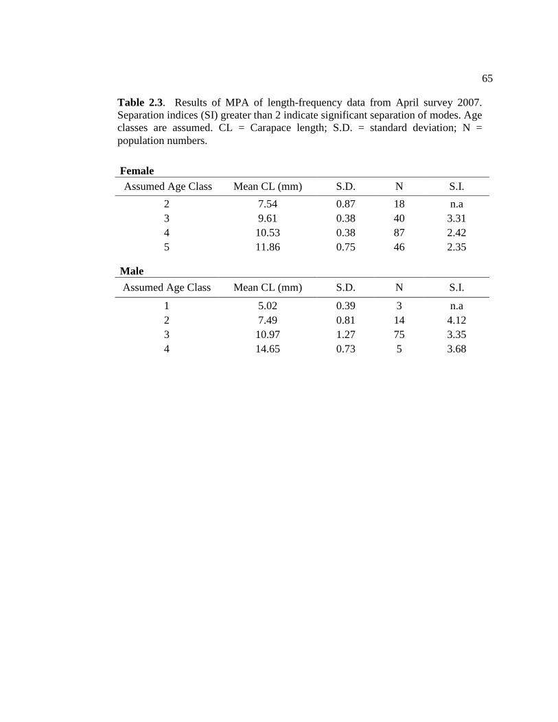
65

Female

Assumed Age Class Mean CL (mm) S.D. N S.I.

2 7.54 0.87 18 n.a 3 9.61 0.38 40 3.31 4 10.53 0.38 87 2.42 5 11.86 0.75 46 2.35

Male

Assumed Age Class Mean CL (mm) S.D. N S.I.

1 5.02 0.39 3 n.a 2 7.49 0.81 14 4.12 3 10.97 1.27 75 3.35 4 14.65 0.73 5 3.68

Table 2.3. Results of MPA of length-frequency data from April survey 2007. Separation indices (SI) greater than 2 indicate significant separation of modes. Age classes are assumed. CL = Carapace length; S.D. = standard deviation; N = population numbers.

66

Regression Slope ± SE Intercept ± SE R2 P n

Size vs. Time SWI 0.0076 ± 0.0006 7.55 ± 0.069 0.48 < 0.001 161 IFH 0.0008 ± 0.0003 7.48 ± 0.035 0.04 0.005 139 IFL 0.0047 ± 0.0005 7.60 ± 0.072 0.34 < 0.001 199 Z < 0.001

LF vs. Time SWI 0.0008 ± 0.0002 0.376 ± 0.027 0.23 < 0.001 62 IFH 0.0011 ± 0.0001 0.383 ± 0.021 0.47 < 0.001 72 IFL 0.0013 ± 0.0002 0.376 ± 0.024 0.51 < 0.001 88 Z NS

Table 2.4. Results of regression analysis examining effects of time and site on body size (CL (mm)) and LF index (ng LF µg protein-1). Z, slope comparison between sites. NS, not significant (p>0.05). SWI = Seawall Island; IFH = Idaho Flats High; IFL = Idaho Flats Low.

67

Treatment Average CL LF A LF B n Sign. Fresh 11.54 ± 1.30 13.06 ± 4.40 2.75 ±1.69 45 a

Frozen 2 weeks 11.44 ± 1.28 24.09 ± 7.37 43.10 ± 29.8 43 b

Frozen 6 months 11.20 ± 1.20 21.40 ± 7.03 36.57 ± 20.0 45 b

Table 2.5. Results of One-Way ANOVA testing for difference in average LF concentration from samples processed fresh and those previously frozen. n = number of samples in a treatment group; Sign. = pair-wise comparison of LF concentration among treatment groups. Treatments with the same letter are not significantly different from each other.

68 Chapter 3: Assessment of population age structure for the ghost shrimp, Neotrypaea californiensis, in West Coast estuaries using extractable lipofuscin as an age biomarker

ABSTRACT

Determining accurate age estimates in crustaceans is inherently difficult because they

lack hard structures with growth increments that can be used for ageing. Physical

measurements such as body length are generally used to identify age classes.

However, several studies have shown that length is a poor predictor of true age. Age

determination using the autofluorescent age marker, lipofuscin (LF), has recently

gained popularity with ecologists and managers studying crustacean population

dynamics and has been effective in resolving age structure in a number of ecologically

and economically important species. Extractable LF was used to determine age

structures for three populations of the burrowing shrimp, Neotrypaea californiensis, in

West Coast estuaries and compared to age structures obtained from traditional length-

based methods. Assessments were conducted in spring and fall of 2007. Analysis of

LF indicated up to 13 age classes present in shrimp populations, an estimate much

higher than estimates in assessments using carapace length measurements. LF-based

age classes were composed of a broad range of sizes, suggesting that growth varies

within populations. No significant difference in LF accumulation rate was observed

among three study sites. Average LF index increased 0.20 ng LF µg protein-1 between

April and October. Comparison of mean size-at-age among populations in Oregon and

Washington showed growth rate varied spatially. Animals from the Palix River in

Willapa Bay were 43% larger than animals of the same age from Yaquina Bay,

69 suggesting that local environment influences growth. Site-specific environmental

factors like food availability, population density and tidal elevation may control

individual and population growth patterns. Linear and Von Bertalanffy growth models

inadequately described the relationship of size and age for all populations assessed.

Data obtained in this study provides evidence that lipofuscin-based aging is more

accurate than length-based methods for the ghost shrimp, N. californiensis. The age-

model presented here can be used to develop population models to advance

understanding of the population biology of this species.

70 INTRODUCTION Obtaining accurate age estimates in wild crustacean populations has posed a

problem for scientists studying population dynamics. Age is an important parameter

used to develop fishery resource models and calculate population parameters such as

growth rate, age-at-maturity, mortality and fecundity. Unlike finfish and molluscs,

crustaceans shed all hard parts with each molt and do not retain any morphological

evidence of age throughout their lifespan. Traditionally, morphometric measurements,

such as carapace length or width, have been used as a surrogate for age in crustaceans.

However, individual variation in growth rate has made it difficult to distinguish

cohorts based on body size data (Parsons and Fréchette, 1989). Several studies have

shown that growth rates in crustaceans are influenced by a wide array of biotic (e.g.,

density dependant) and abiotic (e.g., environmental) factors (Newman and Pollock

1974; Klein Breteler 1975; Ra’anan and Cohen 1985; Hartnoll 2001). Given that

growth rates can vary, building age-based population models and empirically deriving

population parameters from length-based estimates of age adds significant sources of

error when assessing crustacean populations for management and conservation

applications.

A recent alternative approach to age determination using the auto-fluorescent

age pigment, lipofuscin (LF), has been successfully used to age a number of

crustacean species. The pigment occurs widely in vertebrate and invertebrate taxa and

is known to increase in concentration with age (Sohol 1981b; Sheehy 1990; Yin 1996;

Porta 2002). LF is formed as a by-product of cellular degeneration and is retained

within cells throughout the animals’ lifespan (Sohol 1981a). The amount of LF in

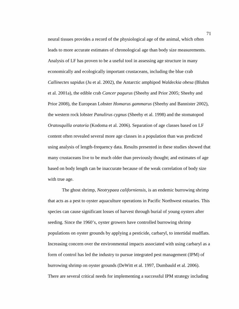
71 neural tissues provides a record of the physiological age of the animal, which often

leads to more accurate estimates of chronological age than body size measurements.

Analysis of LF has proven to be a useful tool in assessing age structure in many

economically and ecologically important crustaceans, including the blue crab

Callinectes sapidus (Ju et al. 2002), the Antarctic amphipod Waldeckia obesa (Bluhm

et al. 2001a), the edible crab Cancer pagurus (Sheehy and Prior 2005; Sheehy and

Prior 2008), the European Lobster Homarus gammarus (Sheehy and Bannister 2002),

the western rock lobster Panulirus cygnus (Sheehy et al. 1998) and the stomatopod

Oratosquilla oratoria (Kodoma et al. 2006). Separation of age classes based on LF

content often revealed several more age classes in a population than was predicted

using analysis of length-frequency data. Results presented in these studies showed that

many crustaceans live to be much older than previously thought; and estimates of age

based on body length can be inaccurate because of the weak correlation of body size

with true age.

The ghost shrimp, Neotrypaea californiensis, is an endemic burrowing shrimp

that acts as a pest to oyster aquaculture operations in Pacific Northwest estuaries. This

species can cause significant losses of harvest through burial of young oysters after

seeding. Since the 1960’s, oyster growers have controlled burrowing shrimp

populations on oyster grounds by applying a pesticide, carbaryl, to intertidal mudflats.

Increasing concern over the environmental impacts associated with using carbaryl as a

form of control has led the industry to pursue integrated pest management (IPM) of

burrowing shrimp on oyster grounds (DeWitt et al. 1997, Dumbauld et al. 2006).

There are several critical needs for implementing a successful IPM strategy including

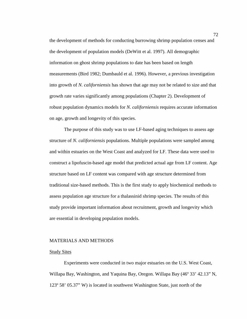
72 the development of methods for conducting burrowing shrimp population censes and

the development of population models (DeWitt et al. 1997). All demographic

information on ghost shrimp populations to date has been based on length

measurements (Bird 1982; Dumbauld et al. 1996). However, a previous investigation

into growth of N. californiensis has shown that age may not be related to size and that

growth rate varies significantly among populations (Chapter 2). Development of

robust population dynamics models for N. californiensis requires accurate information

on age, growth and longevity of this species.

The purpose of this study was to use LF-based aging techniques to assess age

structure of N. californiensis populations. Multiple populations were sampled among

and within estuaries on the West Coast and analyzed for LF. These data were used to

construct a lipofuscin-based age model that predicted actual age from LF content. Age

structure based on LF content was compared with age structure determined from

traditional size-based methods. This is the first study to apply biochemical methods to

assess population age structure for a thalassinid shrimp species. The results of this

study provide important information about recruitment, growth and longevity which

are essential in developing population models.

MATERIALS AND METHODS

Study Sites

Experiments were conducted in two major estuaries on the U.S. West Coast,

Willapa Bay, Washington, and Yaquina Bay, Oregon. Willapa Bay (46º 33’ 42.13” N,

123º 58’ 05.37” W) is located in southwest Washington State, just north of the

73 Columbia River. It is classified as a coastal-plain estuary, with a connection to the

highly active eastern boundary of the Pacific Ocean and the northern reach of the

California Current System (Hickey 1989). The bay encompasses a total area of 260

km2 at mean high water and is relatively shallow with less than 15% being deeper than

7m (Hedgeperth and Obrebski 1981). At mean low tide, 86 km2 of intertidal area is

exposed (Dumbauld unpub.). Tides are mixed-semidiurnal with a range of 4 meters.

Sediments near the mouth of the bay are mainly composed of sand and become siltier

with increased organic debris deposited from riverine sources with increasing distance

from the mouth.

Willapa Bay is a major site for oyster aquaculture on the West Coast,

producing approximately 10% of the commercial oysters harvested in the U.S.

(Reusink et al. 2006). The bay is comprised of a number of different habitat types,

including marshes, seagrass, oyster reefs and mudflats that provide important nursery

grounds for many commercially important species, such as Dungeness crab and

salmon (Murphy et al. 2000; Hosack et al. 2006). Dense populations of the ghost

shrimp N. californiensis occur in sandy sediment throughout the bay. Ghost shrimp

habitat makes up about 13% of the total intertidal area of the bay with most of the

populations occurring near the mouth, where marine influence is highest (Dumbauld

and McCoy unpublished).

Yaquina Bay (44º 37’ 08.07” N, 124º 02’ 29.68” W) is located on the central

Oregon Coast and is also classified as a coastal plain or drowned-river-valley type

estuary. The Yaquina River is the primary tributary which feeds into the bay. The bay

is relatively small, encompassing approximately 17.1 km2 at mean high water (Shirzad

74 et al. 1988). The average tidal range of the bay is 2 meters, exposing 8.2 km2 of tide

flat at mean low water (Dumbauld and McCoy unpub; Percy 1974). Yaquina Bay

varies between a partially-mixed and well-mixed estuary depending on the season

(Burt and McAlister 1959). During months when freshwater input from the Yaquina

River is high, the bay is classified as partially-mixed, with coastal marine water

pushing far beyond the mouth over a tidal cycle. During months when freshwater

input is low, a well-mixed system characterizes the bay. Dense populations of

thalassind shrimps are found across the intertidal area of the bay. Population density

can exceed 500 shrimp m-2 in some locations (DeWitt et al. 2004).

Three sites were selected for demographic assessments, two in Willapa Bay

and one in Yaquina Bay (Figure 3.1). Sites were selected because large populations of

ghost shrimp with different average sizes are present at each location (Figure 3.2) and

all three sites are surveyed yearly as part of a long-term monitoring program. The two

sites selected in Willapa Bay represent different levels of marine influence and tidal

circulation patterns. The Palix River (PR) site is located near the mouth of the bay (13

km) and receives strong marine influence from coastal waters intruding into the

estuary. Tidal elevation at this site is 1.64 ft. mean lower low water (MLLW) and

average population density is 132 ± 35 individuals m-2. The second site in Willapa Bay

is Middle Island Sands (MIS). MIS is located 27 km from the mouth of the bay.

Average population density at this site is 170 ± 44.2 m-2 and animals at this location

are noticeably smaller than those found to the north at PR. Tidal elevation at MIS is

1.65 ft. MLLW. The third site, Idaho Flats (IF), was selected as the Yaquina Bay

sample site. IF is located high in the intertidal (4.96 ft. MLLW) and shrimp at this site

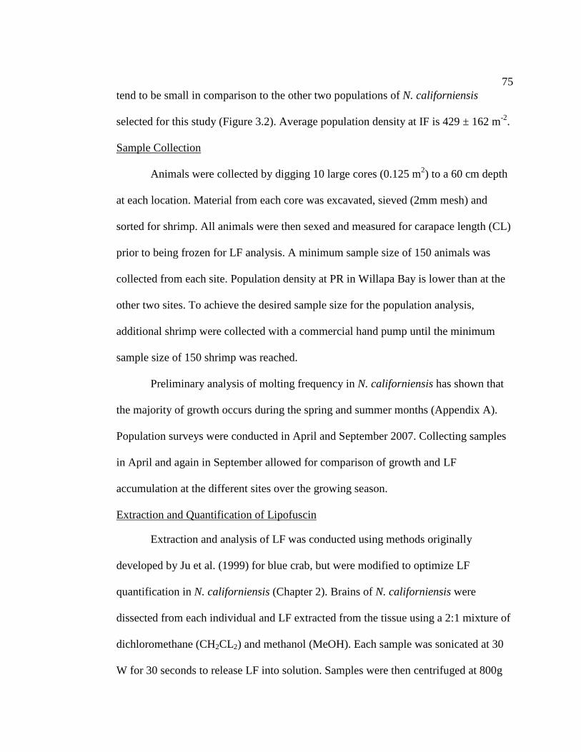
75 tend to be small in comparison to the other two populations of N. californiensis

selected for this study (Figure 3.2). Average population density at IF is 429 ± 162 m-2.

Sample Collection

Animals were collected by digging 10 large cores (0.125 m2) to a 60 cm depth

at each location. Material from each core was excavated, sieved (2mm mesh) and

sorted for shrimp. All animals were then sexed and measured for carapace length (CL)

prior to being frozen for LF analysis. A minimum sample size of 150 animals was

collected from each site. Population density at PR in Willapa Bay is lower than at the

other two sites. To achieve the desired sample size for the population analysis,

additional shrimp were collected with a commercial hand pump until the minimum

sample size of 150 shrimp was reached.

Preliminary analysis of molting frequency in N. californiensis has shown that

the majority of growth occurs during the spring and summer months (Appendix A).

Population surveys were conducted in April and September 2007. Collecting samples

in April and again in September allowed for comparison of growth and LF

accumulation at the different sites over the growing season.

Extraction and Quantification of Lipofuscin

Extraction and analysis of LF was conducted using methods originally

developed by Ju et al. (1999) for blue crab, but were modified to optimize LF

quantification in N. californiensis (Chapter 2). Brains of N. californiensis were

dissected from each individual and LF extracted from the tissue using a 2:1 mixture of

dichloromethane (CH2CL2) and methanol (MeOH). Each sample was sonicated at 30

W for 30 seconds to release LF into solution. Samples were then centrifuged at 800g

76 for 10 minutes to remove cellular debris. Half of the total extract (500µl) was

transferred into a 1 ml amber vial where contents were dried under N2 and re-

dissolved in 250 µl MeOH to be analyzed with an Agilent 1100 scanning fluorescence

detector. Fluorescence intensity was measured with emission wavelength 615 nm

using excitation wavelength 281 nm and recorded with the ChemStation B.03.01

software program (Agilent Technologies, Inc. 2007). LF concentration in each sample

was determined by calibrating fluorescence intensity to a standard curve of quinine

sulfate dissolved in 0.1N H2SO4 (Appendix B). A quantitative measure of LF was

provided by normalizing LF concentration in the sample to the protein content in the

tissue extract. Protein concentration was determined using the bicinchoninic acid

assay (BCA) (Smith et al. 1985). The final measurement was expressed as a protein-

normalized lipofuscin index (ng LF µg protein-1) (Eq. 1). This index was treated as the

dependent variable in all regression analyses.

Equation 1:

LF Index = Extractable LF concentration calibrated verses quinine sulfate (ng ml-1) (ng µg -1) Total protein content (extract and tissue) (µg ml-1)

Statistical Analyses

Potential outliers and strongly influential data points were identified by

conducting an outlier analysis on untransformed data. Regressions of protein

concentration and absolute LF concentration against carapace length showed strong

linear relationships for all three sites (Appendix D). Data points with studentized

residuals greater than the value 4 were removed because it is likely these outlying

points were a result of sample contamination during processing rather than real data

77 values. All least-squares regression analyses were conducted using STATGRAPHICS

Centurion XV (StatPoint Inc. 2005) and Sigma Plot 10.0 (Systat Software Inc. 2006).

The two-sample Kolomogrov-Smirnov (K-S) test for population was used to

determine if LF index and CL frequency distribution differed by sex. Variables that

did not differ significantly between sexes were pooled for Modal Progression Analysis

(MPA; see description below).

Age class identification

Standard frequency histograms were constructed for each sample site using

both CL and LF data from all three sample sites. Class intervals for length-frequency

histograms were specified at 1 mm CL for MIS and PR and 0.75 mm CL for IF.

Animals at IF tended to be smaller than animals at MIS and PR. Selecting a class

interval of 0.75 mm for that site produced the highest number of resolvable modes in

length-frequency histograms without losing too much information from binning data.

Class interval for LF index-frequency distributions was specified at 0.1 ng LF content

µg protein-1 for all three populations. Modal progression analysis (MPA) was

conducted to resolve age structure from both LF and length data. In order to do this,

each frequency distribution was broken into its individual Gaussian components using

Bhattacharya’s method (Bhattacharya 1967) and analyzed for modal separation with

the NORMSEP routine of the FiSAT II statistical software program (FAO- ICLARM

Fish Stock Assessment tools, FAO, Rome, Italy, 2005). The NORMSEP routine

applies the maximum likelihood concept to separate normally distributed components

of frequency distributions (Hasselblad 1966). Modes separated by a minimum

separation index of 2 were considered statistically significant (Gulland and Roseburg

78 1992). Age classes were assigned to modes and calibrated based on average CL and

LF index of the “reference age” 2 + cohort determined in the growth experiments

described in Chapter 2. These age assignments assumed that only one cohort was

produced per year and therefore each mode represented a single year class.

Once age classes were identified from frequency data, age estimates were

assigned to CL and LF index values. For modes that were overlapping, a normal

probability distribution function (Sokal and Rholf, 1995) was used to determine

appropriate cut off values for age assignments. A chi-square test for goodness-of-fit

was used to determine if actual frequencies for estimated age classes conformed to the

frequencies resulting from the MPA. The one-sample K-S test for normality was used

to determine if age groupings were normally distributed for each mode.

Construction of age-based growth model

LF accumulation rate was determined with linear least-squares regression of

LF-estimated age against LF index value. Multiple linear regression was used to test

for significant differences in pigment accumulation among sites for both the spring

and fall samples. Interaction terms were included in multiple regression models to

determine if slopes for each site were significantly different from each other. After

testing for differences among sites, data from all three sites were pooled to build a

single, predictive, age-based model for LF accumulation. The LF accumulation model

was then used to predict age based on LF index value. Linear and Von Bertalanffy

growth models were fit to size-at-age data to determine which model best described

growth for the three populations assessed (Eq.2).

79 Equation 2:

Von Bertalanffy Growth Function (VBGF)

L t = L∞ (1-e-k(t-to)

)

Lt = body length at age t (years)

L∞ = asymptotic body length

k = growth constant

t0 = theoretical age at which Lt = 0 mm

RESULTS

Comparison of size-frequency histograms showed that CL of males and

females were different at all three sites for both sample periods (K-S test; p> 0.05 in

all cases; Figure 3.2). Length data for each sex were treated separately for modal

progression analyses. Comparison of LF index frequency data showed no significant

difference between the sexes and therefore LF indices were pooled for all subsequent

analyses (K-S test, p< 0.05 in all cases).

Five to seven normal distributions were detected in CL-frequency histograms

from the April survey (Figure 3.3 & 3.4; Tables 3.1 – 3.3). Modes were highly

resolved with relatively high separation indices. In some cases, a separation index less

than the critical value of 2 suggested significant overlap in the modes. Progression

analysis of CL data from the September survey detected between 4 and 6 normal

components in each distribution (Figures 3.3 & 3.4; Tables 3.1 – 3.3). All but two

80 cases produced highly resolved modes with separation indices greater than the critical

value of 2.

Modal progression analysis of LF index data revealed several more age classes

than what was determined with analysis of CL data at all sites for both the fall and

spring sample periods (Figure 3.5). At the PR site, nine age classes were observed

from the April sample and ten from the September sample (Table 3.4). Age 4+ in the

spring sample was the only mode that showed significant overlap with the adjacent

age classes. At MIS, seven age classes were observed in both the fall and spring

samples, all of which showed strong separation (Table 3.5). The population at IF

produced the most age groupings, with 13 separate age classes comprising the

frequency distribution from the fall sample (Table 3.6). The spring sample at IF

revealed 10 age classes with statistically significant separation of the groupings.

A lack of young age classes was evident in all three populations assessed. In

several cases, age classes were missing from the overall age structure. These missing

age classes tended to be on the extreme ends of the age distribution. Age classes 1+

and 2 + were weak or missing in all three populations. Age classes 4+ and 5+ were the

strongest at all sites. Numbers-at-age were low in the older age classes, as would be

expected because of natural mortality. At MIS, no significant age groups were found

beyond 7+. The spring sample from MIS showed five individuals with LF index

values greater than 1.5 ng µg-1 (Figures 3.5). These animals did not form groups in the

MPA but age estimates calculated with the LF-based age model indicated animals up

to 13 years old in the sample. At IF, age classes 1+ and 9+ were missing from the

81 spring sample and age groupings and 2+ and 12+ were missing from the fall sample

(Figure 3.5; Table 3.6).

LF index-frequency histograms were used to track increases in LF indices from

spring to fall (Table 3.7). At PR, LF index increased an average of 0.20 ± 0.07 ng ug-1

over the summer growing season. LF index increased 0.18 ± 0.04 ng ug-1 and 0.16 ±

0.07 ng ug-1 at MIS and IF respectively. Regression of LF index with estimated age

showed a strong linear trend in LF accumulation in the three populations for both the

spring and fall samples (Figure 3.6; Table 3.8). Multiple linear regression analysis of

spring survey data showed that the slopes and intercepts produced from the three sites

were not significantly different from each other so all LF index-at-age data were

pooled for spring. A multiple linear regression analysis of fall survey data showed site

to be a significant factor but slopes were not significantly different when compared

among sites (Table 3.8). Data were pooled to estimated average increase in LF

between sample periods. Comparison of regression intercepts showed that LF index

increased an average of 0.20 ng ug-1 over the growing season (Figure 3.7). This

corresponds to an average accumulation rate of 0.0012 ng LF µg protein -1 day-1 over

the 167 days between the spring and fall surveys.

Comparing LF-based age estimates to those determined from analysis of CL

data showed that size-at-age varies within populations. When LF-frequency

histograms from the April survey collection were divided into size classes as

determined from MPA of CL, each mode was composed of animals from a number of

different size classes (Figure 3.8). The largest animals at PR were grouped in age 7+

based on CL, but these animals were actually in the age 4+ age class as determined

82 from the LF index value. Conversely, a number of small animals (size groups 2+ and

3+ from CL) were grouped with older age classes determined from LF indices.

Variation in size-at-age was observed for all three populations sampled.

Pooled data from the April survey were used to develop a single LF-based

model for predicting age in N. californiensis (Figure 3.9). The resulting model showed

a strong correlation of the dependant variable, LF index, to the independent variable,

LF-estimated age (R2 = 0.92, d.f. = 1, n = 443, p < 0.001 ) (Eq. 3). This model was

used to calculate LF-based age estimates for all animals collected in the spring survey

and correlate body size with actual age at each site.

Equation 3:

LF index (ng µg-1) = 0.21* Age (yrs) – 0.056

Neither growth model fit size-at-age data well. The linear model resulted in

non-significant correlations of the variables (CL and LF-estimated age) for both sexes

(Table 3.9; p>0.05 in all cases). The Von Bertalanffy growth function (VBGF) was

also insufficient in correlating body size to age (Figure 3.10; Table 3.10). Size-at-age

data from PR produced a significant model when fit to the VBGF, however a weak

correlation coefficient suggested a poor fit of the model to the data (p = 0.002, r2 =

0.10). The asymptotic length and growth coefficients from the three populations

assessed varied greatly. At IF in Yaquina Bay, the asymptotic length was 10.4 mm.

This value was 43% smaller than what was observed for the PR population in Willapa

Bay (L∞ = 18.5). The population at MIS showed an intermediate asymptotic length

(L∞ = 14.8).

83 DISCUSSION

The results of this study clearly show that N. californiensis is a long-lived

species that can exhibit variable growth rates within and among estuarine populations.

LF-based age estimates determined with MPA of LF index data revealed clear

differences in mean size-at-age when comparing multiple populations of ghost shrimp

across two estuaries. In addition, growth rate was shown to vary within a given

population, resulting in a wide range of sizes for a single age class. Data presented in

this study confirms the hypotheses that a) size is not necessarily related to age and b)

traditional methods of age determination based on body length can introduce

significant sources of error in estimating age in N. californiensis.

Until now, much has remained unknown about the longevity of N.

californiensis. Early studies investigating the ecology of the ghost shrimp led to the

belief that it was a long-lived species, possibly living up to 10 or more years of age

(MacGinitie 1935). MacGinite (1934) suggested that the rare occurrence of juveniles

in Elkhorn Slough near Monterey Bay, California, combined with little to no year

class groupings among individuals and low mortality of established adults, was

evidence that the species was long-lived. More recent life history studies which used

size frequency data to estimate the number of age classes in a population, suggested

the animal lives to be 3 to 5 years old (Bird 1982; Dumbauld et al. 1996). In the

current study, assessment of population age structure using analysis of LF as an age

biomarker was successful in resolving up to 13 separate age classes in Yaquina Bay

and 9 age classes in Willapa Bay. These results support the earlier speculation that the

species can live up to ten or more years.

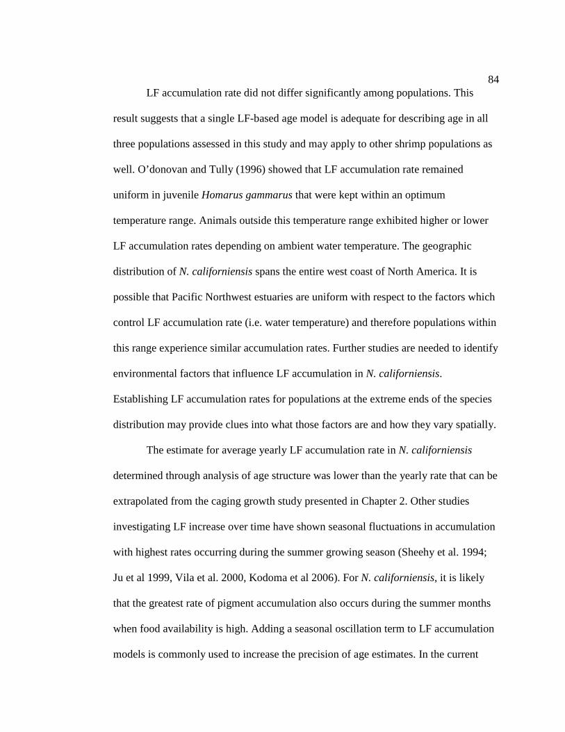
84 LF accumulation rate did not differ significantly among populations. This

result suggests that a single LF-based age model is adequate for describing age in all

three populations assessed in this study and may apply to other shrimp populations as

well. O’donovan and Tully (1996) showed that LF accumulation rate remained

uniform in juvenile Homarus gammarus that were kept within an optimum

temperature range. Animals outside this temperature range exhibited higher or lower

LF accumulation rates depending on ambient water temperature. The geographic

distribution of N. californiensis spans the entire west coast of North America. It is

possible that Pacific Northwest estuaries are uniform with respect to the factors which

control LF accumulation rate (i.e. water temperature) and therefore populations within

this range experience similar accumulation rates. Further studies are needed to identify

environmental factors that influence LF accumulation in N. californiensis.

Establishing LF accumulation rates for populations at the extreme ends of the species

distribution may provide clues into what those factors are and how they vary spatially.

The estimate for average yearly LF accumulation rate in N. californiensis

determined through analysis of age structure was lower than the yearly rate that can be

extrapolated from the caging growth study presented in Chapter 2. Other studies

investigating LF increase over time have shown seasonal fluctuations in accumulation

with highest rates occurring during the summer growing season (Sheehy et al. 1994;

Ju et al 1999, Vila et al. 2000, Kodoma et al 2006). For N. californiensis, it is likely

that the greatest rate of pigment accumulation also occurs during the summer months

when food availability is high. Adding a seasonal oscillation term to LF accumulation

models is commonly used to increase the precision of age estimates. In the current

85 study, analysis of age structure showed LF index increased 0.0012 ± 0.0001 ng LF µg

protein-1 d-1 between April and September of 2007. The caging growth study presented

in Chapter 2 took place during the same year and produced a similar LF accumulation

rate of 0.0010 ± 0.0001 ng LF µg protein -1d -1. Because of the short term nature of this

study, the growth and LF accumulation data presented here represents only a single

year and a single season.

In addition to seasonal variation in LF accumulation rate, year-to-year

variation has been shown to occur in a number of crustaceans and may also occur in N.

californiensis. Sheehy and Bannister (2002) showed interannual variation in LF

accumulation for wild populations of the European lobster, Homarus gammarus. The

researchers attributed this variation in LF accumulation rate to annual changes in

water temperature. The LF-age model created from analysis of age structure represents

a 10-year average of LF accumulation which integrates the fine scale variability in LF

accumulation rate that may be environmentally influenced. To determine how seasonal

and inter-annual variability in environmental conditions affect LF accumulation, long-

term field and laboratory studies would need to be conducted to determine if LF

accumulation rate varies annually and if so, what environmental factors are

responsible for that variation. Answering these types of questions would help in

developing a more precise model that accounts for effects of environmental influences

in predicting age in N. californiensis, with the assumption that shrimp with a LF index

value 0.37 ± 0.14 are age 2+ (Chapter 2). The range of precision using the model

presented in this study is only within 1 year of true age. While this is an improvement

from age estimates determined from analysis of length-frequency data, increasing

86 precision of age estimates to a time-scale of months would be beneficial for modeling

important biological processes like timing of recruitment.

Stock assessment methods typically use a retrospective analysis to determine

recruitment history using year-class strength and population age structure. Because N.

californiensis was shown to live up to 13 years, population age structure for this

species provides a record of recruitment over the past decade. Over the last several

years, ghost shrimp recruitment has been weak and population density decreasing at

all three sites. Long-term yearly monitoring data from PR showed strong recruitment

of N. californiensis in the early 1990’s. Since that time recruitment has been low with

population density declining (Figure 3.11 and 3.12). However, LF-based age structure

at this site indicates 9 age classes in the population. Recruitment dynamics of this

species are currently unknown. LF-based age determination provides a valuable tool to

assess recruitment history in N. californiensis when sampling methods may have been

insufficient in capturing the current year class. The ability to accurately estimate

numbers-at-age will allow researchers studying population dynamics and life history

to correlate environmental factors (i.e. upwelling index) to recruitment success and

determine if populations are sustained by infrequent but strong recruitment events or a

continuous low level of recruitment.

Comparison of size-at-age from the three populations assessed show that

growth can vary both within and among ghost shrimp populations. Growth in

crustaceans is a discontinuous process. Typically, growth involves a succession of

molts that are separated by an intermolt period. In most species, the intermolt duration

is extended and the percent increase in size after each molt decreases as the animal

87 ages (Mauchline 1977). Crustacean growth is generally modeled with a standard

sigmoid growth curve such as the Von Bertalanffy or Gompertz growth functions

(Hernandez-Llamas & Ratkowsky 2004). However, environmental factors and

maturity have been shown to affect both the amount of time between successive molts

and the molt increment, which can cause variable growth rates (reviewed in Hartnoll

1982). In the current study, Von Bertalanffy and linear growth models did not

adequately describe the relationship of age and size for all three populations surveyed.

A significant amount of scatter was associated with each model which resulted in a

weak correlation between the two variables for a given site. This type of weak

correlation of size and true age has been demonstrated in other long-lived crustaceans,

including the western rock lobster, Panulirus cygnus (Sheehy et al 1998) and

European lobster Homarus gammarus (Sheehy et al 1996; Sheehy and Bannister,

2002). Long-lived animals experience a wide range of environmental conditions over

a lifespan and, therefore, tend to exhibit a broad range of sizes within an age class. For

N. californiensis, it appears that the majority of growth occurs during the first two

years after recruitment. Most animals have reached a size approaching the L∞ estimate

for a site by the time they are 2+ years old. However, young animals (<2+ yrs) are

poorly represented in the data set making it difficult to draw conclusions about growth

in N. californiensis during the first two years. Rearing experiments are commonly

used to determine juvenile growth rate and to investigate factors controlling growth

during the first two years. Weak recruitment and difficulties in culturing ghost shrimp

have created challenges for conducting experiments to investigate growth from the

time of recruitment to maturity.

88 When comparing average size-at-age across populations, the estimate for L∞ at

PR was 20% larger than the estimate for MIS and 43% larger than the estimate for IF.

Several biotic and abiotic factors may be contributing to the observed difference in

maximum size. The effect of food availability on crustacean growth rate has been well

documented for a number of different species and is an important area of research in

the commercial culture of marine and freshwater crustaceans. Food supply has been

shown to affect both maximum size attained and growth rate (Ingel et al. 1937; Mason

1963, Hartnoll 1982; Gu et al. 1996). Mente (2003) conducted a study which showed

growth rate increased in the shore crab, Carcinus maenas, when fed a higher ration of

food. The large difference in average size exhibited across ghost shrimp populations

suggests that food availability may be a factor limiting growth and that maximum size

attained is site specific. Hydrographic studies in Willapa Bay have shown that

chlorophyll concentration tends to decrease with increasing distance from the mouth

of the bay (Newton et al. 2000; Banas et al. 2007). PR is located in the lower part of

the estuary, only 13 km from the mouth of the bay. Marine water intrusion at this

location is relatively high throughout the year and ocean water rich in nutrients and

phytoplankton delivers food resources to benthic invertebrates inhabiting the site. The

steady availability of food may explain why shrimp at PR are much larger than

animals found in the upper estuary. MIS is located in the southern part of Willapa bay,

below the oyster “fattening line” (Chapman and Esvelt 1943). This line denotes a

distance from the mouth of the bay where growth rate of oysters slows. Because of its

central location, MIS is seasonally influenced by freshwater and does not receive the

same quality or quantity of food resources as PR in the lower estuary. Decreased

89 concentration of chlorophyll combined with the seasonal flux of freshwater may limit

growth of N. californiensis in the upper estuary.

Spatial and temporal variation in deposition of organic carbon sources to

estuarine sediments can cause patchy distribution of food available for benthic

macroinvertebrates (Ouyang et al. 2006). Because N. californiensis is a deposit feeder

that continually digs to acquire food particles that are worked into the sediment,

patchiness of food resources in estuarine sediment may also explain variable growth

rates observed within a cohort. Ingel et al. (1937) showed that quality of food was

important in determining growth rate and size-at-age in the water flea, Daphnia

longspina. Animals that were poorly fed could accelerate growth rate to catch up with

animals that were well fed after they were switched to the better diet. D. longspina that

stayed on a poor diet never reached the size of the well-fed animals, even after 20

instars. It is possible that this type of food-dependant growth may be occurring in

natural populations of N. californiensis. Shrimp that find a patch rich in organic

material may grow rapidly until the food deposit has been exhausted. Shrimp of the

same age class that never find a rich food source may maintain a slower rate of

growth, ultimately causing a broad range of sizes and variable growth rates within a

single age class.

Density-dependant factors also play an important role in determining the rate

of growth at a given site. The effect of stocking density on crustacean production has

been extensively studied in the context of commercial aquaculture. Most of these

studies have found growth rate to be inversely related to stocking density, even when

food was not a limiting factor (Lutz and Wolters 1986; D’Abramo et al.1989; Naranjo-

90 Páramo et al. 2004). The three locations assessed in the current study exhibited

different population densities. Animals at IF were small relative to the two sites in

Willapa Bay and had ~ 70% greater population density. LF-based age structure

showed IF to have the most established age classes with the smallest mean size. It is

possible that shrimp at IF compensate high intraspecific competition by maintaining a

small size.

Thalassinid shrimp are known to be highly tolerant of hypoxic conditions.

During periods of low oxygen tension they have been shown to adopt anaerobic

metabolic pathways (Thompson and Pritchard 1969; Paterson and Thorne 1995).

Oxygen levels in shrimp burrows decrease with greater exposure time during low

tides. During these prolonged periods of exposure to hypoxic waters N. californiensis

can reduce respiratory and metabolic rates to cope with anoxia (Thompson and

Prichard 1969; Torres et al. 1977). Because shrimp at IF are exposed for several hours

during the tidal cycle, this population is likely to be under low oxygen tension for

greater lengths of time than populations found at lower tidal elevations. Extended

periods of reduced metabolic activity could result in lowered growth rates for shrimp

living at higher tidal elevations.

Population surveys showed that a single cohort was composed of a broad range

of size classes within a given population. These findings agree with other studies that

have used LF to assess age in crustaceans (Sheehy 1990; Bluhm and Brey 2001; Ju et

al. 2002,). In most cases, body size is weakly correlated to the actual age of the animal

and this is especially true with long-lived species. Recent studies on the effects of

social hierarchy in regulating growth in crustaceans have brought forth new insights

91 into size variability within a cohort living in the same location under similar

environmental conditions. Karpas and Barki (2004) found that social interactions

influenced growth rate in the redclaw crayfish, Cherax quadricarinatus, reducing

growth 50% in subordinate animals. Dominant animals gain preferential access to

food and maintain a higher rate of consumption. While social interaction among

burrowing shrimp has not been demonstrated, it is possible that food-limited

conditions may induce competitive dominance over food-rich patches and explain

some of the variation seen in size within a cohort. Barki and Karpas (2004) outlined

three major indications of social involvement in size regulation: (a) animals with

lower a growth rate within their broods exhibit higher growth when isolated; (b)

animals that are grown in isolation attain sizes comparable to the those in the upper

quartile of the same population, and (c) density affects growth even when food was

not limiting. Controlled laboratory studies of behavior and growth may provide clues

into whether these types of intraspecific interactions occur in N. californiensis.

Clearly there are many factors which may limit growth in N. californiensis.

Greater investigation into the combined effects of food availability, population density

tidal elevation and social hierarchy on growth may give insights into why these

patterns of variable size-at-age are exhibited among N. californiensis populations in

PNW estuaries. LF-based aging provides researchers with a useful tool to begin

exploring some of these factors. The data presented here are just a preliminary

application of LF aging in an attempt to gain an understanding of important ecological

and biological processes that occur for this species. The ability to predict age to within

a year is a vast improvement over traditional methods of age determination and the

92 results of this study clearly demonstrate that significant error can be introduced in

developing population models based on body size. The development of a single model

to describe age in all populations of N. californiensis will alleviate inherent problems

associated with traditional methods of age determination and allow for further

investigation into population dynamics of the species.

Conclusions

Results presented in this study demonstrate that LF-based ageing provides a

more accurate method for determining age in the ghost shrimp, N. californiensis, than

traditional length-based methods. Analysis of age structure using LF-based aging

showed up to 13 separate age classes in a single population, which is higher than

previously considered possible for this species. Assessment of year-class strength

provides a record of ghost shrimp recruitment that can be used to estimate contribution

of young-of-the-year to populations even when field sampling methods are inadequate.

Comparing average size-at-age among spatially separated populations of N.

californiensis showed that growth rate varied both within populations and among

populations. Food availability and density dependence are likely the major factors

controlling growth rate and maximum size attained for populations of N. californiensis

in PNW estuaries. The LF-based age model developed in this study provides a

standard for comparing N. californiensis populations across PNW estuaries and can be

applied to ecological and management frameworks, advancing understanding of the

population biology of the species. In the future, long-term field and laboratory studies

should be conducted to examine how LF accumulation varies with respect to time and

93 the potential factors which contribute to variability in growth observed on relevant

temporal and spatial scales.

LITERATURE CITED Banas, N.S., B.M. Hicky, J.A. Newton and J.L. Ruesink. 2007. Tidal exchange, bivalve grazing, and patterns of primary production in Willapa Bay, Washington, USA. Marine Ecology Progress Series 341: 123-139. Barki, A. and I. Karplus. 2004. Size rank and growth potential in redclaw crayfish (Cherax quadricarinatus): are stunted juveniles suitable for grow out? Aquaculture Research 35: 559-567. Bhattacharya, C.G. 1967. A simple method of resolution of a distribution into Gaussian components. Biometrics 23:115-135. Bird, E.M. 1982. Population dynamics of thalassinidean shrimps and community effects through sediment modification. PhD dissertation, University of Maryland, College Park, Maryland. Pp.1-140. Bluhm, B.A. and T. Brey. 2001. Age determination in the Antarctic shrimp Notocrangon antarcticus (Crustacea:Decapoda), using the autofluorescent pigment lipofuscin. Marine Biology 138:247-257. Bluhm, B.A., T. Brey and M. Klages. 2001a. The autofluorescent age pigment lipofuscin: key to age, growth and productivity of the Antarctic amphipod Waldeckia obesa (Chevreux, 1905). Journal of Experimental Marine Biology and Ecology 258:215-235. Bluhm, B., T. Brey, M. Klages and W.E. Arntz. 2001b. Occurrence of the autofluorescent pigment, lipofuscin, in polar crustaceans and its potential as an age marker. Polar Biology 24:624-649. Botsford, L.W., S.R. Wing and J. L. Largier. 1998. Population dynamics and management implications of larval dispersal. South African journal of Marine Science 19:131 – 142. Burt, WV and WB McAlister. 1959. Recent studies in the hydrography of Oregon Estuaries. Research briefs, Fish Commission of Oregon 7(1): 14-27.

94 Chapman, W.M. and G.D. Esveldt. 1943. The spawning and setting of the Pacific oyster(Ostrea gigas Thunberg). Biological Report 43A. Washington Department of Fisheries, Seattle D’Abramo L.R., J.M. Heinen, H. R. Robinette and J.S. Collins. 1989. Production of the freshwater prawn Macrobrachium rosenbergii stocked as juveniles at different densities in temperature zone ponds. Journal of the World Aquaculture Society 20(2):81-89. DeWitt, T.H., K.F. Wellman, T. Wildman, D.A. Armstrong, and L. Bennett. 1997. An evaluation of the feasibility of using integrated pest management to control burrowing shrimp in the commercial oyster beds. Report Prepared for the Washington Department of Ecology by Batelle, Pacific Northwest Division, Richland, Washington. DeWitt, T. W., A. F. D’Andrea, C. A. Brown, B. D. Griffen and P. M. Eldridge. 2004. Impact of burrowing shrimp populations on nitrogen cycling and water quality in western North American temperature estuaries. Pages 107-115 in Akio Tamaki, editor. Proceedings of the Symposium on Ecology of Large Bioturbators in Tidal Flats and Shallow Sublittoral Sediments – from Individual Behavior to their Role as Ecosystem Engineers, November 2003. Nagasaki University, Nagasaki, Japan. Dumbauld, B.R., D.A. Armstrong and K.L. Feldman.1996. Life-history of two sympatric thalassinidean shrimps, Neotrypaea californeisis and Upogebia pugettensis, with implications for oyster culture. Journal of Crustacean Biology 16(4): 689-708. Dumbauld, B.R., S. Booth, D. Cheney, A. Suhrbier and H. Beltran. 2006. An integrated pest management program for burrowing shrimp control in oyster aquaculture. Aquaculture 261: 976-992. Gu, H., A.J. Anderson, P.B. Mather and M. F. Capra. 1996. Effects of feeding level and starvation on growth and water and protein content in juvenile redclaw crayfish, Charax quadricarinatus (von Martens). Marine and Freshwater Research 47: 745-728. Gulland, J.A. and A.A. Rosenberg. 1992. A review of length-based approaches to assessing fish stocks. FAO Fisheries Technical Paper 323. Rome, FAO. 100 pp. Hartnoll, R.G. 1982. Growth. In Bliss, D.E. and L.G. Abele (eds), The biology of Crustacea, 2, Embryology, Morphology and Genetics. Academic Press, New York:111-196.

95 Hartnoll, R.G. 2001. Growth in Crustacea – twenty years on. Hydobiologia 449:111- 122. Hasselblad, V. 1966. Estimation of parameters for a mixture of normal distributions. Technometrics 8(3):431-444. Hedgepeth, J. and S. Obrebski. 1981. Willapa Bay: A Historical Perspective and a Rationale for Research. Office of Biological Services, US Fish and Wildlife Service FWS/OBS-81/03, pp. 1–52. Hernandez-Llamas, A. and D.A. Ratkowsky. 2004. Growth of fishes, crustaceans and molluscs: estimation of the von Bertalanffy, Logistic, Gompertz and Richards curves and a new growth model. Marine Ecology Progress Series 282:237- 244. Hickey, B.M. 1989. Patterns and processes of circulation over the shelf and continental slope. Coastal Oceanography of Washington and Oregon, B.M. Hickey and M.R. Landry, Eds. Elsevier, 41-115. Hosack, G.R., B.R. Dumbauld, J.L. Ruesink and D.A. Armstrong. 2006. Habitat associations of estuarine species: comparisons of intertidal mudflat, seagrass( Zostera marina) and oyster (Crassostrea gigas) habitats. Estuaries and Coasts 29: 1150-1160. Ingle, L., T.R. Wood and A.M. Banta. 1937. A study of the longevity, growth, reproduction and heart rate in Daphnia longspina as influenced by limitations on quantity of food. Journal of Experimental Zoology 76:325-352. Ju, S-J., D.H. Secor and H.R. Harvey. 1999. Use of extractable lipofuscin for age determination of the blue crab, Callinectes sapidus. Marine Ecology Progress Series 185:171-179. Ju, S-J., D.H. Secor and H.R. Harvey. 2002. Demographic assessment of the blue crab (Callinectes sapidus) in Chesapeake Bay using extractable lipofuscins as an age markers. Fishery Bulletin 101:312-320. Karplus, I. and A. Barki. 2004. Social control of growth in the redclaw crayfish, Cherax quadricarinatus: testing the sensory modalities involved. Aquaculture 242: 321-333. Klein Breteler, W.C. 1975. Laboratory experiments on the influence of environmental factors on the frequency of moulting and the increase in size at moulting of juvenile shore crabs, Carcinus maenas. Netherlands journal of Sea Research 9(1):100-120.

96 Kodama, K., H. Shiraishi, M. Morita and T. Horiguchi. 2006. Verification of lipofuscin-based crustacean ageing: seasonality of lipofuscin accumulation in the stomatopod Oratosquilla oratoria in relation to water temperature. Marine Biology 150:131-140. Lutz, C.G. and W.R. Wolters.1986. The effect of five stocking densities on growth and yields of red swamp crayfish Procambarus clarkia. Journal of the World Aquaculture Society 17 (1-4): 33-36. MacGinite, G.E. 1934. The natural history of Callianassa californiensis Dana. American Midland Naturalist 15(2):166-177. MacGinitie, G.E. 1935. Ecological Aspects of a California Marine Estuary. American Midland Naturalist 16:629-765. Mason, D.T. 1963. Growth response of Artimea salina (L.) to various feeding regimes. Crustaceana 5:138-150. Mauchline, J. 1977. Growth of shrimps, crabs and lobsters – an assessment. Journal du Consiel International pour l'Exploration de la Mer 37(2):162–169. Mente, E. 2003. Nutrition, physiology, and metabolism of crustaceans. Science Publishers, Inc., Enfield, NH, USA. Pp.160. Murphy, M. L., S.W. Johnson and D.J. Csepp. 2000. A comparison of fish assemblages in eelgrass and adjacent subtidal habitats near Craig, Alaska. Alaska Fishery Research Bulletin 7: 11-21. Naranjo-Páramo, J., A. Hernandez-Llamas and H. Villarreal. 2004. Effect of stocking density on growth, survival and yield of juvenile redclaw crayfish Cherax quadricarinatus (Decaposa: Parastacidae) in gravel-lined commercial nursery ponds. Aquaculture 242:197-206. Newman, G.G. and D.E. Pollock. 1974. Growth of the rock lobster Jasus lalandii and its relationship to benthos. Marine Biology 24:339-346. Newton, J.A., E. Siegel, K. Nakata and B. Hickey. 2000. Controls on primary production in the Pacific coast estuary Willapa Bay: Oceanic and riverine forcing. Eos 80:253. Ouyang, Y., J.E. Zheng and L.-T. Ou. 2006. Temporal and spatial distributions of sediment total organic carbon in an estuary river. Journal of Environmental Quality 35:93-100.

97 Parsons, D.G. and J. Fréchette. 1989. Fisheries for Northern Shrimp (Pandalus borealis) in the Northwest Atlantic from Greenland to the Gulf of Maine. In Marine Invertebrate Fisheries: Assessment and Management. J.F.Caddy (ed) Wiley-IEEE. p. 63-86. Paterson, B.D. and M.J. Thorne. 1995. Measurements of oxygen uptake, heart and gill bailer rates of the callianassid burrowing shrimp Trypaea australiensis Dana and its responses to low oxygen tension. Journal of Experimental Marine Biology and Ecology 194:39 – 52. Percy, K.L., D.A. Bella, C. Sutterlin and P.C. Klingeman. 1974. Descriptions and information sources for Oregon estuaries. Oregon Sea Grant Program, Oregon State University, Corvallis, OR. Pp. 294 Porta, E.A. 1991. Advances in age pigment research. Archives of gerontology and geriatrics 12:303-320. Porta, E.A. 2002. Pigments and aging: an overview. Annals of the New York Academy of Sciences 959:57-65. Ra’anan Z. and D. Cohen. 1985. Ontogeny of social structure and population dynamic in the giant freshwater prawn, Macrobrachium rosenbergii (de Man). In: Wenner AM (ed) Crustacean Issues 3. Factors in adult growth. AA Balkma, Rotterdam. p. 277-311. Reusink, J.L., B.E. Feist, C.J. Harvey. J.S. Hong, A.C. Trimble and L.C. Wisehart. 2006. Changes in productivity associated with four introduced species:ecosystem transformation of a ‘pristine’ estuary. Marine Ecology Progress Series 311:203-215. Sheehy, M.R.J. 1990. Potential of morphological lipofuscin age-pigment as an index of crustacean age. Marine Biology 107:439-442. Sheehy, M.R.J., J.G. Greenwood and D.R. Fielder. 1994. More accurate chronological age determination of crustaceans from field situations using the physiological age marker, lipofuscin. Marine Biology 121: 237-254. Sheehy, M.R.J., N. Caputi, C. Chubb and M. Belchier. 1998. Use of lipofuscin for resolving cohorts of western rock lobster (Panulirus Cygnus).Canadian Journal of Fisheries and Aquatic Sciences 55:925-936. Sheehy, M.R.J. and R.C.A. Bannister. 2002. Year-class detection reveals climatic modulation of settlement strength in the European lobster, Homarus gammarus. Canadian Journal of Fisheries and Aquatic Sciences 59:1132- 1143.

98 Sheehy, M.R.J. and A.E. Prior. 2005. Analysis of stock age structure and population parameters in edible crab, Cancer pagurus, using lipofuscin age pigments: data for resource management. Marine Fisheries R and D. Final Report MF0225, Department for Environment, food and Rural Affairs, London. Sheehy, M.R.J. and A.E. Prior. 2008. Progress on an old question for stock assessment of edible crab Cancer pagurus. Marine Ecology Progress Series 353:191-202. Shirzad, F.F., S.P Orlando, C.J. Klein, S.E. Holliday, M.A. Warren and M.E. Monaco. 1988. Physical and Hydrological Characteristics, The Oregon Estuaries. National Estuarine Inventory: Supplement 1, NOAA. Smith, P.K., R. I. Krohn, G. T. Hermanson, A. K. Mallia, F. H. Gartner, M. D. Provenzano, E. K. Fujimoto, N. M. Goeke, B. J. Olson and D. C. Klenk. 1985. Measurement or protein using bicinchoninic acid. Analytical Biochemistry 150(1): 76-85. Sohol, R.S. 1981a. Age Pigments. Biochemical Press, Elservier/ North Holland, Amsterdam. Sohol, R.S. 1981b. Relationship between metabolic rate, lipofuscin accumulation, and lysosomal enzyme activity during aging in the adult housefly, Musca domestica. Experimental Gerontology 16: 347-355. Sokal, R. R. and F. J. Rohlf. 1995. Biometry: the principles and practice of statistics in biological research. 3rd edition. W. H. Freeman and Co.: New York. 887 pp. Thompson, R.K. and A.W. Pritchard. 1969. Respiratory adaptations of two burrowing crustaceans, Callianassa californiensis and Upogebia pugettensis (Decapoda, Thalassinidea) Biological Bulletin 136: 274-287. Torres, J.J., D.L. Gluck and J.J. Childress. 1977. Activity and physiological significance of the pleopods in the respiration of Callianassa californiensis (Dana) (Crustacea: Thalassinidea). Biological Bulletin 152: 134-146. Vila, Y., A. Medina, C. Megina, F. Ramos and I. Sobrino. 2000. Quantification of the age-pigments lipofuscin in brains of known-age, pond-reared prawns Penaeus japonicus (Crustacea, Decapoda). Journal of Experimental Zoology 286:120- 130. Yin, D. 1996. Biochemical basis of lipofuscin, ceroid, and age pigment-like fluorophores. Free Radical Biology and Medicine 21:871-888.

99

Willapa Bay, Wash.

Yaquina Bay, Ore.

Figure 3.1. Maps of Willapa Bay, Wash. and Yaquina Bay, Ore. showing survey locations within each bay. IF = Idaho Flats, MIS = Middle Island Sands and PR = Palix River.

PR

N IF

MIS

100

Figure 3.2. Length-frequency distributions from each survey site. Data were collected in April 2007. Males and females differed significantly with respect to body length. (K-S test, p< 0.5 in all cases).

Carapace Length (mm)

0 5 10 15 20 25

Fre

quen

cy

0

20

40

60

80

100

YB Female YB Male

0 5 10 15 20 25

Fre

quen

cy

0

20

40

60

80MIS Female MIS Male

0 5 10 15 20 25

Fre

quen

cy

0

10

20

30

40

50PR Female PR Male

WB - Palix River

n =181

WB - Middle Island Sands

n = 248

YB - Idaho Flats

n = 288

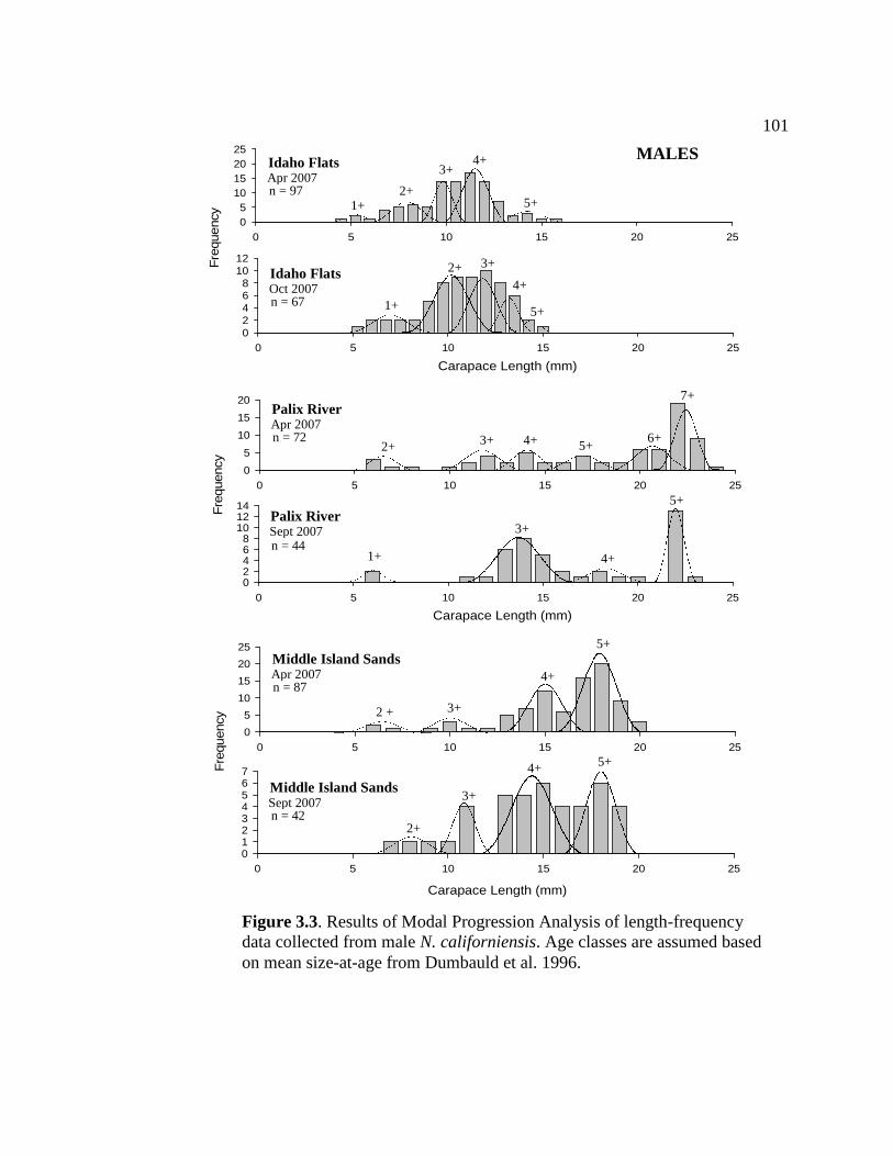
101

0 5 10 15 20 25

Fre

quen

cy 05

10152025

Carapace Length (mm)

0 5 10 15 20 2502468

1012

0 5 10 15 20 250

5

10

15

20

Carapace Length (mm)

0 5 10 15 20 25

Fre

quen

cy

02468

101214

0 5 10 15 20 25

Fre

quen

cy

0

5

10

15

20

25

Carapace Length (mm)

0 5 10 15 20 2501234567

Palix River Sept 2007 n = 44

Palix River Apr 2007 n = 72

Idaho Flats Oct 2007 n = 67

Middle Island Sands Apr 2007 n = 87

Middle Island Sands Sept 2007 n = 42

Idaho Flats Apr 2007 n = 97

5+

4+ 3+

2+ 1+

1+

2+ 4+

3+

5+

2+ 3+ 5+ 6+

7+

4+

1+

5+

4+

3+

3+ 2 +

4+

5+

2+

5+

3+

4+

Males

Figure 3.3. Results of Modal Progression Analysis of length-frequency data collected from male N. californiensis. Age classes are assumed based on mean size-at-age from Dumbauld et al. 1996.

MALES

102

0 5 10 15 200

20

40

60

80

Carapace Length (mm)0 5 10 15 20

Fre

quen

cy

0102030405060

0 5 10 15 200

10

20

30

40

Carapace Length (mm)0 5 10 15 20

Fre

quen

cy

05

101520253035

0 5 10 15 200

10203040506070

Carapace Length (mm)0 5 10 15 20

Fre

quen

cy

0

10

20

30

40

50

60

Idaho Flats Apr 2007 n = 191

Idaho Flats Oct 2007 n = 164

Palix River Apr 2007 n = 109

Palix River Sept 2007 n = 100

Middle Island Sands Apr 2007 n = 161

Middle Island Sands Sept 2007 n = 164

2+

3+

4+

5+

2+ 1+

3+

4+

2+ 3+

4+

5+

2+

5+

4+

3+

3+

4+

5+

3+

4+

5+

FEMALES

Figure 3.4. Results of Modal Progression Analysis of length-frequency data collected from female N. californiensis. Age classes are assumed based on mean size-at-age from Dumbauld et al. 1996.

103

0.0 0.5 1.0 1.5 2.0 2.5 3.0 3.505

101520253035

LF Index (ng/ug)0.0 0.5 1.0 1.5 2.0 2.5 3.0 3.5

Fre

quen

cy

0369

121518

0.0 0.5 1.0 1.5 2.0 2.5 3.0 3.505

1015202530

LF Index (ng/ug)0.0 0.5 1.0 1.5 2.0 2.5 3.0 3.5

05

10152025

0.0 0.5 1.0 1.5 2.0 2.5 3.0 3.505

1015202530

LF Index (ng/ug)0.0 0.5 1.0 1.5 2.0 2.5 3.0 3.5

0

5

10

15

20

Fre

quen

cyF

requ

ency

YB-Idaho Flats Apr 2007

n = 147

Oct 2007 n = 162

WB-Middle Island Sands Apr 2007

n = 149

Oct 2007 n = 129

WB-Palix River Apr 2007

n = 152

Oct 2007 n = 135

2+ 3+

4+ 5+

6+

7+

2+

5+ 3+ 6+ 7+

4+

8+ 10+

2+

4+

3+

5+

6+

8+ 9+ 7+

6+ 3+

4+

5+

7+

1+

7+

6+

5+

4+

3+

8+

9+ 10+

11+ 13+

2+

5+ 4+

3+ 6+

10+

7+ 8+

Figure 3.5. Results of MPA of LF index data from spring and fall 2007. Age classes are calibrated based on average LF index from the “reference age class” determined in the growth study from Chapter 2.

104

Estimated Age (yrs)0 2 4 6 8 10 12

LF IN

DE

X (

ng/u

g)

0.0

0.5

1.0

1.5

2.0

2.5

3.0

PR

MIS

YB

Figure 3.6. Regression of mean LF index against LF-estimated age for all three sites assessed. Age values are based on MPA of survey data collected in April 2007. Error bars represent the standard deviation from the mean LF index. Regression slopes were not significantly different from each other (n = 22, d.f. =2, adj R2 = 0.98, p<0.001, Z = NS)

105

Figure 3.7. Multiple linear regression of pooled LF index-at-age data from the spring and fall sample periods assuming equal slopes. An average increase in LF index of 0.20 ng µg-1 was exhibited between April and September. n = 867, d.f.= 1, R2 = 0.95, p <0.001.

SpringFall

LF estimated age (yrs)

LF In

dex

(ng/

ug)

0 3 6 9 12 15

0

1

2

3

4

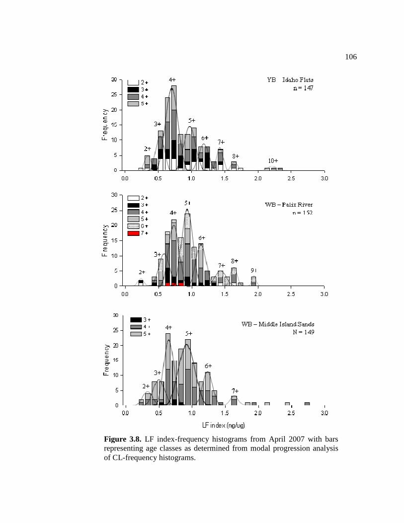
106

Figure 3.8. LF index-frequency histograms from April 2007 with bars representing age classes as determined from modal progression analysis of CL-frequency histograms.

107

LF index (ng µg-1) = 0.21* Age (yrs) – 0.056

Estimated Age (Years)

0 2 4 6 8 10 120.0

0.5

1.0

1.5

2.0

2.5

3.0

Age ModelPR MISYB

LF IN

DE

X (

ng/u

g)

Figure 3.9. LF-based age model for N. californiensis populations in Willapa Bay, Wash., and Yaquina Bay, Ore. Model was constructed from pooled LF data from the April survey collection. Solid line represents the LF accumulation model. The dashed line shows the 95% prediction interval for the model. R2 = 0.92, d.f. = 1, n = 443, p< 0.001.

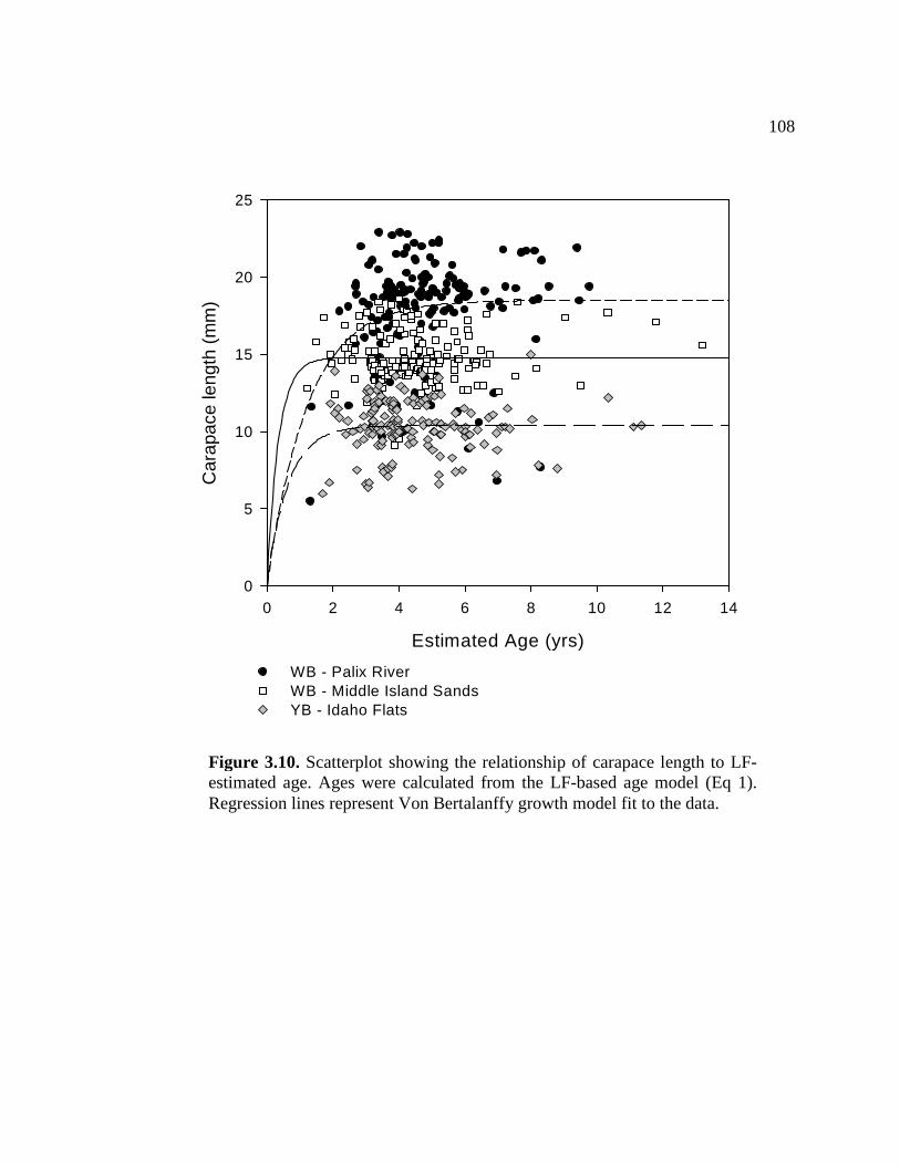
108

Figure 3.10. Scatterplot showing the relationship of carapace length to LF-estimated age. Ages were calculated from the LF-based age model (Eq 1). Regression lines represent Von Bertalanffy growth model fit to the data.

Estimated Age (yrs)

0 2 4 6 8 10 12 14

Car

apac

e le

ngth

(m

m)

0

5

10

15

20

25

WB - Palix RiverWB - Middle Island SandsYB - Idaho Flats

109

Figure 3.11. Recruitment history of N. californiensis in Willapa Bay, Wash., and Yaquina Bay, Ore. (Top) Long-term recruitment history for Palix River in Willapa Bay. Data range from 1989 to 2007. No recruitment data were collected from 1990 – 1992. (Bottom) Recruitment history at three study sites from 2004 – 2007. No recruits were found at the MIS study site during the years surveyed.

Year1990 1995 2000 2005

Rec

ruit

Den

sity

(sh

rimp

m-2

)

0

20

40

60

80

100

120

140

160

180

WB - Palix River

Year2004 2005 2006 2007

Rec

ruit

Den

sity

(sh

rimp

m-2

)

0

2

4

6

8

10

12

14

WB - Palix River YB - Idaho Flats

0 0 0

n/dn/d

110

Figure 3.12. Change in shrimp density at the three study locations over time. Density information is from annual surveys of the ghost shrimp population at each site. Data from the Palix River site in Willapa Bay extends from 1988 to 2007. Data from Middle Island Sands and Idaho Flats extend from 2005 and 2004 respectively.

Year1990 1995 2000 2005

Den

sity

(S

hrim

p m

-2)

0

100

200

300

400

500

600

WB - Palix RiverWB - Middle Island SandsYB - Idaho Flats

111

FEMALE April

Est. Age Class Mean Size SD Population SI 2 + 6.25 0.50 4 n.a 3 + 11.50 1.40 10 5.53 4 + 17.66 1.24 28 4.67 5 + 19.48 0.62 67 1.96*

September Est. Age Class Mean Size SD Population SI

2 + 10.02 1.03 4 n.a 3 + 14.34 0.86 12 4.57 4 + 18.66 1.09 50 4.43 5 + 19.86 0.05 33 1.51* 6 + 21.73 0.50 1 3.74

MALE April

Est. Age Class Mean Size SD Population SI 2 + 6.60 0.08 5 n.a. 3 + 11.83 1.00 9 5.81 4 + 14.23 0.51 7 3.18 5 + 16.87 0.75 7 4.19 6 + 20.95 1.42 22 3.76 7 + 22.29 0.54 22 1.37*

September Est. Age Class Mean Size SD Population SI

1 + 6.00 0.50 2 n.a. 3 + 13.96 1.22 23 9.24 4 + 18.41 1.09 5 3.86 5 + 22.07 0.50 14 4.60

Table 3.1. Palix River age structure as determined by MPA of length-frequency data. S I= separation index; * = not significant

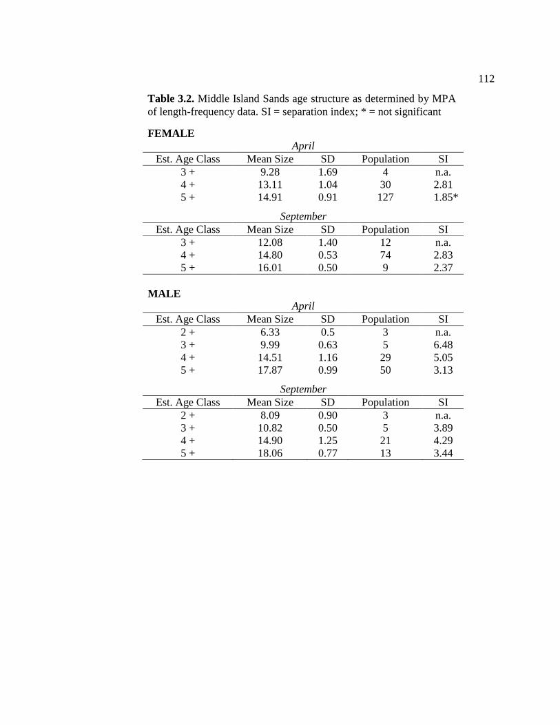
112

FEMALE April

Est. Age Class Mean Size SD Population SI 3 + 9.28 1.69 4 n.a. 4 + 13.11 1.04 30 2.81 5 + 14.91 0.91 127 1.85*

September Est. Age Class Mean Size SD Population SI

3 + 12.08 1.40 12 n.a. 4 + 14.80 0.53 74 2.83 5 + 16.01 0.50 9 2.37

MALE

April Est. Age Class Mean Size SD Population SI

2 + 6.33 0.5 3 n.a. 3 + 9.99 0.63 5 6.48 4 + 14.51 1.16 29 5.05 5 + 17.87 0.99 50 3.13

September Est. Age Class Mean Size SD Population SI

2 + 8.09 0.90 3 n.a. 3 + 10.82 0.50 5 3.89 4 + 14.90 1.25 21 4.29 5 + 18.06 0.77 13 3.44

Table 3.2. Middle Island Sands age structure as determined by MPA of length-frequency data. SI = separation index; * = not significant

113

FEMALE

April Est. Age Class Mean Size SD Population SI

2 + 7.54 0.87 18 n.a. 3 + 9.61 0.38 40 3.31 4 + 10.53 0.38 86 2.42 5 + 11.85 0.75 47 2.34

October Est. Age Class Mean Size SD Population SI

1 + 5.13 0.68 6 n.a. 2 + 9.82 1.12 17 5.21 3 + 10.91 0.77 132 1.15* 4 + 12.94 0.40 9 3.47

MALE

April Est. Age Class Mean Size SD Population SI

1 + 5.01 0.39 3 n.a. 2 + 7.83 1.00 20 4.06 3 + 9.78 0.38 11 2.83 4 + 11.35 0.97 57 2.33 5 + 14.48 0.78 6 3.58

October Est. Age Class Mean Size SD Population SI

1 + 6.50 0.83 7 n.a 2 + 10.30 1.17 35 3.78 3 + 12.30 0.69 18 2.15 4 + 13.48 0.38 5 2.21 5 + 14.54 0.40 2 2.70

Table 3.3. Idaho Flats age structure as determined by MPA of length-frequency data. SI = separation index; * = not significant

114

PALIX RIVER April

Est. Age Class Mean LF index SD Population SI 2 + 0.30 0.05 2 n.a. 3 + 0.68 0.10 31 5.15 4 + 0.83 0.09 44 1.70* 5 + 0.99 0.05 26 2.54 6 + 1.17 0.08 29 2.67 7 + 1.50 0.09 12 3.71 8 + 1.71 0.05 7 3.00 9 + 2.00 0.05 3 5.88

Χ2 = 4.0 df = 6 p = 0.68

September Est. Age Class Mean LF index SD Population SI

2 + 0.50 0.05 2 n.a. 3 + 0.76 0.05 10 5.07 4 + 0.97 0.69 34 3.27 5 + 1.19 0.09 37 2.88 6 + 1.46 0.08 22 3.27 7 + 1.72 0.12 17 2.56 8 + 2.00 0.11 11 2.44 10 + 2.60 0.05 1 7.94

Χ2 = 5.6 df = 6 p = 0.47

Table 3.4. Palix River age structure as determined by MPA of LF index-frequency data. SI = separation index; * = not significant.

115

MIDDLE ISLAND SANDS April

Est.Age Class Mean LF index SD Population SI 2 + 0.37 0.05 5 n.a 3 + 0.53 0.06 14 2.90 4 + 0.70 0.05 26 3.01 5 + 0.97 0.14 78 2.75 6 + 1.32 0.07 18 3.33 7 + 1.61 0.07 4 4.26

Χ2 = 2.13 df = 5 p = 0.83

September Est. Age Class Mean LF index SD Population SI

3 + 0.68 0.05 10 n.a. 4 + 0.91 0.10 28 3.07 5 + 1.21 0.11 29 2.93 6 + 1.48 0.06 20 3.24 7 + 1.76 0.09 11 3.74

Χ2 = 1.88 df = 4 p = 0.76

Table 3.5. Middle Island Sands age structure as determined by MPA of LF index-frequency data. SI = separation index.

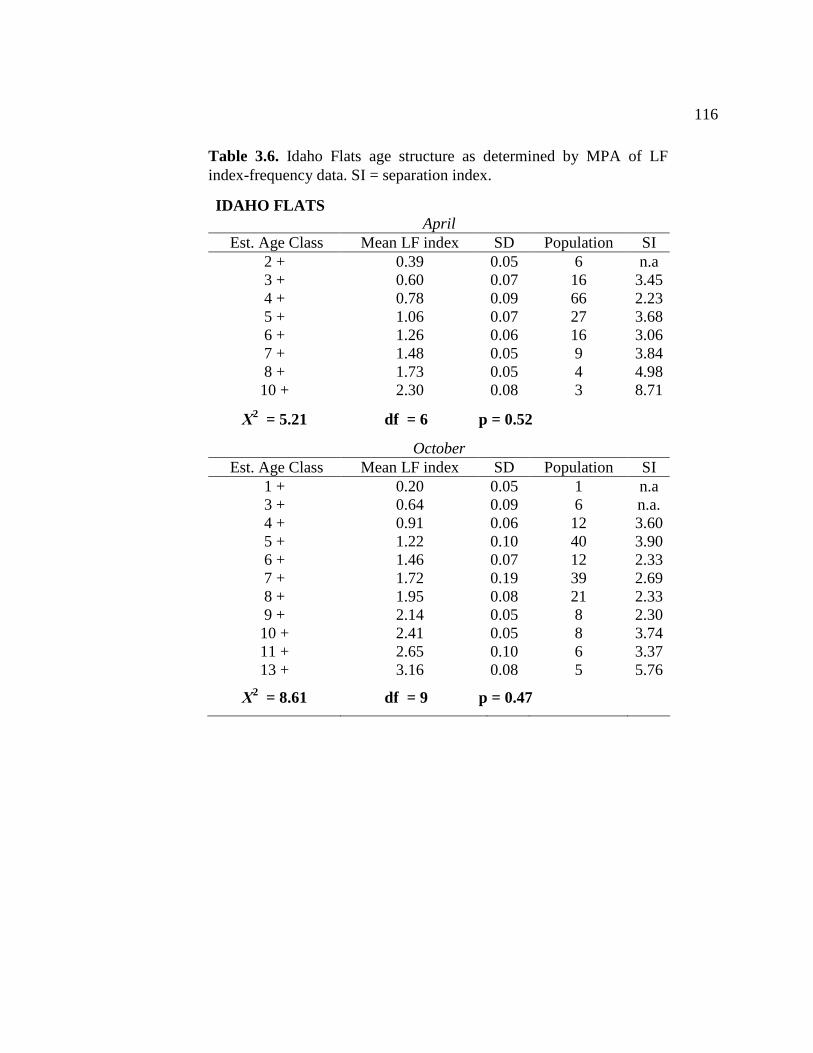
116

IDAHO FLATS April

Est. Age Class Mean LF index SD Population SI 2 + 0.39 0.05 6 n.a 3 + 0.60 0.07 16 3.45 4 + 0.78 0.09 66 2.23 5 + 1.06 0.07 27 3.68 6 + 1.26 0.06 16 3.06 7 + 1.48 0.05 9 3.84 8 + 1.73 0.05 4 4.98 10 + 2.30 0.08 3 8.71

Χ2 = 5.21 df = 6 p = 0.52

October Est. Age Class Mean LF index SD Population SI

1 + 0.20 0.05 1 n.a 3 + 0.64 0.09 6 n.a. 4 + 0.91 0.06 12 3.60 5 + 1.22 0.10 40 3.90 6 + 1.46 0.07 12 2.33 7 + 1.72 0.19 39 2.69 8 + 1.95 0.08 21 2.33 9 + 2.14 0.05 8 2.30 10 + 2.41 0.05 8 3.74 11 + 2.65 0.10 6 3.37 13 + 3.16 0.08 5 5.76

Χ2 = 8.61 df = 9 p = 0.47

Table 3.6. Idaho Flats age structure as determined by MPA of LF index-frequency data. SI = separation index.

117

PALIX RIVER Est. Age Class April Est. Age Class September ∆ LF

2 + 0.30 2 + 0.50 0.20 3 + 0.67 3 + 0.76 0.09 4 + 0.83 4 + 0.97 0.14 5 + 0.99 5 + 1.19 0.20 6 + 1.17 6 + 1.46 0.29 7 + 1.50 7 + 1.72 0.22 8 + 1.71 8 + 2.00 0.29 9 + 2.00 - - - - - 10 + 2.60 -

Average ∆ LF 0.20 SD 0.07

MIDDLE ISLAND SANDS Est. Age Class April Est. Age Class September ∆ LF

2 + 0.36 - - - 3 + 0.53 3 + 0.68 0.15 4 + 0.70 4 + 0.91 0.21 5 + 0.97 5 + 1.21 0.24 6 + 1.31 6 + 1.48 0.17 7 + 1.61 7 + 1.76 0.15

Average ∆ LF 0.18 SD 0.04

IDAHO FLATS Est. Age Class April Est. Age Class October ∆ LF

- - 1 + - - 2 + 0.39 - - - 3 + 0.60 3 + 0.64 0.04 4 + 0.78 4 + 0.91 0.13 5 + 1.06 5 + 1.22 0.16 6 + 1.26 6 + 1.46 0.20 7 + 1.48 7 + 1.72 0.24 8 + 1.73 8 + 1.95 0.22 - - 9 + 2.14 -

10 + 2.30 10 + 2.41 0.11 - - 11 + 2.65 - - - 13 + 3.16 -

Average ∆ LF 0.16 SD 0.07

Table 3.7. Table showing increase in average LF concentration for each age class between spring and fall 2007.

118

Variable Estimate Standard Error t-stat P

SPRING Constant -0.163 0.045 -3.62 0.002

AGE 0.236 0.006 41.11 < 0.001 SITE 0.011 0.015 0.07 0.463

Z NS

SE of Estimate = 0.061 R2 = 0.99 d.f. = 2 p = < 0.001

Variable Estimate Standard Error t-stat P FALL

Constant 0.018 0.025 0.75 0.463 AGE 0.250 0.003 89.78 < 0.001 SITE -0.034 0.009 -3.61 0.002

Z NS

SE of Estimate = 0.039 R2 = 0.99 d.f. = 2 p = < 0.001

Table 3.8. Results of multiple linear regression of mean LF index and site against LF-estimated age. Z = comparison of regression lines, NS; p> 0.05.

119

Site Slope ± SE Intercept ± SE r2 P n

Palix River Male 0.37 ± 0.34 16.56 ± 1.67 0.021 0.27 58 Female 0.34 ± 0.20 15.81 ± 0.99 0.032 0.08 94

Z NS Middle Island Sands Male -0.02 ± 0.13 16.12 ± 0.72 0.006 0.87 49 Female -0.06 ± 0.08 14.42 ± 0.37 0.050 0.50 100 Z NS Idaho Flats Male -0.13 ± 0.19 11.14 ± 0.95 0.100 0.52 45 Female 0.02 ± 0.09 10.15 ± 0.43 0.004 0.85 102 Z NS

Site L∞ (mm) K r2 P

Palix River 18.5 0.81 0.10 0.002 Middle Island Sands 14.8 2.88 0.01 0.670

Idaho Flats 10.4 1.57 0.01 0.320

Table 3.9. Results of multiple linear regression of size to LF-estimated age for both sexes. Z = comparison of regression slopes. NS; p>0.05.

Table 3.10. Parameter estimation for the Von Bertalanffy growth function (Eq.2) modeled by size-at-age for each survey site. L∞ = asymptotic length (mm); K = annual growth coefficient (yr-1). The parameter to was constrained to equal zero.

120 Chapter 4: Summary and Future Directions

The work presented in this study demonstrates the feasibility and practicality

of using the biochemical methods of LF quantification developed by Ju et al. (1999) to

assess age in the ghost shrimp, Neotrypaea californiensis. The difficulty in obtaining

accurate estimates of age in crustaceans has led researchers to explore alternative

techniques for age determination. Quantification of the autofluorescent age pigment,

lipofuscin (LF), has proven effective in accurately determining age in a number of

crustaceans, providing insight into population dynamics and factors controlling

growth. The development of effective management strategies for controlling the ghost

shrimp, N. californiensis, requires understanding of basic ecological processes

including recruitment, growth, longevity and mortality of natural populations.

Previously, these age-related processes were modeled for N. californiensis using body

length measurements as a surrogate for age. Because growth in crustaceans tends to be

highly variable and influenced by environmental factors, using size as a proxy for age

introduces significant sources of error in the development of population models.

In this study, LF was identified in the brain tissue of the ghost shrimp and a

method for LF quantification was established by optimizing currently applied

techniques. A growth calibration experiment was conducted to verify the technique

and showed that LF accumulation was correlated with time and not carapace length,

confirming the hypothesis that analysis of extractable LF is a better and more accurate

measure of age than body size. In addition, the calibration experiment showed that

growth rate varies spatially and is likely influenced by local environmental factors

121 such as food availability and population density. Temperature appeared to have little

effect on LF accumulation rate and this may be because ghost shrimp are highly

tolerant of extreme changes in temperatures during tidal cycles. However, the duration

of the study was only ten months and represents only one season and one year of

growth and LF accumulation. Long-term investigations of growth and LF

accumulation need to be conducted to identify factors influencing LF accumulation

rate and determine how LF accumulation varies on seasonal and interannual scales.

The biochemical techniques developed to determine age in N. californiensis

were used to assess age structure in three populations of ghost shrimp across two West

Coast estuaries. Age classes were calibrated with mean LF content from two year old

animals determined in the growth calibration study. Up to 13 year classes were found

in established adult populations. This estimate of maximum lifespan is significantly

longer than estimates of longevity previously reported in studies that have used

carapace length to determine age in N. californiensis. Young age classes were weak or

absent from all populations assessed which is not surprising considering the weak

recruitment that has been observed over the last five years.

A major outcome of this thesis was the construction of an LF-based age model

that can be used to predict age based on the protein-normalized LF content. Ages were

estimated for all animals sampled using the LF-based age model and comparison of

size-at-age showed growth rate to vary locally within populations and also among

populations across a larger spatial scale. The broad range of body sizes found within a

single age class proves that carapace length is an unreliable metric for comparison

among individuals from the same population or from separate populations. The single

122 age model produced in this study can be used to determine age in all three populations

assessed and therefore avoid problems inherent with comparisons based on body size.

The age model presented here is good to predict age only within a year of the actual

chronological age. Rearing studies should be conducted to complete the calibration for

LF accumulation in N. californiensis. This would reveal the fine scale variability in LF

accumulation and increase the precision of the age model.

Practical application of the LF aging technique to understand the demographic

structure of N. californiensis in West Coast estuaries has provided some clues into the

population biology of this organism. The results of this study clearly show that growth

rates are variable locally and across spatial scales. Potential sources of variability may

include food resource availability, tidal elevation, population density and social

hierarchy. Further studies investigating the direct influence of these factors are

recommended to gain a more in-depth understanding of how local conditions influence

growth. In addition, long-term investigations of how LF accumulates across broader

temporal and spatial scales are also needed confirm that a generic linear LF-based

model can be used to describe age in all populations or if separate models are needed

for different geographic regions.

This study did not compare the two commonly used methods of LF aging

(histological vs. biochemical). Because of the ongoing debate centered around the

reliability of these LF-based aging techniques, comparison of the two methods is

recommended to confirm that the biochemical techniques used in the current study

generate results similar to those produced with the more commonly used histological

123 method. This would establish age determination of N. californiensis using extractable

LF as reliable and eliminate some of the controversy associated with the method.

Overall, this study was successful in proving analysis of extractable LF as

more accurate method of age determination than body length measurements. The

results reported here are preliminary, however the evidence is compelling that

biochemical based aging can be widely used to assess age in N. californiensis and

facilitate more in-depth investigations of basic biological and ecological processes in

this species and could also be used for investigation of age and growth in other

thalassinid crustaceans.

LITERATURE CITED Ju, S-J., D.H. Secor and H.R. Harvey. 1999. Use of extractable lipofuscin for age determination of the blue crab, Callinectes sapidus. Marine Ecology Progress Series 185:171-179.

124 Bibliography Archer, P. E. 2008. Re-establishment of the native oyster, Ostrea conchaphila, in Netarts Bay, Oregon, USA. M.S. Thesis, Oregon State University, Corvallis, OR. Banas, N.S., B.M. Hicky, J.A. Newton and J.L. Ruesink. 2007. Tidal exchange, bivalve grazing, and patterns of primary production in Willapa Bay, Washington, USA. Marine Ecology Progress Series 341:123-139. Barki, A. and I. Karplus. 2004. Size rank and growth potential in redclaw crayfish (Cherax quadricarinatus): are stunted juveniles suitable for grow out? Aquaculture Research 35:559-567. Berkenbusch, K. and A. A. Rowden. 2003. Ecosystem engineering-moving away from 'just so'stories. New Zealand Journal of Ecology 27:67-73. Bhattacharya, C.G. 1967. A simple method of resolution of a distribution into Gaussian components. Biometrics 23:115-135. Belchier, M., P.M.J. Shelton and C.J. Chapman. 1994. The identification and measurement of fluorescent age-pigment in the brain of a crustacean (Nephrops norvegicus) by confocal microscopy. Comparative Biochemistry and Physiology B 108(2):157-164. Belchier, M., L. Edsman, M.R.J. Sheehy and P.M.J. Shelton. 1998. Estimating age and growth in long-lived temperate freshwater crayfish using lipofuscin. Freshwater Biology 39:439-446. Berman M.S., A.L. McVey and G. Ettershank. 1989. Age determination of Antarctic krill using fluorescence and image analysis of size. Polar Biology 9:267-271. Bird. E.M. 1982. Population dynamics of thalassinidean shrimps and community effects through sediment modification. PhD dissertation, University of Maryland, College Park, Maryland. Pp.140. Bluhm, B.A. and T. Brey. 2001. Age determination in the Antarctic shrimp Notocrangon antarcticus (Crustacea:Decapoda), using the autofluorescent pigment lipofuscin. Marine Biology 138:247-257. Bluhm, B.A., T. Brey and M. Klages. 2001. The autofluorescent age pigment lipofuscin: key to age, growth and productivity of the Antarctic amphipod Waldeckia obesa (Chevreux, 1905). Journal of Experimental Marine Biology and Ecology 258:215-235.

125 Bluhm, B., T. Brey, M. Klages and W.E. Arntz. 2001. Occurrence of the autofluorescent pigment, lipofuscin, in polar crustaceans and its potential as an age marker. Polar Biology 24:624-649.. Boulton, M., M. Rózanowska, B. Rózanowski and T. Wiess. 2004. The photoreactivity of ocular lipofuscin. Photochemical and Photobiological Sciences 3:759-764. Botsford, L.W., S.R. Wing, and J. L. Largier. 1998. Population dynamics and management implications of larval dispersal. South African journal of Marine Science 19:131 – 142. Brown, C.A., W.G. Nelson, B.L. Boese, T.H. DeWitt, P.M. Eldridge, J.E. Kaldy, H. Lee II, J. H. Power and D.R. Young. 2007. An approach to developing nutrient criteria for Pacific Northwest estuaries: A case study of Yaquina Estuary, Oregon. USEPA Office of Research and Development, National Health and Environmental Effects Laboratory, Western Ecology Division. EPA/600/R- 07/046. Pp.169. Brunk, U.T. 1989. On the origin of lipofuscin, the iron content of residual bodies, and the relation of these organelles to the lysosomal vacuome. A study on cultures human glial cells. Advances in Experimental Medicine and Biology 266:313- 320. Brunk, U.T. and A. Terman. 2002. Lipofuscin: Mechanisms of age-related accumulation and influence on cell function. Free Radical Biology and Medicine 33(5):611-619. Burt, WV and WB McAlister. 1959. Recent studies in the hydrography of Oregon Estuaries. Research briefs, Fish Commission of Oregon 7(1):14-27. Chapman, W.M. and G.D. Esveldt. 1943. The spawning and setting of the Pacific oyster (Ostrea gigas Thunberg). Biological Report 43A. Washington Department of Fisheries, Seattle. Pp. 41 Chew, K. K. 2002. Burrowing Shrimp verses Pacific Northwest Oysters. Aquaculture Magazine 28:71-75. Clarke, A., M.A. Kendall and D.J. Gore. 1990. The accumulation of fluorescent age pigments in the trochid gastropod Monodonta lineate. Journal of Experimental Marine Biology and Ecology 144:185-204. Corgos, A. P. Varisimo and J. Freire. 2006. Timing and seasonality of the terminal molt and mating migration in the spider crab, Maja brachdactyla: evidence of alternative mating strategies. Journal of Shellfish Research 25(2):577-587.

126 D’Abramo L.R., J.M. Heinen, H. R. Robinette and J.S. Collins. 1989. Production of the freshwater prawn Macrobrachium rosenbergii stocked as juveniles at different densities in temperature zone ponds. Journal of the World Aquaculture Society 20(2):81-89. DeWitt, T.H., K.F. Wellman, T. Wildman, D.A. Armstrong, and L. Bennett. 1997. An evaluation of the feasibility of using integrated pest management to control burrowing shrimp in the commercial oyster beds. Report Prepared for the Washington Department of Ecology by Batelle, Pacific Northwest Division, Richland, Washington. Pp. 256. DeWitt, T. W., A. F. D’Andrea, C. A. Brown, B. D. Griffen and P. M. Eldridge. 2004. Impact of burrowing shrimp populations on nitrogen cycling and water quality in western North American temperature estuaries. Pages 107-115 in Akio Tamaki, editor. Proceedings of the Symposium on Ecology of Large Bioturbators in Tidal Flats and Shallow Sublittoral Sediments – from Individual Behavior to their Role as Ecosystem Engineers, November 2003. Nagasaki University, Nagasaki, Japan. Dumbauld, B. R. 1994. Thalassinid shrimp ecology and the use of carbaryl to control populations on oyster ground in Washington estuaries. PhD dissertation, University of Washington, Seattle, Washington Pp. 192. Dumbauld, B.R., D.A. Armstrong and K.L. Feldman.1996. Life-history of two ympatric thalassinidean shrimps, Neotrypaea californeisis and Upogebia ugettensis, with implications for oyster culture. Journal of Crustacean Biology 6(4):689-708. Dumbauld, B.R., K.M. Brooks and M.H. Posey. 2001. Response of an estuarine benthic community to application of the pesticide carbaryl and cultivation of pacific oysters (Crassostrea gigas) in Willapa Bay, Washington. Marine Pollution Bulletin 42:826-844. Dumbauld, B.R., S. Booth, D. Cheney, A. Suhrbier and H. Beltran. 2006. An integrated pest management program for burrowing shrimp control in oyster aquaculture. Aquaculture 261: 976-992. Eldred, G.E., G.V. Miller, W. S. Stark and L.Feeney-Burns.1982. Lipofuscin: Resolution of discrepant fluorescence data. Science 216:757-759. Elleder M. in Age Pigments, R.S. Sohal, ed. (Elsevier/North-Holland Biomedical ress, Amsterdam, 1981). Pp.204-241.

127 Estes, P.S. 1986. Cardiovascular and respiratory responses of the ghost shrimp, Callianassa californiensis Dana, to the pesticide carbaryl and its hydrolytic product 1-napthol. M.S. Thesis, Oregon State University, Corvallis, Oregon. Ettershank, G., I. Macdonnell and R. Croft. 1983. The accumulation of age pigment by the fleshfly Sarcophaga bullata Parker (Diptera:Sarcophagidae) Australian Journal of Zoology 31:131-138. Feldman, K. L., D.A. Armstrong, B.R Dumbauld, T.H. Dewitt and D.C. Doty. 2000. Oysters, crabs, and burrowing shrimp: Review of an environmental conflict over aquatic resources and pesticide use in Washington State’s (USA) coastal estuaries. Estuaries 23(2):141-176. Folch, J., M. Lees and G.H.S Stanley. 1957. A simple method for the isolation and purification of total lipids from animal tissues. Journal of Biological Chemistry 226:497-509. Fonseca D.B., M.R.J. Sheehy and P.M.J. Shelton. 2003. Unilateral eyestalk ablation reduces neurolipofuscin accumulation rate in the contralateral eyestalk of a crustacean, Pacifastacus leniusculus. Journal of Experimental Marine Biology and Ecology 289: 277-286. Fonseca, D.B., C.L. Brancato, A.E. Prior, P.M.J. Shelton and M.R.J. Sheehy. 2005. Death rates reflect accumulating brain damage in arthropods. Proceedings of the Royal Society B 272:1941-1947. Fukuto, T.R.1990. Mechanism of action of Organophosphorous and carbamate insecticides. Environmental Health Perspectives. 87:245-254. Gayanilo, F.C., P. Sparre and D. Pauly. FAO-ICLARM Stock assessment tools II (FiSAT II). Revised Version. 2005. FAO, Rome, Italy. Griffis, R.B. and T.H.Suchanek. 1991. A model of burrowing architecture and trophic modes in thalassinidean shrimp (Decapoda: Thalassinidea). Marine Ecology Progress Series 79:171-183. Gu. Hainan, A.J. Anderson, P.B. Mather and M. F. Capra. 1996. Effects of feeding level and starvation on growth and water and protein content in juvenile redclaw crayfish, Charax quadricarinatus (von Martens). Marine and Freshwater Research 47: 745-728. Gulland, J.A. and A.A. Rosenberg. 1992. A review of length-based approaches to assessing fish stocks. FAO Fisheries Technical Paper 323. Rome, FAO. 100 pp.

128 Hannover, A. 1842. Mikroskopiske undersögelser af neresysteme. Kgl. Danbske Videsk. Kabernes Selkobs naturv. Math. Aft. Copenhagen 10:1-112. Hartnoll, R.G. 1982. Growth. In Bliss, D.E. and L.G. Abele (eds), The biology of Crustacea, 2, Embryology, Morphology and Genetics. Academic Press, New York. Pp 111-196. Hartnoll, R.G. 2001. Growth in Crustacea – twenty years on. Hydobiologia 449:111- 122. Harvey, H.R., D. H. Secor and S-J Ju. 2008. The use of extractable lipofuscin for age determination of crustaceans: reply to Sheehy (2008). Marine Ecology Progress Series 353: 307-311. Hasselblad, V. 1966. Estimation of parameters for a mixture of normal distributions. Technometrics 8(3):431-444. Hedgepeth, J. and S. Obrebski. 1981. Willapa Bay: A Historical Perspective and a Rationale for Research. Office of Biological Services, US Fish and Wildlife Service FWS/OBS-81/03. p.1-52. Hernandez-Llamas, A. and D.A. Ratkowsky. 2004. Growth of fishes, crustaceans and molluscs: estimation of the von Bertalanffy, Logistic, Gompertz and Richards curves and a new growth model. Marine Ecology Progress Series 282:237- 244. Hickey, B.M. 1989. Patterns and processes of circulation over the shelf and continental slope. Coastal Oceanography of Washington and Oregon, B.M. Hickey and M.R. Landry, Eds. Elsevier. Pp. 41-115. Hicky, B.M. and N.S. Banas. 2003. Oceanography of the U.S. Pacific Northwest coastal ocean and estuaries with application to coastal ecology. Estuaries 26:1010-1031. Hill, K.T. and C.T. Womersley. 1991. Critical aspects of fluorescent age – pigment methodologies: modification for accurate age assessment in aquatic organisms. Marine Biology 109:1-11. Hill, K.T. and C.T. Womersley. 1993. Interactive effects of some environmental and physiological variables on fluorescent age pigment accumulation in brain and heart tissues of an aquatic poikilotherm. Environmental Biology of Fishes 37(4):397-405. Hosack, G.R., B.R. Dumbauld, J.L. Ruesink and D.A. Armstrong. 2006. Habitat associations of estuarine species: comparisons of intertidal mudflat, seagrass

129 (Zostera marina) and oyster (Crassostrea gigas) habitats. Estuaries and Coasts 29: 1150-1160. Howe, R. L., A. P. Rees and S. Widdicombe. 2004. The impact of two species of bioturbating shrimp (Callianassa subterranea and Upogebia deltura) on sediment denitrification. Journal of the Marine Biological Association of the United Kingdom 84:629-632. Ingle, L., T.R. Wood and A.M. Banta. 1937. A study of the longevity, growth, reproduction and heart rate in Daphnia longspina as influenced by limitations on quantity of food. Journal of Experimental Zoology 76:325-352. Jolly, R.D., B.V. Douglas, P.M. Davey and J.E. Roiri.1995. Lipofuscin in bovine muscle and brain: a model for studying age pigment. Gerontology 41(supp 2):283-295. Ju, S-J., D.H. Secor and H.R. Harvey. 1999. Use of extractable lipofuscin for age determination of the blue crab, Callinectes sapidus. Marine Ecology Progress Series 185:171-179. Ju, S-J. 2000. Development and application of biochemical approaches to understanding age and growth in crustaceans. PhD thesis, University of Maryland, College Park, MD. Pp.139. Ju, S-J., D.H. Secor and H.R. Harvey. 2001. Growth rate variability and lipofuscin accumulation in the blue crab Callinectes sapidus. Marine Ecology Progress Series 224:197-205. Ju, S-J., D.H. Secor and H.R. Harvey. 2002. Demographic assessment of the blue crab (Callinectes sapidus) in Chesapeake Bay using extractable lipofuscins as an age markers. Fishery Bulletin 101:312-320. Karplus, I. and A. Barki. 2004. Social control of growth in the redclaw crayfish, Cherax quadricarinatus: testing the sensory modalities involved. Aquaculture 242:321-333. Katz, M.L. and W.G. Robinson Jr. 2002. What is lipofuscin? Defining characteristics and differentiation form other autofluorescent lysosomal bodies. Archives of Gerontology and Geriatrics 34:169-184. Keller, R. and H.-P. Orth. 1990. Hyperglygemic neuropeptided in crustaceans. In Scanes, C.G. and M.H. Stetson (eds), Progress in Comparative Endocrinology. John Wiley and Sons, New York: 265 – 271.

130 Klein Breteler, W.C. 1975. Laboratory experiments on the influence of environmental factors on the frequency of moulting and the increase in size at moulting of juvenile shore crabs, Carcinus maenas. Netherlands journal of Sea Research 9(1):100-120. Kodama, K., H. Shiraishi, M. Morita and T. Horiguchi. 2006. Verification of lipofuscin-based crustacean ageing: seasonality of lipofuscin accumulation in the stomatopod Oratosquilla oratoria in relation to water temperature. Marine Biology 150:131-140. Kogan, M. 1998. Integrated pest management: historical perspectives and contemporary developments. Annual Review of Entomology 43:243-270. Li, G., Y. Liao, X. Wang, S. Sheng and D. Yin. 2006. In situ estimation of the entire color and spectra of age pigment-like materials: application of a front surface 3D-fluorescence technique. Experimental Gerontology 41:328-336. Lutz, C.G. and W.R. Wolters.1986. The effect of five stocking densities on growth and yield of red swamp crayfish Procambarus clarkia. Journal of the World Aquaculture Society 17(1-4):33-36. MacGinite, G.E. 1934. The natural history of Callianassa californiensis Dana. American Midland Naturalist 15(2):166-177. MacGinitie, G.E. 1935. Ecological Aspects of a California Marine Estuary. American Midland Naturalist 16:629-765. Maggi, V. and P.N. Riddle. 1965. Histochemisty of tissue culture cells: a study of the effects of freezing and of some fixatives. Journal of Histochemisty and cytochemisty 13(5):310-317. Manning, R.B. and D.L. Felder. 1991. Revision of the American Callianassidae (Crustacea:Decapoda:Thalassinidea). Proceedings of the Biological Society of Washington 104:764-792. Mason, D. T. 1963. The growth response of Artimea salina (L.) to various feeding regimes. Crustaceana 5:138-150. Mauchline, J. 1977. Growth of shrimps, crabs and lobsters – an assessment. Journal du Consiel International pour l'Exploration de la Mer 37(2):162–169. Maxwell, KE. T.R. Matthews, M.R.J. Sheehy, R.D. Bertelsen and C.D. Derby. 2007. Neurolipofuscin is a measure of age in Panulirus argus, the Caribbean spiny lobster, in Florida. Biological Bulletin 213:55-66.

131 McCrow, L. T. 1972. The ghost shrimp, Callianassa californiensis Dana, 1854, in Yaquina Bay Oregon. M.S. Thesis, Oregon State University, Corvallis, Oregon. Pp 1-56. Medina, A., Y. Vila, C, Megina, I. Sobrino and F. Ramos. 2000. A histological study of the age-pigment, lipofuscin, in dendrobranchiate shrimp brains. Journal of Crustacean Biology 20(3):423-430. Mente, E. 2003. Nutrition, physiology, and metabolism of crustaceans. Science Publishers, Inc., Enfield, NH, USA. Pp.160. Mount, M.E. and F.W. Oehme. 1981. Carbaryl: a literature review. Residue Review 80:1-64. Mullin, M.M. and E.R. Brooks. 1988. Extractable lipofuscin in larval marine fish. Fishery Bulletin 86: 407-415. Murphy, M. L., S.W. Johnson and D.J. Csepp. 2000. A comparison of fish assemblages in eelgrass and adjacent subtidal habitats near Craig, Alaska. Alaska Fishery Research Bulletin 7: 11-21. Naranjo-Páramo, J., A. Hernandez-Llamas, and H. Villarreal. 2004. Effect of stocking density on growth, survival and yield of juvenile redclaw crayfish Cherax quadricarinatus (Decaposa: Parastacidae) in gravel-lined commercial nursery ponds. Aquaculture 242:197-206. Newall, R.C. 1969. Effect of fluctuations in temperature on the metabolism of intertidal invertebrates. American Zoologist 9:293-307. Newman, G.G. and D.E. Pollock. 1974. Growth of the rock lobster Jasus lalandii and its relationship to benthos. Marine Biology 24:339-346. Newton, J.A., E. Siegel, K. Nakata and B. Hickey. 2000. Controls on primary production in the Pacific coast estuary Willapa Bay: Oceanic and riverine forcing. Eos 80:253. Nicol, S. 1987. Some limitations on the use of the lipofuscin ageing technique. Marine Biology 93:609-614. O’Donovan, V. and O. Tully. 1996. Lipofuscin (age pigment) as an index of crustacean age: correlation with age, temperature and body size in cultured juvenile Homarus gammarus L. Journal of Experimental Marine Biology and Ecology 207:1-14.

132 Oh, C.-W. and R.G. Hartnoll. 2000. Effects of food supply on the growth and survival of the common shrimps, Crangon crangon (Linneaus, 1758)(Decapoda, Caridea). Crusteceana 73: 83-99. Olin, P.G. 2001. Current status of aquaculture in North America. In R.P. Subasinghe, P. Bueno, M.J. Phillips, C. Hough, S.E. McGladdery & J.R. Arthur, eds. Aquaculture in the Third Millennium. Technical Proceedings of the Conference on Aquaculture in the Third Millennium, Bangkok, Thailand, 20- 25 February 2000. pp. 377-396. NACA, Bangkok and FAO, Rome. Ouyang Y., J.E. Zheng and L.-T. Ou. 2006. Temporal and spatial distributions of sediment total organic carbon in an estuary river. Journal of Environmental Quality 35: 93-100. Parsons, D.G. and J. Fréchette. 1989. Fisheries for Northern Shrimp (Pandalus borealis) in the Northwest Atlantic from Greenland to the Gulf of Maine. In Marine Invertebrate Fisheries: Assessment and Management. J.F.Caddy (ed) Wiley-IEEE. p. 63-86. Paterson, B.D. and M.J. Thorne. 1995. Measurements of oxygen uptake, heart and gill bailer rates of the callianassid burrowing shrimp Trypaea australiensis Dana and its responses to low oxygen tension. Journal of Experimental Marine Biology and Ecology 194:39-52. Percy, K.L., D.A. Bella, C. Sutterlin and P.C. Klingeman. 1974. Descriptions and information sources for Oregon estuaries. Oregon Sea Grant Program, Oregon State University, Corvallis, OR. Pp. 294 Porta, E.A. 1991. Advances in age pigment research. Archives of gerontology and geriatrics 12:303-320. Porta, E.A. 2002. Pigments and aging: an overview. Annals of the New York Academy of Sciences 959:57-65. Posey , M.H. 1986. Changes in a benthic community associated with dense beds of a burrowing deposit feeder, Callianassa californiensis. Marine Ecology Progress Series 31:15-22. Posey, M.H. 1987. Effects of lowered salinity on activity of the ghost shrimp Callianassa californiensis. Northwest Science 61(2):93-96. Powell R.R. 1974. The functional morphology of the foregut of the thalassinid crustaceans Callianassa californiensis and Upogebia pugettensis. University of California Publications in Zoology 102:1-41.

133 Prentø, P. 1997. The effects of freezing, storage, and thawing on cell compartment integrity and ultrastructure. Histochemisty and Cell Biology 108:543-547. Ra’anan Z. and D. Cohen. 1985. Ontogeny of social structure and population dynamic in the giant freshwater prawn, Macrobrachium rosenbergii (de Man). In: Wenner AM (ed) Crustacean Issues 3. Factors in adult growth. AA Balkma, Rotterdam. Pp. 277-311. Reusink, J.L., B.E. Feist, C.J. Harvey. J.S. Hong, A.C. Trimble and L.C. Wisehart. 2006. Changes in productivity associated with four introduced species:ecosystem transformation of a ‘pristine’ estuary. Marine Ecology Progress Series 311:203-215. Roegner, G.C. and A.L. Shanks. 2001. Import of coastally-derived chlorophyll a to South Slough, Oregon. Estuaries 24:224-256. Shanks A.L. and G.C. Roegner. 2007. Recruitment limitation in Dungeness crab populations is driven by variation in atmospheric forcing. Ecology 88(7):1726- 1737. Sheehy, M.R.J. 1989. Crustacean brain lipofuscin: an examination of the morphological pigment in the fresh-water crayfish Cherax cuspidatus (Parastacidae). Journal of Crustacean Biology 9(3):387-391. Sheehy, M.R.J. 1990. Widespread occurrence of fluorescent morphological lipofuscin in the crustacean brain. Journal of Crustacean Biology 10(4):613- 622. Sheehy, M.R.J. 1990. Potential of morphological lipofuscin age-pigment as an index of crustacean age. Marine Biology 107:439-442. Sheehy, M.R.J. 1996. Quantitative comparison of in situ lipofuscin concentration with soluble autofluorescence intensity in the crustacean brain. Experimental Gerontology 31:421-432. Sheehy, M.R.J. 2002a. A flow-cytometric method for quantification of neurolipofuscin and comparison with existing histological and biochemical approaches. Archives of Gerontology and Geriatrics 34:233-248. Sheehy, M.R.J. 2002b. Role of environmental temperature in aging and longevity: insights form neurolipofuscin. Archives of Gerontology and Geriatrics 34:287- 310.

134 Sheehy, M.R.J. and G. Ettershank.1988. Extractable age pigment-like autofluorescence and its relationships to growth and age in the water-flea Daphnia carnata King (Crustacea:cladocera). Australian journal of Zoology 36:611-625. Sheehy, M.R.J., J.G. Greenwood and D.R. Fielder. 1994. More accurate chronological age determination of crustaceans from field situations using the physiological age marker, lipofuscin. Marine Biology 121: 237-254. Sheehy, M.R.J., E. Cameron, G. Marsden and J. McGrath. 1995. Age structure of female giant tiger prawns Penaus monodon as indicated by neuronal lipofuscin concentration. Marine Ecology Progress Series 117:59-63. Sheehy, M.R.J., P.M.J. Shelton, J.F. Wickins, M. Belchier and E. Gaten. 1996. Ageing the European lobster Homarus gammarus by the lipofuscin in its eyestalk ganglia. Marine Ecology Progress Series 143: 99-111. Sheehy, M.R.J., N. Caputi, C. Chubb and M. Belchier. 1998. Use of lipofuscin for resolving cohorts of western rock lobster (Panulirus Cygnus).Canadian Journal of Fisheries and Aquatic Sciences 55:925-936. Sheehy M.R.J. and R.C.A. Bannister. 2002. Year-class detection reveals climatic modulation of settlement strength in the European lobster, Homarus gammarus. Canadian Journal of Fisheries and Aquatic Sciences 59:1132- 1143. Sheehy, M.R.J. and A.E. Prior. 2008. Progress on an old question for stock assessment of edible crab Cancer pagurus. Marine Ecology Progress Series 353:191-202. Sheehy, M.R.J. 2008. Questioning the use of biochemical extraction to measure lipofuscin for age determination of crabs: Comment of Ju et al. (1999, 2001). Marine Ecology Progress Series 353:303-306. Shirzad, F.F., S.P Orlando, C.J. Klein, S.E. Holliday, M.A. Warren and M.E. Monaco. 1988. Physical and Hydrological Characteristics, The Oregon Estuaries. National Estuarine Inventory: Supplement 1, NOAA. Smith,P.K., R. I. Krohn, G. T. Hermanson, A. K. Mallia, F. H. Gartner, M. D. Provenzano, E. K. Fujimoto, N. M. Goeke, B. J. Olson and D. C. Klenk. 1985. Measurement or protein using bicinchoninic acid. Analytical Biochemistry 150(1):76-85. Sohol, R.S. 1981. Relationship between metabolic rate, lipofuscin accumulation, and lysosomal enzyme activity during aging in the adult housefly, Musca domestica. Experimental Gerontology 16:347-355.

135 Sohol, 1981. Age Pigments. Biochemical Press, Elservier/ North Holland, Amsterdam. Sokal, R. R. and F. J. Rohlf. 1995. Biometry: the principles and practice of statistics in biological research. 3rd edition. W. H. Freeman and Co.: New York. 887 pp. Stevens, B.A. 1928. Callianassidae from the West Coast of North America. Publications Puget Sound Biological Station 6:315-369. Stevens, B.A. 1929. Ecological observations of the Callinassidae of Puget Sound. Ecology 10(4):339-405. Swinbanks D.D. and J.L Luternauer. 1987. Burrow distribution of thalassinidean shrimp on a Fraser Delta tidal flat, British Columbia. Journal of Paleontology 61(2):315-332. Swinbanks D.D. and J.W. Murray. 1981. Bisedimentological zonation of Boundary bay tidal flats, Fraser River Delta, British Columbia. Sedimentology 28:201- 237. Tamone, S.L., M.M. Adams and J.M. Dutton. 2005. Effect of eyestalk-ablation on circulating ecdysteroids in hemolymph of snow crabs, Chionecetec opilio: physiological evidence for a terminal molt. Integrative and Comparative Biology 45:166-171. Terman. A. and U.T. Brunk. 1998. Lipofuscin: mechanisms of formation and increase with age. APMIS 106:265-276. Thompson, R.K. and A.W. Pritchard. 1969. Respiratory adaptations of two burrowing crustaceans, Callianassa californiensis and Upogebia pugettensis (Decapoda, Thalassinidea) Biological Bulletin 136: 274-287. Torres J.J., D.L. Gluck and J.J. Childress. 1977. Activity and physiological significance of the pleopods in the respiration of Callianassa californiensis (Dana) (Crustacea: Thalassinidea). Biological Bulletin: 152: 134-146. Vernet, M., J.R. Hunter and R.D. Vetter. 1988. Accumulation of age pigments (lipofuscin) in two cold water fishes. Fishery Bulletin 86: 401-407. Vila, Y., A. Medina, C. Megina, F. Ramos and I. Sobrino. 2000. Quantification of the age-pigments lipofuscin in brains of known-age, pond-reared prawns Penaeus japonicus (Crustacea, Decapoda). Journal of Experimental Zoology 286:120- 130.

136 Wahle, R.A., O. Tully and V. O’Donovan. 1996. Lipofuscin as an indicator of age in crustaceans: analysis of the pigment in the American lobster Homarus americanus. Marine Ecology Progress Series 138:117-123. Washington Department of Fisheries. 1970. Ghost shrimp control experiments 1960- 1968. Washington Department of Fisheries Technical Report 1. Olympia, Washington. Pp. 62. Washington Department of Fisheries and Washington Department of Ecology. 1985. Use of the insecticide Sevin to control ghost shrimp and mud shrimp in oysterbeds of Willapa and Grays Harbor. Final Environmental Impact Statement. Olympia, Washington. Pp.88. Yin D. and U. T. Brunk. 1991. Microfluorometric and fluorometric lipofuscin spectral discrepancies: a concentration-dependant metachromatic effect? Mechanisms of Ageing and Development 59: 95-109. Yin, D. 1996. Biochemical basis of lipofuscin, ceroid, and age pigment-like fluorophores. Free Radical Biology and Medicine 21:871-888. Zhou, S., T. Shirley and G. Kruse. 1998. Feeding and growth of the red king crab Paralithodes camtschaticus under laboratory conditions. Journal of Crustacean Biology 18:337-345.

137

APPENDICES

138 Appendix A

This section contains supplementary information about the life history and

growth of N. californiensis.

Figure A1. Molt stage data for N. californiensis in Yaquina Bay, Ore. Data points represent the proportion of individuals sampled every two weeks from Octobter 2005 to September 2006 that were in the premolt or intermolt phase of the molt cycle. The majority of molting and growth occurs between April and November.

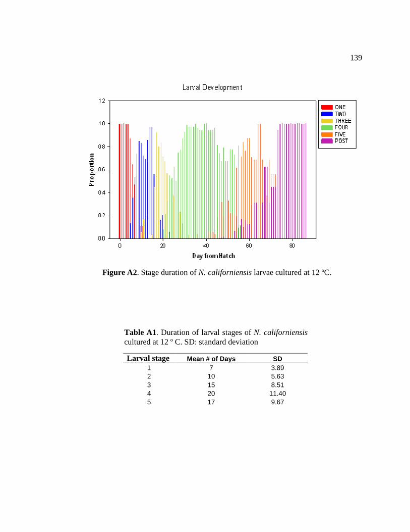
139

Larval stage Mean # of Days SD 1 7 3.89 2 10 5.63 3 15 8.51 4 20 11.40 5 17 9.67

Table A1. Duration of larval stages of N. californiensis cultured at 12 º C. SD: standard deviation

Figure A2. Stage duration of N. californiensis larvae cultured at 12 ºC.

140 Appendix B

Included in this appendix is data used to identify LF in N. californiensis and

optimize the method of age determination for the species.

Quinine Standard

Quinine Concentration (ng ml-1)

0 200 400 600 800 1000 1200 1400 1600

Flu

ores

cenc

e In

tens

ity (

LU)

0

200

400

600

800

1000

1200

Figure B1. Standard curve of quinine sulfate in 0.1N H2SO4 used to quantify LF concentration in brain tissue samples of N. californiensis. y = 0.6955(x); R2 = 0.9996.

141

Flu

ores

cenc

e In

tens

ity (

LU

)

Fluorescence Intensity (LU)

x464.610

0255075

100125

050

100

150200250

0 25 50 75 100 125

0 25 50 75 100125

x276.610

x451.520

0 50 100 150

0 50 100 150 200 250

x273.520

0

25

50

75

100125

0

50

100

150

x367.520

020406080100

0 20 40 60 80 100

464 / 615

281 / 615

450 / 515

367 / 515

273 / 515

Figure B2. Matrix of correlated fluorescence intensities from 5 Ex/Em maxima observed in N. californiensis. N = 51.

142

LF C

once

ntra

tion

(ng/

ug)

0

10

20

30

40

50

60

LF c

once

ntra

tion

(ng/

ug)

0

20

40

60

80

100

120

140

160

Fresh Frozen 2 weeks Frozen 6 months

LF A

LF B

a

bb

a

b b

Fresh Frozen 2 weeks Frozen 6 months

Figure B3. Comparison of LF concentration from shrimp processed frozen and those frozen two weeks and six months. Groups with the same letter (a,b) are not statistically different from each other

143 Appendix C

This section contains data from growth/calibration study (Chapter 2).

Sample Mean CL SD N Mean LF SD N Cal A 7.47 0.50 28 0.37 0.14 28

SWA 8.61 0.64 16 0.43 0.17 15 SWC 9.31 1.27 9 0.60 0.21 9 SWD 9.84 1.40 10 0.56 0.16 10

ILA 7.89 0.60 17 0.46 0.18 17 ILC 8.81 0.86 14 0.70 0.13 14 ILD 8.93 0.67 13 0.72 0.15 13

IHA 7.48 0.45 26 0.47 0.15 26 IHC 7.63 0.32 18 0.67 0.12 18 IHD 7.84 0.36 16 0.69 0.13 16

Table C1. Mean body size and LF data from each sample collected for the field growth/calibration experiment. CL: carapace length; SD: Standard deviation; N: sample size.

144

IFH IFL SWI Month Temp (ºC) SD Temp (ºC) SD Temp (ºC) SD

Jul-07 17.60 2.72 17.76 2.29 14.82 3.28 Aug-07 16.89 2.53 16.35 2.60 12.99 2.34 Sep-07 14.36 2.45 13.90 2.21 11.16 1.16 Oct-07 11.93 1.65 11.83 1.71 11.57 0.91 Nov-07 8.66 2.20 8.86 2.18 9.74 1.05 Dec-07 7.00 1.85 7.41 1.98 8.51 1.10 Jan-08 5.98 1.91 6.24 2.07 7.61 1.05 Feb-08 8.22 1.96 8.24 1.99 8.48 1.28 Mar-08 9.17 2.02 9.31 2.10 9.45 1.05 Apr-08 10.29 2.68 10.26 2.77 9.81 1.96

Table C2. Average monthly temperature from temperature probes placed 10 cm below the sediment surface at each study site in Yaquina Bay. IFH: Idaho Flats High; IFL: Idaho Flats Low; SWI: Seawall Island; SD: Standard deviation

145 Appendix D

This appendix contains more information about the outlier analysis conducted

to remove outliers from the data set that may have resulted from contamination during

processing N. californiensis brain tissue samples.

146

Figure D1. Scatterplot and linear regression showing relationship of LF concentration to carapace length in previously frozen N. californiensis with outliers removed. Note differences in x-axes scales

Carapace Length (mm)

6 8 10 12 14 16 18 20 22 24

LF c

onc

(ng

ml-1

)

0

20

40

60

80

100

120

140

160

Carapace Length (mm)

8 10 12 14 16 18 200

10

20

30

40

50

60

70

80

Carapace Length (mm)

4 6 8 10 12 14 16

0

10

20

30

40

50

LF c

onc

(ng

ml-1

)LF

con

c (n

g m

l-1)

Palix River

Middle Island Sands

Idaho Flats

147

PR

Sample # Sex CL (mm) LF conc. (ng ml-1)

Protein conc. (µg ml-1)

LF Index (ng µg-1)

5 m 21.0 165.205 398.088 0.415 6 m 21.4 192.164 586.976 0.327 7 m 21.6 490.046 127.021 3.858 9 f 5.7 20.417 28.110 0.726

10 f 18.6 82.459 155.176 0.531 14 f 19.2 93.386 187.532 0.498 39 m 5.2 13.803 10.916 1.264 56 f 5.7 35.370 51.051 0.693

231 m 16.7 91.445 175.571 0.521 237 m 6.0 57.944 35.042 1.654 273 m 5.5 25.162 16.091 1.564 283 m 10.6 18.404 6.903 2.666

MIS

Sample # Sex CL (mm) LF conc. (ng ml-1

Protein conc. (µg ml-1)

LF Index (ng µg-1)

153 m 17.9 43.853 71.131 0.617 154 m 18.7 54.349 115.256 0.472 163 m 19.1 49.173 76.506 0.643 175 m 18.5 140.043 237.048 0.591 193 f 9.8 33.357 21.247 1.570 495 m 9.0 22.717 13.199 1.721 574 m 6.7 18.260 14.923 1.224

YB

Sample # Sex CL (mm) LF conc. (ng ml-1

Protein conc. (µg ml-1)

LF Index (ng µg-1)

357 m 4.9 3.882 3.866 1.004 369 m 6.7 13.372 6.508 2.055 419 m 15.3 24.874 39.784 0.625 458 m 4.5 3.738 7.382 0.506

Table D1. Outlying data points from April survey that were removed from the analyses. These data points were removed because they had studentized residuals greater than absolute value 4 when carapace length was regressed against LF concentration or protein concentration. CL: carapace length.

148

PR

Sample # Sex CL (mm) LF conc. (ng ml-1)

Protein conc. (µg ml-1)

LF Index (ng µg-1)

755 m 14.7 42.991 12.438 3.457 782 m 11.9 39.396 14.563 2.705 809 f 8.5 26.168 11.192 2.338 816 m 5.1 15.528 10.026 1.549 862 f 19.5 120.201 170.029 0.707

MIS

Sample # Sex CL (mm) LF conc. (ng ml-1)

Protein conc. (µg ml-1)

LF Index (ng µg-1)

605 m 7.9 19.842 6.810 2.914 677 f 14.8 19.698 7.449 2.644 709 m 6.4 8.483 6.833 1.241 725 f 13.2 59.094 128.049 0.461 730 m 12.8 40.403 84.549 0.478

YB

Sample # Sex CL (mm) LF conc. (ng ml-1)

Protein conc. (µg ml-1)

LF Index (ng µg-1)

966 f 11.2 30.295 5.750 5.269 979 m 12.7 3.408 22.405 0.152

1016 m 5.8 15.516 5.830 2.662 1025 f 12.3 28.457 4.045 7.034 1053 f 11.1 6.746 15.375 0.439 1055 m 8.3 5.596 1.600 3.497 1056 f 5.4 3.583 1.213 2.955

Table D2. Outlying data points from September survey that were removed from the analyses. These data points were removed because they had studentized residuals greater than absolute value 4 when carapace length was regressed against LF concentration or protein concentration. CL: carapace length.

149

LF concentration (ng ml-1) Protein concentration (µg ml-1) Site coefficient p R2 coefficient p R2 n

PR 5.51 <0.001 0.45 4.10 <0.001 0.18 135 MIS 2.97 <0.001 0.18 2.58 <0.001 0.11 129 YB 2.64 <0.001 0.32 1.37 <0.001 0.18 165

Table D3. Results of simple linear regression analyses of LF concentration and protein concentration against carapace length for all three sites surveyed with outliers removed. Regression analyses were conducted to identify potential outliers that were a result of contamination during processing.