Cash Flow Simulation Tool for Wind Power Investments in Viet...

1

Up-Scaling of Wind Power in Vietnam

Cash Flow Simulation Tool for Wind Power Investments in Viet Nam

Handbook

2

Imprint

Published by the Deutsche Gesellschaft für Internationale Zusammenarbeit (GIZ) GmbH

Registered offices Bonn and Eschborn, Germany Energy Support Programme Unit 042A, 4th Floor, Coco Building,

14 Thuy Khue, Tay Ho District Hanoi, Vietnam T + 84 4 39 41 26 05 F + 84 4 39 41 26 06 [email protected]/viet-nam

As at February 2016

Photo credits Maik Scharfscheer Model design and text Dr. Dominik Dersch (Mr.), freelance consultant for GIZ, Matobis AG, Investment Service E [email protected] GIZ is responsible for the content of this publication.

On behalf of the German Federal Ministry for Economic Cooperation and Development (BMZ) Alternatively: German Federal Foreign Office

Contact Peter Cattelaens (Mr.) Support to the Up-Scaling of Wind Power Project Manager T + 84 4 3941 2605 (ext 108) E [email protected]

mailto:[email protected]

3

Table of Contents

Table of Contents ................................................................................................... 3

Abbreviations ........................................................................................................ 4

List of Tables .......................................................................................................... 5

List of Figures ......................................................................................................... 5

1. Summary ........................................................................................................ 7 1.1 Scope and limitation of the model ................................................................................... 7 1.2 System requirements ........................................................................................................ 7 1.3 Workbook structure and sheet protection ....................................................................... 7 1.4 User expertise and error handling .................................................................................... 8

2. Model Description ........................................................................................ 10 2.1 Sheet ‘Input’ ................................................................................................................... 10 2.2 Sheet ‘Overview Report’ ................................................................................................. 14 2.3 Sheet ‘Key Results Report’ .............................................................................................. 15 2.4 Sheet ‘Graphics’ .............................................................................................................. 17 2.5 Sheet ‘Cashflow’ ............................................................................................................. 19 2.6 Sheet ‘Debt Financing’ .................................................................................................... 20 2.7 Sheet ‘O&M Costs’ .......................................................................................................... 21

3. The Scenario Simulation Tool ........................................................................ 23 3.1 Cashflows ........................................................................................................................ 23 3.2 Debt Financing ................................................................................................................ 24 3.3 O&M Cost ....................................................................................................................... 24 3.4 Scenarios in general ........................................................................................................ 24

4. Implementation aspects of the model ........................................................... 26

4

Abbreviations CDM Clean Development Mechanism CO2 Carbon Dioxide Emission DSCR Debt Service Coverage Ratio EBIDA Earnings after tax and Before Interest payments, Depreciation and

Amortization EBIDTA Earnings Before Interest payments, Depreciation, Tax and Amortization EBIT Earnings after depreciation and amortization but Before Interest payments

and Tax EBIT Margin EBIT divided by revenues GIZ Deutsche Gesellschaft für Internationale Zusammenarbeit GmbH IRR Internal Rate of Return LCOE Levelized Cost of Electricity LLCR Loan Life Coverage Ratio NPV Net Present Value O&M Operations and Management P50 Scenario Annual energy production in kWh which will be exceeded with 50%

confidence P75 Scenario Annual energy production in kWh which will be exceeded with 75%

confidence P90 Scenario Annual energy production in kWh which will be exceeded with 90%

confidence PLCR Project Life Coverage Ratio PV Present Value ROE Return On Equity VEPF Vietnamese Environmental Protection Fund

5

List of Tables Table 1: Input Project .................................................................................................................................................................... 10 Table 2: Input Wind Park ............................................................................................................................................................ 11 Table 3: Input Investment Cost Components ..................................................................................................................... 11 Table 4: Input Energy Production of the Wind Park ....................................................................................................... 11 Table 5: Input Electricity Tariff ................................................................................................................................................ 12 Table 6: Input Operations and Maintenance Cost Components ................................................................................. 12 Table 7: Input Debt Financing and Benchmarking .......................................................................................................... 12 Table 8: Input FX Exchange Rates and Tax Rates ............................................................................................................. 13 Table 9: Tax Rates in each year for three different tax scenarios (excerpt till year 10). ................................ 13 Table 10: Static Model Variables .............................................................................................................................................. 13 Table 11: Sample ‘Overview Report’ ...................................................................................................................................... 14 Table 12: Section Project and Equity Measures of the ‘Key Results Report’ ........................................................ 15 Table 13: Section Debt Service of the ‘Key Results Report’ ......................................................................................... 16 Table 14: Section Payback Equity and Project Cost of the ‘Key Results Report’ ................................................ 16 Table 15: Section Accounting Figures in first Year and ROE of the ‘Key Results Report’ ............................... 16 Table 16: Logical groups and GroupName of name variables. ................................................................................... 26

List of Figures Figure 1: The seven sheets of the model workbook ........................................................................................................... 7 Figure 2: Error message which appears if protected cells are accessed ................................................................... 8 Figure 3: The color conventions of the input sheet (detail from sheet). ................................................................ 10 Figure 4: Top Figure on sheet ‘Graphics’ .............................................................................................................................. 17 Figure 5: Middle Figure on sheet ‘Graphics’........................................................................................................................ 18 Figure 6: Bottom Figure on sheet ‘Graphics’ ...................................................................................................................... 18 Figure 7: The input section for indexation of energy production and tariffs ....................................................... 19 Figure 8: Illustration of various scenarios (grey squares) of the ‘Cashflows’ sheet. ........................................ 23 Figure 9: The simulation tool of the ‘Debt Financing’ sheet ........................................................................................ 24 Figure 10: The simulation tool of the ‘O&M Costs’ sheet. ............................................................................................. 24 Figure 11: The names of model input parameter (detail). ........................................................................................... 26 Figure 12: The names of model output parameter. ......................................................................................................... 27

6

01 Summary

7

1. Summary Within the framework of the project Up-Scaling of Wind Power in Viet Nam, the Ministry of Industry and Trade (MOIT) and GIZ are jointly implementing numerous activities to increase the capacities of public and private sector stakeholders in the wind sector in Viet Nam.

As part of the Action Area 2: Capacity Development of the project, GIZ has developed a cashflow modeling tool that provides for a way of assessing a wind power project with all its technological and financing parameters. With the development of the tool, trainings have taken (and continue to) take place with Vietnamese wind power project developers and local banks interested in financing wind power in the country.

This document provides a functional description of the Excel Tool GIZ_WindModel_Vietnam.xlsx. It is referred to as ‘model’ in the following. It is strongly recommended to create a backup of the original model file before modifying model parameters or configurations.

1.1 Scope and limitation of the model

The model is for educational purposes and in some ways a simplified simulation tool for illustration only. It is for non-commercial use and must not be used as basis of investment decisions. Notwithstanding its simplicity, the structure and functionality of the model allow to illustrate relevant properties of cash flow modelling of wind power projects. It is a valuable illustrative tool to evaluate the impact of key project inputs on the financial performance.

1.2 System requirements

The system requirement for the model is Excel 2003, 2007, 2010 or higher. The Excel-Workbook does not deploy Excel Macros or Visual Basic code, for the sake of security and flexibility. It applies standard built-in Excel functions only.

1.3 Workbook structure and sheet protection

The Excel workbook consists of seven Excel sheets. The tabs of the Workbook are shown in the Figure below.

Figure 1: The seven sheets of the model workbook

The model differentiates three basic sheet types:

1. Input: The sheet ‘Input’ (blue tab color) 2. Output: The sheets ‘Overview Report’, ‘Key Results Report’ and ‘Graphics’ (orange tab color) 3. Calculation: The sheets ‘Cashflows’, ’Debt Financing’ and ‘O&M Cost’ (green tab color)

The structure and content of each sheet is described in Section Error! Reference source not found.. In addition to the above sheets there exist two additional hidden sheets that hold information on the graphics data (sheet ‘Graphics Data’) and information on the content of drop-down boxes deployed in the model (sheet ‘Definitions’). They do not require user input.

8

In order to avoid unintentional changes to the structure and content of the model each sheet is protected by a password. Excel-cells which require user input can be accessed. Any other cells are protected from user inputs. If the user attempts to modify a protected cell the following error message appears.

Figure 2: Error message which appears if protected cells are accessed

The password to unprotect the sheets may be obtained on request to GIZ.

1.4 User expertise and error handling

The use of this model requires basic knowledge in financial analysis, cash flow modelling and key financial indicators. Very basic knowledge of MS-Excel is required to operate the Excel-Workbook. Both areas are beyond the scope of this document. Unless explicitly described in this document there is no input validation or input correction by the model. Hence the error handling and input validation is in the responsibility of the user.

Bac Lieu Wind Farm – Nov 2015, photo: GIZ

9

02

Model Description

10

2. Model Description This section describes each of the Excel sheets. They are structured in the three different types: Input, Output and Calculation as introduced above.

2.1 Sheet ‘Input’

2.1.1 Color Conventions and sheet structure

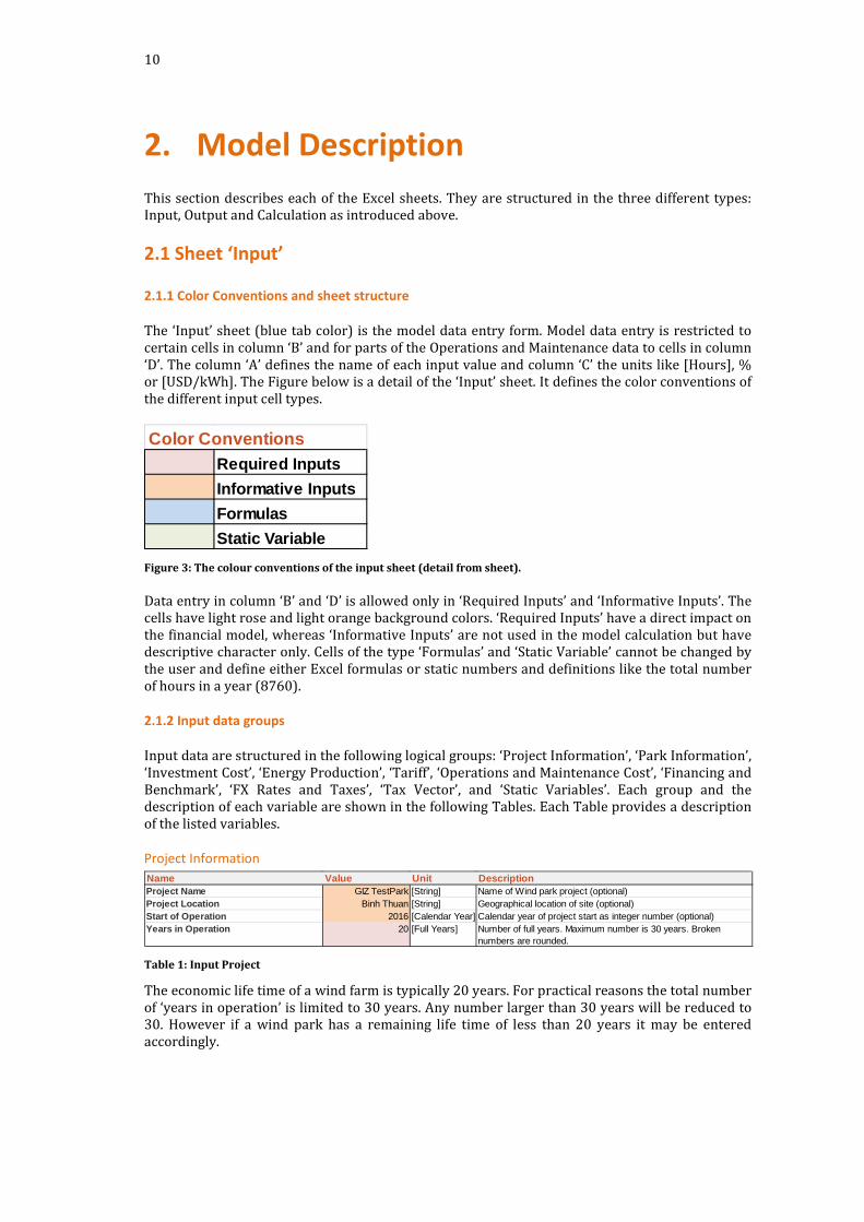
The ‘Input’ sheet (blue tab color) is the model data entry form. Model data entry is restricted to certain cells in column ‘B’ and for parts of the Operations and Maintenance data to cells in column ‘D’. The column ‘A’ defines the name of each input value and column ‘C’ the units like [Hours], % or [USD/kWh]. The Figure below is a detail of the ‘Input’ sheet. It defines the color conventions of the different input cell types.

Figure 3: The colour conventions of the input sheet (detail from sheet).

Data entry in column ‘B’ and ‘D’ is allowed only in ‘Required Inputs’ and ‘Informative Inputs’. The cells have light rose and light orange background colors. ‘Required Inputs’ have a direct impact on the financial model, whereas ‘Informative Inputs’ are not used in the model calculation but have descriptive character only. Cells of the type ‘Formulas’ and ‘Static Variable’ cannot be changed by the user and define either Excel formulas or static numbers and definitions like the total number of hours in a year (8760).

2.1.2 Input data groups

Input data are structured in the following logical groups: ‘Project Information’, ‘Park Information’, ‘Investment Cost’, ‘Energy Production’, ‘Tariff’, ‘Operations and Maintenance Cost’, ‘Financing and Benchmark’, ‘FX Rates and Taxes’, ‘Tax Vector’, and ‘Static Variables’. Each group and the description of each variable are shown in the following Tables. Each Table provides a description of the listed variables.

Project Information

Table 1: Input Project

The economic life time of a wind farm is typically 20 years. For practical reasons the total number of ‘years in operation’ is limited to 30 years. Any number larger than 30 years will be reduced to 30. However if a wind park has a remaining life time of less than 20 years it may be entered accordingly.

Color ConventionsRequired InputsInformative InputsFormulasStatic Variable

Name Value Unit DescriptionProject Name GIZ TestPark [String] Name of Wind park project (optional)Project Location Binh Thuan [String] Geographical location of site (optional)Start of Operation 2016 [Calendar Year] Calendar year of project start as integer number (optional)Years in Operation 20 [Full Years] Number of full years. Maximum number is 30 years. Broken

numbers are rounded.

11

Park Information

Table 2: Input Wind Park

The total installed capacity is a formula (blue field) it is the product of nominal output per turbine times number of turbines. Only the total installed capacity is used in due course but not the specific break-down in number and output of turbines.

Investment Cost

Table 3: Input Investment Cost Components

Investment cost may be broken down according to the above scheme. However the specific categories of investment cost are a suggestion only. They have no relevance to the model. Only the ‘Total Investment Cost’ (formula) is used in due course.

Note: In the current implementation the investment cost are not directly linked to the installed capacity. If e.g. the number of turbines are changed the investment cost have to be adjusted accordingly. However the investment cost components could be linked to the installed capacity (compare Table 2) by using an Excel formula.

Energy Production

Table 4: Input Energy Production of the Wind Park

The ‘Capacity Factor’ is a combined measure including effects like different loss types, the quality of park design, wind potential, scheduled maintenance and the power curve of the turbine. ‘Total Uncertainty’ is a combined statistical estimate of various uncertainties driven by losses, measurement and physical properties of wind. Both capacity factor and total uncertainty should be carefully assessed and are typically derived from bankable wind audits.

Name Value Unit DescriptionTurbine Manufacturer Wind AG [String] Name of turbine manufacturer (optional)Turbine Type XYZ [String] Name of turbine type (optional)Number of Turbines 15 [Integer] Total number of turbines installedNominal Output per Turbine 2,000 [kW] Nominal output per turbineHub Height 80 [Meter] Hub height of turbine nacelle in meter (optional)Rotor Diameter 90 [Meter] Rotor diameter in meter (optional)Installed Capacity 30,000 [kW] Installed capacity of wind farm (formula)

Name Value Unit DescriptionCivil Works 8,000,000 [USD] Cost component of investment cost in USDEquipment Cost 40,000,000 [USD] "Land Compensation 600,000 [USD] "Management Cost 400,000 [USD] "Consultant Cost 200,000 [USD] "Other Cost 7,800,000 [USD] "Total Investment Cost 57,000,000 [USD] Total investment cost in USD (formula, sum of components)Investment Cost per MW installed 1,900,000 [USD/MW] Relative investment cost per MW installed in USD (formula)Total Investment Cost local Currency 1,279,650,000,000 [VND] Total investment cost in VND (formula)

Name Value Unit DescriptionCapacity Factor (including all losses) 30% [%] Total net capacity factor including all losses and deductionsNet Output P50 p.a. 78,840,000 [kWh] Expected total net energy output of wind farm per year in kWhTotal Uncertainty 15% [%] Total uncertainty of expected energy output (estimate or provided

by wind audit)Net Output P75 p.a. 70,863,481 [kWh] Total net energy output of wind farm per year in kWh with 75%

probability of exceedanceNet Output P90 p.a. 63,684,390 [kWh] Total net energy output of wind farm per year in kWh with 90%

probability of exceedanceP50 full load hours 2,628 [Hours] Number of hours p.a. at full capacity to produce P50 energy yieldP75 full load hours 2,362 [Hours] Number of hours p.a. at full capacity to produce P75 energy yieldP90 full load hours 2,123 [Hours] Number of hours p.a. at full capacity to produce P90 energy yield

12

Tariff

Table 5: Input Electricity Tariff

Tariffs may consist of different components like credits from Clean Development Mechanism (CDM) or the Vietnamese Environmental Protection Fund (VEPF).

Operations and Maintenance Cost

Table 6: Input Operations and Maintenance Cost Components

The Operations and Maintenance Cost (O&M) may be broken down in different categories. In the Vietnamese context the ‘own electricity consumption’ is not determined separately but netted with the total electricity generation. Electricity consumption should be factored in the total capacity factor. Decommissioning cost is applied in the last year of operation. If a positive residual value of the wind farm is anticipated (scrap value, project rights, land value) decommissioning cost are entered as a negative value. The O&M cost may increase annually applying an indexation. Indexation is defined in column ‘D’ of the Input sheet.

Note: In the current implementation the O&M cost are not directly linked to the installed capacity. If e.g. the number of turbines is changed the O&M cost have to be adjusted accordingly. However the O&M cost components could be linked to the installed capacity (compare Table 2) by using an Excel formula.

Financing and Benchmark

Table 7: Input Debt Financing and Benchmarking

The model implements a single debt instrument only. Maturity may be entered in any number. However broken numbers are rounded to the closest year and the maximum maturity is restricted to 30 years. The loan is redeemed completely during the lending period. Two different redemption schemes are implemented: ‘linear’ or ‘annuity’. The selection of the redemption type is done via a drop-down box. Two benchmark rates must be provided to calculate the Levelized Cost of Electricity (LCOE), the Net Present Value (NPV) of the project (both by Target Project IRR) and the NPV of equity (Target Equity IRR).

Name Value Unit DescriptionTariff 0.104 [USD/kWh] Electricity tariff per kWh guaranteed for operational periodCDM Bonus 0.000 [USD/kWh] Carbon credit per kWh guaranteed for operational periodVEPF Bonus 0.000 [USD/kWh] Bonus from Vietnamese Environmental Protection Fund

guaranteed for operational periodTotal Tariff 0.104 [USD/kWh] Sum of all tariff components (formula)

Name Value Unit DescriptionMaintenance 714,000 [USD] Initial Maintenance cost p.a. in USDManagement 84,000 [USD] Initial Management cost p.a. in USDAdministrative Cost 52,500 [USD] Initial Administrative cost p.a. in USDInsurance Cost 61,000 [USD] Initial Insurance cost p.a. in USDBreakdown Insurance 44,000 [USD] Initial Breakdown Insurance cost p.a. in USDOwn Electricity Consumption - [USD] Initial Own Electricity Consumption cost p.a. in USDLand Lease - [USD] Initial Land Lease cost p.a. in USDProvisions 42,000 [USD] Initial Provisions p.a. in USDOther Cost 52,500 [USD] Initial Other Costs p.a. in USDTotal O&M Cost first year 1,050,000 [USD] Total initial operations and maintenance cost p.a. in USD (formula)Total O&M Cost per MW installed 35,000 [USD/MW] Total initial operations and maintenance cost p.a. and MW installed

in USD (formula)Total O&M Cost local FX first year 23,572,500,000 [VND] Total initial operations and maintenance cost p.a. and MW installed

in VND (formula)Decommissioning in last year - [USD] Decommissioning cost in last year of operations in USD. A

negative cost value defines a postive residual value.

Name Value Unit DescriptionMaturity of Loan 12 [Full Years] Maturity of loan in full years. Broken numbers are rounded.

Maximum value is 30 years. Interest Rate 2.00% [%] Interest rate in percentage to be paid annually Grace Period 1 [Full Years] Initial redemption free loan period in full yearsRedemption Type 1 [lin. =1, an. =2] Redemption type: Linear or Annuity Percentage Equity 30.00% [%] Percentage of total investment cost provided as equityTarget Project IRR & Discount Rate 10.00% [%] Target rate of return for project and used for LCOE calculationTarget Equity IRR 12.00% [%] Target rate of return for equity

13

FX Rates and Taxes

Table 8: Input FX Exchange Rates and Tax Rates

The exchange rate is used to convert investment, O&M cost and revenues into the local currency. The simulation of taxation is very basic. Regular corporate tax is assumed to be at a constant rate. Special tax breaks for renewable energy projects are implemented as follows. The length in full years and the respective tax levels of three different periods are defined, namely ‘First Period Tax Free’, ‘Second Period Reduced Tax’ and beyond. A taxation vector is automatically generated from the above parameter set. Three different taxation scenarios are implemented: ‘Full Flat Tax-Rate’ applying the regular corporate tax rate for each year, the ‘Discounted Tax-Rate’ which simulates the above described taxation rules for renewable energy projects and a ‘Tax Free Rate’ which applies a flat tax of the level ‘Tax Free Rate’.

Tax Vector

Table 9: Tax Rates in each year for three different tax scenarios (excerpt till year 10)

The three different taxation scenarios: ‘FullFlat’, ‘Discounted’, ‘Free’ may be selected in the scenario section of the ‘Cashflow’ sheet (please refer to Section Error! Reference source not found.).

Static variables are listed below. They are hard coded transformation and scaling factors. The static variables add transparency to the Excel formulas in the calculation and output sheets.

Static Variables

Table 10: Static Model Variables

Name Value Unit DescriptionFX-Rate 22,450 [VND/USD] Exchange rate for converting USD in VNDDepreciation Period (linear) 10 [Full Years] Period in full years to linearly write-off total investment costFlat Tax-Rate 20% [%] Regular corporate tax rateDiscounted Tax-Rate 10% [%] Reduced tax rate for renewable energy investmentsTax Free Rate 0% [%] Tax rate in first 'tax free' periodFirst Period Tax Free 4 [Full Years] Number of full years where 'tax free' period appliesSecond Period Reduced Tax 9 [Full Years] Number of full years after 'tax free' period where discounted tax

rate applies

Name Variable Name Values Values Values Values Values Values Values Values Values ValuesTax Year Year Vector 1 2 3 4 5 6 7 8 9 10Full Flat Tax-Rate FullFlat 20% 20% 20% 20% 20% 20% 20% 20% 20% 20%Discounted Tax-Rate Discounted 0% 0% 0% 0% 10% 10% 10% 10% 10% 10%Tax Free Rate Free 0% 0% 0% 0% 0% 0% 0% 0% 0% 0%

Name Value Unit DescriptionHours per Year 8760 [Hours] Number of hours in a regular year (365 days)MWh per KWh 0.001 [Number] Transformation factor to convert KWh to MWhCO2 Emission Factor of the Grid 0.6244 [tons/MWh] Emission factor of the vietnamese electricity grid in tons per MWhP75 Scaling Factor 0.674 [Number] Quantile measure of normal distribution which defines 75%

convidence level of exeedanceP90 Scaling Factor 1.282 [Number] Quantile measure of normal distribution which defines 90%



convidence level of exeedance

14

2.2 Sheet ‘Overview Report’

2.2.1 Purpose and Structure

The sheet ‘Overview Report’ (orange tab color) provides a user friendly summary report of model inputs. The report page is an output sheet only and neither requires nor allows user input. The layout of the ‘Overview Report’ fits to an A4 page and can be printed or saved to a pdf-file for documentary and audit purpose.

2.2.2 Content

The ‘Overview Report’ is structured in the following four groups: • Park Information • Key Production Figures (P50) • Key Cost Figures • Key Financing Figures

The sheet reflects the inputs provided by the user in the sheet ‘Inputs’ (compare Section 0 for description of variables). A sample ‘Overview Report’ is shown in the Table below:

Table 11: Sample ‘Overview Report’

GIZ TestPark

Project InformationProject Location Binh ThuanStart of Operation 2016Operational Period in Years 20 Number of Turbines 15 Turbine Type XYZNominal Output per Turbine [kW] 2,000 Installed Capacity [kW] 30,000 Hub Heigth in Meter 80.00 Rotor Diameter in Meter 90

Key Production Figures (P50)Net Output [MWh/a] 78,840 Capacity Factor 30.0%Full Load Hours 2,628 Total Tariff in [USDCent/kWh] 10.400 Total Revenues in USD in first Year 8,199,360 Total CO2 avoided [ton] first Year 49,228

Key Cost FiguresTotal Installation Cost in USD 57,000,000 Total Cost per MW Installed 1,900,000 Total Installation Cost in Mio. VND 1,279,650 Percentage Equity 30.0%Total Equity in USD 17,100,000 Total O&M Cost in USD in first Year 1,050,000

Key Financing FiguresTotal Debt in USD 39,900,000 Percentage Debt 70.0%Loan Period in Years 12 Grace Period in Years 1 Interest Rate 2.00%Redemption Type LinearTarget Project IRR (Discount Rate) 10.0%Target Equity IRR 12.0%

15

2.3 Sheet ‘Key Results Report’


The sheet ‘Key Results Report’ (orange tab color) is a user friendly summary report of key project and financial figures. All financial figures are calculated on the sheet ‘Cashflows’. The report page is an output and analysis sheet. The layout of the left-hand side of ‘Key Results Report’ (column A & B) fits to an A4 page and can be printed or saved to a pdf-file for documentary and audit purpose.

The grey shaded area on the right-hand side of the sheet (column D-N) is not write protected and allows user inputs. It is a dedicated area to log, compare and comment various model configurations. In the original release of the model the output of column ‘B’ is copied into column ‘D’. Any changes to the model input can easily be inspected. Formulas like ‘=D9-B9’ or ‘=D9=B9’ alert the user to differences.

2.3.2 Content

The ‘Key Results Report’ is structured in the following four groups: • Project and Equity Measures • Debt Service • Payback Equity and Project Cost • Accounting Figures in first Year and ROE

Each group and a description of the financial figures are shown in the following Tables. The table provides a description of the listed output variable of column ‘B’.

Table 12: Section Project and Equity Measures of the ‘Key Results Report’

Project and equity IRR are the most important key figures to assess the financial viability of a project. Equity IRR reveals the leverage effect using debt financing. The equity IRR will be larger than project IRR if loan interest rates are lower than pre-tax project IRR. The Net Present Value (NPV) quantifies the difference in value for a given target IRR. NPV will be positive if the pre-Tax IRR is larger than target IRR and vice versa.

Note: The IRR calculation relies on the built-in Excel function ‘IRR’. For large negative values of IRR Excel may not find a stable solution and delivers the error code ‘#NUM!. In that case the sum of cash flows over the life time of the project is much smaller than the up-front payment. Such a project could not be considered as financial viable.

Project and Equity Measures DescriptionProject IRR (Pre-Tax) 10.00% The internal rate of return of the unfunded project (100% equity)

before tax payments.Project IRR (Post-Tax) 8.78% The internal rate of return of the unfunded project (100% equity)

after tax.Target Project IRR 10.00% The user input of Target Project IRR for comparison purpose.NPV of Project (Pre-Tax) in USD 8,342 The Net Present Value (NPV) of the project. Future pre-Tax cash

flows are discounted with Target Project IRR.Equity IRR (Pre-Tax) 16.91% The internal rate of return of the invested equity before tax.Equity IRR (Post-Tax) 15.50% The internal rate of return of equity after tax.Target Equity IRR 12.00% The user input of Target Equity IRR for comparison purpose.NPV of Equity (Post-Tax) in USD 4,138,195 The Net Present Value (NPV) of equity. Future post-Tax cash

flows are discounted with Target Equity IRR.Loan Interest Rate 2.00% User input of loan interest rates for comparison purpose.LCOE (@ Target PIRR) in [USDcent/kWh] 11.44 Levelized Cost of Electricity (LCOE). All future O&M expenses

and the electricity productions are discounted with Target Project IRR. LCOE calculation does not involve any revenue, debt service or tax components.

16

The Levelized Cost of Electricity (LCOE) is a pre-tax figure parameterized by target project IRR. It is an important reference figure to compare different projects and explore if a given tariff would result in a financial viable project.

Table 13: Section Debt Service of the ‘Key Results Report’

Key figures for lenders are the Debt Service Coverage Ratio (DSCR), Loan and Project Life Coverage Ratio (LLCR and PLCR respectively). The definitions are given in the above Table.

The level of capital re-flow (equity and project) with respect to the initial capital invested is listed in the Table below.

Table 14: Section Payback Equity and Project Cost of the ‘Key Results Report’

Accounting figures are generally seen critical and of limited use assessing the financial viability of a project. However for the sake of completeness there are listed in the Results Report. They are printed in light grey color to flag its limited benefit.

Table 15: Section Accounting Figures in first Year and ROE of the ‘Key Results Report’

Debt Service DescriptionMinimum DSCR 1.30 Lowest value of Debt Service Coverage Ration (DSCR) observed

during loan period Average DSCR 1.68 Average value of DSCR during loan period Project Life Coverage Ratio (PLCR) @ Target PIRR 1.35 The present value of cash flows available for debt service divided

by the total debt. Future post-Tax cash flows are discounted with Target Project IRR.

Loan Life Coverage Ratio (LLCR) @ Target PIRR 1.13 The present value of cash flows available for debt service during loan period divided by the total debt. Future post-Tax cash flows are discounted with Target Project IRR.

Payback Equity and Project Cost DescriptionPayback % Equity after 5 Years 72% Percentage of equity repaid after 5 yearsPayback % Equity after 10 Years 139% Percentage of equity repaid after 10 yearsPayback % Equity after 20 Years 400% Percentage of equity repaid after 20 yearsPayback % Project Cost after 5 Years 58% Percentage of total investment cost repaid after 5 years for

unfunded projectPayback % Project Cost after 10 Years 115% Percentage of total investment cost repaid after 10 years for

unfunded projectPayback % Project Cost after 20 Years 206% Percentage of total investment cost repaid after 20 years for

unfunded project

Accounting Figures in first Year and ROE DescriptionEBIDTA 7,149,360 Earnings before interest payments, depreciation, amortization

and tax in the first year of operationEBIDA 7,149,360 Earnings after tax and before interest payments, depreciation,

amortization in the first year of operationEBIT 1,449,360 Earnings after depreciation and amortization but before

interest payments and tax in the first year of operationROE (Pre-Tax) 27.24% Total pre-tax distribution payments over project life-time

divided by invested equityROE (Post-Tax) 23.71% Total post-tax distribution payments over project life-time

divided by invested equity

17

2.4 Sheet ‘Graphics’


The output sheet ‘Graphics’ (orange tab color) is a visual illustration of the evolution of key cost and revenue components over time. The data behind the sheet ‘Graphics’ originates from the sheet ‘Cashflows’. However the data for the figures are linked from an additional sheet named ‘Graphics data’. This data sheet is hidden in the original shipment of the model.

The sheet ‘Graphics’ is an output sheet only. It neither requires nor allows input from the user. The layout of the figures fit to an A4 page and can be printed or saved to a pdf-file for documentary and audit purpose.

2.4.2 Content

The ‘Graphics’ sheet contains the following three Figures: • Cost Factors and Distribution Payments (top) • Debt Service (middle) • Distribution Payments (bottom)

Figure 4: Top Figure on sheet ‘Graphics’

The Figure ‘Cost Factors and Distribution Payments’ illustrates how the electricity revenues are broken down in the different components: distribution payments, taxes, O&M cost and debt service as function of the operations year.

18

Figure 5: Middle Figure on sheet ‘Graphics’

The Figure ‘Debt Service’ illustrates the three components interest rate payments, redemption (both left scale) and outstanding debt (right scale) as function of the operations year.

Figure 6: Bottom Figure on sheet ‘Graphics’

The Figure ‘Distribution Payments’ illustrates the level of the post-tax distribution payments to the equity investor in each year (left scale) and the cumulative payment relative to the invested equity (right scale).

19

2.5 Sheet ‘Cashflow’


The calculation sheet ‘Cashflow’ (green tab color) is the central calculation sheet of the model. It serves multiple purposes:

• The cash flow tables illustrate the evolution of all relevant components over the project life time

• Performs the calculation of tax and distribution payments for project and equity • Performs the calculation of key financial figures shown in the results report

The sheet is structured in three groups: • Header section with simulation tool • Main body section with detailed cash flow tables • Financial key figure section

2.5.2 Content The header group including the simulation tool is described in Section Error! Reference source not found. of this document.

A. Body section of sheet

The main body section is grouped in the different logical units:

i. Electricity Production & Revenues

This section holds the energy production, C02 avoidance, revenues from the different tariff components and the total revenues. Column ‘D’ lists the sum of each component over the operational period. The light rose cells in column ‘C’ hold an additional feature that allows indexation of energy production and tariffs. The input section is illustrated in the Figure below.

Figure 7: The input section for indexation of energy production and tariffs

A local indexation parameter could be applied to the electricity production caused by aging of different components like blade degradation, increasing electrical resistance of wiring or increasing friction of mechanical parts. In the example of the above Table a 1% annual decline (negative value) is applied. Similarly, an indexation of the various tariff components could be applied. In the above example the tariff increases by 4% each year. ii. Expenses

The expenses are linked from the ‘O&M Cost’ sheet and are described in Section 0 of this document. iii. Debt Service

The debt service is linked from the ‘Debt Financing’ sheet and is described in Section 0.

Electricity Production & Revenues Szenario Local Index ParameterEnergy production [kWh] 78,840,000 -1.00%CO2 avoidance [tons] 0.62440Tariff 0.1040 4.00%VEPF Bonus 0.0000 0.00%CDM Bonus 0.0000 0.00%

20

iv. Tax

The section on tax calculation lists the tax rate in each year, depreciation amount, the taxes paid in each year without debt financing and taxes paid in each year with debt financing.

v. Cash Flow and DSCR

This section calculates the accounting figures EBIDTA, EBIDA, EBIT, EBIT Margin (EBIT divided by revenues) and the free cash flow before and after tax in each year. The last line in this section shows the DSCR in each year and derives the average (column ‘C’) and minimum DSCR (column ‘D’). B. Key Figures Section

The section on financial key figures calculates the key figures listed in the ‘Key Results Report’. The key figures are described in Section 0.

Bac Lieu Wind Farm under construction – Nov 2015, photo: GIZ

21

2.6 Sheet ‘Debt Financing’


The calculation sheet ‘Debt Financing’ (green tab color) derives the cash flows of the debt service from the financing parameter. The header group including the simulation tool of this sheet is described in Section Error! Reference source not found. of this document.

2.6.2 Content

The debt service consists of the four components: • Outstanding debt at end of each year • Redemption amount in each year • Interest rate payments in each year • Total debt service in each year

The cash flow vectors of the debt service are linked to the ‘Debt Service’ section in the sheet ‘Cashflow’.

2.7 Sheet ‘O&M Costs’


The calculations sheet ‘O&M Costs’ (green tab color) derives the expenses for each cost component and for each year from the O&M Input parameter set (amount and indexation). The header group including the simulation tool of this sheet is described in Section Error! Reference source not found..

2.7.2 Content

The O&M cost components consist of the ten O&M categories: • Maintenance • Management • Administrative Cost • Insurance Cost • Breakdown Insurance • Own Electricity Consumption • Land Lease • Provisions • Decommissioning in last year (only single payment in last year of operation) • Other Cost

The cash flow vectors of the O&M cost components are linked to the ‘Expenses’ section in the sheet ‘Cashflow’.

22

03

The Scenario Simulation Tool

23

3. The Scenario Simulation Tool The scenario simulation tool allows assessing the impact of variations of the most relevant model parameter without modifying the original input settings. Scenario simulation functionality is located in the header section on the three calculation sheets: Cashflows, Debt Financing and O&M Costs. Although the calculation sheets are protected from modifications, the green cells below the column ‘Scaling Factors’ are an exception and allow user input.

Note: In order to alert the user to modifications, conditional formation provided by Excel changes the cell color from green to red if a scaling factor is different from ‘1’.

The functionality on each sheet is described in the following Sub Sections.

3.1 Cashflows

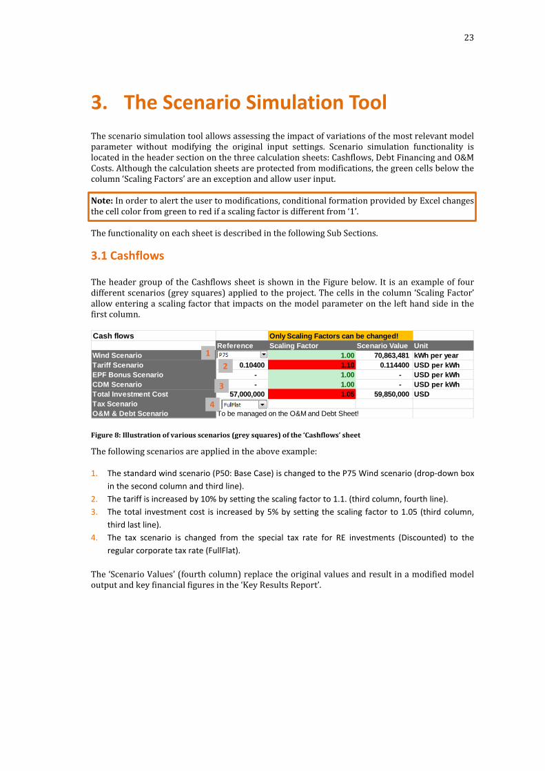
The header group of the Cashflows sheet is shown in the Figure below. It is an example of four different scenarios (grey squares) applied to the project. The cells in the column ‘Scaling Factor’ allow entering a scaling factor that impacts on the model parameter on the left hand side in the first column.

Figure 8: Illustration of various scenarios (grey squares) of the ‘Cashflows’ sheet

The following scenarios are applied in the above example:

1. The standard wind scenario (P50: Base Case) is changed to the P75 Wind scenario (drop-down box in the second column and third line).

2. The tariff is increased by 10% by setting the scaling factor to 1.1. (third column, fourth line). 3. The total investment cost is increased by 5% by setting the scaling factor to 1.05 (third column,

third last line). 4. The tax scenario is changed from the special tax rate for RE investments (Discounted) to the

regular corporate tax rate (FullFlat).

The ‘Scenario Values’ (fourth column) replace the original values and result in a modified model output and key financial figures in the ‘Key Results Report’.

Cash flows Only Scaling Factors can be changed!Reference Scaling Factor Scenario Value Unit

Wind Scenario 2 1.00 70,863,481 kWh per yearTariff Scenario 0.10400 1.10 0.114400 USD per kWhEPF Bonus Scenario - 1.00 - USD per kWhCDM Scenario - 1.00 - USD per kWhTotal Investment Cost 57,000,000 1.05 59,850,000 USDTax Scenario 1O&M & Debt Scenario To be managed on the O&M and Debt Sheet!

21

3

4

24

3.2 Debt Financing

Financing scenarios may be applied in the header section of the scenario simulation tool on the ‘Debt Financing’ sheet. The Figure below illustrates modified interest rates.

Figure 9: The simulation tool of the ‘Debt Financing’ sheet

In the above example the interest rates are doubled from 2% to 4% by applying a scaling factor of 2 (grey square, column 3, line 4). Scaling of ‘Maturity’ and ‘Grace Period’ is rounded to the next full year.

Note: Scaling of the debt amount (column 3, line 3) is done on the ‘Cashflows’ sheet via scaling of the total investment cost. The scaling factor on the ‘Debt Financing’ sheet is linked from there. Thus the cell is protected against modification on the ‘Debt Financing’ sheet. If cell protection is removed this link should be preserved. Otherwise inconsistent results may be observed by conflicting information on the two different sheets.

3.3 O&M Cost

Scenarios of the O&M cost are applied in the header section of the scenario simulation tool on the ‘O&M Costs’ sheet. O&M cost components are scaled by a unique factor which applies to all cost components. The Figure below illustrates a 10% decrease in O&M costs.

Figure 10: The simulation tool of the ‘O&M Costs’ sheet

3.4 Scenarios in general

Modifications of the model parameter which are not part of the scenario tool can be changed on the ‘Input’ Sheet. However, it is in the responsibility of the user to keep track of model adjustments.

Debt financing Only Scaling Factors can be changed!Parameter Scenario Value Scaling Factor ReferenceDebt amount 41,895,000 1.05 39,900,000 Interest rate 4% 2 2%Maturity 12 1 12Grace periode in years 1 1 1Redemption Linear LinearLinear redemption 3,808,636 Annuity repayment 4,782,274

1

O&M CostScaling Factor O&M Cost 0.90 Only Scaling Factor can be changed!

25

04 Implementation Aspects of the Model

26

4. Implementation aspects of the model The Excel programming makes usage of variable names. They are accessed in the Excel interface by selecting ‘Formulas>Name Manager’. The Figure below shows a subset of the variables defined in the model.

Figure 11: The names of model input parameter (detail)

The variable names follow a unique naming convention and consist of three name sections separated by a ‘dot’ e.g. Var.GroupName.VariableName. All variable names start with prefix ‘Var’ to distinguish them from other variables, the GroupName follows the logical groups introduced in Section 0 and are mapped as follows:

Table 16: Logical groups and GroupName of name variables

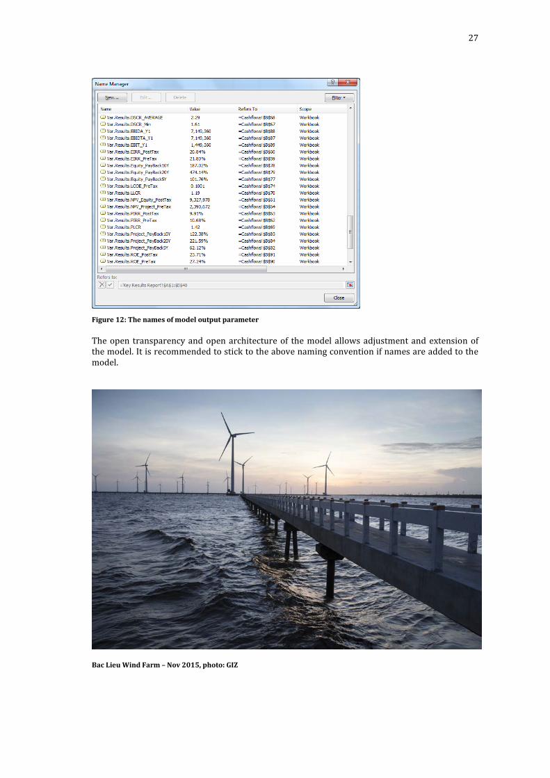
The key financial figures calculated on the ‘Cashflow’ sheet are also mapped onto variable names. They follow the naming convention: Var.Results.VariableName. All results variables are listed in the Figure below.

Logical Group GroupNameProject Information ProPark Information ParkInvestment Cost InvestEnergy Production ProdTariff TariffOperations and Maintenance Cost OMFinancing and Benchmark FinFX Rates and Taxes RatesTax Vector TaxStatic Variables FactorModel Key Figures Results

27

Figure 12: The names of model output parameter

The open transparency and open architecture of the model allows adjustment and extension of the model. It is recommended to stick to the above naming convention if names are added to the model.

Bac Lieu Wind Farm – Nov 2015, photo: GIZ

Cash Flow Simulation Tool for Wind Power Investments in Viet...

Documents

Transcript of Cash Flow Simulation Tool for Wind Power Investments in Viet...