CASH FLOW AND CAPITAL EMPLOYED: ITS RELATIONSHIP AND … · 2015-10-02 · 3 Abstract Titel: Cash...
59
GOTHENBURG UNIVERSITY SCHOOL OF BUSINESS, ECONOMICS AND LAW BACHELOR THESIS IN INDUSTRIAL AND FINANCIAL MANAGEMENT SPRING SEMESTER 2015 CASH FLOW AND CAPITAL EMPLOYED: ITS RELATIONSHIP AND IMPACT ON FIRM VALUE - A CASE STUDY OF A FIRM OPERATING IN THE TECHNIQUE DEVELOPMENT INDUSTRY AUTHORS: WILLIAM BRATT LINNÉA LARSSON SUPERVISOR: TAYLAN MAVRUK JUNE 2015
Transcript of CASH FLOW AND CAPITAL EMPLOYED: ITS RELATIONSHIP AND … · 2015-10-02 · 3 Abstract Titel: Cash...

GOTHENBURG UNIVERSITY SCHOOL OF BUSINESS, ECONOMICS AND LAW
BACHELOR THESIS IN INDUSTRIAL AND FINANCIAL MANAGEMENT
SPRING SEMESTER 2015
CASH FLOW AND CAPITAL
EMPLOYED: ITS RELATIONSHIP AND
IMPACT ON FIRM VALUE - A CASE STUDY OF A FIRM OPERATING
IN THE TECHNIQUE DEVELOPMENT INDUSTRY
AUTHORS: WILLIAM BRATT
LINNÉA LARSSON
SUPERVISOR:
TAYLAN MAVRUK
JUNE 2015

2
Acknowledgement
We would like to thank Taylan Mavruk, as the supervisor of this paper, whom has given
us guidance and feedback through the process. His extensive knowledge, as professor in
Corporate Finance, has given us a deeper understanding of the subject, which we hope to
forward to the reader of this paper. We would also like to thank our research company and
supervisors for the cherished guidance and help they have given us. The process of this
study has been challenging but also a great journey for us.
Gothenburg, May, 2014 Gothenburg, May, 2014
Larsson Linnéa Bratt William
____________________________ _____________________________

3
Abstract
Titel: Cash flow and capital employed: Its relationship and impact on firm value – a Case
Study of a firm operating in the technique development industry
Seminar date: 2015-06-04
Authors: Linnéa Larsson and William Bratt
Examiner: Taylan Mavruk
Keywords: Cash Flow, Capital Employed, Firm Value, Sensitivity Analysis.
Introduction: Maximizing the shareholder value is the main purpose for many firms. To
be able to do so it is important to work with the firm’s cash flow and return on capital
employed. Many firms only focus on generating a good profit and forget or find it
complicating to work with the cash flow due to difficult calculations. These problems are
often face on lower levels such as for business units. By improving the Return on Capital
Employed and Cash Flow already at lower levels it will have a greater impact on the whole
firm. It will also be easier for a deeper look to find slacks and which factors the company
need to work with.
Purpose: The purpose with this study is to make it easier for the financial managers to
work with cash flow at lower levels by creating a simpler cash flow model. The study also
aims to highlight the relationship between capital employed and cash flow.
Method: A case study is performed and the essay uses a quantitative approach with help
of a qualitative method for a deeper analysis. Two simpler cash flow models is created and
analyzed on each of the three business units. Important variables and how those affect
ROCE is investigated from earlier research. The relationship between the Capital
Employed and Cash Flow is analyzed.
Conclusion: The study shows that both of the models can be used when calculating cash
flow for a whole year. When considering monthly basis there is still some improvement
that needs to be made. The study provides propositions for further improvements, since
the study its self is limited in this area because of lack of information. The created model
1 is recommended over model 2, since it provides a better overall result and would also be
easier to adjust when needed. The study shows that there is a relationship between capital
employed and cash flow. It also confirms earlier researches regarding which parameters
that influence ROCE the most.

4
Definitions
The following is a description of words and abbreviations. This to gat an early introduction and
understanding of the definitions used in the study.
DCF - Discounted Cash Flow
FCF - Free Cash Flow
ROCE - Return on Capital Employed
EBIT - Earnings before Interest and Tax
ROS - Return on Sales
CTR - Capital Turnover Ratio
GP - Gross Profit
S - Sales
R - Total Revenue
SR - Sales on Total Revenue
E - Expenses
ERR - Expenses to Revenue Ratio
NOPAT - Net-operating Profits after Taxes
WACC - Weighted Average Cost of Capital
OPEX - Operating Expenditure
COGS - Cost of Goods Sold
Capital Employed (CE)
Capital Employed is in this thesis referred to as the total amount of capital actively used
to create profit. When “employing capital” you are making an investment. Capital
Employed could therefore be seen as the value of the assets employed in the firm (E-
conomic.se).
Stakeholder
A stakeholder is in this thesis referred to as a person or an organization that has an interest
in the firm, such as investors, employees, lenders, suppliers and the community, only to
mention a few (Investopedia.se).

5
TABLE OF CONTENTS
1. INTRODUCTION ............................................................................................................................ 8
1.1 PROBLEM DISCUSSION ............................................................................................................................... 8
1.2 CONTRIBUTION OF STUDY ...................................................................................................................... 11
1.3 RESEARCH QUESTIONS ........................................................................................................................... 12
1.4 AIM OF STUDY .......................................................................................................................................... 12
1.5 LIMITATIONS IN THE STUDY .................................................................................................................. 12
1.6 THE INVESTIGATED FIRM....................................................................................................................... 12
2. THEORY .........................................................................................................................................14
2.1 THE RELATIONSHIP BETWEEN CAPITAL EMPLOYED AND CASH FLOW ........................................... 14
2.2 MEASURES OF CAPITAL EMPLOYED ...................................................................................................... 15
2.3 MEASURES OF CASH FLOW .................................................................................................................... 17
2.3.1 Free cash flow method ...................................................................................................................... 18
2.4 INFORMATION ASYMMETRY ................................................................................................................... 18
3. METHODOLOGY ..........................................................................................................................20
3.1 RESEARCH DESIGN .................................................................................................................................. 20
3.2 METHODOLOGICAL APPROACH .............................................................................................................. 20
3.3 WORKING PROCEDURE ........................................................................................................................... 20
3.4 LITERATURE REVIEW ............................................................................................................................. 21
3.5 DATA COLLECTION ................................................................................................................................. 21
3.5.1 data Time frame .................................................................................................................................. 21
3.6 QUANTITATIVE DATA ............................................................................................................................. 22
3.6.1 Cash Flow Part ..................................................................................................................................... 23
3.6.2 Capital Employed Part ...................................................................................................................... 26
3.6.3 The relationship between cash flow and capital employed ............................................ 28
3.6.4 critique quantitative data ............................................................................................................... 28
3.7 QUALITATIVE DATA ................................................................................................................................ 28
3.7.1 Critique qualitative data ................................................................................................................. 29
3.8 RELIABILITY ............................................................................................................................................. 29
3.9 VALIDITY .................................................................................................................................................. 30
4. EMPIRICAL RESULTS .................................................................................................................31
4.1 NEW VALUATION MODEL FOR FORECASTING CASH FLOW ................................................................ 31
4.1.1 material cogs as a part of project cogs ..................................................................................... 34
4.1.2 in detail - Monthly ............................................................................................................................... 36
4.1.3 Model critique ....................................................................................................................................... 36
4.2 AN EFFICIENT LEVEL OF CAPITAL EMPLOYED .................................................................................... 37
5. ANALYSIS.......................................................................................................................................39
5.1 CASH FLOW FORECASTING ON BUSINESS UNIT LEVEL ....................................................................... 39
5.1.1 Comparison of model 1 and 2 ........................................................................................................ 40
5.1.2 SensitiVity analysis between model 1 and real FCF model .............................................. 44
5.2 ANALYSIS OF PROFITABILITY OF CAPITAL EMPLOYED (ROCE) ...................................................... 47
5.3 THE RELATIONSHIP BETWEEN CASH FLOW AND CAPITAL EMPLOYED ............................................ 49
6. CONCLUSION ................................................................................................................................54
6.1 PRACTICAL AND THEORETICAL CONTRIBUTIONS .............................................................................. 55

6
6.2 FURTHER RESEARCH PROPOSAL ........................................................................................................... 55
REFERENCES .....................................................................................................................................56
LITERARY SOURCES ....................................................................................................................................... 56
INTERNET SOURCES ....................................................................................................................................... 57
ORAL SOURCES ............................................................................................................................................... 57
WEB SOURCES ................................................................................................................................................ 58
APPENDIX 1 - INTERVIEW QUESTIONS: FINANCIAL MANAGERS ...................................59
APPENDIX 2 - INTERVIEW QUESTIONS: FLOW OF INFORMATION, PROJECT
MANAGERS ........................................................................................................................................59
List of Equations
Equation 1: ROCE
Equation 2: FCF
Equation 3: NOPAT
Equation 4: EBIT
Equation 5: ∆ROCE
Equation 6: ∆ROCE(CTR)
Equation 7: ∆ROCE(ROS)
Equation 8: ∆ROCE(SR)
Equation 9: ∆ROCE(ERR)
List of Figures
Figure 2.1: Hassani and Misaghi’s model of the relationship between Operational Cash
Flow and Capital Employed Efficiency.
Figure 2.2: The relationship of the variables influencing Return on Capital Employed
(ROCE).
List of Tables
Table 3.1: Suggestions of models for forecasting cash flow.
Table 4.1: Monthly results of model 1.
Table 4.2: Results of model 1.
Table 4.3: Monthly results of model 2.
Table 4.4: Results of model 2.
Table 4.5: Monthly comparison of model 1 and 2.
Table 4.6: Comparison of model 1 and 2.
Table 4.7 Material cogs as a percentage of project cogs
Table 4.8 Results of Model 1 after considering material part of project cogs
Table 4.9 Results of Model 2 after considering material part of project cogs

7
Table 5.1 Sensitivity analysis Model 1 vs Real Model on yearly basis (Jan –Dec 2014)
Table 5.2 Sensitivity analysis on yearly basis (Jan –Dec 2014) - Model 1
Table 5.3 Sensitivity Analysis ROCE vs Cash Flow
List of diagrams
Diagram 5.1. Tornado Chart of parameters influencing ROCE – BU 1
Diagram 5.2. Tornado Chart of parameters influencing ROCE – BU 2
Diagram 5.3. Tornado Chart of parameters influencing ROCE – BU 3

8
1. INTRODUCTION
In this chapter the problem background and discussion of the chosen subject will be presented. Followed by
the research questions and aim of the study.
Historically, firms face restrictions by both stakeholders and the market. A firm will always
try to find the best way to use its resources to make the greatest profit and least loss;
working around its restrictions. The financial issue of a firm constantly being regarded and
analyzed makes the value of the firm an important factor of wealth for its shareholders.
The valuation of the firm becomes an important tool, which can contribute to the value
of the firm; because the free cash flow available for shareholders will increase as the value
of the firm increases (Dastgir, Khodadadi & Ghayed 2010). Cash flows identify the level
of cash needed to cover operational expenses, where free cash flow represents the final
cash available after the subtracting of expenses. It is therefore important for firms to use
a suitable cash flow forecasting method to make sure they cover these expenses. This is
how the relationship could contribute to an increase in firm value (Vishwanath 2009).
This study will discuss and highlight the importance of firm value and cash flow valuation
on lower business units. According to the financial manager at our investigated firm,
business unit valuation creates a great advantage for the firm by earlier reaching the source
of a cash flow problem. Valuation on lower levels will keep a closer contact to managers
on each level and makes it easier to adjust a problem already on a small scale. With this
source of information it will also be easier for financial managers to make decisions to
increase firm value already on a lower business unit level.
1.1 PROBLEM DISCUSSION
After valuating the firm comes the important issue of how the firm can increase its firm
value. Therefore, this study will investigate two of the determining variables; cash flow and
capital employed.
As a case study, this investigation will be based on a practical financial problem in a real
context. The research questions of this study were formulated together with the
investigated firm and adjusted to suit other firms within the same industry. The
investigated firm recognizes problems in both increasing firm value and creating a suitable
model for forecasting cash flow.

9
According to Hassani and Misaghi (2013) cash flow has significant value to the firm and
could be seen as the third primary financial statement in a corporate finance report.
Literally many studies have been made on learning the behavior and effect of cash flow on
firm value, which will be presented in the theory part of this study. Hassani and Misaghi
(2013) investigated the effect of various factors on operational cash flow and found that
there is a meaningful relationship between capital employed efficiency and operating cash
flow. The value of the firm’s cash flow is closely linked to the efficiency of the company’s
capital employed. Therefore, the understanding of this connection becomes major
importance.
Camelia (2013) investigated the analysis model for return on capital employed and its
impact on firm value. He studied the sensitivity of the determining variables and found
profitability as one of the most sensitive variables when determining capital employed.
Another study (Wallace 2012) came to the same conclusion regarding this variable, which
is why we have chosen to primary focus on profitability as return on capital employed
(ROCE).
The importance of working with lowering capital employed is often forgotten in large
complex firms, although it does have a great impact on cash flow as well as firm value.
Here, it is also important to highlight the possibility of how this action can add value
already on lower business unit levels. Previous research (Camelia 2013) has been done on
which variables that are important when determining capital employed, but firms do lack
knowledge and research information when it comes to the sensitivity of these variables.
Camelia (2013) made an extended presentation of the variables that affect the profitability
of capital employed. This study will continue the research on how and which variables to
focus on when aiming for a higher firm value seen to capital employed.
According to previous research both cash flow and capital employed do have a significant
impact on firm value. Hence, a research gap exists regarding cash flow valuation and
relationship between the two variables on business unit level.
Hassani and Misaghi (2013) proved the positive relationship between cash flow and capital
employed and presented capital employed and profitability as main factors when
determining operational cash flow. This means that by increasing efficiency on one of these
variables the firm would also increase its operational cash flow. Although, the firm has to
find the level where the loss in cash flow forecast accuracy is equal or more than the
10
increase in profitability. Wallace and Camelia also discuss this chain reaction although they
use the perspective of internal resources allocated towards increased firm value. According
to the financial manager at our research firm it would be interesting to apply the ideas from
previous research on a firm operating on todays market. This may contribute to deepen
the knowledge within the investigated firm as well as give ideas for future financial
strategies. The aid to a better financial strategy when it comes to capital employed is of
great interest for firms on today’s market, according to the financial manager at our
research firm.
Creating strategies to increase firm value has inspired and captured many researches.
Hence, more researches could be done investigating the action and relationship between
the variables determining firm value. Furthermore, no notable previous research has been
investigating firm value on a lower business unit level.
The issue regarding capital employed becomes extra important since this could be seen as
a recently developed method to create firm value. If this thesis could create new ideas and
strategies to increase capital employed, it would give our investigated firm an advantage on
the market. Because of this essential contribution, our financial manager recommended us
to investigate the sensitive variables of capital employed.
Examining the relationship between cash flow and capital employed is of great interest for
both firms and shareholders. The possibility of working with cash flow and capital
employed to increase firm value on lower levels of the firm is hardly known in the real
industry. According to the financial manager at our investigated firm, a study on this
subject would be of great interest for the whole industry. The financial manager highlights
the importance of working with adding value already on lower business unit levels. Hence,
there are no previous researches that investigate this specific problem. Therefore, an
investigation of the value on lower business unit levels would highly contribute with
guidance for large complex firms on today’s market.
Finding the correct model for forecasting cash flow on business unit level is another
common problem for firms within the investigated industry. According to the firm at issue,
this is one of their major challenges at the finance department. The firm attempts to find
a simple model that suits their context, but on a business unit level. When previously trying
to solve this problem, the result either falls to far from the forecasted result or the model
used is considered too complicated. The financial manager at our investigated firm means
11
that by using cash flow estimation on business unit level the firm would be able to improve
the cash flow valuation for the whole firm. The firm would be able to reach a deeper
understanding of possible changes and improvements earlier than if only looking at the
firm as a whole. Another incentive for using cash flow forecasting on lower levels is to
involve the management at the lower level to work towards a Business Unit that operates
for generating a higher cash flow. This will benefit the whole firm, including other business
units. By examining the classic free cash flow model together with the context of the
investigated firm one may find a middle way. The new model suggestion may then be
adjusted to fit other complex firms within the same industry.
1.2 CONTRIBUTION OF STUDY
This research would truly contribute to both theoretical and practical knowledge on the
subject. By investigating firm specific problems within the technique development industry
we will contribute with improvements applicable on current market situations. This study
will contribute to practical guidance by creating a new model for forecasting cash flow on
business unit level. The study will also investigate the profitability of capital employed and
highlight the important relationship between cash flow and capital employed. The
understanding of this relationship will create possibilities to add value already on a lower
business unit level.
The reliability of the practical contribution aspect of this study is supported by interviews
with decision makers and financial managers at the investigated firm. These interviews
contribute with a real perspective of how firms work with increasing value on lower levels
today. This study will use this insider information and highlight possible changes to add
value already on lower business unit levels. Finally, this study can be used as framework
for large complex firms when working with finding possible sources for increasing firm
value already in lower levels of the firm.
12
1.3 RESEARCH QUESTIONS
To investigate the previously mentioned problems following research questions have been
formulated together with our investigated firm:
Is it possible to create a simpler model for forecasting cash flow per business unit?
How could the sensitive variables determining capital employed be used to increase
the Return on Capital Employed and further on Firm Value?
1.4 AIM OF STUDY
The main aim of this study is to create a simpler model for forecasting cash flow inspired
by previous research. The study aims to highlight the relationship between capital
employed and the method of cash flow valuation. Furthermore, the study aims to
investigate which variables to keep a closer look at when trying to increase firm value.
1.5 LIMITATIONS IN THE STUDY
As a case study this study will solely investigate one large multinational firm within the
technique development industry. The investigated firm could be seen a representative of
similar firms within the same industry. As a result, the contribution of this study will mainly
be applicable to this specific industry.
Further descriptions of limitations such as time and data collection are to be found in
chapter 3 Methodology.
1.6 THE INVESTIGATED FIRM
The investigated firm is a Swedish multinational firm within the technique development
industry. The firm operates in countries all over the world and has thousands of employees.
The products which the firm sells is highly customized, they operate in different type of
projects and the ordering from customers do fluctuate a lot. This case study will focus on
a specific department and investigate the cash flow and ROCE for its three specific
business units. These business units do operate in a similar way, but do differ within type
of products and geographic areas. The sizes of the Business Units do differ. The business
units do not have their own equity or debt. Instead they use internal invoicing and each of
the business unit has their own cash until the end of the year. This economic structure
opens for problems, such as which of the business unit that shall be charged for the

13
depreciation when the units share equipment. The business unit will be referred to as
number 1, 2 and 3.

14
2. THEORY
This chapter will present a short review of previous literature, as well as give an overview of researches that
have been done in this area.
2.1 THE RELATIONSHIP BETWEEN CAPITAL EMPLOYED AND CASH FLOW
Hassani and Misaghi investigated the relationship between capital employed efficiency and
operational cash flow (2013) and found that reducing capital employed could make a more
efficient operational cash flow. This chain reaction could be explained by the close
connection between capital employed and the weighted average cost of capital (WACC).
By reducing capital employed one will reach a lower weighted average cost of capital. This
is followed by an increased value of cash flow, which in turn will increase the value of the
firm. According to Hassani and Misaghi there is a positive relationship between the two
variables. Furthermore, as firm value is closely linked to the value of the firm’s cash flow
the understanding of this relationship becomes major important.
The linear function presented in Figure 2.1 highlights the connection between the
dependent variable (operational cash flow), the four control variables (size of firm, leverage
of firm, growth opportunity and profitability) and one main variable (capital employed
efficiency).
Figure 2.1 Hassani and Misaghi’s model of the relationship between Operational Cash Flow and Capital Employed
Efficiency.
The study of Hassani and Misaghi is based on quantitative data collected from selected
firms on the Tehran Stock Exchange. Information from banks, financial institutions, etc.
has been excluded.
Operational Cash Flow
Profitability
Leverage
Growth Opportunity
Size
Capital Employed Efficiency
15
The study proves that there is a meaningful relationship between capital employed and
operational cash flow. Although there is a difference between firms with high and low level
of operating cash flow in terms of capital employed efficiency (Hassani & Misaghi 2013).
2.2 MEASURES OF CAPITAL EMPLOYED
Return on Capital Employed (ROCE) is a measurement of a firm’s profitability. The ratio
describes how efficient the firm is when it comes to convert its capital employed into profit
(Camelia 2013).
The model Camelia refers to as the initial classical model for measuring return on capital
employed:
𝑅𝑂𝐶𝐸 =𝐺𝑟𝑜𝑠𝑠 𝑃𝑟𝑜𝑓𝑖𝑡 (𝐺𝑃)
𝐶𝑎𝑝𝑖𝑡𝑎𝑙 𝐸𝑚𝑝𝑙𝑜𝑦𝑒𝑑 (𝐶𝐸) (1)
Burja Camelia, Associate Professor at the University of Alba Iulia, investigated the
traditional ROCE analysis model and found that some extensions could be made. The
result of the study shows that some of the determining variables of ROCE are more
sensitive than others. According to Camelia, an increase in these variables will act positively
on the firm’s ROCE, such as capital turnover, sales efficiency, shares of sales in the total
revenues and expenses’ efficiency. These results contribute useful information and
guidelines financial managers and investors (Camelia 2013).
In his study, Camelia highlights the importance of understanding the external business
environment’s impact on internal resources. The appreciation of the profitability of capital
employed is closely linked with the dynamics of the firm’s performance, which has a strong
connection to the external business environment. Expectations by stakeholders are also a
driving factor concerning the appreciation of capital employed. According to Camelia, the
firm’s main focus should be on the mobilization of internal resources when reaching to
increase its ROCE. The internal resources can be used to create possibilities from the
external environment. According to Camelia the firm’s profitability will increase together
with the improvements of efficiency in the production and commercialization activity.
David Wallace (2012) also investigated the sensitivity of variables determining capital
employed and reached a similar conclusion as Camelia. In his study Wallace found that the
main variables to be considered for a healthy ROCE are profitability and activity. By this
Wallace highlights the importance of operational efficiency and activity within using

16
resources in an efficient way. The study presents the classical model for measuring ROCE
a way to test operational efficiency, which could further on make an assessment of the
firm’s performance. The model could be used as guidance for management to improve the
firm’s activity and profitability, as improvements in these areas will lead to improvements
in ROCE. Similar to Camelia, Wallace’s study highlights the internal improvement related
to the external business environment. The link between the activity and profitability is
dynamically reflected in ROCE. The interactive nature of the formula contributes to the
strengths and weaknesses of the firm’s financial strategy. Wallace means that this should
be the first area to review when it comes to increasing profit or reducing costs.
Camelia investigated the two main determining variables in the initial classical model for
measuring ROCE; Return on Sales (ROS) and Capital Turnover Ratio (CTR). His result
shows that the model could be broken down in order to assess the influence of other
sensitive variables. Two more variables that act through Return on Sales were found; Sales
on total revenue (SR) and Expense to revenue ratio (ERR). These variables exert a direct
action on ROCE (Figure 2.2).
Figure 2.2 The relationship of the variables influencing Return on Capital Employed (ROCE).
The derivation of the initial classical model for measuring ROCE can be found in Equation
3 and 4. The changes to the model highlight the importance of efficiency in Return on
Sales. According to Camelia, the focus on Return on Sales is promoted by sales
representing the key of business. The new model explains the development of a sale-
focused corporate culture. This result is exposed through the indicators, which show the
measure in both revenue from goods sold and expenses’ efficiency. The extended model
considers a more analytical perspective of economic indicators than the initial classical
model (Camelia 2013).
Return on Capital Employed (ROCE)
Return on Sales (ROS)
Sales on Total Revenue (SR)
Expenses to Revenue Ratio (ERR)
Capital Turnover Ratio (CTR)
17
A healthy ROCE should exceed the firm’s weighted average cost of capital (WACC), which
means the firm is creating value for its shareholders. A healthy ROCE is triggered by a
high profit margin or low capital employed and the opposite for an unhealthy ROCE. It is
therefore important to consider other variables when investigating the change in ROCE,
such as internal dynamics, communication and external factors (Damodaran 2007).
Wallace also investigated the difference of measuring ROCE on business unit level or
individual business level. He found that ROCE might be even more useful in lower levels
of the firm as it has a closer connection to management. At a lower business unit level
ROCE would contribute more to managerial decisions when it comes to allocating internal
resources than on a higher level. ROCE could show indications of investing or not,
evaluate if shareholders expectations are fulfilled, evaluate sustainable growth or analyze
the performance of projects.
Wallace’s study investigates the performance of ROCE based on information from
primary listings on the New Zeeland Stock Exchange for 2009, 2010 and 2011 (Wallace
2009).
2.3 MEASURES OF CASH FLOW
The value of the firm could be seen as the most important factor of wealth for its
shareholders. The valuation of the firm becomes an important tool, which can contribute
to the value of the firm; because the cash flow available for shareholders will increase as
the value of the firm increases (Dastgir, Khodadadi & Ghayed 2010).
Cash flows identify the level of cash needed to cover the operational expenses of the
company and recognize potential shortfalls in cash balances. It could also be used to review
the firm’s performance and analyze whether the firm is achieving its financial objectives.
Not enough cash will lead to unnecessary borrowing, management problems,
underinvestment and expansion delay. Problems due to lack of finances could even lead
to liquidation (Ruback 2000).
According to Vishwanath (2009) forecasting cash flow could be seen as one of the main
tools when valuating a company. Discounted Cash Flow (DCF) methods are a commonly
accepted on today’s market. These models are based on the dynamics of profit and time
of investment. A firm must take into consideration the investment required today to

18
generate future profit. Therefore, the cash flows are seen as future-expected value
discounted at a level reflecting the risk of the investment. (Vishwanath 2009).
McInnis and Collins investigated the effect of cash flow forecasts on accrual quality and
benchmark beating and found that cash flow forecasting may not only be positive.
According to their research cash flow forecasts and forecasted earnings can also be
negative for the firm. McInnis and Collins mean that the transparency forced by
forecasting do diminish the firm’s ability to control future earnings (McInnis & Collins
2010). Other researchers believe that cash flow forecasting is crucial for the firm. Almeida,
Campello and Weisbach write in their research “The cash flow sensitivity of cash”, that
cash flow forecasting contributes to security regarding resources and operational expenses.
This security gives confidence to project managers and decision makers to take chances
and to work towards the firm’s financial goals.
2.3.1 FREE CASH FLOW METHOD
Free cash flow represents the cash flow available for all investor in the company; both
shareholders and debt holders. Among the different techniques used to value companies
through analyzing cash flow, the Free Cash Flow method is the most commonly used one.
In this method, the interest tax shield will be excluded from the free cash flows and the
financial performance is calculated as operating cash flow minus capital expenses. The tax
deductibility of interest is treated as a decrease in cost of capital using the after-tax weighted
average cost of capital (WACC). When using this method the discount rate therefore has
to be re-estimated each period of valuation (Kaplan and Ruback). The FCF method could
be seen as complicated but is still the most commonly used method by firms on today’s
market. Thus, the model has received critique because of its complicity. By using the FCF
model much weight is put on using the correct discount rate. This evaluation will heavily
affect managerial investment decisions and could result in both over- and underinvesting
(Ruback 2000).
2 .4 INFORMATION ASYMMETRY
The flow of information and a well functioning communication environment is very
important in a firm. The information must both be delivered and received in the correct
way; leaving the correct message. Ismail, Nilsson and Bou-Hamdan studied the subject of
flow of information in their study “Informationssymmetri på Finansiella Marknaden”
where they proved information as an important tool for a well functioning internal core

19
structure of the firm. The study proves that the communication gap between colleagues
can cause major problems for the firm. It is important with a well functioning flow of
information where both communicators are on the same level. The information deliverer
and the information receiver need to cooperate to create a smooth transmission. If there
is a miscommunication somewhere in the chain of information flow there will be more
difficult for the firm to succeed on the market. Ismail, Nilsson and Bou-Hamdan also
found that it is important to deliver the right information, as well as the right amount, to
establish a giving communication and flow of information. It is therefore important for
the deliverer to know in advance whet kind of information the receiver needs, as well as
what kind of information the receiver are able to understand. The knowledge of
information asymmetry is beneficial for the firm and should be obtained by any firm who
aims to improve their internal functioning (Ismail, Nilsson and Bou-Hamdan).
20
3. METHODOLOGY
In this chapter the method and approach are described in detail in order to investigate the research questions.
The methodology further describes the working process from a quantitative and qualitative perspective.
Throughout the chapter there will be a continuous discussion and critique regarding reliability and validity.
3.1 RESEARCH DESIGN
This study uses the case study approach, where a single phenomenon is investigated in a
natural setting to obtain in-debt knowledge. The context is important in this type of
research. The aim is to understand the different actions of variables in a specific context.
This case study uses multiple methods for collecting data; both qualitative and quantitative,
which will be presented below.
When using a case study approach it is significant to use the correct data collection and
sampling method. This is important for comparison of the qualitative and quantitative
research result to previous research ensuring reliability and validity (Collis & Hussey 2009).
3.2 METHODOLOGICAL APPROACH
The choice of using the case study approach has been firmly thought through and
discussed together with our investigated firm. We believe this approach is the most suitable
approach for our research as it has many similarities to a classic case study. Furthermore,
as we base the research solely on one firm, investigating their internal resources and
strategies, the case study approach was a given choice for us.
3.3 WORKING PROCEDURE
The process of this paper consists of four stages: selecting the case based on formulated
research questions, literature review, data collection and analysis. The research questions
are formulated together with the investigated firm and further on modified to suit similar
firms in the same industry. In order to create a giving discussion on the subject we started
the process with a review of previous literature. Followed by quantitative and qualitative
data gathering to deepen the analysis. Finally, in the analysis, the results of the study are
discussed and compared to previous research. The working procedure has been
continuously discussed and criticized throughout the whole process to ensure reliability
and validity. We believe to have found a working procedure suitable for this study,
following the case study approach.

21
3.4 LITERATURE REVIEW
In order create a valid and reliable discussion we have compared our results to previous
research. In order to create the frame of references we used the sequential literature review
process presented by Collins and Hussey (2009). This process starts with reviewing
previous literature, followed by a discussion and identification of suitable models for the
specific research. The key variables of this study are based on previous research and
discussed with the investigated firm. Only published articles have been used in this study,
as they are more reliable (Collis & Hussey 2009).
3.5 DATA COLLECTION
The data sources can be either primary or secondary data, where this study will use primary
data, represented by the review of previous research and collection of information from
our investigated firm and interviews with project managers.
When using a case study approach it is significant to use the correct data collection and
sampling method. The choice of variables and sensitivity analysis models have been deeply
discussed and criticized throughout the data collection. Both models and variables have
been discussed and chosen together with supervisors at the investigated firm. To assess a
clear and reliable discussion the data was retrieved and summarized to only discuss the
most sensitive and significant variables affecting firm value.
We have chosen to divide the study into a quantitative and qualitative part, as we use both
approaches as part of the case study approach. The qualitative approach is based on
perceptions and ideas. The quantitative approach is based on numbers and values, which
could be seen as more objective data (Collis & Hussey 2009). In this study, the quantitative
part is represented by a presentation of the methods used for measuring the two main
factors of the study; cash flow and capital employed. The qualitative part is represented by
interviews with project managers.
3.5.1 DATA TIME FRAME
This study concerns the accounting year of 2014 (final balances 2013 to final balances
2014). We are aware of the short period of time for making a deeper analysis on the subject,
but we compensate the lack of time with an extended amount data for this period. In the
study, we will use both quantitative and qualitative data and continuously compare the
results to previous research. To be able to create a reliable and valuable discussion we will
22
look at quantitative data such as cash flows, balance sheets and statements of
comprehensive income of three different business units at the company at issue. In a
qualitative data perspective we were given the opportunity to interview nine project
managers working in three different business units (three per business unit). These
interviews contribute to a broader perspective and new influences on the questions at issue.
Using a case study approach impacts the importance of correct data collection comparing
the qualitative and quantitative research result to previous research ensuring reliability and
validity (Collis & Hussey 2009). We believe that we will be able to yield a relevant and
valuable discussion as regards time, where the extended amount of data compensates and
strengthens the conclusion.
3.6 QUANTITATIVE DATA
In order to answer the research questions we will primary use the quantitative research
approach where we will look at variables affecting firm value. To create a clear overview
the data collection and analysis of variables will be divided in two main focus areas; capital
employed and cash flow. Thereafter the relationship between the two focus areas will be
presented in order to create a clear and giving discussion.
This study is based on a case study of a large multi-national firm within the technique
development industry. At this firm we have got the opportunity to investigate data from
three different business units. We believe that the differences in variable data between
these three units will contribute to a giving discussion on the subject. In this firm we will
look at historical data, which we will analyze and compare to previous research. We are
aware of the need of assumption and generalization of certain circumstances when only
looking at one company representing a whole industry, but we do believe that our study
will contribute to future research and be valuable for other companies within the same
industry.

23
3.6.1 CASH FLOW PART
We have, after reviewing the classic FCF model thoroughly, chosen to investigate three
different models for forecasting cash flow (Table 3.1). The challenge here was to create a
model applicable on lower business units. At our investigated firm the business units do
not hold their own equity or debt etc. We therefore wanted to explore if it would be
possible to use the Incoming Payments and subtract the Expenses to estimate cash flow.
After discussing different parameters affecting cash flow with the finance department at
each business unit, we arrived at a model that consists of:
Incoming Payments: From this parameter we will derive the inflow of cash.
Project Cost of Goods Sold (COGS): From this parameter we will derive the cost of
different projects.
Other Costs of Goods Sold (COGS): From this parameter we will derive the cost that
occurs independent of projects.
Operating Expenditure (OPEX): From this parameter we will derive the
cost/expenditures that arises as a result of normal operations.
Because of the large amount of operation done in projects we have chosen to divide COGS
into project and other. Project COGS do hold an average weight of approx. 80 % of the total
COGS, reviewed from the firm’s financial income statement. A separation of project and
other COGS would be needed to investigate the fluctuations in project COGS, since these
will have a great impact on final cash flow. Project COGS will therefore be looked at on a
monthly basis, while other COGS will vary in the different models. Income payments will
also be kept on a monthly basis because of high volatility. Operating expenditure (OPEX)
and depreciation will remain quite stable at a lower business unit level. Hence, these
variables will also vary in the different models.
Table 3.1 Suggestions of models for forecasting cash flow:
Cash Flow Model 1 Cash Flow Model 2
Monthly Incoming Payments Monthly Incoming Payments - Project COGS Monthly - Project COGS Monthly - Other COGS Average - Other COGS Monthly - OPEX Average - OPEX Monthly = Cash Flow = Cash Flow
24
To obtain a high validity we have tested the two models in three different business units
at our investigated firm. These business units do operate with similar products within the
same geographic area and are of comparable size.
The model suggestions are based on the following information at the firm at issue:
Income Statement from 2014 (per month) for each business unit
Balance Sheet from 2014 (per month) for each business unit
Cash Flow Statement from 2014 (per month) for each business unit
9 different projects (3 from each business unit), with cost statements
In our calculations we will use historical data from 2014 (final balances 2013 to final
balances 2014), which is describes and discussed earlier in the method section 3.4.1 Data
Time Frame. The year will thereafter be divided into 10 periods, which is representing the
way the firm operates today. Months with low operational activity are here merged with
the following month.
The new measures and valuation models have been continuously tested and compared to
the classic FCF model (Equation 2) to ensure the validity of the new models. In this study,
we have used confidential numbers only. We have therefore chosen to present the results
in “percentage of consistency”. This means that if reaching 100 % “consistency” the tested
model gives the exact same answer as a complete FCF calculation. If reaching 75 %
“consistency”, the tested model gives the same answer in 75 times out of 100. The values
reached using the classic FCF model will in this study be referred to as “true values”. As
we only use historic data when calculating the free cash flow we must accept that these
values are correct.
Free cash flow represents the cash flow available for all investor in the company and is
calculated as followed (Vishwanath 2009):
Free Cash Flow (FCF)
= NOPAT + depreciation −/+ capital expenditure
−/+ working capital (2)
where:
𝑁𝑂𝑃𝐴𝑇 = 𝑁𝑒𝑡 𝑜𝑝𝑒𝑟𝑎𝑡𝑖𝑛𝑔 𝑝𝑟𝑜𝑓𝑖𝑡 𝑎𝑓𝑡𝑒𝑟 𝑡𝑎𝑥 = 𝐸𝐵𝐼𝑇(1 − 𝑡𝑎𝑥 𝑟𝑎𝑡𝑒) (3)
𝐸𝐵𝐼𝑇 = 𝑅𝑒𝑣𝑒𝑛𝑢𝑒 − 𝑐𝑜𝑠𝑡 𝑜𝑓 𝑔𝑜𝑜𝑑𝑠 𝑠𝑜𝑙𝑑 − 𝑜𝑝𝑒𝑟𝑎𝑡𝑖𝑛𝑔 𝑒𝑥𝑝𝑒𝑛𝑠𝑒𝑠 − 𝑑𝑒𝑝𝑟𝑒𝑐𝑖𝑎𝑡𝑖𝑜𝑛 (4)

25
To get a deeper understanding of the performance of the two models we have chosen to look
at following factors when comparing the result to the classic FCF model:
Consistency of Volatility – This will tell us the difference in standard deviation between the two
models. This will contribute to the understanding of the result of the model analyses.
Consistency of Average & Yearly basis (year of 2014) – These values will contribute with calculations
over a longer time period; this to get better perspective than only looking at calculations
monthly.
Correlation between our model suggestions and the classic FCF model – The correlation describes how
well the two models co-vary.
P-value from the correlation – the p-value tells us how significant the value of the correlation is. A
good level of significance is considered below 5 % (Gelman 2013).
Standard deviation - The standard deviation is a statistical measure of how much the different
values of a population deviate from the average value (Tsiang 1972).
3.6.1.1 MATERIAL COGS AS A PART OF PROJECT COGS
As there is a large variation in project COGS we have chosen to investigate the weight of
material cost of goods sold within the projects. This will give us a better perspective of the
amount of material COGS in relation to project COGS. We would like to investigate if the
material COGS are expensed in the correct period. If they are not, this could be one
explanation of why the new model suggestion does not hold. Material that has already been
paid for in a previous period should not charge the next period. Therefore, it is important
for the firm to make sure the material is expensed in the correct period. If we take this into
consideration the suggested model will improve dramatically.
To investigate this we will primary use a qualitative approach, such as interviews with
project managers. The interviews will focus on the flow of information throughout the
working process of each project. This information will make easier for us to understand
the complex communication process of each project. If the managers feel that there is a
shortage of flow of information this may be one reason for the large variation in material
COGS. Additionally, we will also look at quantitative data, such as in-depth information
of costs for each project. This part of the study is important, as it will contribute to the
26
creation of a new simpler cash flow model. The interview questions are to be found in
Appendix 1.
3.6.1.2 MODEL CRITIQUE
There will be a difference in final cash flow between the two models, but we believe that
the increase in profitability by using the simpler model will be higher than the loss in
accuracy by using the complete classical FCF model (Vishwanath 2009). Previous
researches consider profitability as one of the main determining variables for both
operational cash flow and the efficiency of capital employed. The possible increase in
profitability by using a simpler model for forecasting cash flow therefore becomes an
important decision factor for financial managers. (Hassani & Misaghi 2013)
3.6.2 CAPITAL EMPLOYED PART
To be able estimate variables determining the efficiency of the firm’s capital employed we
will adopt the research process used by Camelia, which is presented below (Equation 5).
This research process is considered for a case study on a similar firm as the one investigated
in this study. The previous research compared the final balances of two years, while this
study will compare more detailed information during one year; balances of each moth
during one year. To reach a higher reliability when comparing the result of the two studies
we will use both average and samples of the population in all of the three business units.
We believe that the difference in data analysis will create a new perspective of the same
study process. As following the same research process as Camelia we will investigate the
previously presented variables affecting the return on capital employed (ROCE):
Influence of changes in the Capital turnover ratio
Influence of variation in the rate Return on sales
Influence of variation of indicator Sales on total revenue
Influence of modification of the Expense to revenue ratio
Following formulas show the result of Camelia’s study on sensitivity of variables
determining capital employed; the modification of profitability due to the coexistent
action of all factors:

27
∆𝑅𝑂𝐶𝐸 = 𝑅𝑂𝐶𝐸1 − 𝑅𝑂𝐶𝐸0 (5)
1. Influence of changes in the Capital turnover ratio:
∆𝑅𝑂𝐶𝐸(𝐶𝑇𝑅) = 𝑅𝑂𝑆0 ∗ ∆𝐶𝑇𝑅 (6)
2. Influence of variation in the rate Return on sales:
∆𝑅𝑂𝐶𝐸(𝑅𝑂𝑆) = ∆𝑅𝑂𝑆 ∗ 𝐶𝑇𝑅1 (7)
by which:
2.1 Influence of variation of indicator Sales on total revenue:
∆𝑅𝑂𝐶𝐸(𝑆𝑅) = (1 − 𝐸𝑅𝑅0
𝑆𝑅1−
1 − 𝐸𝑅𝑅0
𝑆𝑅0) ∗ 𝐶𝑇𝑅1 (8)
2.2 Influence of modification of the Expense to revenue ratio:
∆𝑅𝑂𝐶𝐸(𝐸𝑅𝑅) = −∆𝐸𝑅𝑅
𝑆𝑅1∗ 𝐶𝑇𝑅1 (9)
By using these variables we will find the sensitivity of their influence on ROCE. The result
will be compared to previous research to investigate in which regard we reach similar
patterns of variable sensitivity (Camelia 2013).
We have chosen to primary focus on profitability of capital employed (ROCE). Camelia’s
research process (2013) focuses on profitability as one of the most sensitive variables when
determining capital employed. Another study (Wallace 2012) came to the same conclusion
regarding this variable.
3.6.2.1 MODEL CRITIQUE
We have chosen to primary investigate the variable profitability (ROCE) as it is considered
one of the most sensitive variables when determining the efficiency of capital employed.
Both previous studies, by Camelia (2013) and Wallace (2012), do highlight profitability as
a highly determining variable. By only looking at the change in one variable we are aware
of the need of assumption and generalization of the influence of other variables, such as
size, leverage and growth opportunity (Hassani & Misaghi 2009). Although we do believe
that only looking at one variable also could give a more profound discussion on this certain
variable. The detailed investigation on profitability will be of great value for the
investigated firm and similar firms within the same industry.
28
One must also be critical when choosing one single research process (Camelia 2013) to
base the essentials of the research on. In this thesis, we do consider the previous research
as reliable and hope to contribute with an interesting perspective on the subject.
3.6.3 THE RELATIONSHIP BETWEEN CASH FLOW AND CAPITAL EMPLOYED
Hassani and Misaghi (2013) proved the positive relationship between cash flow and capital
employed. We will use their hypothesis to create a deeper discussion on the relationships
impact on firm value. Hassani and Misaghi’s research presents capital employed and
profitability as main factors when determining operational cash flow. This means that by
increasing efficiency on these variables the firm would also increase its operational cash
flow. The model proves that it is important to find a balance between gains and losses
when using a simplified model for forecasting cash flow. Therefore, the firm has to find
the level where the loss in cash flow forecast accuracy is equal or more than the increase
in profitability.
We have chosen to investigate the profitability since this variable is not only one of the
determining variables when measuring cash flow; it also affects capital employed. This
makes profitability one of the most important factors to look at for firms wanting to
increase its cash flow (Hassani and Misaghi 2013).
3.6.4 CRITIQUE QUANTITATIVE DATA
This type of research is objective, which makes it easy to interpret and compare to other
quantitative sample methods. Although, to keep the reliability and validity of a quantitative
study one need to use large sample populations together with the correct sample method
(Collis & Hussey 2009). The time horizon of the quantitative data is limited, which could
be seen as an unreliable aspect. Furthermore, the quantitative data is only collected from
three business units within the firm. This means we have to consider the chosen business
units good representatives for the whole firm to ensure validity of the study. We ensured
this reliability and validity by using different sample sizes and a large range of financial
measurement parameters. Furthermore, we will use the qualitative method to understand
the meaning of the conclusions produced by the quantitative data.
3.7 QUALITATIVE DATA
In order to create a giving discussion we have chosen to not only use quantitative data, but
bring in a qualitative perspective as well. Qualitative methods may be used to understand

29
the meaning of the conclusions produced by quantitative methods. With qualitative
methods it is possible to give a more precise and testable expression to qualitative ideas
(Collins & Hussey 2009).
To be able to get deeper insight in the firm, regarding their problems and improvement
possibilities of the financial issues, we had the possibility to interview the financial manager
of the firm. The interview questions are to be found in Appendix 1. This study also will
consider 9 interviews with project managers for 9 different projects. In these projects we
will investigate the influence of flow of information on the efficiency in capital employed
and cash flow. The interviews will also be used to get a deeper understanding of the weight
of material COGS within the projects (earlier described in 3.5.1.1 Material COGS as a pert
of Project COGS). The interview questions are to be found in Appendix 2.
By adding qualitative data we will reach a profounder discussion, which will be needed
when investigating the act of the sensitive variables when measuring both operational cash
flow and the efficiency of capital employed. The qualitative perspective will therefore be
significant to create a giving discussion (Bryman & Bell 2009).
3.7.1 CRITIQUE QUALITATIVE DATA
As qualitative research methods are partly based on subjectivity, they can be seen as the
researchers own perception of the subject. The contribution to future research is often
questioned by this critique (Collins & Hussey 2009). With this in mind, we have formulated
the interview questions to create an as non-subjective information source as possible, but
still dealing with the impact of management preferences. According to Collis and Hussey
are both quantitative and qualitative research needed to fully understand a subject.
3.8 RELIABILITY
Reliability is a measurement of the truth and accuracy of a study. High reliability is reached
when the same result is to be reached even if the study were to be replicated. Especially in
quantitative research the reliability must be discussed concerning stable or random sample
variations (Collis & Hussey 2009). To improve the reliability of this study, we have used
both small and large sample populations when analyzing the data. We have also collected
data from three different business units to localize different patterns of changes in
variables. Furthermore, sensitivity analysis was performed in several different aspects to

30
test internal reliability and volatility of variables. The tests provide information on each
variable as well as the relationship between the different variables.
3.9 VALIDITY
Validity determines if the study is produced in a correct and valid way. If valid, the results
of the study can be generalized and compared to other research results (Collis & Hussey
2009). To ensure validity of this study, we have only used research methods based on
previous research. Only published reports have been reviewed, which contribute to the
validity of this study. As developing new measures of cash flow and capital employed the
validity of the study is central. To ensure validity of new measurements, the choice of
variables have been discussed and criticized throughout the whole working process.
Additionally, our supervisors at the investigated firm have been an important resource of
industry-based knowledge. This knowledge has contributed to the possible generalization
of the study within the technique development industry. The results of this study can be
seen as an extension of previous research on the subject (Collis & Hussey 2009).

31
4. EMPIRICAL RESULTS
This chapter presents the empirical results. First, the two model suggestions for cash flow will be presented
in detail. Thereafter, the firm’s capital employed efficiency will be investigated in line with previous research.
4.1 NEW VALUATION MODEL FOR FORECASTING CASH FLOW
The interviews with the financial manager clarified the need for a simpler model to
rationalize the cash flow forecasting process. By working with cash flow already at lower
levels, the firm would be able to decrease the expenses due to less time consumed. The
creation of a cash flow model on business unit level will influence the managers at lower
levels to work more efficient in order to increase the cash flow.
The implementation of a cash flow forecasting model on business unit level will help the
firm in early state. It could also be used to see how the different operations would affect
the cash flow. The models are considered to catch up the cash flow in a good way. The
parameter incoming payments is considered to match the sales in a good way according to
the financial manager. This is motivated with that the firm uses a 30 days payment period
for their customers. The average period before payment is 20 days. The firm would be
satisfied if the model reached a level of 80 % - 90 % of consistency. This means that the
model needs to generate a value that matches the outcome from the real FCF model up to
at least 80 %. For example, if the value reached by the real FCF model is 100 000, the
outcome from the created model needs to be at least 80 000. This level would help them
to get a perception of how the cash flow will develop during the different periods. The
cash flow calculation on business unit level contributes to the cash flow valuation of the
whole firm, which in turn will affect firm value. Additionally, the model will make it easier
to deeper understand specific operations and other expenses that affect cash flow.
Below follows the results of the comparison between the two model suggestions (Table
4.1) and the classic FCF model (Equation 2). 100 % “consistency” is reached when the
tested model gives the exact same result as the FCF model. We have also chosen to look
at a selected number of ratios (volatility, correlation and p-value), which is presented
together with each model.
1 72% 40% 10% 41% 25% 48% 50% 56% 67% 10%2 99% 92% 21% 20% 91% 60% 96% 20% 70% 20%3 65% 35% 30% 43% 60% 40% 42% 58% 73% 20%
Average 79% 56% 20% 35% 59% 49% 63% 45% 70% 17%
Table 4.1 Monthlty results of Model 1
Percentage
of
Consistency
November DecemberJanuary &
FebruaryMarch April MayIndicator
Business
UnitJune
July &
AugustSeptember October

32
According to the test of model 1 in Table 4.1, none of the business units holds perfectly
for this model. In this model, the percentage of consistency has a high average volatility
and varies from 17 % to 79 %. Business unit 2 reaches the best result when considering
this model, where four out of ten periods reach a result that exceed 90 % consistency. By
looking at the average of all the three business units, we see which of the periods that have
resulted in a better outcome. A possible explanation of the low percentage of consistency
could be that the incoming payments affect do not match how the sales affect the cash
flow in the real FCF model. Another explanation could be that the expenses variables do
not catch the fluctuations from the variables used in the real FCF model. These factors
make it hard for the simpler model to catch up fluctuations between months, which could
lead to a very low percentage of consistency in some of the periods.
Table 4.2 shows the percentage of consistency of the volatility, the monthly average and
the year of 2014. The ratio for business unit 1 does show the best result with a 100 %
yearly percentage of consistency. Regarding business unit 2 and 3 the results are lower, but
both models still reach an outcome over 70 % consistency. The volatility is similar between
business unit 1 and 3 with approximately 70 %, while business unit 1 reaches the best result
with 87 %. When considering the correlation, all of the business units correlate in a good
way with the FCF model. Furthermore, the p-values are all below 5 %, which mean that
the correlation is significance.
Table 4.3 shows that, similar to model 1, this model does not hold perfectly for any of the
business units. The average percentage of consistency varies from 25 % to 73 %. Business
unit 2 reaches the best outcome in this model as well, which might be explained by good
communication between managers within the business unit. The same factors that are
1 88% 37% 25% 38% 20% 59% 65% 65% 65% 10%2 50% 81% 45% 40% 40% 85% 100% 40% 65% 25%3 68% 40% 32% 60% 62% 30% 55% 64% 74% 40%
Average 69% 53% 34% 46% 41% 58% 73% 56% 68% 25%
Table 4.3 Monthly results of Model 2
IndicatorBusiness
Unit
January &
FebruaryMarch April May June
July &
AugustSeptember October November December
Percentage
of
Consistency
1 75% 100% 100% 97% 0,0004%2 87% 89% 79% 81% 0,1018%3 71% 75% 72% 96% 0,0024%
Average 78% 88% 84% 91% 0,0348%
VolatilityMonthly
average
Year of
2014
Percentage of Consistency
Correlation P-ValueBusiness
Unit
Table 4.2 Results of Model 1
33
considered as explanation of the low percentage of consistency in model 1 also holds for
model 2. Model 2 has monthly variables for other COGS and expenses, which explains
why the result does differ between the models.
Table 4.4 presents the result of the ratios calculated on model 2; where we find
approximately the same outcome as in model 1 when measuring the percentage of
consistency. The business units have an overall good correlation with the outcome of the
real FCF model. The p-values of this model are under 5 %, which, which makes the result
of the measured correlation reliable.
Table 4.5 presents an overview of the average percentage of consistency between model 1
and 2 for each of the ten periods. The dark cells represent the highest percentage per
period. According to this table, the best average will be reached when using model 2. It
has a higher percentage of consistency in six out of ten periods.
Table 4.6 presents an overview of the chosen ratios from Table 4.2 and 4.4. This table
gives another answer than table 4.5 According to this table should model 1 be chosen since
it has more parameters with better result. Model 2 has a higher percentage of consistency
of the volatility. Regarding the total year of 2014 it should be the same since the difference
between the two models is that model 2 uses a monthly average calculated from yearly
1 82% 100% 100% 92% 0,0078%2 89% 72% 79% 85% 0,0609%3 73% 77% 72% 87% 0,0100%
Average 81% 83% 84% 88% 0,0262%
Business
UnitCorrelation P-Value
Percentage of Consistency
Table 4.4 Results of Model 2
VolatilityMonthly
average
Year of
2014
1 78% 88% 84% 91% 0,0348%2 81% 83% 84% 88% 0,0262%
VolatilityMonthly
average
Year of
2014Correlation P-ValueModel
Table 4.6 Comparison between Model 1 & 2
1 79% 56% 20% 35% 59% 49% 63% 45% 70% 17%
2 69% 53% 34% 46% 41% 58% 73% 56% 68% 25%
September October November December
Percentage
of
Consistency
January &
FebruaryMarch April May June
July &
August
Table 4.5 Monthly comparision between Model 1 & 2
Indicator Model
34
basis, and thereby should the result for the whole year be the same. The p-values are very
low which represent a high level of significance.
4.1.1 MATERIAL COGS AS A PART OF PROJECT COGS
The following part will show the results of the two models considering the weight of
material COGS not affecting the cash flow per period.
Table 4.7 shows the average of material COGS in relation to project COGS per period
and business unit. Business unit 1 holds the most stable result with a yearly average of 29
% and a volatility of 15 %. For Business Unit 2 the average fluctuates a lot more, where
the average reaches up to 95 % of the material COGS. In this business unit the overall
average for the year is 51 % with a volatility of 27 %. Business Unit 3 holds the highest
average, which reaches up to 99 % of material COGS. The yearly average for this business
unit is 72 % with a volatility of 23 %.
Table 4.8 shows how the different outcome for each of the business unit considering the
weight of material COGS not affecting the cash flow per project. The indicator before
represents the result in percentage of consistency that was reach before making any
Percentage of
consistency Before 72% 40% 10% 41% 25% 48% 50% 56% 67% 10% 100%
Percentage of
consistency After 88% 60% 45% 60% 55% 57% 92% 84% 69% 45% 100%
16% 20% 35% 19% 30% 9% 42% 28% 2% 35% 0%
Percentage of
consistency Before 99% 92% 21% 20% 91% 60% 96% 20% 70% 20% 79%
Percentage of
consistency After 100% 100% 40% 100% 100% 100% 100% 42% 100% 38% 100%
1% 8% 19% 80% 9% 40% 4% 22% 30% 18% 21%
Percentage of
consistency Before 65% 35% 30% 43% 60% 40% 42% 58% 73% 20% 72%
Percentage of
consistency After 100% 41% 38% 58% 71% 79% 100% 73% 80% 100% 82%
35% 6% 8% 15% 11% 39% 58% 15% 7% 80% 10%
JuneJuly &
AugustSeptember
Improvement
Improvement
October November DecemberYear of
2014
Table 4.8 Results of Model 1 after considering material part of project cogs
Business Unit IndicatorJanuary &
FebruaryMarch April May
2
1
3
Improvement
30% 34% 12% 36% 37% 35% 18% 36% 30% 18% 29%
16% 17% 5% 7% 30% 30% 7% 12% 15% 10% 15%
40% 95% 58% 95% 25% 42% 40% 61% 27% 29% 51%
16% 50% 19% 60% 6% 28% 34% 39% 16% 2% 27%
99% 35% 40% 63% 97% 55% 46% 95% 95% 99% 72%
20% 40% 25% 8% 35% 30% 22% 18% 22% 6% 23%
Average % of material in
relation to project cogs
Volatility between the
projects
1
2
3
Average % of material in
relation to project cogs
Volatility between the
projects
Average % of material in
relation to project cogs
Volatility between the
projects
July &
AugustSeptember October November December
Year of
2014Indicator
January &
FebruaryMarch April May June
Table 4.7 Material cogs as a percentage of project cogs
Business
Unit

35
adjustments. The indicator after represents the change in percentage of consistency when
taking into consideration that not all of the material COGS shall affect the cash flow in
this particular period. This is calculated by adjusting the original value of project COGS
with the result from the chosen projects as shown in table 4.7. In model 1, we reach the
best result when the material COGS’ payment date is taken into consideration. The result
after considering the material COGS shows that a higher percentage of consistency is
reached. The periods without an increase in consistency already hold a high percentage of
consistency. If the material COGS payment date is considered the percentage of
consistency will be improved up to 100 % in some periods. At a yearly basis two out of
three business units achieved a result of 100 % consistency. The third business unit reached
82 % consistency.
Table 4.9 shows the same considerations as table 4.8, but with numbers for model 2.
Improvements are achieved in every period for model 2, excluding the periods that already
have a 100 % of consistency. The result for model 2 is similar to the result of model 1.
This model also reached the highest percentage of consistency at business unit 2. When
looking on yearly basis two out of three business units reached 100 % of consistency. The
third business unit reached 82 %, which is one the same as in Model 1.
To investigate how large amount of the material cost for the project that is bought in
another period, we did choose to do interviews with each of the project managers. These
interviews confirmed our presumption concerning the material cost. Seven out of nine
project managers feel like they do not get enough information before and after the project.
There seems to be a communication gap between the project manager and the logistics
department. According to the project managers participating, the flow of information
Percentage of
consistency Before 88% 37% 25% 38% 20% 59% 65% 65% 65% 10% 100%
Percentage of
consistency After 88% 50% 55% 58% 53% 62% 92% 86% 67% 45% 100%
0% 13% 30% 20% 33% 3% 27% 21% 2% 35% 0%
Percentage of
consistency Before 50% 81% 45% 40% 40% 85% 100% 40% 65% 25% 79%
Percentage of
consistency After 100% 100% 55% 100% 100% 100% 100% 49% 100% 38% 100%
50% 19% 10% 60% 60% 15% 0% 9% 35% 13% 21%
Percentage of
consistency Before 68% 40% 32% 60% 62% 30% 55% 64% 74% 40% 72%
Percentage of
consistency After 100% 43% 38% 75% 72% 45% 100% 82% 80% 100% 82%
32% 3% 6% 15% 10% 15% 45% 18% 6% 60% 10%
3
Improvement
Table 4.9 Results of Model 2 after considering material part of project cogs
Business Unit IndicatorJanuary &
FebruaryMarch April May
2
Improvement
Year of
2014
1
Improvement
JuneJuly &
AugustSeptember October November December
36
between different business units and project groups is poor. All of the nine project
managers believe there are changes that can be made to increase the flow of information
and communication. The managers thereby did not possess information of when the
material attributed from the projects is ordered and paid for.
4.1.2 IN DETAIL - MONTHLY
A deeper look into why the models did not hold and why there were such high fluctuations
in percentage of consistency present a new perspective. In the period of April and
December both the Models had difficulties to give a feasible answer. The deeper look
revealed that the parameters used in the model, highly differed between the months that
reached a high percentage of consistency and those who did not. After simulation with
excluding of periods with lower percentage of consistency, both of the models did provide
a better result. Unfortunately was the result not good enough to motivate the model for a
recommendation. There was still a high degree of uncertainty.
4.1.3 MODEL CRITIQUE
Following factors need to be considered when discussing the result of the models.
The time horizon: We were only able to look at data from 12 months. A longer time
horizon consisting of three or five year could have led to another result. It would also have
been easier to find seasonal or other fluctuations and peaks that might should be excluded.
This would have increased the validity of the model and contributed to factors and findings
that would have improved the model.
Projects: The three projects for each business units that we have chosen, might not
contribute to a true picture of the outcome.
Factors: All factors that is used in the real FCF is not considered in the simpler model
which contribute to the difference in the outcome.
10 instead of 12 periods: The Company uses 10 periods instead of 12 periods, they
consider January & February as one period as well as July & August. The model might
hold better if we would consider 12 periods instead of 10, but since they do not report in
that way, it is impossible for us to calculate it.
Exchange rates: Different exchange rates lead to different values. Since the business units
do operate in exactly the same regions this will affect the outcome.. This can also be one
37
explanation to why the results differ between the different business units since, they have
some unique countries per business unit.
4.2 AN EFFICIENT LEVEL OF CAPITAL EMPLOYED
To be able to make a dynamic analysis of the profitability, the financial statements of the
three business units were analyzed in line with Camelia’s working procedure (see 3.5.2
Capital Employed Part). The data together with the results for each business unit are
presented in table 4.10. Note that some variables only show “N/A”, this because of the
confidentiality of our investigated firm.
The analysis of the economic-financial condition of the firm’s chosen business units
reveals a positive result for its resources in the short term. The sale for each business unit
has increased from between 15,5 % to 23 % and the gross profit from between 21 % to
28 %. The total capital employed has increased with an insignificant amount compared to
the increase in sales. The return on capital has increased from between 3,7% to 5,3 % for
each of the business units.
2013 2014Absolute
changes
Dynamic
2013/20142013 2014
Absolute
changes
Dynamic
2013/20142013 2014
Absolute
changes
Dynamic
2013/2014
Gross profit GP N/A N/A N/A 125,5% N/A N/A N/A 121,0% N/A N/A N/A 128,0%
Sales S N/A N/A N/A 120,0% N/A N/A N/A 115,5% N/A N/A N/A 123,0%
Revenues R N/A N/A N/A 121,0% N/A N/A N/A 116,0% N/A N/A N/A 123,5%
Expenses E N/A N/A N/A 114,0% N/A N/A N/A 112,0% N/A N/A N/A 120,0%
Total capitals TC N/A N/A N/A 105,0% N/A N/A N/A 101,0% N/A N/A N/A 102,5%
Return on
sales (%)ROS 19,2% 20,1% 0,9% 104,6% 21,5% 22,5% 1,0% 104,8% 15,4% 16,0% 0,6% 104,1%
Capital
turnover ratio CTR 0,97 1,11 0,14 114,3% 1,21 1,39 0,17 114,4% 1,38 1,70 0,32 123,0%
Expenses to
revenue ratio
(%)ERR 71,5% 67,3% -4,1% 94,2% 61,2% 59,1% -2,1% 96,6% 78,8% 76,5% -2,2% 97,2%
Sales on total
revenue (%)SR 94,7% 93,9% -0,8% 99,2% 93,9% 93,5% -0,4% 99,6% 93,8% 93,5% -0,4% 99,6%
Return on
capital
employed (%)ROCE 18,7% 22,4% 3,7% 119,5% 26,1% 31,3% 5,2% 119,8% 21,2% 26,5% 5,3% 124,9%
Table 4.10 The Economic-Financial situation
Indicators SymbolBusiness Unit 1 Business Unit 2 Business Unit 3
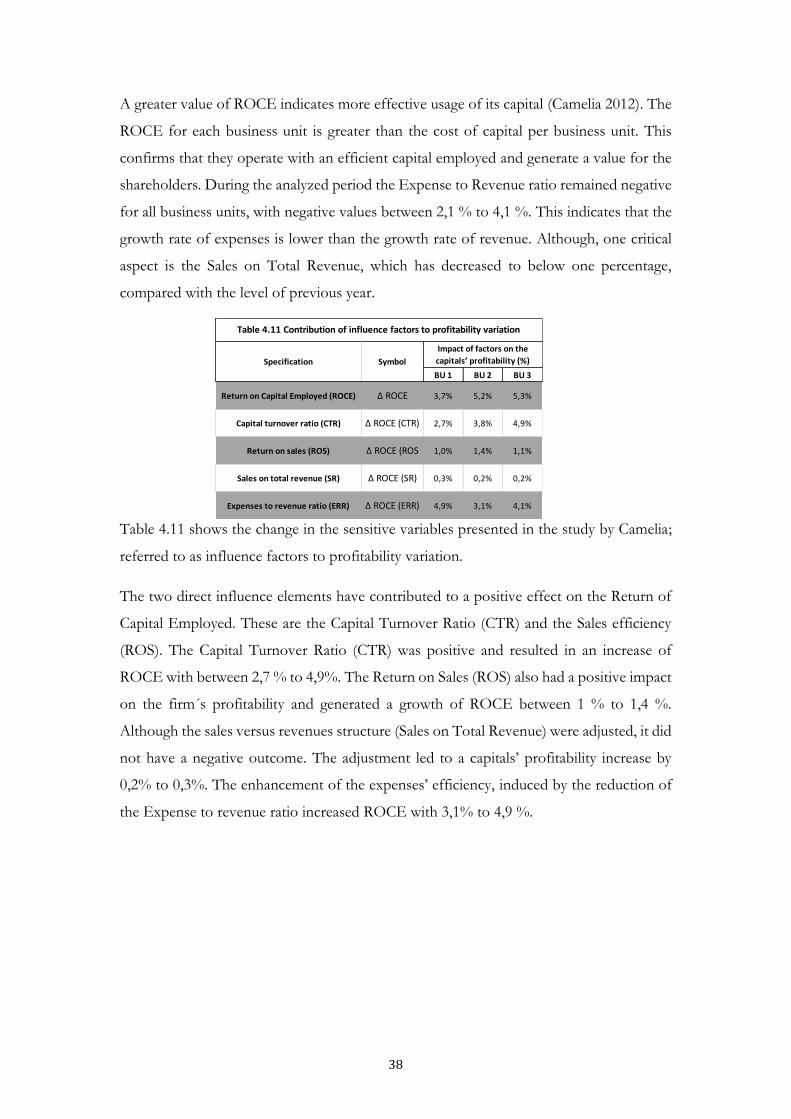
38
A greater value of ROCE indicates more effective usage of its capital (Camelia 2012). The
ROCE for each business unit is greater than the cost of capital per business unit. This
confirms that they operate with an efficient capital employed and generate a value for the
shareholders. During the analyzed period the Expense to Revenue ratio remained negative
for all business units, with negative values between 2,1 % to 4,1 %. This indicates that the
growth rate of expenses is lower than the growth rate of revenue. Although, one critical
aspect is the Sales on Total Revenue, which has decreased to below one percentage,
compared with the level of previous year.
Table 4.11 shows the change in the sensitive variables presented in the study by Camelia;
referred to as influence factors to profitability variation.
The two direct influence elements have contributed to a positive effect on the Return of
Capital Employed. These are the Capital Turnover Ratio (CTR) and the Sales efficiency
(ROS). The Capital Turnover Ratio (CTR) was positive and resulted in an increase of
ROCE with between 2,7 % to 4,9%. The Return on Sales (ROS) also had a positive impact
on the firm´s profitability and generated a growth of ROCE between 1 % to 1,4 %.
Although the sales versus revenues structure (Sales on Total Revenue) were adjusted, it did
not have a negative outcome. The adjustment led to a capitals’ profitability increase by
0,2% to 0,3%. The enhancement of the expenses’ efficiency, induced by the reduction of
the Expense to revenue ratio increased ROCE with 3,1% to 4,9 %.
BU 1 BU 2 BU 3
Return on Capital Employed (ROCE) Δ ROCE 3,7% 5,2% 5,3%
Capital turnover ratio (CTR) Δ ROCE (CTR) 2,7% 3,8% 4,9%
Return on sales (ROS) Δ ROCE (ROS 1,0% 1,4% 1,1%
Sales on total revenue (SR) Δ ROCE (SR) 0,3% 0,2% 0,2%
Expenses to revenue ratio (ERR) Δ ROCE (ERR) 4,9% 3,1% 4,1%
Specification Symbol
Impact of factors on the
capitals’ profitability (%)
Table 4.11 Contribution of influence factors to profitability variation

39
5. ANALYSIS
This chapter initially discusses how the results from section four relate to the relationship between cash flow
and operational capital employed when focusing on increasing firm value. Furthermore, it gives insights in
possible changes for a more efficient operating valuation and forecasting process.
This study was made to investigate the creation of a simpler model used to valuate cash
flow and to show the relationship between cash flow and ROCE. Regarding the new cash
flow model, the result of the study shows that it did not hold for consistency of 100 %
each month. Although, when looking on yearly basis both model 1 and 2 do show a better
result, especially when taking the material COGS into consideration. The interviews
presented a new perspective on material COGS that partly explained why the models do
not hold. A weak integrated system as well as a poor flow of information between business
units and managers disfavor the forecasted values. Because of the poor integrated system
and lack of time we were not able to investigate the material COGS further. Although, it
would have been interesting to see how much of the material COGS that actually should
be charged each month to affect the Cash Flow. Due to our limitations in time and
information, we have chosen to deeper investigate the parts of the study where we have
reached more information. Therefore, the analysis will focus on the sensitive variables
determining cash flow and ROCE.
Firstly, we will discuss and choose one of our cash flow model suggestions. This model
will be investigated and compared to the classic FCF model through a sensitivity analysis.
This will explain how different variables will influence the chosen model compared to the
real FCF model. The cash flow part will be more deeply discussed in part 5.1. Furthermore,
a sensitivity analysis has also been done on the capital employed part. In chapter 4.4 we
did obtain a result equal to the earlier research made by Camelia. This result will be
discussed, criticized and compared to other researches on the subject in chapter 5.2.
Finally, we will use sensitivity analysis together with tornado charts to discuss how different
parameters influence cash flow and ROCE.
5.1 CASH FLOW FORECASTING ON BUSINESS UNIT LEVEL
Ruback (2000), Vishwanath (2009) and Hassani and Misaghi (2013) highlight the
importance of cash flow as a benchmark of the firm’s ability to cover operational expenses.
Vishwanath means that cash flow forecasting could both be used to measure the firm’s
performance and to find possibilities of adding value. Almeida, Campello and Weisbach

40
state “cash flow forecasting is crucial for the firm. It contributes to security regarding resources and
operational expenses, which gives confidence to project managers”. This might be one explanation of
the poor performance by project managers regarding budgeting their projects. According
to the financial manager at our investigated firm, the firm is in great need of a well
functioning system for cash flow forecasting. The non-functional structure used today may
disfavor the decision making by project managers, which was proven further on in the
interviews with project managers.
With this said, the estimation of cash flow is extremely important. Being able to forecast
cash flows already on business unit level would make an even greater contribution to final
firm value, according to the financial manager at out investigated firm. Interestingly, even
if firms do have practical needs for cash flow models on lower unit levels there are no
notable previous researches in this area. Vishwanath’s study shows the initial classical FCF
calculation, but there are limitations for doing this at business unit level.
It is important to also consider the negative arguments regarding cash flow forecasting.
McInnis and Collins state “cash flow forecasting may not only be positive. The transparency forced by
forecasting does diminish the firm’s ability to control future earnings”. McInnis and Collins do have
a point here, although we believe that the arguments strengthening cash flow forecasting
are stronger than the negative aspects.
5.1.1 COMPARISON OF MODEL 1 AND 2
When investigating our first research question “is it possible to create a simpler model for forecasting
cash flow per business unit?”, yes would be the simple answer. Although, we found that the
action of creating this model is not that simple. In this question we have arrived at two
different model suggestions, which are shown in table 3.1. The difference between
monthly and average, is to see whether the average will capture fluctuations in a better way.
Table 3.1 Suggestions of models for forecasting cash flow:
Cash Flow Model 1 Cash Flow Model 2
Monthly Incoming Payments Monthly Incoming Payments - Project COGS Monthly - Project COGS Monthly - Other COGS Average - Other COGS Monthly - OPEX Average - OPEX Monthly = Cash Flow = Cash Flow
After investigating the suggested models we have come to the conclusion that none of the
models hold perfectly for every month (see table 4.1. and 4.3). The further question is now

41
how we can change the model to reach a better percentage of consistency, in line with the
classic FCF model?
The previous research by Hassani and Misaghi states “it is important to find a balance between
gains and losses when using a simplified model for forecasting cash flow. Therefore, the firm has to find the
level where the loss in cash flow forecast accuracy is equal or more than the increase in profitability”. This
means that although the new model suggestion is not perfect is may still result in increased
profitability. According to the financial manager at our investigated firm, they would lower
the operational expenses if using a simpler model. Although, these savings must benefit
the profitability enough to increase cash flow. As presented in Hassani and Misaghi’s
research “profitability and capital employed are main factors when determining operational cash flow”.
This means that by increasing efficiency on these variables the firm would also increase its
operational cash flow. The chain reaction proves that the use of a simpler valuation model
will be profitable for the firm, if it reaches a cash flow outcome close enough to the classic
FCF model.
Previous research by Dastgir, Khodadadi & Ghayed states “the valuation of the firm becomes
an important tool, which can contribute to the value of the firm; because the cash flow available for
shareholders will increase as the value of the firm increases”. This together with Hassani and
Misaghi’s findings on cash flow and profitability could drive the creation of a simpler cash
flow model.
In both model 1 and 2 the percentage of consistency did occasionally reach up to 100 %,
but fluctuated between the months. This means that even though the result for each month
was not good enough (see table 4.1 and 4.3), the yearly ratio could be a valuable tool for
the estimation if it catches up the correlation. The p-value tells us that the correlation for
the both models is below 1 % and thereby has a high level of significance.
Both models use monthly values for payments and project COGS, which is why the
models reach the same result when considering the weight of material COGS not affecting
cash flow. The deeper analysis of material COGS as a part of project COGS reached the
lowest change of result for business unit 1. This business unit also reached the best results
in percentage of consistency throughout the whole study. Furthermore, business unit 2
and 3 reached lower results and also have a higher degree of material as a percentage of
the project COGS. This proves that the weight of material COGS is one of the major
reasons for the failure of the two models. The interviews with project managers also

42
strengthen this conclusion. The results of the interviews show a gap in flow of information
between the logistics department and the project managers. Logically, this gap will
contribute to a deeper loss if the project managers at one business unit deal with more
material within their projects. In some of the periods the average percentage of material
COGS reached over 90 %. As the interviews with the project managers showed a poor
communication structure, it is not hard to believe that not all of the material where bought
in that period. We also investigated and found that there is no connection between having
an extremely high material COGS and high sales.
The limited information regarding the date of payment of material and how the
investigated firm place orders did prevent us from a deeper analysis. Information regarding
how they place orders would be of great interest. For example if they favour few but large
order this would have an effect on the material cogs, cash flow and so our model. Due to
our limitation of information we can only state that from the information that we have
access to, it is likely that both models would be improved if considering the material COGS
of the project. The company should therefore consider implementing a logistics system,
by which managers easily can trace the material. This would not only help to improve the
cash flow model, it would also provide managers with valuable information such as stock
levels of different components. This would improve the co-operation with clients and it
would be easier for the managers to decrease costs and the cash out flow.
Which of the two models is then the best to use?
Both model use monthly values for payments and project COGS, but they do differ
regarding the other COGS and expenses. When looking at table 4.5, model 2 reaches a
higher average, but model 1 reaches a higher amount of months with over 90 %
consistency. In this question it is important to remember that other variables also affect
the result of each month. If we had been able to look at a longer time horizon, we would
have been able to determine whether the result followed the seasonal fluctuation and other
trends. If this was not the case, it could be one explanation of why model 1 sometimes
gives a more accurate percentage of consistency. This is one possible explanation, however,
it is difficult for us to draw any definite conclusion because of the lack of information.
When comparing the two models in table 4.6, model 1 reaches the same or a higher average
in all of the parameters except the volatility. As we mentioned before, both models show
good values on yearly basis and good correlation, which could be seen as stronger factors
than volatility. According to our comparison, model 1 should be chosen if the firm is
43
satisfied to use the model as guidance on yearly basis or uses monthly average which are
based from yearly numbers. Even though model 1 reaches a 100 % of consistency for
business unit 1 on yearly basis, it is hard to tell if the model would be considered the best
representative for other business units and other firms.
It is difficult to tell why neither of the models do not hold for business unit 2 and 3.
Possible reasons could be due to unusual fluctuations or payments that were paid either
too late or too early. The exchange rate may affect the business units differently because
they operate in different regions. Furthermore, we must not forget our limitation with the
time horizon. Since we only were able to look deeply into the year of 2014, it is hard to tell
how the models would perform when considering a longer time horizon. A longer time
period would make it easier to find unusual fluctuations and variations between the months
and years. This data would be essential for future investigation on creating a model for
forecasting cash flow on business unit level.
According to the financial manager at our investigated firm, the market practically does
demand a simpler model for forecasting cash flow on business unit level. This demand
could be used as one of the driving arguments for developing this kind of model. Even if
we have not been able to reach a final solution in this study, we have come to conclusions
regarding yearly guidelines for forecasting cash flow on lower levels.
How good does the model need to be, before it would create value to the firm?
By reviewing Vishwanath’s study on the classical FCF model, we come to the conclusion
that when creating a simpler model there will be a difference in final cash flow outcome.
Although this does not mean creating a simpler model would be impossible. According to
both the previous research by Hassani and Misaghi and the financial manager at our
investigated firm, the creation of such a model would still be beneficial. With that said, it
is important to compare the increase in profitability and the loss in forecast accuracy when
using a simpler model. Hassani and Misaghi states that this relation should be considered
when working with operational cash flow. According to the financial manager at our
investigated firm, they would be satisfied with a level between 80 – 90 % of consistency.
At this level they would reach a balance between the increase in profitability and loss in
accuracy, stated by Hassani and Misaghi. At this point our recommendation would be to
use our model on yearly basis. Furthermore, the model could be used on monthly basis as
an average from the yearly basis to still reach a minimum of 80 % consistency.

44
After comparing our results with previous research we have come to the conclusion that
the use of model 1 would be preferable. This model provides the same result when looking
on yearly basis and a better result when looking at monthly average and the correlation.
Model 2 does reach a similar result, but with a lower correlation.
The differences between model 1 and model 2 are found in the two last variables: other
COGS and expenses. In these variables, model 1 uses an average of the ten periods and
model 2 uses monthly estimation. Other COGS and expenses do not constitute a large
portion of the total expenses, compared to the project COGS. They are therefore not as
important to be looked at on monthly basis as the project COGS. When looking at the
fluctuations from month to month, we recognize most fluctuations in the project COGS
and the two other expense variables are quite stable over time. By using the average it is
also possible to catch the seasonal fluctuations. Ruback and Vishwanatha’s critique
concerning the calculation difficulties would also be satisfied since model 1 includes simple
calculations.
5.1.2 SENSITIVITY ANALYSIS BETWEEN MODEL 1 AND REAL FCF MODEL
In this part of the analysis we will use the sensitivity analysis approach to deeper investigate
the four following variables: Incoming payments/sales, project COGS, other COGS and operational
expenses (OPEX). This will show the sensitivity of our model compared to the classic FCF
model. In this section, we have chosen to only discuss model 1 as it have proven to have
a better outcome than model 2.
The reason why we have chosen the four variables is because they will affect both models.
The limitation is that the real FCF model does not consider incoming payments and our
model does not consider sales. The firm uses an invoicing period of 30 days and they have
an average of 20 days before they get their payment. This is the only way to compare the
first variable between the two models. Therefore one need to be critical concerning the
outcome of this variable.
Our model and the classis FCF model should in a perfect scenario show the same
adjustment in percentage. This was not achieved in this study. According Vishwanath “there
will be a difference in final cash flow outcome”, which was confirmed by our results. The exact
same value of cash flow can only be reached if both models would have the same outcome
of the cash flow before any adjustments are made. This because values of the adjustment
45
will be presented as in percentage of change compared to the value before any adjustment
is made. This limitation of the sensitivity analysis must be considered.
Table 5.1 describes how the model 1 and the real model are affected when changing the
four variables with an increase and decrease of 10 %. The table shows the change
percentage of the total outcome of cash flow that will be changed compared to the
outcome before adjustment. According to our earlier result on the percentage of
consistency, business unit 1 reached 100 %, business unit 2 79 % and business unit 3 72
% (see table 4.2). Our model should follow these results and react similarly to the real FCF
model. Business unit 1 with 100 % consistency should be the only business unit to reach
the exact same analytical result as the real FCF model. This is supported by the value of
100 % consistency before any adjustments.
By changing the first variable we can see a difference in influence on our model and the
classic FCF model. The effect becomes greater on the classic FCF model which
considering sales, compared to our model which is considering incoming payment. A
possible explanation for this is that the incoming payments are not equal to the sales.
Furthermore, the cash flow outcome before was not identical in all business units.
Considering business unit 1, the difference between the two models may be explained by
the lack of co-variation between incoming payments and sales. When considering the
results for the other three variables, we see almost the exact same result in business unit 1
as in the real FCF model. The only difference is found in project COGS, where there is a
difference of one percentage. This speaks for our model’s ability to catch the fluctuations
in these project COGS, other COGS and OPEX.
Considering business unit 2 and 3, we can see that the results from our model are close to
the result from the real FCF model; with a difference of 0 % - 3 %. A possible explanation
is the difference between the real model and model 1 before any adjustment. Business unit
2 only reached 79 % consistency and business unit 3 72 % consistency before the
adjustment. Another possible consideration is that business unit 3 holds higher sales than
Real Model Model 1 Real Model Model 1 Real Model Model 1
Δ 10 % Incoming payments / Sales 38% 22% 29% 25% 52% 38%
Δ 10 % Project Cogs 18% 19% 22% 18% 28% 26%
Δ 10 % Other Cogs 1% 1% 2% 2% 0% 0%
Δ 10 % OPEX 7% 7% 21% 18% 12% 9%
Business Unit 1 Business Unit 2 Business Unit 3Indicator - Sensitivty as a
percentage
Table 5.1 Sensitivty Analysis Model 1 vs Real Model on yearly basis (Jan - Dec 2014)

46
the other business units in relation to the incoming payments for this specific period.
Customers placing orders in December to lower their result and avoid taxes or other
incentives may explain this. This will lead to sales affecting the year of 2014. Instead, the
incoming payments will arrive in January and therefore affect the year of 2015.
According to the result from table 5.1 we can tell that our model shows a good result and
catches up the changes in the variables compared to the real FCF model, but implications
are found when forecasting payments/sales. Further improvement of the model would be
to investigate the correlation between the payments and the sales at a longer period. Even
if our model does reach a good result we have to be critical and also consider the variation
of other variables. Variables such as depreciation, capital expenses and working capital are
not included in the sensitivity analysis. Although, our model does catch up the effect of
these variables, e.g. the depreciation will affect the income statement, which will affect the
expenses. Alternative, other cogs, capital expenses and working capital would affect the
incoming or outgoing payments.
The sensitivity analysis in table 5.1 does not show how the total outcome (percentage of
consistency) would be affected when changing the variables. Table 5.2 will therefore be
used to clarify this question. This will measure how good the two models co-vary at a yearly
basis.
In table 5.2 the indicator before adjustment shows the percentage of consistency on yearly
basis before any adjustment is done. This table shows if the result in table 5.1 can be
motivated or not. E.g. for business unit 1 which has a percentage of consistency of 100 %,
then if the variations in percentage is close to each other, the result in table 5.2 also should
be close to each other. Regarding business unit 1 in table 5.2, the last three variables show
a good result by almost reaching a 100 % match. The first variable “Incoming payment /
Sales” does fluctuate when we increase or decrease the variables and the outcome does
differ compared to before the adjustment. This is explained by the difference between our
model and the real FCF model, which is also showed in table 5.1. Regarding business unit
Increase Decrease Increase Decrease Increase Decrease
Before adjustment
Δ 10 % Incoming payments / Sales 79% 88% 88% 71% 52% 50%
Δ 10 % Project Cogs 100% 99% 75% 84% 78% 76%
Δ 10 % Other Cogs 99% 99% 78% 79% 71% 71%
Δ 10 % OPEX 99% 99% 75% 84% 69% 75%
Table 5.2 Sensitivty Analysis on yearly basis (Jan - Dec 2014) - Model 1
Indicator - Percentage of
Consistency
Business Unit 1 Business Unit 2 Business Unit 3
100% 79% 72%

47
2 and 3, there is also a difference in value. This can be explained by the results from table
5.1, but also by the percentage of consistency that was not 100 % before the adjustment.
As proved in the two sensitivity analyses (table 5.1 and 5.2) our model does give a 72-100%
of consistency when considering variations in the four variables. Especially business unit
1 does reach a good result. Even though this is a high percentage for business unit 1, the
other two business units do not reach the satisfied level of 80-90 % of consistency, set by
the investigated firm. This highlights the complicity of creating a cash flow forecasting
model suitable for different business units within a complex firm. Also, we must consider
if the investigated business units can represent all units at the firm. Because of our
limitations in time and information we will not be able to complete the creation of an
efficient forecasting model on business unit level but we have contributed with a giving
discussion on the subject. The suggested model did hold for one of the business units.
Therefore it cannot be fully rejected. The recommendation for our investigated firm would
be to firstly improve the communication and then redo the research including more
business units during a longer time period. These guidelines would also be applicable for
other complex firms with similar problems in cash flow forecasting.
5.2 ANALYSIS OF PROFITABILITY OF CAPITAL EMPLOYED (ROCE)
When investigating our second research question “how sensitive are the different variables
determining capital employed and how could they be changed in order to increase firm value?” we have
chosen to follow the same working process as Camelia. By continuously comparing our
result to previous research, we will ensure reliability.
Our result regarding the variable sensitivity of capital employed is in line with previous
research. Hassani and Misaghi, Camelia and Wallace highlight the importance to focus on
profitability. Profitability as one of the major variables when aiming to increase firm value
was confirmed in our result (table 4.10) where we see a positive change in all variables
affecting ROCE. When estimating the firm’s performance, we found that, during the
investigated year, each of the business units has improved the potential of economic
financial growth. This is verifying that there are real capacities to create capital value with
efficiency, which also increases firm value.
Both Wallace and Camelia states “the factors that influence a company’s capital profitability are
several and strongly related to the external and internal restrictions of the firm. The firm needs to manage
their resources in an efficient way in order to be capable to generate value”. Wallace means “this should

48
be the first area to review when it comes to increasing profit or reducing costs”. One interesting aspect
in our results is the confirmation of the poor communication system and flow of
information within our investigated firm. This again is another argument for the firm to
focus on this kind of problems.
In line with Camelia’s study, our investigation of the profitability of capital employed
(ROCE) has shown vital parts, which have to be considered from the managerial decisions
regarding how to run the company to achieve the best profitability (table 4.11). According
to Wallace, “an efficient management is an essential aspect for enhancing the economic-financial potential
of the company and it needs to be reflected in all of the production factors used in the operation”. The firm
can only reach profitability when it is able to use its resources in a good way; receiving
revenues that exceeds expenses. As presented in the result (table 4.11) the indicator ERR,
shows that the efficiency of expenses will have a direct influence of the profitability.
According to Camelia, “one factor with tremendous significance for the company is how efficient and
effective a company is with their commercialization activity, to be able to meet the competitive environment”.
The indicator Return on Sales proposes that a company’s efficiency will increase along
with enhancement in the resource allocation. This means that they both need to increase
their sales’ share in the total revenues and reducing the expenses to revenue ratio. This is
confirmed in our study (table 4.11). The growth rate of a company is highly related with
the influence of the important factor. In our study the growth rate is measured as the
Capital Turnover ratio (CTR). A usage with a superior efficiency of capitals is suggested to
lead to an improved yield for investors, which is also confirmed in our study.
The different influence factors on profitability will be affected with limitation related to
the characteristics of the competitive environment. The interviews with project managers
and the financial manager supports this conclusion. Our results are here is in line with
Wallace’s study, which highlights the importance of managerial structure and development.
By identifying the influence factors and possessing knowledge on their action and
relationship, the firm will be more efficient in their monitoring. This is also strengthened
by the research by Almeida, Campello and Weisbach. This research states that increased
security within the firm will increase the confidence and courage of decision makers, which
in turn will be beneficial for the firm.
Regarding the profitability of capital employed, we have come to the same conclusion as
Camelia. Additionally, this study has considered critique and arguments from other
49
researches on the subject in order to develop new perspectives. This study considered
different quantitative and qualitative data, as well as a different time period than Camelia,
which will ensure reliability and validity of the study.
5.3 THE RELATIONSHIP BETWEEN CASH FLOW AND CAPITAL EMPLOYED
To analyze the relationship between ROCE and cash flow we will use sensitivity analysis.
Regarding this relationship, our results are in line with previous research. Hassani and
Misaghi states “there is a meaningful relationship between capital employed and operational cash flow.
By reducing capital employed one will reach a lower weighted average cost of capital. This is followed by an
increased value of cash flow, which in turn will increase the value of the firm”. Wallace and Camelia
also discuss this chain reaction. They use the perspective of internal resources allocated
towards increased firm value. Furthermore, our results from the interviews with project
managers and the financial manager have highlighted the importance of working with both
cash flow and capital employed. Previous research by Dastgir, Khodadadi & Ghayed states
“the valuation of the firm becomes an important tool, which can contribute to the value of the firm”. This
together with Almeida, Campello and Weisbach’s research on the sensitivity of cash flow
could be seen as one argument for the relationship between cash flow and firm value.
According to Camelia, Wallace and Hassani and Misaghi, ROCE is also linked to firm
value, which strengthens the relationship between ROCE and cash flow. According to
Camelia “expectations by stakeholders are also a driving factor concerning the appreciation of capital
employed”. Interestingly, expectations by shareholders are one important factor regarding
cash flow and firm value as well. Regarding cash flow forecasting, Hassani and Misaghi
presents the strongest argument for the relationship between cash flow and capital
employed. By using their model we see the direct linkage between the two variables. The
model proves that it is important to find a balance between gains and losses when using a
simplified model for forecasting cash flow. Hassani and Misaghi state “the firm has to find
the level where the loss in cash flow forecast accuracy is equal or more than the increase in profitability”.
This is why we, in this study, have chosen to focus on the investigation of the variable
profitability. This variable is not only one of the determining variables when measuring cash
flow; it also affects capital employed. This makes profitability one of the most important
factors to look at for firms wanting to increase its cash flow, ROCE and firm value. As
firm value is closely linked to the value of the firm’s cash flow the understanding of this
relationship becomes major important.
50
Table 5.3 presents the sensitivity analysis of the variables determining ROCE and cash
flow. In this model, we have chosen different variables than used before in model 5.1 and
5.2: Sales, Expense and Capitals. The change in variables are motivated by the need of
finding variables influencing both ROCE and cash flow. In the real FCF model, sales and
expenses affect cash flow through the profit (EBIT). The influence of capital investments
is found in working capitals or capital expenditure. Our cash flow model is influenced by
sales when considering the incoming payments. In the sensitivity analysis (table 5.3),
expense Capital investments are affecting through outgoing payment, which reduces our
incoming payment.
An increase in sales will lead to an increase in EBIT, which further on will affect the cash
flow in a positive way. The increase in sales also increases the return on capital, return on
sales and other factors that contributes to an improvement in ROCE. Expenses do have a
negative influence on the cash flow as for the ROCE. This linkage is in line with previous
research by Hassani and Misaghi.
Table 5.3 presents the effect on ROCE and Cash flow when changing the variables with
10 %. The results are shown in percentage and will thereby be the same for an increase as
for a decrease. The table shows that the change in sales has the greatest influence on both
ROCE and Cash Flow. Interestingly, according to Camelia “the firm’s profitability will increase
together with the improvements of efficiency in the production and commercialization activity”. This could
be seen as changes in line with increasing sales, which strengthens the result of the
sensitivity analysis.
One must not forget that these results could be different regarding different firms and
industries. If you analyse a company with low sales but high amount of capitals, the result
would be different. The results from the table show us that both the cash flow and ROCE
will be affected by changes in the three variables. In this model the cash flow will be
BU 1 BU 2 BU 3
22,4% 31,2% 26,5%
Δ ROCE 12,0% 14,0% 17,0%
Δ Cash flow 38% 29% 52%
Δ ROCE 9,0% 11,0% 13,0%
Δ Cash flow 20,0% 25,0% 32,0%
Δ ROCE 1,5% 3,0% 3,0%
Δ Cash flow 7,4% 9,3% 10,5%
Indicator
Table 5.3 Sensitivty Analysis ROCE vs Cash Flow
Current ROCE
Δ 10 % Sales
Δ 10 % Expense
Δ 10 % Capitals
51
affected more, since these parameters do have a more direct influence on cash flow. When
calculating the ROCE, the effect will reach through other variables, as is describe in
method 3.5.2. The effect on ROCE will therefore not be as strong as the effect on cash
flow.
The effects from table 5.3 is graphically displayed in the tornado charts below, where
diagram 5.1 represents business unit 1, 5.2 business unit 2 and 5.3 business unit 3.
The tornado charts show the effect when varying the different variables. The variable that
has the strongest effect on the outcome is placed in the top of the graph and the one with
the least effect in the bottom. The starting value is placed in the middle of the graph. The
dark shaded area displays the result when increasing or decreasing the variables. The
tornado charts are chosen as they easily illustrates the result from the sensitivity analyses.
The tornado charts only illustrate the result from the ROCE part of table 5.3. The FCF
part will not be illustrated due to difficulties created by confidential information.
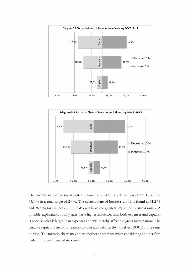
52
The current state of business unit 1 is found at 22,4 %, which will vary from 17,3 % to
34,4 % in a total range of 24 %. The current state of business unit 2 is found at 31,2 %
and 26,5 % for business unit 3. Sales will have the greatest impact on business unit 3. A
possible explanation of why sales has a higher influence, than both expenses and capitals,
is because sales is larger than expenses and will thereby affect the gross margin more. The
variable capitals is minor in relation to sales and will thereby not affect ROCE in the same
portion. The tornado charts may show another appearance when considering another firm
with a different financial structure.

53
In this study, we have reached a conclusion that proves the theory by Hassani and Misaghi
on the relationship between cash flow and capital employed. This theory has also been
criticized and discussed through the perspective of other researches, such as Camelia and
Wallace. By increasing variables that affect the ROCE and profitability, one will also affect
the cash flow.

54
6. CONCLUSION
In the final chapter, the conclusions of our study will be presented. Finally, suggestions for further research
will be given on the subject.
After our investigation of cash flow and capital employed, we have come to the conclusion
that it is possible to create a simpler cash flow model, yet there are complications. Although
none of the two models did reach a perfect result on monthly basis, they both showed
good results on yearly basis. Consideration is needed regarding the validity of the two
models since they are based on the period of year 2014 and at only three business units.
Nevertheless, based on our study model 1 is preferred due to its high average of
consistency, and it is recommended to be used on a yearly basis. However, there are
limitations and possible factors that may have affected our findings, which must be taken
into consideration.
The short time period of data and the poor flow of information within the firm limited us
from carrying out a deeper analysis regarding the monthly fluctuations. The deeper look
would have revealed how much the material COGS affect the incoming payments and
how the model would respond in a longer time horizon. This information would have been
valuable for making adjustment for improving our model. Given that the firm wanted at
least 80 % of consistency for implementing the model, when looking on a yearly basis, the
model only reached this level for one of the three business units. Considering this, the
model should be tested for a longer time period and analyzed further before being
implemented. Furthermore, as the comparison of the impact on model 1 and the real FCF
model, when changing different variables, revealed a good connection for all variables
except “sales / incoming payments”, this proves that the model will work to a certain
point. However, as mentioned before an improvement is needed for a better result.
The study has proved the connection between capital employed and cash flow which is
mentioned in earlier research. It has also proven that there are four important parameters
that positively affect ROCE such as Capital Turnover Ratio, Return on Sales, Sales on
Total Revenue and Expenses to Revenue Ratio. The firm should therefore focus on these
variables by purpose in order to increase its firm value.
By letting the manager at the lower level constantly work with variables that both affect
ROCE and cash flow, the interest of the shareholders regarding value maximization will
be fulfilled.

55
From our qualitative part of the study we found that there is a shortage regarding the flow
of information between different departments. By implementing a system that increases
the flow of information, it will make it easier for the management to further increase its
cash flow and return on capital employed.
6.1 PRACTICAL AND THEORETICAL CONTRIBUTIONS
The study has contributed to practical guidance by creating a new model for cash flow
calculations. Even though it is not perfect, it represents a good start to future research.
This study could be used as guidelines for further practice where other firms may create
the model suggestion to be more suitable for the specific firm. Furthermore, the proved
relationship between cash flow and capital employed highlights it as an important
connection to work with in order to increase firm value.
6.2 FURTHER RESEARCH PROPOSAL
The problems we have faced due to lack of information, have been to a disfavour for the
creation of the cash flow model. It would therefore be of great interest to analyse the
model even deeper including more information during a longer time horizon. It would be
of great interest if our model, or an improvement of our model, would be tested in
different types of firms. Especially where the factors mentioned in our “Model Critique”
in chapter 4.1.3 could be eliminated. Finally, it would be interesting to analyse how firms
work with their cash flow and return on capital employed. If they constantly work with
maximization of these variables and if the management at lower business levels possess
the knowledge of the relationship that exist.

56
REFERENCES
LITERARY SOURCES
Almeida Heitor, Murillo Campello and Michael S. Weisbach. ‘The Cash Flow Sensitivity
of Cash’. The Journal of Finance Vol. 59 No.4 (2004): 1777-1804. Print.
Bryman, Alan, and Emma Bell. Business Research Methods. Oxford: Oxford University Press.
(2009). Print.
Camelia, Burja. 'Analysis Model For Return On Capital Employed'. University of Târgu Jiu
Economy Series Issue 1 (2013): 82-87. Print.
Collis, Jill, and Roger Hussey. Business Research. Houndmills, Basingstoke, Hampshire: Palgrave
Macmillan, 2003. Print.
Damodaran, Ashwath. Return On Capital (ROC), Return On Invested Capital (ROIC)
And Return On Equity (ROE): Measurement And Implications. Stern School of Business,
2007. Print.
Dastgir, Mohsen, Vali Khodadadi, and Maryam Ghayed. 'Cash Flow Valuation Using
Capital Cash Flow Method Comparing It With Free Cash Flow Method And Adjusted
Present Value Method In Companies Listed On The Tehran Stock Exchange'. Business
Intelligencen Journal (2010): 45-55. Print.
Ismail, Idris, Daniil Nilsson, and Rami Bou-Hamdan. Informationsasymmetri På Finansiella
Marknaden. Mälardalen: Mälardalen University, 2015. Print.
Kaplan, Steven N., and Richard S. Ruback. 'The Valuation Of Cash Flow Forecasts: An
Empirical Analysis'. National Bureau of Economic Research Working Paper No. 4724 (1994):
33-35. Print.
McInnis, John, Daniel W. Collins. ‘The Effect of Cash Flow Forecasting on Accrual
Quality and Benchmark Beating’. Journal of Accounting and Economics Vol 51 (2011): 219-239.
Print.
Research Firm,. Balance Sheet Statement. 2014. Confidential document. Gothenburg.
Research Firm,. Cash Flow Statement Of Business Unit 1. 2014. Confidential document.
Gothenburg.

57
Research Firm,. Cash Flow Statement Of Business Unit 2. 2014. Confidential document.
Gothenburg.
Research Firm,. Cash Flow Statement Of Business Unit 3. 2014. Confidential document.
Gothenburg.
Research Firm,. Income Statement. 2014. Confidential document. Gothenburg.
Tsiang, S.C. 'The Rationale Of The Mean-Standard Deviation Analysis, Skewness
Preference, And The Demand For Money'. The American Economic Review Vol. 62.3 (1972):
354-371. Print.
Vishwanath, S. R, and Chandrashekar Krishnamurti. Investment Management. Berlin:
Springer, 2009. Print.
Wallace, Davis. Return On Capital Employed: Review Of The NZ Listed Sector. Armillary
Private Capital, 2015. Print.
INTERNET SOURCES
E-conomic.se,. 'Sysselsatt Kapital – Vad Är Sysselsatt Kapital? | E-Conomic'. N.p., 2015.
Web. 2 July 2015. https://www.e-conomic.se/bokforingsprogram/ordlista/sysselsatt-
kapital
Investopedia,. 'Stakeholder Definition | Investopedia'. N.p., 2003. Web. 2 July 2015.
http://www.investopedia.com/terms/s/stakeholder.asp
ORAL SOURCES
Research Firm, Financial Managers, Business Unit 1. Interview Cash and its impact On
Business Unit Level. 22-04-2015. in person.
Research Firm, Financial Managers, Business Unit 2. . Interview Cash and its impact On
Business Unit Level. 23-04-2015. in person.
Research Firm, Financial Managers, Business Unit 3. . Interview Cash and its impact On
Business Unit Level. 24-04-2015. in person.
Research Firm, Project Managers, Business Unit 1. Interview On Flow Of Information
And Communication On Business Unit Level. 07-05-2015. in person.
58
Research Firm, Project Managers, Business Unit 2. Interview On Flow Of Information
And Communication On Business Unit Level. 09-05-2015. in person.
Research Firm, Project Managers, Business Unit 3. Interview On Flow Of Information
And Communication On Business Unit Level. 11-05-2015. in person.
WEB SOURCES
Gelman, Andrew. 'P Values And Statistical Practice'. Epidemiology 24.1 (2013): 69-72. Web.
2015-05-28
Hassani, Mohammad, and Mehri Misaghi. 'A Study On Relationship Between Capital
Employed Efficiency And Operating Cash Flow: Evidence From Tehran Stock Exchange'.
10.5267/j.msl 3.4 (2013): 1089-1094. Web. 2015-05-27
Ruback, Richard S. 'Capital Cash Flows: A Simple Approach To Valuing Risky Cash
Flows'. SSRN Journal (2000). Web. 2015-05-27

59
APPENDIX 1 - INTERVIEW QUESTIONS: FINANCIAL MANAGERS
How do you operate today with cash flow calculation?
What disadvantages do you find with todays approach?
What advantages do you find with an easier way of measuring the Cash Flow?
Which variables do find important to consider in a new Cash Flow model?
How do the managers at lower business unit levels work with cash flow?
How good does the new model need to be before you would consider implementing it?
APPENDIX 2 - INTERVIEW QUESTIONS: FLOW OF INFORMATION,
PROJECT MANAGERS
Cooperation is one of the cornerstones of project management - what does collaboration
mean to you?
How do you handle communication with different parts of the business before, during and
after the project?
As a manager, is it possible for you to get information regarding when the different material
is bought and stored in the logistics department? If so, is it an easy or complex procedure?
Please specify.
Is there any part of the communication between the units you think should be improved?
Do you feel like you can provide enough information about the project from / to other
units involved in the project? If no, how do you think this could be improved?
Do you follow up the project and make communication improvements?
Do you think the company is working enough to improved communication?
Are you aware of how enhanced communications could improve your work situation?