CASH BY ANY OTHER NAME EVIDENCE ON LABELLING FROM

THE UK WINTER FUEL PAYMENT

Timothy KM Beatty University of Minnesota

Laura Blow Institute for Fiscal Studies

Thomas F Crossley University of Cambridge Institute for Fiscal Studies and Koccedil University

Cormac OrsquoDea Institute for Fiscal Studies

Abstract Government transfers to individuals are often given labels indicating that they are designed to support the consumption of particular goods Standard economic theory implies that the labelling of cash transfers or cash-equivalents should have no effect on spending patterns We study the UK Winter Fuel Payment a cash transfer to older households Our empirical strategy nests a regression discontinuity design with an Engel curve framework We find robust evidence of a behavioural effect of labelling On average households spend 41 of the WFP on fuel If the payment were treated as cash we would expect households to spend 3 of the payment on fuel

Keywords labelling benefits expenditure regression discontinuity JEL codes D12 H24

This research was made possible by a grant from the Nuffield Foundation but the viewsexpressed13 are13 those13 of the13 authors13 and13 not necessarily13 those13 of the13 Foundation Thanks to Sule Alan Mike Brewer Andrew Chesher Dominic Curran Valeacuterie Lechene Gugliemo Weber and participants in a number of seminars for helpful comments Any remainng errors are our own

1

I INTRODUCTION

Government transfers to households and individuals are often given labels indicating

that they are designed to support the consumption of a particular good or service For

example many countries provide transfers to households with children and label them a

ldquoChild Benefitrdquo When such transfers are made in cash there is no obligation to spend all or

even any of the payment on its ostensive purpose Standard economic theory implies that the

label of a particular transfer should have no bearing on how that transfer is ultimately spent

since all income is fungible The recipient of a transfer with a suggestive label is expected to

react in exactly the same way as he would have reacted had he been given a transfer of

equivalent value with a neutral label The receipt of an in-kind transfer such as food stamps is

similar as long as consumers are infra-marginal ndash ie for those whom consumption of the

good in question is already larger than the voucher amount Why then do governments label

transfers Of course one possibility is that doing so makes redistribution more palatable to

voting taxpayers However another intriguing possibility is that standard economic theory is

mistaken on this particular point and spending patterns can be influenced by the labelling of

cash or cash-equivalent transfers In this paper we provide novel evidence on the behavioural

effect of labelling from the UK Winter Fuel Payment (WFP)

The theoretical proposition that labelling is irrelevant has been challenged For

example Thalerrsquos (1990 1999) framework of mental accounts is one mechanism through

which the labelling of a transfer might affect its usage1 There is though very little previous

empirical evidence to support the idea that the labelling of a transfer payment matters

Kooreman (2000) and Blow Walker and Zhu (2010) find evidence that additional

child benefit differs from other income in its effect on household spending patterns among

child benefit recipients in the Netherlands and the UK respectively Kooreman finds some

1 In the present context income would be labelled according to its source and so the Winter Fuel Payment would be allocated to a mental account for spending on heating

2

evidence of a labelling effect (ie the child benefit is spent on child-related goods) in

contrast Blow Walker and Zhursquos results suggest child benefit is spent disproportionately on

adult-related goods2 Finally Edmonds (2002) also looks at child benefit payments (in this

case amongst families in Slovakia) but finds no evidence of a labelling effect These studies

use quasi-experimental difference-in-difference designs exploiting differential changes over

time in the real value of benefits for different types Effects are identified by a common

trends assumption An additional complication is that it is not possible - in two-adult

households - to separately identify a labelling effect of child benefit income from the

alternative explanation that the increase in the share of total household income received by

the mother (child benefit is almost always paid to the mother) leads the change in spending

patterns That is it could be who receives the money rather than the label that matters and

the potential labelling effect cannot be disentangled from a ldquorecipiencyrdquo or intrahousehold

effect This issue of intrahousehold allocation may be particularly important in the case of

spending on children Among single-mother households for whom these intrahousehold

considerations are not relevant Kooreman finds an effect in the direction consistent with

labelling mattering However in his baseline specification the effect is not statistically

different from zero at conventional levels Similarly Blow Walker and Zhu find weaker

results for single-parent households

Turning to in-kind transfers such as food stamps while some researchers have

claimed to find evidence contradicting standard economic theory the studies with the most

credible and convincing designs find the opposite In particular Moffitt (1989) and more

recently Hoynes and Schanzenbach (2009) find no evidence that infra-marginal consumers

treat food stamps differently than an equivalent cash payment

2 This does not imply parents disregard their childrenrsquos welfare The paper finds evidence that this spending effect comes from the unanticipated variation in child benefit which suggests that parents are altruistic and insulate their children from income variation

3

In contrast Abeler and Marklein (2010) have recently compared in-kind grants and

(unlabelled) cash grants in small laboratory and field experiments and find evidence against

the fungibility of money in those contexts345

The WFP which we study is a universal annual cash transfer paid to households

containing an individual aged 60 or over in the qualifying week of the relevant year6 Its

payment is unconditional - there is no obligation to spend any of it on household fuel The

payment is usually made in one lump sum in November or December and during most of the

period covered by our data was worth pound250 to households where the oldest person is aged

between 60 than 80 and pound400 where the oldest person is aged 80 or over (these values were

reduced to pound200 and pound300 in the UK Budget of March 2011) The sharp age cut-off for

receipt eligibility (the fact that all households where there is somebody aged 60 or older at the

cut-off date qualify for the benefit and no households where all members are younger than

60 qualify) presents an excellent opportunity to employ a regression discontinuity design to

assess whether there is labelling effect associated with the WFP Relative to small laboratory

or field experiments studying the WFP has the advantage that the WFP is an actual transfer

received by a large population Relative to studies of the child benefit the WFP offers very

clean identification of a labelling effect through the regression discontinuity design

3 First Abeler and Marklein show in a field experiment in a restaurant that beverage vouchers increase beverage consumption by more than a general voucher towards their total bill The difference is statistically significant and larger than what might plausibly attributed to the small number of patrons for whom the transfers might be distortionary They then show a similar effect with notional consumption of two goods in a laboratory experiment with students 4 There is much better evidence that labelling of transfers between levels of government has an important effect on how the transferred funds are spent This is called the ldquoflypaper effectrdquo See Hines and Thaler (1995)5 Card and Ransom (2011) find large effects on voluntary supplemental savings contributions depending on the share of mandatory contributions to a defined contribution pension plan that is labelled an employee contribution rather than an employer contribution 6 In recent years the qualifying week has been the third full week of September Strictly speaking the WFP is paid to households where anyone is over the female state pension age This age was 60 for the entire period for which we have data However between April 2010 and April 2046 it is planned that eligibility will rise gradually to the age of 68

4

Confounding by a possible intra-household effect is much less likely because among couples

in our sample the WFP is received by the male We also have sufficient sample size to test for

effects in single person households

The WFP delivers additional disposable income but eligibility for the WFP being

based on age is easily anticipated Thus the additional disposable income may not lead to a

change in total spending at the onset of eligibility To the extent that the additional disposable

income that the transfer delivers does lead to an increase in total expenditure we would

expect this to be associated with an increase in spending on fuel (because fuel is a normal

good) and a decrease in the fuel budget share (because fuel is a necessity) regardless of

whether the transfer is labelled This variation in fuel spending and budget share with total

expenditure is the ldquoincome effectrdquo of standard demand theory Thus to provide unambiguous

evidence of a labelling effect we need to be able to distinguish a labelling effect from a

standard income effect Therefore in our analysis we embed our regression discontinuity

design within an Engel curve framework We estimate an Engel curve for fuel expenditure

allowing for flexible effects of total expenditure on the fuel budget share and we augment

this with smooth age effects on preferences and a discontinuity at age 60 This discontinuity

captures the effect of payment of the WFP on share of total expenditure spent on fuel

holding total expenditure constant The size of this shift is informative about the proportion

of the WFP that is spent on fuel above and beyond what would be expected from the usual

ldquoincome effectrdquo (as measured by the slope of the Engel curve)

We find statistically significant and robust evidence of a substantial labelling effect

We estimate that households spend an average of 41 of the WFP on household fuel If the

payment was treated in an equivalent manner to other increases in income we would expect

households to spend only about 3 of the payment on fuel We conduct a number of

robustness and falsification tests We carefully test ndash and reject ndash the possibility that this

5

effect arises from non-separabilities between consumption and leisure the effect we observe

cannot be explained by retirements around age 60 altering the demand for heating fuel

Moreover we find no effect in data drawn from the period before the WFP was introduced

In the program period we find a statistically significant effect for both singles and couples

confirming that this is not an intrahousehold allocation effect Thus this dramatic difference

in the marginal propensity to consume fuel out of the WFP is evidence that the name of the

benefit (possibly combined with the fact that it is paid in November or December) has some

persuasive influence on how it is spent

Understanding the effect that labels have is important for public policy If labelling

cash or cash-equivalents influences how they are spent then governments might use labels

innovatively to increase consumption of particular goods or services that are thought to be

under-consumed7 Of course if the aim of a particular transfer is not to increase spending on

any particular good or service but rather to carry out a straightforward redistribution of

resources then an operative label might actually imply a utility cost ndash and care should be

taken in naming benefits

This paper proceeds as follows Section 2 gives a brief introduction to the data that we

use (the Living Costs and Food Survey) Section 3 outlines the empirical framework that we

apply to identify the labelling effects and our estimation methods Section 4 presents

graphical evidence and our estimates of the labelling effect Section 5 provides further

discussion of the estimates and Section 5 concludes

7 Because labels do not impose constraints this would be very much in the spirit of Thaler and Sunsteinrsquos (2008) ldquopaternalistic libertarianismrdquo

6

II DATA

The Living Costs and Food Survey (LCFS)8 is the primary source of household-level

expenditure data in the UK It is a nationally representative annual survey with a sample size

of approximately 6000 households Surveys are conducted throughout the year The survey

consists of an interview and an expenditure diary Each respondent is asked to keep a diary

for a two-week period in which they record every purchase that they make In addition an

expenditure questionnaire asks them to record recent purchases of more infrequently-bought

items The combination of the diary and questionnaire allows the construction of a

comprehensive measure of household expenditure In the case of fuel spending most

information comes from the questionnaire (for example last payment of electricity on

account) although some comes from the diary (for example slot meter payments) The

questionnaire is completed with the interviewer present and respondents are asked to consult

bills Total spending on fuel includes gas and electricity payments and the purchase of coal

coke and bottled gas for central heating9 Clearly some electricity and gas use may have been

for cooking lighting etc and not heating but it is not possible to separate this out In addition

to these measures the LCFS records detailed income demographic and socio-economic

information on respondent households

In our main analysis we pool data from the years 2000 through 2008 The nominal

value of the WFP was fairly stable over this period with the main rate (paid at age 60)

varying between pound200 and pound250 per year We also use a second tranche of data covering the

years 1988 through 1996 to conduct a falsification test these data predate the introduction of

the WFP in 1997 We do not use data from the years 1997 through 1999 In this period the

8 The LCFS was known as the Expenditure and Food Survey (EFS) between 2001 and 2007 and previous to that was known as the Family Expenditure Survey (FES) 9 As a part of the interview respondents are encouraged to provide interviewers with pay slips bank account statements and gas and electricity bills (ONS 1991)

7

WFP existed but was much less generous than it is currently We exclude all households in

which the oldest member of the household is less than 45 years old

Additionally we exclude from our sample single women and couples where the

woman is older We do this as the age of eligibility for the state pension for women was 60

during the period covered by our data ndash the same age as for the WFP (the state pension age

for men during this period was 65) This exclusion means that each household in our sample

(ie single men and couples without children in which the male member of the couple is

older) does not become eligible for the state pension and the WFP at the same time ndash an

important consideration for our identification strategy The group we study (single men and

couples in which the male partner is older) represent 52 percent of WFP eligible households

and 57 percent of eligible households in the age range (age 75 and under) which our data

allow us to study

In addition to the state pension entitlement to which is based on work history the UK

has a means-tested payment known as Pension Credit (formerly known as the Minimum

Income Guarantee) Eligibility for this payment is based on age (being payable at 60) and

income We discuss this further in section III

Table I presents summary statistics for our sample divided between eligible

households and households in which the oldest member is below the age cut-off Eligible and

ineligible household differ in important ways However the regression discontinuity design

we describe below overcomes these differences by estimating an average treatment effect at

the eligibility threshold That is our research design rests not on the similarity of eligible and

ineligible households broadly but on the similarity of those just above and below the

eligibility cut-off

[TABLE I ABOUT HERE]

8

For both eligible and ineligible households we present summary statistics for the

entire subsample and for the poorest quartile of households as determined by household total

expenditure (we define quartiles with respect to the entire population of households and not

with respect to our estimation sample) Note that relative to the average poorer households

spend less on fuel absolutely but spend a larger share of their budget on fuel Fuel is a

normal good and a necessity These facts are well known but they play an important role in

our empirical design which we turn to next

III EMPIRICAL FRAMEWORK AND METHODS

Households where the eldest member turns 60 before the qualifying week are eligible

for the WFP and households where the eldest member turns 60 after the qualifying week are

not This sharp eligibility criterion suggests estimating the effects of the WFP using a

regression discontinuity design (RDD) Take up of the WFP is very high and so a research

design based on the eligibility criterion can be considered a sharp RDD10

The intuition behind an RDD approach is straightforward households immediately

below the cut-off provide evidence on how households immediately above the cut-off would

have behaved had they not received the transfer The identifying assumption is that in the

absence of the transfer expenditures vary continuously with the forcing variable age

implying that for the sample we consider preferences and budget constraints evolve

smoothly with age Any discrete change at age 60 is thus attributable to the average effect of

the WFP (at age 60)11 Age has previously been used as the forcing variable in regression

discontinuity designs See for example Edmonds et al (2005) Card et al (2008) Carpenter

and Dobkin (2009) and Lee and McCrary (2009)

10 The rate of take-up was above 90 in each year since 2003 - the first year our data allows us to estimate it Benefit take-up is typically under-reported in surveys (see Brewer et al 2008) so this is likely an underestimate11 In principle we could also search for an effect at age 80 at which point the WFP becomes more generous However in the LCF age has been top-coded at 80 since 2002 which means that we are unable to implement the RDD around age 80

9

a Labelling Effects in an Engel Curve Framework

Receipt of WFP might lead to an increase in fuel spending simply because of a

standard income effect In our analysis we need to distinguish a labelling effect from an

income effect and to assess whether the WFP is allocated differently to how an unlabelled

transfer would be allocated Therefore we embed a regression discontinuity design within an

Engel curve framework If households on either side of the eligibility criteria spend

significantly different shares of expenditure on fuel holding total expenditure constant this

would be direct evidence of a labelling effect

In standard demand analysis Engel curves measure the relationship between

household spending on a good and total household expenditure as total expenditure increases

A common empirical specification of Engel curves relates budget shares to the logarithm of

total expenditure Fuel is a normal good so as the level of total expenditure rises we would

expect fuel expenditure to rise Because fuel is also a necessity we would expect it to rise

less quickly than total expenditure and so the budget share should fall These are standard

income effects Thus an increase in fuel spending or a decrease in the fuel budget share

with receipt of the WFP might simply represent a standard move along the Engel curve ndash ie

an income effect this is illustrated by the move from point A to point B in Figure I where the

Engel curve is presented in share form In contrast if there is a labelling effect when a

household receives a labelled transfer they will shift off this Engel curve as illustrated in

Figure I by the move from point B to point C

[FIGURE I ABOUT HERE]

To test for a labelling effect while allowing for standard income effects we estimate

Engel curves which relate budget shares to a function of total expenditure We begin with a

graphical analysis of age-specific nonparametric Engel Curves We then proceed to the RDD

10

by estimating parametric Engel curves augmented by the forcing variable (age) and other

controls

There are several advantages to working with the share form of Engel curves

Extensive experience in modelling household demands has shown that working with shares

significantly reduces heteroskedasticity and that budget shares are well modelled by a low-

order polynomial in the logarithm of total expenditure12 In UK micro data the fuel share in

particular is approximately linear in the logarithm of total expenditure (see for example

Banks Blundell and Lewbel 1997) A further advantage is that unmeasured income or other

resources would drive the share down (because fuel is a necessity) and so bias our framework

against finding a labelling effect

In our RDD estimates we allow preferences to evolve continuously with the forcing

variable age of the oldest household member Ai by including polynomials in age (we use a

quadratic specification which minimises Akaikersquos Information Criterion and the Bayesian

Information Criterion) We augment this empirical specification with a dummy Di for WFP

eligibility This variable captures any discontinuity in the way that budget shares vary with

age conditional on total expenditure (and other covariates) We attribute any such

discontinuity to the effect of labelling the transfer Eligibility is related to age by 119863i =

1 119860i ge 60 where 1 is the indicator function13 As per Lee and Lemieux (2010) we

12 Engel curves relating budget shares to a quadratic function of the natural logarithm of total expenditure are the basis of the well known Quadratic Almost ideal Demand System (QuAIDS) of Banks Blundell and Lewbel (1997) 13 Note that in recent years the eligibility reference week has been in September Because the LCF collects information on age at the time of interview there is some risk of misclassifying households interviewed in October through December as being eligible when they were not To this end we follow Lee and Card (2010) and adjust the discontinuity to reflect the probability that that the oldest member of the household was 60 in the previous September and were thus eligible to receive the winter fuel payment In practice households in which the oldest member is 60 and are observed in October receive a weight of 1112 if they are observed in November they are assigned a weight of 1012 and so on Every household with a person aged 61 and above simply has a weight of 1

1

I INTRODUCTION

Government transfers to households and individuals are often given labels indicating

that they are designed to support the consumption of a particular good or service For

example many countries provide transfers to households with children and label them a

ldquoChild Benefitrdquo When such transfers are made in cash there is no obligation to spend all or

even any of the payment on its ostensive purpose Standard economic theory implies that the

label of a particular transfer should have no bearing on how that transfer is ultimately spent

since all income is fungible The recipient of a transfer with a suggestive label is expected to

react in exactly the same way as he would have reacted had he been given a transfer of

equivalent value with a neutral label The receipt of an in-kind transfer such as food stamps is

similar as long as consumers are infra-marginal ndash ie for those whom consumption of the

good in question is already larger than the voucher amount Why then do governments label

transfers Of course one possibility is that doing so makes redistribution more palatable to

voting taxpayers However another intriguing possibility is that standard economic theory is

mistaken on this particular point and spending patterns can be influenced by the labelling of

cash or cash-equivalent transfers In this paper we provide novel evidence on the behavioural

effect of labelling from the UK Winter Fuel Payment (WFP)

The theoretical proposition that labelling is irrelevant has been challenged For

example Thalerrsquos (1990 1999) framework of mental accounts is one mechanism through

which the labelling of a transfer might affect its usage1 There is though very little previous

empirical evidence to support the idea that the labelling of a transfer payment matters

Kooreman (2000) and Blow Walker and Zhu (2010) find evidence that additional

child benefit differs from other income in its effect on household spending patterns among

child benefit recipients in the Netherlands and the UK respectively Kooreman finds some

1 In the present context income would be labelled according to its source and so the Winter Fuel Payment would be allocated to a mental account for spending on heating

2

evidence of a labelling effect (ie the child benefit is spent on child-related goods) in

contrast Blow Walker and Zhursquos results suggest child benefit is spent disproportionately on

adult-related goods2 Finally Edmonds (2002) also looks at child benefit payments (in this

case amongst families in Slovakia) but finds no evidence of a labelling effect These studies

use quasi-experimental difference-in-difference designs exploiting differential changes over

time in the real value of benefits for different types Effects are identified by a common

trends assumption An additional complication is that it is not possible - in two-adult

households - to separately identify a labelling effect of child benefit income from the

alternative explanation that the increase in the share of total household income received by

the mother (child benefit is almost always paid to the mother) leads the change in spending

patterns That is it could be who receives the money rather than the label that matters and

the potential labelling effect cannot be disentangled from a ldquorecipiencyrdquo or intrahousehold

effect This issue of intrahousehold allocation may be particularly important in the case of

spending on children Among single-mother households for whom these intrahousehold

considerations are not relevant Kooreman finds an effect in the direction consistent with

labelling mattering However in his baseline specification the effect is not statistically

different from zero at conventional levels Similarly Blow Walker and Zhu find weaker

results for single-parent households

Turning to in-kind transfers such as food stamps while some researchers have

claimed to find evidence contradicting standard economic theory the studies with the most

credible and convincing designs find the opposite In particular Moffitt (1989) and more

recently Hoynes and Schanzenbach (2009) find no evidence that infra-marginal consumers

treat food stamps differently than an equivalent cash payment

2 This does not imply parents disregard their childrenrsquos welfare The paper finds evidence that this spending effect comes from the unanticipated variation in child benefit which suggests that parents are altruistic and insulate their children from income variation

3

In contrast Abeler and Marklein (2010) have recently compared in-kind grants and

(unlabelled) cash grants in small laboratory and field experiments and find evidence against

the fungibility of money in those contexts345

The WFP which we study is a universal annual cash transfer paid to households

containing an individual aged 60 or over in the qualifying week of the relevant year6 Its

payment is unconditional - there is no obligation to spend any of it on household fuel The

payment is usually made in one lump sum in November or December and during most of the

period covered by our data was worth pound250 to households where the oldest person is aged

between 60 than 80 and pound400 where the oldest person is aged 80 or over (these values were

reduced to pound200 and pound300 in the UK Budget of March 2011) The sharp age cut-off for

receipt eligibility (the fact that all households where there is somebody aged 60 or older at the

cut-off date qualify for the benefit and no households where all members are younger than

60 qualify) presents an excellent opportunity to employ a regression discontinuity design to

assess whether there is labelling effect associated with the WFP Relative to small laboratory

or field experiments studying the WFP has the advantage that the WFP is an actual transfer

received by a large population Relative to studies of the child benefit the WFP offers very

clean identification of a labelling effect through the regression discontinuity design

3 First Abeler and Marklein show in a field experiment in a restaurant that beverage vouchers increase beverage consumption by more than a general voucher towards their total bill The difference is statistically significant and larger than what might plausibly attributed to the small number of patrons for whom the transfers might be distortionary They then show a similar effect with notional consumption of two goods in a laboratory experiment with students 4 There is much better evidence that labelling of transfers between levels of government has an important effect on how the transferred funds are spent This is called the ldquoflypaper effectrdquo See Hines and Thaler (1995)5 Card and Ransom (2011) find large effects on voluntary supplemental savings contributions depending on the share of mandatory contributions to a defined contribution pension plan that is labelled an employee contribution rather than an employer contribution 6 In recent years the qualifying week has been the third full week of September Strictly speaking the WFP is paid to households where anyone is over the female state pension age This age was 60 for the entire period for which we have data However between April 2010 and April 2046 it is planned that eligibility will rise gradually to the age of 68

4

Confounding by a possible intra-household effect is much less likely because among couples

in our sample the WFP is received by the male We also have sufficient sample size to test for

effects in single person households

The WFP delivers additional disposable income but eligibility for the WFP being

based on age is easily anticipated Thus the additional disposable income may not lead to a

change in total spending at the onset of eligibility To the extent that the additional disposable

income that the transfer delivers does lead to an increase in total expenditure we would

expect this to be associated with an increase in spending on fuel (because fuel is a normal

good) and a decrease in the fuel budget share (because fuel is a necessity) regardless of

whether the transfer is labelled This variation in fuel spending and budget share with total

expenditure is the ldquoincome effectrdquo of standard demand theory Thus to provide unambiguous

evidence of a labelling effect we need to be able to distinguish a labelling effect from a

standard income effect Therefore in our analysis we embed our regression discontinuity

design within an Engel curve framework We estimate an Engel curve for fuel expenditure

allowing for flexible effects of total expenditure on the fuel budget share and we augment

this with smooth age effects on preferences and a discontinuity at age 60 This discontinuity

captures the effect of payment of the WFP on share of total expenditure spent on fuel

holding total expenditure constant The size of this shift is informative about the proportion

of the WFP that is spent on fuel above and beyond what would be expected from the usual

ldquoincome effectrdquo (as measured by the slope of the Engel curve)

We find statistically significant and robust evidence of a substantial labelling effect

We estimate that households spend an average of 41 of the WFP on household fuel If the

payment was treated in an equivalent manner to other increases in income we would expect

households to spend only about 3 of the payment on fuel We conduct a number of

robustness and falsification tests We carefully test ndash and reject ndash the possibility that this

5

effect arises from non-separabilities between consumption and leisure the effect we observe

cannot be explained by retirements around age 60 altering the demand for heating fuel

Moreover we find no effect in data drawn from the period before the WFP was introduced

In the program period we find a statistically significant effect for both singles and couples

confirming that this is not an intrahousehold allocation effect Thus this dramatic difference

in the marginal propensity to consume fuel out of the WFP is evidence that the name of the

benefit (possibly combined with the fact that it is paid in November or December) has some

persuasive influence on how it is spent

Understanding the effect that labels have is important for public policy If labelling

cash or cash-equivalents influences how they are spent then governments might use labels

innovatively to increase consumption of particular goods or services that are thought to be

under-consumed7 Of course if the aim of a particular transfer is not to increase spending on

any particular good or service but rather to carry out a straightforward redistribution of

resources then an operative label might actually imply a utility cost ndash and care should be

taken in naming benefits

This paper proceeds as follows Section 2 gives a brief introduction to the data that we

use (the Living Costs and Food Survey) Section 3 outlines the empirical framework that we

apply to identify the labelling effects and our estimation methods Section 4 presents

graphical evidence and our estimates of the labelling effect Section 5 provides further

discussion of the estimates and Section 5 concludes

7 Because labels do not impose constraints this would be very much in the spirit of Thaler and Sunsteinrsquos (2008) ldquopaternalistic libertarianismrdquo

6

II DATA

The Living Costs and Food Survey (LCFS)8 is the primary source of household-level

expenditure data in the UK It is a nationally representative annual survey with a sample size

of approximately 6000 households Surveys are conducted throughout the year The survey

consists of an interview and an expenditure diary Each respondent is asked to keep a diary

for a two-week period in which they record every purchase that they make In addition an

expenditure questionnaire asks them to record recent purchases of more infrequently-bought

items The combination of the diary and questionnaire allows the construction of a

comprehensive measure of household expenditure In the case of fuel spending most

information comes from the questionnaire (for example last payment of electricity on

account) although some comes from the diary (for example slot meter payments) The

questionnaire is completed with the interviewer present and respondents are asked to consult

bills Total spending on fuel includes gas and electricity payments and the purchase of coal

coke and bottled gas for central heating9 Clearly some electricity and gas use may have been

for cooking lighting etc and not heating but it is not possible to separate this out In addition

to these measures the LCFS records detailed income demographic and socio-economic

information on respondent households

In our main analysis we pool data from the years 2000 through 2008 The nominal

value of the WFP was fairly stable over this period with the main rate (paid at age 60)

varying between pound200 and pound250 per year We also use a second tranche of data covering the

years 1988 through 1996 to conduct a falsification test these data predate the introduction of

the WFP in 1997 We do not use data from the years 1997 through 1999 In this period the

8 The LCFS was known as the Expenditure and Food Survey (EFS) between 2001 and 2007 and previous to that was known as the Family Expenditure Survey (FES) 9 As a part of the interview respondents are encouraged to provide interviewers with pay slips bank account statements and gas and electricity bills (ONS 1991)

7

WFP existed but was much less generous than it is currently We exclude all households in

which the oldest member of the household is less than 45 years old

Additionally we exclude from our sample single women and couples where the

woman is older We do this as the age of eligibility for the state pension for women was 60

during the period covered by our data ndash the same age as for the WFP (the state pension age

for men during this period was 65) This exclusion means that each household in our sample

(ie single men and couples without children in which the male member of the couple is

older) does not become eligible for the state pension and the WFP at the same time ndash an

important consideration for our identification strategy The group we study (single men and

couples in which the male partner is older) represent 52 percent of WFP eligible households

and 57 percent of eligible households in the age range (age 75 and under) which our data

allow us to study

In addition to the state pension entitlement to which is based on work history the UK

has a means-tested payment known as Pension Credit (formerly known as the Minimum

Income Guarantee) Eligibility for this payment is based on age (being payable at 60) and

income We discuss this further in section III

Table I presents summary statistics for our sample divided between eligible

households and households in which the oldest member is below the age cut-off Eligible and

ineligible household differ in important ways However the regression discontinuity design

we describe below overcomes these differences by estimating an average treatment effect at

the eligibility threshold That is our research design rests not on the similarity of eligible and

ineligible households broadly but on the similarity of those just above and below the

eligibility cut-off

[TABLE I ABOUT HERE]

8

For both eligible and ineligible households we present summary statistics for the

entire subsample and for the poorest quartile of households as determined by household total

expenditure (we define quartiles with respect to the entire population of households and not

with respect to our estimation sample) Note that relative to the average poorer households

spend less on fuel absolutely but spend a larger share of their budget on fuel Fuel is a

normal good and a necessity These facts are well known but they play an important role in

our empirical design which we turn to next

III EMPIRICAL FRAMEWORK AND METHODS

Households where the eldest member turns 60 before the qualifying week are eligible

for the WFP and households where the eldest member turns 60 after the qualifying week are

not This sharp eligibility criterion suggests estimating the effects of the WFP using a

regression discontinuity design (RDD) Take up of the WFP is very high and so a research

design based on the eligibility criterion can be considered a sharp RDD10

The intuition behind an RDD approach is straightforward households immediately

below the cut-off provide evidence on how households immediately above the cut-off would

have behaved had they not received the transfer The identifying assumption is that in the

absence of the transfer expenditures vary continuously with the forcing variable age

implying that for the sample we consider preferences and budget constraints evolve

smoothly with age Any discrete change at age 60 is thus attributable to the average effect of

the WFP (at age 60)11 Age has previously been used as the forcing variable in regression

discontinuity designs See for example Edmonds et al (2005) Card et al (2008) Carpenter

and Dobkin (2009) and Lee and McCrary (2009)

10 The rate of take-up was above 90 in each year since 2003 - the first year our data allows us to estimate it Benefit take-up is typically under-reported in surveys (see Brewer et al 2008) so this is likely an underestimate11 In principle we could also search for an effect at age 80 at which point the WFP becomes more generous However in the LCF age has been top-coded at 80 since 2002 which means that we are unable to implement the RDD around age 80

9

a Labelling Effects in an Engel Curve Framework

Receipt of WFP might lead to an increase in fuel spending simply because of a

standard income effect In our analysis we need to distinguish a labelling effect from an

income effect and to assess whether the WFP is allocated differently to how an unlabelled

transfer would be allocated Therefore we embed a regression discontinuity design within an

Engel curve framework If households on either side of the eligibility criteria spend

significantly different shares of expenditure on fuel holding total expenditure constant this

would be direct evidence of a labelling effect

In standard demand analysis Engel curves measure the relationship between

household spending on a good and total household expenditure as total expenditure increases

A common empirical specification of Engel curves relates budget shares to the logarithm of

total expenditure Fuel is a normal good so as the level of total expenditure rises we would

expect fuel expenditure to rise Because fuel is also a necessity we would expect it to rise

less quickly than total expenditure and so the budget share should fall These are standard

income effects Thus an increase in fuel spending or a decrease in the fuel budget share

with receipt of the WFP might simply represent a standard move along the Engel curve ndash ie

an income effect this is illustrated by the move from point A to point B in Figure I where the

Engel curve is presented in share form In contrast if there is a labelling effect when a

household receives a labelled transfer they will shift off this Engel curve as illustrated in

Figure I by the move from point B to point C

[FIGURE I ABOUT HERE]

To test for a labelling effect while allowing for standard income effects we estimate

Engel curves which relate budget shares to a function of total expenditure We begin with a

graphical analysis of age-specific nonparametric Engel Curves We then proceed to the RDD

10

by estimating parametric Engel curves augmented by the forcing variable (age) and other

controls

There are several advantages to working with the share form of Engel curves

Extensive experience in modelling household demands has shown that working with shares

significantly reduces heteroskedasticity and that budget shares are well modelled by a low-

order polynomial in the logarithm of total expenditure12 In UK micro data the fuel share in

particular is approximately linear in the logarithm of total expenditure (see for example

Banks Blundell and Lewbel 1997) A further advantage is that unmeasured income or other

resources would drive the share down (because fuel is a necessity) and so bias our framework

against finding a labelling effect

In our RDD estimates we allow preferences to evolve continuously with the forcing

variable age of the oldest household member Ai by including polynomials in age (we use a

quadratic specification which minimises Akaikersquos Information Criterion and the Bayesian

Information Criterion) We augment this empirical specification with a dummy Di for WFP

eligibility This variable captures any discontinuity in the way that budget shares vary with

age conditional on total expenditure (and other covariates) We attribute any such

discontinuity to the effect of labelling the transfer Eligibility is related to age by 119863i =

1 119860i ge 60 where 1 is the indicator function13 As per Lee and Lemieux (2010) we

12 Engel curves relating budget shares to a quadratic function of the natural logarithm of total expenditure are the basis of the well known Quadratic Almost ideal Demand System (QuAIDS) of Banks Blundell and Lewbel (1997) 13 Note that in recent years the eligibility reference week has been in September Because the LCF collects information on age at the time of interview there is some risk of misclassifying households interviewed in October through December as being eligible when they were not To this end we follow Lee and Card (2010) and adjust the discontinuity to reflect the probability that that the oldest member of the household was 60 in the previous September and were thus eligible to receive the winter fuel payment In practice households in which the oldest member is 60 and are observed in October receive a weight of 1112 if they are observed in November they are assigned a weight of 1012 and so on Every household with a person aged 61 and above simply has a weight of 1

2

evidence of a labelling effect (ie the child benefit is spent on child-related goods) in

contrast Blow Walker and Zhursquos results suggest child benefit is spent disproportionately on

adult-related goods2 Finally Edmonds (2002) also looks at child benefit payments (in this

case amongst families in Slovakia) but finds no evidence of a labelling effect These studies

use quasi-experimental difference-in-difference designs exploiting differential changes over

time in the real value of benefits for different types Effects are identified by a common

trends assumption An additional complication is that it is not possible - in two-adult

households - to separately identify a labelling effect of child benefit income from the

alternative explanation that the increase in the share of total household income received by

the mother (child benefit is almost always paid to the mother) leads the change in spending

patterns That is it could be who receives the money rather than the label that matters and

the potential labelling effect cannot be disentangled from a ldquorecipiencyrdquo or intrahousehold

effect This issue of intrahousehold allocation may be particularly important in the case of

spending on children Among single-mother households for whom these intrahousehold

considerations are not relevant Kooreman finds an effect in the direction consistent with

labelling mattering However in his baseline specification the effect is not statistically

different from zero at conventional levels Similarly Blow Walker and Zhu find weaker

results for single-parent households

Turning to in-kind transfers such as food stamps while some researchers have

claimed to find evidence contradicting standard economic theory the studies with the most

credible and convincing designs find the opposite In particular Moffitt (1989) and more

recently Hoynes and Schanzenbach (2009) find no evidence that infra-marginal consumers

treat food stamps differently than an equivalent cash payment

2 This does not imply parents disregard their childrenrsquos welfare The paper finds evidence that this spending effect comes from the unanticipated variation in child benefit which suggests that parents are altruistic and insulate their children from income variation

3

In contrast Abeler and Marklein (2010) have recently compared in-kind grants and

(unlabelled) cash grants in small laboratory and field experiments and find evidence against

the fungibility of money in those contexts345

The WFP which we study is a universal annual cash transfer paid to households

containing an individual aged 60 or over in the qualifying week of the relevant year6 Its

payment is unconditional - there is no obligation to spend any of it on household fuel The

payment is usually made in one lump sum in November or December and during most of the

period covered by our data was worth pound250 to households where the oldest person is aged

between 60 than 80 and pound400 where the oldest person is aged 80 or over (these values were

reduced to pound200 and pound300 in the UK Budget of March 2011) The sharp age cut-off for

receipt eligibility (the fact that all households where there is somebody aged 60 or older at the

cut-off date qualify for the benefit and no households where all members are younger than

60 qualify) presents an excellent opportunity to employ a regression discontinuity design to

assess whether there is labelling effect associated with the WFP Relative to small laboratory

or field experiments studying the WFP has the advantage that the WFP is an actual transfer

received by a large population Relative to studies of the child benefit the WFP offers very

clean identification of a labelling effect through the regression discontinuity design

3 First Abeler and Marklein show in a field experiment in a restaurant that beverage vouchers increase beverage consumption by more than a general voucher towards their total bill The difference is statistically significant and larger than what might plausibly attributed to the small number of patrons for whom the transfers might be distortionary They then show a similar effect with notional consumption of two goods in a laboratory experiment with students 4 There is much better evidence that labelling of transfers between levels of government has an important effect on how the transferred funds are spent This is called the ldquoflypaper effectrdquo See Hines and Thaler (1995)5 Card and Ransom (2011) find large effects on voluntary supplemental savings contributions depending on the share of mandatory contributions to a defined contribution pension plan that is labelled an employee contribution rather than an employer contribution 6 In recent years the qualifying week has been the third full week of September Strictly speaking the WFP is paid to households where anyone is over the female state pension age This age was 60 for the entire period for which we have data However between April 2010 and April 2046 it is planned that eligibility will rise gradually to the age of 68

4

Confounding by a possible intra-household effect is much less likely because among couples

in our sample the WFP is received by the male We also have sufficient sample size to test for

effects in single person households

The WFP delivers additional disposable income but eligibility for the WFP being

based on age is easily anticipated Thus the additional disposable income may not lead to a

change in total spending at the onset of eligibility To the extent that the additional disposable

income that the transfer delivers does lead to an increase in total expenditure we would

expect this to be associated with an increase in spending on fuel (because fuel is a normal

good) and a decrease in the fuel budget share (because fuel is a necessity) regardless of

whether the transfer is labelled This variation in fuel spending and budget share with total

expenditure is the ldquoincome effectrdquo of standard demand theory Thus to provide unambiguous

evidence of a labelling effect we need to be able to distinguish a labelling effect from a

standard income effect Therefore in our analysis we embed our regression discontinuity

design within an Engel curve framework We estimate an Engel curve for fuel expenditure

allowing for flexible effects of total expenditure on the fuel budget share and we augment

this with smooth age effects on preferences and a discontinuity at age 60 This discontinuity

captures the effect of payment of the WFP on share of total expenditure spent on fuel

holding total expenditure constant The size of this shift is informative about the proportion

of the WFP that is spent on fuel above and beyond what would be expected from the usual

ldquoincome effectrdquo (as measured by the slope of the Engel curve)

We find statistically significant and robust evidence of a substantial labelling effect

We estimate that households spend an average of 41 of the WFP on household fuel If the

payment was treated in an equivalent manner to other increases in income we would expect

households to spend only about 3 of the payment on fuel We conduct a number of

robustness and falsification tests We carefully test ndash and reject ndash the possibility that this

5

effect arises from non-separabilities between consumption and leisure the effect we observe

cannot be explained by retirements around age 60 altering the demand for heating fuel

Moreover we find no effect in data drawn from the period before the WFP was introduced

In the program period we find a statistically significant effect for both singles and couples

confirming that this is not an intrahousehold allocation effect Thus this dramatic difference

in the marginal propensity to consume fuel out of the WFP is evidence that the name of the

benefit (possibly combined with the fact that it is paid in November or December) has some

persuasive influence on how it is spent

Understanding the effect that labels have is important for public policy If labelling

cash or cash-equivalents influences how they are spent then governments might use labels

innovatively to increase consumption of particular goods or services that are thought to be

under-consumed7 Of course if the aim of a particular transfer is not to increase spending on

any particular good or service but rather to carry out a straightforward redistribution of

resources then an operative label might actually imply a utility cost ndash and care should be

taken in naming benefits

This paper proceeds as follows Section 2 gives a brief introduction to the data that we

use (the Living Costs and Food Survey) Section 3 outlines the empirical framework that we

apply to identify the labelling effects and our estimation methods Section 4 presents

graphical evidence and our estimates of the labelling effect Section 5 provides further

discussion of the estimates and Section 5 concludes

7 Because labels do not impose constraints this would be very much in the spirit of Thaler and Sunsteinrsquos (2008) ldquopaternalistic libertarianismrdquo

6

II DATA

The Living Costs and Food Survey (LCFS)8 is the primary source of household-level

expenditure data in the UK It is a nationally representative annual survey with a sample size

of approximately 6000 households Surveys are conducted throughout the year The survey

consists of an interview and an expenditure diary Each respondent is asked to keep a diary

for a two-week period in which they record every purchase that they make In addition an

expenditure questionnaire asks them to record recent purchases of more infrequently-bought

items The combination of the diary and questionnaire allows the construction of a

comprehensive measure of household expenditure In the case of fuel spending most

information comes from the questionnaire (for example last payment of electricity on

account) although some comes from the diary (for example slot meter payments) The

questionnaire is completed with the interviewer present and respondents are asked to consult

bills Total spending on fuel includes gas and electricity payments and the purchase of coal

coke and bottled gas for central heating9 Clearly some electricity and gas use may have been

for cooking lighting etc and not heating but it is not possible to separate this out In addition

to these measures the LCFS records detailed income demographic and socio-economic

information on respondent households

In our main analysis we pool data from the years 2000 through 2008 The nominal

value of the WFP was fairly stable over this period with the main rate (paid at age 60)

varying between pound200 and pound250 per year We also use a second tranche of data covering the

years 1988 through 1996 to conduct a falsification test these data predate the introduction of

the WFP in 1997 We do not use data from the years 1997 through 1999 In this period the

8 The LCFS was known as the Expenditure and Food Survey (EFS) between 2001 and 2007 and previous to that was known as the Family Expenditure Survey (FES) 9 As a part of the interview respondents are encouraged to provide interviewers with pay slips bank account statements and gas and electricity bills (ONS 1991)

7

WFP existed but was much less generous than it is currently We exclude all households in

which the oldest member of the household is less than 45 years old

Additionally we exclude from our sample single women and couples where the

woman is older We do this as the age of eligibility for the state pension for women was 60

during the period covered by our data ndash the same age as for the WFP (the state pension age

for men during this period was 65) This exclusion means that each household in our sample

(ie single men and couples without children in which the male member of the couple is

older) does not become eligible for the state pension and the WFP at the same time ndash an

important consideration for our identification strategy The group we study (single men and

couples in which the male partner is older) represent 52 percent of WFP eligible households

and 57 percent of eligible households in the age range (age 75 and under) which our data

allow us to study

In addition to the state pension entitlement to which is based on work history the UK

has a means-tested payment known as Pension Credit (formerly known as the Minimum

Income Guarantee) Eligibility for this payment is based on age (being payable at 60) and

income We discuss this further in section III

Table I presents summary statistics for our sample divided between eligible

households and households in which the oldest member is below the age cut-off Eligible and

ineligible household differ in important ways However the regression discontinuity design

we describe below overcomes these differences by estimating an average treatment effect at

the eligibility threshold That is our research design rests not on the similarity of eligible and

ineligible households broadly but on the similarity of those just above and below the

eligibility cut-off

[TABLE I ABOUT HERE]

8

For both eligible and ineligible households we present summary statistics for the

entire subsample and for the poorest quartile of households as determined by household total

expenditure (we define quartiles with respect to the entire population of households and not

with respect to our estimation sample) Note that relative to the average poorer households

spend less on fuel absolutely but spend a larger share of their budget on fuel Fuel is a

normal good and a necessity These facts are well known but they play an important role in

our empirical design which we turn to next

III EMPIRICAL FRAMEWORK AND METHODS

Households where the eldest member turns 60 before the qualifying week are eligible

for the WFP and households where the eldest member turns 60 after the qualifying week are

not This sharp eligibility criterion suggests estimating the effects of the WFP using a

regression discontinuity design (RDD) Take up of the WFP is very high and so a research

design based on the eligibility criterion can be considered a sharp RDD10

The intuition behind an RDD approach is straightforward households immediately

below the cut-off provide evidence on how households immediately above the cut-off would

have behaved had they not received the transfer The identifying assumption is that in the

absence of the transfer expenditures vary continuously with the forcing variable age

implying that for the sample we consider preferences and budget constraints evolve

smoothly with age Any discrete change at age 60 is thus attributable to the average effect of

the WFP (at age 60)11 Age has previously been used as the forcing variable in regression

discontinuity designs See for example Edmonds et al (2005) Card et al (2008) Carpenter

and Dobkin (2009) and Lee and McCrary (2009)

10 The rate of take-up was above 90 in each year since 2003 - the first year our data allows us to estimate it Benefit take-up is typically under-reported in surveys (see Brewer et al 2008) so this is likely an underestimate11 In principle we could also search for an effect at age 80 at which point the WFP becomes more generous However in the LCF age has been top-coded at 80 since 2002 which means that we are unable to implement the RDD around age 80

9

a Labelling Effects in an Engel Curve Framework

Receipt of WFP might lead to an increase in fuel spending simply because of a

standard income effect In our analysis we need to distinguish a labelling effect from an

income effect and to assess whether the WFP is allocated differently to how an unlabelled

transfer would be allocated Therefore we embed a regression discontinuity design within an

Engel curve framework If households on either side of the eligibility criteria spend

significantly different shares of expenditure on fuel holding total expenditure constant this

would be direct evidence of a labelling effect

In standard demand analysis Engel curves measure the relationship between

household spending on a good and total household expenditure as total expenditure increases

A common empirical specification of Engel curves relates budget shares to the logarithm of

total expenditure Fuel is a normal good so as the level of total expenditure rises we would

expect fuel expenditure to rise Because fuel is also a necessity we would expect it to rise

less quickly than total expenditure and so the budget share should fall These are standard

income effects Thus an increase in fuel spending or a decrease in the fuel budget share

with receipt of the WFP might simply represent a standard move along the Engel curve ndash ie

an income effect this is illustrated by the move from point A to point B in Figure I where the

Engel curve is presented in share form In contrast if there is a labelling effect when a

household receives a labelled transfer they will shift off this Engel curve as illustrated in

Figure I by the move from point B to point C

[FIGURE I ABOUT HERE]

To test for a labelling effect while allowing for standard income effects we estimate

Engel curves which relate budget shares to a function of total expenditure We begin with a

graphical analysis of age-specific nonparametric Engel Curves We then proceed to the RDD

10

by estimating parametric Engel curves augmented by the forcing variable (age) and other

controls

There are several advantages to working with the share form of Engel curves

Extensive experience in modelling household demands has shown that working with shares

significantly reduces heteroskedasticity and that budget shares are well modelled by a low-

order polynomial in the logarithm of total expenditure12 In UK micro data the fuel share in

particular is approximately linear in the logarithm of total expenditure (see for example

Banks Blundell and Lewbel 1997) A further advantage is that unmeasured income or other

resources would drive the share down (because fuel is a necessity) and so bias our framework

against finding a labelling effect

In our RDD estimates we allow preferences to evolve continuously with the forcing

variable age of the oldest household member Ai by including polynomials in age (we use a

quadratic specification which minimises Akaikersquos Information Criterion and the Bayesian

Information Criterion) We augment this empirical specification with a dummy Di for WFP

eligibility This variable captures any discontinuity in the way that budget shares vary with

age conditional on total expenditure (and other covariates) We attribute any such

discontinuity to the effect of labelling the transfer Eligibility is related to age by 119863i =

1 119860i ge 60 where 1 is the indicator function13 As per Lee and Lemieux (2010) we

12 Engel curves relating budget shares to a quadratic function of the natural logarithm of total expenditure are the basis of the well known Quadratic Almost ideal Demand System (QuAIDS) of Banks Blundell and Lewbel (1997) 13 Note that in recent years the eligibility reference week has been in September Because the LCF collects information on age at the time of interview there is some risk of misclassifying households interviewed in October through December as being eligible when they were not To this end we follow Lee and Card (2010) and adjust the discontinuity to reflect the probability that that the oldest member of the household was 60 in the previous September and were thus eligible to receive the winter fuel payment In practice households in which the oldest member is 60 and are observed in October receive a weight of 1112 if they are observed in November they are assigned a weight of 1012 and so on Every household with a person aged 61 and above simply has a weight of 1

3

In contrast Abeler and Marklein (2010) have recently compared in-kind grants and

(unlabelled) cash grants in small laboratory and field experiments and find evidence against

the fungibility of money in those contexts345

The WFP which we study is a universal annual cash transfer paid to households

containing an individual aged 60 or over in the qualifying week of the relevant year6 Its

payment is unconditional - there is no obligation to spend any of it on household fuel The

payment is usually made in one lump sum in November or December and during most of the

period covered by our data was worth pound250 to households where the oldest person is aged

between 60 than 80 and pound400 where the oldest person is aged 80 or over (these values were

reduced to pound200 and pound300 in the UK Budget of March 2011) The sharp age cut-off for

receipt eligibility (the fact that all households where there is somebody aged 60 or older at the

cut-off date qualify for the benefit and no households where all members are younger than

60 qualify) presents an excellent opportunity to employ a regression discontinuity design to

assess whether there is labelling effect associated with the WFP Relative to small laboratory

or field experiments studying the WFP has the advantage that the WFP is an actual transfer

received by a large population Relative to studies of the child benefit the WFP offers very

clean identification of a labelling effect through the regression discontinuity design

3 First Abeler and Marklein show in a field experiment in a restaurant that beverage vouchers increase beverage consumption by more than a general voucher towards their total bill The difference is statistically significant and larger than what might plausibly attributed to the small number of patrons for whom the transfers might be distortionary They then show a similar effect with notional consumption of two goods in a laboratory experiment with students 4 There is much better evidence that labelling of transfers between levels of government has an important effect on how the transferred funds are spent This is called the ldquoflypaper effectrdquo See Hines and Thaler (1995)5 Card and Ransom (2011) find large effects on voluntary supplemental savings contributions depending on the share of mandatory contributions to a defined contribution pension plan that is labelled an employee contribution rather than an employer contribution 6 In recent years the qualifying week has been the third full week of September Strictly speaking the WFP is paid to households where anyone is over the female state pension age This age was 60 for the entire period for which we have data However between April 2010 and April 2046 it is planned that eligibility will rise gradually to the age of 68

4

Confounding by a possible intra-household effect is much less likely because among couples

in our sample the WFP is received by the male We also have sufficient sample size to test for

effects in single person households

The WFP delivers additional disposable income but eligibility for the WFP being

based on age is easily anticipated Thus the additional disposable income may not lead to a

change in total spending at the onset of eligibility To the extent that the additional disposable

income that the transfer delivers does lead to an increase in total expenditure we would

expect this to be associated with an increase in spending on fuel (because fuel is a normal

good) and a decrease in the fuel budget share (because fuel is a necessity) regardless of

whether the transfer is labelled This variation in fuel spending and budget share with total

expenditure is the ldquoincome effectrdquo of standard demand theory Thus to provide unambiguous

evidence of a labelling effect we need to be able to distinguish a labelling effect from a

standard income effect Therefore in our analysis we embed our regression discontinuity

design within an Engel curve framework We estimate an Engel curve for fuel expenditure

allowing for flexible effects of total expenditure on the fuel budget share and we augment

this with smooth age effects on preferences and a discontinuity at age 60 This discontinuity

captures the effect of payment of the WFP on share of total expenditure spent on fuel

holding total expenditure constant The size of this shift is informative about the proportion

of the WFP that is spent on fuel above and beyond what would be expected from the usual

ldquoincome effectrdquo (as measured by the slope of the Engel curve)

We find statistically significant and robust evidence of a substantial labelling effect

We estimate that households spend an average of 41 of the WFP on household fuel If the

payment was treated in an equivalent manner to other increases in income we would expect

households to spend only about 3 of the payment on fuel We conduct a number of

robustness and falsification tests We carefully test ndash and reject ndash the possibility that this

5

effect arises from non-separabilities between consumption and leisure the effect we observe

cannot be explained by retirements around age 60 altering the demand for heating fuel

Moreover we find no effect in data drawn from the period before the WFP was introduced

In the program period we find a statistically significant effect for both singles and couples

confirming that this is not an intrahousehold allocation effect Thus this dramatic difference

in the marginal propensity to consume fuel out of the WFP is evidence that the name of the

benefit (possibly combined with the fact that it is paid in November or December) has some

persuasive influence on how it is spent

Understanding the effect that labels have is important for public policy If labelling

cash or cash-equivalents influences how they are spent then governments might use labels

innovatively to increase consumption of particular goods or services that are thought to be

under-consumed7 Of course if the aim of a particular transfer is not to increase spending on

any particular good or service but rather to carry out a straightforward redistribution of

resources then an operative label might actually imply a utility cost ndash and care should be

taken in naming benefits

This paper proceeds as follows Section 2 gives a brief introduction to the data that we

use (the Living Costs and Food Survey) Section 3 outlines the empirical framework that we

apply to identify the labelling effects and our estimation methods Section 4 presents

graphical evidence and our estimates of the labelling effect Section 5 provides further

discussion of the estimates and Section 5 concludes

7 Because labels do not impose constraints this would be very much in the spirit of Thaler and Sunsteinrsquos (2008) ldquopaternalistic libertarianismrdquo

6

II DATA

The Living Costs and Food Survey (LCFS)8 is the primary source of household-level

expenditure data in the UK It is a nationally representative annual survey with a sample size

of approximately 6000 households Surveys are conducted throughout the year The survey

consists of an interview and an expenditure diary Each respondent is asked to keep a diary

for a two-week period in which they record every purchase that they make In addition an

expenditure questionnaire asks them to record recent purchases of more infrequently-bought

items The combination of the diary and questionnaire allows the construction of a

comprehensive measure of household expenditure In the case of fuel spending most

information comes from the questionnaire (for example last payment of electricity on

account) although some comes from the diary (for example slot meter payments) The

questionnaire is completed with the interviewer present and respondents are asked to consult

bills Total spending on fuel includes gas and electricity payments and the purchase of coal

coke and bottled gas for central heating9 Clearly some electricity and gas use may have been

for cooking lighting etc and not heating but it is not possible to separate this out In addition

to these measures the LCFS records detailed income demographic and socio-economic

information on respondent households

In our main analysis we pool data from the years 2000 through 2008 The nominal

value of the WFP was fairly stable over this period with the main rate (paid at age 60)

varying between pound200 and pound250 per year We also use a second tranche of data covering the

years 1988 through 1996 to conduct a falsification test these data predate the introduction of

the WFP in 1997 We do not use data from the years 1997 through 1999 In this period the

8 The LCFS was known as the Expenditure and Food Survey (EFS) between 2001 and 2007 and previous to that was known as the Family Expenditure Survey (FES) 9 As a part of the interview respondents are encouraged to provide interviewers with pay slips bank account statements and gas and electricity bills (ONS 1991)

7

WFP existed but was much less generous than it is currently We exclude all households in

which the oldest member of the household is less than 45 years old

Additionally we exclude from our sample single women and couples where the

woman is older We do this as the age of eligibility for the state pension for women was 60

during the period covered by our data ndash the same age as for the WFP (the state pension age

for men during this period was 65) This exclusion means that each household in our sample

(ie single men and couples without children in which the male member of the couple is

older) does not become eligible for the state pension and the WFP at the same time ndash an

important consideration for our identification strategy The group we study (single men and

couples in which the male partner is older) represent 52 percent of WFP eligible households

and 57 percent of eligible households in the age range (age 75 and under) which our data

allow us to study

In addition to the state pension entitlement to which is based on work history the UK

has a means-tested payment known as Pension Credit (formerly known as the Minimum

Income Guarantee) Eligibility for this payment is based on age (being payable at 60) and

income We discuss this further in section III

Table I presents summary statistics for our sample divided between eligible

households and households in which the oldest member is below the age cut-off Eligible and

ineligible household differ in important ways However the regression discontinuity design

we describe below overcomes these differences by estimating an average treatment effect at

the eligibility threshold That is our research design rests not on the similarity of eligible and

ineligible households broadly but on the similarity of those just above and below the

eligibility cut-off

[TABLE I ABOUT HERE]

8

For both eligible and ineligible households we present summary statistics for the

entire subsample and for the poorest quartile of households as determined by household total

expenditure (we define quartiles with respect to the entire population of households and not

with respect to our estimation sample) Note that relative to the average poorer households

spend less on fuel absolutely but spend a larger share of their budget on fuel Fuel is a

normal good and a necessity These facts are well known but they play an important role in

our empirical design which we turn to next

III EMPIRICAL FRAMEWORK AND METHODS

Households where the eldest member turns 60 before the qualifying week are eligible

for the WFP and households where the eldest member turns 60 after the qualifying week are

not This sharp eligibility criterion suggests estimating the effects of the WFP using a

regression discontinuity design (RDD) Take up of the WFP is very high and so a research

design based on the eligibility criterion can be considered a sharp RDD10

The intuition behind an RDD approach is straightforward households immediately

below the cut-off provide evidence on how households immediately above the cut-off would

have behaved had they not received the transfer The identifying assumption is that in the

absence of the transfer expenditures vary continuously with the forcing variable age

implying that for the sample we consider preferences and budget constraints evolve

smoothly with age Any discrete change at age 60 is thus attributable to the average effect of

the WFP (at age 60)11 Age has previously been used as the forcing variable in regression

discontinuity designs See for example Edmonds et al (2005) Card et al (2008) Carpenter

and Dobkin (2009) and Lee and McCrary (2009)

10 The rate of take-up was above 90 in each year since 2003 - the first year our data allows us to estimate it Benefit take-up is typically under-reported in surveys (see Brewer et al 2008) so this is likely an underestimate11 In principle we could also search for an effect at age 80 at which point the WFP becomes more generous However in the LCF age has been top-coded at 80 since 2002 which means that we are unable to implement the RDD around age 80

9

a Labelling Effects in an Engel Curve Framework

Receipt of WFP might lead to an increase in fuel spending simply because of a

standard income effect In our analysis we need to distinguish a labelling effect from an

income effect and to assess whether the WFP is allocated differently to how an unlabelled

transfer would be allocated Therefore we embed a regression discontinuity design within an

Engel curve framework If households on either side of the eligibility criteria spend

significantly different shares of expenditure on fuel holding total expenditure constant this

would be direct evidence of a labelling effect

In standard demand analysis Engel curves measure the relationship between

household spending on a good and total household expenditure as total expenditure increases

A common empirical specification of Engel curves relates budget shares to the logarithm of

total expenditure Fuel is a normal good so as the level of total expenditure rises we would

expect fuel expenditure to rise Because fuel is also a necessity we would expect it to rise

less quickly than total expenditure and so the budget share should fall These are standard

income effects Thus an increase in fuel spending or a decrease in the fuel budget share

with receipt of the WFP might simply represent a standard move along the Engel curve ndash ie

an income effect this is illustrated by the move from point A to point B in Figure I where the

Engel curve is presented in share form In contrast if there is a labelling effect when a

household receives a labelled transfer they will shift off this Engel curve as illustrated in

Figure I by the move from point B to point C

[FIGURE I ABOUT HERE]

To test for a labelling effect while allowing for standard income effects we estimate

Engel curves which relate budget shares to a function of total expenditure We begin with a

graphical analysis of age-specific nonparametric Engel Curves We then proceed to the RDD

10

by estimating parametric Engel curves augmented by the forcing variable (age) and other

controls

There are several advantages to working with the share form of Engel curves

Extensive experience in modelling household demands has shown that working with shares

significantly reduces heteroskedasticity and that budget shares are well modelled by a low-

order polynomial in the logarithm of total expenditure12 In UK micro data the fuel share in

particular is approximately linear in the logarithm of total expenditure (see for example

Banks Blundell and Lewbel 1997) A further advantage is that unmeasured income or other

resources would drive the share down (because fuel is a necessity) and so bias our framework

against finding a labelling effect

In our RDD estimates we allow preferences to evolve continuously with the forcing

variable age of the oldest household member Ai by including polynomials in age (we use a

quadratic specification which minimises Akaikersquos Information Criterion and the Bayesian

Information Criterion) We augment this empirical specification with a dummy Di for WFP

eligibility This variable captures any discontinuity in the way that budget shares vary with

age conditional on total expenditure (and other covariates) We attribute any such

discontinuity to the effect of labelling the transfer Eligibility is related to age by 119863i =

1 119860i ge 60 where 1 is the indicator function13 As per Lee and Lemieux (2010) we

12 Engel curves relating budget shares to a quadratic function of the natural logarithm of total expenditure are the basis of the well known Quadratic Almost ideal Demand System (QuAIDS) of Banks Blundell and Lewbel (1997) 13 Note that in recent years the eligibility reference week has been in September Because the LCF collects information on age at the time of interview there is some risk of misclassifying households interviewed in October through December as being eligible when they were not To this end we follow Lee and Card (2010) and adjust the discontinuity to reflect the probability that that the oldest member of the household was 60 in the previous September and were thus eligible to receive the winter fuel payment In practice households in which the oldest member is 60 and are observed in October receive a weight of 1112 if they are observed in November they are assigned a weight of 1012 and so on Every household with a person aged 61 and above simply has a weight of 1

4

Confounding by a possible intra-household effect is much less likely because among couples

in our sample the WFP is received by the male We also have sufficient sample size to test for

effects in single person households

The WFP delivers additional disposable income but eligibility for the WFP being

based on age is easily anticipated Thus the additional disposable income may not lead to a

change in total spending at the onset of eligibility To the extent that the additional disposable

income that the transfer delivers does lead to an increase in total expenditure we would

expect this to be associated with an increase in spending on fuel (because fuel is a normal

good) and a decrease in the fuel budget share (because fuel is a necessity) regardless of

whether the transfer is labelled This variation in fuel spending and budget share with total

expenditure is the ldquoincome effectrdquo of standard demand theory Thus to provide unambiguous

evidence of a labelling effect we need to be able to distinguish a labelling effect from a

standard income effect Therefore in our analysis we embed our regression discontinuity

design within an Engel curve framework We estimate an Engel curve for fuel expenditure

allowing for flexible effects of total expenditure on the fuel budget share and we augment

this with smooth age effects on preferences and a discontinuity at age 60 This discontinuity

captures the effect of payment of the WFP on share of total expenditure spent on fuel

holding total expenditure constant The size of this shift is informative about the proportion

of the WFP that is spent on fuel above and beyond what would be expected from the usual

ldquoincome effectrdquo (as measured by the slope of the Engel curve)

We find statistically significant and robust evidence of a substantial labelling effect

We estimate that households spend an average of 41 of the WFP on household fuel If the

payment was treated in an equivalent manner to other increases in income we would expect

households to spend only about 3 of the payment on fuel We conduct a number of

robustness and falsification tests We carefully test ndash and reject ndash the possibility that this

5

effect arises from non-separabilities between consumption and leisure the effect we observe

cannot be explained by retirements around age 60 altering the demand for heating fuel

Moreover we find no effect in data drawn from the period before the WFP was introduced

In the program period we find a statistically significant effect for both singles and couples

confirming that this is not an intrahousehold allocation effect Thus this dramatic difference

in the marginal propensity to consume fuel out of the WFP is evidence that the name of the

benefit (possibly combined with the fact that it is paid in November or December) has some

persuasive influence on how it is spent

Understanding the effect that labels have is important for public policy If labelling

cash or cash-equivalents influences how they are spent then governments might use labels

innovatively to increase consumption of particular goods or services that are thought to be

under-consumed7 Of course if the aim of a particular transfer is not to increase spending on

any particular good or service but rather to carry out a straightforward redistribution of

resources then an operative label might actually imply a utility cost ndash and care should be

taken in naming benefits

This paper proceeds as follows Section 2 gives a brief introduction to the data that we

use (the Living Costs and Food Survey) Section 3 outlines the empirical framework that we

apply to identify the labelling effects and our estimation methods Section 4 presents

graphical evidence and our estimates of the labelling effect Section 5 provides further

discussion of the estimates and Section 5 concludes

7 Because labels do not impose constraints this would be very much in the spirit of Thaler and Sunsteinrsquos (2008) ldquopaternalistic libertarianismrdquo

6

II DATA

The Living Costs and Food Survey (LCFS)8 is the primary source of household-level

expenditure data in the UK It is a nationally representative annual survey with a sample size

of approximately 6000 households Surveys are conducted throughout the year The survey

consists of an interview and an expenditure diary Each respondent is asked to keep a diary

for a two-week period in which they record every purchase that they make In addition an

expenditure questionnaire asks them to record recent purchases of more infrequently-bought

items The combination of the diary and questionnaire allows the construction of a

comprehensive measure of household expenditure In the case of fuel spending most

information comes from the questionnaire (for example last payment of electricity on

account) although some comes from the diary (for example slot meter payments) The

questionnaire is completed with the interviewer present and respondents are asked to consult

bills Total spending on fuel includes gas and electricity payments and the purchase of coal

coke and bottled gas for central heating9 Clearly some electricity and gas use may have been

for cooking lighting etc and not heating but it is not possible to separate this out In addition

to these measures the LCFS records detailed income demographic and socio-economic

information on respondent households

In our main analysis we pool data from the years 2000 through 2008 The nominal

value of the WFP was fairly stable over this period with the main rate (paid at age 60)

varying between pound200 and pound250 per year We also use a second tranche of data covering the

years 1988 through 1996 to conduct a falsification test these data predate the introduction of

the WFP in 1997 We do not use data from the years 1997 through 1999 In this period the

8 The LCFS was known as the Expenditure and Food Survey (EFS) between 2001 and 2007 and previous to that was known as the Family Expenditure Survey (FES) 9 As a part of the interview respondents are encouraged to provide interviewers with pay slips bank account statements and gas and electricity bills (ONS 1991)

7

WFP existed but was much less generous than it is currently We exclude all households in

which the oldest member of the household is less than 45 years old

Additionally we exclude from our sample single women and couples where the

woman is older We do this as the age of eligibility for the state pension for women was 60

during the period covered by our data ndash the same age as for the WFP (the state pension age

for men during this period was 65) This exclusion means that each household in our sample

(ie single men and couples without children in which the male member of the couple is

older) does not become eligible for the state pension and the WFP at the same time ndash an

important consideration for our identification strategy The group we study (single men and

couples in which the male partner is older) represent 52 percent of WFP eligible households

and 57 percent of eligible households in the age range (age 75 and under) which our data

allow us to study

In addition to the state pension entitlement to which is based on work history the UK

has a means-tested payment known as Pension Credit (formerly known as the Minimum

Income Guarantee) Eligibility for this payment is based on age (being payable at 60) and

income We discuss this further in section III

Table I presents summary statistics for our sample divided between eligible

households and households in which the oldest member is below the age cut-off Eligible and

ineligible household differ in important ways However the regression discontinuity design

we describe below overcomes these differences by estimating an average treatment effect at

the eligibility threshold That is our research design rests not on the similarity of eligible and

ineligible households broadly but on the similarity of those just above and below the

eligibility cut-off

[TABLE I ABOUT HERE]

8

For both eligible and ineligible households we present summary statistics for the

entire subsample and for the poorest quartile of households as determined by household total

expenditure (we define quartiles with respect to the entire population of households and not

with respect to our estimation sample) Note that relative to the average poorer households

spend less on fuel absolutely but spend a larger share of their budget on fuel Fuel is a

normal good and a necessity These facts are well known but they play an important role in

our empirical design which we turn to next

III EMPIRICAL FRAMEWORK AND METHODS

Households where the eldest member turns 60 before the qualifying week are eligible

for the WFP and households where the eldest member turns 60 after the qualifying week are

not This sharp eligibility criterion suggests estimating the effects of the WFP using a

regression discontinuity design (RDD) Take up of the WFP is very high and so a research

design based on the eligibility criterion can be considered a sharp RDD10

The intuition behind an RDD approach is straightforward households immediately

below the cut-off provide evidence on how households immediately above the cut-off would

have behaved had they not received the transfer The identifying assumption is that in the

absence of the transfer expenditures vary continuously with the forcing variable age

implying that for the sample we consider preferences and budget constraints evolve

smoothly with age Any discrete change at age 60 is thus attributable to the average effect of

the WFP (at age 60)11 Age has previously been used as the forcing variable in regression

discontinuity designs See for example Edmonds et al (2005) Card et al (2008) Carpenter

and Dobkin (2009) and Lee and McCrary (2009)

10 The rate of take-up was above 90 in each year since 2003 - the first year our data allows us to estimate it Benefit take-up is typically under-reported in surveys (see Brewer et al 2008) so this is likely an underestimate11 In principle we could also search for an effect at age 80 at which point the WFP becomes more generous However in the LCF age has been top-coded at 80 since 2002 which means that we are unable to implement the RDD around age 80

9

a Labelling Effects in an Engel Curve Framework

Receipt of WFP might lead to an increase in fuel spending simply because of a

standard income effect In our analysis we need to distinguish a labelling effect from an

income effect and to assess whether the WFP is allocated differently to how an unlabelled

transfer would be allocated Therefore we embed a regression discontinuity design within an

Engel curve framework If households on either side of the eligibility criteria spend

significantly different shares of expenditure on fuel holding total expenditure constant this

would be direct evidence of a labelling effect

In standard demand analysis Engel curves measure the relationship between

household spending on a good and total household expenditure as total expenditure increases

A common empirical specification of Engel curves relates budget shares to the logarithm of

total expenditure Fuel is a normal good so as the level of total expenditure rises we would

expect fuel expenditure to rise Because fuel is also a necessity we would expect it to rise

less quickly than total expenditure and so the budget share should fall These are standard

income effects Thus an increase in fuel spending or a decrease in the fuel budget share

with receipt of the WFP might simply represent a standard move along the Engel curve ndash ie

an income effect this is illustrated by the move from point A to point B in Figure I where the

Engel curve is presented in share form In contrast if there is a labelling effect when a

household receives a labelled transfer they will shift off this Engel curve as illustrated in

Figure I by the move from point B to point C

[FIGURE I ABOUT HERE]

To test for a labelling effect while allowing for standard income effects we estimate

Engel curves which relate budget shares to a function of total expenditure We begin with a

graphical analysis of age-specific nonparametric Engel Curves We then proceed to the RDD

10

by estimating parametric Engel curves augmented by the forcing variable (age) and other

controls

There are several advantages to working with the share form of Engel curves

Extensive experience in modelling household demands has shown that working with shares

significantly reduces heteroskedasticity and that budget shares are well modelled by a low-

order polynomial in the logarithm of total expenditure12 In UK micro data the fuel share in

particular is approximately linear in the logarithm of total expenditure (see for example

Banks Blundell and Lewbel 1997) A further advantage is that unmeasured income or other

resources would drive the share down (because fuel is a necessity) and so bias our framework

against finding a labelling effect

In our RDD estimates we allow preferences to evolve continuously with the forcing

variable age of the oldest household member Ai by including polynomials in age (we use a

quadratic specification which minimises Akaikersquos Information Criterion and the Bayesian

Information Criterion) We augment this empirical specification with a dummy Di for WFP

eligibility This variable captures any discontinuity in the way that budget shares vary with

age conditional on total expenditure (and other covariates) We attribute any such

discontinuity to the effect of labelling the transfer Eligibility is related to age by 119863i =

1 119860i ge 60 where 1 is the indicator function13 As per Lee and Lemieux (2010) we

12 Engel curves relating budget shares to a quadratic function of the natural logarithm of total expenditure are the basis of the well known Quadratic Almost ideal Demand System (QuAIDS) of Banks Blundell and Lewbel (1997) 13 Note that in recent years the eligibility reference week has been in September Because the LCF collects information on age at the time of interview there is some risk of misclassifying households interviewed in October through December as being eligible when they were not To this end we follow Lee and Card (2010) and adjust the discontinuity to reflect the probability that that the oldest member of the household was 60 in the previous September and were thus eligible to receive the winter fuel payment In practice households in which the oldest member is 60 and are observed in October receive a weight of 1112 if they are observed in November they are assigned a weight of 1012 and so on Every household with a person aged 61 and above simply has a weight of 1

5

effect arises from non-separabilities between consumption and leisure the effect we observe

cannot be explained by retirements around age 60 altering the demand for heating fuel

Moreover we find no effect in data drawn from the period before the WFP was introduced

In the program period we find a statistically significant effect for both singles and couples

confirming that this is not an intrahousehold allocation effect Thus this dramatic difference

in the marginal propensity to consume fuel out of the WFP is evidence that the name of the

benefit (possibly combined with the fact that it is paid in November or December) has some

persuasive influence on how it is spent

Understanding the effect that labels have is important for public policy If labelling

cash or cash-equivalents influences how they are spent then governments might use labels

innovatively to increase consumption of particular goods or services that are thought to be

under-consumed7 Of course if the aim of a particular transfer is not to increase spending on

any particular good or service but rather to carry out a straightforward redistribution of

resources then an operative label might actually imply a utility cost ndash and care should be

taken in naming benefits

This paper proceeds as follows Section 2 gives a brief introduction to the data that we

use (the Living Costs and Food Survey) Section 3 outlines the empirical framework that we

apply to identify the labelling effects and our estimation methods Section 4 presents

graphical evidence and our estimates of the labelling effect Section 5 provides further

discussion of the estimates and Section 5 concludes

7 Because labels do not impose constraints this would be very much in the spirit of Thaler and Sunsteinrsquos (2008) ldquopaternalistic libertarianismrdquo

6

II DATA

The Living Costs and Food Survey (LCFS)8 is the primary source of household-level

expenditure data in the UK It is a nationally representative annual survey with a sample size

of approximately 6000 households Surveys are conducted throughout the year The survey

consists of an interview and an expenditure diary Each respondent is asked to keep a diary

for a two-week period in which they record every purchase that they make In addition an

expenditure questionnaire asks them to record recent purchases of more infrequently-bought

items The combination of the diary and questionnaire allows the construction of a

comprehensive measure of household expenditure In the case of fuel spending most

information comes from the questionnaire (for example last payment of electricity on

account) although some comes from the diary (for example slot meter payments) The

questionnaire is completed with the interviewer present and respondents are asked to consult

bills Total spending on fuel includes gas and electricity payments and the purchase of coal

coke and bottled gas for central heating9 Clearly some electricity and gas use may have been

for cooking lighting etc and not heating but it is not possible to separate this out In addition

to these measures the LCFS records detailed income demographic and socio-economic

information on respondent households

In our main analysis we pool data from the years 2000 through 2008 The nominal

value of the WFP was fairly stable over this period with the main rate (paid at age 60)

varying between pound200 and pound250 per year We also use a second tranche of data covering the

years 1988 through 1996 to conduct a falsification test these data predate the introduction of

the WFP in 1997 We do not use data from the years 1997 through 1999 In this period the

8 The LCFS was known as the Expenditure and Food Survey (EFS) between 2001 and 2007 and previous to that was known as the Family Expenditure Survey (FES) 9 As a part of the interview respondents are encouraged to provide interviewers with pay slips bank account statements and gas and electricity bills (ONS 1991)

7

WFP existed but was much less generous than it is currently We exclude all households in

which the oldest member of the household is less than 45 years old

Additionally we exclude from our sample single women and couples where the

woman is older We do this as the age of eligibility for the state pension for women was 60

during the period covered by our data ndash the same age as for the WFP (the state pension age

for men during this period was 65) This exclusion means that each household in our sample

(ie single men and couples without children in which the male member of the couple is

older) does not become eligible for the state pension and the WFP at the same time ndash an

important consideration for our identification strategy The group we study (single men and

couples in which the male partner is older) represent 52 percent of WFP eligible households

and 57 percent of eligible households in the age range (age 75 and under) which our data

allow us to study

In addition to the state pension entitlement to which is based on work history the UK

has a means-tested payment known as Pension Credit (formerly known as the Minimum

Income Guarantee) Eligibility for this payment is based on age (being payable at 60) and

income We discuss this further in section III

Table I presents summary statistics for our sample divided between eligible

households and households in which the oldest member is below the age cut-off Eligible and

ineligible household differ in important ways However the regression discontinuity design

we describe below overcomes these differences by estimating an average treatment effect at

the eligibility threshold That is our research design rests not on the similarity of eligible and

ineligible households broadly but on the similarity of those just above and below the

eligibility cut-off

[TABLE I ABOUT HERE]

8

For both eligible and ineligible households we present summary statistics for the

entire subsample and for the poorest quartile of households as determined by household total

expenditure (we define quartiles with respect to the entire population of households and not

with respect to our estimation sample) Note that relative to the average poorer households

spend less on fuel absolutely but spend a larger share of their budget on fuel Fuel is a

normal good and a necessity These facts are well known but they play an important role in

our empirical design which we turn to next

III EMPIRICAL FRAMEWORK AND METHODS

Households where the eldest member turns 60 before the qualifying week are eligible

for the WFP and households where the eldest member turns 60 after the qualifying week are

not This sharp eligibility criterion suggests estimating the effects of the WFP using a

regression discontinuity design (RDD) Take up of the WFP is very high and so a research

design based on the eligibility criterion can be considered a sharp RDD10

The intuition behind an RDD approach is straightforward households immediately

below the cut-off provide evidence on how households immediately above the cut-off would

have behaved had they not received the transfer The identifying assumption is that in the

absence of the transfer expenditures vary continuously with the forcing variable age

implying that for the sample we consider preferences and budget constraints evolve

smoothly with age Any discrete change at age 60 is thus attributable to the average effect of

the WFP (at age 60)11 Age has previously been used as the forcing variable in regression

discontinuity designs See for example Edmonds et al (2005) Card et al (2008) Carpenter

and Dobkin (2009) and Lee and McCrary (2009)

10 The rate of take-up was above 90 in each year since 2003 - the first year our data allows us to estimate it Benefit take-up is typically under-reported in surveys (see Brewer et al 2008) so this is likely an underestimate11 In principle we could also search for an effect at age 80 at which point the WFP becomes more generous However in the LCF age has been top-coded at 80 since 2002 which means that we are unable to implement the RDD around age 80

9

a Labelling Effects in an Engel Curve Framework

Receipt of WFP might lead to an increase in fuel spending simply because of a

standard income effect In our analysis we need to distinguish a labelling effect from an

income effect and to assess whether the WFP is allocated differently to how an unlabelled

transfer would be allocated Therefore we embed a regression discontinuity design within an

Engel curve framework If households on either side of the eligibility criteria spend

significantly different shares of expenditure on fuel holding total expenditure constant this

would be direct evidence of a labelling effect

In standard demand analysis Engel curves measure the relationship between

household spending on a good and total household expenditure as total expenditure increases

A common empirical specification of Engel curves relates budget shares to the logarithm of

total expenditure Fuel is a normal good so as the level of total expenditure rises we would

expect fuel expenditure to rise Because fuel is also a necessity we would expect it to rise

less quickly than total expenditure and so the budget share should fall These are standard

income effects Thus an increase in fuel spending or a decrease in the fuel budget share

with receipt of the WFP might simply represent a standard move along the Engel curve ndash ie

an income effect this is illustrated by the move from point A to point B in Figure I where the

Engel curve is presented in share form In contrast if there is a labelling effect when a

household receives a labelled transfer they will shift off this Engel curve as illustrated in

Figure I by the move from point B to point C

[FIGURE I ABOUT HERE]

To test for a labelling effect while allowing for standard income effects we estimate

Engel curves which relate budget shares to a function of total expenditure We begin with a

graphical analysis of age-specific nonparametric Engel Curves We then proceed to the RDD

10

by estimating parametric Engel curves augmented by the forcing variable (age) and other

controls

There are several advantages to working with the share form of Engel curves

Extensive experience in modelling household demands has shown that working with shares

significantly reduces heteroskedasticity and that budget shares are well modelled by a low-

order polynomial in the logarithm of total expenditure12 In UK micro data the fuel share in

particular is approximately linear in the logarithm of total expenditure (see for example

Banks Blundell and Lewbel 1997) A further advantage is that unmeasured income or other

resources would drive the share down (because fuel is a necessity) and so bias our framework

against finding a labelling effect

In our RDD estimates we allow preferences to evolve continuously with the forcing

variable age of the oldest household member Ai by including polynomials in age (we use a

quadratic specification which minimises Akaikersquos Information Criterion and the Bayesian

Information Criterion) We augment this empirical specification with a dummy Di for WFP

eligibility This variable captures any discontinuity in the way that budget shares vary with

age conditional on total expenditure (and other covariates) We attribute any such

discontinuity to the effect of labelling the transfer Eligibility is related to age by 119863i =

1 119860i ge 60 where 1 is the indicator function13 As per Lee and Lemieux (2010) we

12 Engel curves relating budget shares to a quadratic function of the natural logarithm of total expenditure are the basis of the well known Quadratic Almost ideal Demand System (QuAIDS) of Banks Blundell and Lewbel (1997) 13 Note that in recent years the eligibility reference week has been in September Because the LCF collects information on age at the time of interview there is some risk of misclassifying households interviewed in October through December as being eligible when they were not To this end we follow Lee and Card (2010) and adjust the discontinuity to reflect the probability that that the oldest member of the household was 60 in the previous September and were thus eligible to receive the winter fuel payment In practice households in which the oldest member is 60 and are observed in October receive a weight of 1112 if they are observed in November they are assigned a weight of 1012 and so on Every household with a person aged 61 and above simply has a weight of 1

6

II DATA

The Living Costs and Food Survey (LCFS)8 is the primary source of household-level

expenditure data in the UK It is a nationally representative annual survey with a sample size

of approximately 6000 households Surveys are conducted throughout the year The survey

consists of an interview and an expenditure diary Each respondent is asked to keep a diary

for a two-week period in which they record every purchase that they make In addition an

expenditure questionnaire asks them to record recent purchases of more infrequently-bought

items The combination of the diary and questionnaire allows the construction of a

comprehensive measure of household expenditure In the case of fuel spending most

information comes from the questionnaire (for example last payment of electricity on

account) although some comes from the diary (for example slot meter payments) The

questionnaire is completed with the interviewer present and respondents are asked to consult

bills Total spending on fuel includes gas and electricity payments and the purchase of coal

coke and bottled gas for central heating9 Clearly some electricity and gas use may have been

for cooking lighting etc and not heating but it is not possible to separate this out In addition

to these measures the LCFS records detailed income demographic and socio-economic

information on respondent households

In our main analysis we pool data from the years 2000 through 2008 The nominal

value of the WFP was fairly stable over this period with the main rate (paid at age 60)

varying between pound200 and pound250 per year We also use a second tranche of data covering the

years 1988 through 1996 to conduct a falsification test these data predate the introduction of

the WFP in 1997 We do not use data from the years 1997 through 1999 In this period the

8 The LCFS was known as the Expenditure and Food Survey (EFS) between 2001 and 2007 and previous to that was known as the Family Expenditure Survey (FES) 9 As a part of the interview respondents are encouraged to provide interviewers with pay slips bank account statements and gas and electricity bills (ONS 1991)

7

WFP existed but was much less generous than it is currently We exclude all households in

which the oldest member of the household is less than 45 years old

Additionally we exclude from our sample single women and couples where the

woman is older We do this as the age of eligibility for the state pension for women was 60

during the period covered by our data ndash the same age as for the WFP (the state pension age

for men during this period was 65) This exclusion means that each household in our sample

(ie single men and couples without children in which the male member of the couple is

older) does not become eligible for the state pension and the WFP at the same time ndash an

important consideration for our identification strategy The group we study (single men and

couples in which the male partner is older) represent 52 percent of WFP eligible households

and 57 percent of eligible households in the age range (age 75 and under) which our data

allow us to study

In addition to the state pension entitlement to which is based on work history the UK

has a means-tested payment known as Pension Credit (formerly known as the Minimum

Income Guarantee) Eligibility for this payment is based on age (being payable at 60) and

income We discuss this further in section III

Table I presents summary statistics for our sample divided between eligible

households and households in which the oldest member is below the age cut-off Eligible and

ineligible household differ in important ways However the regression discontinuity design

we describe below overcomes these differences by estimating an average treatment effect at

the eligibility threshold That is our research design rests not on the similarity of eligible and

ineligible households broadly but on the similarity of those just above and below the

eligibility cut-off

[TABLE I ABOUT HERE]

8

For both eligible and ineligible households we present summary statistics for the

entire subsample and for the poorest quartile of households as determined by household total

expenditure (we define quartiles with respect to the entire population of households and not

with respect to our estimation sample) Note that relative to the average poorer households

spend less on fuel absolutely but spend a larger share of their budget on fuel Fuel is a

normal good and a necessity These facts are well known but they play an important role in

our empirical design which we turn to next

III EMPIRICAL FRAMEWORK AND METHODS

Households where the eldest member turns 60 before the qualifying week are eligible

for the WFP and households where the eldest member turns 60 after the qualifying week are

not This sharp eligibility criterion suggests estimating the effects of the WFP using a

regression discontinuity design (RDD) Take up of the WFP is very high and so a research

design based on the eligibility criterion can be considered a sharp RDD10

The intuition behind an RDD approach is straightforward households immediately

below the cut-off provide evidence on how households immediately above the cut-off would

have behaved had they not received the transfer The identifying assumption is that in the

absence of the transfer expenditures vary continuously with the forcing variable age

implying that for the sample we consider preferences and budget constraints evolve

smoothly with age Any discrete change at age 60 is thus attributable to the average effect of

the WFP (at age 60)11 Age has previously been used as the forcing variable in regression

discontinuity designs See for example Edmonds et al (2005) Card et al (2008) Carpenter

and Dobkin (2009) and Lee and McCrary (2009)

10 The rate of take-up was above 90 in each year since 2003 - the first year our data allows us to estimate it Benefit take-up is typically under-reported in surveys (see Brewer et al 2008) so this is likely an underestimate11 In principle we could also search for an effect at age 80 at which point the WFP becomes more generous However in the LCF age has been top-coded at 80 since 2002 which means that we are unable to implement the RDD around age 80

9

a Labelling Effects in an Engel Curve Framework

Receipt of WFP might lead to an increase in fuel spending simply because of a

standard income effect In our analysis we need to distinguish a labelling effect from an

income effect and to assess whether the WFP is allocated differently to how an unlabelled

transfer would be allocated Therefore we embed a regression discontinuity design within an

Engel curve framework If households on either side of the eligibility criteria spend

significantly different shares of expenditure on fuel holding total expenditure constant this

would be direct evidence of a labelling effect

In standard demand analysis Engel curves measure the relationship between

household spending on a good and total household expenditure as total expenditure increases

A common empirical specification of Engel curves relates budget shares to the logarithm of

total expenditure Fuel is a normal good so as the level of total expenditure rises we would

expect fuel expenditure to rise Because fuel is also a necessity we would expect it to rise

less quickly than total expenditure and so the budget share should fall These are standard

income effects Thus an increase in fuel spending or a decrease in the fuel budget share

with receipt of the WFP might simply represent a standard move along the Engel curve ndash ie

an income effect this is illustrated by the move from point A to point B in Figure I where the

Engel curve is presented in share form In contrast if there is a labelling effect when a

household receives a labelled transfer they will shift off this Engel curve as illustrated in

Figure I by the move from point B to point C

[FIGURE I ABOUT HERE]

To test for a labelling effect while allowing for standard income effects we estimate

Engel curves which relate budget shares to a function of total expenditure We begin with a

graphical analysis of age-specific nonparametric Engel Curves We then proceed to the RDD

10

by estimating parametric Engel curves augmented by the forcing variable (age) and other

controls

There are several advantages to working with the share form of Engel curves

Extensive experience in modelling household demands has shown that working with shares

significantly reduces heteroskedasticity and that budget shares are well modelled by a low-

order polynomial in the logarithm of total expenditure12 In UK micro data the fuel share in

particular is approximately linear in the logarithm of total expenditure (see for example

Banks Blundell and Lewbel 1997) A further advantage is that unmeasured income or other

resources would drive the share down (because fuel is a necessity) and so bias our framework

against finding a labelling effect

In our RDD estimates we allow preferences to evolve continuously with the forcing

variable age of the oldest household member Ai by including polynomials in age (we use a

quadratic specification which minimises Akaikersquos Information Criterion and the Bayesian

Information Criterion) We augment this empirical specification with a dummy Di for WFP

eligibility This variable captures any discontinuity in the way that budget shares vary with

age conditional on total expenditure (and other covariates) We attribute any such

discontinuity to the effect of labelling the transfer Eligibility is related to age by 119863i =

1 119860i ge 60 where 1 is the indicator function13 As per Lee and Lemieux (2010) we

12 Engel curves relating budget shares to a quadratic function of the natural logarithm of total expenditure are the basis of the well known Quadratic Almost ideal Demand System (QuAIDS) of Banks Blundell and Lewbel (1997) 13 Note that in recent years the eligibility reference week has been in September Because the LCF collects information on age at the time of interview there is some risk of misclassifying households interviewed in October through December as being eligible when they were not To this end we follow Lee and Card (2010) and adjust the discontinuity to reflect the probability that that the oldest member of the household was 60 in the previous September and were thus eligible to receive the winter fuel payment In practice households in which the oldest member is 60 and are observed in October receive a weight of 1112 if they are observed in November they are assigned a weight of 1012 and so on Every household with a person aged 61 and above simply has a weight of 1

7

WFP existed but was much less generous than it is currently We exclude all households in

which the oldest member of the household is less than 45 years old

Additionally we exclude from our sample single women and couples where the

woman is older We do this as the age of eligibility for the state pension for women was 60

during the period covered by our data ndash the same age as for the WFP (the state pension age

for men during this period was 65) This exclusion means that each household in our sample

(ie single men and couples without children in which the male member of the couple is

older) does not become eligible for the state pension and the WFP at the same time ndash an

important consideration for our identification strategy The group we study (single men and

couples in which the male partner is older) represent 52 percent of WFP eligible households

and 57 percent of eligible households in the age range (age 75 and under) which our data

allow us to study

In addition to the state pension entitlement to which is based on work history the UK

has a means-tested payment known as Pension Credit (formerly known as the Minimum

Income Guarantee) Eligibility for this payment is based on age (being payable at 60) and

income We discuss this further in section III

Table I presents summary statistics for our sample divided between eligible

households and households in which the oldest member is below the age cut-off Eligible and

ineligible household differ in important ways However the regression discontinuity design

we describe below overcomes these differences by estimating an average treatment effect at

the eligibility threshold That is our research design rests not on the similarity of eligible and

ineligible households broadly but on the similarity of those just above and below the

eligibility cut-off

[TABLE I ABOUT HERE]

8

For both eligible and ineligible households we present summary statistics for the

entire subsample and for the poorest quartile of households as determined by household total

expenditure (we define quartiles with respect to the entire population of households and not

with respect to our estimation sample) Note that relative to the average poorer households

spend less on fuel absolutely but spend a larger share of their budget on fuel Fuel is a

normal good and a necessity These facts are well known but they play an important role in

our empirical design which we turn to next

III EMPIRICAL FRAMEWORK AND METHODS

Households where the eldest member turns 60 before the qualifying week are eligible

for the WFP and households where the eldest member turns 60 after the qualifying week are

not This sharp eligibility criterion suggests estimating the effects of the WFP using a

regression discontinuity design (RDD) Take up of the WFP is very high and so a research

design based on the eligibility criterion can be considered a sharp RDD10

The intuition behind an RDD approach is straightforward households immediately

below the cut-off provide evidence on how households immediately above the cut-off would

have behaved had they not received the transfer The identifying assumption is that in the

absence of the transfer expenditures vary continuously with the forcing variable age

implying that for the sample we consider preferences and budget constraints evolve

smoothly with age Any discrete change at age 60 is thus attributable to the average effect of

the WFP (at age 60)11 Age has previously been used as the forcing variable in regression

discontinuity designs See for example Edmonds et al (2005) Card et al (2008) Carpenter

and Dobkin (2009) and Lee and McCrary (2009)

10 The rate of take-up was above 90 in each year since 2003 - the first year our data allows us to estimate it Benefit take-up is typically under-reported in surveys (see Brewer et al 2008) so this is likely an underestimate11 In principle we could also search for an effect at age 80 at which point the WFP becomes more generous However in the LCF age has been top-coded at 80 since 2002 which means that we are unable to implement the RDD around age 80

9

a Labelling Effects in an Engel Curve Framework

Receipt of WFP might lead to an increase in fuel spending simply because of a

standard income effect In our analysis we need to distinguish a labelling effect from an

income effect and to assess whether the WFP is allocated differently to how an unlabelled

transfer would be allocated Therefore we embed a regression discontinuity design within an

Engel curve framework If households on either side of the eligibility criteria spend

significantly different shares of expenditure on fuel holding total expenditure constant this

would be direct evidence of a labelling effect

In standard demand analysis Engel curves measure the relationship between

household spending on a good and total household expenditure as total expenditure increases

A common empirical specification of Engel curves relates budget shares to the logarithm of

total expenditure Fuel is a normal good so as the level of total expenditure rises we would

expect fuel expenditure to rise Because fuel is also a necessity we would expect it to rise

less quickly than total expenditure and so the budget share should fall These are standard

income effects Thus an increase in fuel spending or a decrease in the fuel budget share

with receipt of the WFP might simply represent a standard move along the Engel curve ndash ie

an income effect this is illustrated by the move from point A to point B in Figure I where the

Engel curve is presented in share form In contrast if there is a labelling effect when a

household receives a labelled transfer they will shift off this Engel curve as illustrated in

Figure I by the move from point B to point C

[FIGURE I ABOUT HERE]

To test for a labelling effect while allowing for standard income effects we estimate

Engel curves which relate budget shares to a function of total expenditure We begin with a

graphical analysis of age-specific nonparametric Engel Curves We then proceed to the RDD

10

by estimating parametric Engel curves augmented by the forcing variable (age) and other

controls

There are several advantages to working with the share form of Engel curves

Extensive experience in modelling household demands has shown that working with shares

significantly reduces heteroskedasticity and that budget shares are well modelled by a low-

order polynomial in the logarithm of total expenditure12 In UK micro data the fuel share in

particular is approximately linear in the logarithm of total expenditure (see for example

Banks Blundell and Lewbel 1997) A further advantage is that unmeasured income or other

resources would drive the share down (because fuel is a necessity) and so bias our framework

against finding a labelling effect

In our RDD estimates we allow preferences to evolve continuously with the forcing

variable age of the oldest household member Ai by including polynomials in age (we use a

quadratic specification which minimises Akaikersquos Information Criterion and the Bayesian

Information Criterion) We augment this empirical specification with a dummy Di for WFP

eligibility This variable captures any discontinuity in the way that budget shares vary with

age conditional on total expenditure (and other covariates) We attribute any such

discontinuity to the effect of labelling the transfer Eligibility is related to age by 119863i =

1 119860i ge 60 where 1 is the indicator function13 As per Lee and Lemieux (2010) we

12 Engel curves relating budget shares to a quadratic function of the natural logarithm of total expenditure are the basis of the well known Quadratic Almost ideal Demand System (QuAIDS) of Banks Blundell and Lewbel (1997) 13 Note that in recent years the eligibility reference week has been in September Because the LCF collects information on age at the time of interview there is some risk of misclassifying households interviewed in October through December as being eligible when they were not To this end we follow Lee and Card (2010) and adjust the discontinuity to reflect the probability that that the oldest member of the household was 60 in the previous September and were thus eligible to receive the winter fuel payment In practice households in which the oldest member is 60 and are observed in October receive a weight of 1112 if they are observed in November they are assigned a weight of 1012 and so on Every household with a person aged 61 and above simply has a weight of 1

8

For both eligible and ineligible households we present summary statistics for the

entire subsample and for the poorest quartile of households as determined by household total

expenditure (we define quartiles with respect to the entire population of households and not

with respect to our estimation sample) Note that relative to the average poorer households

spend less on fuel absolutely but spend a larger share of their budget on fuel Fuel is a

normal good and a necessity These facts are well known but they play an important role in

our empirical design which we turn to next

III EMPIRICAL FRAMEWORK AND METHODS

Households where the eldest member turns 60 before the qualifying week are eligible

for the WFP and households where the eldest member turns 60 after the qualifying week are

not This sharp eligibility criterion suggests estimating the effects of the WFP using a

regression discontinuity design (RDD) Take up of the WFP is very high and so a research

design based on the eligibility criterion can be considered a sharp RDD10

The intuition behind an RDD approach is straightforward households immediately

below the cut-off provide evidence on how households immediately above the cut-off would

have behaved had they not received the transfer The identifying assumption is that in the

absence of the transfer expenditures vary continuously with the forcing variable age

implying that for the sample we consider preferences and budget constraints evolve

smoothly with age Any discrete change at age 60 is thus attributable to the average effect of

the WFP (at age 60)11 Age has previously been used as the forcing variable in regression

discontinuity designs See for example Edmonds et al (2005) Card et al (2008) Carpenter

and Dobkin (2009) and Lee and McCrary (2009)

10 The rate of take-up was above 90 in each year since 2003 - the first year our data allows us to estimate it Benefit take-up is typically under-reported in surveys (see Brewer et al 2008) so this is likely an underestimate11 In principle we could also search for an effect at age 80 at which point the WFP becomes more generous However in the LCF age has been top-coded at 80 since 2002 which means that we are unable to implement the RDD around age 80

9

a Labelling Effects in an Engel Curve Framework

Receipt of WFP might lead to an increase in fuel spending simply because of a

standard income effect In our analysis we need to distinguish a labelling effect from an

income effect and to assess whether the WFP is allocated differently to how an unlabelled

transfer would be allocated Therefore we embed a regression discontinuity design within an

Engel curve framework If households on either side of the eligibility criteria spend

significantly different shares of expenditure on fuel holding total expenditure constant this

would be direct evidence of a labelling effect

In standard demand analysis Engel curves measure the relationship between

household spending on a good and total household expenditure as total expenditure increases

A common empirical specification of Engel curves relates budget shares to the logarithm of

total expenditure Fuel is a normal good so as the level of total expenditure rises we would

expect fuel expenditure to rise Because fuel is also a necessity we would expect it to rise

less quickly than total expenditure and so the budget share should fall These are standard

income effects Thus an increase in fuel spending or a decrease in the fuel budget share

with receipt of the WFP might simply represent a standard move along the Engel curve ndash ie

an income effect this is illustrated by the move from point A to point B in Figure I where the

Engel curve is presented in share form In contrast if there is a labelling effect when a

household receives a labelled transfer they will shift off this Engel curve as illustrated in

Figure I by the move from point B to point C

[FIGURE I ABOUT HERE]

To test for a labelling effect while allowing for standard income effects we estimate

Engel curves which relate budget shares to a function of total expenditure We begin with a

graphical analysis of age-specific nonparametric Engel Curves We then proceed to the RDD

10

by estimating parametric Engel curves augmented by the forcing variable (age) and other

controls

There are several advantages to working with the share form of Engel curves

Extensive experience in modelling household demands has shown that working with shares

significantly reduces heteroskedasticity and that budget shares are well modelled by a low-

order polynomial in the logarithm of total expenditure12 In UK micro data the fuel share in

particular is approximately linear in the logarithm of total expenditure (see for example

Banks Blundell and Lewbel 1997) A further advantage is that unmeasured income or other

resources would drive the share down (because fuel is a necessity) and so bias our framework

against finding a labelling effect

In our RDD estimates we allow preferences to evolve continuously with the forcing

variable age of the oldest household member Ai by including polynomials in age (we use a

quadratic specification which minimises Akaikersquos Information Criterion and the Bayesian

Information Criterion) We augment this empirical specification with a dummy Di for WFP

eligibility This variable captures any discontinuity in the way that budget shares vary with

age conditional on total expenditure (and other covariates) We attribute any such

discontinuity to the effect of labelling the transfer Eligibility is related to age by 119863i =

1 119860i ge 60 where 1 is the indicator function13 As per Lee and Lemieux (2010) we

12 Engel curves relating budget shares to a quadratic function of the natural logarithm of total expenditure are the basis of the well known Quadratic Almost ideal Demand System (QuAIDS) of Banks Blundell and Lewbel (1997) 13 Note that in recent years the eligibility reference week has been in September Because the LCF collects information on age at the time of interview there is some risk of misclassifying households interviewed in October through December as being eligible when they were not To this end we follow Lee and Card (2010) and adjust the discontinuity to reflect the probability that that the oldest member of the household was 60 in the previous September and were thus eligible to receive the winter fuel payment In practice households in which the oldest member is 60 and are observed in October receive a weight of 1112 if they are observed in November they are assigned a weight of 1012 and so on Every household with a person aged 61 and above simply has a weight of 1

9

a Labelling Effects in an Engel Curve Framework

Receipt of WFP might lead to an increase in fuel spending simply because of a

standard income effect In our analysis we need to distinguish a labelling effect from an

income effect and to assess whether the WFP is allocated differently to how an unlabelled

transfer would be allocated Therefore we embed a regression discontinuity design within an

Engel curve framework If households on either side of the eligibility criteria spend

significantly different shares of expenditure on fuel holding total expenditure constant this

would be direct evidence of a labelling effect

In standard demand analysis Engel curves measure the relationship between

household spending on a good and total household expenditure as total expenditure increases

A common empirical specification of Engel curves relates budget shares to the logarithm of

total expenditure Fuel is a normal good so as the level of total expenditure rises we would

expect fuel expenditure to rise Because fuel is also a necessity we would expect it to rise

less quickly than total expenditure and so the budget share should fall These are standard

income effects Thus an increase in fuel spending or a decrease in the fuel budget share

with receipt of the WFP might simply represent a standard move along the Engel curve ndash ie

an income effect this is illustrated by the move from point A to point B in Figure I where the

Engel curve is presented in share form In contrast if there is a labelling effect when a

household receives a labelled transfer they will shift off this Engel curve as illustrated in

Figure I by the move from point B to point C

[FIGURE I ABOUT HERE]

To test for a labelling effect while allowing for standard income effects we estimate

Engel curves which relate budget shares to a function of total expenditure We begin with a

graphical analysis of age-specific nonparametric Engel Curves We then proceed to the RDD

10

by estimating parametric Engel curves augmented by the forcing variable (age) and other

controls

There are several advantages to working with the share form of Engel curves

Extensive experience in modelling household demands has shown that working with shares

significantly reduces heteroskedasticity and that budget shares are well modelled by a low-

order polynomial in the logarithm of total expenditure12 In UK micro data the fuel share in

particular is approximately linear in the logarithm of total expenditure (see for example

Banks Blundell and Lewbel 1997) A further advantage is that unmeasured income or other

resources would drive the share down (because fuel is a necessity) and so bias our framework

against finding a labelling effect

In our RDD estimates we allow preferences to evolve continuously with the forcing

variable age of the oldest household member Ai by including polynomials in age (we use a

quadratic specification which minimises Akaikersquos Information Criterion and the Bayesian

Information Criterion) We augment this empirical specification with a dummy Di for WFP

eligibility This variable captures any discontinuity in the way that budget shares vary with

age conditional on total expenditure (and other covariates) We attribute any such

discontinuity to the effect of labelling the transfer Eligibility is related to age by 119863i =

1 119860i ge 60 where 1 is the indicator function13 As per Lee and Lemieux (2010) we

12 Engel curves relating budget shares to a quadratic function of the natural logarithm of total expenditure are the basis of the well known Quadratic Almost ideal Demand System (QuAIDS) of Banks Blundell and Lewbel (1997) 13 Note that in recent years the eligibility reference week has been in September Because the LCF collects information on age at the time of interview there is some risk of misclassifying households interviewed in October through December as being eligible when they were not To this end we follow Lee and Card (2010) and adjust the discontinuity to reflect the probability that that the oldest member of the household was 60 in the previous September and were thus eligible to receive the winter fuel payment In practice households in which the oldest member is 60 and are observed in October receive a weight of 1112 if they are observed in November they are assigned a weight of 1012 and so on Every household with a person aged 61 and above simply has a weight of 1

10

by estimating parametric Engel curves augmented by the forcing variable (age) and other

controls

There are several advantages to working with the share form of Engel curves

Extensive experience in modelling household demands has shown that working with shares

significantly reduces heteroskedasticity and that budget shares are well modelled by a low-

order polynomial in the logarithm of total expenditure12 In UK micro data the fuel share in

particular is approximately linear in the logarithm of total expenditure (see for example

Banks Blundell and Lewbel 1997) A further advantage is that unmeasured income or other

resources would drive the share down (because fuel is a necessity) and so bias our framework

against finding a labelling effect

In our RDD estimates we allow preferences to evolve continuously with the forcing

variable age of the oldest household member Ai by including polynomials in age (we use a

quadratic specification which minimises Akaikersquos Information Criterion and the Bayesian

Information Criterion) We augment this empirical specification with a dummy Di for WFP

eligibility This variable captures any discontinuity in the way that budget shares vary with

age conditional on total expenditure (and other covariates) We attribute any such

discontinuity to the effect of labelling the transfer Eligibility is related to age by 119863i =

1 119860i ge 60 where 1 is the indicator function13 As per Lee and Lemieux (2010) we

12 Engel curves relating budget shares to a quadratic function of the natural logarithm of total expenditure are the basis of the well known Quadratic Almost ideal Demand System (QuAIDS) of Banks Blundell and Lewbel (1997) 13 Note that in recent years the eligibility reference week has been in September Because the LCF collects information on age at the time of interview there is some risk of misclassifying households interviewed in October through December as being eligible when they were not To this end we follow Lee and Card (2010) and adjust the discontinuity to reflect the probability that that the oldest member of the household was 60 in the previous September and were thus eligible to receive the winter fuel payment In practice households in which the oldest member is 60 and are observed in October receive a weight of 1112 if they are observed in November they are assigned a weight of 1012 and so on Every household with a person aged 61 and above simply has a weight of 1

11

interact ( Ai minus 60) and ( Ai minus60)2 with program eligibility to allow the slope and curvature of

the regression line to differ on either side of the eligibility cut-off Finally we include a

number of covariates Zi to increase the precision of the regression discontinuity estimator

and to capture variation in relative prices In all specifications these include household size

month area year and areayear interactions In several specifications we also include

employment (of head and where relevant spouse) housing tenure number of rooms and

education controls

Hence in complete form our regression discontinuity Engel curve specification

using quadratic terms in age can be written

= + D + β A minus 60 + β A minus 60 2 + D sdot β A minus 60 + D sdot β A minus 60 2 w α τ ( ) ( ) ( ) ( )ki i 1 i 2 i i 3 i i 4 i

+δ T sdot ( ) + γ T Zf X + ei i i (1)

where e is an independent (and possibly heteroskedastic) disturbance term and the

dependent variable is the budget share of good k and

lim [ k | = 60 Z = z X = x] minus lim [ k | = 60 Z = z X = x]τ = E w A E w A provides a local estimate of the Adarr60 Auarr60

effect of the WFP on budget shares at age 60 holding total expenditure constant We estimate

this model (and all subsequent models unless otherwise stated) using least squares and report

robust standard errors

This specification imposes that the labelling effect on the budget share if any is

independent of the level of total expenditure14 We will test this specification below and in

the appendix we lay out a more general specification that nests equation (1)

In results presented below we specify f (X) to be a quadratic function of the natural

logarithm of total expenditure but results are robust to more flexible specifications15 Note

14 Of course this specification implies that the effect in any on pounds of fuel expenditure varies with the level of total expenditure

12

that the total expenditure variables are also interacted with year dummies within the

constraints imposed by theory we want to allow the form of the Engel curves we estimate to

be quite general and so we allow the slope (as well as the intercept) of the Engel curve to

change as relative prices change This is important to ensure that the discontinuity effect we

estimate is not picking up changes in the shape of the Engel curve over time that we have not

allowed for

We now turn to possible threats to the validity of this research design and how we

deal with them

b Measurement Error

One possible concern is that measurement error in household expenditure could bias

our estimate of the effect of WFP In general measurement error in one variable can

potentially bias the estimate of all regression coefficients In a simple example with classical

measurement error where the only regressors are log expenditure and WFP receipt the bias

on the WFP coefficient would have the same sign as the relationship between log expenditure

and the fuel share which is negative and so the bias would actually be downwards (against

finding a labelling effect ndash this is again a benefit of working with the share form of Engel

curves) However we cannot be sure that this would be the case in our more complicated

specification Therefore as a check we follow standard practice in demand analysis and

instrument total expenditure with household income

c Employment Effects

From 1988 onwards individuals aged 60 or over have been entitled to a benefit the

name and exact details of which have changed but which is essentially a pensioner minimum

income guarantee (ie a minimum income guarantee without obligation to seek work) From

15 Engel curves relating budget shares to a quadratic function of the natural logarithm of total expenditure are the basis of the well known Quadratic Almost ideal Demand System (QuAIDS) of Banks Blundell and Lewbel (1997)

13

1988 to 1999 this was called Pensioner Income Support from 1999 to 2003 it was known as

the Minimum Income Guarantee and in 2003 this was replaced with Pension Credit For the

rest of this paper we will refer to this benefit as the Minimum Income Guarantee (MIG)

Therefore note that we do not have a period where age 60 brings only eligibility for WFP

from 1988-1996 we have the MIG alone and from 1997-2008 we have the MIG plus WFP16

Whilst we would not expect the MIG to have a labelling effect it might have a labour

market participation effect and if consumption is not separable from leisure this in turn will

have an effect on spending patterns Specifically when a working individual turns 60 they

become entitled to the MIG and they might prefer stopping work and receiving the MIG to

carrying on in employment But dropping out of the labour market might influence spending

patterns someone who is now at home for more of the day might heat their home more and

therefore have higher fuel spending While the analysis in Blundell et al (2011) indicates that

there is no evident discontinuity in male labour supply (at either the extensive or intensive

margin) at age 6017 among our specification tests we include employment and self-

employment dummies and hours of work for both the head of household and (where there is

one) the spouse

16 The means testing of housing and council tax benefit associated with the MIG became more generous part way through our policy period in 2003 Thus after 2003 turning 60 was associated with somewhat larger transfers for some However we condition on total expenditure which should capture variation in resources and as argued above additional resources that we fail to control for should lead to lower rather than higher fuel shares Widespread travel discounts and free off-peak travel in London significantly predate the introduction of WFP but free off-peak travel outside London was introduced in 2006 The substitution effect of a lower price of going out should be less time at home (and hence perhaps lower fuel shares) the income effect should also lower the share of necessities like fuel 17 While there is a discontinuity in female labour supply at 60 (the age of eligibility for the state pension for women) recall from section II that we exclude from the sample single women and couples where the woman is older As a result no household in our sample first receives the state pension and WFP at the same time ndash and our identification strategy is unaffected by discontinuities in female labour supply at age 60

14

It might be that controlling for observable labour market status in this way is enough

to deal with this issue However using 1988-1996 as a falsification test allows an additional

check on whether our results are contaminated by the labour market effect of the MIG

Estimating an RDD on a pre-program period as a falsification test is normally good practice

(see for example Lemieux and Milligan (2008)) but here it is particularly important because

the potential confounding of the WFP effect by the MIG A significant effect in these data

would falsify the assumption that preferences evolve continuously with age

d Analysis by sub-group

The discontinuity captured by τ in equation (2) measures the average effect of the

WFP at age 60 that is our base specification does not allow the effect to vary by any

household characteristics Rather than imposing any additional structure we investigate this

further by splitting our sample according to some characteristics and testing for equality of

the WFP effect across groups The variables on which we split our sample are income

quartile season and household structure (within our sample the latter means between single

men and couple households)

e Additional Robustness Checks

Regression discontinuity designs can be sensitive to the choice of the range of the

forcing variable included in the regression here the age of the oldest household member In

principle one would like to compare households located immediately on either side of the

potential discontinuity but in practice sample size considerations prevent this Our basic

specification uses a window of fifteen years on either side of the discontinuity (45-75) As a

robustness check we re-estimate with a window of ten years on either side of the

discontinuity (50-70)

Finally we conduct a further falsification test We rerun our main analysis but with

cut-offs at 55 and 65 rather than 60 Under the maintained assumptions of the regression

15

discontinuity design we should not find discontinuities (in levels or shares) at these age cut-

offs

IV RESULTS

aGraphical Evidence

Figure II presents age-specific nonparametric fuel-share Engel curves estimated on

our data The top panel uses data from 2000 to 2008 when the WFP was in effect The

bottom panel uses data from 1988 to 1996 prior to the introduction of the WFP These fuel

Engel curves were estimated by local polynomial regression of the fuel share on age and log

total expenditure with weights based on with a bivariate normal kernel The Engel curves at

ages 57 58 and 59 use data on the WFP-ineligible population (under age 60) only while the

Engel curves at ages 60 61 and 62 use data on the WFP-eligible population (over age 60)

only The striking feature of Figure II is that in the WFP period there is a distinct jump in the

Engel curve between ages 59 and 60 At every level of total expenditure 60-year olds spend

more on fuel than 59 year olds Preferences for fuel appear to evolve smoothly at other ages

This ldquojumprdquo in the Engel curve is consistent with an effect of labelling the WFP as described

in Figure I Moreover the shift between the age 59 and age 60 Engel curves is not present in

the data drawn from before the introduction of the WFP and so is not an artefact of the

estimation method nor a consequence of any aspect of turning 60 that existed prior to 1996

[FIGURE II ABOUT HERE]

bRDD Estimates of the Labelling Effect

Table II shows the results of our parametric Engel curve estimation The first column

of the Table specification 1 gives our baseline results We find a positive statistically

significant discontinuity effect for the fuel share and no significant effect for any other good

16

We interpret this effect on the fuel share holding total expenditure constant as a labelling

effect18

The point estimates for food and clothing suggest a negative effect the budget

constraint of course implies that the positive effect on fuel spending must be offset by

reductions elsewhere We also report estimates for total expenditure While total expenditure

is lower for eligibles than for non-eligibles (see Table 1) there is no evidence of a

discontinuity at age 60 This affirms that the changes in shares reported in the rows above

reflect changes in the pattern of expenditures

In column (2) we add additional control variables for education employment and

housing tenure and number of rooms in the home and in column (3) we vary the age window

used in estimation The positive effect on the fuel share is robust across these specifications

When we narrow the age window the negative effects on the food and clothing shares

become statistically significant at the 10 and 5 level respectively In column (4) we

instrument for total expenditure with household income to account for the possibility of

measurement error in total expenditure This has almost no impact on the estimated labelling

effect Finally although our quadratic age polynomial was chosen to minimise Akaikersquos

Information Criterion we experimented with higher order polynomials and found that our

results were entirely robust to variations in the specification of the age variables These

results are not reported in the Table but are available on request

[TABLE II ABOUT HERE]

18 The standard errors reported here are robust to heteroskadasticity We have also examined the results obtained using one-way clustering on both age and year In both cases we find smaller standard errors on the coefficient indicating the discontinuity In presenting the results therefore we have conservatively chosen the standard errors that result in the least likelihood of finding significant results We have also tested the results obtained using two-way clustering on age and year using the method suggested by Cameron et al (2011) The variance covariance matrix in this case is not of full rank In such a situation Cameron et al (2011) suggest setting the negative eigenvalues of that matrix to zero When we proceed in this manner the statistically significant effect of the winter fuel payment on fuel budget share remains

13

1988 to 1999 this was called Pensioner Income Support from 1999 to 2003 it was known as

the Minimum Income Guarantee and in 2003 this was replaced with Pension Credit For the

rest of this paper we will refer to this benefit as the Minimum Income Guarantee (MIG)

Therefore note that we do not have a period where age 60 brings only eligibility for WFP

from 1988-1996 we have the MIG alone and from 1997-2008 we have the MIG plus WFP16

Whilst we would not expect the MIG to have a labelling effect it might have a labour

market participation effect and if consumption is not separable from leisure this in turn will

have an effect on spending patterns Specifically when a working individual turns 60 they

become entitled to the MIG and they might prefer stopping work and receiving the MIG to

carrying on in employment But dropping out of the labour market might influence spending

patterns someone who is now at home for more of the day might heat their home more and

therefore have higher fuel spending While the analysis in Blundell et al (2011) indicates that

there is no evident discontinuity in male labour supply (at either the extensive or intensive

margin) at age 6017 among our specification tests we include employment and self-

employment dummies and hours of work for both the head of household and (where there is

one) the spouse

16 The means testing of housing and council tax benefit associated with the MIG became more generous part way through our policy period in 2003 Thus after 2003 turning 60 was associated with somewhat larger transfers for some However we condition on total expenditure which should capture variation in resources and as argued above additional resources that we fail to control for should lead to lower rather than higher fuel shares Widespread travel discounts and free off-peak travel in London significantly predate the introduction of WFP but free off-peak travel outside London was introduced in 2006 The substitution effect of a lower price of going out should be less time at home (and hence perhaps lower fuel shares) the income effect should also lower the share of necessities like fuel 17 While there is a discontinuity in female labour supply at 60 (the age of eligibility for the state pension for women) recall from section II that we exclude from the sample single women and couples where the woman is older As a result no household in our sample first receives the state pension and WFP at the same time ndash and our identification strategy is unaffected by discontinuities in female labour supply at age 60

14

It might be that controlling for observable labour market status in this way is enough

to deal with this issue However using 1988-1996 as a falsification test allows an additional

check on whether our results are contaminated by the labour market effect of the MIG

Estimating an RDD on a pre-program period as a falsification test is normally good practice

(see for example Lemieux and Milligan (2008)) but here it is particularly important because

the potential confounding of the WFP effect by the MIG A significant effect in these data

would falsify the assumption that preferences evolve continuously with age

d Analysis by sub-group

The discontinuity captured by τ in equation (2) measures the average effect of the

WFP at age 60 that is our base specification does not allow the effect to vary by any

household characteristics Rather than imposing any additional structure we investigate this

further by splitting our sample according to some characteristics and testing for equality of

the WFP effect across groups The variables on which we split our sample are income

quartile season and household structure (within our sample the latter means between single

men and couple households)

e Additional Robustness Checks

Regression discontinuity designs can be sensitive to the choice of the range of the

forcing variable included in the regression here the age of the oldest household member In

principle one would like to compare households located immediately on either side of the

potential discontinuity but in practice sample size considerations prevent this Our basic

specification uses a window of fifteen years on either side of the discontinuity (45-75) As a

robustness check we re-estimate with a window of ten years on either side of the

discontinuity (50-70)

Finally we conduct a further falsification test We rerun our main analysis but with

cut-offs at 55 and 65 rather than 60 Under the maintained assumptions of the regression

15

discontinuity design we should not find discontinuities (in levels or shares) at these age cut-

offs

IV RESULTS

aGraphical Evidence

Figure II presents age-specific nonparametric fuel-share Engel curves estimated on

our data The top panel uses data from 2000 to 2008 when the WFP was in effect The

bottom panel uses data from 1988 to 1996 prior to the introduction of the WFP These fuel

Engel curves were estimated by local polynomial regression of the fuel share on age and log

total expenditure with weights based on with a bivariate normal kernel The Engel curves at

ages 57 58 and 59 use data on the WFP-ineligible population (under age 60) only while the

Engel curves at ages 60 61 and 62 use data on the WFP-eligible population (over age 60)

only The striking feature of Figure II is that in the WFP period there is a distinct jump in the

Engel curve between ages 59 and 60 At every level of total expenditure 60-year olds spend

more on fuel than 59 year olds Preferences for fuel appear to evolve smoothly at other ages

This ldquojumprdquo in the Engel curve is consistent with an effect of labelling the WFP as described

in Figure I Moreover the shift between the age 59 and age 60 Engel curves is not present in

the data drawn from before the introduction of the WFP and so is not an artefact of the

estimation method nor a consequence of any aspect of turning 60 that existed prior to 1996

[FIGURE II ABOUT HERE]

bRDD Estimates of the Labelling Effect

Table II shows the results of our parametric Engel curve estimation The first column

of the Table specification 1 gives our baseline results We find a positive statistically

significant discontinuity effect for the fuel share and no significant effect for any other good

16

We interpret this effect on the fuel share holding total expenditure constant as a labelling

effect18

The point estimates for food and clothing suggest a negative effect the budget

constraint of course implies that the positive effect on fuel spending must be offset by

reductions elsewhere We also report estimates for total expenditure While total expenditure

is lower for eligibles than for non-eligibles (see Table 1) there is no evidence of a

discontinuity at age 60 This affirms that the changes in shares reported in the rows above

reflect changes in the pattern of expenditures

In column (2) we add additional control variables for education employment and

housing tenure and number of rooms in the home and in column (3) we vary the age window

used in estimation The positive effect on the fuel share is robust across these specifications

When we narrow the age window the negative effects on the food and clothing shares

become statistically significant at the 10 and 5 level respectively In column (4) we

instrument for total expenditure with household income to account for the possibility of

measurement error in total expenditure This has almost no impact on the estimated labelling

effect Finally although our quadratic age polynomial was chosen to minimise Akaikersquos

Information Criterion we experimented with higher order polynomials and found that our

results were entirely robust to variations in the specification of the age variables These

results are not reported in the Table but are available on request

[TABLE II ABOUT HERE]

18 The standard errors reported here are robust to heteroskadasticity We have also examined the results obtained using one-way clustering on both age and year In both cases we find smaller standard errors on the coefficient indicating the discontinuity In presenting the results therefore we have conservatively chosen the standard errors that result in the least likelihood of finding significant results We have also tested the results obtained using two-way clustering on age and year using the method suggested by Cameron et al (2011) The variance covariance matrix in this case is not of full rank In such a situation Cameron et al (2011) suggest setting the negative eigenvalues of that matrix to zero When we proceed in this manner the statistically significant effect of the winter fuel payment on fuel budget share remains

14

It might be that controlling for observable labour market status in this way is enough

to deal with this issue However using 1988-1996 as a falsification test allows an additional

check on whether our results are contaminated by the labour market effect of the MIG

Estimating an RDD on a pre-program period as a falsification test is normally good practice

(see for example Lemieux and Milligan (2008)) but here it is particularly important because

the potential confounding of the WFP effect by the MIG A significant effect in these data

would falsify the assumption that preferences evolve continuously with age

d Analysis by sub-group

The discontinuity captured by τ in equation (2) measures the average effect of the

WFP at age 60 that is our base specification does not allow the effect to vary by any

household characteristics Rather than imposing any additional structure we investigate this

further by splitting our sample according to some characteristics and testing for equality of

the WFP effect across groups The variables on which we split our sample are income

quartile season and household structure (within our sample the latter means between single

men and couple households)

e Additional Robustness Checks

Regression discontinuity designs can be sensitive to the choice of the range of the

forcing variable included in the regression here the age of the oldest household member In

principle one would like to compare households located immediately on either side of the

potential discontinuity but in practice sample size considerations prevent this Our basic

specification uses a window of fifteen years on either side of the discontinuity (45-75) As a

robustness check we re-estimate with a window of ten years on either side of the

discontinuity (50-70)

Finally we conduct a further falsification test We rerun our main analysis but with

cut-offs at 55 and 65 rather than 60 Under the maintained assumptions of the regression

15

discontinuity design we should not find discontinuities (in levels or shares) at these age cut-

offs

IV RESULTS

aGraphical Evidence

Figure II presents age-specific nonparametric fuel-share Engel curves estimated on

our data The top panel uses data from 2000 to 2008 when the WFP was in effect The

bottom panel uses data from 1988 to 1996 prior to the introduction of the WFP These fuel

Engel curves were estimated by local polynomial regression of the fuel share on age and log

total expenditure with weights based on with a bivariate normal kernel The Engel curves at

ages 57 58 and 59 use data on the WFP-ineligible population (under age 60) only while the

Engel curves at ages 60 61 and 62 use data on the WFP-eligible population (over age 60)

only The striking feature of Figure II is that in the WFP period there is a distinct jump in the

Engel curve between ages 59 and 60 At every level of total expenditure 60-year olds spend

more on fuel than 59 year olds Preferences for fuel appear to evolve smoothly at other ages

This ldquojumprdquo in the Engel curve is consistent with an effect of labelling the WFP as described

in Figure I Moreover the shift between the age 59 and age 60 Engel curves is not present in

the data drawn from before the introduction of the WFP and so is not an artefact of the

estimation method nor a consequence of any aspect of turning 60 that existed prior to 1996

[FIGURE II ABOUT HERE]

bRDD Estimates of the Labelling Effect

Table II shows the results of our parametric Engel curve estimation The first column

of the Table specification 1 gives our baseline results We find a positive statistically

significant discontinuity effect for the fuel share and no significant effect for any other good

16

We interpret this effect on the fuel share holding total expenditure constant as a labelling

effect18

The point estimates for food and clothing suggest a negative effect the budget

constraint of course implies that the positive effect on fuel spending must be offset by

reductions elsewhere We also report estimates for total expenditure While total expenditure

is lower for eligibles than for non-eligibles (see Table 1) there is no evidence of a

discontinuity at age 60 This affirms that the changes in shares reported in the rows above

reflect changes in the pattern of expenditures

In column (2) we add additional control variables for education employment and

housing tenure and number of rooms in the home and in column (3) we vary the age window

used in estimation The positive effect on the fuel share is robust across these specifications

When we narrow the age window the negative effects on the food and clothing shares

become statistically significant at the 10 and 5 level respectively In column (4) we

instrument for total expenditure with household income to account for the possibility of

measurement error in total expenditure This has almost no impact on the estimated labelling

effect Finally although our quadratic age polynomial was chosen to minimise Akaikersquos

Information Criterion we experimented with higher order polynomials and found that our

results were entirely robust to variations in the specification of the age variables These

results are not reported in the Table but are available on request

[TABLE II ABOUT HERE]

18 The standard errors reported here are robust to heteroskadasticity We have also examined the results obtained using one-way clustering on both age and year In both cases we find smaller standard errors on the coefficient indicating the discontinuity In presenting the results therefore we have conservatively chosen the standard errors that result in the least likelihood of finding significant results We have also tested the results obtained using two-way clustering on age and year using the method suggested by Cameron et al (2011) The variance covariance matrix in this case is not of full rank In such a situation Cameron et al (2011) suggest setting the negative eigenvalues of that matrix to zero When we proceed in this manner the statistically significant effect of the winter fuel payment on fuel budget share remains

15

discontinuity design we should not find discontinuities (in levels or shares) at these age cut-

offs

IV RESULTS

aGraphical Evidence

Figure II presents age-specific nonparametric fuel-share Engel curves estimated on

our data The top panel uses data from 2000 to 2008 when the WFP was in effect The

bottom panel uses data from 1988 to 1996 prior to the introduction of the WFP These fuel

Engel curves were estimated by local polynomial regression of the fuel share on age and log

total expenditure with weights based on with a bivariate normal kernel The Engel curves at

ages 57 58 and 59 use data on the WFP-ineligible population (under age 60) only while the

Engel curves at ages 60 61 and 62 use data on the WFP-eligible population (over age 60)

only The striking feature of Figure II is that in the WFP period there is a distinct jump in the

Engel curve between ages 59 and 60 At every level of total expenditure 60-year olds spend

more on fuel than 59 year olds Preferences for fuel appear to evolve smoothly at other ages

This ldquojumprdquo in the Engel curve is consistent with an effect of labelling the WFP as described

in Figure I Moreover the shift between the age 59 and age 60 Engel curves is not present in

the data drawn from before the introduction of the WFP and so is not an artefact of the

estimation method nor a consequence of any aspect of turning 60 that existed prior to 1996

[FIGURE II ABOUT HERE]

bRDD Estimates of the Labelling Effect

Table II shows the results of our parametric Engel curve estimation The first column

of the Table specification 1 gives our baseline results We find a positive statistically

significant discontinuity effect for the fuel share and no significant effect for any other good

16

We interpret this effect on the fuel share holding total expenditure constant as a labelling

effect18

The point estimates for food and clothing suggest a negative effect the budget

constraint of course implies that the positive effect on fuel spending must be offset by

reductions elsewhere We also report estimates for total expenditure While total expenditure

is lower for eligibles than for non-eligibles (see Table 1) there is no evidence of a

discontinuity at age 60 This affirms that the changes in shares reported in the rows above

reflect changes in the pattern of expenditures

In column (2) we add additional control variables for education employment and

housing tenure and number of rooms in the home and in column (3) we vary the age window

used in estimation The positive effect on the fuel share is robust across these specifications

When we narrow the age window the negative effects on the food and clothing shares

become statistically significant at the 10 and 5 level respectively In column (4) we

instrument for total expenditure with household income to account for the possibility of

measurement error in total expenditure This has almost no impact on the estimated labelling

effect Finally although our quadratic age polynomial was chosen to minimise Akaikersquos

Information Criterion we experimented with higher order polynomials and found that our

results were entirely robust to variations in the specification of the age variables These

results are not reported in the Table but are available on request

[TABLE II ABOUT HERE]

18 The standard errors reported here are robust to heteroskadasticity We have also examined the results obtained using one-way clustering on both age and year In both cases we find smaller standard errors on the coefficient indicating the discontinuity In presenting the results therefore we have conservatively chosen the standard errors that result in the least likelihood of finding significant results We have also tested the results obtained using two-way clustering on age and year using the method suggested by Cameron et al (2011) The variance covariance matrix in this case is not of full rank In such a situation Cameron et al (2011) suggest setting the negative eigenvalues of that matrix to zero When we proceed in this manner the statistically significant effect of the winter fuel payment on fuel budget share remains

16

We interpret this effect on the fuel share holding total expenditure constant as a labelling

effect18

The point estimates for food and clothing suggest a negative effect the budget

constraint of course implies that the positive effect on fuel spending must be offset by

reductions elsewhere We also report estimates for total expenditure While total expenditure

is lower for eligibles than for non-eligibles (see Table 1) there is no evidence of a

discontinuity at age 60 This affirms that the changes in shares reported in the rows above

reflect changes in the pattern of expenditures

In column (2) we add additional control variables for education employment and

housing tenure and number of rooms in the home and in column (3) we vary the age window

used in estimation The positive effect on the fuel share is robust across these specifications

When we narrow the age window the negative effects on the food and clothing shares

become statistically significant at the 10 and 5 level respectively In column (4) we

instrument for total expenditure with household income to account for the possibility of

measurement error in total expenditure This has almost no impact on the estimated labelling

effect Finally although our quadratic age polynomial was chosen to minimise Akaikersquos

Information Criterion we experimented with higher order polynomials and found that our

results were entirely robust to variations in the specification of the age variables These

results are not reported in the Table but are available on request

[TABLE II ABOUT HERE]

18 The standard errors reported here are robust to heteroskadasticity We have also examined the results obtained using one-way clustering on both age and year In both cases we find smaller standard errors on the coefficient indicating the discontinuity In presenting the results therefore we have conservatively chosen the standard errors that result in the least likelihood of finding significant results We have also tested the results obtained using two-way clustering on age and year using the method suggested by Cameron et al (2011) The variance covariance matrix in this case is not of full rank In such a situation Cameron et al (2011) suggest setting the negative eigenvalues of that matrix to zero When we proceed in this manner the statistically significant effect of the winter fuel payment on fuel budget share remains

17

Our basic specification imposes that the labelling effect on budget shares if present

is unrelated to the level of total expenditure and to any other variable In Table III we report

the results of relaxing this assumption and allowing the effect to vary by quartile of total

expenditure by season and by household type Mostly the coefficients are not precisely

estimated which is to be expected given the now much smaller sample sizes In none of the

three divisions can we reject the null that the coefficients are the same across the groups

Features to note are that the point estimates in column (1) suggest that the effect on

shares is larger for poorer households This does not mean though that the absolute labelling

effect (on pounds of expenditure) varies this much a larger share shift at lower total

expenditure could translate into a similar spending effect as a smaller shift at higher total

expenditure We will elaborate on this in the discussion below

The WFP differs from child benefit in that there is no compelling reason to believe

that its effect on spending patterns works through the intra-household distribution of income

receipt First as noted above there is reason to think that the intra-household distribution of

income receipt is particularly important in the case of spending on children In contrast there

is no obvious reason to think that the intra-household distribution of income receipt is

particularly important for spending on fuel by older households Second in the sample of

couples we study the male member is always older Thus at the eligibility threshold for WFP

only the male is eligible and when only one member of a household is eligible for WFP the

transfer is paid to that member19 This means that when implemented on our sample of

couples in which the husband is older our regression discontinuity design studies the effect

of a labelled transfer to husbands In the birth cohorts we study husbands were the primary

earners and it is implausible that this pound250 transfer had a significant effect on the influence

19 Where both members of a couple are eligible for the WFP half of the amount is paid to each member However for our sample this is not relevant in at the eligibility threshold because it is the husband that qualifies initially

18

those husbands had over household spending patterns Despite these considerations it is

reassuring to see in column (3) that the labelling effect is still significant when we split our

sample into single men and couples and indeed marginally more so for single men despite

the much smaller size of this group relative to couples This confirms that the effect we find

is indeed a labelling effect and not instead an intra-household effect The point estimate for

single men is larger than for couples (although as stated not significantly different from each

other) but again the average total expenditure of this sample of single men is much lower

than the couples sample

[TABLE III ABOUT HERE]

Table IV presents the results of our falsification tests In Column (1) we report

estimates of a discontinuity at age 60 in the period before the WFP was introduced (1988-

1996)20 This is effectively an omnibus test of many possible mis-specifications that might

affect the validity of our research design If the positive effects of eligibility on fuel spending

documented in Table II are driven by any misspecification or omitted factor that pre-dated the

introduction of the policy we should find evidence of that here In particular if the results are

driven by differences in labour-supply (and consequent differences in household technology)

then we should find an effect in this 1988-1996 falsification period in which the incentives

for a retirement around age 60 (including the MIG) were broadly the same

20 In an earlier version of the paper we report the results of estimating a ldquodifferenced-RDDrdquo specification on pooled data from 1988-1996 and 2000-2008 This is therefore the average effect of the WFP on budget shares at age 60 conditional on total expenditure and net of any employment effect at age 60 The point estimate for this ldquodifferenced-RDDrdquo specification was larger than our estimates in Table II This is because as we see in our falsification test (Table IV) in the placebo period (1988 to 1986) the estimated coefficient on the eligibility dummy (age 60 and above) is negative (though not statistically different from zero) The differenced-RDD estimate is less precisely estimated than the estimates in Table II but is still significant at the 5 level Full details are available on request

19

As column (1) of Table IV reports we find no discontinuity in fuel spending at age 60

in the 1988-1996 pre-policy period In fact the coefficient on the age 60 dummy is negative

although it is not statistically different from zero

Finally columns (2) and (3) of Table 5 report tests for discontinuities in the

relationship between age and fuel budget share at ages 55 and 65 five years before and after

eligibility for the WFP Note that the latter (age 65) is the focal retirement age in the UK As

with the pre-policy period we find no effect Thus we are unable to find any evidence that

contradicts the assumptions of RDD design

[TABLE IV ABOUT HERE]

To summarise we find a positive effect of WFP eligibility on the budget share of fuel

conditional on total expenditure and allowing preferences to evolve with age in a continuous

fashion The effect is strongly statistically significant and robust across alternative

specifications Because of the very high take-up of this transfer among eligible households

the effect of eligibility is for all intents and purposes also the effect of receipt We attribute

this effect to the labelling of this transfer A series of falsification tests failed to contradict our

identifying assumptions and in particular we find no evidence of a confounding of the

labelling effect with employment effects around age 60

V DISCUSSION

a Price Effects

One further threat to our analysis is the idea that over-60 households pay lower prices for

fuel Note that given the results of our falsification tests it would have to be the case that this

was only true after 1996 There is no government policy of lower fuel prices for seniors that

we are aware It is true that various charitable service organizations provide advice to seniors

on how to find the best energy tariffs and it is possible that such organizations are more

active in recent years than previously However empirical estimates show that fuel demands

20

are price inelastic (again see Banks Blundell and Lewbel 1997 as an example) This means

that lower prices would lead to lower rather than higher fuel shares

b Reporting Effects

Our spending data are from surveys raising the possibility that receipt of the winter

fuel payments changes reports of fuel spending rather than fuel spending itself However as

noted above most of the fuel spending information comes from the questionnaire which is

completed with the interviewer present and respondents are asked to consult bills and report

the value of their last payment Thus an effect on reporting behaviour is unlikely

c Magnitudes

We can translate the magnitudes in the table into spending changes as follows

Ignoring other covariates for simplicity if

119909119908 = = 119891 119909119883

then

120597119909 120597119908= 120597119883 120597119883 119883 + 119908

so if households receive a transfer of 119908119891119901 then the slide along the Engel curve starting from

total budget 119883 (the move from A to B in Figure 1) is approximately

120597119908 119908119891119901120597119883 119883 + 119908

and if our estimate of the movement off the Engel curve measured in percentage points of

budget share (the move from B to C in Figure 1) is 120591 then the estimate of the labelling effect

measured in pounds of expenditure is approximately

120591 119883 + 119908119891119901 (2)

With the results from say specification 2 in Table 2 our estimate of the slide along

the Engel curve for someone with the average fuel share in 2008 of 00613 and total budget

of around pound308 per week receiving a transfer of pound250 a year (so just under pound5 a week) is

21

pound0128 with a standard error of 0010 and a 95 confidence interval around this point

estimate of pound0108 to pound0148 Our estimate of the labelling effect is pound1818 with a standard

error of 0623 and 95 confidence interval of pound0600 to pound3037 In other words if there was

no labelling effect an average household would spend around 3 of a small transfer on fuel

We estimate an additional labelling effect of 38 (with a confidence interval of 12 to 63)

so that the overall marginal propensity to spend on fuel associated with the WFP is around

41

Equation (2) shows that the absolute labelling effect depends on the estimated size of

the discontinuity and on total household expenditure Therefore the different shifts estimated

by expenditure quartile translate into relatively similar point estimates of additional labelling

effects of pound1857 pound1410 pound1475 and pound1446 respectively (although we state again that a test

of equality of the WFP coefficient or of the absolute labelling effect is not rejected)

VI CONCLUSION

This paper asks whether labelling an unconditional cash transfer has any effect on the

way in which recipients spend it In other words does calling the pound250 that most elderly

households in the UK receive in November December a ldquoWinter Fuelrdquo payment make any

difference Sharp differences in the eligibility requirements allow us to use a regression

discontinuity design to examine how fuel expenditure changes on receipt of the benefit We

find a substantial and robust labelling effect Our estimate of the (average) marginal

propensity to spend on household fuel out of unlabelled income is approximately 3 On

average we find recipient households exhibit an additional marginal propensity to spend on

household fuel out of the WFP of between about 12 and 63 and so the combined effect is

between 15 and 66

The direct interpretation of this is straightforward if households are given an

unconditional and neutrally-named cash transfer of pound100 they would be expected to spend

22

approximately pound3 on household fuel If they are given an unconditional cash transfer called

the Winter Fuel Payment in the middle of winter we estimate that they will spend between

pound15 and pound66 on fuel (our point estimate is pound41) Overall our evidence implies that the label

of this particular transfer has a critical impact on the behavioural response displayed by those

who receive it

Labelling effects have been reported for child benefits but are not robustly replicated

in different countries and where they have been found are not robustly distinguished from an

intrahousehold effect The other large transfer program with labelling that has been

extensively studied is food stamps (in the US) The best quasi-experimental studies of food

stamps do not find any framing or labelling effect infra-marginal consumers treat food

stamps as a cash transfer as standard economic theory would predict Thus our findings are

at odds with most of the existing literature Our findings are for a large labelled transfer that

has not been studied before and are based on a different identification strategy (the regression

design) than the prior literature We also go beyond those papers that have found labelling

effects in an important way by robustly ruling out an intrahousehold effect as an explanation

for the differential spending of the transfer

An unresolved challenge is to understand the mechanism behind this large effect As

noted in the introduction a possibility is that it is a result of mental accounting though it is

unclear why such a mechanism would operate for WFP in the UK but not for food stamps in

the US An alternative explanation is that elderly people in the UK take the labelling of the

WFP as health advice about the importance of staying warm from a credible source (the

government) Food stamps might not be interpreted in the same way This is cannot a full

explanation as governments offer a wide range of health advice to their populations some of

which is followed and some of which is ignored Resolving the detailed mechanism at work

23

when a government labels transfers will require further research with greater variation in

details of the labelling and in the contexts in which it occurs

24

APPENDIX

This specification of equation (2) imposes that the labelling effect if any measured in share

form is unrelated to the level of total expenditure A more general formulation which nests

equation (2) is as follows Ignoring other covariates for the moment write the budget share of

good k wk as

wki = f (Xi + g A X ( i )ϖ i )+ ( i )i h A

where ϖ i is the WFP measured in pounds and g A X i ) is some function of age and total ( i

expenditure The null hypothesis of no labelling effect corresponds to g A X ( i ) = 0 Taking i

a (first order) Taylor approximation of ( i + ( i i around = 0 we obtain f X g A Xi )ϖ ) ϖ i

f Xipart ( )f X g A X ϖ (+ ( ) f X ) + g A X ( )ϖ( i i i i ) i i i ipartXi equiv f X γ ( ) + ( A X )ϖi i i i

Noting that we can always write ( (1minus D h A ( h A ( then we can approximate h A ) = ) )+ D )i i 1 i i 2 i

the more general model above by

wki = f ( Xi )+ Di ⎣⎡γ (A X i i )ϖ i + h2 (Ai )minus h1 (Ai )⎦⎤ + h1 (Ai )

We do not have sufficient data to estimate properly how γ ( might vary with Xi and A X )i i

so as in addition there is very little variation in ϖ i we estimate an average effect replacing

γ ( A Xi )ϖ with γ Ai )λ where λ is some constant The only general thing we are prepared i i (

to assume about h A( i ) is that h1 (60) = h2 (60) and hence the only age at which we can

separately identify γ ( Ai )λ from h A h A2 ( i ) minus 1 ( is at age 60 where h A h Ai ) minus 1 ( ) = 0i ) 2 ( i (this

is basically a restatement of the assumptions underlying the regression discontinuity design as

applied to our particular case)

25

REFERENCES

Abler Johannes and Marklien Felix 2010 ldquoFungability Labels and Consumptionrdquo

University of Nottingham Working Paper

Banks James Blundell Richard and Arthur Lewbel 1997 ldquoQuadratic Engel Curves and

Consumer DemandrsquorsquoThe Review of Economics and Statistics vol 79(4) pages 527-

539

Blow Laura Walker Ian and Zhu Yu 2010 ldquoWho Benefits from Child Benefitrdquo Economic

Inquiry no doi 101111j1465-7295201000348x

Blundell Richard Antoine Bozio and Guy Laroque 2011 ldquoExtensive and Intensive Margins

of Labour Supply Working Hours in the US UK and France IFS Working paper

(W1101)

Brewer M Muriel A Phillips D and Sibieta L (2008) Poverty and Inequality in the UK

2008 Commentary no 105 London Institute for Fiscal Studies

Cameron A Colin Jonah B Gelbach and Douglas L Miller 2011 Robust Inference With

Multiway Clustering Journal of Business amp Economic Statistics American

Statistical Association vol 29(2) pages 238-249

Card David Dobkin Carlos and Maestas Nicole 2008 ldquoThe Impact of Nearly Universal

Insurance Coverage on Health Care Evidence from Medicarerdquo American Economic

Review vol 98(5) pages 2242ndash58

Card David and Ransom Michael 2011 ldquoPension plan characteristics and framing effects

in employee savings behaviorrdquo The Review of Economics and Statistics 93(1) pages

228-243

Carpenter Christopher amp Dobkin Carlos 2009 ldquoThe Effect of Alcohol Consumption on

Mortality Regression Discontinuity Evidence from the Minimum Drinking Agerdquo

American Economic Journal Applied Economics vol 1(1) pages 164-182

26

Edmonds Eric 2002Reconsidering the labelling effect for child benefits evidence from a

transition economy Economics Letters Elsevier vol 76(3) pages 303-309

Edmonds Eric V K Mammen and D Miller 2005 ldquoRearranging the Family Household

Composition Responses to Large Pension Receiptsrdquo The Journal of Human

Resources vol 40(1) pages 186-207

Hines James R and Thaler Richard H 1995 ldquoAnomalies The Flypaper Effectrdquo Journal of

Economics Perspectives vol 9(4) pages 217-226 Fall

Hoynes Hilary and Diane Whitmore Schanzenbach (2009) ldquoConsumption Responses to the

In-Kind Transfers Evidence from the Introduction of the Food Stamp Programrdquo

American Economic Journal Applied Economics 14109-139

Kooreman Peter 2000The Labeling Effect of a Child Benefit System American Economic

Review vol 90(3) pages 571-583

Lee David S and Card David 2008 ldquoRegression Discontinuity with Specification Errorrdquo

Journal of Econometrics vol 142(2) pages 655-674

Lee David S and Lemieux Thomas 2010 ldquoRegression Discontinuity Designs in

Economicsrdquo Journal of Economic Literature vol 48(2) pages 281-355

Lee David S and McCrary Justin 2009 ldquoThe Deterrence Effect of Prison Dynamic Theory

and Evidencerdquo Working Paper 550 Princeton University Department of Economics

Industrial Relations Section

Lemieux Thomas and Milligan Kevin 2008 ldquoIncentive effects of social assistance A

regression discontinuity approachrdquo Journal of Econometrics vol 142(2) pages 807-

828

Matheson Jil 1991 ldquoApplication of Computer Assisted Interviewing to the Family

Expenditure Surveyrdquo Office of National Statistics

27

httpwwwonsgovukonsguide-methodmethod-qualitysurvey-methodology-

bulletinsmb-29survey-methodology-bulletin-29pdf

Moffitt Robert 1989 Estimating the Value of an In-Kind Transfer The Case of Food

Stamps Econometrica vol 57(2) pages 385-409

Thaler Richard and Sunstein Cass 2008 Nudge Improving Decisions About Health

Wealth and Happiness New Haven CT Yale University Press

Thaler Richard H 1990 ldquoSaving fungibility and mental accountsrdquo Journal of Economic

Perspectives vol 4 pages 193-205

Thaler Richard H 1999 ldquoMental accounting mattersrdquo Journal of Behavioral Decision

Making vol 12(3) pages 183ndash206

Zantomio Francesca 2008 ldquoThe Route to Take-up Raising Incentives or Lowering

Barriersrdquo Mimeo Institute for Social and Economic Research University of Essex

19

As column (1) of Table IV reports we find no discontinuity in fuel spending at age 60

in the 1988-1996 pre-policy period In fact the coefficient on the age 60 dummy is negative

although it is not statistically different from zero

Finally columns (2) and (3) of Table 5 report tests for discontinuities in the

relationship between age and fuel budget share at ages 55 and 65 five years before and after

eligibility for the WFP Note that the latter (age 65) is the focal retirement age in the UK As

with the pre-policy period we find no effect Thus we are unable to find any evidence that

contradicts the assumptions of RDD design

[TABLE IV ABOUT HERE]

To summarise we find a positive effect of WFP eligibility on the budget share of fuel

conditional on total expenditure and allowing preferences to evolve with age in a continuous

fashion The effect is strongly statistically significant and robust across alternative

specifications Because of the very high take-up of this transfer among eligible households

the effect of eligibility is for all intents and purposes also the effect of receipt We attribute

this effect to the labelling of this transfer A series of falsification tests failed to contradict our

identifying assumptions and in particular we find no evidence of a confounding of the

labelling effect with employment effects around age 60

V DISCUSSION

a Price Effects

One further threat to our analysis is the idea that over-60 households pay lower prices for

fuel Note that given the results of our falsification tests it would have to be the case that this

was only true after 1996 There is no government policy of lower fuel prices for seniors that

we are aware It is true that various charitable service organizations provide advice to seniors

on how to find the best energy tariffs and it is possible that such organizations are more

active in recent years than previously However empirical estimates show that fuel demands

20

are price inelastic (again see Banks Blundell and Lewbel 1997 as an example) This means

that lower prices would lead to lower rather than higher fuel shares

b Reporting Effects

Our spending data are from surveys raising the possibility that receipt of the winter

fuel payments changes reports of fuel spending rather than fuel spending itself However as

noted above most of the fuel spending information comes from the questionnaire which is

completed with the interviewer present and respondents are asked to consult bills and report

the value of their last payment Thus an effect on reporting behaviour is unlikely

c Magnitudes

We can translate the magnitudes in the table into spending changes as follows

Ignoring other covariates for simplicity if

119909119908 = = 119891 119909119883

then

120597119909 120597119908= 120597119883 120597119883 119883 + 119908

so if households receive a transfer of 119908119891119901 then the slide along the Engel curve starting from

total budget 119883 (the move from A to B in Figure 1) is approximately

120597119908 119908119891119901120597119883 119883 + 119908

and if our estimate of the movement off the Engel curve measured in percentage points of

budget share (the move from B to C in Figure 1) is 120591 then the estimate of the labelling effect

measured in pounds of expenditure is approximately

120591 119883 + 119908119891119901 (2)

With the results from say specification 2 in Table 2 our estimate of the slide along

the Engel curve for someone with the average fuel share in 2008 of 00613 and total budget

of around pound308 per week receiving a transfer of pound250 a year (so just under pound5 a week) is

21

pound0128 with a standard error of 0010 and a 95 confidence interval around this point

estimate of pound0108 to pound0148 Our estimate of the labelling effect is pound1818 with a standard

error of 0623 and 95 confidence interval of pound0600 to pound3037 In other words if there was

no labelling effect an average household would spend around 3 of a small transfer on fuel

We estimate an additional labelling effect of 38 (with a confidence interval of 12 to 63)

so that the overall marginal propensity to spend on fuel associated with the WFP is around

41

Equation (2) shows that the absolute labelling effect depends on the estimated size of

the discontinuity and on total household expenditure Therefore the different shifts estimated

by expenditure quartile translate into relatively similar point estimates of additional labelling

effects of pound1857 pound1410 pound1475 and pound1446 respectively (although we state again that a test

of equality of the WFP coefficient or of the absolute labelling effect is not rejected)

VI CONCLUSION

This paper asks whether labelling an unconditional cash transfer has any effect on the

way in which recipients spend it In other words does calling the pound250 that most elderly

households in the UK receive in November December a ldquoWinter Fuelrdquo payment make any

difference Sharp differences in the eligibility requirements allow us to use a regression

discontinuity design to examine how fuel expenditure changes on receipt of the benefit We

find a substantial and robust labelling effect Our estimate of the (average) marginal

propensity to spend on household fuel out of unlabelled income is approximately 3 On

average we find recipient households exhibit an additional marginal propensity to spend on

household fuel out of the WFP of between about 12 and 63 and so the combined effect is

between 15 and 66

The direct interpretation of this is straightforward if households are given an

unconditional and neutrally-named cash transfer of pound100 they would be expected to spend

22

approximately pound3 on household fuel If they are given an unconditional cash transfer called

the Winter Fuel Payment in the middle of winter we estimate that they will spend between

pound15 and pound66 on fuel (our point estimate is pound41) Overall our evidence implies that the label

of this particular transfer has a critical impact on the behavioural response displayed by those

who receive it

Labelling effects have been reported for child benefits but are not robustly replicated

in different countries and where they have been found are not robustly distinguished from an

intrahousehold effect The other large transfer program with labelling that has been

extensively studied is food stamps (in the US) The best quasi-experimental studies of food

stamps do not find any framing or labelling effect infra-marginal consumers treat food

stamps as a cash transfer as standard economic theory would predict Thus our findings are

at odds with most of the existing literature Our findings are for a large labelled transfer that

has not been studied before and are based on a different identification strategy (the regression

design) than the prior literature We also go beyond those papers that have found labelling

effects in an important way by robustly ruling out an intrahousehold effect as an explanation

for the differential spending of the transfer

An unresolved challenge is to understand the mechanism behind this large effect As

noted in the introduction a possibility is that it is a result of mental accounting though it is

unclear why such a mechanism would operate for WFP in the UK but not for food stamps in

the US An alternative explanation is that elderly people in the UK take the labelling of the

WFP as health advice about the importance of staying warm from a credible source (the

government) Food stamps might not be interpreted in the same way This is cannot a full

explanation as governments offer a wide range of health advice to their populations some of

which is followed and some of which is ignored Resolving the detailed mechanism at work

23

when a government labels transfers will require further research with greater variation in

details of the labelling and in the contexts in which it occurs

24

APPENDIX

This specification of equation (2) imposes that the labelling effect if any measured in share

form is unrelated to the level of total expenditure A more general formulation which nests

equation (2) is as follows Ignoring other covariates for the moment write the budget share of

good k wk as

wki = f (Xi + g A X ( i )ϖ i )+ ( i )i h A

where ϖ i is the WFP measured in pounds and g A X i ) is some function of age and total ( i

expenditure The null hypothesis of no labelling effect corresponds to g A X ( i ) = 0 Taking i

a (first order) Taylor approximation of ( i + ( i i around = 0 we obtain f X g A Xi )ϖ ) ϖ i

f Xipart ( )f X g A X ϖ (+ ( ) f X ) + g A X ( )ϖ( i i i i ) i i i ipartXi equiv f X γ ( ) + ( A X )ϖi i i i

Noting that we can always write ( (1minus D h A ( h A ( then we can approximate h A ) = ) )+ D )i i 1 i i 2 i

the more general model above by

wki = f ( Xi )+ Di ⎣⎡γ (A X i i )ϖ i + h2 (Ai )minus h1 (Ai )⎦⎤ + h1 (Ai )

We do not have sufficient data to estimate properly how γ ( might vary with Xi and A X )i i

so as in addition there is very little variation in ϖ i we estimate an average effect replacing

γ ( A Xi )ϖ with γ Ai )λ where λ is some constant The only general thing we are prepared i i (

to assume about h A( i ) is that h1 (60) = h2 (60) and hence the only age at which we can

separately identify γ ( Ai )λ from h A h A2 ( i ) minus 1 ( is at age 60 where h A h Ai ) minus 1 ( ) = 0i ) 2 ( i (this

is basically a restatement of the assumptions underlying the regression discontinuity design as

applied to our particular case)

25

REFERENCES

Abler Johannes and Marklien Felix 2010 ldquoFungability Labels and Consumptionrdquo

University of Nottingham Working Paper

Banks James Blundell Richard and Arthur Lewbel 1997 ldquoQuadratic Engel Curves and

Consumer DemandrsquorsquoThe Review of Economics and Statistics vol 79(4) pages 527-

539

Blow Laura Walker Ian and Zhu Yu 2010 ldquoWho Benefits from Child Benefitrdquo Economic

Inquiry no doi 101111j1465-7295201000348x

Blundell Richard Antoine Bozio and Guy Laroque 2011 ldquoExtensive and Intensive Margins

of Labour Supply Working Hours in the US UK and France IFS Working paper

(W1101)

Brewer M Muriel A Phillips D and Sibieta L (2008) Poverty and Inequality in the UK

2008 Commentary no 105 London Institute for Fiscal Studies

Cameron A Colin Jonah B Gelbach and Douglas L Miller 2011 Robust Inference With

Multiway Clustering Journal of Business amp Economic Statistics American

Statistical Association vol 29(2) pages 238-249

Card David Dobkin Carlos and Maestas Nicole 2008 ldquoThe Impact of Nearly Universal

Insurance Coverage on Health Care Evidence from Medicarerdquo American Economic

Review vol 98(5) pages 2242ndash58

Card David and Ransom Michael 2011 ldquoPension plan characteristics and framing effects

in employee savings behaviorrdquo The Review of Economics and Statistics 93(1) pages

228-243

Carpenter Christopher amp Dobkin Carlos 2009 ldquoThe Effect of Alcohol Consumption on

Mortality Regression Discontinuity Evidence from the Minimum Drinking Agerdquo

American Economic Journal Applied Economics vol 1(1) pages 164-182

26

Edmonds Eric 2002Reconsidering the labelling effect for child benefits evidence from a

transition economy Economics Letters Elsevier vol 76(3) pages 303-309

Edmonds Eric V K Mammen and D Miller 2005 ldquoRearranging the Family Household

Composition Responses to Large Pension Receiptsrdquo The Journal of Human

Resources vol 40(1) pages 186-207

Hines James R and Thaler Richard H 1995 ldquoAnomalies The Flypaper Effectrdquo Journal of

Economics Perspectives vol 9(4) pages 217-226 Fall

Hoynes Hilary and Diane Whitmore Schanzenbach (2009) ldquoConsumption Responses to the

In-Kind Transfers Evidence from the Introduction of the Food Stamp Programrdquo

American Economic Journal Applied Economics 14109-139

Kooreman Peter 2000The Labeling Effect of a Child Benefit System American Economic

Review vol 90(3) pages 571-583

Lee David S and Card David 2008 ldquoRegression Discontinuity with Specification Errorrdquo

Journal of Econometrics vol 142(2) pages 655-674

Lee David S and Lemieux Thomas 2010 ldquoRegression Discontinuity Designs in

Economicsrdquo Journal of Economic Literature vol 48(2) pages 281-355

Lee David S and McCrary Justin 2009 ldquoThe Deterrence Effect of Prison Dynamic Theory

and Evidencerdquo Working Paper 550 Princeton University Department of Economics

Industrial Relations Section

Lemieux Thomas and Milligan Kevin 2008 ldquoIncentive effects of social assistance A

regression discontinuity approachrdquo Journal of Econometrics vol 142(2) pages 807-

828

Matheson Jil 1991 ldquoApplication of Computer Assisted Interviewing to the Family

Expenditure Surveyrdquo Office of National Statistics

27

httpwwwonsgovukonsguide-methodmethod-qualitysurvey-methodology-

bulletinsmb-29survey-methodology-bulletin-29pdf

Moffitt Robert 1989 Estimating the Value of an In-Kind Transfer The Case of Food

Stamps Econometrica vol 57(2) pages 385-409

Thaler Richard and Sunstein Cass 2008 Nudge Improving Decisions About Health

Wealth and Happiness New Haven CT Yale University Press

Thaler Richard H 1990 ldquoSaving fungibility and mental accountsrdquo Journal of Economic

Perspectives vol 4 pages 193-205

Thaler Richard H 1999 ldquoMental accounting mattersrdquo Journal of Behavioral Decision

Making vol 12(3) pages 183ndash206

Zantomio Francesca 2008 ldquoThe Route to Take-up Raising Incentives or Lowering

Barriersrdquo Mimeo Institute for Social and Economic Research University of Essex

20

are price inelastic (again see Banks Blundell and Lewbel 1997 as an example) This means

that lower prices would lead to lower rather than higher fuel shares

b Reporting Effects

Our spending data are from surveys raising the possibility that receipt of the winter

fuel payments changes reports of fuel spending rather than fuel spending itself However as

noted above most of the fuel spending information comes from the questionnaire which is

completed with the interviewer present and respondents are asked to consult bills and report

the value of their last payment Thus an effect on reporting behaviour is unlikely

c Magnitudes

We can translate the magnitudes in the table into spending changes as follows

Ignoring other covariates for simplicity if

119909119908 = = 119891 119909119883

then

120597119909 120597119908= 120597119883 120597119883 119883 + 119908

so if households receive a transfer of 119908119891119901 then the slide along the Engel curve starting from

total budget 119883 (the move from A to B in Figure 1) is approximately

120597119908 119908119891119901120597119883 119883 + 119908

and if our estimate of the movement off the Engel curve measured in percentage points of

budget share (the move from B to C in Figure 1) is 120591 then the estimate of the labelling effect

measured in pounds of expenditure is approximately

120591 119883 + 119908119891119901 (2)

With the results from say specification 2 in Table 2 our estimate of the slide along

the Engel curve for someone with the average fuel share in 2008 of 00613 and total budget

of around pound308 per week receiving a transfer of pound250 a year (so just under pound5 a week) is

21

pound0128 with a standard error of 0010 and a 95 confidence interval around this point

estimate of pound0108 to pound0148 Our estimate of the labelling effect is pound1818 with a standard

error of 0623 and 95 confidence interval of pound0600 to pound3037 In other words if there was

no labelling effect an average household would spend around 3 of a small transfer on fuel

We estimate an additional labelling effect of 38 (with a confidence interval of 12 to 63)

so that the overall marginal propensity to spend on fuel associated with the WFP is around

41

Equation (2) shows that the absolute labelling effect depends on the estimated size of

the discontinuity and on total household expenditure Therefore the different shifts estimated

by expenditure quartile translate into relatively similar point estimates of additional labelling

effects of pound1857 pound1410 pound1475 and pound1446 respectively (although we state again that a test

of equality of the WFP coefficient or of the absolute labelling effect is not rejected)

VI CONCLUSION

This paper asks whether labelling an unconditional cash transfer has any effect on the

way in which recipients spend it In other words does calling the pound250 that most elderly

households in the UK receive in November December a ldquoWinter Fuelrdquo payment make any

difference Sharp differences in the eligibility requirements allow us to use a regression

discontinuity design to examine how fuel expenditure changes on receipt of the benefit We

find a substantial and robust labelling effect Our estimate of the (average) marginal

propensity to spend on household fuel out of unlabelled income is approximately 3 On

average we find recipient households exhibit an additional marginal propensity to spend on

household fuel out of the WFP of between about 12 and 63 and so the combined effect is

between 15 and 66

The direct interpretation of this is straightforward if households are given an

unconditional and neutrally-named cash transfer of pound100 they would be expected to spend

22

approximately pound3 on household fuel If they are given an unconditional cash transfer called

the Winter Fuel Payment in the middle of winter we estimate that they will spend between

pound15 and pound66 on fuel (our point estimate is pound41) Overall our evidence implies that the label

of this particular transfer has a critical impact on the behavioural response displayed by those

who receive it

Labelling effects have been reported for child benefits but are not robustly replicated

in different countries and where they have been found are not robustly distinguished from an

intrahousehold effect The other large transfer program with labelling that has been

extensively studied is food stamps (in the US) The best quasi-experimental studies of food

stamps do not find any framing or labelling effect infra-marginal consumers treat food

stamps as a cash transfer as standard economic theory would predict Thus our findings are

at odds with most of the existing literature Our findings are for a large labelled transfer that

has not been studied before and are based on a different identification strategy (the regression

design) than the prior literature We also go beyond those papers that have found labelling

effects in an important way by robustly ruling out an intrahousehold effect as an explanation

for the differential spending of the transfer

An unresolved challenge is to understand the mechanism behind this large effect As

noted in the introduction a possibility is that it is a result of mental accounting though it is

unclear why such a mechanism would operate for WFP in the UK but not for food stamps in

the US An alternative explanation is that elderly people in the UK take the labelling of the

WFP as health advice about the importance of staying warm from a credible source (the

government) Food stamps might not be interpreted in the same way This is cannot a full

explanation as governments offer a wide range of health advice to their populations some of

which is followed and some of which is ignored Resolving the detailed mechanism at work

23

when a government labels transfers will require further research with greater variation in

details of the labelling and in the contexts in which it occurs

24

APPENDIX

This specification of equation (2) imposes that the labelling effect if any measured in share

form is unrelated to the level of total expenditure A more general formulation which nests

equation (2) is as follows Ignoring other covariates for the moment write the budget share of

good k wk as

wki = f (Xi + g A X ( i )ϖ i )+ ( i )i h A

where ϖ i is the WFP measured in pounds and g A X i ) is some function of age and total ( i

expenditure The null hypothesis of no labelling effect corresponds to g A X ( i ) = 0 Taking i

a (first order) Taylor approximation of ( i + ( i i around = 0 we obtain f X g A Xi )ϖ ) ϖ i

f Xipart ( )f X g A X ϖ (+ ( ) f X ) + g A X ( )ϖ( i i i i ) i i i ipartXi equiv f X γ ( ) + ( A X )ϖi i i i

Noting that we can always write ( (1minus D h A ( h A ( then we can approximate h A ) = ) )+ D )i i 1 i i 2 i

the more general model above by

wki = f ( Xi )+ Di ⎣⎡γ (A X i i )ϖ i + h2 (Ai )minus h1 (Ai )⎦⎤ + h1 (Ai )

We do not have sufficient data to estimate properly how γ ( might vary with Xi and A X )i i

so as in addition there is very little variation in ϖ i we estimate an average effect replacing

γ ( A Xi )ϖ with γ Ai )λ where λ is some constant The only general thing we are prepared i i (

to assume about h A( i ) is that h1 (60) = h2 (60) and hence the only age at which we can

separately identify γ ( Ai )λ from h A h A2 ( i ) minus 1 ( is at age 60 where h A h Ai ) minus 1 ( ) = 0i ) 2 ( i (this

is basically a restatement of the assumptions underlying the regression discontinuity design as

applied to our particular case)

25

REFERENCES

Abler Johannes and Marklien Felix 2010 ldquoFungability Labels and Consumptionrdquo

University of Nottingham Working Paper

Banks James Blundell Richard and Arthur Lewbel 1997 ldquoQuadratic Engel Curves and

Consumer DemandrsquorsquoThe Review of Economics and Statistics vol 79(4) pages 527-

539

Blow Laura Walker Ian and Zhu Yu 2010 ldquoWho Benefits from Child Benefitrdquo Economic

Inquiry no doi 101111j1465-7295201000348x

Blundell Richard Antoine Bozio and Guy Laroque 2011 ldquoExtensive and Intensive Margins

of Labour Supply Working Hours in the US UK and France IFS Working paper

(W1101)

Brewer M Muriel A Phillips D and Sibieta L (2008) Poverty and Inequality in the UK

2008 Commentary no 105 London Institute for Fiscal Studies

Cameron A Colin Jonah B Gelbach and Douglas L Miller 2011 Robust Inference With

Multiway Clustering Journal of Business amp Economic Statistics American

Statistical Association vol 29(2) pages 238-249

Card David Dobkin Carlos and Maestas Nicole 2008 ldquoThe Impact of Nearly Universal

Insurance Coverage on Health Care Evidence from Medicarerdquo American Economic

Review vol 98(5) pages 2242ndash58

Card David and Ransom Michael 2011 ldquoPension plan characteristics and framing effects

in employee savings behaviorrdquo The Review of Economics and Statistics 93(1) pages

228-243

Carpenter Christopher amp Dobkin Carlos 2009 ldquoThe Effect of Alcohol Consumption on

Mortality Regression Discontinuity Evidence from the Minimum Drinking Agerdquo

American Economic Journal Applied Economics vol 1(1) pages 164-182

26

Edmonds Eric 2002Reconsidering the labelling effect for child benefits evidence from a

transition economy Economics Letters Elsevier vol 76(3) pages 303-309

Edmonds Eric V K Mammen and D Miller 2005 ldquoRearranging the Family Household

Composition Responses to Large Pension Receiptsrdquo The Journal of Human

Resources vol 40(1) pages 186-207

Hines James R and Thaler Richard H 1995 ldquoAnomalies The Flypaper Effectrdquo Journal of

Economics Perspectives vol 9(4) pages 217-226 Fall

Hoynes Hilary and Diane Whitmore Schanzenbach (2009) ldquoConsumption Responses to the

In-Kind Transfers Evidence from the Introduction of the Food Stamp Programrdquo

American Economic Journal Applied Economics 14109-139

Kooreman Peter 2000The Labeling Effect of a Child Benefit System American Economic

Review vol 90(3) pages 571-583

Lee David S and Card David 2008 ldquoRegression Discontinuity with Specification Errorrdquo

Journal of Econometrics vol 142(2) pages 655-674

Lee David S and Lemieux Thomas 2010 ldquoRegression Discontinuity Designs in

Economicsrdquo Journal of Economic Literature vol 48(2) pages 281-355

Lee David S and McCrary Justin 2009 ldquoThe Deterrence Effect of Prison Dynamic Theory

and Evidencerdquo Working Paper 550 Princeton University Department of Economics

Industrial Relations Section

Lemieux Thomas and Milligan Kevin 2008 ldquoIncentive effects of social assistance A

regression discontinuity approachrdquo Journal of Econometrics vol 142(2) pages 807-

828

Matheson Jil 1991 ldquoApplication of Computer Assisted Interviewing to the Family

Expenditure Surveyrdquo Office of National Statistics

27

httpwwwonsgovukonsguide-methodmethod-qualitysurvey-methodology-

bulletinsmb-29survey-methodology-bulletin-29pdf

Moffitt Robert 1989 Estimating the Value of an In-Kind Transfer The Case of Food

Stamps Econometrica vol 57(2) pages 385-409

Thaler Richard and Sunstein Cass 2008 Nudge Improving Decisions About Health

Wealth and Happiness New Haven CT Yale University Press

Thaler Richard H 1990 ldquoSaving fungibility and mental accountsrdquo Journal of Economic

Perspectives vol 4 pages 193-205

Thaler Richard H 1999 ldquoMental accounting mattersrdquo Journal of Behavioral Decision

Making vol 12(3) pages 183ndash206

Zantomio Francesca 2008 ldquoThe Route to Take-up Raising Incentives or Lowering

Barriersrdquo Mimeo Institute for Social and Economic Research University of Essex

21

pound0128 with a standard error of 0010 and a 95 confidence interval around this point

estimate of pound0108 to pound0148 Our estimate of the labelling effect is pound1818 with a standard

error of 0623 and 95 confidence interval of pound0600 to pound3037 In other words if there was

no labelling effect an average household would spend around 3 of a small transfer on fuel

We estimate an additional labelling effect of 38 (with a confidence interval of 12 to 63)

so that the overall marginal propensity to spend on fuel associated with the WFP is around

41

Equation (2) shows that the absolute labelling effect depends on the estimated size of

the discontinuity and on total household expenditure Therefore the different shifts estimated

by expenditure quartile translate into relatively similar point estimates of additional labelling

effects of pound1857 pound1410 pound1475 and pound1446 respectively (although we state again that a test

of equality of the WFP coefficient or of the absolute labelling effect is not rejected)

VI CONCLUSION

This paper asks whether labelling an unconditional cash transfer has any effect on the

way in which recipients spend it In other words does calling the pound250 that most elderly

households in the UK receive in November December a ldquoWinter Fuelrdquo payment make any

difference Sharp differences in the eligibility requirements allow us to use a regression

discontinuity design to examine how fuel expenditure changes on receipt of the benefit We

find a substantial and robust labelling effect Our estimate of the (average) marginal

propensity to spend on household fuel out of unlabelled income is approximately 3 On

average we find recipient households exhibit an additional marginal propensity to spend on

household fuel out of the WFP of between about 12 and 63 and so the combined effect is

between 15 and 66

The direct interpretation of this is straightforward if households are given an

unconditional and neutrally-named cash transfer of pound100 they would be expected to spend

22

approximately pound3 on household fuel If they are given an unconditional cash transfer called

the Winter Fuel Payment in the middle of winter we estimate that they will spend between

pound15 and pound66 on fuel (our point estimate is pound41) Overall our evidence implies that the label

of this particular transfer has a critical impact on the behavioural response displayed by those

who receive it

Labelling effects have been reported for child benefits but are not robustly replicated

in different countries and where they have been found are not robustly distinguished from an

intrahousehold effect The other large transfer program with labelling that has been

extensively studied is food stamps (in the US) The best quasi-experimental studies of food

stamps do not find any framing or labelling effect infra-marginal consumers treat food

stamps as a cash transfer as standard economic theory would predict Thus our findings are

at odds with most of the existing literature Our findings are for a large labelled transfer that

has not been studied before and are based on a different identification strategy (the regression

design) than the prior literature We also go beyond those papers that have found labelling

effects in an important way by robustly ruling out an intrahousehold effect as an explanation

for the differential spending of the transfer

An unresolved challenge is to understand the mechanism behind this large effect As

noted in the introduction a possibility is that it is a result of mental accounting though it is

unclear why such a mechanism would operate for WFP in the UK but not for food stamps in

the US An alternative explanation is that elderly people in the UK take the labelling of the

WFP as health advice about the importance of staying warm from a credible source (the

government) Food stamps might not be interpreted in the same way This is cannot a full

explanation as governments offer a wide range of health advice to their populations some of

which is followed and some of which is ignored Resolving the detailed mechanism at work

23

when a government labels transfers will require further research with greater variation in

details of the labelling and in the contexts in which it occurs

24

APPENDIX

This specification of equation (2) imposes that the labelling effect if any measured in share

form is unrelated to the level of total expenditure A more general formulation which nests

equation (2) is as follows Ignoring other covariates for the moment write the budget share of

good k wk as

wki = f (Xi + g A X ( i )ϖ i )+ ( i )i h A

where ϖ i is the WFP measured in pounds and g A X i ) is some function of age and total ( i

expenditure The null hypothesis of no labelling effect corresponds to g A X ( i ) = 0 Taking i

a (first order) Taylor approximation of ( i + ( i i around = 0 we obtain f X g A Xi )ϖ ) ϖ i

f Xipart ( )f X g A X ϖ (+ ( ) f X ) + g A X ( )ϖ( i i i i ) i i i ipartXi equiv f X γ ( ) + ( A X )ϖi i i i

Noting that we can always write ( (1minus D h A ( h A ( then we can approximate h A ) = ) )+ D )i i 1 i i 2 i

the more general model above by

wki = f ( Xi )+ Di ⎣⎡γ (A X i i )ϖ i + h2 (Ai )minus h1 (Ai )⎦⎤ + h1 (Ai )

We do not have sufficient data to estimate properly how γ ( might vary with Xi and A X )i i

so as in addition there is very little variation in ϖ i we estimate an average effect replacing

γ ( A Xi )ϖ with γ Ai )λ where λ is some constant The only general thing we are prepared i i (

to assume about h A( i ) is that h1 (60) = h2 (60) and hence the only age at which we can

separately identify γ ( Ai )λ from h A h A2 ( i ) minus 1 ( is at age 60 where h A h Ai ) minus 1 ( ) = 0i ) 2 ( i (this

is basically a restatement of the assumptions underlying the regression discontinuity design as

applied to our particular case)

25

REFERENCES

Abler Johannes and Marklien Felix 2010 ldquoFungability Labels and Consumptionrdquo

University of Nottingham Working Paper

Banks James Blundell Richard and Arthur Lewbel 1997 ldquoQuadratic Engel Curves and

Consumer DemandrsquorsquoThe Review of Economics and Statistics vol 79(4) pages 527-

539

Blow Laura Walker Ian and Zhu Yu 2010 ldquoWho Benefits from Child Benefitrdquo Economic

Inquiry no doi 101111j1465-7295201000348x

Blundell Richard Antoine Bozio and Guy Laroque 2011 ldquoExtensive and Intensive Margins

of Labour Supply Working Hours in the US UK and France IFS Working paper

(W1101)

Brewer M Muriel A Phillips D and Sibieta L (2008) Poverty and Inequality in the UK

2008 Commentary no 105 London Institute for Fiscal Studies

Cameron A Colin Jonah B Gelbach and Douglas L Miller 2011 Robust Inference With

Multiway Clustering Journal of Business amp Economic Statistics American

Statistical Association vol 29(2) pages 238-249

Card David Dobkin Carlos and Maestas Nicole 2008 ldquoThe Impact of Nearly Universal

Insurance Coverage on Health Care Evidence from Medicarerdquo American Economic

Review vol 98(5) pages 2242ndash58

Card David and Ransom Michael 2011 ldquoPension plan characteristics and framing effects

in employee savings behaviorrdquo The Review of Economics and Statistics 93(1) pages

228-243

Carpenter Christopher amp Dobkin Carlos 2009 ldquoThe Effect of Alcohol Consumption on

Mortality Regression Discontinuity Evidence from the Minimum Drinking Agerdquo

American Economic Journal Applied Economics vol 1(1) pages 164-182

26

Edmonds Eric 2002Reconsidering the labelling effect for child benefits evidence from a

transition economy Economics Letters Elsevier vol 76(3) pages 303-309

Edmonds Eric V K Mammen and D Miller 2005 ldquoRearranging the Family Household

Composition Responses to Large Pension Receiptsrdquo The Journal of Human

Resources vol 40(1) pages 186-207

Hines James R and Thaler Richard H 1995 ldquoAnomalies The Flypaper Effectrdquo Journal of

Economics Perspectives vol 9(4) pages 217-226 Fall

Hoynes Hilary and Diane Whitmore Schanzenbach (2009) ldquoConsumption Responses to the

In-Kind Transfers Evidence from the Introduction of the Food Stamp Programrdquo

American Economic Journal Applied Economics 14109-139

Kooreman Peter 2000The Labeling Effect of a Child Benefit System American Economic

Review vol 90(3) pages 571-583

Lee David S and Card David 2008 ldquoRegression Discontinuity with Specification Errorrdquo

Journal of Econometrics vol 142(2) pages 655-674

Lee David S and Lemieux Thomas 2010 ldquoRegression Discontinuity Designs in

Economicsrdquo Journal of Economic Literature vol 48(2) pages 281-355

Lee David S and McCrary Justin 2009 ldquoThe Deterrence Effect of Prison Dynamic Theory

and Evidencerdquo Working Paper 550 Princeton University Department of Economics

Industrial Relations Section

Lemieux Thomas and Milligan Kevin 2008 ldquoIncentive effects of social assistance A

regression discontinuity approachrdquo Journal of Econometrics vol 142(2) pages 807-

828

Matheson Jil 1991 ldquoApplication of Computer Assisted Interviewing to the Family

Expenditure Surveyrdquo Office of National Statistics

27

httpwwwonsgovukonsguide-methodmethod-qualitysurvey-methodology-

bulletinsmb-29survey-methodology-bulletin-29pdf

Moffitt Robert 1989 Estimating the Value of an In-Kind Transfer The Case of Food

Stamps Econometrica vol 57(2) pages 385-409

Thaler Richard and Sunstein Cass 2008 Nudge Improving Decisions About Health

Wealth and Happiness New Haven CT Yale University Press

Thaler Richard H 1990 ldquoSaving fungibility and mental accountsrdquo Journal of Economic

Perspectives vol 4 pages 193-205

Thaler Richard H 1999 ldquoMental accounting mattersrdquo Journal of Behavioral Decision

Making vol 12(3) pages 183ndash206

Zantomio Francesca 2008 ldquoThe Route to Take-up Raising Incentives or Lowering

Barriersrdquo Mimeo Institute for Social and Economic Research University of Essex

22

approximately pound3 on household fuel If they are given an unconditional cash transfer called

the Winter Fuel Payment in the middle of winter we estimate that they will spend between

pound15 and pound66 on fuel (our point estimate is pound41) Overall our evidence implies that the label

of this particular transfer has a critical impact on the behavioural response displayed by those

who receive it

Labelling effects have been reported for child benefits but are not robustly replicated

in different countries and where they have been found are not robustly distinguished from an

intrahousehold effect The other large transfer program with labelling that has been

extensively studied is food stamps (in the US) The best quasi-experimental studies of food

stamps do not find any framing or labelling effect infra-marginal consumers treat food

stamps as a cash transfer as standard economic theory would predict Thus our findings are

at odds with most of the existing literature Our findings are for a large labelled transfer that

has not been studied before and are based on a different identification strategy (the regression

design) than the prior literature We also go beyond those papers that have found labelling

effects in an important way by robustly ruling out an intrahousehold effect as an explanation

for the differential spending of the transfer

An unresolved challenge is to understand the mechanism behind this large effect As

noted in the introduction a possibility is that it is a result of mental accounting though it is

unclear why such a mechanism would operate for WFP in the UK but not for food stamps in

the US An alternative explanation is that elderly people in the UK take the labelling of the

WFP as health advice about the importance of staying warm from a credible source (the

government) Food stamps might not be interpreted in the same way This is cannot a full

explanation as governments offer a wide range of health advice to their populations some of

which is followed and some of which is ignored Resolving the detailed mechanism at work

23

when a government labels transfers will require further research with greater variation in

details of the labelling and in the contexts in which it occurs

24

APPENDIX

This specification of equation (2) imposes that the labelling effect if any measured in share

form is unrelated to the level of total expenditure A more general formulation which nests

equation (2) is as follows Ignoring other covariates for the moment write the budget share of

good k wk as

wki = f (Xi + g A X ( i )ϖ i )+ ( i )i h A

where ϖ i is the WFP measured in pounds and g A X i ) is some function of age and total ( i

expenditure The null hypothesis of no labelling effect corresponds to g A X ( i ) = 0 Taking i

a (first order) Taylor approximation of ( i + ( i i around = 0 we obtain f X g A Xi )ϖ ) ϖ i

f Xipart ( )f X g A X ϖ (+ ( ) f X ) + g A X ( )ϖ( i i i i ) i i i ipartXi equiv f X γ ( ) + ( A X )ϖi i i i

Noting that we can always write ( (1minus D h A ( h A ( then we can approximate h A ) = ) )+ D )i i 1 i i 2 i

the more general model above by

wki = f ( Xi )+ Di ⎣⎡γ (A X i i )ϖ i + h2 (Ai )minus h1 (Ai )⎦⎤ + h1 (Ai )

We do not have sufficient data to estimate properly how γ ( might vary with Xi and A X )i i

so as in addition there is very little variation in ϖ i we estimate an average effect replacing

γ ( A Xi )ϖ with γ Ai )λ where λ is some constant The only general thing we are prepared i i (

to assume about h A( i ) is that h1 (60) = h2 (60) and hence the only age at which we can

separately identify γ ( Ai )λ from h A h A2 ( i ) minus 1 ( is at age 60 where h A h Ai ) minus 1 ( ) = 0i ) 2 ( i (this

is basically a restatement of the assumptions underlying the regression discontinuity design as

applied to our particular case)

25

REFERENCES

Abler Johannes and Marklien Felix 2010 ldquoFungability Labels and Consumptionrdquo

University of Nottingham Working Paper

Banks James Blundell Richard and Arthur Lewbel 1997 ldquoQuadratic Engel Curves and

Consumer DemandrsquorsquoThe Review of Economics and Statistics vol 79(4) pages 527-

539

Blow Laura Walker Ian and Zhu Yu 2010 ldquoWho Benefits from Child Benefitrdquo Economic

Inquiry no doi 101111j1465-7295201000348x

Blundell Richard Antoine Bozio and Guy Laroque 2011 ldquoExtensive and Intensive Margins

of Labour Supply Working Hours in the US UK and France IFS Working paper

(W1101)

Brewer M Muriel A Phillips D and Sibieta L (2008) Poverty and Inequality in the UK

2008 Commentary no 105 London Institute for Fiscal Studies

Cameron A Colin Jonah B Gelbach and Douglas L Miller 2011 Robust Inference With

Multiway Clustering Journal of Business amp Economic Statistics American

Statistical Association vol 29(2) pages 238-249

Card David Dobkin Carlos and Maestas Nicole 2008 ldquoThe Impact of Nearly Universal

Insurance Coverage on Health Care Evidence from Medicarerdquo American Economic

Review vol 98(5) pages 2242ndash58

Card David and Ransom Michael 2011 ldquoPension plan characteristics and framing effects

in employee savings behaviorrdquo The Review of Economics and Statistics 93(1) pages

228-243

Carpenter Christopher amp Dobkin Carlos 2009 ldquoThe Effect of Alcohol Consumption on

Mortality Regression Discontinuity Evidence from the Minimum Drinking Agerdquo

American Economic Journal Applied Economics vol 1(1) pages 164-182

26

Edmonds Eric 2002Reconsidering the labelling effect for child benefits evidence from a

transition economy Economics Letters Elsevier vol 76(3) pages 303-309

Edmonds Eric V K Mammen and D Miller 2005 ldquoRearranging the Family Household

Composition Responses to Large Pension Receiptsrdquo The Journal of Human

Resources vol 40(1) pages 186-207

Hines James R and Thaler Richard H 1995 ldquoAnomalies The Flypaper Effectrdquo Journal of

Economics Perspectives vol 9(4) pages 217-226 Fall

Hoynes Hilary and Diane Whitmore Schanzenbach (2009) ldquoConsumption Responses to the

In-Kind Transfers Evidence from the Introduction of the Food Stamp Programrdquo

American Economic Journal Applied Economics 14109-139

Kooreman Peter 2000The Labeling Effect of a Child Benefit System American Economic

Review vol 90(3) pages 571-583

Lee David S and Card David 2008 ldquoRegression Discontinuity with Specification Errorrdquo

Journal of Econometrics vol 142(2) pages 655-674

Lee David S and Lemieux Thomas 2010 ldquoRegression Discontinuity Designs in

Economicsrdquo Journal of Economic Literature vol 48(2) pages 281-355

Lee David S and McCrary Justin 2009 ldquoThe Deterrence Effect of Prison Dynamic Theory

and Evidencerdquo Working Paper 550 Princeton University Department of Economics

Industrial Relations Section

Lemieux Thomas and Milligan Kevin 2008 ldquoIncentive effects of social assistance A

regression discontinuity approachrdquo Journal of Econometrics vol 142(2) pages 807-

828

Matheson Jil 1991 ldquoApplication of Computer Assisted Interviewing to the Family

Expenditure Surveyrdquo Office of National Statistics

27

httpwwwonsgovukonsguide-methodmethod-qualitysurvey-methodology-

bulletinsmb-29survey-methodology-bulletin-29pdf

Moffitt Robert 1989 Estimating the Value of an In-Kind Transfer The Case of Food

Stamps Econometrica vol 57(2) pages 385-409

Thaler Richard and Sunstein Cass 2008 Nudge Improving Decisions About Health

Wealth and Happiness New Haven CT Yale University Press

Thaler Richard H 1990 ldquoSaving fungibility and mental accountsrdquo Journal of Economic

Perspectives vol 4 pages 193-205

Thaler Richard H 1999 ldquoMental accounting mattersrdquo Journal of Behavioral Decision

Making vol 12(3) pages 183ndash206

Zantomio Francesca 2008 ldquoThe Route to Take-up Raising Incentives or Lowering

Barriersrdquo Mimeo Institute for Social and Economic Research University of Essex

23

when a government labels transfers will require further research with greater variation in

details of the labelling and in the contexts in which it occurs

24

APPENDIX

This specification of equation (2) imposes that the labelling effect if any measured in share

form is unrelated to the level of total expenditure A more general formulation which nests

equation (2) is as follows Ignoring other covariates for the moment write the budget share of

good k wk as

wki = f (Xi + g A X ( i )ϖ i )+ ( i )i h A

where ϖ i is the WFP measured in pounds and g A X i ) is some function of age and total ( i

expenditure The null hypothesis of no labelling effect corresponds to g A X ( i ) = 0 Taking i

a (first order) Taylor approximation of ( i + ( i i around = 0 we obtain f X g A Xi )ϖ ) ϖ i

f Xipart ( )f X g A X ϖ (+ ( ) f X ) + g A X ( )ϖ( i i i i ) i i i ipartXi equiv f X γ ( ) + ( A X )ϖi i i i

Noting that we can always write ( (1minus D h A ( h A ( then we can approximate h A ) = ) )+ D )i i 1 i i 2 i

the more general model above by

wki = f ( Xi )+ Di ⎣⎡γ (A X i i )ϖ i + h2 (Ai )minus h1 (Ai )⎦⎤ + h1 (Ai )

We do not have sufficient data to estimate properly how γ ( might vary with Xi and A X )i i

so as in addition there is very little variation in ϖ i we estimate an average effect replacing

γ ( A Xi )ϖ with γ Ai )λ where λ is some constant The only general thing we are prepared i i (

to assume about h A( i ) is that h1 (60) = h2 (60) and hence the only age at which we can

separately identify γ ( Ai )λ from h A h A2 ( i ) minus 1 ( is at age 60 where h A h Ai ) minus 1 ( ) = 0i ) 2 ( i (this

is basically a restatement of the assumptions underlying the regression discontinuity design as

applied to our particular case)

25

REFERENCES

Abler Johannes and Marklien Felix 2010 ldquoFungability Labels and Consumptionrdquo

University of Nottingham Working Paper

Banks James Blundell Richard and Arthur Lewbel 1997 ldquoQuadratic Engel Curves and

Consumer DemandrsquorsquoThe Review of Economics and Statistics vol 79(4) pages 527-

539

Blow Laura Walker Ian and Zhu Yu 2010 ldquoWho Benefits from Child Benefitrdquo Economic

Inquiry no doi 101111j1465-7295201000348x

Blundell Richard Antoine Bozio and Guy Laroque 2011 ldquoExtensive and Intensive Margins

of Labour Supply Working Hours in the US UK and France IFS Working paper

(W1101)

Brewer M Muriel A Phillips D and Sibieta L (2008) Poverty and Inequality in the UK

2008 Commentary no 105 London Institute for Fiscal Studies

Cameron A Colin Jonah B Gelbach and Douglas L Miller 2011 Robust Inference With

Multiway Clustering Journal of Business amp Economic Statistics American

Statistical Association vol 29(2) pages 238-249

Card David Dobkin Carlos and Maestas Nicole 2008 ldquoThe Impact of Nearly Universal

Insurance Coverage on Health Care Evidence from Medicarerdquo American Economic

Review vol 98(5) pages 2242ndash58

Card David and Ransom Michael 2011 ldquoPension plan characteristics and framing effects

in employee savings behaviorrdquo The Review of Economics and Statistics 93(1) pages

228-243

Carpenter Christopher amp Dobkin Carlos 2009 ldquoThe Effect of Alcohol Consumption on

Mortality Regression Discontinuity Evidence from the Minimum Drinking Agerdquo

American Economic Journal Applied Economics vol 1(1) pages 164-182

26

Edmonds Eric 2002Reconsidering the labelling effect for child benefits evidence from a

transition economy Economics Letters Elsevier vol 76(3) pages 303-309

Edmonds Eric V K Mammen and D Miller 2005 ldquoRearranging the Family Household

Composition Responses to Large Pension Receiptsrdquo The Journal of Human

Resources vol 40(1) pages 186-207

Hines James R and Thaler Richard H 1995 ldquoAnomalies The Flypaper Effectrdquo Journal of

Economics Perspectives vol 9(4) pages 217-226 Fall

Hoynes Hilary and Diane Whitmore Schanzenbach (2009) ldquoConsumption Responses to the

In-Kind Transfers Evidence from the Introduction of the Food Stamp Programrdquo

American Economic Journal Applied Economics 14109-139

Kooreman Peter 2000The Labeling Effect of a Child Benefit System American Economic

Review vol 90(3) pages 571-583

Lee David S and Card David 2008 ldquoRegression Discontinuity with Specification Errorrdquo

Journal of Econometrics vol 142(2) pages 655-674

Lee David S and Lemieux Thomas 2010 ldquoRegression Discontinuity Designs in

Economicsrdquo Journal of Economic Literature vol 48(2) pages 281-355

Lee David S and McCrary Justin 2009 ldquoThe Deterrence Effect of Prison Dynamic Theory

and Evidencerdquo Working Paper 550 Princeton University Department of Economics

Industrial Relations Section

Lemieux Thomas and Milligan Kevin 2008 ldquoIncentive effects of social assistance A

regression discontinuity approachrdquo Journal of Econometrics vol 142(2) pages 807-

828

Matheson Jil 1991 ldquoApplication of Computer Assisted Interviewing to the Family

Expenditure Surveyrdquo Office of National Statistics

27

httpwwwonsgovukonsguide-methodmethod-qualitysurvey-methodology-

bulletinsmb-29survey-methodology-bulletin-29pdf

Moffitt Robert 1989 Estimating the Value of an In-Kind Transfer The Case of Food

Stamps Econometrica vol 57(2) pages 385-409

Thaler Richard and Sunstein Cass 2008 Nudge Improving Decisions About Health

Wealth and Happiness New Haven CT Yale University Press

Thaler Richard H 1990 ldquoSaving fungibility and mental accountsrdquo Journal of Economic

Perspectives vol 4 pages 193-205

Thaler Richard H 1999 ldquoMental accounting mattersrdquo Journal of Behavioral Decision

Making vol 12(3) pages 183ndash206

Zantomio Francesca 2008 ldquoThe Route to Take-up Raising Incentives or Lowering

Barriersrdquo Mimeo Institute for Social and Economic Research University of Essex

24

APPENDIX

This specification of equation (2) imposes that the labelling effect if any measured in share

form is unrelated to the level of total expenditure A more general formulation which nests

equation (2) is as follows Ignoring other covariates for the moment write the budget share of

good k wk as

wki = f (Xi + g A X ( i )ϖ i )+ ( i )i h A

where ϖ i is the WFP measured in pounds and g A X i ) is some function of age and total ( i

expenditure The null hypothesis of no labelling effect corresponds to g A X ( i ) = 0 Taking i

a (first order) Taylor approximation of ( i + ( i i around = 0 we obtain f X g A Xi )ϖ ) ϖ i

f Xipart ( )f X g A X ϖ (+ ( ) f X ) + g A X ( )ϖ( i i i i ) i i i ipartXi equiv f X γ ( ) + ( A X )ϖi i i i

Noting that we can always write ( (1minus D h A ( h A ( then we can approximate h A ) = ) )+ D )i i 1 i i 2 i

the more general model above by

wki = f ( Xi )+ Di ⎣⎡γ (A X i i )ϖ i + h2 (Ai )minus h1 (Ai )⎦⎤ + h1 (Ai )

We do not have sufficient data to estimate properly how γ ( might vary with Xi and A X )i i

so as in addition there is very little variation in ϖ i we estimate an average effect replacing

γ ( A Xi )ϖ with γ Ai )λ where λ is some constant The only general thing we are prepared i i (

to assume about h A( i ) is that h1 (60) = h2 (60) and hence the only age at which we can

separately identify γ ( Ai )λ from h A h A2 ( i ) minus 1 ( is at age 60 where h A h Ai ) minus 1 ( ) = 0i ) 2 ( i (this

is basically a restatement of the assumptions underlying the regression discontinuity design as

applied to our particular case)

25

REFERENCES

Abler Johannes and Marklien Felix 2010 ldquoFungability Labels and Consumptionrdquo

University of Nottingham Working Paper

Banks James Blundell Richard and Arthur Lewbel 1997 ldquoQuadratic Engel Curves and

Consumer DemandrsquorsquoThe Review of Economics and Statistics vol 79(4) pages 527-

539

Blow Laura Walker Ian and Zhu Yu 2010 ldquoWho Benefits from Child Benefitrdquo Economic

Inquiry no doi 101111j1465-7295201000348x

Blundell Richard Antoine Bozio and Guy Laroque 2011 ldquoExtensive and Intensive Margins

of Labour Supply Working Hours in the US UK and France IFS Working paper

(W1101)

Brewer M Muriel A Phillips D and Sibieta L (2008) Poverty and Inequality in the UK

2008 Commentary no 105 London Institute for Fiscal Studies

Cameron A Colin Jonah B Gelbach and Douglas L Miller 2011 Robust Inference With

Multiway Clustering Journal of Business amp Economic Statistics American

Statistical Association vol 29(2) pages 238-249

Card David Dobkin Carlos and Maestas Nicole 2008 ldquoThe Impact of Nearly Universal

Insurance Coverage on Health Care Evidence from Medicarerdquo American Economic

Review vol 98(5) pages 2242ndash58

Card David and Ransom Michael 2011 ldquoPension plan characteristics and framing effects

in employee savings behaviorrdquo The Review of Economics and Statistics 93(1) pages

228-243

Carpenter Christopher amp Dobkin Carlos 2009 ldquoThe Effect of Alcohol Consumption on

Mortality Regression Discontinuity Evidence from the Minimum Drinking Agerdquo

American Economic Journal Applied Economics vol 1(1) pages 164-182

26

Edmonds Eric 2002Reconsidering the labelling effect for child benefits evidence from a

transition economy Economics Letters Elsevier vol 76(3) pages 303-309

Edmonds Eric V K Mammen and D Miller 2005 ldquoRearranging the Family Household

Composition Responses to Large Pension Receiptsrdquo The Journal of Human

Resources vol 40(1) pages 186-207

Hines James R and Thaler Richard H 1995 ldquoAnomalies The Flypaper Effectrdquo Journal of

Economics Perspectives vol 9(4) pages 217-226 Fall

Hoynes Hilary and Diane Whitmore Schanzenbach (2009) ldquoConsumption Responses to the

In-Kind Transfers Evidence from the Introduction of the Food Stamp Programrdquo

American Economic Journal Applied Economics 14109-139

Kooreman Peter 2000The Labeling Effect of a Child Benefit System American Economic

Review vol 90(3) pages 571-583

Lee David S and Card David 2008 ldquoRegression Discontinuity with Specification Errorrdquo

Journal of Econometrics vol 142(2) pages 655-674

Lee David S and Lemieux Thomas 2010 ldquoRegression Discontinuity Designs in

Economicsrdquo Journal of Economic Literature vol 48(2) pages 281-355

Lee David S and McCrary Justin 2009 ldquoThe Deterrence Effect of Prison Dynamic Theory

and Evidencerdquo Working Paper 550 Princeton University Department of Economics

Industrial Relations Section

Lemieux Thomas and Milligan Kevin 2008 ldquoIncentive effects of social assistance A

regression discontinuity approachrdquo Journal of Econometrics vol 142(2) pages 807-

828

Matheson Jil 1991 ldquoApplication of Computer Assisted Interviewing to the Family

Expenditure Surveyrdquo Office of National Statistics

27

httpwwwonsgovukonsguide-methodmethod-qualitysurvey-methodology-

bulletinsmb-29survey-methodology-bulletin-29pdf

Moffitt Robert 1989 Estimating the Value of an In-Kind Transfer The Case of Food

Stamps Econometrica vol 57(2) pages 385-409

Thaler Richard and Sunstein Cass 2008 Nudge Improving Decisions About Health

Wealth and Happiness New Haven CT Yale University Press

Thaler Richard H 1990 ldquoSaving fungibility and mental accountsrdquo Journal of Economic

Perspectives vol 4 pages 193-205

Thaler Richard H 1999 ldquoMental accounting mattersrdquo Journal of Behavioral Decision

Making vol 12(3) pages 183ndash206

Zantomio Francesca 2008 ldquoThe Route to Take-up Raising Incentives or Lowering

Barriersrdquo Mimeo Institute for Social and Economic Research University of Essex

25

REFERENCES

Abler Johannes and Marklien Felix 2010 ldquoFungability Labels and Consumptionrdquo

University of Nottingham Working Paper

Banks James Blundell Richard and Arthur Lewbel 1997 ldquoQuadratic Engel Curves and

Consumer DemandrsquorsquoThe Review of Economics and Statistics vol 79(4) pages 527-

539

Blow Laura Walker Ian and Zhu Yu 2010 ldquoWho Benefits from Child Benefitrdquo Economic

Inquiry no doi 101111j1465-7295201000348x

Blundell Richard Antoine Bozio and Guy Laroque 2011 ldquoExtensive and Intensive Margins

of Labour Supply Working Hours in the US UK and France IFS Working paper

(W1101)

Brewer M Muriel A Phillips D and Sibieta L (2008) Poverty and Inequality in the UK

2008 Commentary no 105 London Institute for Fiscal Studies

Cameron A Colin Jonah B Gelbach and Douglas L Miller 2011 Robust Inference With

Multiway Clustering Journal of Business amp Economic Statistics American

Statistical Association vol 29(2) pages 238-249

Card David Dobkin Carlos and Maestas Nicole 2008 ldquoThe Impact of Nearly Universal

Insurance Coverage on Health Care Evidence from Medicarerdquo American Economic

Review vol 98(5) pages 2242ndash58

Card David and Ransom Michael 2011 ldquoPension plan characteristics and framing effects

in employee savings behaviorrdquo The Review of Economics and Statistics 93(1) pages

228-243

Carpenter Christopher amp Dobkin Carlos 2009 ldquoThe Effect of Alcohol Consumption on

Mortality Regression Discontinuity Evidence from the Minimum Drinking Agerdquo

American Economic Journal Applied Economics vol 1(1) pages 164-182

26

Edmonds Eric 2002Reconsidering the labelling effect for child benefits evidence from a

transition economy Economics Letters Elsevier vol 76(3) pages 303-309

Edmonds Eric V K Mammen and D Miller 2005 ldquoRearranging the Family Household

Composition Responses to Large Pension Receiptsrdquo The Journal of Human

Resources vol 40(1) pages 186-207

Hines James R and Thaler Richard H 1995 ldquoAnomalies The Flypaper Effectrdquo Journal of

Economics Perspectives vol 9(4) pages 217-226 Fall

Hoynes Hilary and Diane Whitmore Schanzenbach (2009) ldquoConsumption Responses to the

In-Kind Transfers Evidence from the Introduction of the Food Stamp Programrdquo

American Economic Journal Applied Economics 14109-139

Kooreman Peter 2000The Labeling Effect of a Child Benefit System American Economic

Review vol 90(3) pages 571-583

Lee David S and Card David 2008 ldquoRegression Discontinuity with Specification Errorrdquo

Journal of Econometrics vol 142(2) pages 655-674

Lee David S and Lemieux Thomas 2010 ldquoRegression Discontinuity Designs in

Economicsrdquo Journal of Economic Literature vol 48(2) pages 281-355

Lee David S and McCrary Justin 2009 ldquoThe Deterrence Effect of Prison Dynamic Theory

and Evidencerdquo Working Paper 550 Princeton University Department of Economics

Industrial Relations Section

Lemieux Thomas and Milligan Kevin 2008 ldquoIncentive effects of social assistance A

regression discontinuity approachrdquo Journal of Econometrics vol 142(2) pages 807-

828

Matheson Jil 1991 ldquoApplication of Computer Assisted Interviewing to the Family

Expenditure Surveyrdquo Office of National Statistics

27

httpwwwonsgovukonsguide-methodmethod-qualitysurvey-methodology-

bulletinsmb-29survey-methodology-bulletin-29pdf

Moffitt Robert 1989 Estimating the Value of an In-Kind Transfer The Case of Food

Stamps Econometrica vol 57(2) pages 385-409

Thaler Richard and Sunstein Cass 2008 Nudge Improving Decisions About Health

Wealth and Happiness New Haven CT Yale University Press

Thaler Richard H 1990 ldquoSaving fungibility and mental accountsrdquo Journal of Economic

Perspectives vol 4 pages 193-205

Thaler Richard H 1999 ldquoMental accounting mattersrdquo Journal of Behavioral Decision

Making vol 12(3) pages 183ndash206

Zantomio Francesca 2008 ldquoThe Route to Take-up Raising Incentives or Lowering

Barriersrdquo Mimeo Institute for Social and Economic Research University of Essex

26

Edmonds Eric 2002Reconsidering the labelling effect for child benefits evidence from a

transition economy Economics Letters Elsevier vol 76(3) pages 303-309

Edmonds Eric V K Mammen and D Miller 2005 ldquoRearranging the Family Household

Composition Responses to Large Pension Receiptsrdquo The Journal of Human

Resources vol 40(1) pages 186-207

Hines James R and Thaler Richard H 1995 ldquoAnomalies The Flypaper Effectrdquo Journal of

Economics Perspectives vol 9(4) pages 217-226 Fall

Hoynes Hilary and Diane Whitmore Schanzenbach (2009) ldquoConsumption Responses to the

In-Kind Transfers Evidence from the Introduction of the Food Stamp Programrdquo

American Economic Journal Applied Economics 14109-139

Kooreman Peter 2000The Labeling Effect of a Child Benefit System American Economic

Review vol 90(3) pages 571-583

Lee David S and Card David 2008 ldquoRegression Discontinuity with Specification Errorrdquo

Journal of Econometrics vol 142(2) pages 655-674

Lee David S and Lemieux Thomas 2010 ldquoRegression Discontinuity Designs in

Economicsrdquo Journal of Economic Literature vol 48(2) pages 281-355

Lee David S and McCrary Justin 2009 ldquoThe Deterrence Effect of Prison Dynamic Theory

and Evidencerdquo Working Paper 550 Princeton University Department of Economics

Industrial Relations Section

Lemieux Thomas and Milligan Kevin 2008 ldquoIncentive effects of social assistance A

regression discontinuity approachrdquo Journal of Econometrics vol 142(2) pages 807-

828

Matheson Jil 1991 ldquoApplication of Computer Assisted Interviewing to the Family

Expenditure Surveyrdquo Office of National Statistics

27

httpwwwonsgovukonsguide-methodmethod-qualitysurvey-methodology-

bulletinsmb-29survey-methodology-bulletin-29pdf

Moffitt Robert 1989 Estimating the Value of an In-Kind Transfer The Case of Food

Stamps Econometrica vol 57(2) pages 385-409

Thaler Richard and Sunstein Cass 2008 Nudge Improving Decisions About Health

Wealth and Happiness New Haven CT Yale University Press

Thaler Richard H 1990 ldquoSaving fungibility and mental accountsrdquo Journal of Economic

Perspectives vol 4 pages 193-205

Thaler Richard H 1999 ldquoMental accounting mattersrdquo Journal of Behavioral Decision

Making vol 12(3) pages 183ndash206

Zantomio Francesca 2008 ldquoThe Route to Take-up Raising Incentives or Lowering

Barriersrdquo Mimeo Institute for Social and Economic Research University of Essex

27

httpwwwonsgovukonsguide-methodmethod-qualitysurvey-methodology-

bulletinsmb-29survey-methodology-bulletin-29pdf

Moffitt Robert 1989 Estimating the Value of an In-Kind Transfer The Case of Food

Stamps Econometrica vol 57(2) pages 385-409

Thaler Richard and Sunstein Cass 2008 Nudge Improving Decisions About Health

Wealth and Happiness New Haven CT Yale University Press

Thaler Richard H 1990 ldquoSaving fungibility and mental accountsrdquo Journal of Economic

Perspectives vol 4 pages 193-205

Thaler Richard H 1999 ldquoMental accounting mattersrdquo Journal of Behavioral Decision

Making vol 12(3) pages 183ndash206

Zantomio Francesca 2008 ldquoThe Route to Take-up Raising Incentives or Lowering

Barriersrdquo Mimeo Institute for Social and Economic Research University of Essex

28

Table I Descriptive Statistics ndash weekly means (pound and shares)

Ages 45-60 WFP Eligible

All Poorest

Quartile

All Poorest

Quartile

Income 53135 19963 40525 24495

Total expenditure 43459 12447 36242 15162

Fuel 1837 1196 1879 1396

Food 4414 2474 4723 3432

Clothing 1337 201 1195 333

Leisure Goods 1404 367 1309 532

Fuel Share 0046 0084 0055 0081

Food Share 0128 0210 0162 0232

Clothing Share 0033 0018 0036 0025

Leisure Goods Share 0039 0037 0044 0042

Sample Size 4423 760 6326 1746

Notes Living Costs and Food Survey (LCFS) 2000-2008 Single men and couples without children in which the male is older The LCFS was known as the Expenditure and Food Survey (EFS) between 2001 and 2007 and previous to that was known as the Family Expenditure Survey (FES)The poorest quartile is defined by total expenditure and relative to the entire population of households (not just those in our estimation sample)

29

Table II RDD estimates

Effects of WFP on budget shares

(conditional on total expenditure) and on total expenditure

Shares (1)

OLS

(2)

OLS

(3)

OLS

(4)

IV

Fuel

Food

Clothing

Leisure Goods

00057

(00020)

-00034

(00038)

-00035

(00032)

00032

(00031)

00058

(00020)

-00032

(00038)

-00039

(00032)

00032

(00031)

00062

(00025)

-00103

(00048)

-00074dagger

(00040)

00057

(00040)

00056

(00020)

-00031

(00038)

-00039

(00032)

00032

(00031)

Total expenditure 00005

(00336)

-00040

(00294)

-00264

(00367)

---------

Age Window 45-75 45-75 50-70 45-75

Data Period 2000-2008 2000-2008 2000-2008 2000-2008

Additional Controls Y Y Y

Notes

1 The base specification for the share regressions contains the following controls (the natural logarithm of) total expenditure and its square year dummies region dummies and their interactions interactions between the year dummies and the total expenditure variables month dummies and (the natural logarithm of) household size The additional controls are employment self-employment and hours (of the head and where relevant the spouse) housing tenure number of rooms and education controls The results on total expenditure include the same controls (with the exception of total expenditure itself)

2 The age window pertains to the oldest person in the household 3 Robust standard errors are given in parentheses 4 dagger = significant at 10 level = significant at 5 level = significant at 1 level =

significant at 01 level

30

Table III RDD estimates for different sub-groups

Effects of WFP on budget Shares

(conditional on total expenditure)

(1)

Expenditure Quartile

(2)

Season

(3)

Household Type

F-test

(p-value)

1st

2nd

3rd

4th

00135dagger

(00076)

00054

(00035)

00037

(00028)

00020

(00023)

F(310129) = 081

(049)

Winter

Spring

Summer

Autumn

00061

(00046)

00068

(00045)

00080

(00040)

00038

(00037)

F(310165) = 021

(089)

Single man

Couple

00105

(00052)

00037dagger

(00019)

F(110433)= 155

(021)

Age Window 45-75 45-75 45-75

Data Period 2000-2008 2000-2008 2000-2008

Add Conts Y Y Y

Notes 1 The base specification includes the following controls (the natural logarithm of) total expenditure

and its square year dummies region dummies and their interactions interactions between the year dummies and the total expenditure variables month dummies and (the natural logarithm of) household size The additional controls are employment self-employment and hours (of the head and where relevant the spouse) housing tenure number of rooms and education controls

2 The age window pertains to the oldest person in the household 3 Robust standard errors are given in parentheses 4 dagger = significant at 10 level = significant at 5 level = significant at 1 level =

significant at 01 level

31

Table IV Falsification Tests

Effects on Fuel Budget Share

(Conditional on Total Expenditure)

Shares (1)

OLS

(2)

OLS

(3)

OLS

Prior to Policy

Introduction

Discontinuity at

55

Discontinuity at

65

Fuel -00016

(00023)

00029

(00024)

-00017

(00022)

Age Window 45-75 45-756 45-756

Data Period 1988-1996 2000-2008 2000-2008

Additional Controls Y Y Y

Notes

1 The base specification includes the following controls (the natural logarithm of) total expenditure and its square year dummies region dummies and their interactions interactions between the year dummies and the total expenditure variables month dummies and (the natural logarithm of) household size The additional controls are employment self-employment and hours (of the head and where relevant the spouse) housing tenure number of rooms and education controls

2 The age window pertains to the oldest person in the household 3 Robust standard errors are given in parentheses 4 dagger = significant at 10 level = significant at 5 level = significant at 1 level =

significant at 01 level 5 Rebalancing the sample (for example changing the age window around 55 to be 40-70) also yields

insignificant results

32

Figure I Engel Curve with

Income Effect and Labelling Effect

33

Figure II Fuel Engel Curves by Age

(a) 2000 ndash 2008 Winter Fuel Payment in Effect

fuel

sha

re

fuel

sha

re

04

06

08

1

12

03

04

05

06

07

08

-1 -5 0 5 1 standardised log expenditure

age_57 age_60 age_58 age_61 age_59 age_62

(b) 1988 ndash 1996 Pre- Policy Period

-1 -5 0 5 1 standardised log expenditure

age_57 age_60 age_58 age_61 age_59 age_62

Notes Fuel Engel curves estimated by local polynomial regression of the fuel share on age and log total expenditure with weights based on with a bivariate normal kernel The Engel curves at ages 57 58 and 59 use data on the WFP-ineligible population (under age 60) only while the Engel curves at ages 60 61 and 62 use data on the WFP-eligible population (over age 60) only

29

Table II RDD estimates

Effects of WFP on budget shares

(conditional on total expenditure) and on total expenditure

Shares (1)

OLS

(2)

OLS

(3)

OLS

(4)

IV

Fuel

Food

Clothing

Leisure Goods

00057

(00020)

-00034

(00038)

-00035

(00032)

00032

(00031)

00058

(00020)

-00032

(00038)

-00039

(00032)

00032

(00031)

00062

(00025)

-00103

(00048)

-00074dagger

(00040)

00057

(00040)

00056

(00020)

-00031

(00038)

-00039

(00032)

00032

(00031)

Total expenditure 00005

(00336)

-00040

(00294)

-00264

(00367)

---------

Age Window 45-75 45-75 50-70 45-75

Data Period 2000-2008 2000-2008 2000-2008 2000-2008

Additional Controls Y Y Y

Notes

1 The base specification for the share regressions contains the following controls (the natural logarithm of) total expenditure and its square year dummies region dummies and their interactions interactions between the year dummies and the total expenditure variables month dummies and (the natural logarithm of) household size The additional controls are employment self-employment and hours (of the head and where relevant the spouse) housing tenure number of rooms and education controls The results on total expenditure include the same controls (with the exception of total expenditure itself)

2 The age window pertains to the oldest person in the household 3 Robust standard errors are given in parentheses 4 dagger = significant at 10 level = significant at 5 level = significant at 1 level =

significant at 01 level

30

Table III RDD estimates for different sub-groups

Effects of WFP on budget Shares

(conditional on total expenditure)

(1)

Expenditure Quartile

(2)

Season

(3)

Household Type

F-test

(p-value)

1st

2nd

3rd

4th

00135dagger

(00076)

00054

(00035)

00037

(00028)

00020

(00023)

F(310129) = 081

(049)

Winter

Spring

Summer

Autumn

00061

(00046)

00068

(00045)

00080

(00040)

00038

(00037)

F(310165) = 021

(089)

Single man

Couple

00105

(00052)

00037dagger

(00019)

F(110433)= 155

(021)

Age Window 45-75 45-75 45-75

Data Period 2000-2008 2000-2008 2000-2008

Add Conts Y Y Y

Notes 1 The base specification includes the following controls (the natural logarithm of) total expenditure

and its square year dummies region dummies and their interactions interactions between the year dummies and the total expenditure variables month dummies and (the natural logarithm of) household size The additional controls are employment self-employment and hours (of the head and where relevant the spouse) housing tenure number of rooms and education controls

2 The age window pertains to the oldest person in the household 3 Robust standard errors are given in parentheses 4 dagger = significant at 10 level = significant at 5 level = significant at 1 level =

significant at 01 level

31

Table IV Falsification Tests

Effects on Fuel Budget Share

(Conditional on Total Expenditure)

Shares (1)

OLS

(2)

OLS

(3)

OLS

Prior to Policy

Introduction

Discontinuity at

55

Discontinuity at

65

Fuel -00016

(00023)

00029

(00024)

-00017

(00022)

Age Window 45-75 45-756 45-756

Data Period 1988-1996 2000-2008 2000-2008

Additional Controls Y Y Y

Notes

1 The base specification includes the following controls (the natural logarithm of) total expenditure and its square year dummies region dummies and their interactions interactions between the year dummies and the total expenditure variables month dummies and (the natural logarithm of) household size The additional controls are employment self-employment and hours (of the head and where relevant the spouse) housing tenure number of rooms and education controls

2 The age window pertains to the oldest person in the household 3 Robust standard errors are given in parentheses 4 dagger = significant at 10 level = significant at 5 level = significant at 1 level =

significant at 01 level 5 Rebalancing the sample (for example changing the age window around 55 to be 40-70) also yields

insignificant results

32

Figure I Engel Curve with

Income Effect and Labelling Effect

33

Figure II Fuel Engel Curves by Age

(a) 2000 ndash 2008 Winter Fuel Payment in Effect

fuel

sha

re

fuel

sha

re

04

06

08

1

12

03

04

05

06

07

08

-1 -5 0 5 1 standardised log expenditure

age_57 age_60 age_58 age_61 age_59 age_62

(b) 1988 ndash 1996 Pre- Policy Period

-1 -5 0 5 1 standardised log expenditure

age_57 age_60 age_58 age_61 age_59 age_62

Notes Fuel Engel curves estimated by local polynomial regression of the fuel share on age and log total expenditure with weights based on with a bivariate normal kernel The Engel curves at ages 57 58 and 59 use data on the WFP-ineligible population (under age 60) only while the Engel curves at ages 60 61 and 62 use data on the WFP-eligible population (over age 60) only

30

Table III RDD estimates for different sub-groups

Effects of WFP on budget Shares

(conditional on total expenditure)

(1)

Expenditure Quartile

(2)

Season

(3)

Household Type

F-test

(p-value)

1st

2nd

3rd

4th

00135dagger

(00076)

00054

(00035)

00037

(00028)

00020

(00023)

F(310129) = 081

(049)

Winter

Spring

Summer

Autumn

00061

(00046)

00068

(00045)

00080

(00040)

00038

(00037)

F(310165) = 021

(089)

Single man

Couple

00105

(00052)

00037dagger

(00019)

F(110433)= 155

(021)

Age Window 45-75 45-75 45-75

Data Period 2000-2008 2000-2008 2000-2008

Add Conts Y Y Y

Notes 1 The base specification includes the following controls (the natural logarithm of) total expenditure

and its square year dummies region dummies and their interactions interactions between the year dummies and the total expenditure variables month dummies and (the natural logarithm of) household size The additional controls are employment self-employment and hours (of the head and where relevant the spouse) housing tenure number of rooms and education controls

2 The age window pertains to the oldest person in the household 3 Robust standard errors are given in parentheses 4 dagger = significant at 10 level = significant at 5 level = significant at 1 level =

significant at 01 level

31

Table IV Falsification Tests

Effects on Fuel Budget Share

(Conditional on Total Expenditure)

Shares (1)

OLS

(2)

OLS

(3)

OLS

Prior to Policy

Introduction

Discontinuity at

55

Discontinuity at

65

Fuel -00016

(00023)

00029

(00024)

-00017

(00022)

Age Window 45-75 45-756 45-756

Data Period 1988-1996 2000-2008 2000-2008

Additional Controls Y Y Y

Notes

1 The base specification includes the following controls (the natural logarithm of) total expenditure and its square year dummies region dummies and their interactions interactions between the year dummies and the total expenditure variables month dummies and (the natural logarithm of) household size The additional controls are employment self-employment and hours (of the head and where relevant the spouse) housing tenure number of rooms and education controls

2 The age window pertains to the oldest person in the household 3 Robust standard errors are given in parentheses 4 dagger = significant at 10 level = significant at 5 level = significant at 1 level =

significant at 01 level 5 Rebalancing the sample (for example changing the age window around 55 to be 40-70) also yields

insignificant results

32

Figure I Engel Curve with

Income Effect and Labelling Effect

33

Figure II Fuel Engel Curves by Age

(a) 2000 ndash 2008 Winter Fuel Payment in Effect

fuel

sha

re

fuel

sha

re

04

06

08

1

12

03

04

05

06

07

08

-1 -5 0 5 1 standardised log expenditure

age_57 age_60 age_58 age_61 age_59 age_62

(b) 1988 ndash 1996 Pre- Policy Period

-1 -5 0 5 1 standardised log expenditure

age_57 age_60 age_58 age_61 age_59 age_62

Notes Fuel Engel curves estimated by local polynomial regression of the fuel share on age and log total expenditure with weights based on with a bivariate normal kernel The Engel curves at ages 57 58 and 59 use data on the WFP-ineligible population (under age 60) only while the Engel curves at ages 60 61 and 62 use data on the WFP-eligible population (over age 60) only

31

Table IV Falsification Tests

Effects on Fuel Budget Share

(Conditional on Total Expenditure)

Shares (1)

OLS

(2)

OLS

(3)

OLS

Prior to Policy

Introduction

Discontinuity at

55

Discontinuity at

65

Fuel -00016

(00023)

00029

(00024)

-00017

(00022)

Age Window 45-75 45-756 45-756

Data Period 1988-1996 2000-2008 2000-2008

Additional Controls Y Y Y

Notes

1 The base specification includes the following controls (the natural logarithm of) total expenditure and its square year dummies region dummies and their interactions interactions between the year dummies and the total expenditure variables month dummies and (the natural logarithm of) household size The additional controls are employment self-employment and hours (of the head and where relevant the spouse) housing tenure number of rooms and education controls

2 The age window pertains to the oldest person in the household 3 Robust standard errors are given in parentheses 4 dagger = significant at 10 level = significant at 5 level = significant at 1 level =

significant at 01 level 5 Rebalancing the sample (for example changing the age window around 55 to be 40-70) also yields

insignificant results

32

Figure I Engel Curve with

Income Effect and Labelling Effect

33

Figure II Fuel Engel Curves by Age

(a) 2000 ndash 2008 Winter Fuel Payment in Effect

fuel

sha

re

fuel

sha

re

04

06

08

1

12

03

04

05

06

07

08

-1 -5 0 5 1 standardised log expenditure

age_57 age_60 age_58 age_61 age_59 age_62

(b) 1988 ndash 1996 Pre- Policy Period

-1 -5 0 5 1 standardised log expenditure

age_57 age_60 age_58 age_61 age_59 age_62

Notes Fuel Engel curves estimated by local polynomial regression of the fuel share on age and log total expenditure with weights based on with a bivariate normal kernel The Engel curves at ages 57 58 and 59 use data on the WFP-ineligible population (under age 60) only while the Engel curves at ages 60 61 and 62 use data on the WFP-eligible population (over age 60) only

32

Figure I Engel Curve with

Income Effect and Labelling Effect

33

Figure II Fuel Engel Curves by Age

(a) 2000 ndash 2008 Winter Fuel Payment in Effect

fuel

sha

re

fuel

sha

re

04

06

08

1

12

03

04

05

06

07

08

-1 -5 0 5 1 standardised log expenditure

age_57 age_60 age_58 age_61 age_59 age_62

(b) 1988 ndash 1996 Pre- Policy Period

-1 -5 0 5 1 standardised log expenditure

age_57 age_60 age_58 age_61 age_59 age_62

Notes Fuel Engel curves estimated by local polynomial regression of the fuel share on age and log total expenditure with weights based on with a bivariate normal kernel The Engel curves at ages 57 58 and 59 use data on the WFP-ineligible population (under age 60) only while the Engel curves at ages 60 61 and 62 use data on the WFP-eligible population (over age 60) only

33

Figure II Fuel Engel Curves by Age

(a) 2000 ndash 2008 Winter Fuel Payment in Effect

fuel

sha

re

fuel

sha

re

04

06

08

1

12

03

04

05

06

07

08

-1 -5 0 5 1 standardised log expenditure

age_57 age_60 age_58 age_61 age_59 age_62

(b) 1988 ndash 1996 Pre- Policy Period

-1 -5 0 5 1 standardised log expenditure

age_57 age_60 age_58 age_61 age_59 age_62

Notes Fuel Engel curves estimated by local polynomial regression of the fuel share on age and log total expenditure with weights based on with a bivariate normal kernel The Engel curves at ages 57 58 and 59 use data on the WFP-ineligible population (under age 60) only while the Engel curves at ages 60 61 and 62 use data on the WFP-eligible population (over age 60) only
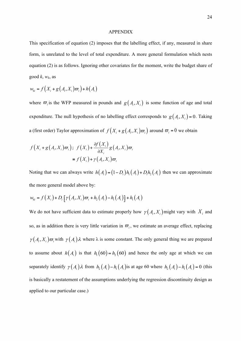
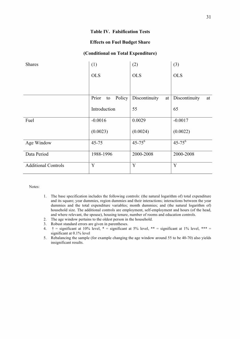