ORNL/TM-2012/592

Case Study of the Maplewood Park Multifamily Retrofit for Energy Efficiency

December 2012 Prepared by Piljae Im, Ph.D. Eyu-Jin Kim Mini Malhotra, Ph.D. Robert Stephenson Sydney Roberts, Ph.D.

DOCUMENT AVAILABILITY Reports produced after January 1, 1996, are generally available free via the U.S. Department of Energy (DOE) Information Bridge. Web site http://www.osti.gov/bridge Reports produced before January 1, 1996, may be purchased by members of the public from the following source. National Technical Information Service 5285 Port Royal Road Springfield, VA 22161 Telephone 703-605-6000 (1-800-553-6847) TDD 703-487-4639 Fax 703-605-6900 E-mail info@ntis.gov Web site http://www.ntis.gov/support/ordernowabout.htm Reports are available to DOE employees, DOE contractors, Energy Technology Data Exchange (ETDE) representatives, and International Nuclear Information System (INIS) representatives from the following source. Office of Scientific and Technical Information P.O. Box 62 Oak Ridge, TN 37831 Telephone 865-576-8401 Fax 865-576-5728 E-mail reports@osti.gov Web site http://www.osti.gov/contact.html

This report was prepared as an account of work sponsored by an agency of the United States Government. Neither the United States Government nor any agency thereof, nor any of their employees, makes any warranty, express or implied, or assumes any legal liability or responsibility for the accuracy, completeness, or usefulness of any information, apparatus, product, or process disclosed, or represents that its use would not infringe privately owned rights. Reference herein to any specific commercial product, process, or service by trade name, trademark, manufacturer, or otherwise, does not necessarily constitute or imply its endorsement, recommendation, or favoring by the United States Government or any agency thereof. The views and opinions of authors expressed herein do not necessarily state or reflect those of the United States Government or any agency thereof.

ORNL/TM-2012/592

Energy and Transportation Science Division

CASE STUDY OF THE MAPLEWOOD PARK MULTIFAMILY RETROFIT FOR ENERGY EFFICIENCY

Eyu-Jin Kim Robert Stephenson

Sydney Roberts, Ph.D.

SOUTHFACE ENERGY INSTITUTE 241 Pine Street NE, Atlanta, Georgia 30308

Piljae Im, Ph.D.

Mini Malhotra, Ph.D.

OAK RIDGE NATIONAL LABORATORY Oak Ridge, Tennessee 37831-6283

managed by UT-BATTELLE, LLC

Date Published: December 2012

Prepared for

Building Technologies Program US Department of Energy

iii

CONTENTS

Page

LIST OF FIGURES ................................................................................................................................. v LIST OF TABLES ................................................................................................................................ vii ABBREVIATIONS, ACRONYMS, AND INITIALISMS ...................................................................... ix EXECUTIVE SUMMARY .................................................................................................................... xi 1. INTRODUCTION ........................................................................................................................... 1

1.1 OVERVIEW .......................................................................................................................... 1 1.2 FUNDING PROCESS ............................................................................................................ 2 1.3 CONSTRUCTION SCHEDULE ............................................................................................ 3 1.4 DEFINING THE BUILDING ENVELOPE ............................................................................ 3 1.5 PRE- AND POST-RETROFIT BUILDING CHARACTERISTICS ........................................ 5

1.5.1 Walls ......................................................................................................................... 5 1.5.2 Windows and Exterior Doors ..................................................................................... 6 1.5.3 Roof and Ceiling........................................................................................................ 6 1.5.4 Foundation ................................................................................................................ 6 1.5.5 Heating, Ventilation, and Air Conditioning System .................................................... 7 1.5.6 Domestic Water Heater .............................................................................................. 8 1.5.7 Plumbing ................................................................................................................... 9 1.5.8 Lighting ..................................................................................................................... 9 1.5.9 Appliances ............................................................................................................... 10 1.5.10 Other ....................................................................................................................... 10

1.6 COST OF RETROFIT MEASURES .................................................................................... 11 2. DUCT AND ENVELOPE LEAKAGE TESTING.......................................................................... 12

2.1 STANDARD PROGRAMMATIC TESTS IN SAMPLE UNITS .......................................... 12 2.1.1 Duct Leakage Test ................................................................................................... 12 2.1.2 Single Point Envelope Leakage Test ........................................................................ 12 2.1.3 Test Results ............................................................................................................. 13

2.2 DETAILED INFILTRATION TESTS IN BUILDING #7 ..................................................... 13 2.2.1 Guarded Multipoint Infiltration Test ........................................................................ 14 2.2.2 Unguarded and Guarded Single Point Infiltration Test.............................................. 16

3. ENERGY ANALYSIS .................................................................................................................. 17 3.1 WHOLE-BUILDING ENERGY ANALYSIS OF A REPRESENTATIVE BUILDING ........ 17

3.1.1 Weather Normalization of Billed Energy Use ........................................................... 17 3.1.2 Calibration of Building Energy Model ..................................................................... 20 3.1.3 Analysis of Energy Efficiency Measures .................................................................. 22

3.2 ENERGY ANALYSIS OF SAMPLE UNITS ....................................................................... 23 4. SUMMARY AND CONCLUSION ............................................................................................... 25

4.1 OPPORTUNITIES ............................................................................................................... 25 4.2 CHALLENGES ................................................................................................................... 26 4.3 MISSED OPPORTUNITIES ................................................................................................ 27

REFERENCES ..................................................................................................................................... 29 APPENDIX A. MAPLEWOOD ARCHITECTURAL PLANS ............................................................ A-1 APPENDIX B. MAPLEWOOD PHOTOGRAPHS .............................................................................. B-1 APPENDIX C. MAPLEWOOD QAP SUSTAINABILITY CHECKLIST ........................................... C-1 APPENDIX D. DIAGNOSTIC TEST DATA FOR SAMPLE UNITS ................................................. D-1 APPENDIX E. CALIBRATION RESULTS .........................................................................................E-1 APPENDIX F. CONSIDERATIONS FOR WHOLE-BUILDING ENERGY ANALYSIS .................... F-1

iv

APPENDIX G. ASHRAE STANDARD 62.2 COMPLIANCE CHECK ............................................... G-1 APPENDIX H: ENERGY EFFICIENCY MEASURES DESCRIPTION AND COST DATA .............. H.1 APPENDIX I. REM/RATETM RESULTS FOR ENERGY ANALYSIS OF SAMPLE UNITS ............... I-1

v

LIST OF FIGURES Figure Page

Fig. 1. Aerial view of Maplewood Park Apartments. ................................................................................ 1 Fig. 2. View of Building #7 in Maplewood Park Apartments. .................................................................. 2 Fig. 3. LIHTC funding process. ............................................................................................................... 2 Fig. 4. 3D rendering of buildings ............................................................................................................. 4 Fig. 5. New fiber cement siding. .............................................................................................................. 5 Fig. 6. New double-pane, low-e, vinyl-frame windows. ........................................................................... 6 Fig. 7. Existing R-30 insulation in the attic. ............................................................................................. 6 Fig. 8. Attic insulation upgraded to R-38. ................................................................................................ 6 Fig. 9. Existing insulation and vapor barrier in the crawlspace. ................................................................ 7 Fig. 10. New insulation and vapor barrier in the crawlspace ..................................................................... 7 Fig. 11. Existing indoor unit the air handler. ............................................................................................ 8 Fig. 12. New outdoor units of the heat pump. ........................................................................................... 8 Fig. 13. Existing domestic water heater. ................................................................................................... 8 Fig. 14. New domestic water heater. ........................................................................................................ 8 Fig. 15. Existing plumbing fixtures .......................................................................................................... 9 Fig. 16. New plumbing fixtures ............................................................................................................... 9 Fig. 17. Existing incandescent lamp in a recessed lighting fixture. ........................................................... 9 Fig. 18. New CFLs in a bathroom vanity fixture. ..................................................................................... 9 Fig. 19. Existing kitchen appliances ....................................................................................................... 10 Fig. 20. New kitchen appliances ............................................................................................................ 10 Fig. 21. Pre-retrofit service penetrations through walls and ceiling. ........................................................ 10 Fig. 22. Duct leakage testing setup showing revised methodology. ......................................................... 12 Fig. 23. Blower door setup. .................................................................................................................... 12 Fig. 24. Statistics of pre and post-retrofit envelope and duct leakage based on the sample units. ............. 13 Fig. 25. Multifan set-up using TECLOG2 software. ............................................................................... 14 Fig. 26. Regression model for pre- and post-retrofit multipoint blower door test..................................... 15 Fig. 27. Cluster column plot of billed energy use. .................................................................................. 18 Fig. 28. Determination of billing period start and end dates. ................................................................... 19 Fig. 29. Regression model for billed energy use. .................................................................................... 19 Fig. 30. Calibrated simulation model compared with billed energy use data. .......................................... 20 Fig. 31. Annual energy use for all EEMs................................................................................................ 23 Fig. 32. Pre and post-retrofit site energy consumption for the sample units. ............................................ 24

vii

LIST OF TABLES Table Page

Table ES- 1. Summary of energy and economic analysis for EEMs ........................................................ xii Table 1. Economics of the project ............................................................................................................ 3 Table 2. Construction schedule ................................................................................................................ 3 Table 3. Details of Maplewood units........................................................................................................ 5 Table 4. Manual J load calculations ......................................................................................................... 7 Table 5. Installed cost of retrofit measures ............................................................................................. 11 Table 6. Pre- and post-retrofit multipoint blower door test results .......................................................... 16 Table 7. Pre-retrofit single point unguarded and guarded blower door test results ................................... 16 Table 8. Billed energy use for Building #7 ............................................................................................. 17 Table 9. Baseline characteristics ............................................................................................................ 20 Table 10. Results of energy and economic analysis of EEMs ................................................................. 22

ix

ABBREVIATIONS, ACRONYMS, AND INITIALISMS 3-D three-dimensional

ACE Protocol Army Corps of Engineers Air Leakage Test Protocol for Building Envelopes

ACH air change per hour

ACH50 Number of complete air changes that will occur in 1 hour with 50 Pascal of pressure applied uniformly across the building envelope

CDD cooling degree days (amount of energy used to cool a building, using 70° as a baseline)

CFL compact fluorescent lamp

CFM cubic feet per minute

CFM25 Air flow (CFM) at 25 Pascal (duct leakage measurement)

CFM50 Air flow (CFM) at 50 Pascal (infiltration measurement)

CVRMSE coefficient of variation root mean squared error

DCA The Georgia Department of Community Affairs

DHW domestic hot water

dwelling unit A single unit providing complete independent living facilities for one or more persons, including permanent provisions for living, sleeping, eating, cooking and sanitation

EEM energy efficiency measure

EF energy factor, domestic water heating

ELA elective leakage area

gpf gallons per flush

gpm gallons per minute

HDD heating degree days ( measure of energy used to heat a building, using 65° as a baseline)

HERS Home Energy Rating System

HSPF Heating Seasonal Performance Factor (heating efficiency)

HUD US Department of Housing and Urban Development

HVAC heating, ventilation, and air-conditioning

IECC International Energy Conservation Code

IMT Inverse Modeling Toolkit

LIHTC Low-Income Housing Tax Credit

MMBtu million British thermal units

x

QAP Qualified Allocation Plan

RESNET Residential Energy Services Network

SEER Seasonal Energy Efficiency Ratio (cooling efficiency)

SHGC Solar Heat Gain Coefficient

TMY Typical metrological year

VOC volatile organic compound

xi

EXECUTIVE SUMMARY Maplewood Park (Maplewood), a 110-unit multifamily apartment complex in Union City, Georgia, completed major renovations under the guidance of a third-party green building certification program in October 2012. Oak Ridge National Laboratory (ORNL) partnered with Southface Energy Institute (Southface) to use this project as a case study of energy retrofits in low-rise, garden-style, multifamily buildings in the southeastern United States. This report provides a comprehensive profile of this project including the project economics, findings of the building audit, and results of the analysis of energy retrofit measures specific to this project. With a main focus of energy retrofits, this report aims to discuss other aspects of multifamily building retrofit that would benefit future projects in terms of improved building audit process, streamlined tasks, and higher energy savings in low-rise, garden-style apartments.

Maplewood received Low Income Housing Tax Credit (LIHTC) financing via the 2010 Georgia Qualified Allocation Plan (QAP). To be eligible for QAP funds in Georgia, all major renovations must incorporate energy-efficiency measures and adopt a third-party green building certification. Because of the unique demands of this financing, including requirements for long-term ownership, property owners were also especially motivated to invest in upgrades that will increase durability and comfort while reducing the energy cost for the tenants.

The renovation of the eleven buildings of Maplewood was completed in six phases, with two buildings audited and renovated in each of the first five phases. The building audit included visual assessment of the building and diagnostic testing of a sample of unit to determine the existing conditions and potential improvements. Pre- and post-retrofit blower door and duct blaster testing were conducted on the sample units to determine the envelope and duct leakage and effectiveness of air sealing. An additional test with multiple blower doors was conducted on a representative building before and after the retrofits to quantify the air leakage to the outdoors and to the adjacent units.

The Maplewood project team exercised a whole-building approach to meet or exceed 2009 International Energy Conservation Code (IECC) by upgrading to a tighter and better insulated building envelope and replacing windows, doors, lighting, appliances, and HVAC and DHW systems with Energy Star® qualified products. In addition, other retrofit measures were implemented to improve the appearance and durability of the buildings.

Southface performed pre- and post-retrofit energy analysis of the sample units using REM/RateTM

software and generated Home Energy Rating Score (HERS) index for the units. The analysis showed an average HERS index of 107 before the retrofits and 87 after the retrofits, and an average of 20% reduction in annual energy use from the selected energy-efficiency measures.

ORNL conducted a whole-building energy analysis of a representative building in Maplewood using MulTEA (Multfamily Tool for Energy Audit) to predict post-retrofit energy savings and identify alternative potential energy savings measures. The building energy model was first calibrated using the pre-retrofit utility bills. Using this model, the analysis was conducted for the measures implemented on the building as well as some additional measures.

Table ES-1 summarizes the results of whole-building energy analysis. Among the eight measures (EEM 1 through 8) implemented in the building, window replacement shows as the most cost effective measure, followed by heat pump replacement and water heater replacement. Lighting replacement resulted in 4% energy savings but had 12 year payback period due to the cost of fixture replacement included in the measure cost. On the other hand, increasing attic insulation from R-30 to R-38 and kitchen appliance

xii

replacement showed as the least cost effective measures with very small energy savings and 60-70 year payback period.

Six additional measures were considered for the analysis (EEM 9 through 14), which included insulating crawlspace walls, installing exterior insulation on exterior walls (since the wall siding replacement was considered for appearance and durability), installing window film, installing storm windows, and installing programmable thermostat. Among these, installing storm windows was the most cost effective measure with 3.6% energy savings and 5.4 year payback period, whereas installing window film resulted in very small savings. Other measures showed about 2% savings with 6-13 year payback period.

The analysis projected a 25% energy savings from the measures installed in the building with a payback period of 10 years. The analysis also indicated that, with a careful selection of measures, up to 38% energy savings could be achieved with a payback period of less than 6 years.

Table ES- 1. Summary of energy and economic analysis for EEMs

EEM Energy

savings (%) Cost of measure for

Building #7 ($) Payback

(year) 1 Insulate crawlspace ceiling with R-19 batt insulation 1.7% $300 1.1 2 Increase attic insulation from R-30 to R-38 0.1% $1,205 61.5 3 Replace windows and doors 9.4% $5,850 3.9 4 Replace 12 SEER, 7.5 HSPF heat pump with 14 SEER, 8.3/8.5 HSPF unit 7.2% $5,871 5.1 5 Replace incandescent lamps and fixtures with CFLs 4.1% $7,851 12.1 6 Replace kitchen appliances 1.0% $10,544 68.7 7 Replace 0.9 EF water heater with 0.93 EF unit 2.7% $3,012 6.9 8 Air seal building to reduce air infiltration by 25% 2.1% $4,758 14.0 9 Air seal crawlspace and insulate crawlspace walls with R-5 rigid insulation 1.8% $3,809 13.1 10 Air seal crawlspace and insulate crawlspace walls with R-13 batt insulation 2.1% $3,134 9.2 11 Install R-5 rigid insulation on exterior walls 2.1% $3,371 10.0 12 Install window film 0.4% $1,106 16.5 13 Install storm windows 3.6% $3,080 5.4 14 Install programmable thermostat 1.7% $1,700 6.2

Implemented EEMs package (1 through 8) 25.1% $39,390 9.8 Cost-optimized EEMs package (EEM 1, 3, 4, 5, 7, 8, 11, and 14) 37.9% $32,713 5.4

It is hoped that this study will also provide insight for the development of suitable and accessible audit tools and protocols that can be applied to other multifamily building types such as Maplewood.

Multifamily building retrofit presents challenges because, unlike in single-family audits, multiple players are involved—building owner, developer, contractor, architect, consultants, and tenants. Coordinating all involved parties requires extensive planning and execution, resulting in less flexibility.

1

1. INTRODUCTION This case study focuses on the renovation of Maplewood Park Apartments (Maplewood), a multifamily apartment complex in Union City, Georgia – a suburb, 18 miles southwest from Atlanta, Georgia. Maplewood provides low-income rental housing to families and senior citizens. The renovation included energy upgrades such as air sealing, window and door replacement, replacement of heating, ventilation, and air-conditioning (HVAC) and domestic hot water (DHW) systems, lighting, and appliances, as well as other upgrades such as roofing and wall siding replacement. The energy upgrades selected to bring the buildings up to the current Georgia Code (i.e., 2009 International Energy Conservation Code (IECC)) are estimated to achieve 25% annual energy savings.

The federal Low Income Housing Tax Credit (LIHTC) provided funding for the project, which drove the decision process for the measures implemented into the renovation and mandated participation in a third-party green building certification program. This federal subsidy finances the development of low-income rental housing across the United States. Local housing and community development agencies, in this case the Georgia Department of Community Affairs (DCA), disburse the funds through a competitive process that provides incentives for projects to include features that improve energy efficiency. The specifics of this funding mechanism are covered in a subsequent section.

1.1 OVERVIEW

Built in 1993, Maplewood is an apartment complex with 11 buildings, each consisting of 10 units. Fig. 1 shows an aerial view of Maplewood with the building numbers shown on the buildings. Fig. 2 shows a view of Building #7 in Maplewood before renovation. The buildings underwent minor renovations in 2008, during which HVAC systems, appliances, and/or domestic water heater in some units were replaced due to specific system failures.

Fig. 1. Aerial view of Maplewood Park Apartments. (Photo courtesy Google® Earth)

2

Fig. 2. View of Building #7 in Maplewood Park Apartments.

1.2 FUNDING PROCESS

Low-income subsidies through LIHTC (HUD 2010) funded the renovation of Maplewood. LIHTC encourages building owners and developers to undertake the renovation of existing low-income multifamily housing. Fig. 3 shows the funding process of LIHTC. The US Department of Housing and Urban Development (HUD) oversees the program and distributes tax credit funding to individual states based on demonstrated need. The designated agency for each state (e.g., the Georgia DCA) has a Qualified Allocation Plan (QAP) (e.g., GDCA 2010) that outlines the competitive process by which tax credits are awarded to individual projects. The QAP considerations are updated annually and new candidates are encouraged to apply in every cycle. Once a project has been selected for an award, the developer can hold the tax credit to offset the tax liability. However, typically, the developer sells the tax credits in the open market to an investor or syndicator to raise funds for the project in order to reduce the equity or debt financing required for the project. This allows the developer to provide affordable housing at reduced rental rates.

During the 2010 QAP cycle, 30 projects were accepted including Maplewood. Maplewood had a financial package typical of many affordable housing projects, combining affordable housing subsidies (such as LIHTC) and private equity funding. Table 1 shows the economics of the project including the sources of funds and allocation of those funds. The project received $10.6 million, which included $6.65 million (63%) from LIHTC and $3.37 million (32%) as mortgage1. Of the available funds, $3.9 million (37%) was allocated as hard construction costs, and $0.6 million (5.7%) was allocated as soft costs2 to cover expenditure for programs, project management, administration, and marketing.

1 The annual mortgage rate was not public. 2 The soft costs included $8,500 for the third-party green building certification and $15,000 for participating in a local utility’s rebate/incentive program. The latter would provide the building owner $90,450 in rebates.

Fig. 3. LIHTC funding process.

Courtesy Kim et al. (2012)

Federal GovernmentU.S. Department of Housing

and Urban Development

State GovernmentGeorgia Department of

Community Affairs

Affordable Housing ProjectMaplewood Park

Apartments

Investor or Syndicator

3

Table 1. Economics of the project

Source of funds Amount ($) Percent

First mortgage 3,370,000 31.9%

Low income tax credits 6,654,984 62.9%

Tax credit assistance program 0 0.0%

Owner equity 0 0.0%

Deferred developer fee 550,964 5.2%

Total 10,575,948

Allocation of funds Amount ($) Percent

Land acquisition and buildings 3,200,000 30.3%

Hard construction costs 3,900,445 36.9%

Contingency 390,045 3.7%

Soft costs 597,813 5.7%

Cost of issuance/financing fees 70,800 0.7%

Capitalized interest 71,486 0.7%

Startup and reserves 739,192 7.0%

Relocation 141,670 1.3%

Equity costs 130,939 1.2%

Developer fees 1,333,558 12.6%

Total 10,575,948

1.3 CONSTRUCTION SCHEDULE

The renovation of Maplewood was scheduled to progress in six phases (Table 2). Phase I through V incorporated renovation of two buildings, each. Phase VI incorporated renovation of one building. Building audits were also conducted in phases based on the construction schedule. Pre-renovation assessments for the project began in December 2011. Assessors visited the site and performed a detailed inspection of the buildings and a sample set of units. The tenants were relocated before each phase began and allowed to return after the renovation was completed. The construction completed in October 2012.

As part of the property assessment, the existing conditions of the buildings and sample units were documented in each phase to establish a baseline for the property’s energy profile and other performance aspects, such as water use and durability. The potential improvements to the whole-building performance were examined by focusing on upgrades to the building envelope, HVAC system, DHW system, lighting, and appliances. In addition to energy savings, the project team considered cost and constructability before arriving at the final design specifications for the renovation. Inspections were also conducted after retrofits in each building to document the final upgraded conditions.

1.4 DEFINING THE BUILDING ENVELOPE

Due to the sloping site, the three-story buildings of Maplewood have foundation on two levels – a slab-on-grade floor towards the lower grade and vented crawlspace towards the higher grade. The units on the lowest floor (terrace level) have one wall abutting the crawlspace. The units on the upper floors have one party wall. Fig. 4 shows a three-dimensional (3D) rendering of the buildings. Three unit types were found across the 11 buildings of Maplewood: A, B, and C. Fig. 4 indicates the unit types found in the buildings. Table 3 provides an overview of characteristics of each unit type and their distribution across Maplewood. Appendix A includes the architectural plan of the three unit types. Each unit has an exterior entrance door opening to a breezeway located in the center of the building along the east-west axis. This arrangement

Table 2. Construction schedule

Phase Buildings Completion month and

year I 5, 9 December 2011 II 4, 10 February 2012 III 6, 11 April 2012 IV 3, 7 May 2012 V 2, 8 October 2012 VI 1 October 2012

4

divides each building into two detached wings: wing one to the south and wing two to the north. A firewall runs up to the roofline, separating the vented attic above each wing. In collecting a unit’s dimensions, RESNET protocols on measuring takeoffs of building components (RESNET 2012) were followed.

(a) Building 1 (unit A)

(b) Buildings 3-6 (units B and C)

(c) Buildings 2, 7-11 (units A and C)

Fig. 4. 3D rendering of buildings

A

C

C

B

A

A Party walls between adjacent units

Wall exposed to the vented crawlspace

5

Table 3. Details of Maplewood units

Unit type Description Conditioned

floor area (ft2)

Number of units (by unit type) per building Total number of units Building 1 Building 3-6 Building 2, 7-11

A Two bedrooms, two bath 1,049 10 - 6 46 B Three bedroom, two bath 1,176 - 6 - 24 C Three bedroom, two bath 1,260 - 4 4 40

Total 126,878 110

1.5 PRE- AND POST-RETROFIT BUILDING CHARACTERISTICS

Projects submitted under QAP cycle must earn a minimum of 10 out of 40 points in at least 4 out of 7 categories, which include energy efficient building envelope, lighting, water conservation, indoor air quality, resource efficiency, education, and innovation (see Appendix C for details of the project score card), while meeting or exceeding the following criteria:

• Compliance with applicable Georgia Energy Code (i.e., 2009 IECC) • Minimum HVAC system efficiency based on the weather location • Minimum domestic water heater efficiency (i.e., 0.62 EF for gas and 0.93 EF for electric water heater) • Energy Star appliances including refrigerators, dishwashers, and clothes washers3

Therefore, as part of the renovation, an energy upgrade package for the project was chosen to meet or exceed the State of Georgia 2010 QAP requirements for energy efficiency. The following sections describe the pre and post-retrofit building characteristics. Table 5 summarizes the specification and cost of energy retrofits. Appendix B includes additional photos taken during the pre- and post-renovation visits.

1.5.1 Walls

The walls of the units were constructed of 2×4 wood frame @16 in. o.c. The insulation in the wall cavities were determined to be R-13 fiberglass batt in the exterior walls and R-11 fiberglass batt in party wall. The existing exterior wall finish included a combination of vinyl siding and brick veneer.

The vinyl siding was replaced with fiber cement siding and brick veneer was replaced with new brick fascia (Fig. 5). No other changes were made to the walls.

3 Clothes washers were not considered in this project because the units did not have pre-installed laundry equipment.

Fig. 5. New fiber cement siding.

6

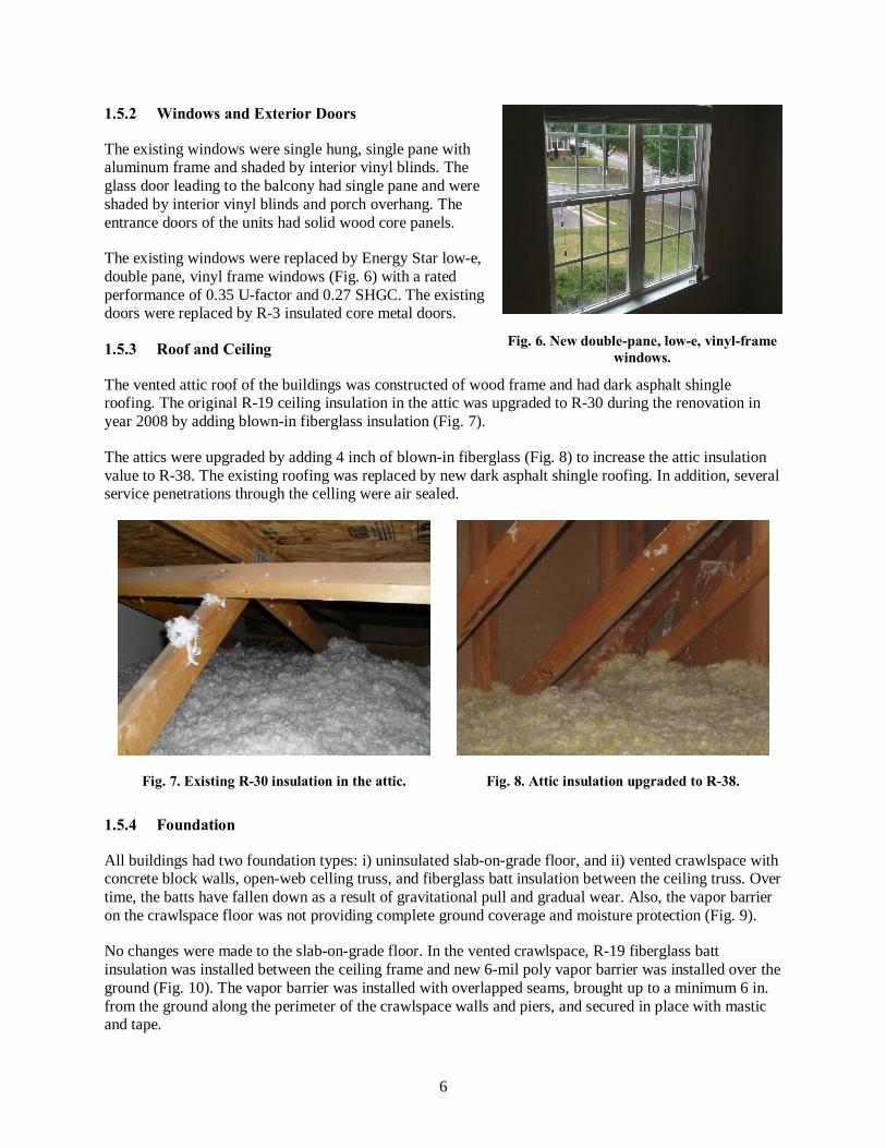
1.5.2 Windows and Exterior Doors

The existing windows were single hung, single pane with aluminum frame and shaded by interior vinyl blinds. The glass door leading to the balcony had single pane and were shaded by interior vinyl blinds and porch overhang. The entrance doors of the units had solid wood core panels.

The existing windows were replaced by Energy Star low-e, double pane, vinyl frame windows (Fig. 6) with a rated performance of 0.35 U-factor and 0.27 SHGC. The existing doors were replaced by R-3 insulated core metal doors.

1.5.3 Roof and Ceiling

The vented attic roof of the buildings was constructed of wood frame and had dark asphalt shingle roofing. The original R-19 ceiling insulation in the attic was upgraded to R-30 during the renovation in year 2008 by adding blown-in fiberglass insulation (Fig. 7).

The attics were upgraded by adding 4 inch of blown-in fiberglass (Fig. 8) to increase the attic insulation value to R-38. The existing roofing was replaced by new dark asphalt shingle roofing. In addition, several service penetrations through the celling were air sealed.

Fig. 7. Existing R-30 insulation in the attic. Fig. 8. Attic insulation upgraded to R-38.

1.5.4 Foundation

All buildings had two foundation types: i) uninsulated slab-on-grade floor, and ii) vented crawlspace with concrete block walls, open-web celling truss, and fiberglass batt insulation between the ceiling truss. Over time, the batts have fallen down as a result of gravitational pull and gradual wear. Also, the vapor barrier on the crawlspace floor was not providing complete ground coverage and moisture protection (Fig. 9).

No changes were made to the slab-on-grade floor. In the vented crawlspace, R-19 fiberglass batt insulation was installed between the ceiling frame and new 6-mil poly vapor barrier was installed over the ground (Fig. 10). The vapor barrier was installed with overlapped seams, brought up to a minimum 6 in. from the ground along the perimeter of the crawlspace walls and piers, and secured in place with mastic and tape.

Fig. 6. New double-pane, low-e, vinyl-frame windows.

7

Fig. 9. Existing insulation and vapor barrier in the crawlspace.

Fig. 10. New insulation and vapor barrier in the crawlspace

1.5.5 Heating, Ventilation, and Air Conditioning System

Each unit had a dedicated central heat pump system with a rated performance of 12 SEER and 7.5 HSPF4. The two-bedroom units (Unit A) were served by 1.5 ton systems and the three-bedroom units (Unit B and C) were served by 2 ton systems. The air handler was located in a louvered closet in either a bathroom (Unit A), the utility room (Unit B), or a bedroom (Unit C) (Fig. 11). Ducts were located in the conditioned space within the dropped soffit. Outdoor condenser unit was installed on a concrete pad at the sides of the building.

The existing heat pump systems were replaced with Energy Star qualified heat pump systems (Fig. 12). Manual-J load calculations were performed for equipment sizing (Table 4). However, the systems selected for the replacement were of the same size as existing systems, which were about 1.5 times oversized. The two-bedroom unit (Unit A) were installed with 1.5 ton systems with a rated performance of 14.5 SEER and 8.3 HSPF. The three-bedroom units (Units B and C) were installed with 2 ton systems with a rated performance of 14.5 SEER and 8.5 HSPF. The inspection report notes that mastic was applied along the seams and joint connections of the ductwork in the air handler. No air sealing was performed for the ducts that were within the dropped soffits.

The existing ceiling-mounted exhaust fans in the bathrooms were replaced with new exhaust fans and connected to the existing exhaust ducts vented to the outside. The existing recirculating range hoods were replaced by new recirculating range hoods.

4 During the 2008 renovation, some of the outdoor units were upgraded for maintenance need and system failures.

Table 4. Manual J load calculations

Unit type Cooling load (kBtu/h)

Heating load (kBtu/h)

A 11.9 12.8

B 14.9 16.7

C 15.1 16.3

Reinstalled R-19 fiberglass batt

Deteriorated vapor

Deteriorated insulation

New 6 mil poly vapor barrier

8

Fig. 11. Existing indoor unit the air handler. Fig. 12. New outdoor units of the heat pump.

1.5.6 Domestic Water Heater

All units were equipped with a 40-gal, lowboy electric water heater with a rated performance of 0.90 EF. Some of the inspected water heaters had insulation blankets5. All inspected water heaters were in poor condition with signs of corrosion (Fig. 13). All existing water heaters were replaced with new 40-gal electric water heaters with a rated performance of 0.93 EF (Fig. 14).

Fig. 13. Existing domestic water heater. Fig. 14. New domestic water heater.

5 The effective average R-value for the insulation blankets was modeled as R-3 in REM/RateTM.

Deteriorated insulation blanket

9

1.5.7 Plumbing

The existing plumbing fixtures in the units included 2 gpm faucets (Fig. 15), 1.6 gpf toilets, and 5.0 gpm showerheads, which were replaced by low-flow plumbing fixtures including 1.5 gpm faucets (Fig. 16), 1.28 gpf toilets, and 1.5 gpm showerheads.

Fig. 15. Existing plumbing fixtures Fig. 16. New plumbing fixtures

1.5.8 Lighting

The existing lighting included 18-60W incandescent lamps in two bedroom units (Unit A), 21-60W incandescent lamps in three bedroom units (Units B and C) (Fig. 17), and two T12 lamps and a small 15W pin-base tube in the kitchen in all units. The lighting was upgraded to a 100% Energy Star lighting package, which included replacing the existing T12 lamps with new T12 lamps and replacing all incandescent lamps with 13W CFLs (Fig. 18).

Fig. 17. Existing incandescent lamp in a recessed lighting fixture.

Fig. 18. New CFLs in a bathroom vanity fixture.

10

1.5.9 Appliances

The existing appliances in a unit included a refrigerator, a dishwasher, and an electric range (Fig. 19). The appliances were from various manufacturers with unknown wattage. These appliances were replaced with Energy Star qualified 18 ft3 refrigerator (388 kWh/year rated energy use) and dishwasher (306 kWh/year rated energy use), and an electric range with two 6 in. (1500 W) and two 8 in. (2600 W) high-speed coil elements (Fig. 20).

The unit had connections for clothes washer and dryer for optional installation of these appliances by occupants. However, at the time of the audits, the units were unoccupied with no evidence of the use of laundry equipment during occupancy.

Fig. 19. Existing kitchen appliances Fig. 20. New kitchen appliances

1.5.10 Other

Gaps were found around service penetrations through the walls and ceiling of the units (Fig. 21). Air sealing was performed to fill these gaps. In all units, the floor tiles and carpet were replaced and interior surfaces were repainted with low-VOC paints.

Fig. 21. Pre-retrofit service penetrations through walls and ceiling.

11

1.6 COST OF RETROFIT MEASURES

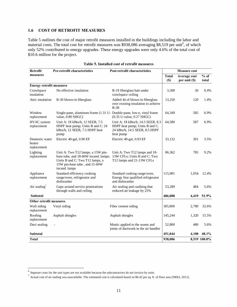
Table 5 outlines the cost of major retrofit measures installed in the buildings including the labor and material costs. The total cost for retrofit measures was $938,086 averaging $8,519 per unit6, of which only 52% contributed to energy upgrades. These energy upgrades were only 4.6% of the total cost of $10.6 million for the project.

Table 5. Installed cost of retrofit measures

Retrofit measures

Pre-retrofit characteristics Post-retrofit characteristics Measure cost Total

($) Average cost per unit ($)

% of total

Energy retrofit measures Crawlspace insulation

No effective insulation R-19 fiberglass batt under crawlspace ceiling

3,300 30 0.4%

Attic insulation R-30 blown-in fiberglass Added 4” of blown-in fiberglass over existing insulation to achieve R-38

13,250 120 1.4%

Window replacement

Single-pane, aluminum frame (1.31 U-value, 0.80 SHGC)

Double-pane, low-e, vinyl frame (0.35 U-value, 0.27 SHGC)

64,349 585 6.9%

HVAC system replacement

Unit A: 18 kBtu/h, 12 SEER, 7.5 HSPF heat pump; Units B and C: 24 kBtu/h, 12 SEER, 7.5 HSPF heat pump

Unit A: 18 kBtu/h, 14.5 SEER, 8.3 HSPF heat pump; Units B and C: 24 kBtu/h, 14.5 SEER, 8.5 HSPF heat pump

64,580 587 6.9%

Domestic water heater replacement

Electric 40-gal, 0.90 EF Electric 40-gal, 0.93 EF 33,132 301 3.5%

Lighting replacement

Unit A: Two T12 lamps, a 15W pin-base tube, and 18-60W incand. lamps; Units B and C: Two T12 lamps, a 15W pin-base tube , and 21-60W incand. lamps

Unit A: Two T12 lamps and 18-13W CFLs; Units B and C: Two T12 lamps and 21-13W CFLs

86,362 785 9.2%

Appliance replacement

Standard efficiency cooking range/oven, refrigerator and dishwasher

Standard cooking range/oven, Energy Star qualified refrigerator and dishwasher

115,981 1,054 12.4%

Air sealing7 Gaps around service penetrations through walls and ceiling

Air sealing and caulking that reduced air leakage by 25%

53,289 484 5.6%

Subtotal 486,088 4,419 51.9% Other retrofit measures Wall siding replacement

Vinyl siding Fiber cement siding 305,800 2,780 32.6%

Roofing replacement

Asphalt shingles Asphalt shingles 145,244 1,320 15.5%

Duct sealing - Mastic applied to the seams and joints of ductwork in the air handler

52,800 480 5.6%

Subtotal 451,044 4,100 48.1% Total 938,086 8,519 100.0%

6 Separate costs for the unit types are not available because the subcontractors do not invoice by units. 7 Actual cost of air sealing was unavailable. The estimated cost is calculated based on $0.42 per sq. ft. of floor area (NREL 2012).

12

2. DUCT AND ENVELOPE LEAKAGE TESTING Two testing approaches were executed for this project: standard programmatic tests in the sample units to determine the duct leakage and envelope leakage, and detailed envelope leakage tests in Building #7 to determine the air leakage to the outdoors and between adjacent units of the building. The tests were performed under the guidance of the RESNET standards (RESNET 2011). The envelope leakage test was performed by depressurizing each unit to 50 Pa and measuring the airflow in cubic feet per minute (CFM50) passing through the blower door fan. The duct leakage-to-outside test was performed by pressurizing the unit to 25 Pa and then the duct system to 25 Pa, measuring the airflow (CFM25) passing through the fan. Of particular interest for researchers was determining the air leakage between adjacent units that occurs across the partition walls and ceiling/floor.

2.1 STANDARD PROGRAMMATIC TESTS IN SAMPLE UNITS

2.1.1 Duct Leakage Test

Using a Duct Blaster kit, duct leakage test was performed in sample units before and after retrofit. The HVAC system air handler was located in mechanical closets with an open return with a filter attached. There was not adequate space in the closet to place the kit at the return plenum because the lowboy water heater was located under the air handler (Fig. 26a). Therefore, a workaround had to be improvised for the standard RESNET protocols, which state that the duct leakage testing system be attached to the largest return grille closest to the air handler. As a work around, the filter was taken out and the return was sealed with duct tape. Figure 26a shows the location where the duct mask was placed (duct mask is not shown). The supply closest to the plenum was pressurized (as shown in Fig. 26b), with the reference hose leading to another return. The duct leakage-to-outside test was performed by pressurizing the building unit to 25 Pa and then pressurizing the duct system to 25 Pa, measuring the air flow at 25 Pa (CFM25) through the fan.

2.1.2 Single Point Envelope Leakage Test

A single point infiltration test measures the air leakage of a unit at a single reference pressure using a blower door fan (Fig. 23). The testing procedures followed RESNET (2011), starting with preparing the building enclosure for testing by closing and latching all exterior doors and windows, opening all interior doors, and shutting down all HVAC and ventilation fans. During the single point test, adjacent units were left in their natural state with no induced pressures or opened windows.

Fig. 22. Duct leakage testing setup showing revised methodology. Fig. 23. Blower door setup.

(a)

Return Plenum

Water Heater

(b) Supply Grill

Mechanical Closet

13

2.1.3 Test Results

The statistics of the envelope and duct leakage based on the 21 sample units are shown in Fig. 24. The test results are shown in Appendix F. After renovations were completed, envelope leakage for most of the units was reduced to meet the IECC 2009 maximum acceptable infiltration threshold of 7 ACH50.

Considering that the ducts were in the conditioned space inside the thermal and pressure boundary of the building, the reason for duct leakage to the outside was undetermined and remained a subject for investigation in future multifamily research.

Fig. 24. Statistics of pre and post-retrofit envelope and duct leakage based on the sample units.

2.2 DETAILED INFILTRATION TESTS IN BUILDING #7

This experiment was conducted to provide results from guarded testing, an alternate infiltration testing method. Guarded tests of multifamily units can isolate leakage to the outdoors from leakage to adjacent units. The additional data and insight gathered from guarded testing require add to the cost and complexity given that additional personnel, equipment, and setup time are required. Two guarded test approaches were performed using multiple blower doors and the Energy Conservatory’s TECLOG2 data logging software that provides simultaneous control of multiple blower door systems. Testing standards and protocols were followed using RESNET (2011), ACE (2012), and ASTM (1999). These tests were conducted on all ten units in Building #7 before and after retrofit.

A guarded test measures unit air leakage at a reference pressure while inducing the same reference pressure to adjacent units through the use of multiple blower door fans. Equalizing the induced pressure in the tested and adjacent units ensures that the measured air infiltration rate includes only air leakage to the outdoors. Since the central breezeway separates Building #7 into two wings, researchers isolated each wing to perform a separate series of guarded tests. The testing included two approaches. For the first test, a multipoint infiltration test was conducted treating each wing of Building #7 as a single enclosure area, with the five units of the wing tested simultaneously. The leakage rate of the entire building envelope of one of the wings was estimated by pressurizing all the apartments simultaneously. For the second test, a guarded single point test was conducted for each unit, inducing an identical reference pressure on all adjacent units to eliminate the air leakage across shared surfaces.

The testing setup in each unit was similar to unguarded single point testing (i.e., installing a blower door in the entrance door of the unit, closing and latching all other exterior doors and windows, opening all interior doors, and shutting down all HVAC and ventilation fans), with additional considerations to facilitate simultaneous control of the blower doors using TECLOG2. Fig. 25 shows the equipment setup.

Average IECC 2009 maximum acceptable threshold

Average

14

Reference pressure tubes of blower doors were connected to a common reference point. In order for TECLOG2 to communicate with the blower doors, the digital manometer (DG-700) of each blower door was connected to a central computer running TECLOG2 using the CAT5 cable, five sets of CAT5 to DB9 adapters, and an eight-port DB-9 RS232 to USB adapter hub (Energy Conservatory 2010).

Fig. 25. Multifan set-up using TECLOG2 software.

2.2.1 Guarded Multipoint Infiltration Test

First, a multipoint infiltration test was conducted on each wing of Building #7 following procedures outlined in the ACE Protocol (ACE 2012). The test procedure requires a pre- and post-baseline measurement, averaged over a minimum of 120 seconds, and ten positive and ten negative flow measurements at induced reference pressures. The highest flow measurement must be taken at a reference pressure of at least 75 Pa and no more than 85 Pa, and there must be at least 25 Pa between the lowest and highest reference pressures. These flow measurements must be averaged over a minimum of 20 seconds. An air leakage rate for various reference pressures can then be derived using the resulting measurements.

This test treated each wing of the building as a single enclosure, with five units tested simultaneously. It is to be noted that the ACE Protocol and TECLOG2 software are typically used with a master fan to test large-volume commercial buildings that have good pressure communication throughout the test boundary.

Data connections at DG-700 with cruise control cable

Hoses connected at a common reference point

Data connections at laptop hub

15

Conducting the test on an enclosure consisting of five separate units required TECLOG2 to control induced pressure in each unit individually, instead of controlling a master fan.

The test procedure required six personnel, one in each unit to adjust blower door fan covers as required and a head researcher running the testing from the central computer. Two-way radios facilitated communication between the head researcher and those in each unit. Following test setup and confirmation that TECLOG 2 had a solid communication link, the head researcher began data logging with TECLOG 2 following guidance from the ACE Protocol. For this study, the researchers conducted only the negative pressure testing portion of the ACE Protocol, depressurizing the dwelling units in each wing and taking flow measurements at 12 reference pressures, starting at −75 Pa and ending with −20 Pa. Each flow measurement was averaged over a minimum of 30 seconds.

The results of multipoint pre and post-retrofit infiltration rates for the two wings of Building #7 are shown in Fig. 26. Table 6 shows that the air sealing the building reduced the air leakage to the outdoors by 21.4% in wing one and 18.1% in wing two. The overall infiltration level meets the 2009 IECC minimum threshold.

Pre-retrofit Post-retrofit

Fig. 26. Regression model for pre- and post-retrofit multipoint blower door test

6,499 CFM50 5,106 CFM50

5,679 CFM50 4,650 CFM50

Wing one Wing two

Wing one Wing two

16

Table 6. Pre- and post-retrofit multipoint blower door test results

Pre-retrofit Post-retrofit Reduction

CFM50 ACH50 CFM50 ACH50 (%) Wing one 6,499 8.61 5,106 6.76 21.4 Wing two 5,679 7.52 4,650 5.99 18.1

2.2.2 Unguarded and Guarded Single Point Infiltration Test

Next, the researchers conducted guarded single point tests facilitated by the fan controls built into the TECLOG2 software. Focusing again on the five units in each wing of Building #7 separately, a single point infiltration test was conducted in each unit while the reference pressure in the four adjacent units was held at 50 Pa. Equipment setup and personnel for this test were the same as those used for the multipoint guarded test, with the exception that the unit undergoing the single point test was disconnected from communication and control with TECLOG2.

Table 7summarizes the results of guarded and unguarded single point tests. The difference between unguarded and guarded single point measurements shows that for individual units, air leakage to adjacent units accounted for 5.6% to 19.5% of total air leakage of the unit measured using unguarded test. On an average, air leakage to adjacent units accounted for 13.4% of sum of air leakage measured using unguarded tests in wing one and 11.7% in wing two. It is to be noted that air leakage to adjacent units was highest for the units located on the middle floor of each wing (i.e., units 2, 3, 7 and 8) given that these units share the largest surface area with adjacent apartments.

The sum of guarded single point air leakage measurements for the two wings of the building compared well with the results of the multipoint testing completed using TECLOG2.

Table 7. Pre-retrofit single point unguarded and guarded blower door test results

Unit # Unguarded Guarded Difference

CFM50 CFM50 CFM50 % unguarded Wing 1

1 1,628 1,445 183 11.2% 2 1,435 1,101 334 23.3% 3 1,718 1,400 318 18.5% 4 1,104 1,027 77 7.0% 5 1,544 1,458 86 5.6%

Total 7,429 6,431 998 13.4% Wing 2 0

6 1400 1,304 96 6.9% 7 1250 1,015 235 18.8% 8 1275 1,027 248 19.5% 9 1223 1,132 91 7.4% 10 1225 1,149 76 6.2%

Total 6,373 5,627 746 11.7%

17

3. ENERGY ANALYSIS Two sets of energy analyses were performed. A whole-building energy analysis was conducted for a representative building in Maplewood to predict energy savings from the implemented set of measures as well as to identify a cost-optimized package of measures. Another set of analyses was performed for a sample of units randomly selected in the building during different construction phases to understand the variation in energy use in units.

3.1 WHOLE-BUILDING ENERGY ANALYSIS OF A REPRESENTATIVE BUILDING

Among the 11 buildings of Maplewood, energy and cost analyses of the EEMs implemented on Building #7 were performed. For the energy analysis, DOE-2.1e simulation input developed for MulTEA (Multifamily Tool for Energy Analysis) (Malhotra and Im 2012) was used. Twelve-month pre-retrofit utility bills (January–December 2011) and weather data for the corresponding billing periods (NCDC 2012) were used with Inverse Modeling Toolkit (IMT) (Kissock et al. 2002) to calibrate the building energy model. Using the observed/measured building data combined with Building America House Simulation Protocols (Hendron and Engebrecht 2010), a baseline building energy model was established, which was calibrated for further analysis. Since EEMs were already selected and implemented to Building #7 before energy and cost analyses were performed, the analysis was first performed for the measures implemented on the building to predict the savings, and then, for additional measures to identify a cost-optimized set of measures to develop recommendations for future retrofit projects. The following sections describe the analysis steps.

3.1.1 Weather Normalization of Billed Energy Use

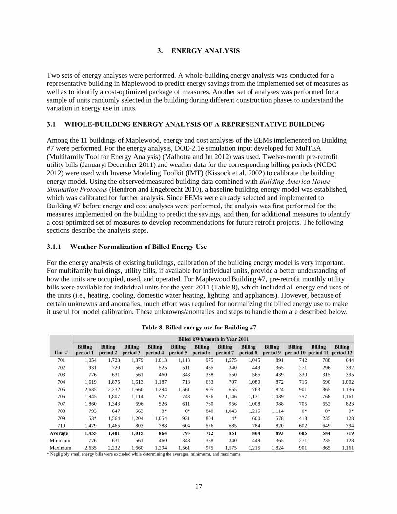
For the energy analysis of existing buildings, calibration of the building energy model is very important. For multifamily buildings, utility bills, if available for individual units, provide a better understanding of how the units are occupied, used, and operated. For Maplewood Building #7, pre-retrofit monthly utility bills were available for individual units for the year 2011 (Table 8), which included all energy end uses of the units (i.e., heating, cooling, domestic water heating, lighting, and appliances). However, because of certain unknowns and anomalies, much effort was required for normalizing the billed energy use to make it useful for model calibration. These unknowns/anomalies and steps to handle them are described below.

Table 8. Billed energy use for Building #7

Unit #

Billed kWh/month in Year 2011 Billing

period 1 Billing

period 2 Billing

period 3 Billing

period 4 Billing

period 5 Billing

period 6 Billing

period 7 Billing

period 8 Billing

period 9 Billing

period 10 Billing

period 11 Billing

period 12 701 1,054 1,723 1,379 1,013 1,113 975 1,575 1,045 891 742 788 644702 931 720 561 525 511 465 340 449 365 271 296 392703 776 631 561 460 348 338 550 565 439 330 315 395704 1,619 1,875 1,613 1,187 718 633 707 1,080 872 716 690 1,002705 2,635 2,232 1,660 1,294 1,561 905 655 763 1,824 901 865 1,136706 1,945 1,807 1,114 927 743 926 1,146 1,131 1,039 757 768 1,161707 1,860 1,343 696 526 611 760 956 1,008 988 705 652 823708 793 647 563 8* 0* 840 1,043 1,215 1,114 0* 0* 0*709 53* 1,564 1,204 1,054 931 804 4* 600 578 418 235 128710 1,479 1,465 803 788 604 576 685 784 820 602 649 794

Average 1,455 1,401 1,015 864 793 722 851 864 893 605 584 719Minimum 776 631 561 460 348 338 340 449 365 271 235 128Maximum 2,635 2,232 1,660 1,294 1,561 975 1,575 1,215 1,824 901 865 1,161

* Negligibly small energy bills were excluded while determining the averages, minimums, and maximums.

18

3.1.1.1 Handling unknowns and anomalies in utility bills

1. Anomalies in billed energy use across units

Table 8 shows that the billed energy use was negligibly small for some units during several billing periods. Assuming that these bills represent unoccupied periods, they were excluded from further analysis to determine if the remaining bills well represent the energy use during occupied periods. Fig. 27 shows the billed energy use during presumably occupied periods highlighting its variation across units, which is as much as 45% below average (for billing period 3) to 104% above average (for billing period 9). Furthermore, the ratio of highest to lowest bill for a specific billing period ranged from 2.7 (for billing period 8) to 9.1 (for billing period 12). Expecting the location and orientation of units in the building as possible factors for such variation, the utility bills were reviewed again by units. However, no correlation was found between location or orientation and utility bills. These variations suggest high irregularities in the occupancy, usage and operational characteristics of the units. To minimize the impact of these anomalies, further analysis was performed for the whole building, excluding the presumably unoccupied periods for which utility bills were negligibly small.

2. Anomalies in billed energy use across 12 months

Fig. 27 also shows that several units did not follow the typical weather-driven heating and cooling energy use profiles, and the energy use profiles were not consistent across units. Specifically, the billed energy use for billing periods 10, 11, and 12 was very small for most individual units for unexplainable reasons. Therefore, these billing periods were excluded from further analysis.

3. Unknown start and end dates of billing periods

The start and end dates of billing periods are required for weather normalization of billed energy use for energy model calibration. However, for this project, billing cycle dates could not be obtained. To ensure that the billed energy use align with the average temperature for the corresponding period, four scenarios for billing period start and end dates were assumed:

• Scenario 1: Billing cycle starting at the first day and ending at the last day of a month • Scenario 2: Billing cycle starting at day 8 of a month and ending at day 7 of the next month • Scenario 3: Billing cycle starting at day 15 of a month and ending at day 14 of the next month • Scenario 4: Billing cycle starting at day 22 of a month and ending at day 21 of the next month

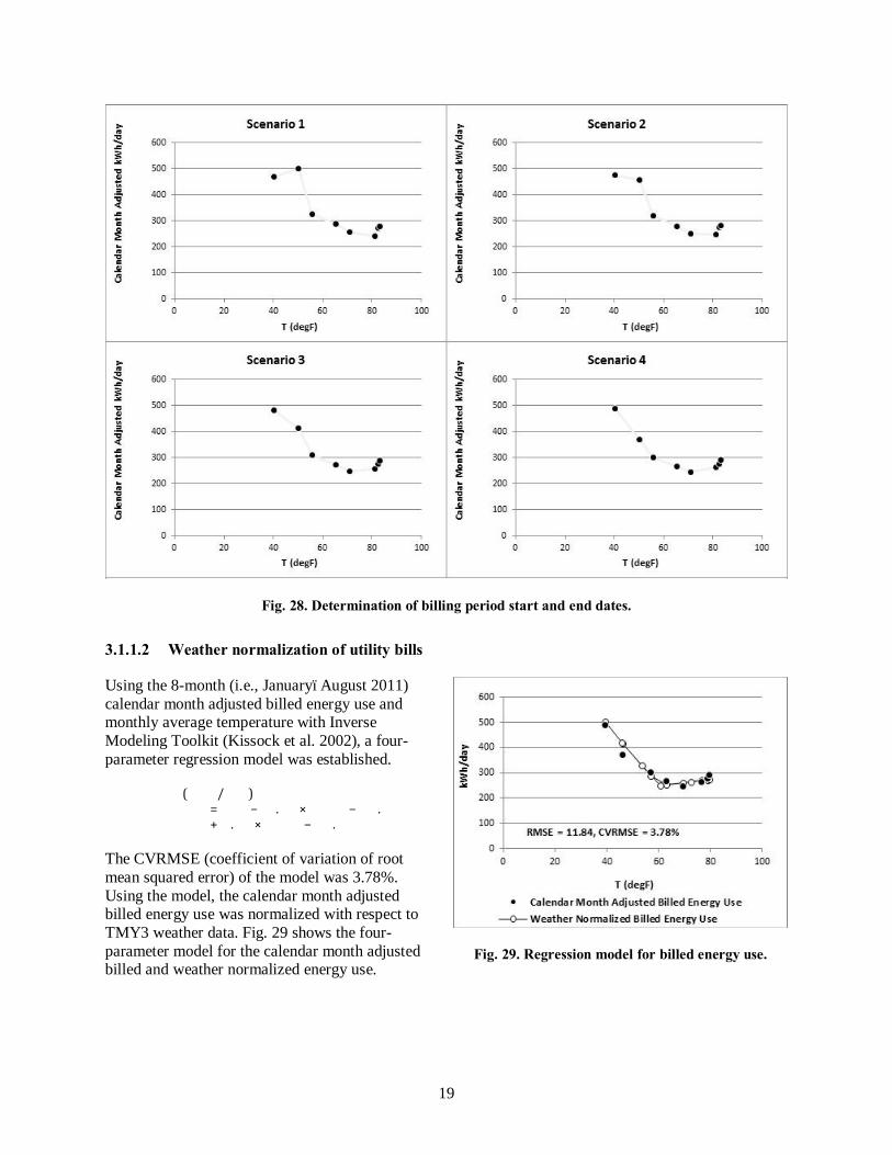
For each scenario, billed energy use was adjusted for the calendar months and plotted against monthly average temperatures for the year 2011. Fig. 28 shows the temperature-energy use scatter plot for the four scenarios described above. Among these, scenario 4 seems to have the best agreement between the energy use and temperature. Therefore, the billing period cycle for scenario 4 was selected for use in the next analysis steps.

Fig. 27. Cluster column plot of billed energy use.

19

Fig. 28. Determination of billing period start and end dates.

3.1.1.2 Weather normalization of utility bills

Using the 8-month (i.e., January–August 2011) calendar month adjusted billed energy use and monthly average temperature with Inverse Modeling Toolkit (Kissock et al. 2002), a four-parameter regression model was established.

���������(�� �/���)= ���− ��. �� × ���� � − ��. ���

+ �. �� × ���� � − ��. ���

The CVRMSE (coefficient of variation of root mean squared error) of the model was 3.78%. Using the model, the calendar month adjusted billed energy use was normalized with respect to TMY3 weather data. Fig. 29 shows the four-parameter model for the calendar month adjusted billed and weather normalized energy use.

Fig. 29. Regression model for billed energy use.

20

3.1.2 Calibration of Building Energy Model

As recommended in Hendron and Engebrecht (2010), utility bills were not heavily relied on as a tool for model validation, but used as an approximate check of model accuracy. This choice recognizes that (1) it is extremely difficult to accurately determine occupant behavior during the time period reflected in the utility bills and (2) the large number of uncertain input parameters allows multiple ways to reconcile the model with the small number of utility bills, and there is no reliable methodology for performing this calibration because the problem is mathematically undetermined. Having said this, a building energy model was developed using the known (observed/measured) building details and default values for unknown building details and the effects of maintenance and repairs (Hendron and Engebrecht 2010). TMY3 weather data were used in the energy simulation. Weather normalized billed energy use and simulated energy use were used in the model calibration.

Adjustments to building energy model inputs were made, including lighting and equipment energy use, heating and cooling months, and setpoint temperatures during heating and cooling months. After the final set of adjustments to the energy model, a good match could be established between the simulated and billed energy use. Fig. 30 shows the results of the calibrated simulation model – the weather-normalized and simulated monthly average daily energy use for the building. The CVRMSE was 10.99%. The calibrated model was used as the baseline against which the EEMs were evaluated. Table 15 summarizes the building characteristics of the calibrated building model. Appendix F describes how base-case characteristics were quantified.

Table 9. Baseline characteristics

Characteristic Description Comments

General

Building type and configuration

A 3-story, 10-unit multifamily building configured as two detached blocks, each consisting of a 2-bedroom unit and a vented crawlspace on level 1 (terrace level), and a 2-bedroom and a 3-bedroom unit on levels 2 and 3. The six 1048 ft2, 2-bedroom units and four 1260 ft2, 3-bedroom units amount to 11,328 ft2 of total building area

Modeled as two blocks of five 1132.8 ft2, 2.4-bedroom units arranged in the observed configuration

Surroundings Green grass (observed on three sides); No building-shading objects within 30 ft of the building

Modeled as 0.15 ground reflectance

Construction details

Above-grade walls

2×4 wood studs @ 16 in. o.c., R-13 high-density fiberglass batt cavity insulation

Modeled as R-11 to account for 19% R-value deratinga

Windows and glass doors

Single-pane, clear, aluminum frame windows; interior blinds; no exterior shading

Modeled as 1.31 U-value, 0.8 SHGC windowsb and 0.7 interior shading multipliera

Opaque doors Solid wood core Modeled as 0.49 U-value doors

Fig. 30. Calibrated simulation model compared with billed energy use data.

21

Characteristic Description Comments

Attic Unconditioned vented attic; 2×6 wood joists/rafters @ 24 in. o.c.; R-30 high-density glass fiber-batt attic insulation, dark asphalt shingle roofing

Modeled as R-24 to account for 19% R-value deratinga

Crawlspace Vented crawlspace; concrete masonry walls; deteriorated insulation between 2×10 wood joists/open truss system @ 24 in. o.c. of above-crawlspace floor

Model as 8 in. hollow concrete block walls, uninsulated above-crawlspace floor and sillbox

Slab-on-grade floor

Concrete slab, no perimeter insulation Modeled as 4 in. heavyweight concrete with no insulation; 80% carpet and 20% linoleum tile floor finish

Infiltration Ranging between 1,000 and 1,500 CFM50 for individual units, amounting to a whole-building infiltration of 12,058 CFM50; vented attic and vented crawlspace

Modeled as 0.424 ACH in units, 15 ACH in the attic, and 3 ACH in the crawlspace

Space conditions

Occupancy Unknown Modeled as 28 occupants, assuming 2 occupants in 2-bedroom units and 4 occupants in 3-bedroom units; consistent with BA Protocolsa

Lighting 18 incandescent lamps in 2-bedroom units; 20 incandescent lamps in 3-bedroom units; 2 T12 fluorescent lamps and a 15 W pin-base tube in all units

Modeled as 0.364 W/ft2 peak usage, adding 100% as sensible heat gain (See Appendix F)

Equipment Standard-efficiency appliances including a refrigerator, a dishwasher, and a cooking range/oven; Presence of a clothes washer, dryer, and miscellaneous appliances is unknown

Modeled as 0.512 W/ft2 equipment power density, adding 57% as sensible and 14% as latent heat gains (see Appendix F)

Schedulesa Unknown Modeled hourly schedules for occupancy, lighting and equipment (see Appendix F)

Mechanical systems

HVAC system 12 SEER, 7.5 HSPF central heat pump, air handler located in the conditioned space; heating and cooling capacity: 18 kBtu/h in the 2-bedroom units, 24 kBtu/h in the 3-bedroom units

Modeled as 10.63 SEER, 6.64 HSPF assuming 6-year age of the equipment and 3% maintenance factor (seldom or never maintained) a

HVAC system operation

Unknown Heating season: January through May and October through December; cooling season: April through Octobera

Setpoint temperature

Unknown Heating mode: 74°F with no setback period; cooling mode: 78°F with no setup period

DHW system A 40-gallon storage tank type electric water heater located in the conditioned space; deteriorated tank insulation on some water heaters; rated performance of 0.9 EF

Modeled as 0.87 EF assuming 19-year age of the equipment and 0.2% maintenance factor (seldom or never maintained)a; 0.98 recovery efficiency, 5.5 kW rated input

Domestic hot water use

Unknown Supply temperature: 130°F; hot water use calculated by month considering water mains temperature (see Appendix F).

Ducts Inside the conditioned space No duct loss modeled

a Source: Building America House Simulation Protocols (Hendron and Engebrecht 2010)

b Source: RESNET’s Mortgage Industry National Home Energy Rating Systems Standards (RESNET 2012)

22

3.1.3 Analysis of Energy Efficiency Measures

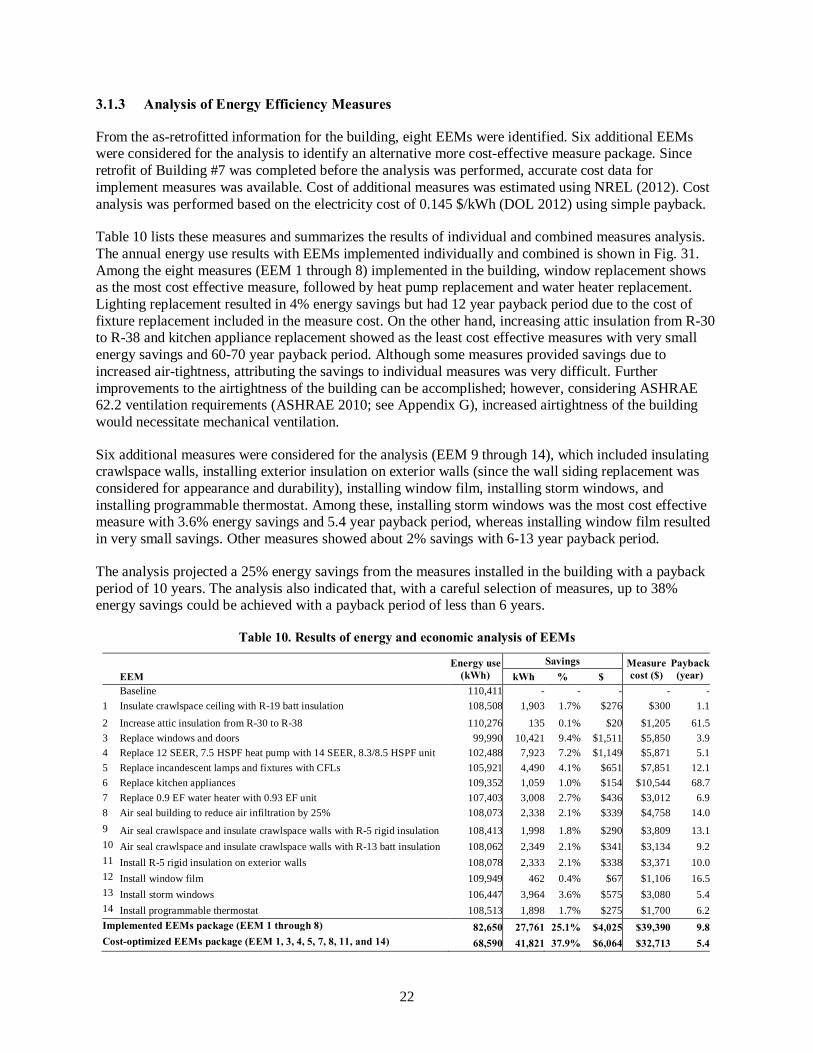
From the as-retrofitted information for the building, eight EEMs were identified. Six additional EEMs were considered for the analysis to identify an alternative more cost-effective measure package. Since retrofit of Building #7 was completed before the analysis was performed, accurate cost data for implement measures was available. Cost of additional measures was estimated using NREL (2012). Cost analysis was performed based on the electricity cost of 0.145 $/kWh (DOL 2012) using simple payback.

Table 10 lists these measures and summarizes the results of individual and combined measures analysis. The annual energy use results with EEMs implemented individually and combined is shown in Fig. 31. Among the eight measures (EEM 1 through 8) implemented in the building, window replacement shows as the most cost effective measure, followed by heat pump replacement and water heater replacement. Lighting replacement resulted in 4% energy savings but had 12 year payback period due to the cost of fixture replacement included in the measure cost. On the other hand, increasing attic insulation from R-30 to R-38 and kitchen appliance replacement showed as the least cost effective measures with very small energy savings and 60-70 year payback period. Although some measures provided savings due to increased air-tightness, attributing the savings to individual measures was very difficult. Further improvements to the airtightness of the building can be accomplished; however, considering ASHRAE 62.2 ventilation requirements (ASHRAE 2010; see Appendix G), increased airtightness of the building would necessitate mechanical ventilation.

Six additional measures were considered for the analysis (EEM 9 through 14), which included insulating crawlspace walls, installing exterior insulation on exterior walls (since the wall siding replacement was considered for appearance and durability), installing window film, installing storm windows, and installing programmable thermostat. Among these, installing storm windows was the most cost effective measure with 3.6% energy savings and 5.4 year payback period, whereas installing window film resulted in very small savings. Other measures showed about 2% savings with 6-13 year payback period.

The analysis projected a 25% energy savings from the measures installed in the building with a payback period of 10 years. The analysis also indicated that, with a careful selection of measures, up to 38% energy savings could be achieved with a payback period of less than 6 years.

Table 10. Results of energy and economic analysis of EEMs

Energy use (kWh)

Savings Measure cost ($)

Payback (year) EEM kWh % $

Baseline 110,411 - - - - -1 Insulate crawlspace ceiling with R-19 batt insulation 108,508 1,903 1.7% $276 $300 1.12 Increase attic insulation from R-30 to R-38 110,276 135 0.1% $20 $1,205 61.53 Replace windows and doors 99,990 10,421 9.4% $1,511 $5,850 3.94 Replace 12 SEER, 7.5 HSPF heat pump with 14 SEER, 8.3/8.5 HSPF unit 102,488 7,923 7.2% $1,149 $5,871 5.15 Replace incandescent lamps and fixtures with CFLs 105,921 4,490 4.1% $651 $7,851 12.16 Replace kitchen appliances 109,352 1,059 1.0% $154 $10,544 68.77 Replace 0.9 EF water heater with 0.93 EF unit 107,403 3,008 2.7% $436 $3,012 6.98 Air seal building to reduce air infiltration by 25% 108,073 2,338 2.1% $339 $4,758 14.09 Air seal crawlspace and insulate crawlspace walls with R-5 rigid insulation 108,413 1,998 1.8% $290 $3,809 13.110 Air seal crawlspace and insulate crawlspace walls with R-13 batt insulation 108,062 2,349 2.1% $341 $3,134 9.211 Install R-5 rigid insulation on exterior walls 108,078 2,333 2.1% $338 $3,371 10.012 Install window film 109,949 462 0.4% $67 $1,106 16.513 Install storm windows 106,447 3,964 3.6% $575 $3,080 5.414 Install programmable thermostat 108,513 1,898 1.7% $275 $1,700 6.2Implemented EEMs package (EEM 1 through 8) 82,650 27,761 25.1% $4,025 $39,390 9.8Cost-optimized EEMs package (EEM 1, 3, 4, 5, 7, 8, 11, and 14) 68,590 41,821 37.9% $6,064 $32,713 5.4

23

Fig. 31. Annual energy use for all EEMs.

3.2 ENERGY ANALYSIS OF SAMPLE UNITS

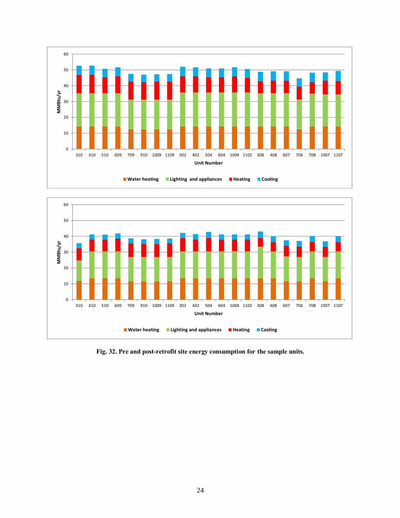
Using the diagnostic testing results and unit characteristics, REM/RateTM energy models were created to determine the estimated consumption in the sample units. Appendix D shows a comparison of the same unit type for pre- and post-energy-retrofit consumption based on the four major loads within the units: heating, cooling, water heating, and lighting and appliances. Using the software, a Home Energy Rating System (HERS) index was generated for both pre- and post-upgrade analysis. The average initial HERS index for the sample units was 107. The average final HERS index was 87, a 20% improvement from the average initial index. The mean initial annual site energy consumption for the units was 50 MMBtu and the mean post-retrofit consumption is 40 MMBtu, for an average estimated 18% in savings (Fig. 32).

0

30,000

60,000

90,000

120,000

150,000kW

h/ye

ar

DHW Lighting Equipment Heating Cooling Misc Vent fans

24

Fig. 32. Pre and post-retrofit site energy consumption for the sample units.

0

10

20

30

40

50

60

310 410 510 609 709 910 1009 1109 302 402 504 604 1004 1102 308 408 607 706 708 1007 1107

MM

Btu/

yr

Unit Number

Water heating Lighting and appliances Heating Cooling

0

10

20

30

40

50

60

310 410 510 609 709 910 1009 1109 302 402 504 604 1004 1102 308 408 607 706 708 1007 1107

MM

Btu/

yr

Unit Number

Water heating Lighting and appliances Heating Cooling

25

4. SUMMARY AND CONCLUSION Maplewood completed major renovations under the guidance of a third-party green building certification program in October 2012. Existing conditions were analyzed for one of the eleven Maplewood buildings, as well as for sample units selected across different buildings in the complex through visual assessment for general conditions and blower door measurements for envelope and duct leakage. For renovations, a whole-house approach was exercised: upgrading the building envelope with air-sealing, adding insulation, and replacing windows and replacing lighting, major appliances, heating and cooling systems, and domestic water heaters.

Because of the unique demands of this financing, including requirements for long-term ownership, the project aimed to add value to the property by improving the comfort, durability, and appearance of the building, as well as to provide energy and cost savings for the tenants. The project provided unique opportunities to learn about several aspects of a multifamily building retrofit that would benefit future projects in terms of improved building audit process, streamlined tasks, and higher energy savings. However, the project presented many challenges in accomplishing a number of tasks. Several missed opportunities were identified, some of which resulted from the challenges and some of which were not originally planned. The following sections describe these lessons learned.

In a previous study on a multifamily renovation with a similar scope of work, Flipper Temple (Kim et al. 2012), only 3% of the total construction cost was attributed to EEMs. Based on these two studies, less than 10% of a project’s construction cost is dedicated strictly to EEMs.

4.1 OPPORTUNITIES

Energy-saving opportunities

• Energy analysis of the sample units using REM/RateTM showed an average 20% reduction in the HERS index (pre-retrofit HERS index of 108 reduced to an index of 86 after the retrofit measures were implemented). Whole-building energy analysis of a typical 10-unit building of Maplewood showed a 25% savings projection from implemented measures.

Added property value

• All measures implemented in Maplewood greatly improved the appearance and durability of the buildings and its systems and improved thermal comfort for the occupants.

Learning opportunities

• By conducting unguarded and guarded blower door tests, it was possible to investigate the infiltration across the shared units.

• Comparing results of the two sets of energy analyses—one for sample individual units and one for the whole building—showed that the sampling set determined by the field team would be reasonably sufficient for whole-building energy analysis. At the same time, the results of a typical whole-building analysis could be generalized to similar buildings.

• The results of the detailed whole-building energy simulation to evaluate additional energy-retrofit measures emphasized the importance of having energy consultants involved at an early decision making stage.

26

4.2 CHALLENGES

During planning and decision making process

• Unlike in single-family audits, multiple team players are involved in multifamily housing audits— building owner, developer, contractor, architect, consultants, and tenants. Coordinating all involved parties requires extensive planning and execution, resulting in less flexibility.

• The application process for DCA QAP candidates did not involve the energy consultants in determining the EEMs. By the time developers approached Southface to implement a green building certification program, most of the EEMs had already been determined. Therefore, additional consultation could not be provided because the project schedule had already been initiated. Energy modeling iterations were produced after construction began. An evaluation of the process is necessary so that resources are optimized and expectations for every party involved are met.

• Different multifamily programs adhere to different sampling standards. For example, Maplewood is part of a third-party green building certification program that requires 33% sampling; additionally, Maplewood participated in a local utility rebate program that requires 15% sampling of units on each floor of a building. Consistency is important to effectively communicate a project’s design intent and to prevent confusion across teams.

Obtaining and interpreting utility data

• Acquiring utility bills is not a requirement for local program implementation of multifamily projects. Lack of access to unit-by-unit data or total building consumption prevents consultation on energy conservation measures by evaluating utility bills for a baseline. Based on the local utility company’s policy, individual tenant waivers must be signed. These waivers grant access to the building portfolio of the complex. Although pre-retrofit utility data were obtained for Maplewood, detailed billing information such as billing cycle dates could not be obtained. Such limitations presented challenges in weather normalizing the utility data and providing more accurate energy consumption characterizations. With QAPs driving many projects in the multifamily market, more research focus should be placed on how utility bills impact low-income families. If provided with such data, organizations such as DCA and HUD might be better able to market the value proposition of incorporating EEMs to lure developers to actively seek more affordable housing projects.

• More insight is needed to fully grasp the impact of EEMs on multifamily buildings. Researchers need information to resolve several issues related to occupancy levels and occupant characteristics:

– Uncertainty about occupancy details in units is an obstacle to benchmarking savings.

– Gaining access to occupancy level in each unit presents privacy issues, which could potentially hinder a project’s construction progress.

– Normalization of utility bills was difficult with unexplainable energy use profile observed in the utility bill data.

Implementation of measures

Selection of certain measures was based on cost, ignoring the ease of implementation, durability, and effectiveness of the measure. An example is the installation of floor insulation. Because of the significant cost difference between the quoted prices for spray foam ($1.50ft2) and batt insulation ($0.30/ ft2), the developers initially decided to use batt insulation under the framed floors. The open-web truss wood framing system made clean, proper installation between the framing members difficult. The field team had to make multiple quality assurance visits to Maplewood for each phase because of the shortcomings

27

found in the installation of batt insulation under the subfloor. The installers expressed frustration with the difficulty in achieving a clean, proper installation because of the challenges presented by the framing structure and plumbing lines. The additional costs for time and labor incurred to the developer due to extra effort should not be ignored while developing scopes of work.

Determining cost-effectiveness of retrofit measures

• Several building envelope measures (including adding attic insulation, roofing and wall siding replacement, window replacement, and installing above-crawlspace floor insulation) resulted in energy savings due to reduced conduction losses as well as supplemental benefits from reduced infiltration. The cumulative effect of these measures, combined with air-sealing, was observed through post-retrofit blower door tests. However, it was difficult to apportion the air-sealing benefits to individual measures. Thus energy savings and cost-effectiveness from these measures were underestimated because the energy savings did not account for savings due to reduction in air infiltration.

4.3 MISSED OPPORTUNITIES

Energy savings

Several energy savings opportunities were missed partly as a result of the late involvement of energy consultants and partly due to the selection criteria for retrofit measures. Detailed whole-building energy analysis of one of the buildings showed that

• Several measures implemented in the building resulted in very small and/or not cost-effective energy savings. These measures were implemented mainly to add value to the building. This is a common practice in multifamily buildings. However, such measures can be strategically selected or combined with other potential energy retrofit measures to result in an overall cost-effective package. For example, exterior wall siding was replaced, but not as an energy-retrofit measure. However, such a measure can be combined with adding exterior continuous insulation to provide energy savings for a lower installation cost than would be incurred otherwise. Roofing replacement, if considered from the standpoint of improving the long-term durability of the building, can result in energy savings if products with improved thermal properties are selected.

• With a careful selection of measures, energy savings of up to 37% could be achieved with a payback period of 6 years, whereas the EEMs implemented are projected to provide a 25% energy savings with 20 years of simple payback.

Human comfort and indoor air quality

Although improving comfort was one of the goals for this project, some comfort aspects were not considered in this project.

• Lighting replacement did not consider visual comfort (i.e., lighting level requirements) in different spaces of the units. The decision mainly considered incandescent wattage versus equivalent lower-wattage compact fluorescent light bulbs for lamps.

• The building envelope retrofit measures were selected mainly to reduce infiltration to the outdoors. In multifamily buildings, attention should also be given to air-sealing shared surfaces for reduced infiltration as well as improved acoustics of the units.

• ASHRAE 62.2-2010 (ASHRAE 2010) calculations with pre-retrofit guarded blower door measurements and exhaust deficits in the bathrooms and kitchen revealed that the units were under-ventilated. The air-sealing retrofit measure decreased the air infiltration rate by about 25% and

28

required a higher mechanical ventilation rate to comply with ASHRAE 62.2. However, no consideration was given to achieving compliance with ASHRAE 62.2 and providing mechanical ventilation.

• For replacement of HVAC systems, post-retrofit system sizing calculations were not performed. The replacement HVAC systems were selected based on the sizes of the existing systems. Post-retrofit reduced loads may result in system oversizing and increased cycling of systems, thereby reducing performance and thermal comfort in the units.

29

REFERENCES ACE (US Army Corps of Engineeers). 2012. U.S. Army Corps of Engineers Air Leakage Test Protocol

for Building Envelopes, Version 3. Construction Engineering Research Laboratory, U.S. Army Engineer Research and Development Center, Champaign, IL, May 11.

ASHRAE (American Society of Heating, Refrigeration and Air-Conditioning Engineers, Inc.). 2010. ANSI/ASHRAE Standard 62.2-2010, Ventilation and Acceptable Indoor Air Quality in Low-Rise Residential Buildings. American Society of Heating, Refrigerating and Air-Conditioning Engineers, Inc., Atlanta, GA.

ASTM (American Society for Testing and Materials). 2010. ASTM E799-10, Standard Test Method for Determining Air Leakage Rate by Fan Pressurization. ASTM International, West Conshohocken, PA.

DOL (US Department of Labor). 2012. Average Energy Prices in Atlanta—July 2012, Southeast Information Office, Bureau of Labor Statistics. Retrieved July, 2012, from http://www.bls.gov/ro4/aepatl.htm.

Energy Conservatory. 2010. Example Multi-Fan Airtightness Test with TECLOG2, Setting up and Conducting a Test. The Energy Conservatory, Minneapolis, MN.

Energy Conservatory. 2012. Mineapolis Blower DoorTM Operation Manual for Model 3 and Model 4 Systems. The Energy Conservatory, Minneapolis, MN.

GDCA (Georgia Department of Community Affairs). 2010. 2010 Qualified Allocation Plan. Office of Affordable Housing, Georgia Department of Community Affairs, Atlanta, GA.

Hendron, R. and C. Engebrecht. 2010. Building America House Simulation Protocols, DOE/GO-102010-3141, National Renewable Energy Laboratory, Golden, CO.

HUD (U.S. Department of Housing and Urban Development). 2010. LIHTC Basics. Retrieved February 22, 2012, from: http://www.hud.gov/offices/cpd/affordablehousing/training/web/lihtc/basics/.

International Code Council. 2009. 2009 International Building Code. Washington, DC: International Code Council, Inc.

Kim, E., R. Stephenson, S. Reberts, J. Yoo, M. Monroe, and P. Im. 2012. Case Study of the Flipper Temple Multifamily Retrofit for Energy Efficiency. ORNL/TM-2012/167. Oak Ridge National Laboratory, Oak Ridge, TN.

Kissock, J. K., J. S. Haberl, and D. E. Claridge 2002. Development of a Toolkit for Calculating Linear, Change-point Linear and Multiple-Linear Inverse Building Energy Analysis Models, ASHRAE Research Project 1050-RP, American Society of Heating, Refrigeration and Air-conditioning Engineers, Inc., Atlanta, GA.

Lutz, J., C. D. Whitehead, A. Lekov, D. Winiarski, and G. Rosenquist 1998. “WHAM: A Simplified Energy Consumption Equation for Water Heaters,” in Proceedings of the 1998 ACEEE Summer Study on Energy Efficiency in Buildings 1:171–183, American Council for an Energy-Efficient Economy, Pacific Grove, CA.

30

Malhotra, M. and P. Im. 2012. “Development of a Flexible Multizone Multifamily Building Simulation Model,” in Proceedings of SimBuild 2012–5th National Conference of IBPSA–USA, Madison, Wisconsin, August 1–3, International Building Performance Simulation Association.

NCDC (National Climatic Data Center). 2012. Quality Controlled Local Climatological Data. National Oceanic and Atmospheric Administration. Available at http://www.ncdc.noaa.gov/land-based-station-data/quality-controlled-local-climatological-data-qclcd.

NREL (National Renewable Energy Laboratory). 2012. National Energy Efficiency Measures Database. Available at http://www.nrel.gov/ap/retrofits/group_listing.cfm.

RESNET (Residential Energy Services Network). 2011. RESNET Standard for Performance Testing and Work Scope: Enclosure and Air Distribution Leakage Testing, Chapter 8: 803.2, “RESNET Simplified Test Procedures,” Residential Energy Services Network, Oceanside, CA.

RESNET (Residential Energy Services Network). 2012. 2006 Mortgage Industry National Home Energy Rating Systems Standards with 2012 Enhancements. Residential Energy Services Network, Oceanside, CA.

APPENDIX A MAPLEWOOD ARCHITECTURAL PLANS

A-3

APPENDIX A. MAPLEWOOD ARCHITECTURAL PLANS

Unit A (two-bedroom unit).

Unit B (three-bedroom unit).

A-4

Unit C (three-bedroom unit).

APPENDIX B MAPLEWOOD PHOTOGRAPHS

B-3

APPENDIX B. MAPLEWOOD PHOTOGRAPHS

Pre-Retrofit Photographs

Interior spaces

Wall penetrations

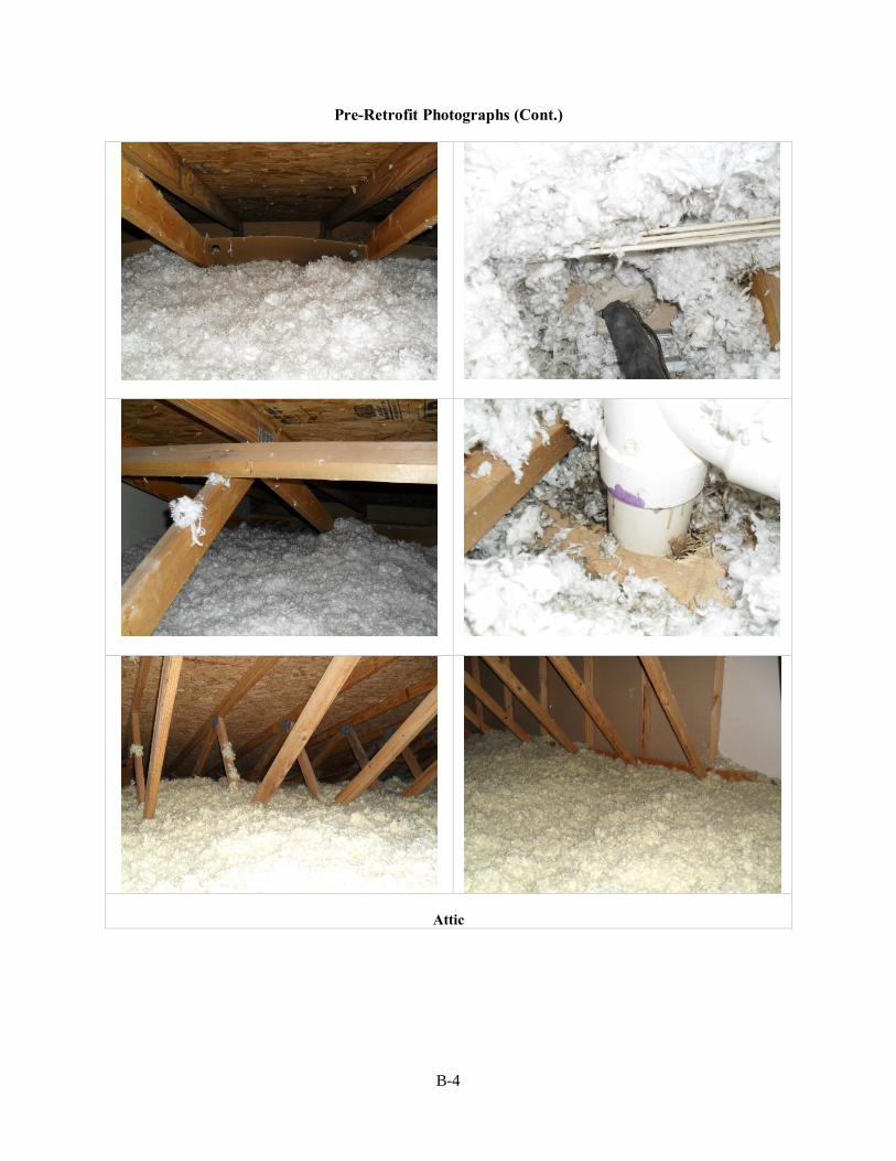
B-4

Pre-Retrofit Photographs (Cont.)

Attic

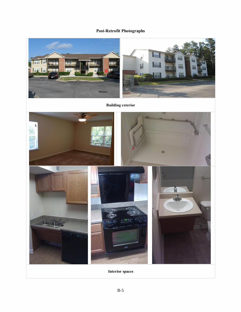
B-5

Post-Retrofit Photographs

Building exterior

Interior spaces

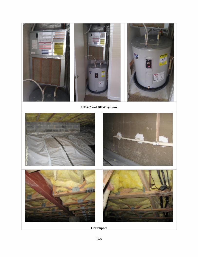
B-6

HVAC and DHW systems

Crawlspace

B-7

Attic

APPENDIX C MAPLEWOOD QAP SUSTAINABILITY CHECKLIST

C-3

APPENDIX C. MAPLEWOOD QAP SUSTAINABILITY CHECKLIST

C-4

C-5

APPENDIX D DIAGNOSTIC TEST DATA FOR SAMPLE UNITS

D-3

APPENDIX D. DIAGNOSTIC TEST DATA FOR SAMPLE UNITS

Unit # Type Conditioned

floor area (ft2)

Envelope leakage Duct leakage

Pre-retrofit Post-retrofit Leakage reduction

(%)

Pre-retrofit Post-retrofit Leakage reduction

(%)

Blower door fan

flow (CFM50)

ACH50

Blower door fan

flow (CFM50)

ACH50

Duct blaster

fan flow (CFM25)

Leakage to outside (%)

Duct blaster

fan flow (CFM25)

Leakage to outdoors (%)

Terrace floor 310 B 1,176 1,739 11.1 1,190 7.6 31.6% 10 0.9% 4 0.3% 0.5% 410 B 1,176 1,664 10.6 907 5.8 45.5% 30 2.6% 20 1.7% 0.9% 510 B 1,176 1,720 11.0 848 5.4 50.7% 12 1.0% 12 1.0% 0.0% 609 B 1,176 1,807 11.5 1,201 7.7 33.5% 22 1.9% 22 1.9% 0.0% 709 A 1,049 1,520 10.9 1,227 8.8 19.3% 8 0.8% 26 2.5% -1.7% 910 A 1,049 1,530 10.9 942 6.7 38.4% 18 1.7% 12 1.1% 0.6%

1009 A 1,049 1,983 14.2 1,064 7.6 46.3% 18 1.7% 34 3.2% -1.5% 1109 A 1,049 1,050 7.5 1,050 7.5 0.0% 25 2.4% 25 2.4% 0.0%

Second floor 302 B 1,176 1,336 8.5 990 6.3 25.9% 114 9.7% 20 1.7% 8.0% 402 B 1,176 1,462 9.3 954 6.1 34.7% 24 2.0% 30 2.6% -0.5% 504 C 1,260 1,301 7.7 1,033 6.1 20.6% 17 1.3% 16 1.3% 0.1% 604 B 1,176 967 6.2 967 6.2 0.0% 39 3.3% 39 3.3% 0.0%

1004 C 1,260 1,691 10.1 966 5.8 42.9% 22 1.7% 18 1.4% 0.3% 1102 B 1,176 958 6.1 958 6.1 0.0% 27 2.3% 27 2.3% 0.0%

Third floor 308 B 1,176 1,324 8.4 1,021 6.5 22.9% 711 60.5% 28 2.4% 58.1% 408 B 1,176 1,427 9.1 901 5.7 36.9% 22 1.9% 108 9.2% -7.3% 607 B 1,176 1,252 8.0 1,252 8.0 0.0% 19 1.6% 19 1.6% 0.0% 706 A 1,049 1,252 9.0 1,135 8.1 9.3% 14 1.3% 20 1.9% -0.6% 708 C 1,260 1,201 7.1 1,023 6.1 14.8% 40 3.2% 26 2.1% 1.1%

1007 A 1,049 1,427 10.2 967 6.9 32.2% 20 1.9% 8 0.8% 1.1% 1107 A 1,049 911 6.5 911 6.5 0.0% 25 2.4% 25 2.4% 0.0%

Average 9.2 6.7 24.1% 5.1% 2.2% 2.8%

APPENDIX E CALIBRATION RESULTS

E-3

APPENDIX E. CALIBRATION RESULTS

Weather normalization of billed energy use

Jan Feb Mar Apr May Jun Jul Aug Sep Oct Nov DecYear 2011 temperature (°F) 40.2 50.0 55.8 65.3 70.9 81.3 82.4 83.1 73.3 62.2 55.7 50.5Year 2011 billed energy use (kWh/day)

490 371 301 266 246 264 277 292 226 195 221 232

Year 2011 predicted energy use (kWh/day)

491 370 299 255 262 275 276 277

Residual, billed—predicted −0.5 0.3 1.6 10.5 −16.4 −10.7 0.9 14.3Residual, billed—predicted (%) −0.1 0.1 0.5 4.1 −6.3 −3.9 0.3 5.2

���������(�� �/���) = ���− ��. �� × ���� � − ��. ��� + �. �� × ���� � − ��. ��� RMSE = 11.84, CVRMSE = 3.78% TMY3 temperature (°F) 39.2 46.2 56.8 63.0 69.4 76.6 79.0 79.7 72.5 60.8 53.4 45.9Weather-normalized billed energy use (kWh/day)

503 417 286 252 260 269 272 273 264 249 328 421

Comparison of weather normalized utility bills and calibrated building energy model

Jan Feb Mar Apr May Jun Jul Aug Sep Oct Nov DecTMY3 temperature (°F) 39.2 46.2 56.8 63.0 69.4 76.6 79.0 79.7 72.5 60.8 53.4 45.9Weather-normalized billed energy use (kWh/day) 503 417 286 252 260 269 272 273 264 249 328 421

Simulated energy use (kWh/day) 433 387 274 243 245 290 303 309 252 237 291 370Residual, weather-normalized—simulated 70 30 12 9 15 -21 -30 -36 12 12 37 52Residual, weather-normalized—simulated (%) 13.9% 7.1% 4.3% 3.6% 5.9% -7.8% -11.2% -13.3% 4.7% 4.9% 11.3% 12.2%

RMSE = 35, CVRMSE = 11.99%

APPENDIX F CONSIDERATIONS FOR WHOLE-BUILDING ENERGY ANALYSIS

E-3

APPENDIX F. CONSIDERATIONS FOR WHOLE-BUILDING ENERGY ANALYSIS F.1 Estimation of Lighting Power Density

The pre-retrofit hardwired lighting system consisted of eighteen 60W incandescent lamps, two T-12 fluorescent lamps, and a 15 W lamp over the sink in two-bedroom units and twenty-one 60 W incandescent lamps, two T-12 fluorescent lamps, and a 15 W lamp over the sink in three-bedroom units. For the post-retrofit hardwired lighting system, all incandescent lamps were replaced with 13W compact fluorescent lamps and more efficient (lower wattage) fluorescent lamps. The wattage and distribution of pre- and post-retrofit hardwired lighting system characteristics are shown in Table F.1. With these characteristics, the average hardwired lighting power density was 1.10 W/ft2 before the retrofits and 0.29 W/ft2 after the retrofits. No change in the plug-in lighting system was assumed. Pre- and post-retrofit lighting energy use was modeled using the peak lighting W/ft2 use (derived from the benchmark lighting budget combined with the adjustments for installed hardwired lighting system characteristics, as shown in Table F.2) and the usage schedule (Fig. F.1).

Table F.1. Pre- and post-retrofit hardwired lighting system characteristics

Space

Number of lamps Lamp wattage Installed wattage

2-bedroom unit

3-bedroom unit

Pre-retrofit

Post-retrofit

Pre-retrofit Post-retrofit 2-bedroom

unit 3-bedroom

unit 2-bedroom

unit 3-bedroom

unit Bedrooms 4 6 60 13 240 360 52 78 Bathrooms 8 8 60 13 480 480 104 104 Closet/store 2 3 60 13 120 180 26 39 Hallway 2 2 60 13 120 120 26 26 Living room 2 2 60 13 120 120 26 26 Kitchen (T-12) 2 2 40 32 80 80 64 64 Kitchen (15 W over the sink) 1 1 15 15 15 15 15 15 Installed wattage 1175 1355 313 352 W/ft2 1.121 1.075 0.299 0.279 Average W/ft2 1.10 0.29

Table F.2. Pre- and post-retrofit lighting energy use calculations Lamp type Lamp efficacy (Efflamp)

lm/W Default lamp type

fraction (Fdefault,lamp)

Installed lamp type fraction (Finstalled,lamp)

Pre-retrofit Post-retrofit Incandescent 15 66% 94% 0% CFL 55 21% 0% 80% LED 50 0% 0% 0% T8 88 13% 0% 0% T12 82 0% 6% 20% Lighting energy use (assuming default lamp types)

Interior hardwired lighting (kWh/year) LHW = 0.8*(FFA*0.542+334) 758.4 Interior plug-in lighting (kWh/year) LPlug = 0.2*(FFA*0.542+334) 189.6

Adjustments Pre-retrofit Post-retrofit

Lamp type adjustment factor AdjLampType = 1 +Σ[(Finstalled,lamp - Fdefault,lamp)*Efflamp/Effincand] 1.208 0.516 Smart lamp replacement factor SRF = 1.1*FInc

4 - 1.9*FInc3 + 1.5*FInc

2 - 0.7* FInc + 1 – 1.08 Take back 10% for lamp replacement (post-retrofit) – 10% Adjusted hardwired lighting (kWh/year) LHW,adj = LHW *[ AdjLampType * SAF * 0.9 + 0.1 ] 916 467 Total lighting energy use (kWh/year) LTotal = LHW,adj + LPlug 1105.6 656.6 Average daily lighting energy use (kWh/day) Ldaily = LTotal/365 3.03 1.80 Peak W/ft2 Lpeak WSF = Ldaily * Peak Fraction of Daily Sum 0.364 0.216

8 Smart lamp replacement factor was ignored, since all lamps were replaced (as opposed to the replacement of high-use lamps first).

E-4

Fig. F.1. Lighting schedule.

E-5

F.2 Estimation of Equipment Power Density

Equipment power density (EPD) was estimated for an average unit assuming all-electric appliances including a refrigerator, dishwasher, cooktop/oven, clothes washer, clothes dryer, and miscellaneous appliances commonly found in a multifamily unit. The energy use for these appliances was estimated using the Building America Simulation Protocols combined with the federal standard for appliance energy performance for the pre-retrofit case and rated energy performance for the post-retrofit case. Table F.3 shows the pre and post-retrofit appliance characteristics and EPD. These values combined with the equipment schedule (Fig. F.2) were used for modeling the equipment energy use.

Table F.3. Pre- and post-retrofit equipment characteristics and energy use

Equipment Description Energy use (kWh/year)

Pre-retrofit Post-retrofit Refrigerator Pre-retrofit: Building America Simulation Protocols (434 kWh/year)

Post-retrofit: Whirlpool WRT138TFYB (388 kWh/year) 434 388

Dishwasher Pre-retrofit: 0.6 EF Post-retrofit: Whirlpool DU850SWP (306 kWh/year => 0.7 EF)

Annual energy use = Machine energy use fraction * Number of cycles per year / EFdishwasher

Machine energy use fraction = 44% Number of cycles per year = 215*(1/2 + Nbr/6)

142 121

Cooktop/oven Pre-retrofit: Assumed characteristics: Cooktop: Non-reflective pans, rounded coil elements (73.7% EF) Oven: Standard door seals, standard vent rate, standard insulation (10.9% EF)

Post-retrofit: Whirlpool RF114PXSB; Assumed characteristics: Cooktop: Reflective pans, flat coil elements (77.7% EF) Oven: Improved door seals, reduced vent rate, high-density insulation (12.1% EF)

Annual energy use = (86.5 + 28.9*Nbr)/EFcooktop + (14.6 + 4.9*Nbr)/EFoven

453 418

Clothes washer Pre-retrofit: Building America Simulation Protocols Post-retrofit: No change Annual energy use = (38.8 + 12.9*Nbr)

70 70

Clothes dryer Pre-retrofit: Building America Simulation Protocols Post-retrofit: No change Annual energy use = (538.2 + 179.4*Nbr)

969 969

Miscellaneous electrical loads (MELs)

Pre-retrofit: Building America Simulation Protocols assuming the following appliances: A microwave, a toaster, a blender, a TV, a DVD player, ceiling fans in each bedroom, an iron, a smoke detector, a doorbell, a desktop PC and monitor, a vacuum cleaner, a cordless phone charger, 2 cellphone chargers, an answering machine, and air handler standby losses.

Post-retrofit: No change

1,275 1,275

Total kWh/year 3343 3241 W/ft2 1000* [Annual Energy Use / Hours of Operation per Year] / Average Area of a Unit 0.512 0.496

Fig. F.2. Equipment schedule.

E-6

F.3 Estimation of Internal Heat Gains

Internal heat gains from appliances were estimated using the latent and sensible load fractions as shown in Table F.4, and modeled as sensible and latent heat gain fractions combined with the equipment usage schedule (Fig. F.2). The combined sensible and latent heat gain fractions were 0.565 and 0.143 for the pre-retrofit case and 0.545 and 0.138 for the post-retrofit case.

Table F.4. Pre- and post-retrofit internal heat gains from household appliances

Appliance

Sensible load

fraction

Latent load

fraction

Pre-retrofit Post-retrofit

Annual energy use (kWh/year)

Sensible heat gains

(kWh/year)

Latent heat gains

(kWh/year)

Annual energy use (kWh/year)

Sensible heat gains

(kWh/year)

Latent heat gains

(kWh/year) Refrigerator 1.0 0.0 434 434 – 388 388 – Dishwasher 0.60 0.15 142 85 21 121 73 18 Range 0.40 0.30 453 181 136 418 167 126 Clothes washer 0.80 0.0 70 56 – 70 56 – Clothes dryer 0.15 0.05 969 145 48 969 145 48 MELs 0.734 0.20 1275 936 255 1275 936 255 Total (kWh/year) 1889 478 1.765 447 Internal heat gain fraction 0.565 0.143 0.545 0.138

Internal heat gains from domestic hot water use in shower, bath, and sink were estimated as shown in Table F.5 and modeled as sensible and latent heat gain fractions of source Btu/h combined with the domestic hot water usage schedule (Fig. F.3) for both pre and post-retrofit cases. The combined internal heat gains were estimated as 3,745 Btu/h with sensible and latent heat gain fractions of 0.594 and 0.406, respectively.

Table F.5. Internal heat gains from domestic hot water use

Sensible heat gains

(Btu/day) Latent heat gains

(Btu/day) Comments Shower 1,334 1,267 Sensible: 741 + 247*Number of Bedrooms

Latent: 703 + 235* Number of Bedrooms Bath 334 – Sensible: 185 + 62* Number of Bedrooms

Latent: Negligible Sink 557 253 Sensible: 310 + 103* Number of Bedrooms

Latent: 140 + 47* Number of Bedrooms Total 2,225 1,520 Internal heat gain fraction 0.594 0.406 a Internal heat gains from dishwasher and clothes washer use are modeled as part of the internal gains from appliances (included in Table G.4).

Fig. F.3. Domestic hot water use schedule.

E-7

The building was modeled with 2.8 occupants per unit, 220 Btu/h per occupant of sensible heat gains, and 164 Btu/h per occupant of latent heat gains. Internal heat gains from occupants were modeled with the occupancy schedule shown in Fig. F.4.

Fig. F.4. Occupancy schedule.

E-8

F.4 Estimation of Domestic Hot Water Use

First, the base-case domestic hot water use by end-use was calculated for an average 2.4-bedroom unit, which adds up to 8.3 gal/day of hot water use at 130°F and 54.0 gal/day of hot water use at 110°F (as shown in Table F.6).

Table F.6. Domestic hot water consumption by end-use Number of bedrooms (Nbr) = 2.4 End use End-use water

temperature Water usage

(gal/day) Base-case water usage

(gal/day) Total (Vmixed,N)

(gal/day) Clothes washer 130°F 2.35 + 0.78 * Nbr (Hot Only) 4.2

Vhot,130ºF = 8.3 Dishwasher 130°F 2.26 + 0.75 * Nbr (Hot Only) 4.1 Shower 110°F 14.0 + 4.67 * Nbr (Hot + Cold) 25.2

Vmixed,110ºF = 54.0 Bath 110°F 3.5 + 1.17 * Nbr (Hot + Cold) 6.3 Sinks 110°F 12.5 + 4.16 * Nbr (Hot + Cold) 22.5

Next, the monthly average water mains temperature was calculated for an average day of each month using the Building America Simulation Protocols to account for the impact of location and time of year (Fig. G.5). Finally, the monthly average daily domestic hot water use at a 130°F supply temperature was calculated for each location to account for the use of cold water at mains temperature to achieve the required mixed temperature for various hot water end uses.

V (gal/day) = Vhot,130ºF + Vmixed,110ºF * (110 – Tmains) / (130 – Tmains)

The calculated hot water supply volume is plotted in Fig. F.5, which was used for the analysis of domestic hot water energy use and associated retrofit measures.

Fig. F.5. Water mains temperature and domestic hot water use.

E-9

F.5 Analysis of Domestic Hot Water Energy Use

The characteristics of the existing and replacement water heater are shown in Table F.7.

Table F.7. Water heater characteristics

Pre-retrofit Post-retrofit

Energy factor 0.9 (modeled as 0.87a) 0.93

Recovery efficiency 0.98 0.98

Burner capacity (Btu/h) 5.5 kW 5.5 kW

Tank UA (Btu/h⋅°F) 3.74 1.53

aThis accounts for 19 year age of equipment and 0.002 maintenance factor. Analysis of domestic hot water energy use was performed using the WHAM model (Lutz 1998) for the existing and the replacement electric water heater. Table F.8 shows the domestic hot water energy use with the existing and replacement water heater. The analysis used a 130°F supply water temperature, a 74°F ambient temperature, and monthly variation in water mains temperature as shown in Fig. F.5. With these inputs, the replacement electric water heater resulted in a 10% water heating energy savings.

Table F.8. Domestic hot water energy use

Month Tmains (°F) Vh (gpd) Pre-retrofit Post-retrofit

kBtu/ day kWh/mo. kBtu/ day kWh/mo. Jan 56.7 47.5 34.2 3,108 31.4 2,856 Feb 56.5 47.6 34.3 2,816 31.5 2,589 Mar 59.3 47.0 32.9 2,986 30.1 2,734 Apr 64.3 45.8 30.2 2,659 27.4 2,413 May 70.3 44.2 27.1 2,464 24.3 2,208 Jun 75.7 42.4 24.3 2,138 21.5 1,889 Jul 79.0 41.1 22.6 2,050 19.7 1,791 Aug 79.5 40.9 22.3 2,028 19.5 1,769 Sep 77.0 41.9 23.6 2,079 20.8 1,829 Oct 72.1 43.6 26.2 2,380 23.4 2,123 Nov 66.1 45.4 29.3 2,576 26.5 2,330 Dec 60.6 46.7 32.2 2,922 29.4 2,669 Total

30,207

27,199

Energy savings

10.0%

APPENDIX G ASHRAE STANDARD 62.2 COMPLIANCE CHECK

G-3

APPENDIX G. ASHRAE STANDARD 62.2 COMPLIANCE CHECK Calculations for ventilation requirements using ASHRAE Standard 62.2-2010 (ASHRAE 2010) were performed for an average unit of the building for pre- and post-retrofit cases using the pre- and post-retrofit multi blower door measurements (Table G.1). For the pre-retrofit case, a 25 CFM local exhaust deficit (due to recirculating-type kitchen exhaust fans), minus a 21 CFM infiltration credit (due to 1206 CMF@50 PA) resulted in a 41 CFM mechanical ventilation requirement. For the post-retrofit case, a 25 CFM local exhaust deficit due to the recirculating-type kitchen exhaust fan, minus the 13 CFM infiltration credit ([due to 898 CMF@50 PA] after air sealing the building) resulted in a 49 CFM mechanical ventilation requirement.

Table G.1. Minimum mechanical ventilation requirement in a unit

Inputs Pre-retrofit Post-retrofit Comments State-City GA-Atlanta GA-Atlanta

Apartment floor area 1132.8 ft2 1132.8 ft2 Average

Average floor height 8 ft 8 ft

Height of the building 24 ft 24 ft

Number of occupants 2.8 2.8 Assumed

Number of bedrooms 2.4 2.4 Average

Number of bathrooms 2 2

Bathroom 1: Exhaust fan 50 CFM 50 CFM Vented to outside; Assumed fan flow

Bathroom 2: Exhaust fan 50 CFM 50 CFM Vented to outside; Assumed fan flow

Kitchen Exhaust fan 0 0 Not vented to outside

Measured infiltration rate 1,206 CFM@50Pa 898 CFM@50 Average

Intermediate calculations

Leakage area (ASTM 779) 0.46 ft2 0.34 ft2 ��� @50 × 0.055/144

Normalized leakage 0.57 0.42 1000 �����������

���������× �

���������ℎ�8

��.�

Weather factor 0.75 0.75 From ASHRAE 136-1993 (RA 2006)

Air change rate from infiltration 0.42 ACH 0.32 ACH ���� ������������� × � ���ℎ��������

Infiltration flow rate 64 CFM 48 CFM ��������������� × ����� �/60

Default infiltration credit 23 CFM 23 CFM 0.02 × ���������

Excess infiltration 41 CFM 25 CFM ���������������� ����− �������������������

Results

Ventilation air requirement 37 CFM 37 CFM 0.01 × ��������� + 7.5× ���� ������������ �+ 1�

Deficit for higher occupant density 0 0 7.5 × ���� ��������������− ���� ������������ �+ 1���

Local exhaust deficit 25 CFM 25 CFM 0.25 × �� �50 − �������

����

+ �100 − �����������

Infiltration credit 21 CFM 13 CFM − 0.5 × ������������������

Mechanical ventilation requirement 41 CFM 49 CFM ����������������������������������� ��� + �������ℎ�����������− ������������������

APPENDIX H ENEGY EFFICINCY MEASURE DESCRIPTION AND COST DATA

H-3

APPENDIX H: ENERGY EFFICIENCY MEASURES DESCRIPTION AND COST DATA

Energy efficiency measures

Measure description

Measure cost for Building #7 Pre-retrofit characteristics Post-retrofit characteristics

1 Insulate crawlspace ceiling No insulation R-19 fiberglass batt insulation $300 (installed cost)

2 Add attic insulation R-30 blown-in fiberglass insulation

R-38 blown-in fiberglass insulation

$1,205 (installed cost)

3 Window and door replacement

Single pane, aluminum frame windows, solid wood core doors

Low-e, double pane, vinyl frame windows, insulated core metal doors

$5,850 (installed cost)

4 HVAC system replacement 12 SEER, 7.5 HSPF heat pump

14.5 SEER, 8.3/8.5 HSPF heat pump

$5,871 (installed cost)

5 Lighting replacement 60 W incandescent lamps 16 W compact fluorescent lamps $7,851 (installed cost)

6 Kitchen appliance replacement

Standard efficiency cooking range/oven, refrigerator and dishwasher

cooking range/oven with high-speed coil elements, Energy Star qualified refrigerator and dishwasher

$10,544 (installed cost)

7 Domestic water heater replacement

0.9 EF electric water heater 0.93 EF electric water heater $3,012 (installed cost)

8 Air seal building envelope Air leakage reduced by 25% $4,758 ($0.42 per ft2 of floor areaa)

9 Air seal crawlspace and install rigid insulation on crawlspace walls

Vented crawlspace with 3 ACH infiltration rate, no insulation

Unvented crawlspace with 0.5 ACH infiltration rate, R-5 XPS insulation on crawlspace walls

$3,809 ($1.3 per ft2 of crawlspace wall area for installing insulation, $0.72 per ft2 of crawlspace floor area for air sealinga)

10 Air seal crawlspace and install batt insulation on crawlspace walls

Vented crawlspace with 3 ACH infiltration rate, no insulation

Unvented crawlspace with 0.5 ACH infiltration rate, R-19 fiberglass batt insulation on crawlspace walls

$3,134 ($0.86 per ft2 of crawlspace wall area for installing insulation, $0.72 per ft2 of crawlspace floor area for air sealinga)

11 Install rigid insulation on exterior walls

No exterior insulation R-5 XPS insulation $3,371 ($0.98 per ft2 of wall area for adding insulation when replacing sidingb)

12 Install window film - Reduced effective window SHGC to 0.6

$1,106 ($2.25 per ft2 of window areab)

13 Install storm windows - Reduced effective window U-value and SHGC

$3,080 ($70 per windowb)

14 Install programmable thermostat

No night setback and afternoon setup

Night setback to 68°F and afternoon setup to 78°F for 6 hours

$1,700 ($170 per unita)

a Source: National Energy Efficiency Measures Database (NREL 2012). bSource: PNNL database

APPENDIX I REM/RATETM RESULTS FOR ENERGY ANALYSIS OF SAMPLE UNITS

I-3

APPENDIX I. REM/RATETM RESULTS FOR ENERGY ANALYSIS OF SAMPLE UNITS

Unit # Type

Pre-retrofit Post-retrofit Difference (%)

Energy Use (MBtu/h)

HERS Index

Energy Use (MBtu/h)

HERS index

Energy use

Hea

ting

Coo

ling

Wat

er h

eatin

g

Lig

htin

g an

d ap

plia

nces

Tot

al

Hea

ting

Coo

ling

Wat

er h

eatin

g

Lig

htin

g an

d ap

plia

nces

Tot

al

Terrace floor

310 B 11.8 5.5 14.4 20.9 52.6 106 7.9 3.1 11.8 12.9 35.7 87 32.1%

410 B 11.8 5.6 14.4 20.9 52.7 107 7.6 3.1 13.6 16.9 41.2 87 21.8%

510 B 10.2 5.3 14.4 20.9 50.8 105 7.5 3.1 13.6 16.9 41.1 87 19.1%

609 B 10.9 5.4 14.4 20.9 51.6 105 8.1 3.2 13.6 16.9 41.8 87 19.0%

709 A 11.6 4.7 12.5 18.7 47.5 106 8.8 3 11.7 15.2 38.7 89 18.5%

910 A 11.2 4.7 12.5 18.7 47.1 107 8.3 2.9 11.7 15.2 38.1 88 19.1%

1009 A 11.4 4.7 12.5 18.7 47.3 107 8.4 3 11.7 15.2 38.3 89 19.0%

1109 A 11.4 4.8 12.5 18.7 47.4 107 8.6 3.1 11.7 15.2 38.6 89 18.6%

Second floor

302 C 10.4 5.8 14.4 21.4 52 109 8.4 3.3 13.6 16.9 42.2 87 18.8%

402 C 10.3 5.5 14.4 21.4 51.6 107 7.6 3.3 13.6 16.9 41.4 85 19.8%

504 C 9.7 5.5 14.4 21.4 51 106 8.4 3.9 13.6 16.9 42.8 90 16.1%

604 C 9.7 5.5 14.4 21.4 51 107 7.4 3.3 13.6 16.9 41.2 88 19.2%

1004 C 10.3 5.6 14.4 21.4 51.7 108 7.3 3.3 13.6 17 41.2 85 20.3%

1102 C 9.4 5.4 14.4 21.4 50.6 105 7.4 3.3 13.6 16.9 41.2 88 18.6%

Third floor

308 B 7.7 5.9 14.4 20.9 48.9 105 5.6 4 13.6 19.9 43.1 85 11.9%

408 B 7.9 6 14.4 20.9 49.2 106 5.9 3.6 13.6 16.9 40 85 18.7%

607 B 7.9 6 14.4 20.9 49.2 106 6.9 3.4 11.7 15.6 37.6 85 23.6%

706 A 8.2 5.2 12.5 18.8 44.7 107 6.8 3.4 11.7 15.2 37.1 87 17.0%

708 C 7.4 5.9 14.4 20.6 48.3 103 6.1 3.6 13.6 16.9 40.2 83 16.8%

1007 A 8.7 5.3 14.4 20.1 48.5 109 6.6 3.4 11.7 15.2 36.9 86 23.9%

1107 A 8.6 6.3 14.4 20.1 49.4 111 5.9 3.6 13.6 16.9 40 87 19.0%

Average 9.8 5.5 13.9 20.4 49.7 106.6 7.4 3.3 12.9 16.3 39.9 86.9 19.6%