Case study 14: An epidemiological study of factors affecting the prevalence of schistosomiasis (bilharzia) along the River Kochi in the West

Nile region of Uganda

Ejotre Imrana, Sarah Nachuha Kasozi band Mohamad Mpezamihigoc a Graduate Student and Graduate Assistant in the Department of Biological Sciences, Faculty

of Science, Islamic University in Uganda b Dean Faculty of Science, Islamic University in Uganda, P.O. Box 2555, Mbale, Uganda

c The Vice Rector Academic Affairs, Islamic University In Uganda, P. O Box 2555, Mbale Uganda

Contents

Summary

Background Objectives Questions to be addressed

Study design Source material

Data management Exploration & description Statistical modelling

Findings, implications and lessons learned Study questions

Further reading Acknowledgements Appendix

Summary

Schistosomiasis is a tropical disease of considerable public health and socio-economic importance in Uganda with four million people estimated to be infected. A study was

conducted between October 2007 and March 2008 along the River Kochi in the West Nile Region of Uganda. Five sites, approximately 20km apart, were selected and data collected

from families living close by. Stool examinations were analysed and examined each month from individuals over the age of four years. Snails living in the river were also sampled and those responsible for the transmission of bilharzia, namely Biomphalaria species, were

screened for the presence of Schistosoma mansoni cercariae. Various environmental variables thought to be responsible for influencing the distribution of these snails along the

river, namely water flow velocity, water pH, water temperature and concentrations of total dissolved solids in the water, were also recorded.

The main objectives of this epidemiological study were to

investigate effects of altitude, season and water environmental variables on the

distribution of snails and to study associations between incidence of infection in Biomphalaria species of

snails and the prevalence of bilharzia in human communities living along the

river. The study also investigated infection prevalence rates in humans by age and gender.

This case study examines the suitability of the design and the methods of data management for this study and demonstrates how combinations of exploratory and descriptive methods

and methods of multiple linear regression have been applied to answer the questions posed. An appendix adapts some of the data into a form to allow the method of logistic regression to be demonstrated too.

Background

Schistosomiasis (often known as bilharzia) is a tropical disease of considerable public

health and socio-economic importance in the developing world, and is the second most

prevalent tropical disease in sub-Saharan Africa after malaria (Kabatereine et al.,

2004). In Uganda it is estimated that four million people are infected with

schistosomiasis especially in areas of high risk to the disease. For instance

schistosomiasis is endemic in the West Nile region and studies have reported the prevalence in certain areas to be over 80%.

The disease is wide-spread among poor populations living in conditions that favour

transmission, for instance fishing communities living along shores of lakes and rivers,

and those that do not have access to clean and safe water sources that are free from

contamination with faecal material.

With its many lakes, rivers, streams, swamps and ponds Uganda has a diverse fresh

water environment that offers numerous and suitable habitats for

the Biomphalaria species of aquatic snails that carry the parasite Schistosoma

mansoni(Kazibwe et al., 2006). Cercariae, the infective larval stages of the parasite,

are released by snails into the water and these are able to swim and penetrate human

skin.

Although many people are infected, the disease receives less attention than it merits

(Van Der Werf et al., 2003). This is partly because not everyone who is infected shows

clinical signs. The degree of pathology depends on the worm burden and the host's

immune response to the eggs, while the degree of morbidity associated with the disease

is related to the intensity of infection. Schistosomiasis rarely results in death, but it is nevertheless a severely debilitating disease.

Most studies on schistosomiasis appear to have primarily focused on determining the

prevalence and control of the disease in humans and less on relating disease levels with

snail incidence. It was therefore decided to conduct an epidemiological study to assess

both the incidence of the disease in aquatic snails that transmit the parasite and its

prevalence in adjacent human communities living close to water.

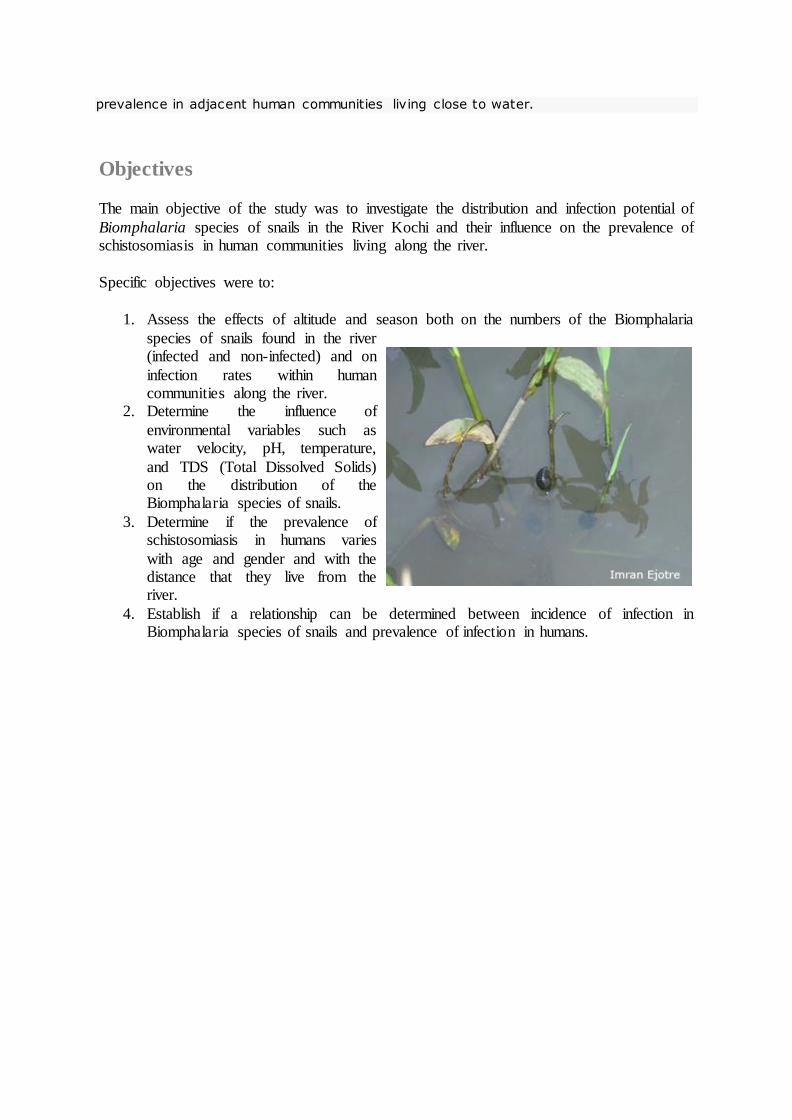
Objectives

The main objective of the study was to investigate the distribution and infection potential of

Biomphalaria species of snails in the River Kochi and their influence on the prevalence of schistosomiasis in human communities living along the river.

Specific objectives were to:

1. Assess the effects of altitude and season both on the numbers of the Biomphalaria

species of snails found in the river (infected and non-infected) and on

infection rates within human communities along the river.

2. Determine the influence of

environmental variables such as water velocity, pH, temperature,

and TDS (Total Dissolved Solids) on the distribution of the Biomphalaria species of snails.

3. Determine if the prevalence of schistosomiasis in humans varies

with age and gender and with the distance that they live from the river.

4. Establish if a relationship can be determined between incidence of infection in Biomphalaria species of snails and prevalence of infection in humans.

Questions to be addressed

This project is a fairly complicated study to address different aspects of schistosomiasis

infection. The different questions posed have already been listed under Objectives. As well as attempting to answer these questions we shall also be considering:

how well is the study designed to address the objectives; how well were the collected data managed to address the questions posed;

how should the analysis of the data be approached to tackle each of the objectives?

Study design

This MSc study was conducted along the River Kochi in the West Nile region of Uganda bordering the Democratic Republic of Congo.

This river crosses the region from its source near the border at an altitude of over 1,000 m above

sea level to the Albert Nile at about 600 m, and hence transcends a range of geographical conditions. Anecdotal evidence has suggested

that the prevalence of the disease increases as one travels westwards from the border.

Five sites were selected adjacent to the river

approximately 20 km apart. Points on the river marking the central positions of each community living at the sites were recorded by a GPS. Data

were collected from four families living within 3 km either side of this reference point. Data were

also collected from four families situated more than 3km away from the river to serve as controls.

Stool examinations were examined once a month from October 2007 to March 2008 for

Schistosoma mansoni eggs in each member of a family over the age of four years, except

where a family member had not consistently stayed in the family over the previous year. Bottles for collecting stool samples were distributed on a given day each month and families

notified that bottles should be ready for collection by 0800 hours the following morning. Each specimen bottle bore the site name, the number allocated to the family and the name,

age and the gender of the family member.

Areas for sampling the snails living in the river were also defined. These measured 30 m along the bank and 3 m into the main body of the water. The corners of these rectangular sampling areas were marked by pegs so that successive samplings could be performed across

the same area. Each site was sampled weekly from 0800 − 0900 hours over a period of six months.

All snails found floating or attached to vegetation were collected using a scooping net with a

long handle and placed on white plastic trays in order to be able to rapidly identify the different species. Snails of the Biomphalaria species, responsible for the transmission of

bilharzia, were transferred into large plastic buckets filled with water from the snail sampling areas and containing appropriate aquatic plants to simulate natural environmental conditions. These were taken to the field centre to screen for the microscopic presence of Schistosoma

mansoni cercariae. Snails that were not shedding cercariae were kept for a week to allow subsequent development of cercariae arising from early stages of infection.

Snails that did not shed cercariae in either screening were considered to be uninfected. These

and the other snail species were taken 1 km downstream and returned to the river. This was to maintain similar proportions of snails within the sampling areas and to avoid sampling the same snails on different sampling occasions.

Before sampling of snails began environmental variables thought to be responsible for

influencing the distribution of these snails along the river were also recorded. These included water flow velocity, water pH, water temperature and concentration of total dissolved solids

(TDS) in the water. Water flow velocity was obtained by sprinkling methyl orange dye from the upstream mark of the sampling area and recording the time taken for the dye colour to cover the 30 m distance to the downstream mark. Values for pH and temperature were

obtained by using a pH meter integrated with a temperature probe. TDS concentration was determined using a conductivity meter.

Source material

Three data sets are associated with this case study. CS14Data1 contains data on

measurements made at each site and each month in the river together with numbers of people sampled and numbers and percentages of samples found to be positive. Data

collected from the river include the numbers of different species of snails recorded each month including the number of Biomphalaria species responsible for the transmission of bilharzia together with numbers infected. Data for the environmental variables (water flow

velocity, pH, temperature and TDS) are also included in this file.

Three of the months (October, November and December) experienced heavy rains of above 900 mm and have been recorded as wet, whilst the other three months (January, February

and March) experienced little or no rains and have been recorded as dry.

Human data are contained in CS14Data2. Each record contains the numbers of individuals sampled and the number of samples found to be positive during the study, categorised by

site, distance from river, gender and age group: 5 − 9 years (regarded as children), 10 − 19 years (regarded as adolescents) and 20 years and above (regarded as adults). The average

percentage of samples per month found to be positive has also been calculated. Everyone was eager to participate in the study as it gave them an opportunity to know their monthly worm status, and there were few occasions when individuals missed an examination.

Data are documented in CS14Doc1 and CS14Doc2, respectively.

The third data set CS14Data3 is a subset of CS14Data1 derived to analyse associations between snail numbers and environmental variable measurements.

Data management

When preparing data recording sheets it is important to file them safely and to be able to visualise ahead how the data will be analysed. For a student tackling a research project this is not an easy task, and, as will be seen at the end of this data management section, mistakes

were made in this MSc project.

Recordings on snail counts and environmental variable values were initially entered into recording sheets as shown below. This is essentially as displayed in CS14Data1 except that

it would in hindsight have been better to record counts for the different snail species in different columns to ease the entry of data into the spread sheet. Otherwise, the layout of the sheet proved to be fine for analysis.

Recording of family data was more difficult to manage. Separate recording sheets were

prepared for each family as illustrated here.

Before any data recording begins it is important to decide how the collected data will be analysed. Consider Objective 3: to determine whether the

prevalence of schistosomiasis in humans varies with age or gender and with the distance of the

family from the river.

Recorded infection data are discrete (+ve or −ve) and likely to be analysed by a method for dealing

with counts or proportions such as logistic regression. It is therefore important to establish an appropriate observational unit for the analysis.

It helps to consider how the data are structured. The study takes the form of a cluster. Five

sites were initially identified, then two locations within each site (near and far from the river) and then four families within each location. Within each family three age categories

were defined and each individual was also classified by his/her gender. Each individual was then sampled once a month.

In order to answer Objective 3 set out on the previous page the monthly infection prevalence

data need to be characterised by age group, by gender and by distance from the river. If we ignore family and assume that village populations are fairly homogeneous, then we see that

the basic observational unit for analysis contains the sums of recorded negative and positive diagnoses in any one of the month x location x age group x gender subclasses. At the outset, therefore, it might have been sensible to prepare the recording sheet for each family with

members listed in age x gender group order so that the summations for each group can be done by hand and added to the recording sheets. A lot of time was spent entering the data for

each member of each family into a laptop; this proved not to be necessary as individual values were not used in the analysis.

The above table illustrates how total values for each family by location, age and gender and month might instead have been entered and stored into the computer. An additional column

has been added to the recording sheet to show, for example, how numbers of positive cases recorded over the period can also be calculated. Unfortunately, by the time it was realised

that the monthly information by age group and gender was needed as well as the total values, the individual recording sheets had been lost. Having entered the data into the

computer it is then necessary to sum up the results for the four families within each location to produce the data contained in CS14Data2, which represent the basic observational units

(see previous page) needed for the analysis. However, for the reasons mentioned above, only the numbers of positive test results recorded over the 6-month period are included in this

file, not the separate values for each month.

For comparisons involving river and human data (see Objective 4: establish if a relationship

can be determined between incidence of infection in snails and prevalence of infection in humans) total values summed over age and gender are required by site and month to match the river data stored in CS4Data1. Fortunately, these data had been calculated before the

recording sheets had been lost.

It is worth describing the difficulties that occurred in managing the data. Data were collected

from the three districts Koboko, Yumbe and Moyo which stretch over a distance of nearly 100 km. The senior author was based in the middle of these districts, namely Yumbe. He

was provided with a community office in Yumbe for him to handle his paper work and to keep some field equipment. None of the districts had access to electricity and so, after completing the monthly field recording sheets, he travelled to Arua in another district where

thermal power was available. Here he entered the data into his laptop.

The original recording sheets remained in a drawer in the Yumbe office. Later during the analysis for this case study he returned to Yumbe to collect the recording sheets only to find

that the community organisation had relocated itself and had discarded a lot of its paper work. His recording sheets were among these papers!! The author's supervisors worked 800 km in Mbale district in Eastern Uganda; during one of these trips to meet them his laptop

was stolen.

Although not all students will be expected to work under such difficult conditions as this, there are, nevertheless, many lessons to be learned. In particular, the case study emphasises

the need for young researchers to be taught necessary data management skills during their training. Fortunately the mistakes that occurred, i.e. not ensuring that the raw data sheets

were safely stored and not adequately backing up the computer data files, did not completely ruin this study and some potentially interesting results have been obtained.

Exploration and description

Altitude and season

The table (derived via Stats → Summary Statistics → Summaries of Groups

(Tabulation)...) applied to NBiom in CS14Data1 shows that no Biomphalaria species of snails were recorded during the wet season. During the dry season the numbers of snails

increased with decreasing altitude from none recorded at an altitude of 1189 m to a mean of 62 snails recorded per month at an altitude of 638 m or 639 m.

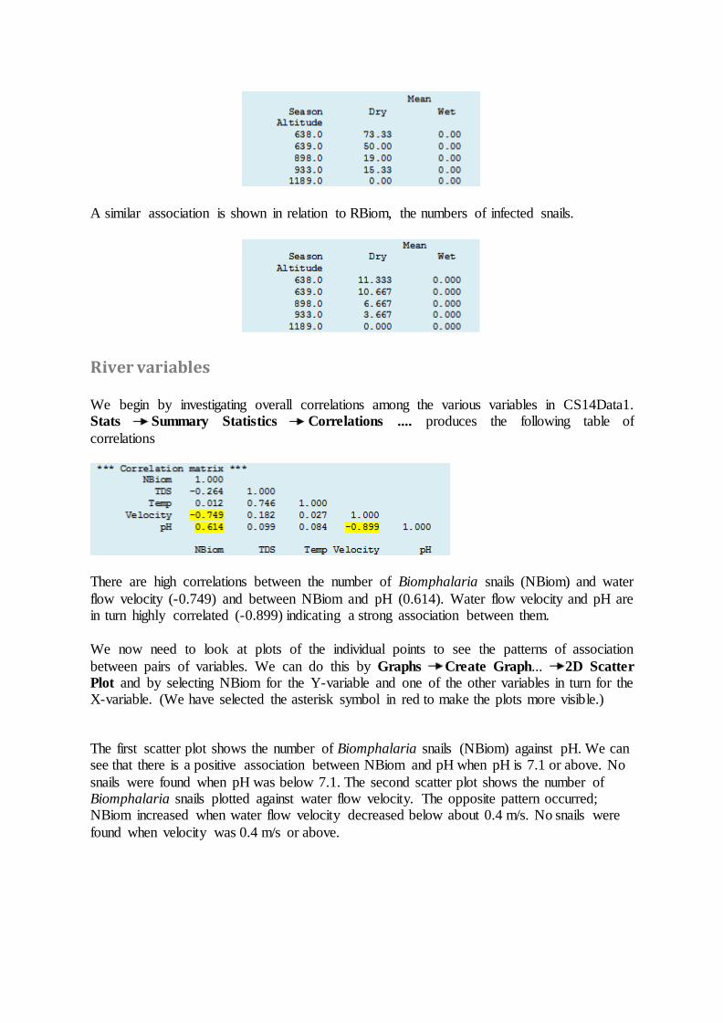
A similar association is shown in relation to RBiom, the numbers of infected snails.

River variables

We begin by investigating overall correlations among the various variables in CS14Data1. Stats Summary Statistics Correlations .... produces the following table of

correlations

There are high correlations between the number of Biomphalaria snails (NBiom) and water

flow velocity (-0.749) and between NBiom and pH (0.614). Water flow velocity and pH are in turn highly correlated (-0.899) indicating a strong association between them.

We now need to look at plots of the individual points to see the patterns of association

between pairs of variables. We can do this by Graphs Create Graph... 2D Scatter

Plot and by selecting NBiom for the Y-variable and one of the other variables in turn for the X-variable. (We have selected the asterisk symbol in red to make the plots more visible.)

The first scatter plot shows the number of Biomphalaria snails (NBiom) against pH. We can see that there is a positive association between NBiom and pH when pH is 7.1 or above. No

snails were found when pH was below 7.1. The second scatter plot shows the number of Biomphalaria snails plotted against water flow velocity. The opposite pattern occurred; NBiom increased when water flow velocity decreased below about 0.4 m/s. No snails were

found when velocity was 0.4 m/s or above.

We now need to compare water flow velocity and pH. The scatter plot shows that the two variables

are approximately linearly related. If we sort the data (Spread Sort...) into descending values of

velocity we can see, from the earlier graphs, that the velocity and pH values (approximately < 0.4 and > 7 m/s, respectively) that are associated with

changes in NBiom tend to be in records 17 to 30.

We shall save these records in CS14Data3 for subsequent regression analysis under Statistical modelling by selecting and deleting rows 1-16 (Spread Delete Selected rows).

In view of the result shown earlier that snail incidence is associated with altitude and season it is worth summarising mean values for water flow velocity and pH levels in the same way.

Thus, for water flow velocity we can see that snails were found only in the dry season at the

five sites where the velocity was in a range of 0.19 to 0.31 m/s. In Site 5 at the highest altitude, where no snails were found, the velocity in the dry season was 0.48 m/s, which is at

the lower end of the range of values shown for the wet season and above the value of 0.4 m/s (the upper limit for presence of snails quoted on the previous page).

A similar trend can be seen for pH. Snails were found only when pH values were 7.1 or above.

Human infections

We shall begin by summarising in two-way tables the average

percentage of individuals found to be infected each month, namely

P_infected (calculated from N_age_gen and N_infections). Using Stats

→ Summary Statistics → Summaries of

Groups (Tabulation)... we first obtain a table of means by age and site. Comparing

the overall site means we can see that less than 1% of samples per month were infected in Site 1, whereas between 4% and 5.3% of

people were infected per month in the other four sites. These latter values would appear to be too close to each other to be significantly different. Percentages in Age group 2 -

adolescents (5.2%) and in Age group 3 - adults (4.3%) were higher than in Age group 1 - children (2.4%).

The two-way table by age and gender indicates that fewer female children and

adolescents (Gender 2) tended to be infected than their male counterparts (Gender 1), but

that infection rates in adults were similar. The two-way table by age and location shows that distance from the river had little impact on disease prevalence.

We are now ready to fit models to the data (see Statistical modelling). Because hardly any

infection was detected in Site 1 we shall ignore this site and fit parameters for age and gender to the other four sites.

Snail and human infections

Percentages of humans infected each month at each site are contained in the variable Phum

contained in CS14Data1 alongside the river variables. Excluding Site 1 in which no snails were found, a scatter plot is shown alongside (achieved via Graphs Create Graph...

2D Scatter Plot) displaying the percentages of humans infected each month at each site against the corresponding numbers of Biomphalaria snails

found in the river.

It can be seen that as the number of snails increases there is a tendency for the numbers of humans

detected positive to increase too. This is especially the case in Site 4 and Site 5 where numbers of snails found during the dry season showed the

greatest increase. This indicates a potential link between increases in the population of snails down

river during the dry season and the incidence of new infections detected in humans.

There is little more that one can do with these data except investigate the monthly incidence of infections among individuals to see which ones were likely to be persistent and which

ones were likely to be new infections. Unfortunately, these data have been lost.

The graph shows the monthly prevalence levels to be somewhat low; this is puzzling in view of the endemic nature of the disease in the region. What has not been mentioned is that the

Government conducted a mass chemotherapy programme in the region a year earlier to de-worm communities. This is likely to have influenced the results of this study. Also not

everyone who is infected with bilharzia will show clinical signs.

Statistical modelling

River variables

We shall now explore further the associations

between number of Biomphalaria snails and

water flow velocity and pH measurements over the restricted range of

velocity and pH values stored in CS14Data3.

Using Stats →

Regression Analysis → Generalized Linear Models ... we can fit a linear regression model

with the two independent variables Velocity and pH.

From the output we can see that the regression mean square is highly significant (P<0.001) and that the model accounts for 80.5% of the variation in Biomphalaria numbers. This is

equivalent to a multiple correlation coefficient of 0.9 (square root of

0.805).

From the t-values for the parameter estimates it can be seen that both

independent variables contribute significantly to the equation (P<0.05). Another way of understanding this (see next page) is to click the Options... button in the Dialog Box and tick 'Accumulated'.

We can write the regression equation as NBiom = -1432 + 213(±82)pH -192(±63)Velocity

With 'Accumulated' ticked in

the dialog box an analysis of variance table is provided showing the effect of adding

independent variables one by one. Thus, inclusion of pH on

its own is highly significant (P<0.001) but addition of Velocity to the model is also significant (P<0.05). Note that the F value of 0.011 is the same as that for the t-value on the previous page; this demonstrates how the F test (with one degree of freedom in the

numerator) is analogous to the t test.

Changing the order in which

the independent variables are introduced results in this alternative version of the

analysis of variance table; this shows what happens when pH is added as the second variable.

A possible explanation for the association is that the river becomes wider and so the flow

speed of the water reduces further downstream. Stable water conditions downstream would be particularly prevalent during the dry season. Such conditions would enable the snails to anchor more easily on the water vegetation. Also, as the debris carried down the river settles

and rots down, so the pH of the water gradually increases. This would explain why higher numbers of Biomphalaria species of snails are associated with lower water flow rates and

higher pH levels.

Human infections

We first exclude Site 1 using Spread → Restrict/Filter → To Groups (factor levels)... and then analyse the variable P_infected. The data are balanced with three age groups, male and female in each of four sites so we could analyse the data using a randomised block model. However, we notice that separate

values of P_infected are based on different numbers of individuals; this

influences slightly the precision with which each P_infected value is determined. We shall, therefore, show

how the data can be analysed using a weighted analysis of variance.

We start by applying Stats →

Regression Analysis → Generalized

Linear Models... and including just age in the model. By clicking Options... and clicking 'Accumulated' and entering N_age_gen into the 'Weights: box' (see dialog box alongside) we

obtain an analysis of variance for age alone. We can then click Change Model in the original dialog box and add

gender to the model, and then repeat and add the interaction.

From the resulting analysis of variance we see that both age

and gender are significant, but not the interaction. We can

then click Change Model again and drop Age.Gender to return to the model with just the two parameters: age and gender.

We can see from the parameter estimates that both adolescents (Age 2:

P<0.001)) and adults (Age 3: P<0.05)) are more frequently infected than children. Likewise females (Gender 2)

are significantly less infected than males (P<0.05).

By using the Predict command in the dialog box

we can obtain mean value estimates for the three age groups, and by clicking Predict again obtain

means for males and females. We can conclude, therefore, that the rate of infection in adolescents and adults in sites 2 − 5 is approaching twice that

in children and that males were slightly more frequently infected than females, maybe because males spend more time working or playing in the river. The overall average

monthly detected percentage infection rate was, however, very low.

As shown earlier, schistosomiasis prevalence was higher in the overall population in the dry than the

wet season. However, data by age group and gender are no longer available to allow the data to

be separated in this way.

Findings, implications and lessons learned

A number of conclusions can be drawn from this study. Considering each of the four

objectives in turn:

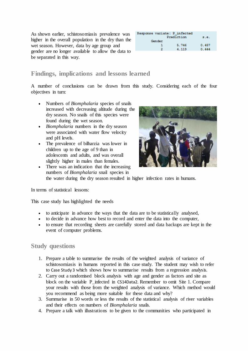
Numbers of Biomphalaria species of snails increased with decreasing altitude during the dry season. No snails of this species were

found during the wet season. Biomphalaria numbers in the dry season

were associated with water flow velocity and pH levels.

The prevalence of bilharzia was lower in

children up to the age of 9 than in adolescents and adults, and was overall

slightly higher in males than females. There was an indication that the increasing

numbers of Biomphalaria snail species in

the water during the dry season resulted in higher infection rates in humans.

In terms of statistical lessons:

This case study has highlighted the needs

to anticipate in advance the ways that the data are to be statistically analysed, to decide in advance how best to record and enter the data into the computer,

to ensure that recording sheets are carefully stored and data backups are kept in the event of computer problems.

Study questions

1. Prepare a table to summarise the results of the weighted analysis of variance of

schistosomiasis in humans reported in this case study. The student may wish to refer to Case Study 3 which shows how to summarise results from a regression analysis.

2. Carry out a randomised block analysis with age and gender as factors and site as

block on the variable P_infected in CS14Data2. Remember to omit Site 1. Compare your results with those from the weighted analysis of variance. Which method would

you recommend as being more suitable for these data and why? 3. Summarise in 50 words or less the results of the statistical analysis of river variables

and their effects on numbers of Biomphalaria snails. 4. Prepare a talk with illustrations to be given to the communities who participated in

the study to explain the results in a way that they would understand. 5. Assuming that the Government's mass chemotherapy programme that took place

during the year prior to this study resulted in much lower incidences of schistosomiasis than would normally have been the case, decide how you would

repeat the study and suggest any modifications to the design. 6. This study indicates a possible link between Biomphalaria snail numbers and

infection incidence in humans. Based on the information contained in this study and

the results obtained, design a new study which focuses just on this objective.

Study design

7. This project has produced some interesting results that might be interesting to follow up as well as the one proposed in question 6. Suggest another question that you feel

could usefully be followed up and prepare a project proposal to tackle this question. 8. Design data recording sheets for the project you have proposed in one of questions 5,

6 or 7 and write down your recommendations for data security. 9. Other species of snails were also collected (see CS14Data1). Summarise effects of

season and altitude for each of these species. Do they show the same trends with water velocity or pH as Biomphalaria species? If not, suggest from a biological point

of view why not. 10. Describe in layman's terms the meaning of the word 'odds'– see Appendix.

Further reading

Kabatereine, N. B., Brooker, S., Edridah, M, Tukahebwa, Francis Kazibwe and Ambrose W. Onapa (2004). Epidemiology and Geography of Schistosoma mansoni in Uganda:

Implications for planning Control. Tropical Medicine and International Health 9: 3 372 –380. Abstract

Kazibwe, F., B. Makanga, C. Rubaire-Akiki, J. Ouma, C. Kariuki, N.B. Kabatereine, M.

Booth, B.J. Vennervald, R.F Sturrock and J.R. Stothard (2006). Ecology of Biomphalaria (Gastropoda: Planorbidae) in Lake Albert, Western Uganda: Snail distribution, infections with schistosomes and temporal associations with environmental dynamics. Hydrobiologia

00: 1-12. Abstract

Van Der Werf M.J., de Vlas S.J., Brooker S. et al (2003). Quantification of Clinical Morbidity caused by schistosome infection in Sub-Saharan Africa. Acta Tropica 86: 125-

139. Abstract

Acknowledgments

The first author thanks the Islamic University Staff Development Committee for having

sponsored his MSc program which yielded this research project. He acknowledges the many people that contributed to this research including all the families that readily volunteered to provide stool samples. He is also grateful to Dr John Rowlands for his assistance in the

preparation of this case study and for suggesting ways in which the data could be best handled and analysed.

Appendix

Human infections

This case study provides an opportunity to demonstrate the method of logistic regression.

Let us pretend that N_infections represents, not the numbers of times infections that were

detected but, in an environment where schistosomiasis is highly prevalent, the number of individuals found to be infected. We assume that

the data follow a binomial distribution and fit a logistical model to the data for sites 2-5 just with

a single parameter for age. We do this by using Stats → Regression Analysis → Generalized Linear Models... and choosing the model for modelling binomial

proportions as shown in the dialog box.

By clicking the Options...

button and ticking 'Accumulated' we obtain the analysis of deviance shown

here. By checking the value of the residual deviance we can ascertain how well the residuals follow a binomial

distribution. If the mean deviance approximates to 1, as can be seen here, the residual values can be assumed to follow a binomial distribution; the statistical significance of the change in deviance due to the inclusion of age can then be assumed to follow a Chi squared

distribution, shown here to be significant (P<0.01). If the mean deviance is much greater than 1 then the data are said to be over dispersed and an F test is required. (Note that this

interpretation does not apply when data comprise (0,1) values, i.e. not (r,n) values as used in this example.) The reader is referred to the guide on Statistical Modelling for further discussion on this topic.

Now we add gender to the model. We can click

Change Model... at the bottom right of the dialog box, enter Gender under

'Terms' in the new dialog box and click Add. We see

that addition of Gender to the model is significant (P<0.05).

By repeating the steps above and adding the term Age.

Gender we see that the interaction is not statistically

significant, so we can drop the interaction.

Parameter estimates

included in the output for the model with age and

gender are shown here. These are expressed relative to the baseline

levels of zero for Age 1 and Gender 1. Thus, the estimate for Age 2 is 0.921 higher and that for Age 3 is 0.655 higher than for Age 1. These differences are significant (P<0.01) and

(P<0.05), respectively. From the sizes of the standard errors we can detect that there is no significant difference between age groups 2 and 3. The parameter estimate for Gender 2 (females) is 0.485 lower than that for Gender 1 (P<0.05).

It is possible also to obtain estimates on

the original observational scale by clicking the Predict button at the

bottom right of the dialog box shown earlier. By then clicking 'Age' the table alongside is produced. This gives predicted estimates for the three age groups adjusted for

differences between males and females. Thus, 19% of children were found to be infected with bilharzia compared with an average of 34% in adolescents and adults.

Then, by clicking 'Gender' we see that

34% of males were found to be infected compared with 25% of females. Please note that this is a purely imaginary

interpretation of the values of the variable N_infections that have been simply used to illustrate the method of logistic regression. The results are not applicable to the case study.

The results of this analysis can be presented as shown in the table below; this is set out in the way recommended in the Reporting Guide. The numbers of individuals shown to be sampled and infected can be found via Stats → Summary Statistics → Summaries of Groups

(Tabulation).... and clicking 'Totals' in the dialog box for N_age_gen and N_infections, respectively. Inclusion of these raw values in the table is useful; they show the size of the

study so that the reader can appreciate the practical significance of the statistical conclusions drawn. Table: Effect of age and gender on infection rates of schistosomiasis in people living in villages along the River Kochi

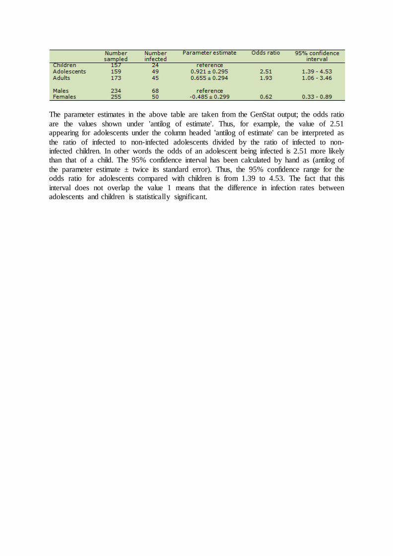
The parameter estimates in the above table are taken from the GenStat output; the odds ratio

are the values shown under 'antilog of estimate'. Thus, for example, the value of 2.51 appearing for adolescents under the column headed 'antilog of estimate' can be interpreted as

the ratio of infected to non-infected adolescents divided by the ratio of infected to non-infected children. In other words the odds of an adolescent being infected is 2.51 more likely than that of a child. The 95% confidence interval has been calculated by hand as (antilog of

the parameter estimate ± twice its standard error). Thus, the 95% confidence range for the odds ratio for adolescents compared with children is from 1.39 to 4.53. The fact that this

interval does not overlap the value 1 means that the difference in infection rates between adolescents and children is statistically significant.