CASE Network Report 41 - Currency Crises in Emerging Markets - Selected Comparative Studies
146
Marek D¹browski (ed.) Warsaw, 2001 No. 41 Currency Crises in Emerging Markets – Selected Comparative Studies
-
Upload
case-center-for-social-and-economic-research -
Category
Economy & Finance
-
view
422 -
download
5
description
This volume presents seven comparative studies of currency crises, which happened in the decade of 1990s in Latin America, South East Asia and in transition countries of Eastern Europe and the former USSR. Authored by: Rafal Antczak, Monika Blaszkiewicz, Marek Dabrowski, Malgorzata Jakubiak, Malgorzata Markiewicz, Wojciech Paczynski, Artur Radziwill, Marcin Sasin, Mateusz Szczurek Published in 2001
Transcript of CASE Network Report 41 - Currency Crises in Emerging Markets - Selected Comparative Studies

M a r e k D ¹ b r o w s k i ( e d . )
WW aa rr ss aa ww ,, 22 00 00 11 NNoo.. 4411
Currency Crises
in Emerging Markets
– Selected Comparative
Studies
The views and opinions expressed in this publication reflectAuthors’ point of view and not necessarily those of CASE.
Materials prepared for the conference summing up theresearch project No. 0144/H02/99/17 entitled "Analizaprzyczyn i przebiegu kryzysów walutowych w krajach Azji,Ameryki £aciñskiej i Europy Œrodkowo-Wschodniej: wnios-ki dla Polski i innych krajów transformuj¹cych siê" (Analysisof the Causes and Progress of Currency Crises in Asian,Latin American and CEE Countries: Conclusions for Polandand Other Transition Countries) financed by the StateCommittee for Scientific Research (KBN) in the years1999-2001.
The publication was financed by KBN and WestdeutscheLandesbank Polska S.A.
Key words: financial crises, currency crises, IMF, financialsystems, exchange rate regime, transition economies
DTP: CeDeWu Sp. z o.o.
Graphic Design – Agnieszka Natalia Bury
© CASE – Center for Social and Economic Research, Warsaw 2001
All rights reserved. No part of this publication may bereproduced, stored in a retrieval system, or transmitted in anyform or by any means, without prior permission in writingfrom the author and the CASE Foundation.
ISSN 1506-1647 ISBN 83-7178-259-4
Publisher:CASE – Center for Social and Economic Research ul. Sienkiewicza 12, 00-944 Warsaw, Polande-mail: [email protected]://www.case.com.pl

3
Currency Crises in Emerging Markets – Selected Comparative ...
CASE Reports No. 41
Contents
Introduction - Marek D¹browski . . . . . . . . . . . . . . . . . . . . . . . . . . . . . . . . . . . . . . . . . . . . . . . . . . . . .7
Part I. The Importance of the Real Exchange Rate Overvaluation and the Current Account Deficitin the Emergence of Financial Crises - Marcin Sasin . . . . . . . . . . . . . . . . . . . . . . . . . . . . . . . . . . . . . .91.1. Introduction . . . . . . . . . . . . . . . . . . . . . . . . . . . . . . . . . . . . . . . . . . . . . . . . . . . . . . . . . . . . . . . . . . . . . . . .91.2. Overvaluation . . . . . . . . . . . . . . . . . . . . . . . . . . . . . . . . . . . . . . . . . . . . . . . . . . . . . . . . . . . . . . . . . . . . . . .9
1.2.1. Theory . . . . . . . . . . . . . . . . . . . . . . . . . . . . . . . . . . . . . . . . . . . . . . . . . . . . . . . . . . . . . . . . . . . . . .91.2.2. How to Calculate a Real Exchange Rate . . . . . . . . . . . . . . . . . . . . . . . . . . . . . . . . . . . . . . . . . . . .101.2.3. Overvaluation and Currency Crises, an Empirical Evidence . . . . . . . . . . . . . . . . . . . . . . . . . . . . . .111.2.4. Trade-link Contagion: Competitive Devaluations . . . . . . . . . . . . . . . . . . . . . . . . . . . . . . . . . . . . . .13
1.3. Current Account . . . . . . . . . . . . . . . . . . . . . . . . . . . . . . . . . . . . . . . . . . . . . . . . . . . . . . . . . . . . . . . . . . . .141.3.1. Evolution of the Point of View on the Current Account . . . . . . . . . . . . . . . . . . . . . . . . . . . . . . . .14
1.3.1.1. The Early Views: the Trade/Elasticity Approach . . . . . . . . . . . . . . . . . . . . . . . . . . . . . . . .141.3.1.2. Intertemporal Approach: the Irrelevance of the Current Account Deficit
and the Lawson Doctrine . . . . . . . . . . . . . . . . . . . . . . . . . . . . . . . . . . . . . . . . . . . . . . .141.3.1.3. Surge in Capital Inflows: from the 5% Rule of Thumb to "Current Account Sustainability"15
1.3.2. Models of the Current Account . . . . . . . . . . . . . . . . . . . . . . . . . . . . . . . . . . . . . . . . . . . . . . . . . .161.3.2.1. Exchange Rate and Elasticity Approach . . . . . . . . . . . . . . . . . . . . . . . . . . . . . . . . . . . . . .161.3.2.2. Portfolio Approach . . . . . . . . . . . . . . . . . . . . . . . . . . . . . . . . . . . . . . . . . . . . . . . . . . . .161.3.2.3. Intertemporal Choice Approach . . . . . . . . . . . . . . . . . . . . . . . . . . . . . . . . . . . . . . . . . . .17
1.3.3. How to Calculate A Sustainable Current Account Deficit . . . . . . . . . . . . . . . . . . . . . . . . . . . . . . .191.3.3.1. Underlying Current Account Balance . . . . . . . . . . . . . . . . . . . . . . . . . . . . . . . . . . . . . . .191.3.3.2. Model-based Calculations . . . . . . . . . . . . . . . . . . . . . . . . . . . . . . . . . . . . . . . . . . . . . . . .191.3.3.3. Different Method for Different Types of Economies . . . . . . . . . . . . . . . . . . . . . . . . . . . .21
1.3.4. Empirical Evidence . . . . . . . . . . . . . . . . . . . . . . . . . . . . . . . . . . . . . . . . . . . . . . . . . . . . . . . . . . . .221.3.4.1. Determinants of Current Account and its Empirical Distribution over Time
and Countries . . . . . . . . . . . . . . . . . . . . . . . . . . . . . . . . . . . . . . . . . . . . . . . . . . . . . . . . .221.3.4.2. The Links Between Current Account and Crises . . . . . . . . . . . . . . . . . . . . . . . . . . . . . . .22
1.4. Conclusions . . . . . . . . . . . . . . . . . . . . . . . . . . . . . . . . . . . . . . . . . . . . . . . . . . . . . . . . . . . . . . . . . . . . . . .25References . . . . . . . . . . . . . . . . . . . . . . . . . . . . . . . . . . . . . . . . . . . . . . . . . . . . . . . . . . . . . . . . . . . . . . . . . .26
Part II. Choice of Exchange Rate Regime and Currency Crashes - Evidence of some Emerging Economies - Ma³gorzata Jakubiak . . . . . . . . . . . . . . . . . . . . . . . . . . . . . . . . . . . . . . . . . . . . . . . . . . . .292.1. Introduction . . . . . . . . . . . . . . . . . . . . . . . . . . . . . . . . . . . . . . . . . . . . . . . . . . . . . . . . . . . . . . . . . . . . . . .292.2. Old Dilemma: Fixed or Flexible? . . . . . . . . . . . . . . . . . . . . . . . . . . . . . . . . . . . . . . . . . . . . . . . . . . . . . . . .292.3. Costs of a Sudden Shift to a More Flexible Arrangement . . . . . . . . . . . . . . . . . . . . . . . . . . . . . . . . . . . . . .302.4. Why Emerging Markets Peg Their Currencies . . . . . . . . . . . . . . . . . . . . . . . . . . . . . . . . . . . . . . . . . . . . . .312.5. Choices Faced After a Currency Collapse . . . . . . . . . . . . . . . . . . . . . . . . . . . . . . . . . . . . . . . . . . . . . . . . .322.6. Empirical Evidence - Case Studies . . . . . . . . . . . . . . . . . . . . . . . . . . . . . . . . . . . . . . . . . . . . . . . . . . . . . . .32
2.6.1. Group First - Hard Pegs: Brazil, Thailand, Mexico . . . . . . . . . . . . . . . . . . . . . . . . . . . . . . . . . . . . .332.6.2. Group Second - Moderate Pegs: Russia, Georgia, Ukraine, Korea, Indonesia,
Malaysia, Moldova . . . . . . . . . . . . . . . . . . . . . . . . . . . . . . . . . . . . . . . . . . . . . . . . . . . . . . . . . . . . .35
4
Marek D¹browski (ed.)
2.6.3. Group Third - Floats: Kyrgyz Republic, Czech Republic, Bulgaria . . . . . . . . . . . . . . . . . . . . . . . . .392.6.4. Currency Board: Argentina in 1995 . . . . . . . . . . . . . . . . . . . . . . . . . . . . . . . . . . . . . . . . . . . . . . .41
2.7. Probability of Ending a Peg. Logit Estimation . . . . . . . . . . . . . . . . . . . . . . . . . . . . . . . . . . . . . . . . . . . . . . .412.8. Conclusions . . . . . . . . . . . . . . . . . . . . . . . . . . . . . . . . . . . . . . . . . . . . . . . . . . . . . . . . . . . . . . . . . . . . . . .42Appendix: Crisis Dates . . . . . . . . . . . . . . . . . . . . . . . . . . . . . . . . . . . . . . . . . . . . . . . . . . . . . . . . . . . . . . . . . . .44References . . . . . . . . . . . . . . . . . . . . . . . . . . . . . . . . . . . . . . . . . . . . . . . . . . . . . . . . . . . . . . . . . . . . . . . . . .45
Part III. International Liquidity, and the Cost of Currency Crises - Mateusz Szczurek . . . . . . . . . . . .473.1. Introduction . . . . . . . . . . . . . . . . . . . . . . . . . . . . . . . . . . . . . . . . . . . . . . . . . . . . . . . . . . . . . . . . . . . . . . .473.2. Foreign Exchange Reserves in Crisis Models . . . . . . . . . . . . . . . . . . . . . . . . . . . . . . . . . . . . . . . . . . . . . . .48
3.2.1. A Survey of Literature . . . . . . . . . . . . . . . . . . . . . . . . . . . . . . . . . . . . . . . . . . . . . . . . . . . . . . . . .483.2.2. A Survey of Empirical Results . . . . . . . . . . . . . . . . . . . . . . . . . . . . . . . . . . . . . . . . . . . . . . . . . . . .50
3.3. International Liquidity: Simple Model . . . . . . . . . . . . . . . . . . . . . . . . . . . . . . . . . . . . . . . . . . . . . . . . . . . . .523.3.1. Crisis and its Cost . . . . . . . . . . . . . . . . . . . . . . . . . . . . . . . . . . . . . . . . . . . . . . . . . . . . . . . . . . . .523.3.2. International Liquidity and its Cost . . . . . . . . . . . . . . . . . . . . . . . . . . . . . . . . . . . . . . . . . . . . . . . .543.3.3. Optimisation Problem . . . . . . . . . . . . . . . . . . . . . . . . . . . . . . . . . . . . . . . . . . . . . . . . . . . . . . . . .55
3.4. Empirical Application . . . . . . . . . . . . . . . . . . . . . . . . . . . . . . . . . . . . . . . . . . . . . . . . . . . . . . . . . . . . . . . . .563.4.1. Data . . . . . . . . . . . . . . . . . . . . . . . . . . . . . . . . . . . . . . . . . . . . . . . . . . . . . . . . . . . . . . . . . . . . . . .563.4.2. The Results . . . . . . . . . . . . . . . . . . . . . . . . . . . . . . . . . . . . . . . . . . . . . . . . . . . . . . . . . . . . . . . . .563.4.3. How Much the Policy Makers Fear the Crisis . . . . . . . . . . . . . . . . . . . . . . . . . . . . . . . . . . . . . . . .58
3.5. Conclusions . . . . . . . . . . . . . . . . . . . . . . . . . . . . . . . . . . . . . . . . . . . . . . . . . . . . . . . . . . . . . . . . . . . . . . .60Appendix . . . . . . . . . . . . . . . . . . . . . . . . . . . . . . . . . . . . . . . . . . . . . . . . . . . . . . . . . . . . . . . . . . . . . . . . . .60References . . . . . . . . . . . . . . . . . . . . . . . . . . . . . . . . . . . . . . . . . . . . . . . . . . . . . . . . . . . . . . . . . . . . . . . . . .61
Part IV. Financial Systems, Financial Crises, Currency Crises – Marcin Sasin . . . . . . . . . . . . . . . . . . .634.1. Introduction . . . . . . . . . . . . . . . . . . . . . . . . . . . . . . . . . . . . . . . . . . . . . . . . . . . . . . . . . . . . . . . . . . . . . . .634.2. Theoretical Aspects of Banking and Financial Crises . . . . . . . . . . . . . . . . . . . . . . . . . . . . . . . . . . . . . . . . .634.2.1. Definitions . . . . . . . . . . . . . . . . . . . . . . . . . . . . . . . . . . . . . . . . . . . . . . . . . . . . . . . . . . . . . . . . . . . . . .63
4.2.2. The Relationship between Banking and Currency Crises . . . . . . . . . . . . . . . . . . . . . . . . . . . . . . .644.2.3. The Theory and Practice of a Banking System Crisis . . . . . . . . . . . . . . . . . . . . . . . . . . . . . . . . . . .64
4.3. Assessing the Condition of a Banking System . . . . . . . . . . . . . . . . . . . . . . . . . . . . . . . . . . . . . . . . . . . . . . .714.4. Empirical Evidence and the Determinants of Banking and Currency Crises . . . . . . . . . . . . . . . . . . . . . . . .72
4.4.1. Banking Crises in the Real World . . . . . . . . . . . . . . . . . . . . . . . . . . . . . . . . . . . . . . . . . . . . . . . . .724.4.2. Some Statistics Concerning Banking, Currency and Twin Crisis . . . . . . . . . . . . . . . . . . . . . . . . . . .744.4.3. The Determinants of Banking Crises . . . . . . . . . . . . . . . . . . . . . . . . . . . . . . . . . . . . . . . . . . . . . . .754.4.4. The Empirical Evidence on the Interrelation between Currency and Banking Crises . . . . . . . . . . .76
4.5. Conclusions . . . . . . . . . . . . . . . . . . . . . . . . . . . . . . . . . . . . . . . . . . . . . . . . . . . . . . . . . . . . . . . . . . . . . . .77References . . . . . . . . . . . . . . . . . . . . . . . . . . . . . . . . . . . . . . . . . . . . . . . . . . . . . . . . . . . . . . . . . . . . . . . . . .78
Part V. Propagation of Currency Crises – The Case of the Russian Crisis£ukasz Rawdanowicz . . . . . . . . . . . . . . . . . . . . . . . . . . . . . . . . . . . . . . . . . . . . . . . . . . . . . . . . . . . . . .795.1. Introduction . . . . . . . . . . . . . . . . . . . . . . . . . . . . . . . . . . . . . . . . . . . . . . . . . . . . . . . . . . . . . . . . . . . . . . .795.2. Definitions of Contagion . . . . . . . . . . . . . . . . . . . . . . . . . . . . . . . . . . . . . . . . . . . . . . . . . . . . . . . . . . . . . .805.3. The Channels of Crises Propagation . . . . . . . . . . . . . . . . . . . . . . . . . . . . . . . . . . . . . . . . . . . . . . . . . . . . .805.4. Measuring Crises Propagation . . . . . . . . . . . . . . . . . . . . . . . . . . . . . . . . . . . . . . . . . . . . . . . . . . . . . . . . . .82
CASE Reports No. 41
5
Currency Crises in Emerging Markets – Selected Comparative ...
CASE Reports No. 41
5.4.1. Cross-Market Correlation Coefficients . . . . . . . . . . . . . . . . . . . . . . . . . . . . . . . . . . . . . . . . . . . . .825.4.2. Limited Dependent Variable Models . . . . . . . . . . . . . . . . . . . . . . . . . . . . . . . . . . . . . . . . . . . . . . .82
5.5. Model . . . . . . . . . . . . . . . . . . . . . . . . . . . . . . . . . . . . . . . . . . . . . . . . . . . . . . . . . . . . . . . . . . . . . . . . . .835.5.1. Definition of a Crisis . . . . . . . . . . . . . . . . . . . . . . . . . . . . . . . . . . . . . . . . . . . . . . . . . . . . . . . . . . .835.5.2. The Russian Crisis – Stylised Facts . . . . . . . . . . . . . . . . . . . . . . . . . . . . . . . . . . . . . . . . . . . . . . . .845.5.3. The Probit Model . . . . . . . . . . . . . . . . . . . . . . . . . . . . . . . . . . . . . . . . . . . . . . . . . . . . . . . . . . . . .885.5.4. The Balance of Payments Model . . . . . . . . . . . . . . . . . . . . . . . . . . . . . . . . . . . . . . . . . . . . . . . . . .89
5.6. Conclusions . . . . . . . . . . . . . . . . . . . . . . . . . . . . . . . . . . . . . . . . . . . . . . . . . . . . . . . . . . . . . . . . . . . . . . .93Appendix . . . . . . . . . . . . . . . . . . . . . . . . . . . . . . . . . . . . . . . . . . . . . . . . . . . . . . . . . . . . . . . . . . . . . . . . . .95References . . . . . . . . . . . . . . . . . . . . . . . . . . . . . . . . . . . . . . . . . . . . . . . . . . . . . . . . . . . . . . . . . . . . . . . . .100
Part VI. The Economic and Social Consequences of Financial CrisesMonika B³aszkiewicz, Wojciech PaczyñskiPart VI. The Economic and Social Consequences of Financial Crises - Monika B³aszkiewicz, Wojciech Paczyñski1036.1. Introduction . . . . . . . . . . . . . . . . . . . . . . . . . . . . . . . . . . . . . . . . . . . . . . . . . . . . . . . . . . . . . . . . . . . . . .1036.2. Review of the Literature . . . . . . . . . . . . . . . . . . . . . . . . . . . . . . . . . . . . . . . . . . . . . . . . . . . . . . . . . . . .1046.3. Some Statistical Exercises . . . . . . . . . . . . . . . . . . . . . . . . . . . . . . . . . . . . . . . . . . . . . . . . . . . . . . . . . . . .1046.3.1. The Definition of a Crisis . . . . . . . . . . . . . . . . . . . . . . . . . . . . . . . . . . . . . . . . . . . . . . . . . . . . . . . . . . .1046.3.2. The Sample . . . . . . . . . . . . . . . . . . . . . . . . . . . . . . . . . . . . . . . . . . . . . . . . . . . . . . . . . . . . . . . . . . . . .1056.3.3. Data . . . . . . . . . . . . . . . . . . . . . . . . . . . . . . . . . . . . . . . . . . . . . . . . . . . . . . . . . . . . . . . . . . . . . . . . .1056.3.4. Economic Performance Before and After the Crisis . . . . . . . . . . . . . . . . . . . . . . . . . . . . . . . . . . . . . . .1056.4. The Cost of a Crisis . . . . . . . . . . . . . . . . . . . . . . . . . . . . . . . . . . . . . . . . . . . . . . . . . . . . . . . . . . . . . . . .1166.5. Turning Crisis into Opportunity? Do Crises Bring Catharisis to Economies? . . . . . . . . . . . . . . . . . . . . . . .1186.6. Conclusions . . . . . . . . . . . . . . . . . . . . . . . . . . . . . . . . . . . . . . . . . . . . . . . . . . . . . . . . . . . . . . . . . . . . . .119Appendix. The Definition of a Crisis . . . . . . . . . . . . . . . . . . . . . . . . . . . . . . . . . . . . . . . . . . . . . . . . . . . . . . . .120References . . . . . . . . . . . . . . . . . . . . . . . . . . . . . . . . . . . . . . . . . . . . . . . . . . . . . . . . . . . . . . . . . . . . . . . . .121
Part VII. Part VII. Financial Crises in FSU Countries: The Role of the IMFRafa³ Antczak, Ma³gorzata Markiewicz, Artur Radziwi³³ . . . . . . . . . . . . . . . . . . . . . . . . . . . . . . . . . . .1237.1. Introduction . . . . . . . . . . . . . . . . . . . . . . . . . . . . . . . . . . . . . . . . . . . . . . . . . . . . . . . . . . . . . . . . . . . . . .1237.2. The Nature of Financial Crisis in FSU Countries . . . . . . . . . . . . . . . . . . . . . . . . . . . . . . . . . . . . . . . . . . .1247.3. The Role of the IMF . . . . . . . . . . . . . . . . . . . . . . . . . . . . . . . . . . . . . . . . . . . . . . . . . . . . . . . . . . . . . . . .1267.4. IMF Programs in FSU Countries . . . . . . . . . . . . . . . . . . . . . . . . . . . . . . . . . . . . . . . . . . . . . . . . . . . . . . .1297.5. Program Deficiencies and Consequences . . . . . . . . . . . . . . . . . . . . . . . . . . . . . . . . . . . . . . . . . . . . . . . .131
7.5.1. Growth Assumptions . . . . . . . . . . . . . . . . . . . . . . . . . . . . . . . . . . . . . . . . . . . . . . . . . . . . . . . . .1317.5.2. Fiscal Policy and Sustainability of Programs . . . . . . . . . . . . . . . . . . . . . . . . . . . . . . . . . . . . . . . . .1317.5.3. Myopia in Action . . . . . . . . . . . . . . . . . . . . . . . . . . . . . . . . . . . . . . . . . . . . . . . . . . . . . . . . . . . .1357.5.4. Weak Conditionality . . . . . . . . . . . . . . . . . . . . . . . . . . . . . . . . . . . . . . . . . . . . . . . . . . . . . . . . . .1397.5.5. Soft Financing . . . . . . . . . . . . . . . . . . . . . . . . . . . . . . . . . . . . . . . . . . . . . . . . . . . . . . . . . . . . . . .145
7.6. Conclusions: Political and Institutional Considerations . . . . . . . . . . . . . . . . . . . . . . . . . . . . . . . . . . . . . . .147

6
Marek D¹browski (ed.)
CASE Reports No. 41
Marek D¹browski
Marek D¹browski, Professor of Economics, V-Chairman and one of the founders of the CASE – Center for Social and Eco-nomic Research in Warsaw; Director of the USAID Ukraine Macroeconomic Policy Program in Kiev carried out by CASE;from 1991 involved in policy advising for governments and central banks of Russia, Ukraine, Kyrgyzstan, Kazakhstan, Geor-gia, Uzbekistan, Mongolia, and Romania; 1989–1990 First Deputy Minister of Finance of Poland; 1991–1993 Member of theSejm (lower house of the Polish Parliament); 1991–1996 Chairman of the Council of Ownership Changes, the advisory bodyto the Prime Minister of Poland; 1994–1995 visiting consultant of the World Bank, Policy Research Department; from 1998Member of the Monetary Policy Council of the National Bank of Poland. Recently his area of research interest is concen-trated on macroeconomic policy problems and political economy of transition.
Rafa³ Antczak
Rafa³ Antczak is an economist at the Center for Social and Economic Reasearch. The advisor to: the government of Ukraineand National Bank of Ukraine in 1994–1998, the government of the Kyrgyz Republic in 1995, and the President of Kaza-khstan in 1995. The research activities included also visits to Russia and Belarus. The main areas of activity combine macro-economic problems of transformation, monetary policy, and foreign trade.
Monika B³aszkiewicz
The author received MA in International Economics from the University of Sussex, UK ( 2000) and the Department of Eco-nomics at the University of Warsaw (2001). Presently, Monika B³aszkiewicz works for the Ministry of Finance at the Depart-ment of Financial Policy, Analysis and Statistics. Her main interest lies in short-term capital flows to developing and emerg-ing market economies and the role this kind of capital plays in the process of development and integration with the globaleconomy. In every day work she deals with the problem related to Polish integration with EU, in particular in the area ofEconomic and Monetary Union.
Ma³gorzata Jakubiak
Ma³gorzata Jakubiak has collaborated with the CASE Foundation since 1997. She graduated from the University of Sussex,UK (1997) and the Department of Economics at the University of Warsaw (1998). Her main areas of interest include for-eign trade and macroeconomics of open economy. She has published articles on trade flows, exchange rates, savings andinvestments in Poland and other CEE countries. During 2000–2001 she was working at the CASE mission in Ukraine as res-ident consultant.
Ma³gorzata Markiewicz
Ma³gorzata Markiewicz graduated from the Department of Economics at the Warsaw University. She has collaborated withthe CASE Foundation since 1995. She participated in advisory projects in Kyrgyzstan (1996, 1997), Georgia (1997) andUkraine (1995, 1998–2000). She has been an advisor to government and central bank representatives. Her main areas ofinterest include macroeconomic policies with a special emphasis put on fiscal problems and the correlation between fiscaland monetary policies.
7
Currency Crises in Emerging Markets – Selected Comparative ...
CASE Reports No. 41
Wojciech Paczyñski
Economist at the Centre for Eastern Studies, Ministry of Economy, Warsaw.Graduated from the University of Sussex (1998, MA in International Economics) and University of Warsaw (1999, MA inEconomics; 2000, MSc in Mathematics). Since 1998 he has been working as an economist at the CES. In 2000 started co-operation with CASE. His research interest include economies in transition, political economy and game theory.
Artur Radziwi³³
Artur Radziwi³³ is a researcher at the Center for Social and Economic Research (CASE) and a junior expert at the Interna-tional Economic Advisory Group in Moldova. He obtained his undergraduate education within the Columbia University Pro-gram. He received his MA in Economics at Sussex University, UK and at Warsaw University (summa cum laude).
£ukasz Rawdanowicz
£ukasz Rawdanowicz graduated from Sussex University in 1998 (MA in International Economics) and Warsaw University –Department of Economics in 1999 (MA in quantitative methods). His main area of interest is econometrics and macroeco-nomics (in particular issues on international economics, foreign trade, balance of payments, and forecasting). He is a co-author and editorial assistant of the quarterly bulletins Polish Economic Outlook and Global Economy. He was also involvedin the project on the development of a macro-model in the Kyrgyz Republic.
Marcin Sasin
Marcin Sasin has joined CASE Foundation in 2000. He is an economist specializing in international financial economics andmonetary policy issues. He obtained Master of Science at the Catholic University of Leuven, Belgium in 2000. He also holdsMA in Oriental Studies at the Warsaw University.
Mateusz Szczurek
Mateusz Szczurek is an economist at ING Barings covering Polish macroeconomics and fixed income analysis. He is also aPhD student at the University of Sussex, preparing the thesis on international liquidity and foreign exchange crises. He holdsMA in international economics from the University of Sussex, MA ineconomics from the University of Warsaw, as well as BA joint honours degree from Columbia University and Warsaw Uni-versity. He is a member of Polish Society of Market Economists, Polish Association of Business Economists, and the presi-dent of University of Sussex Polish Alumni group.
8
Marek D¹browski (ed.)
CASE Reports No. 41
This volume presents seven comparative studies of cur-rency crises, which happened in the decade of 1990s in LatinAmerica, South East Asia and in transition countries of East-ern Europe and the former USSR. All the studies were pre-pared under the research project no. OI44/H02/99/17 on"Analysis of Currency Crises in Countries of Asia, LatinAmerica and Central and Eastern Europe: Lessons forPoland and Other Transition Countries", carried out byCASE and financed by the Committee for ScientificResearch (KBN) in the years 1999–2001. They will be sub-jects of public presentation and discussion during the semi-nar in Warsaw organized by CASE on June 28, 2001, underthe same research project. This is a continuation of twoother issues of CASE Reports containing eleven countries'monographs related to currency crises episodes in thesethree regions and a couple of other comparative studiespublished in the CASE Studies and Analyzes series.
Three first studies in this volume deal with broad issueof current account, exchange rate and international reservesof a central bank.
Marcin Sasin discusses the importance of the realexchange rate overvaluation and the current account deficit,which are usually considered as the main causes of currencycrises. While generally confirming the importance of the firstfactor, author shows that question of sustainability of currentaccount deficit has a very individual country characteristic.
The next analysis of Ma³gorzata Jakubiak concerns thechoice of exchange rate regimes from the point of view ofboth avoiding and efficient managing currency crises. Authorcompares advantages and disadvantages of the fixed versusfloating exchange rate regimes from the point of view ofcredibility of monetary policies, preventing currency crisisand coping with its consequences. She demonstrates, basingon an empirical analysis, that the most costly are changes ofexchange rate regimes (usually abandoning the peg) underthe pressure of speculative attack.
Mateusz Szczurek provides the additional insight to thisdiscussion estimating the size of optimal international liquid-ity taking into consideration potential costs of the crisis, onthe one hand, and costs of maintaining the internationalreserves, on the other.
The next study concerns interrelations between bankingand currency crises basing on extensive review of an eco-nomic literature. Marcin Sasin analyzes the institutional andstructural sources of instability of the banking sector inemerging markets. One of them is the direct and indirectvulnerability of banks in relation to sudden interest rate andexchange rate changes. On the other hand, collapse of thesome big banks must lead to credibility crisis of a domesticcurrency.
Lukasz Rawdanowicz addresses another hot issue in theeconomic debates of the last decade, i.e. contagion effect ofa crisis in one country on the macroeconomic stability of itsclose and more distant neighbors. He analyzes the impact ofthe Russian 1998 crisis on the situation of CIS countries tak-ing into consideration both trade and financial channels.
Monika B³aszkiewicz and Wojciech Paczyñski try toassess the economic and social consequences of currencycrises in the last decade. The main question discussed bythem is to what extent crisis plays a role of self-correctingmechanism of previously unsustainable policies.
Finally, Rafa³ Antczak, Ma³gorzata Markiewicz and ArturRadziwi³³ analyze the role of the IMF in preventing the cur-rency crises in five selected CIS countries – Russia, Ukraine,Moldova, Georgia and Kyrgyzstan, identifying the mainsources of Fund's failures.
Warsaw, June 13, 2001
IntroductionMarek D¹browski
9
Currency Crises in Emerging Markets – Selected Comparative ...
CASE Reports No. 41
1.1. Introduction
This paper investigates the links between real exchangerate overvaluation, current account deficit and currencycrises. Particularly an attempt is made to answer the ques-tion whether and to what extent overvaluation and currentaccount deficit is a cause of crises and how useful it is in cri-sis prediction.
Overvaluation and current account deficit are, ofcourse, interrelated variables. As for real exchange rate mis-alignment there is little disagreement that, indeed, it is awarning signal against possible distress – the empirical reg-ularities are presented along with a theory brief. The evi-dence on the current account is much more complicated.Not only there are various theories on how the currentaccount balance behaves and how sustainable it is but alsothe empirical research produces contradictory results onthe role of current account deficits as crisis cause or its earlyindicator. For this reason the current account issue obtainsmore extensive treatment.
1.2. Overvaluation
1.2.1. Theory
Law of one price states that, abstracting from trans-portation costs etc., prices of identical goods when con-verted from one currency to another should be the same.Otherwise an arbitrage would take place, the currencydemand/supply condition would change and finally equalityrestored through a change in the exchange rate to its equi-librium value.
s+ pi*=pi (1.1)
where pi is a (log) price of a good i, * indicates foreign vari-able and s is a (log) nominal exchange rate. Because pricesfor all goods are not observed (recorded) one can only useaggregate price levels.
s+p*=p (1.2)
which brings the notion of purchasing power parity (PPP)and real exchange rate
q=s-p+p*+k (1.3)
where q is a (log) real exchange rate and k is a constant.Because consumption bundles are not identical and pricesof goods of which they consist can relatively change andbecause aggregate price levels are only index numbers (notreal, direct prices), the "base year problem" arises – theabove expression holds only up to a constant k. In otherwords, one have to explicitly state in what point of time thereal exchange rate is in equilibrium, set q to zero andrespectively calibrate the constant.
Another problem is that there are various price indexesout of which popular are: consumer price index (CPI), pro-ducer price index (PPP), wholesale price index (WPI),export unit value (EUV). They, of course imply different val-ues for the real exchange rate. Composition of the sameindexes vary over countries making them imperfect mea-sures of overall price level and at the same time distortingthe meaning of the real exchange rate index.
It is well known that PPP doesn't hold continuously, itprobably even doesn't hold for quite long periods. There-fore a key question is whether there is any average valueof (such computed) real exchange rate, or put differentlywhether it is mean reverting (stationary). If yes, then ifthe rate is overvalued it will certainly depreciate in thefuture (sometimes through a currency crisis), if not (if theRER is nonstationary) than its level tells nothing about itsfuture development. The standard framework to test thestationarity of time series is Augmented Dickey-Fullertest.
(1.4)
where α, ϕ are parameters and ε is a disturbance term and∆ is a backward difference operator. This test has, howev-er, very low power against local alternatives, this is the rea-son why it is very hard to detect mean reversion (or reject
Part I.The Importance of the Real ExchangeRate Overvaluation and the Current Account Deficit in theEmergence of Financial Crisesby Marcin Sasin
t
k
iititt qqq εαϕα +∆++=∆ ∑
=−−
110

10
Marek D¹browski (ed.)
CASE Reports No. 41
nonstationarity) in the RER [1]. Soehow better alternative isto use Johansen's approach and test for cointegrationbetween s, p and p*.
On the other hand, the CPI-based RER can indeed benonstationary. Since there is a considerable share of non-tradable goods in the consumer's basket and since the PPPapplies only to tradable goods it can happen that if there isa different rate of productivity improvement in tradablegoods sectors between countries [2] the so-called Balassa-Samuelson effect arises. This effect refers to an apparentovervaluation of the CPI-based exchange rate: the price ofnon-tradable goods must increase to assure equal wagesacross sectors, this implies a (relative) rise in CPI in thecountry where the productivity gains are higher. Since com-petitiveness is not affected the (nominal) exchange rateremains unchanged; hence CPI-based RER becomes over-valued. This effect introduces a nonstationary trend in theCPI-based RER, which means, that the RER would never(systematically) come back to its historical average and theappreciation can continue indefinitely. In this case the level(overvaluation) of the RER would be almost meaningless,and (theoretically) should not contain any (or not enough)information for currency crisis prediction. Actually the caseis made, that the Balassa-Samuelson effect is present in mostemerging economies. Consequently, as evidence show, it isindeed harder to prove CPI-based RER mean reversion. Theevidence of PPI- and WPI-RER nonstationarity is moreample.
Another way of determining the real exchange rate is toderive it from the theoretical model of exchange rate (amonetary model). For example we can start from themoney demand function
m-p = φy - λi (1.5)
where φ, λ are parameters and m is money demand, y isoutput, i is nominal interest rate. Together with purchasingpower parity (2) we obtain
st = (mt-m*t) - φ (yt-y*t) + λ (it-i*t) (1.6)
where m is money supply. In this model, by construction,the real exchange rate is always in equilibrium. It is reason-able to introduce rigidities in the goods market. When inresponse to the shock prices adjust slowly the exchangerate behaves the following way
Et(st+1)-st = -θ (st-st) + Et(πt+1-π*t+1) (1.7)
which implies regressive expectations [3]; Et is an expecta-tion operator basing on the knowledge available at time t;the last term on the right represents structural differencesin inflation rates. After some algebra model yields a Dorn-busch-type equation (a Frankel model)
(1.8)where r is real interest rate. Now, in response to the shocksthe nominal exchange rate overshoots its equilibrium value,hence the RER becomes over- (under-) valued.
Until 1983, i.e. before tremendously influential paper ofMeese and Rogoff (1983), monetary models were believedto be valid [4]. After that, the research on exchange rate hasbeen paralyzed and only resumed since MacDonald and Tay-lor (1994) and Mark (1995) who has shown, using neweconometric tools, that monetary factors affect exchangerates and that these models hold in the long-run. It meantthat the exchange rate actually comes back to its model-predicted equilibrium value.
1.2.2. How to Calculate a Real Exchange Rate
When the mean reversion of the RER is established itmakes sense to estimate the over- (under-) valuation of theexchange rate. This is generally done in two ways:
The first approach (fundamental equilibrium exchangerate or FEER approach) is based on the assumption thatequilibrium RER implies balanced current account. Itexplores the general identity
current account = savings minus investment = change indebt = capital account
In the beginning the long run sustainable level ofdomestic savings and investment is estimated, then thenormal capital flows (at long run equilibrium interest ratedifferential, growth rate of the economy, etc.) are deter-mined. If the two sides are very different it means that thereal exchange rate is not in balance [5]. Afterwards, theequilibrium value that would equate the two sides isassessed basing on estimated coefficients of exchange rateelasticities of various macroeconomic variables. Subtract-ing prevailing exchange rate from the equilibrium onegives the RER overvaluation.
[1] The above reasoning should as well incorporate trend-reversion, which is even harder to detect than mean reversion.[2] The growth in productivity in non-tradable sector (usually services) is assumed to be the same across countries (e.g. zero).[3] With rational expectations derivation would be somehow more complicated but yield the same results.[4] Meese and Rogoff established that a simple random walk model performed better than monetary models in predicting exchange rate move-
ments.[5] It can also mean that the current government policy is unsustainable. The procedure is explained in more detail in section 1.3.3.1.
)(1
)()1
()()( ****tttttttttt rrEyymms −−−++−−−=
θππ
θλφ
∧

11
Currency Crises in Emerging Markets – Selected Comparative ...
CASE Reports No. 41
The second approach uses the econometric and statisti-cal tools and rather abstracts from detailed country-specificknowledge. The easiest way is to explicitly use the notion ofpurchasing power parity. One selects the price index (CPI,WPI, PPI) and a period of time, and then decides that theaverage of index-based RER over the chosen period consti-tutes an equilibrium rate. Subtracting that average from thecurrent index-based RER gives the RER overvaluation.Other popular method – the behavioral equilibriumexchange rate or BEER approach – is slightly more demand-ing and requires empirical estimation of the real exchangerate determinants what is usually done through one-equa-tion regression. Basing on the common knowledge and var-ious models relevant theoretical fundamentals are selected(these usually include the terms of trade, degree of open-ness, government expenditures, etc.) and included in theregression. Afterwards the fundamentals are decomposedinto permanent and temporary components – the perma-nent components are included in the estimated realexchange rate equation and equilibrium (fitted) rate isinferred. Even more sophisticated method requires anunderlying model of the exchange rate – it is usually a mon-etary model, like given by equation (1.6). First there is aneed to estimate parameters φ and λ what is done using his-torical data. Then the parameters together with domesticand foreign values for money supply, output, interest rateand price levels are substituted to the model. If we are(however unjustified) satisfied with a flexible model (6) thesubtraction of the result of (6) from a current exchange rategives the overvaluation measure. If we prefer the (morerealistic) sticky price model (7)-(8) by subtracting the resultof predicted exchange rate (8) from the current one, again,we obtain RER overvaluation [6].
In practice the values obtained for RER are obviously notprecise. This happens primarily because of: differentmethod used, different composition of price indexes andmeasurement errors. For example, Table 1-1 presents ananswer to the question whether the currencies of a countryin question were overvalued (before a crisis if applicable),given by various authors and produced with various meth-ods.
Although implications are quantitatively different, quali-tatively they are similar. So, there is a point in estimating theovervaluation, especially in light of a finding, that in generalthe overvaluation helps predicting currency crises – asexplained in the next section.
1.2.3. Overvaluation and Currency Crises,an Empirical Evidence
To fully understand the implications of the real exchangerate overvaluation one has to analyze its sources. Generallyspeaking, the overvaluation can arise as a consequence of:
– changes in the external environment: e.g. a change inthe terms of trade or a depreciation (devaluation) of majortrade partners' currencies. If these changes are temporarythe overvaluation is usually sustainable, if not (as in the caseof other currencies devaluation) they are the reason for anadjustment;
– a change in domestic situation (e.g. supply-sideshocks), particularly and most interestingly macroeconomicpolicy related causes. An exchange-rate-based disinflationprogram, when economic agents fail to believe the authori-ties about their targeted inflation and refuse to abandontheir (old) inflation expectations is one example. In suchcases inflation continues while the exchange rate is fixedwhat results in real exchange rate overvaluation – a signal,that the policy might have become unsustainable;
– financially related causes, most notably (excessive) for-eign capital inflows which put an upward pressure on theexchange rate.
The overvaluation can be undone basically by the exact-ly opposite processes to the above-mentioned. However, inpractice, it seems more difficult to arrange a smooth realdepreciation (restore the equilibrium) than to allow the realappreciation. This issue is tackled, for example, in Goldfajnand Valdes (1996). They assume that, after controlling forother macroeconomic fundamentals, the real exchange rateovervaluation can be undone in two ways: by cumulativeinflation differentials and by devaluation (among which acurrency crisis). Afterwards they calculate the probability
Table 1-1. The percentage overvaluation of currencies, as given by various studies.
Asia in 1997 MA PH TH IN KO SI Latin America MX BR AR CH CO PE VEChinn (PPI) ‘97 8 19 7 -5 -9 -6 STV 29Chinn(WPI) ‘97 17 24 13 30 -2 12 G-S 16Monetary ‘97 2 -25 2 2 -12 35
1994Dornbusch 30
G-S ‘97 mo mo mo mo mo mo G-S 22 -11 7 5 -4 -2 44Corsetti et.al.‘97 12 16 7.6 5.4 -13 18 JPM 3 1 13 -8 0 -5 9Sachs 1990-97 10 30 10 20 - 10
2000DB -2 5 17 0 10 5 -
mo- "moderately overvalued"; STV-Sachs, Tornell, Velasco (1995); G-S - Goldman and Sachs, G-S (2000); Chinn (1998), Monetary - Chinn (1998), mon-etary model; JPM - JP Morgan; DB - Deutsche Bank; Dornbusch (2001), Corsetti et.al. (1998), Sachs (1997)
[6] On top of an (justified and sustainable) "overvaluation" (overshooting) predicted by the model itself.

12
Marek D¹browski (ed.)
CASE Reports No. 41
that the overvaluation would end smoothly without a sharpdevaluation (crisis) for a large set of countries over the peri-od 1960–1994. They find that the probability of revertingthe prolonged (over six month) overvaluation successfully is32% for an appreciation not exceeding 15%. For 20% themisalignment the probability drops to 24%, for 25% itstands at 10%, for 30% overvaluation it is only 3%, whilethere is no undisturbed return from overvaluation morethan 35%. Goldfajn and Valdes also estimate the timing of acurrency collapse. Figure 1-1 presents their results – forvarious levels of initial overvaluation it depicts the probabil-ity that a devaluation (a crisis) would come within a givenperiod of time.
There is ample evidence that the real overvaluation canexplain currency crises. The simplest reasoning is: if theexchange rate is up it must come down (with or withoutgovernment approval) – just because it is mean reverting. Ithas also its indirect impact – first, if it stays high for a longtime this means that the authorities do not (want to) takeappropriate measures to bring it down, so, most probablytheir policy is unsustainable. Second it has a negative impacton the current account and if the deficit prolongs this intro-duces nervousness among investors about the prospects of
debt repayment – they might cut off their credit to thecountry forcing it to depreciate.
It may sound tautological but since the overvaluation is aleading indicator of devaluation, it should be also a predictorof a sharp devaluation, i.e. a currency crisis. Indeed, the eco-nomic research provides strong support for that view. Table1-2 presents the summary of various attempts to predictcurrency crises – these papers usually included realexchange rate overvaluation as one of explaining variables.In the second column the t-statistics for the null hypothesisthat the overvaluation is irrelevant in crisis prediction is pre-sented [7]. Whenever author tests more than one specifica-tion additional t-statistics are presented. The result present-ed in the table indicate strong support for the hypothesisthat real overvaluation is linked to currency crises.
In my study the real exchange rate turned out to be themost powerful crisis indicator. This result holds true evenwhen the model specification is changed. Both methods Iuse – i.e. a normal probability binary choice method (probit)and a panel fixed effect linear regression – produce similar,significant results with respect to that variable.
The advocates of the opposite view have only few argu-ments. The most often raised is the (above-mentioned) Bal-assa-Samuelson effect. According to it, real overvaluation(as revealed by price index) shouldn't matter in emergingeconomies because it does not impair competitiveness(tradable goods sector productivity rise is higher).
The results I obtained confirm that view to some extent.I established that the significance of the real exchange rateto currency crisis prediction is much lower for the emergingeconomies which would indicate that this effect is presentand the exchange rate is usually only apparently overvaluedwhile the external situation is actually sustainable. On theother hand, as Dornbusch (2001) argues, the Balassa-Samuelson model is often used to justify the sustainability ofovervaluation in the presence of large current accountdeficits, while, according to this model the apparent over-valuation shouldn't cause an external deficit.
Some researchers, skeptical about the econometricmethodology prefer to use "before-after analysis" which isusually done in graphs and depicts the stylized facts associ-ated with currency crises. Aziz, Caramazza and Salgado(2000) provide a recent example. They categorize crisesinto subgroups: crises in industrial countries, in emergingeconomies, crises characterized by currency crashes [8], byreserve losses, "severe" crises, "mild" crises, crises accom-panied by banking sector problems, crises with fast and slowrecoveries. Afterward, they analyze how the given variable(real exchange rate) behaves on average in the neighbor-hood of an average crisis.
[7] Values over 1.9 indicate that, in about 95% confidence, the real overvaluation has an impact on the emergence of currency crises. For around1.6 the confidence level is 10%.
[8] Crises in which currency depreciation accounts of more than 75% of a crisis index.
Figure 1-1.
Degree of appreciation (in %)
Prob
abilit
y of
col
lapse
in x
mon
ths
0.9
0.8
0.7
0.6
0.5
0.4
0.3
0.2
0.1
0.05 10 15 20 25 30 35
48 months
24 months
12 months
6 months
3 months
1 months
Source: Goldfajn, Valdes (1996).

13
Currency Crises in Emerging Markets – Selected Comparative ...
1.2.4. Trade-link Contagion: CompetitiveDevaluations
This section explores interrelation between realexchange rate, current account balance and one specificissue that connects them to currency crises, i.e. trade-link-induced contagion.
When other currencies depreciate (devalue), while thedomestic currency remains unchanged it actually undergoesovervaluation. The impact of these devaluations on thegiven country is the stronger, the stronger are links withdevaluing countries. Particularly trade links seem to play themajor role. If the country belongs to the same trade blockas countries with depreciated currencies, or if they com-pete on third countries' markets for an export share, thedevaluation of its partners may be a signal that the countrymight have to arrange a devaluation as well. Unless its part-ner's (real) devaluation is not undone by inflationary conse-quences in sufficiently short time the country's competitive-ness would be impaired and external situation becomeunsustainable. Investors understand it and launch a specula-tive attack on the given currency in anticipation of its deval-uation. As a result the authorities are immediately forced todevalue. After one country has devalued speculators attackanother, the most closely linked to the former one. Thisresults in the chain of competitive devaluation. Above-
described pattern is the essence of so-called trade-link con-tagion.
Economists differ on the issue whether trade links areimportant in the spread of crises. On one hand, theoreti-cal models allow for it, for example Gerlach and Smets(1994) build a model, which they then calibrate to fit thecase of Scandinavian countries. They show in simulationthat the devaluation of Sweden forces Finland in a shorttime to devalue as well. The competitive devaluation phe-nomenon was used as one explanation of recurrent deval-uations within European Monetary System in the period1992–1994.
The empirical evidence is, however, mixed but to theadvantage of the trade-link contagion. Eichengreen, Roseand Wyplosz (1996a) is one of the first papers to deal withthe issue – the authors find strong support for the view thattrade links play an important role in the spread of crises.Similarly Glick and Rose (1999), using different methodolo-gy, try to explain why currency crises tend to be regional –they find that the trade link is the most (or even the only)important factor that can explain the coincidence of crisesin regional blocks. The phenomenon that during (recent)crises stock market indexes tended to move together couldbe given as a proof of contagion. This fact is explored byForbes (2000) – she finds that, although trade connectionsdo not fully explain stock market returns during crises they
CASE Reports No. 41
Table 1-2. The evidence on the significance of real exchange rate overvaluation in predicting currency crises
Study Results (t-statistics) NoticeEdwards (2001) 1) 0.03 2) 1.05
3) 0.59 4) 0.12four definitions of crisisovervaluation as deviations from PPP
Milesi-Ferretti and Razin(1998)
1) 4.75 2) 4.93) 3.8 4) 3.045) 3.25 6) 3.757) 6 8) 5.69) 6 10) 2.8
different samples1-4) during current account reversals5-10) prediction of overall crash
Ahluvalia (2000) 1) 2.7 2) 33) 1.46 4) 2.48
two samplestwo different set of contagion controls
Caramazza et.al. (2000) 1) 2.17 2) 1.703) .62 4) 1.07
different specification of crisis index
Bussiere and Mulder(1999)
1) 1.9 early Warning System with 5 regressors
Frankel and Rose (1996) 1) 1.51 2) 2.53 1)default 2)predictive powerBerg and Pattillo (1999) 1) 15,9 2) 13,5
3) 3,351)'indicator model' 2)linear model3)"piecewise linear model"
Goldfajn and Valdes(1996)
1) 1.69 2) 1.533) 2.63 4) 1.51
different models and nominal vs. real devaluation
Kaminsky, Lizondo,Reinhard, (1998)
not t-statistics, but“noise to signal ratio”1) 0.19 (the best result)
univariate "signal" analysis, "noise to signal ratio"; 0-perfectprediction, 0.5-no information, >0,5 worse than unconditionalguess
Sasin (2001) 1)4.7 2)5.43)1.6 4)2.85)4.1 6)2.6
-1,3,5)fixed effect linear model; 2,4,6) probit; 1,2)full sample;3,4)emerging markets; 5,6)developed economies -ActuallySasin checks around 10,000 specifications and concludes thatan average significance for RER is 4 with standard deviation ofabout 2.

14
Marek D¹browski (ed.)
are undoubtfully economically and statistically important.What is worth to notice is the fact that in the above-men-tioned analyses other macroeconomic variables are more orless insignificant with respect to contagion. Sasin (2000), inturn, constructs an index of vulnerability to trade-link con-tagion and proves that this index is highly significant in crisisprediction.
On the other hand, Masson (1998) argues that trade(which he categorizes as a "spillover") cannot explain thecoincidence of speculative attacks on Latin America's andAsian currencies during, respectively, Mexican peso andThai baht crises. Baig and Goldfajn (1998) also reject theimportance of trade links in the spread of crises.
Finally several authors [e.g. Caramazza et. al., 2000] takean intermediate attitude and claim that trade effects areactually important but are usually overshadowed by other(notably financial) factors. Apart from the evidence obtainedfrom econometric estimations, the pattern of competitivedevaluation is very appealing. This point of view, especiallywhen financial investors subscribe to it, can, of course,become a self-fulfilling prophecy
1.3. Current Account
1.3.1. Evolution of the Point of View on the Current Account
It is interesting to notice that over past decades therehave been important changes in the way the economist viewthe current account – a throughout survey is included inEdwards (2001), on which this section draws. It can be saidthat with respect to policy implications and/or currencycrises this evolution came from "current account deficit mat-ters" through "current account deficit is irrelevant as long asthe public sector is balanced" and, again, "deficit matters"finally to "deficit may matter".
1.3.1.1. The Early Views: the Trade/Elasticity Approach
The 1950s up to mid-1970s discussion on country'sexternal position was dominated by the "elasticity approach"and stressed issues like trade flows or terms of trade. Dur-ing this period most developing countries used to run largeand persistent current account deficits – the usual remediesto counteract the problem were recurrent devaluations.Economists, convinced that the external position should bebalanced, focused on issue whether devaluations brought animprovement to the situation – the improvement, in turn,depended on export and import price (exchange rate) elas-ticities. These studies resulted in a so called "elasticities pes-simism" – the inferred elasticities were small meaning that
the country had to arrange a large exchange rate adjustmentto improve its external position. Nevertheless, after exam-ining 21 major devaluations during 1958–1969 Cooper(1971) argued that on average devaluation succeeded inbringing the current account back to balance. On the otherhand, other authors claimed that since developing countriesexported mainly commodities and since there was noprospect for a surge in demand for such goods in the worldmarket – the devaluations were ineffective and broughtabout only recession and income contraction. The answerwas not to devalue (one time after another) but to encour-age industrialization through import substitution policies.The view – advocated, among others, by prominent UNofficials – turned out to be totally wrong.
1.3.1.2. Intertemporal Approach: the Irrelevance ofthe Current Account Deficit and the Lawson Doctrine
During the second part of the 1970s the world experi-enced an oil shock and, partially because of that, most coun-tries' current account worsened dramatically – between1973 and 1979 the aggregate developed countries' externalposition moved from an US$11 bln surplus to an US$28 bil-lion deficit (reflected, of course, in enormous OPEC coun-tries' surplus). These developments forced economists totake a closer look on the determinants of a current accountand its further sustainability. The most important progresswas dropping the trade-flow/elasticity approach and focus-ing on intertemporal dimension of the current account. Thefact that from the national accounting perspective the cur-rent account is just equal to national savings minus invest-ment was rediscovered. On the other hand, both savingsand investment decisions are based on intertemporal factors– such as permanent income, expected return on invest-ment project, etc. – so, as a consequence, the currentaccount is an intertemporal phenomenon. The (policy)implication was that as long as (large) current account deficitreflected new investment perspectives but not falling savingrates there was no reason to be concerned about it. Thedeficit meant only, that economic agents, expecting futureprosperity brought by new investment opportunities, wereonly smoothing their consumption paths – the consumptionwas moved from the future to the present and financed byforeign sector (i.e. by debt accumulation), which would berepaid later, when growth prospects materialize. The influ-ential paper by Sachs (1981) insisted on this view.
In the beginning of 1980s, the intertemporal approachalso gave answers to concerns about mounting debt prob-lem. Sachs (1981) claimed that because this debt reflectedincrease in investment in the presence of rising (or stable)saving rates it should not pose a problem of repayment. Inaddition, the new approach made a distinction between thedeficits that result from fiscal imbalances and those reflect-ing private sector decisions. The public sector was thoughtto act rather on political than on economic and rational
CASE Reports No. 41
15
Currency Crises in Emerging Markets – Selected Comparative ...
grounds, so the current account deficit induced by the bud-get deficit was "bad", while private sector's decisions wereassumed rational and the current account deficit respondingto them was optimal, i.e. "good" – in the future the privatesector would be able to make necessary corrective actions(while public sector most probably not). The argument thata large current account deficit is not a cause of concern ifthe fiscal accounts are balanced is associated with formerChancellor of the Exchequer, Nigel Lawson, and thereforeit is known as "Lawson's Doctrine" [9]. It has also becamewidely accepted paradigm for the external situation analysis– for example, in 1981, when Chile's current account deficitexceeded 14% of GDP senior IMF officials assured that aslong as the "twin deficits" do not coincide there is absolute-ly no reason to be concerned.
The debt crisis of 1982 exposed the obvious inadequacyof prevailing views on the current account. In fact, the crisiserupted in countries, of which most were running large cur-rent account deficits simultaneously with balanced fiscalaccounts and/or increasing investment rates. The crisis hadrather profound implications. In Latin America, for example,the net transfer of resources swung from more than US$12billion yearly inflows between 1976 and 1981 to the averageUS$24 billion a year outflows in the following five year peri-od. The forced adjustment brought about through import(of capital and intermediate goods) and investment contrac-tion resulted in a serious recession. During much of the1980s most developing countries were cut from the inter-national capital market and running external surpluses ormoderate deficits. The Lawson Doctrine was (by majority)abandoned and emphasis put again on the current accountand the (real) exchange rate (overvaluation). The reasoningwent, again, that large current account deficits were (often)a sign of troubles and a rationale for devaluation.
1.3.1.3. Surge in Capital Inflows: from the 5% Rule ofThumb to "Current Account Sustainability"
The end of 1980s and the beginning of 1990's witnessedsome major changes in the world economy, of which themarket oriented reforms in developing countries as well asrapid development in the international financial market andsurge in capital flows were the most pronounced. Unprece-dented amount of these flows was directed into emergingmarkets, which were apparently not prepared to absorbsuch a capital overabundance. The surge in inflows induceda real exchange rate appreciation, loss of competitivenessand, again, a current account deficit. Another problem wasthat capital inflows in the presence of insufficient investmentopportunities crowded out domestic savings to some
extent. These processes were readily visible in Mexico; thecurrent account deficit during 1992–1994 averaged 7% ofGDP and, as the World Bank (1993) estimated, about two-thirds of the widening of the current account deficit in 1992could be ascribed to lower private savings. Eventually Mex-ico experienced a currency crisis in 1994–1995 [10].
The importance of external balances in limiting country'svulnerability to currency crisis was reiterated after the cri-sis. The prevailing view was that large current accountdeficits were likely to be unsustainable, regardless of theunderlying factors. The US Secretary of the Treasury LarrySummers explicitly stated that close attention should bepaid to any current account deficit in excess of 5% of GDP.This number has been, and still is, very popular in assessinga vulnerability to a crisis. Indeed, studies show [11] that onaverage a 4% of GDP is a threshold over which currentaccount deficit becomes a concern to private sector ana-lysts. On the basis of this rule of thumb, warning has beenaddressed to Malaysia and Thailand that they should containtheir deficits, which in the second part of 1990s wentbeyond the safe line.
The overabundance of capital created a problem of itsefficient intermediation and in many cases problems ofspeculation and moral hazard. In addition, as opposed to1970s capital flows that took form of syndicated bank loans,in the 1990s the capital streamed into equity and bondinstruments. Since portfolio flows are quite volatile anapparently underestimated threat of (possible) suddenreversals emerged. The focus on current account deficitwas not only with respect to its existence but also to how itwas financed. In contrary to short-term flows, the FDI flowswere thought to be desirable way of sustaining the deficit.
It is still a controversial and unresolved issue whethercurrent account deficits were a primary cause of the 1997Asian crisis. Corsetti et.al. (1998) find some support for thishypothesis and argue that a group of countries that cameunder attack in 1997 appear to have been those with largecurrent account deficit throughout the 1990s. But this sup-port is very limited – for five main Asian countries during1990–1996 the deficit exceeded an arbitrary 5% only 12out of 35 possible times, for two years preceding crises thisratio even comes down to 3 out of 10 possible times.
The relatively balanced fiscal and external position ofAsian countries before the crisis only confused economistsand researchers. I try to distinguish between (generallyspeaking) two ways of understanding the importance of cur-rent account for currency crises. Both are connected witheach other and can be described as "current account deficitmay matter".
CASE Reports No. 41
[9] As will be discussed later, the Lawson Doctrine is not (directly) implied by the intertemporal model.[10] Mexican officials still claim that large current accont deficit was not a main cause of the crisis because, what's interesting, the public sector
finances were under control.[11] See, for example, Ades and Kuane (1997).
16
Marek D¹browski (ed.)
CASE Reports No. 41
First, many economists argue that the nature of curren-cy crises has changed overtime. Dornbusch (2001), forexample identifies, that the old-style crises involved a cycleof overspending and real appreciation that worsened thecurrent account – usually the external deficit was a counter-part of a budget deficit. The debt rose, foreign reservesdeclined and finally country had to arrange a devaluation. Inthis respect they were current-account-crises. The new-style crises are centered on doubts about the solvency ofthe balance sheet of a significant part of the economy andthe exchange rate. The balance sheet may be underminedby the large portfolio of non-performing loans or by maturi-ty (or currency) mismatches. The crisis is triggered by sud-den capital flight. This view recognizes that capital marketsrather than current account dominate exchange rate issues.The role for real overvaluation and current account deficit issecondary rather – it can act as a focal point in inviting cur-rency crises to the country already having a balance sheetproblem. Dornbusch (2001) speculates that it is safe to saythat a rapid real appreciation amounting to 25% or moreand an increase in the current account deficit to exceed 4%of GDP, without prospects of correction, take a country intothe red zone.
Secondly, various authors, suspicious of one-for-all 4%threshold and believing that the current account deficit is abasis and deeply underlying cause for external crises, try todefine the notion of "current account sustainability".Because of the lasting improvement in capital marketaccess, persistent terms of trade improvement and pro-ductivity growth emerging economies can, as it is predict-ed by the intertemporal models, finance moderate currentaccounts on an ongoing basis. The weakest notion of sus-tainability implies that the present value of the (future) cur-rent account deficits (plus debt) must equal the presentvalue of the (future) surpluses, or in other words that acountry will (in infinity) repay its debt. This criterion is cer-tainly not satisfactory – the debt repayment prospect maybe too distant and it says nothing about the appropriate-ness of a present deficit – virtually any present deficit canbe (somehow) undone by sufficiently large surplus in the(unspecified) future. According to the stronger notion ofsustainability, the deficit is sustainable if it can be revertedinto sufficient surplus in the foreseeable future and debtrepaid on an ongoing basis (in a sense of non-increasingdebt/GDP ratio) without drastic policy changes and/or acrisis. This definition is a starting point for a calculation ofa sustainable current account – if the actual deficit lastslonger above sustainable level and a country doesn'tundertake corrective measures (devaluation or domesticdemand restrain) it can perhaps expect an externallyforced adjustment.
1.3.2. Models of the Current Account
1.3.2.1. Exchange Rate and Elasticity Approach [12]It is natural to analyze the current account in the context
of (real) exchange rates, that is in the framework of mone-tary models (variations of the quantity theory of money).For example, it can be shown that in Dornbusch-type mod-els (including covered interest rate parity, money marketclearing immediately and slow adjustment of goods market)expansionary monetary shock results in so-called "over-shooting", and until the price of domestic goods fully offsetthe shock the real exchange rate is effectively overvalued –the current account is in deficit.
In terms of elasticity, it is quite easy to derive the so-called Marshall-Lerner condition saying that devaluationbrings an improvement to the current account only if a sumof the elasticity of a foreign demand for domestic export andthe elasticity of a domestic demand for import is larger thanone.
1.3.2.2. Portfolio ApproachAccording to standard portfolio theory, agents are will-
ing to hold a constant share of each asset and this sharedepends only on agent's risk aversion and asset's perfor-mance (mean return and risk). We can transpose this rea-soning to current account context. The net internationaldemand for country's liabilities is then given by
(1.9)
where D is a stock of country's gross foreign liabilities, FX isa stock of country's gross foreign assets (for example foreignexchange reserves), W* and W denote respectively worldand domestic wealth, α* and α denote world's desired hold-ings of country's assets and country's desired holdings ofworlds assets as a share of respective wealths.
Assuming that the country's wealth is proportional to its(potential) GDP (denoted Y) with proportionality factor θand that the country's wealth is a δ-proportion of totalworld's wealth we can write
(1.10)
where the complex (but constant) expression adjacent to Yis shorten to λ. It is important to notice, that λ can be inter-preted as a net world desired holdings of country's assets asa ratio to GDP or simply debt/GDP ratio.
Taking first differences, dividing by the GDP we obtain
(1.11)
[12] I don't include here the Mundell-Fleming model, which is a common tool to obtain (only) qualitative guidance on how the balance of paymentis going to behave depending on the exchange rate regime and capital mobility.
( ) WWWFXD αα −−=+ **
YYFXD λαδ
δαθ =
−
−=+
1*
1
1
1
1
1
1
−
−
−
−
−
− −=
−+
−
t
tt
t
tt
t
tt
YYY
YFXFX
YDD
λ
17
Currency Crises in Emerging Markets – Selected Comparative ...
CASE Reports No. 41
which, after and moving foreign exchange to the right handside, is equivalent to
(1.12)
where cad is a current account deficit (as a share of GDP),fx is a foreign reserves to GDP ratio, γ is a growth rate ofGDP. This simple equation says that in equilibrium the cur-rent account deficit (corrected for foreign exchangereserves accumulation) is a constant fraction of GDPgrowth. In other words, it means that country, other thingskept constant, can run a deficit to a tune of its growth. Twothings should be made more precise. First, it is reasonableto assume that the economy might want to hold a constantforeign-reserves-to-import ratio (not a constant foreign-reserves-to-GDP ratio). We can write
(1.13)
assuming a constant import growth η. Second, improve-ment takes into account the difference in real exchangerates. Due to world inflation or for example the Balassa-Samuelson effect, the (emerging) country's real exchangerate can get overvalued. Increase in the domestic currency(real) value reduces both debt and foreign reserves, so wehave to make respective changes in the equation, whichnow becomes
(1.14)
where ε is the real exchange rate overvaluation. The equa-tion is ready for estimation and/or calibration and inferencesabout steady state sustainable current account deficit. Themain message of (1.14) is that sustainable current accountdeficit vary across countries and depend on the variablesthat affect portfolio decision as well as economic growth.
1.3.2.3. Intertemporal Choice ApproachThis model is based on a consumption smoothing and
permanent income theory and is a straight adaptation ofindividual choices to the economy as a whole.
Consider a representative consumer that maximizes thediscounted value of (lifetime) utility given by
(1.15)
subject to
(1.16)
where β is the domestic discount factor, u is the utility func-tion [13], B is economy's stock of foreign assets, r is the
fixed world interest rate, Y is GDP, C is consumption, I isinvestment and G is government spending. This infinite opti-mization problem has no closed solution in general, but ifwe assume that the utility function u(C) is quadratic and thatthe world and domestic discount factors are equal (i.e.β(1+r)=1) the solution for consumption path is given by
(1.17)
where Y-I-G i.e. GDP net of investment and governmentexpenditures can be referred to as the net output. Theequation states that along optimal path the consumption isequal to the annuity value of expected future stream of netoutput, or that it is proportional to the permanent incomerather than the income at any instant.
Using (1.16) we obtain the result for the currentaccount (CA=Bt-Bt-1, i.e. positive values indicate a surplus)
(1.18)
This links the current account position to the expecta-tions of future (net) output changes. In other words when acountry's economic prospect is bright, or if the investmentopportunities exceed saving propensity, its residents preferto move the consumption from the future to the presentand finance it externally, being sure of their ability to repayit later – the current account imbalances, consequently,reflect optimal and rational intertemporal decision of eco-nomic agents, they are sustainable and should not be a mat-ter of concern.
The second version of the model can be obtain by max-imizing (1.15) under assumption that the utility function u(C)has constant elasticity of substitution σ, i.e.
(1.19)
and that the worlds interest rate is a random variable. Thecurrent account balance can be presented as
(1.20)
where βw is a world discount factor (from time t to time s)and tilded variables indicate a "permanent" level of a vari-able for example
fxcad ∆−= λ γ
fxfxfxfxdesiredγ
γη
γ
η
+
−=−
+
+=∆
111
)(
( ) fxcadγ
γεηεγλ
+
−+−+=
1
∑∞
=
=0
)(t
tCuU
tttttt GICYBrB −−−++= −1)1(
∑∞
=−+++
− +−−++
=0
1)()1(1 j
tjtjtjtj
tt rBGIYrEr
rC
∑∞
=+++
− −−∆+−=1
)()1(j
jtjtjttj
t GIYErC A
[13] So called felicity or Bernoulli utility funtion to distinguish from overall lifetime utility U.
1
1
1)(
1
−
−
−=
−
σ
σCCu
)~~~~
)~~
(
11)
~()
~(
)~
()~
()~(
1
1
tttt
tt
w
tttt
tttttttt
GICYt
ArGGII
CCYtArtrCA
−−−+
−−−−−
−−−+−=
−
−
βββ
−
+
18
Marek D¹browski (ed.)
CASE Reports No. 41
(1.21)
where
(1.22)
is a market discount factor.The equation (1.20) states, that the current account is
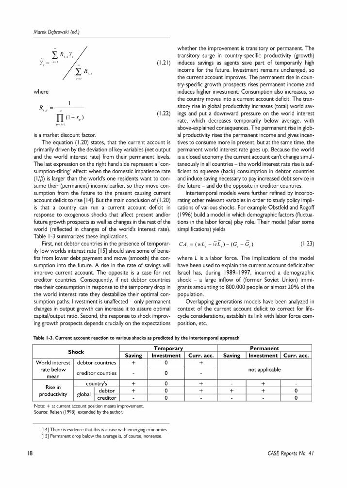
primarily driven by the deviation of key variables (net outputand the world interest rate) from their permanent levels.The last expression on the right hand side represent a "con-sumption-tilting" effect: when the domestic impatience rate(1/β) is larger than the world's one residents want to con-sume their (permanent) income earlier, so they move con-sumption from the future to the present causing currentaccount deficit to rise [14]. But the main conclusion of (1.20)is that a country can run a current account deficit inresponse to exogenous shocks that affect present and/orfuture growth prospects as well as changes in the rest of theworld (reflected in changes of the world's interest rate).Table 1-3 summarizes these implications.
First, net debtor countries in the presence of temporar-ily low worlds interest rate [15] should save some of bene-fits from lower debt payment and move (smooth) the con-sumption into the future. A rise in the rate of savings willimprove current account. The opposite is a case for netcreditor countries. Consequently, if net debtor countriesrise their consumption in response to the temporary drop inthe world interest rate they destabilize their optimal con-sumption paths. Investment is unaffected – only permanentchanges in output growth can increase it to assure optimalcapital/output ratio. Second, the response to shock improv-ing growth prospects depends crucially on the expectations
whether the improvement is transitory or permanent. Thetransitory surge in country-specific productivity (growth)induces savings as agents save part of temporarily highincome for the future. Investment remains unchanged, sothe current account improves. The permanent rise in coun-try-specific growth prospects rises permanent income andinduces higher investment. Consumption also increases, sothe country moves into a current account deficit. The tran-sitory rise in global productivity increases (total) world sav-ings and put a downward pressure on the world interestrate, which decreases temporarily below average, withabove-explained consequences. The permanent rise in glob-al productivity rises the permanent income and gives incen-tives to consume more in present, but at the same time, thepermanent world interest rate goes up. Because the worldis a closed economy the current account can't change simul-taneously in all countries – the world interest rate rise is suf-ficient to squeeze (back) consumption in debtor countriesand induce saving necessary to pay increased debt service inthe future – and do the opposite in creditor countries.
Intertemporal models were further refined by incorpo-rating other relevant variables in order to study policy impli-cations of various shocks. For example Obstfeld and Rogoff(1996) build a model in which demographic factors (fluctua-tions in the labor force) play role. Their model (after somesimplifications) yields
(1.23)
where L is a labor force. The implications of the modelhave been used to explain the current account deficit afterIsrael has, during 1989–1997, incurred a demographicshock – a large inflow of (former Soviet Union) immi-grants amounting to 800.000 people or almost 20% of thepopulation.
Overlapping generations models have been analyzed incontext of the current account deficit to correct for life-cycle considerations, establish its link with labor force com-position, etc.
∑
∑∞
=
∞
==
tsst
tssst
t
R
YRY
,
,~
∏+=
+
= s
tuu
st
rR
1
,
)1(
1
Table 1-3. Current account reaction to various shocks as predicted by the intertemporal approach
Temporary PermanentShock
Saving Investment Curr. acc. Saving Investment Curr. acc.debtor countries + 0 +World interest
rate belowmean creditor counties - 0 -
not applicable
country's + 0 + - + -debtor + 0 + + + 0
Rise inproductivity global
creditor - 0 - - - 0Note: + at current account position means improvement.Source: Reisen (1998), extended by the author.
[14] There is evidence that this is a case with emerging economies.[15] Permanent drop below the average is, of course, nonsense.
)~
()~~( ttttt GGLwwLCA −−−=
19
Currency Crises in Emerging Markets – Selected Comparative ...
CASE Reports No. 41
In spite of being theoretically well justified the intertem-poral models produce, under plausible parameter values,bizarre and unacceptable results. Numerical simulationsshow that the optimal reaction to external shocks is to runvery high current account deficits. After accumulating a verylarge external debt and as the shock dies out the economyswitches to equally implausible surpluses. Obstfeld andRogoff (1996) demonstrate, that a small open economy withconstant return to scale production function, domestic pro-ductivity growth exceeding that of the world, constantworld interest rate and no borrowing constraints should runa steady state surplus of about 50% of GDP. Similar modeldeveloped to understand the impact of financial liberaliza-tion for the external position and adapted to the case ofSpain show that after a financial reform Spain should haverun a deficit peaking at 60% of GDP. Analysis of the eco-nomic behavior of a small economy with investment instal-lation costs implies that Brazil should have accumulated aforeign debt of more than 300% of its GDP.
Such current account and debt/GDP ratios are notrecorded in reality and prove that relaying on the notion offrictionless economy (principally perfect capital mobility andno credit constraints) is of little help in explaining the actualevolution of current account behavior. Other variables thatmatter, sometimes hardly measurable, as the country's will-ingness to pay and foreigner's willingness to lend, should beincluded in the model.
Credit constraint received, particularly after the Mexi-can crises, special attention,. Their main assumption is thatthe authorities cannot borrow as much as they want on theworld market. When this constraint is introduced, themodel's behavior improves significantly. It also produces asituation in which a change in the level of the borrowingconstrain (a switch in market sentiment for example) canresult in a currency crisis.
There is an ongoing research on the links between bud-get and current account deficits or, in other words, whetherthe Lawson Doctrine is valid (and to what extent and whynot). First, if Ricardian equivalence holds budget deficitshould not matter at all [16] and the current account bal-ance is always an outcome of private sector decisions – sopeople who believe in Lawson Doctrine prove that theirdon't believe in Ricardian equivalence. On the other hand,the government behavior is distortionary and in practicethere is ample evidence that Ricardian equivalence doesn'thold – the estimated so-called Ricardian offset coefficientaverage around 0.5, which means, that 1% (of GDP)increase in government deficit raises the current accountdeficit by 0.5% (of GDP). There are more reasons why
Lawson Doctrine shouldn't hold. It can be argued that muchof the private sector debt is actually contingent public liabil-ity – governments have proven many times that when thingsgo wrong they step in and bail it out. Various deposit insur-ances are other kinds of the same thing. Moreover privatesector may hold excessively optimistic expectations aboutits permanent income level, financial market bubbles mayadd to the problem by discouraging private savings throughwealth effect.
1.3.3. How to Calculate a Sustainable CurrentAccount Deficit
Generally speaking there are two ways of calculating thesustainable current account. The first one bases on countryspecific knowledge and involves less quantitative but morenarrative (or rather intuitive) methods. The second one ismodel-based and requires the use (sometimes quite sophis-ticated) econometric tools and estimations.
1.3.3.1. Underlying Current Account BalanceThe former approach is usually implemented in the fol-
lowing way (known as "underlying current account bal-ance"). First step is to estimate (or rather project) how thecurrent account would develop in the near future if no newshocks arrive, i.e. at prevailing exchange rate, when thecountry and its neighbors operate at usual level of capacityutilization and when lagged effects of past shocks (changesin policies, in the terms of trade, in prices and other tem-porary factors) die out. This procedure yields an "underly-ing" current account balance. Second step involves deter-mining the sustainable (or "normal") level of savings-invest-ment gap consistent with a long-run equilibrium when thehome country and all its financial partners operate with lowinflation and without financial sector disturbances – this pro-cedure yields "normal" capital flows balance. In the thirdstep the two outcomes are compared and if they are farapart it means, that the current account position is unsus-tainable in the long run. This calculation requires relativelymuch country specific knowledge – its export structure,policy stance, past events and other factors should beknown and used in the procedure.
1.3.3.2. Model-based CalculationsThe second approach is usually done in the framework
of the theoretical model of the current account. For exam-ple, one can exploit the result that the current account(deficit) is equal to the present value of expected declines in
[16] So-called Ricardian equivalence is an outcome of an analysis in a forward-looking rational expectations framework and states that (under someassumptions) the way in which government finances itself does not matter for private sector decisions (consumption path). In this context it implies thatin the presence of increased budget spendings financed by bond issues private sector adjust immediately by increase in savings in expectations for futureincrease in taxes (to buy the debt back).
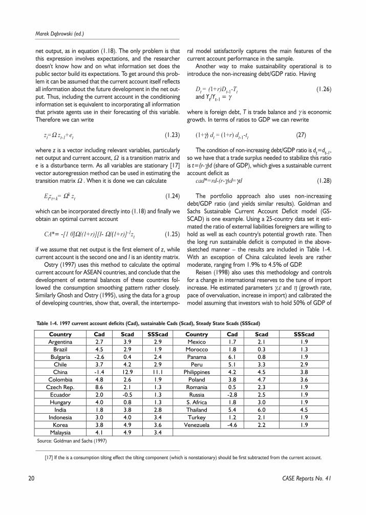
20
Marek D¹browski (ed.)
net output, as in equation (1.18). The only problem is thatthis expression involves expectations, and the researcherdoesn't know how and on what information set does thepublic sector build its expectations. To get around this prob-lem it can be assumed that the current account itself reflectsall information about the future development in the net out-put. Thus, including the current account in the conditioninginformation set is equivalent to incorporating all informationthat private agents use in their forecasting of this variable.Therefore we can write
zt=Ω zt-1+et (1.23)
where z is a vector including relevant variables, particularlynet output and current account, Ω is a transition matrix ande is a disturbance term. As all variables are stationary [17]vector autoregression method can be used in estimating thetransition matrix Ω . When it is done we can calculate
Etzt+k= Ωk zt (1.24)
which can be incorporated directly into (1.18) and finally weobtain an optimal current account
CA*= -[1 0]Ω/(1+r)][I- Ω/(1+r)]-1zt (1.25)
if we assume that net output is the first element of z, whilecurrent account is the second one and I is an identity matrix.
Ostry (1997) uses this method to calculate the optimalcurrent account for ASEAN countries, and conclude that thedevelopment of external balances of these countries fol-lowed the consumption smoothing pattern rather closely.Similarly Ghosh and Ostry (1995), using the data for a groupof developing countries, show that, overall, the intertempo-
ral model satisfactorily captures the main features of thecurrent account performance in the sample.
Another way to make sustainability operational is tointroduce the non-increasing debt/GDP ratio. Having
Dt = (1+r)Dt-1-Tt (1.26)and Yt/Yt-1 = γ
where is foreign debt, T is trade balance and γ is economicgrowth. In terms of ratios to GDP we can rewrite
(1+γ) dt = (1+r) dt-1-tt (27)
The condition of non-increasing debt/GDP ratio is dt=dt-1,so we have that a trade surplus needed to stabilize this ratiois t=(r-γ)d (share of GDP), which gives a sustainable currentaccount deficit as
cad*=rd-(r-γ)d=γd (1.28)
The portfolio approach also uses non-increasingdebt/GDP ratio (and yields similar results). Goldman andSachs Sustainable Current Account Deficit model (GS-SCAD) is one example. Using a 25-country data set it esti-mated the ratio of external liabilities foreigners are willing tohold as well as each country's potential growth rate. Thenthe long run sustainable deficit is computed in the above-sketched manner – the results are included in Table 1-4.With an exception of China calculated levels are rathermoderate, ranging from 1.9% to 4.5% of GDP.
Reisen (1998) also uses this methodology and controlsfor a change in international reserves to the tune of importincrease. He estimated parameters γ,ε and η (growth rate,pace of overvaluation, increase in import) and calibrated themodel assuming that investors wish to hold 50% of GDP of
CASE Reports No. 41
[17] If the is a consumption tilting effect the tilting component (which is nonstationary) should be first subtracted from the current account.
Table 1-4. 1997 current account deficits (Cad), sustainable Cads (Scad), Steady State Scads (SSScad)
Country Cad Scad SSScad Country Cad Scad SSScadArgentina 2.7 3.9 2.9 Mexico 1.7 2.1 1.9
Brazil 4.5 2.9 1.9 Morocco 1.8 0.3 1.3Bulgaria -2.6 0.4 2.4 Panama 6.1 0.8 1.9
Chile 3.7 4.2 2.9 Peru 5.1 3.3 2.9China -1.4 12.9 11.1 Philippines 4.2 4.5 3.8
Colombia 4.8 2.6 1.9 Poland 3.8 4.7 3.6Czech Rep. 8.6 2.1 1.3 Romania 0.5 2.3 1.9
Ecuador 2.0 -0.5 1.3 Russia -2.8 2.5 1.9Hungary 4.0 0.8 1.3 S. Africa 1.8 3.0 1.9
India 1.8 3.8 2.8 Thailand 5.4 6.0 4.5Indonesia 3.0 4.0 3.4 Turkey 1.2 2.1 1.9
Korea 3.8 4.9 3.6 Venezuela -4.6 2.2 1.9Malaysia 4.1 4.9 3.4
Source: Goldman and Sachs (1997)
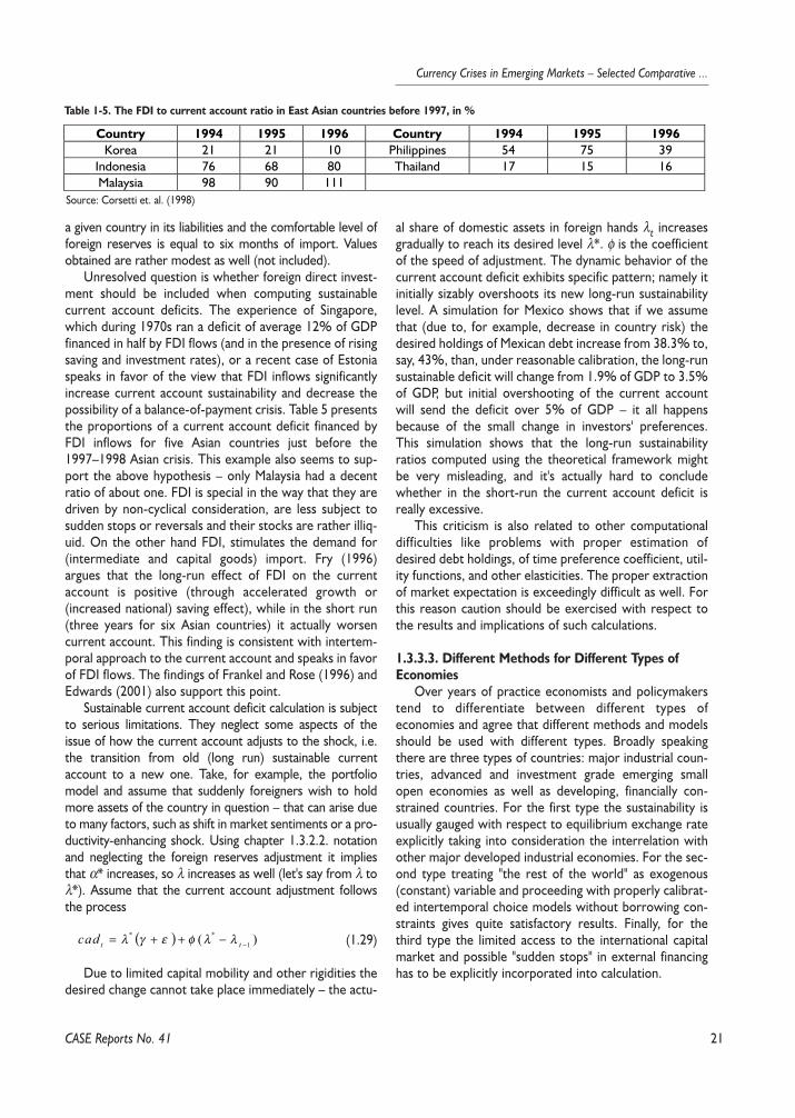
21
Currency Crises in Emerging Markets – Selected Comparative ...
CASE Reports No. 41
a given country in its liabilities and the comfortable level offoreign reserves is equal to six months of import. Valuesobtained are rather modest as well (not included).
Unresolved question is whether foreign direct invest-ment should be included when computing sustainablecurrent account deficits. The experience of Singapore,which during 1970s ran a deficit of average 12% of GDPfinanced in half by FDI flows (and in the presence of risingsaving and investment rates), or a recent case of Estoniaspeaks in favor of the view that FDI inflows significantlyincrease current account sustainability and decrease thepossibility of a balance-of-payment crisis. Table 5 presentsthe proportions of a current account deficit financed byFDI inflows for five Asian countries just before the1997–1998 Asian crisis. This example also seems to sup-port the above hypothesis – only Malaysia had a decentratio of about one. FDI is special in the way that they aredriven by non-cyclical consideration, are less subject tosudden stops or reversals and their stocks are rather illiq-uid. On the other hand FDI, stimulates the demand for(intermediate and capital goods) import. Fry (1996)argues that the long-run effect of FDI on the currentaccount is positive (through accelerated growth or(increased national) saving effect), while in the short run(three years for six Asian countries) it actually worsencurrent account. This finding is consistent with intertem-poral approach to the current account and speaks in favorof FDI flows. The findings of Frankel and Rose (1996) andEdwards (2001) also support this point.
Sustainable current account deficit calculation is subjectto serious limitations. They neglect some aspects of theissue of how the current account adjusts to the shock, i.e.the transition from old (long run) sustainable currentaccount to a new one. Take, for example, the portfoliomodel and assume that suddenly foreigners wish to holdmore assets of the country in question – that can arise dueto many factors, such as shift in market sentiments or a pro-ductivity-enhancing shock. Using chapter 1.3.2.2. notationand neglecting the foreign reserves adjustment it impliesthat α* increases, so λ increases as well (let's say from λ toλ*). Assume that the current account adjustment followsthe process
(1.29)
Due to limited capital mobility and other rigidities thedesired change cannot take place immediately – the actu-
al share of domestic assets in foreign hands λt increasesgradually to reach its desired level λ*. φ is the coefficientof the speed of adjustment. The dynamic behavior of thecurrent account deficit exhibits specific pattern; namely itinitially sizably overshoots its new long-run sustainabilitylevel. A simulation for Mexico shows that if we assumethat (due to, for example, decrease in country risk) thedesired holdings of Mexican debt increase from 38.3% to,say, 43%, than, under reasonable calibration, the long-runsustainable deficit will change from 1.9% of GDP to 3.5%of GDP, but initial overshooting of the current accountwill send the deficit over 5% of GDP – it all happensbecause of the small change in investors' preferences.This simulation shows that the long-run sustainabilityratios computed using the theoretical framework mightbe very misleading, and it's actually hard to concludewhether in the short-run the current account deficit isreally excessive.
This criticism is also related to other computationaldifficulties like problems with proper estimation ofdesired debt holdings, of time preference coefficient, util-ity functions, and other elasticities. The proper extractionof market expectation is exceedingly difficult as well. Forthis reason caution should be exercised with respect tothe results and implications of such calculations.
1.3.3.3. Different Methods for Different Types ofEconomies
Over years of practice economists and policymakerstend to differentiate between different types ofeconomies and agree that different methods and modelsshould be used with different types. Broadly speakingthere are three types of countries: major industrial coun-tries, advanced and investment grade emerging smallopen economies as well as developing, financially con-strained countries. For the first type the sustainability isusually gauged with respect to equilibrium exchange rateexplicitly taking into consideration the interrelation withother major developed industrial economies. For the sec-ond type treating "the rest of the world" as exogenous(constant) variable and proceeding with properly calibrat-ed intertemporal choice models without borrowing con-straints gives quite satisfactory results. Finally, for thethird type the limited access to the international capitalmarket and possible "sudden stops" in external financinghas to be explicitly incorporated into calculation.
Table 1-5. The FDI to current account ratio in East Asian countries before 1997, in %
Country 1994 1995 1996 Country 1994 1995 1996Korea 21 21 10 Philippines 54 75 39
Indonesia 76 68 80 Thailand 17 15 16Malaysia 98 90 111
Source: Corsetti et. al. (1998)
( ) )( 1**
−−++= ttcad λλφεγλ
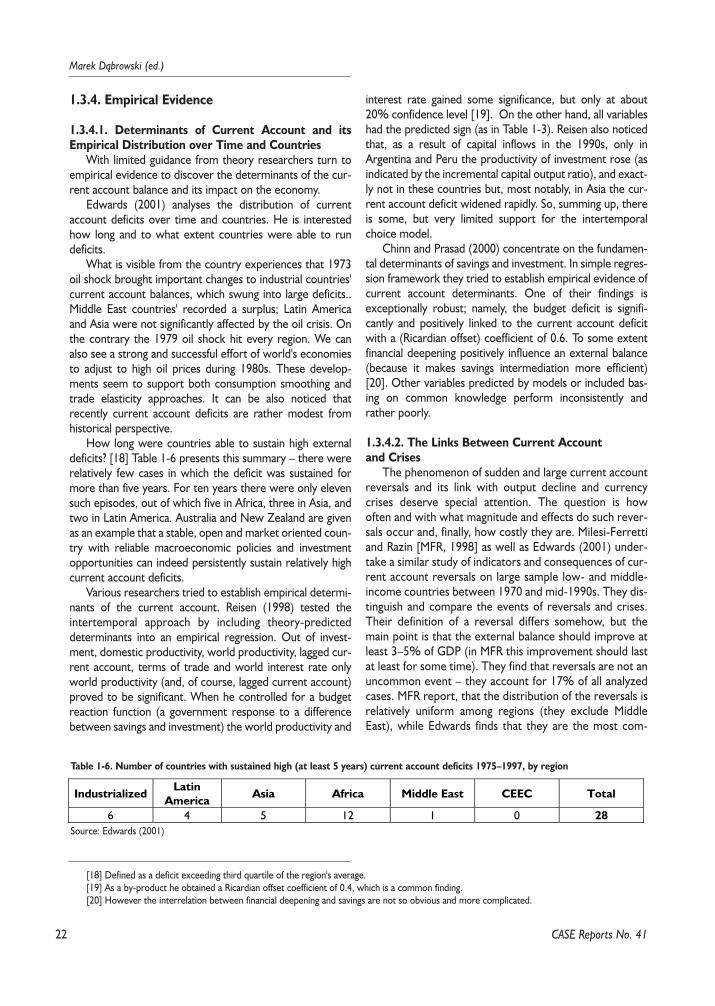
22
Marek D¹browski (ed.)
1.3.4. Empirical Evidence
1.3.4.1. Determinants of Current Account and itsEmpirical Distribution over Time and Countries
With limited guidance from theory researchers turn toempirical evidence to discover the determinants of the cur-rent account balance and its impact on the economy.
Edwards (2001) analyses the distribution of currentaccount deficits over time and countries. He is interestedhow long and to what extent countries were able to rundeficits.
What is visible from the country experiences that 1973oil shock brought important changes to industrial countries'current account balances, which swung into large deficits..Middle East countries' recorded a surplus; Latin Americaand Asia were not significantly affected by the oil crisis. Onthe contrary the 1979 oil shock hit every region. We canalso see a strong and successful effort of world's economiesto adjust to high oil prices during 1980s. These develop-ments seem to support both consumption smoothing andtrade elasticity approaches. It can be also noticed thatrecently current account deficits are rather modest fromhistorical perspective.
How long were countries able to sustain high externaldeficits? [18] Table 1-6 presents this summary – there wererelatively few cases in which the deficit was sustained formore than five years. For ten years there were only elevensuch episodes, out of which five in Africa, three in Asia, andtwo in Latin America. Australia and New Zealand are givenas an example that a stable, open and market oriented coun-try with reliable macroeconomic policies and investmentopportunities can indeed persistently sustain relatively highcurrent account deficits.
Various researchers tried to establish empirical determi-nants of the current account. Reisen (1998) tested theintertemporal approach by including theory-predicteddeterminants into an empirical regression. Out of invest-ment, domestic productivity, world productivity, lagged cur-rent account, terms of trade and world interest rate onlyworld productivity (and, of course, lagged current account)proved to be significant. When he controlled for a budgetreaction function (a government response to a differencebetween savings and investment) the world productivity and
interest rate gained some significance, but only at about20% confidence level [19]. On the other hand, all variableshad the predicted sign (as in Table 1-3). Reisen also noticedthat, as a result of capital inflows in the 1990s, only inArgentina and Peru the productivity of investment rose (asindicated by the incremental capital output ratio), and exact-ly not in these countries but, most notably, in Asia the cur-rent account deficit widened rapidly. So, summing up, thereis some, but very limited support for the intertemporalchoice model.
Chinn and Prasad (2000) concentrate on the fundamen-tal determinants of savings and investment. In simple regres-sion framework they tried to establish empirical evidence ofcurrent account determinants. One of their findings isexceptionally robust; namely, the budget deficit is signifi-cantly and positively linked to the current account deficitwith a (Ricardian offset) coefficient of 0.6. To some extentfinancial deepening positively influence an external balance(because it makes savings intermediation more efficient)[20]. Other variables predicted by models or included bas-ing on common knowledge perform inconsistently andrather poorly.
1.3.4.2. The Links Between Current Accountand Crises
The phenomenon of sudden and large current accountreversals and its link with output decline and currencycrises deserve special attention. The question is howoften and with what magnitude and effects do such rever-sals occur and, finally, how costly they are. Milesi-Ferrettiand Razin [MFR, 1998] as well as Edwards (2001) under-take a similar study of indicators and consequences of cur-rent account reversals on large sample low- and middle-income countries between 1970 and mid-1990s. They dis-tinguish and compare the events of reversals and crises.Their definition of a reversal differs somehow, but themain point is that the external balance should improve atleast 3–5% of GDP (in MFR this improvement should lastat least for some time). They find that reversals are not anuncommon event – they account for 17% of all analyzedcases. MFR report, that the distribution of the reversals isrelatively uniform among regions (they exclude MiddleEast), while Edwards finds that they are the most com-
CASE Reports No. 41
Table 1-6. Number of countries with sustained high (at least 5 years) current account deficits 1975–1997, by region
IndustrializedLatin
AmericaAsia Africa Middle East CEEC Total
6 4 5 12 1 0 28Source: Edwards (2001)
[18] Defined as a deficit exceeding third quartile of the region's average.[19] As a by-product he obtained a Ricardian offset coefficient of 0.4, which is a common finding.[20] However the interrelation between financial deepening and savings are not so obvious and more complicated.
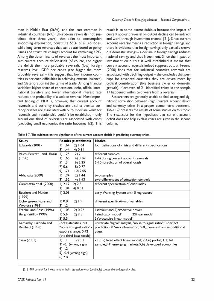
23
Currency Crises in Emerging Markets – Selected Comparative ...
mon in Middle East (26%), and the least common inindustrial countries (6%). Short-term reversals (not sus-tained after three years), that point to consumptionsmoothing explanation, constitute 55% of all episodes,while long-term reversals that can be attributed to policyissues and structural changes account for remaining 45%.Among the determinants of reversals the most importantare: current account deficit itself (of course, the biggerthe deficit the more probable reversal), (low) foreignreserves level, GDP per capita (the bigger the moreprobable reversal – this suggest that low income coun-tries experience difficulties in achieving external balance)and (deterioration in) the terms of trade. Among financialvariables: higher share of concessional debt, official inter-national transfers and lower international interest ratereduced the probability of a sudden reversal. Most impor-tant finding of MFR is, however, that current accountreversals and currency crashes are distinct events: cur-rency crashes are associated with output decline while forreversals such relationship couldn't be established – onlyaround one third of reversals are associated with crises(excluding small economies the ratio becomes 1/2). This
result is to some extent dubious because the impact ofcurrent account reversal on output decline can be indirectand work through investment channel [21]. Since currentaccount reversal means a reduction in foreign savings andthere is evidence that foreign savings only partially crowdout domestic savings – a decline in foreign savings reducesnational savings and thus investment. Since the impact ofinvestment on output is well established it means thatcurrent account reversals indeed suppress output. Freund(2000) finds that for industrial countries reversals areassociated with declining output – she concludes that per-haps for advanced countries they are driven more bycyclical consideration (like business cycles or domesticgrowth). Moreover, of 21 identified crises in the sample17 happened within two years from a reversal.
Researchers are generally unable to find strong and sig-nificant correlation between (high) current account deficitand currency crises in a proper econometric treatment.Table 1-7 presents the results of some studies on this topic.The t-statistics for the hypothesis that current accountdeficit does not help explain crises are given in the secondcolumn.
CASE Reports No. 41
Table 1-7. The evidence on the significance of the current account deficit in predicting currency crises
Study Results (t-statistics) NoticeEdwards (2001) 1) 1.64 2) 1.64
3) 1.44 4) 0.31four definitions of crisis and different specifications
Milesi-Ferretti and Razin(1998)
1) 1.25 2) 23) 1.65 4) 0.365) 1.3 6) 2,257) 0.6 8) 0.779) 1.71 10) 2.05
different samples1-4) during current account reversals5-10) prediction of overall crash
Abhuvalia (2000) 1) 1.94 2) 1.443) 1.52 4) 1.43
two samplestwo different set of contagion controls
Caramazza et.al. (2000) 1) 2.17 2) 2.53) 1.84 4) 0.51
different specification of crisis index
Bussiere and Mulder(1999)
1) 2.03 early Warning System with 5 regressors
Eichengreen, Rose andWyplosz (1996)
1) 0.8 2) 1.93) 1.2
different specification of variables
Frankel and Rose (1996) 1) 1.03 2) 0.22 1)default and 2)predictive powerBerg Pattillo (1999) 1) 5.6 2) 9.5
3) 5.51)'indicator model' 2)linear model3)"piecewise linear model"
Kaminsky, Lizondo andReinhart (1998)
-not t-statistics, but“noise to signal ratio” -export change: 0.42(the third best result)
univariate "signal" analysis, "noise to signal ratio"; 0-perfectprediction, 0.5-no information, >0,5 worse than unconditionalguess
Sasin (2001) 1) 1.1 2) 3.13) -0.1(wrong sign)4) 1.25) -0.4 (wrong sign)6) 2.8
- 1,3,5) fixed effect linear model; 2,4,6) probit; 1,2) fullsample;3,4) emerging markets;5,6) developed economies
[21] MFR control for investment in their regression what (probably) causes the endogeneity bias.
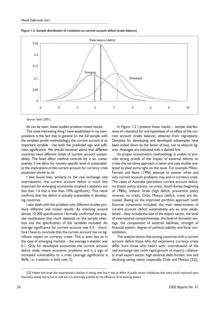
24
Marek D¹browski (ed.)
As can be seen, these studies produce mixed results.The most interesting thing I have established in my com-
putations is the fact that in general (in the full sample withthe simplest probit methodology) the current account is animportant variable – has both the predicted sign and suffi-cient significance. We should however admit that differentcountries have different levels of current account sustain-ability. The fixed effect method controls for it so, conse-quently, if we allow for country-specific level of sustainabili-ty the implications of the current account for currency crisisprediction shrink to nil.
I also found that, similarly to the real exchange rateovervaluation, the current account deficit is much lessimportant for emerging economies (implied t-statistics areless than 1.6 that is less than 10% significant). This resultconfirms that the deficit is actually sustainable in develop-ing countries
I also dealt with the problem why different studies pro-duce different and mixed results. By checking aroundalmost 10,000 specifications I formally confirmed the pop-ular explanation that much depends on the sample selec-tion and the specification of the variables included. Anaverage significance for current account was 0.5 – there-fore I have to conclude that the current account has no sig-nificant impact on currency crises. This is even less so inthe case of emerging markets – the average t-statistic was0.1. Only for developed economies the current accountdeficit really means economic problems and is a sign ofincreased vulnerability to a crisis (average significance is96%, i.e. t-statistic is little over 2).
In Figure 1-2 I present these results – sample distribu-tions of t-statistics for null hypothesis of no effect of the cur-rent account (trade balance) obtained from regressions.Densities for developing and developed subsamples havebeen scaled down by the factor of two, not to obscure fig-ures. Averages are indicated with a dashed line.
As proper econometric methodology is unable to pro-vide strong proofs of the impact of external deficits oncrises the narrative approach is taken and case studies ana-lyzed to shed some light on the issue. For example Milesi-Ferretti and Razin (1996) attempt to answer when andwhy current account problems may end in currency crisis.The cases of Australia (persistent current account deficit,no drastic policy actions, no crisis), South Korea (beginningof 1980s), Ireland, Israel (high deficit, preventive policyreversal, no crisis), Chile, Mexico (deficit, crisis) are dis-cussed. Basing on the improved portfolio approach (withfinancial constraints included) the main determinants ofcurrent account deficit sustainability are ex ante estab-lished – they include the size of the export sector, the levelof international competitiveness, the level of domestic sav-ings, the composition of external liabilities, strength offinancial system, degree of political stability and fiscal con-solidation.
The analysis shows that among countries with a currentaccount deficit those who did experience currency crisesdiffer from those who hadn't with: overvaluation of thereal exchange rate (with rapid growth of import), relative-ly small export sector, high external debt burden, low anddeclining saving ration (especially Chile and Mexico [22]),
CASE Reports No. 41
Figure 1-2. Sample distribution of t-statistics on current account deficit (trade balance)
0.25
0.2
0.15
0.1
0.05
0
-6 -4 -2 0 2 4 6 8 10
Trade balance (deficit)
Developed
Emarging
Source: Sasin (2001).
[22] Ireland and Israel also experienced a decline in saving rates but it was an effect of public sector imbalances that were much improved upon.Australia's saving rate is low as well but it is seemingly justified by the efficiency of its banking system.
25
Currency Crises in Emerging Markets – Selected Comparative ...
political instability (elections in Mexico) and the composi-tion of capital inflows [23]. All countries arranged devalu-ation, but some were preventive and successful (Australia,Israel), while some countries were forced to do it by thecrises (Chile, Mexico).
1.4. Conclusions
We tried to establish the links between real exchange rateovervaluation, current account deficit and currency crises.The evidence is that real exchange rate helps explain and pre-dict crisis. To some extent this result is intuitive or even tau-tological. On the other hand, the results on the currentaccount deficit are mixed – proper econometric methodolo-gy fails to find strong support that the current account deficitactually is and underlying cause of a crisis. But qualitativeanalysis and common knowledge views large current accountdeficits as dangerous. The notion of "new crisis" gives thedeficit secondary, but important role. Although financial vari-ables, such as the level of short term debt, the state of thebanking sector, moral hazard, balance sheet problems aremain causes of sudden capital outflow, which in turn ignitescrisis and damages economy – the current account is the sig-nal that the domestic policies can be unsustainable and for-eign reserves (a must for foreign debt repayment) could besoon depleted. Recently, it is also not so important if theexternal deficit is driven by public or private imbalances –rather source of the deficit and its financing matters.
Because of the above-mentioned reasons currentaccount is still and important variable, on which investorsbase their decisions. We have, however established that theactual size of the current account cannot be the only basisof current account sustainability judgement. What is todaysustainable can other time become unsustainable, wheninternational capital markets sentiment changes.
It all can be well summarized using the words of Ostry(1997), who yet before the Asian crisis warned thatalthough Asian current account deficits safely match theconsumption smoothing pattern other factors may affectexternal sustainability. He highlighted the role of the leveland composition of external liabilities, the flexibility ofmacroeconomic policies, the efficiency of investment, thestate of the financial system. He concluded that even if theexternal position seems sustainable in views of all majormodels and determinants there is a case to reduce currentaccounts deficits in order to minimize the risk that arisefrom running these deficits in the presence of the above-mentioned weaknesses.
CASE Reports No. 41
[23] Australia relied more on equity (significant part of the debt were also denominated in domestic currency, it had a developed bond market). Insuch case risk shared by foreigner investor. Ireland, in turn, had a large and sustainable inflow of FDI's.
26
Marek D¹browski (ed.)
References
Ades A., F. Kaune (1997). "A New Measure of CurrentAccount Sustainability for Developing Countries". Goldman-Sachs Emerging Markets Economic Research.
Ahluwalia P. (2000). "Discriminating Contagion: an Alter-native Explanation of Contagious Currency Crises in Emerg-ing Markets, IMF/WP/00/14
Aziz J., F. Caramazza, R. Salgado (2000). "CurrencyCrises: in Search of Common Elements". IMF/WP/00/67.
Baig T., I. Goldfajn (1998). "Financial Market Contagionin the Asian Crisis". IMW/WP/98/155.
Berg A., C. Pattillo (1999). "Predicting Currency Crises:the Indicator Approach and an Alternative". Journal of Inter-national Money and Finance, 18, 561–586.
Bussiere M., C. Mulder (1999). "External Vulnerability inEmerging Market Economies: How High Liquidity Can Off-set Weak Fundamentals and the Effects of Contagion.IMF/WP/99/88.
Calvo G.A., L. Leiderman, C. Reinhart (1993). "CapitalInflows and Real Exchange Rate Appreciation in Latin Amer-ica: the Role of External Factors." IMF/SP/40.
Calvo G., E. Mendoza (1998). "Empirical Puzzles ofChilean Stabilization Policy". Duke University.
Caramazza F., L. Ricci, R. Salgado (2000). "Trade andFinancial Contagion in Currency Crises". IMF/WP/00/55.
Chinn M.D. (1998). "Before the Fall: Were East AsianCurrencies Overvalued?". NBER.
Chin M.D., E.S. Prasad (2000). "Medium-term Determi-nants of Current Accounts in Industrialized Countries: anEmpirical Exploration". NBER 7581.
Clark P.B., R. MacDonald (1998). "Exchange Rates andEconomic Fundamentals: a Methodological Comparison ofBEERs and FEERs". IMF/WP/98/67.
Cooper R.N. (1971). "Currency Devaluation in Develop-ing Countries". Essays in International Finance, 86, PrincetonUniversity.
Corsetti G., P. Pesenti, N. Roubini (1998). "What Causedthe Asian Currency Crisis". Banca d'Italia.
Dabos M., H.V. Juan-Ramos (2000). "Real Exchange RateResponse to Capital Flows in Mexico: an Empirical Analysis."IMF/WP/00/108.
Dornbusch R. (1998). "Asian Crisis Themes". MIT.Dornbusch R. (2001). "A Primer on Emerging Market
Crises". MIT.Dornbusch R., I. Goldfajn, R.O. Valdes (1995). "Curren-
cy Crises and Collapses". Brookings Papers on EconomicActivity, 1, 219–270.
Edwards S. (1998). "Capital Flows, Real Exchange Rates,and Capital Controls: some Latin American Experiences".NBER 6800.
Edwards S. (2000). "Exchange Rate Regimes, CapitalFlows and Crisis Prevention". NBER.
Edwards S. (2001). Does the Current Account Matter?".Paper presented on the conference on crises prevention inFlorida, January 2001.
Eichengreen B., A. Rose, Ch. Wyplosz (1996). "Conta-gious Currency Crises:. NBER 5681.
Forbes K.J. (2000). "How Important is Trade in the Inter-national Spread of Crises". Paper presented on the confer-ence on crises prevention in Florida, January 2001.
Frankel, Rose A. (1996). "Currency Crashes in EmergingMarkets". Journal of International Economics 41, 309.
Freund C.L. (2000). "Current Account Adjustment inIndustrialized Countries". FRB/IFDP 692.
Fry M. (1996). "How Foreign Direct Investment in Pacif-ic Asia Improves the Current Account". Journal of AsianEconomics, 7.
Gerlach S., F. Smets (1994). "Contagious SpeculativeAttacks". CEPR 1055.
Ghosh A.R., J.D. Ostry (1995). "The Current Account inDeveloping Countries: a Perspective from the ConsumptionSmoothing Approach". The World Bank Economic Review9, no. 2, 305–333.
Glick R., A. Rose (1999). "Contagion and Trade: Why AreCurrency Crises Regional". Journal of International Moneyand Finance, 18, 603–617.
Goldfajn I., R.O. Valdes (1996). "The Aftermath ofAppreciation". NBER 5650.
Goldfajn I., R.O. Valdes (1998). "Are Currency CrisesPredictable?". European Economic Review, 42, 874–885.
Goldman Sachs. Emerging Markets Economic Research.Kaminsky G., S. Lizondo, C. Reinhart (1998). "Leading
Indicators of Currency Crises". IMF.Knight M., F. Scacciavillani (1998). "Current Account:
What is Their Relevance for Economic Policy Making?".IMF/WP/98/71.
MacDonald R., M. Taylor (1994). "The Monetary Modelof the Exchange Rate: Long-run Relationship, Short-runDynamics and How to Beat a Random Walk". Journal ofInternational Money and Finance, 13, 276–290.
Mark N. (1995). "Exchange Rates and Fundamentals: Evi-dence on Long Horizon Predictability". American EconomicReview, 85, 276–218.
Masson P. (1998). "Contagion: Monsoonal Effects, Spilloversand Jumps between Multiple Equilibria". IMF/WP/98/142.
Meese R.A., K. Rogoff (1983). "Empirical Exchange RateModels of the Seventies: do They fit out of Sample?". Journalof International Economics, 14, 3–24.
Milesi-Ferretti G.M., A. Razin (1996). "Sustainability ofPersistent Current Account Deficits". NBER 5467.
Milesi-Ferretti G.M., A. Razin (1996b). "Current AccountSustainability: Selected East Asian and Latin American Expe-riences". NBER 5791.
Milesi-Ferretti G.M., A. Razin (1999). "Current AccountReversals and Currency Crises: Empirical Regularities".IMF/WP/98/89.
CASE Reports No. 41
27
Currency Crises in Emerging Markets – Selected Comparative ...
Obstfeld M., K. Rogoff (1996). "The Foundations ofInternational Macroeconomics". Cambridge, MIT Press.
Ostry J.D. (1997). "Current Account Imbalances inASEAN Countries: are They a Problem?". IMF/WP/97/51.
Reisen H. (1998). "Sustainable and Excessive CurrentAccount Deficits". OECD TP 132.
Sachs J. (1981). "The Current Account and the Macro-economic Adjustment in the 1970s". Brookings Papers onEconomic Activity, 201-268.
Sachs J., A. Tornell, A. Velasco (1995). "Lessons fromMexico". Harvard University.
Sachs J., A. Tornell, A. Velasco (1996). "Financial Crisesin Emerging Markets: the Lessons of 1995". BrookingPapers on Economic Activity, 1, 147–217.
Sachs (1997). Personal view, Harvard University.Sasin M. (2001). "Predicting Currency Crises: the Ulti-
mate Significance of Macroeconomic Fundamentals in Lin-ear Specifications with Nonlinear Extensions". CASE S&A224.
World Economic Outlook.
CASE Reports No. 41
29
Currency Crises in Emerging Markets – Selected Comparative ...
CASE Reports No. 41
2.1. Introduction
The paper addresses a set of issues regarding thechoice of an exchange rate regime in financially fragileemerging markets. It provides an insight of how differentregime choices were connected with currency crashesduring 1990s. Fourteen cases of financial crises are exam-ined, and the decisions about the regime choice are dis-cussed in the light of costs associated with ending anarrangement weighted against the costs of further supportof a peg.
The analysis starts from the general discussion of whatregime choice is better for a "small open and emerging "economy. Specific issues related to the policy choice whendomestic currency comes under pressure are discussednext. The issue of empirical measurement of the costs andbenefits associated with the regime change is discussedusing case studies. The countries under consideration aregrouped into these that followed a hard peg regime beforethe crises, these that followed more relaxed types of pegs,and these that allowed their currencies to fluctuate. Therelative flexibility of an exchange rate regime is assessedwith the use of an "effective exchange rate flexibilityindex". Last section tries to quantify the influence of dif-ferent factors on the duration of exchange rate peg usinglogit analysis.
In the light of the following discussion, it seems that inthe majority of cases, where authorities decided to abandona peg, the problem was not really associated with the choice
whether to abandon the fixed rate or to stay on. Furthersupport of the exchange rate was in most cases prohibitive-ly expensive, so there was no choice in this respect. Rather,the problems experienced by these economies and magni-fied by the currency crashes showed inconsistency of pur-sued policies within the chosen exchange rate regime.
2.2. Old Dilemma: Fixed or Flexible?
The classic principle of the fixed versus flexible ratesdebate is that of Robert Mundell (1960). Under a highdegree of capital mobility, fixed exchange rate may dominateflexible exchange rate, in the sense of better stabilising prop-erties in the face of exogenous shock. Mundell proposed afirst explicit analysis of macroeconomic dynamics underfixed and flexible exchange rates. The main logic was thatunder a fixed exchange rate the interest rate has a directeffect on the external market to which it responds [1],therefore helping to quickly restore equilibrium. Whileunder flexible exchange rate regime the rate of interest hasa more direct effect on the external market than on thegoods and services market, to which it responds, leading toa cyclical adjustment. However, Mundell also wrote aboutsome limitations of fixed rates. Specifically, he noted that it isimportant for the fixed exchange rate system to be backedby the sufficient amount of international reserves. Mundellalso pointed on the fact that speculative attacks may posesmaller threat for the flexible exchange rate systems.
Part II.Choice of Exchange Rate Regime and Currency Crashes –Evidence of Some Emerging EconomiesMa³gorzata Jakubiak
[1] The actual rate of interest remains near its equilibrium level, and the disequilibrium at the goods and services market is eliminated by the pricelevel changes that affect the balance of payments.
30
Marek D¹browski (ed.)
CASE Reports No. 41
Recent waves of currency crises brought about new lit-erature, which tries to assess what regime choice is betterwhen a currency comes under pressure. And in this lightfixed exchange rate arrangements are not automaticallysuperior to flexible ones, especially when we consider thecosts of ending a peg.
There are important consequences of a sudden devalua-tion, when a currency comes under pressure in an emergingmarket country following a peg. Mishkin (1999) underlinesthat it is typically for an emerging market country followinga peg to have a large amount of debt denominated in foreigncurrency, because of uncertainty towards domestic money.In this case, devaluation produces high increase of the debtburden. This, in turn, leads to a decrease of net worth, low-ers investment and slows down economic activity.
Mishkin (1999) explains that the debt often has lowmaturity, and when a monetary authority rises interest rateswhen trying to defend domestic currency, economic agentssee their interest payments increasing, which further deteri-orates their balance sheets, and brings a fall in lending. Nev-ertheless, the larger the debt stock, the more valuable thepeg becomes for the authorities, and the authorities aremore committed to defend it, unless it becomes prohibi-tively expensive.
Chang and Velasco (1999) explore the topic of an opti-mal level of international reserves under a fixed exchangerate system. They write that under a fixed exchange rateregime, the possibility of a crisis when a currency comesunder pressure depends only on the underlying liquidity ofthe economy. This is to say, that if a country does not holda sufficient amount of foreign currency – and it should beremembered that keeping large reserves is costly – and isfollowing a peg, then a currency crisis occurs if only publicrealise that the central bank cannot meet its liabilities.
Contrary to this, flexible exchange rates can be superiorto the fixed rates, but under certain conditions. Floatingrates, in the view of the authors, lead to the point, where itis not optimal for the investors to withdraw early domesticcurrency deposits. Even if a run on domestic currencydenominated securities starts it is not optimal to move early,since there is a perception that all the obligations will behonoured, and depreciation punishes early withdrawals.This result holds when the proportion of domestic curren-cy deposits is large in relation to the foreign currencydeposits. The flexible exchange rate regime should beaccompanied by the appropriate monetary policy, namelythe central bank acting as a lender of last resort. Authorsstress that the result holds for the floating exchange rateregimes and not in the case of a sudden regime change.
It is also argued that greater integration with the worldcapital markets reduces benefits form exchange rate stabili-ty, increasing the optimal flexibility of exchange rate regime[Aizenman, Hausmann, 2000]. However, emerging marketcountries are usually not the ones that are characterised by
the large access to the world financial markets. This issuewill not be explored later in details, but high degree of inte-gration with the world financial market was certainly not thecase of Latin American or the CIS countries considered inthis paper. If we take an example of Argentina, it turns outthat overall capital flows constituted only 5% of its GDPbefore the Tequila crisis.
2.3. Costs of a Sudden Shift to a MoreFlexible Arrangement
If we summarise some of the insights pointed out in theprevious section, we can specify certain important costs ofa sudden change in the exchange rate regime that are of par-ticular significance for an emerging economy. Here, theemphasis is put on the costs of quitting fixed exchange ratearrangement, which are especially relevant in the light of thecase studies described later. Particularly, the costs related tothe initial defence and then the abandonment of a peg areunderlined. It is irrelevant here whether a fixed commit-ment is a declared one, or an implicit, but a perfectly knownto the public.
First of all, the sudden regime change produces fluctua-tions of output and investment. These fluctuations are trans-mitted to the real sector through the changing magnitude ofreal interest rates. But the determination of the long-termcosts of quitting a peg is beyond the scope of this paper,since they depend also on the evolution of a number ofmacroeconomic fundamentals, specific for a given economy.It is almost impossible to look at these costs only from theperspective of the different behaviour of nominal exchangerate. The more detailed discussion on modelling thesedynamics can be found in Cespedes, Chang, and Velasco(2000), Chang and Velasco (1999) – model with banks asintermediates, or Pitt (2001).
Nevertheless, there are several issues that are immedi-ately valid while taking the decision whether to defend afixed rate or let the currency to adjust, especially within thecontext of emerging or "transitional" countries describedlater. These issues are listed below.
Loss of international reserves. Starting from theperiod when the currency comes under the pressure andthe authorities decide to support its value, they use theirinternational reserves in order to ease the pressure. As itwill be later shown in the discussion of case studies, whenthe perception of the currency overvaluation and theattack are strong enough, the loss of internationalreserves is immediate and substantial. It creates the liq-uidity cost for the authority, which may undermine credi-bility of the central bank, and hence add to the expecta-tion spiral. Sufficient reserves are necessary in order to
31
Currency Crises in Emerging Markets – Selected Comparative ...
CASE Reports No. 41
sustain a peg. And if they are used up, then there is a needto rebuild them later, which may require time and exter-nal borrowing.
The importance of keeping high enough level of foreignreserves is emphasised in the model of balance-of-paymentscrises of Mendoza and Uribe (1999). The currency crashesthere occur as the result of prevailing large real appreciationand trade deficits, eventually triggered by the stance of fiscalpolicy. But the core issue is that the probability of a collapseof an exchange peg depends on the sensitivity of speculativecapital outflows to changes in foreign reserves. The proba-bility of a crisis and a currency risk premium are thus adecreasing function of the existing stock of reserves.Authors write that the changes in foreign exchange reservesare formulated endogenously, by the rational choices of pri-vate agents. While the peg is in place, they are the result ofa government budget constraint regarding fiscal policy vari-ables and the decisions of private sector agents.
Higher price of debt servicing. A rise in debt servic-ing in terms of domestic currency is an important threat oflarge depreciation for heavily indebted countries. And, aswill be shown later on, emerging economies are usuallyhighly indebted. This higher debt burden substantially weak-ens fiscal positions. The level of indebtedness and the per-centage of foreign currency denominated debt are thus agood indicator of how valuable is stable domestic currency– or a declared peg – for a given country.
Pitt (2001) provides a model, in which the linkbetween institutions and costs and benefits of the fixedexchange rate runs through foreign indebtedness and pro-ductivity of investment. When the speculations on theexchange rate start, government trades off the costs ofdevaluation in terms of higher debt service for the slow-down of economic growth through interest rate increaseswhen defending a peg.
Collapse in the demand for money. Especially visi-ble as a rise in domestic currency substitution. This causesproblems in banking sector (or difficulties in the recoveryof the banking sector, as, for example, it happened in theKyrgyz Republic after the Russian crisis). The banking sec-tor in emerging or transforming markets is usually charac-terised by the high volume of non-performing loans.Adding to this a decline in confidence to domestic curren-cy, which demonstrates itself in the form of decreasingholdings of the treasury bonds and withdrawals ofdeposits, we have a serious threat to the stability of finan-cial intermediation. This also limits the effectiveness of amonetary policy, and may hamper the necessary develop-ment of domestic financial market.
Rise in a country risk premium. This factor weakensaccess to the international creditors and lowers probabilityof attracting long-term capital inflows. Even setting aside allthe externality-related benefits of long-term foreign capitalcoming to the growing emerging market, continuous inflows
of foreign funds allow to build exchange reserves and to ser-vice external debt, even in a presence of large CA deficits.And as it is described later on, the lack of capital inflows mayquickly lead to unstable macroeconomic situation for anemerging economy.
High interest rates. Elevated nominal interest ratestend to limit investment. They result from the previouslydiscussed time-varying country risk-premiums, and inducedistortionary effects also on saving. However, if a country isdependent on foreign financing, and its perceived risk ishigher, there seem to be no other choice than rise interestrates in order to acquire new external credit.
Lost credibility. Following a sudden change in theexchange rate regime, and the turbulence lasting for sometime after, policy of the monetary authority may be per-ceived as less credible. Economic agents may behave in linewith their own expectations, which do not need to fullyreflect the authorities' commitment. This affects negativelythe process of disinflation, and creates an obstacle for quickrecovery. A country may find itself in a situation where thedomestic currency cannot be used for a long-term borrow-ing, even domestic. Domestic investments face either a cur-rency mismatch (projects that generate domestic currencyrevenues are financed with dollars) or a maturity mismatch(long-term projects must be financed with short-term bor-rowing). Then a country is permanently in a fragile state,almost independently of a chosen exchange rate regime. If acountry follows a float, and a shock occurs, the currencymismatch may cause bankruptcies. But if the authorities aretrying to defend a peg thus rising interest rates, this will pre-cipitate defaults on the short-term debts. Eichengreen andHausmann (1999) propose that in such situation it is advis-able to allow for a full dollarisation.
This credibility loss can be measured by the decrease inthe maturity of the debt, both foreign and domestic. And, itis often the case, as in some transition countries examinedby Ganev et al. (2001), that the dynamics of credibility of theexchange rate policy are mirrored by the dynamics of dol-larisation ratios.
2.4. Why Emerging Markets Peg theirCurrencies
If we know that pegging a currency may become cost-ly for an emerging country, why do these countries peg?First of all, fixed regimes are often introduced in order to"borrow stability". Under the condition that governments'commitments are credible, pegged regimes promote pre-dictability, tend to reduce inflationary expectations by pro-viding a nominal anchor, and – by eliminating exchange raterisk – ease trade and investment relations. If the commit-

32
Marek D¹browski (ed.)
CASE Reports No. 41
ment to keep the rate fixed is perceived as credible, coun-try risk premium falls, facilitating access to world financialmarkets. Another argument in favour of a fixed rate maybe this of lower domestic interest rates. Moreover, theeconomies that opt for fixing the exchange rate oftenexperience a currency substitution. If such "dollarised"economies are prone to shocks of financial nature, thenopting for a fixed rate automatically reduces monetaryvolatility.
2.5. Choices Faced after a Currency Col-lapse
It is clear that the decision to continue support for thepeg by a monetary authority when high devaluation pres-sures are mounting depends on the underlying costs. Thefirst choice of whether to keep the commitment to a fixedrate and continue losing reserves (lowering own credibility,and maybe hurting weak domestic banking sector) isweighted against the choice of letting the currency to depre-ciate with all described consequences. Assuming that stick-ing to the peg becomes prohibitively expensive at somepoint and the central bank flows the currency, there comesthe next choice – what to do after. This issue is exploredlater with the use of the case studies, but some general con-siderations are marked here.
The monetary authority may opt for repegging. Thechoice may seem questionable at first, but it may be anoption in the medium-term, after the exchange rate willreach its equilibrium level after an initial overshooting. Thetransition period must be long enough for two reasons. If anew peg is set too quickly, the exchange rate may be toodepreciated and not consistent with the medium-term fun-damentals. Secondly, after running out of reserves duringthe currency crisis the monetary authority may have prob-lems with gaining enough credibility. From the countries dis-cussed below, it was Malaysia who repeg its currencyapproximately one year after the crisis.
Repegging may not be an option also for the reason thatin many transition countries stabilisation policies have a badrecord. And it is difficult for the conventional fixed regimeto be credible. Then there may be two ways out: adoptinga currency board or even allowing for a full dollarisation, orlet the exchange rate to float. The main argument in favourof the first choice is that in some cases it may not be too badto give up an independent monetary policy. The fully float-ing exchange rate may also have some advantages, especial-
ly when the level of international reserves is low, providedthat there is enough transparency and the anchor for themonetary policy is set in an explicit way.
2.6. Empirical Evidence – Case Studies
This section describes further the issues of costs andadvantages of sudden devaluation under a fixed rateregime by the use of several case studies. The majority ofreviewed countries are the ones that followed a peg priorto the crisis, and then devalued. There are also threeexamples of economies that were allowing their curren-cies to fluctuate before the crises. These are contrastedwith one example of an economy that followed theextreme version of a peg – a currency board – and with-stood currency pressures.
Since it happens that the declared exchange rateregimes may differ from the "effective" ones, the countriesunder consideration are grouped according to the so-called "effective exchange rate flexibility index" (FLT). Theidea of this measure is taken from Poirson (2001). Theindex is calculated as a ratio of monthly nominal exchangerate depreciation to the monthly relative change inreserves. It is based on the idea that if a country follows afloat, the volatility of its exchange rate is relatively large,while the monetary interventions are small. Conversely, ifa country is following a peg, the movements in theexchange rate are close to zero.
The indices are calculated using monthly data and thenaveraged for the 12 months prior to the crisis, in order toget a better picture of what was the pre-crisis situation.Thus, they were calculated for each country using the fol-lowing formula:
FLT = ME / MR = (∑(|Et-k - Et-k-1|/Et-k-1) / (∑(|Rt-k - - Rt-k-1|/Ht-k-1)
where: ME – absolute value of the monthly nominal depre-ciation;MR – absolute value of the monthly change in reserves normalised by the monetary base in the previous month;Et,k – end-period exchange rate in month t;Rt,k – net international reserves [2] , minus gold, in month t;Ht,k – monetary base in month t.
[2] Net international reserves are calculated as the difference between the gross international reserves excluding gold expressed in domestic cur-rency and foreign liabilities of the monetary authority. This is only an approximation for the net international reserves in some countries, but is never-theless used here, given the data constraints.
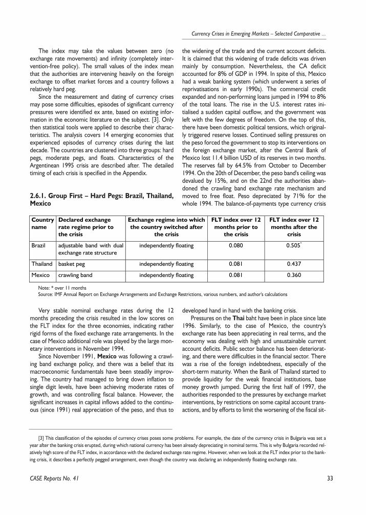
33
Currency Crises in Emerging Markets – Selected Comparative ...
The index may take the values between zero (noexchange rate movements) and infinity (completely inter-vention-free policy). The small values of the index meanthat the authorities are intervening heavily on the foreignexchange to offset market forces and a country follows arelatively hard peg.
Since the measurement and dating of currency crisesmay pose some difficulties, episodes of significant currencypressures were identified ex ante, based on existing infor-mation in the economic literature on the subject. [3]. Onlythen statistical tools were applied to describe their charac-teristics. The analysis covers 14 emerging economies thatexperienced episodes of currency crises during the lastdecade. The countries are clustered into three groups: hardpegs, moderate pegs, and floats. Characteristics of theArgentinean 1995 crisis are described after. The detailedtiming of each crisis is specified in the Appendix.
2.6.1. Group First – Hard Pegs: Brazil, Thailand,Mexico
Very stable nominal exchange rates during the 12months preceding the crisis resulted in the low scores onthe FLT index for the three economies, indicating ratherrigid forms of the fixed exchange rate arrangements. In thecase of Mexico additional role was played by the large mon-etary interventions in November 1994.
Since November 1991, Mexico was following a crawl-ing band exchange policy, and there was a belief that itsmacroeconomic fundamentals have been steadily improv-ing. The country had managed to bring down inflation tosingle digit levels, have been achieving moderate rates ofgrowth, and was controlling fiscal balance. However, thesignificant increases in capital inflows added to the continu-ous (since 1991) real appreciation of the peso, and thus to
the widening of the trade and the current account deficits.It is claimed that this widening of trade deficits was drivenmainly by consumption. Nevertheless, the CA deficitaccounted for 8% of GDP in 1994. In spite of this, Mexicohad a weak banking system (which underwent a series ofreprivatisations in early 1990s). The commercial creditexpanded and non-performing loans jumped in 1994 to 8%of the total loans. The rise in the U.S. interest rates ini-tialised a sudden capital outflow, and the government wasleft with the few degrees of freedom. On the top of this,there have been domestic political tensions, which original-ly triggered reserve losses. Continued selling pressures onthe peso forced the government to stop its interventions onthe foreign exchange market, after the Central Bank ofMexico lost 11.4 billion USD of its reserves in two months.The reserves fall by 64.5% from October to December1994. On the 20th of December, the peso band's ceiling wasdevalued by 15%, and on the 22nd the authorities aban-doned the crawling band exchange rate mechanism andmoved to free float. Peso depreciated by 71% for thewhole 1994. The balance-of-payments type currency crisis
developed hand in hand with the banking crisis.Pressures on the Thai baht have been in place since late
1996. Similarly, to the case of Mexico, the country'sexchange rate has been appreciating in real terms, and theeconomy was dealing with high and unsustainable currentaccount deficits. Public sector balance has been deteriorat-ing, and there were difficulties in the financial sector. Therewas a rise of the foreign indebtedness, especially of theshort-term maturity. When the Bank of Thailand started toprovide liquidity for the weak financial institutions, basemoney growth jumped. During the first half of 1997, theauthorities responded to the pressures by exchange marketinterventions, by restrictions on some capital account trans-actions, and by efforts to limit the worsening of the fiscal sit-
CASE Reports No. 41
Countryname
Declared exchangerate regime prior tothe crisis
Exchange regime into whichthe country switched after
the crisis
FLT index over 12months prior to
the crisis
FLT index over 12months after the
crisis
Brazil adjustable band with dualexchange rate structure
independently floating 0.080 0.505*
Thailand basket peg independently floating 0.081 0.437
Mexico crawling band independently floating 0.081 0.360
Note: * over 11 monthsSource: IMF Annual Report on Exchange Arrangements and Exchange Restrictions, various numbers, and author's calculations
[3] This classification of the episodes of currency crises poses some problems. For example, the date of the currency crisis in Bulgaria was set ayear after the banking crisis erupted, during which national currency has been already depreciating in nominal terms. This is why Bulgaria recorded rel-atively high score of the FLT index, in accordance with the declared exchange rate regime. However, when we look at the FLT index prior to the bank-ing crisis, it describes a perfectly pegged arrangement, even though the country was declaring an independently floating exchange rate.
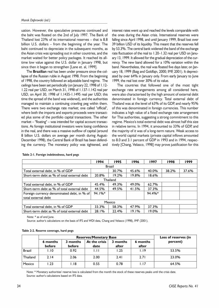
34
Marek D¹browski (ed.)
uation. However, the speculative pressures continued andthe baht was floated on the 2nd of July 1997. The Bank ofThailand lost 23% of its international reserves – that is 8.8billion U.S. dollars – from the beginning of the year. Thebaht continued to depreciate in the subsequent months, asthe Asian crisis was spreading out in other countries, and themarket waited for better policy packages. It reached its all-time low value against the U.S. dollar in January 1998, butsince then it began to strengthen [Lane et. al, 1999].
The Brazilian real has been under pressure since the col-lapse of the Russian ruble in August 1998. From the beginningof 1998, the country followed an adjustable band regime. Theceilings have been set periodically (on January 22, 1998 of 1.12-1.22 real per USD, on March 31, 1998 of 1.137-1.142 real perUSD, on April 30, 1998 of 1.1435-1.1495 real per USD; thistime the spread of the band was widened), and the authoritiesmanaged to maintain a continuing crawling peg within them.There were two exchange rate market; one called "official",where both the imports and exports proceeds were transact-ed plus some of the portfolio capital transactions. The othermarket – "floating" – was intended for capital account transac-tions. As foreign institutional investors were losing confidencein the real, and there was a massive outflow of capital (around8 billion U.S. dollars on average per month during August-December 1998), the Central Bank of Brazil has been defend-ing the currency. The monetary policy was tightened, and
interest rates went up and reached the levels comparable withthe ones during the Asian crisis. International reserves werefalling since April 1998, and until January 1999, Brazil lost over39 billion USD of its liquidity. This meant that the reserves fellby 53.3%. The central bank widened the band of the exchangerate fluctuation of the real to 1.20–1.32 real per USD on Janu-ary 13, 1999. It allowed for the gradual depreciation of the cur-rency. The new band allowed for a 10% variation within theband. Nevertheless, the real was floated five days later, on Jan-uary 18, 1999 (Baig and Goldfajn, 2000; IMF, 2001). It depreci-ated by over 64% in January only. From early January to June1999, the real lost over 30% of its value.
The countries that followed one of the most tightexchange rate arrangements among all considered here,were also characterised by the high amount of external debtdenominated in foreign currency. Total external debt ofThailand was at the level of 63% of its GDP, and nearly 95%of this was denominated in foreign currencies. This numberindicates a high value of a fixed exchange rate arrangementfor Thai authorities, suggesting a strong commitment to thisregime. Mexico's total external debt was almost half this sizein relative terms. In 1994, it amounted to 33% of GDP, andthe majority of it was of a long-term nature. Weak access tothe world capital markets (private capital inflows amountedto 8.0 and 3.1 percent of GDP in 1993 and in 1994, respec-tively [Chang, Velasco, 1998] may prove justification for this
CASE Reports No. 41
Table 2-2. Reserve coverage, hard pegs
Reserves/Monetary Base6 months
before3 months
beforeAt the crisis
date3 months
after6 months
after
Loss of reserves (inpercent)
Brazil 1.10 0.92 1.11 1.25 1.19 53.5%
Thailand 2.14 2.06 2.00 2.41 2.71 23.0%
Mexico 1.23 1.18 0.55 0.78 1.17 64.5%
Note: * Monetary authorities' reserve loss is calculated from the month the stock of these reserves peaks until the crisis date.Source: author's calculations based on IFS data.
Table 2-1. Foreign indebtedness, hard pegs
1994 1995 1996 1997 1998 1999Brazil
Total external debt, in % of GDP 30.7% 45.6% 40.0% 38.2% 37.6%Short-term debt as % of total external debt 20.8% 19.2% 19.8% 18.6%
ThailandTotal external debt, in % of GDP 45.4% 49.3% 49.0% 62.7%Short-term debt as % of total external debt 44.5% 49.5% 41.5% 37.3%Foreign currency denominated debt, in % oftotal external debt
94.1%* 94.4%*
MexicoTotal external debt, in % of GDP 33.3% 58.3% 47.9% 37.3%Short-term debt as % of total external debt 28.1% 22.4% 19.1% 19.0%
Note: * as of end June.Source: author's calculations on the basis of IFS and WDI data, Chang and Velasco (1998), IMF (2001).

35
Currency Crises in Emerging Markets – Selected Comparative ...
regime choice. Total external debt of Brazil amounted to38% of GDP in 1998–1999, while outstanding external debtrose from 23% in 1996 to 45% of GDP in 1999.
While these economies were defending values of theircurrencies, they lost large amounts of internationalreserves. When we compare the percentage reserve loss atthe crisis dates of all of the countries described here, it isclear that Mexico and Brazil lost the most.
If we were to asses costs and advantages associated withthe decision of quitting the peg of these countries, thereseems to be a reason in abandoning the fixed arrangementin Thailand and Mexico, in the sense that continuationwould have became too expensive. Mexico's internationalreserves were not even covering half of its short-termexternal debt. Thailand had a level of reserves roughly equalthe amount of its short-term debt 3 months before thedevaluation, but was losing its reserves quickly, so that inJune 1997 the reserves to its short-term external debt ratiowas 0.85. Relevant ratio for Brazil was not that bad, butwhen we look at the more precise indicator of grossreserves to the residual maturity at the end of 1998, it isclear that reserves were covering only 53% of the debt.
Both Brazil and Thailand allowed its currencies to float,and tightened monetary policies, avoiding inflation-depreci-ation spirals. These moves were costly for the real econo-my, but it seems that the alternatives would have beenmuch more expensive. However, this was not the case ofMexico, where there was a passthrough of depreciation onprices, but nevertheless, the economy returned to itsgrowth path about a year after the crisis.
2.6.2. Group Second – Moderate Pegs: Russia,Georgia, Ukraine, Korea, Indonesia, Malaysia,Moldova
This classification groups seven countries that declareddifferent types of their exchange rate regimes before thecrisis. Even if they officially did not change their declaredarrangements after the crises, they certainly allowed for agreater flexibility of their exchange rates over at least oneyear after.
From all Asian economies hit by the crisis, Koreaappeared initially to be less affected. From 1993 the coun-try followed an exchange rate band, with the currencyfixed to the U.S. dollar, and won managed to oscillate with-in the permitted range of fluctuations of +/- 2%. Theexchange rate remained broadly stable until October 1997.However, the country had a large stock of debt of shortmaturity, and its international reserves were only moder-ate. The macroeconomic fundamentals remained generallyfavourable but the financial institutions and large corpora-tions began to experience problems earlier this year. As thecrisis was spreading out, external financing conditionsbegun to worsen, and the won fell by over 5%. Theauthority started to intervene, but the reserves weredepleted very quickly. Monetary policy was tightened, butsoon released because of its impact on the highly leveragedcorporate sector. By December 1997, won depreciated byover 20% against U.S. dollar, and usable foreign reservesfell to 6 billion U.S. dollars; from over 22 billions at the endof October 1997 [Lane et al., 1999]. Balino and Ubida(1999) write that at the end of 1997 usable foreign reserveswere at the level equal to 0.6 month of imports. One yearearlier, the reserves amounted to 2 months of imports. Theexchange rate was allowed to float freely on December 16,1997, and reached its lowest value against the dollar onDecember 23, 1997 [Balino, Ubida, 1999]. By mid-1998won remained generally stable after the initial appreciationin January and the country made progress towards over-coming financial crisis.
CASE Reports No. 41
Countryname
Declared exchangerate regime prior to
the crisis
Exchange regime intowhich the countryswitched after the
crisis
FLT index over 12months prior to the
crisis
FLT index over 12months after the crisis
Russia exchange rate band managed float 0.124 1.093
Georgia conventional peg independently floating 0.185 0.566
Ukraine horizontal band horizontal band 0.202 0.558
Korea exchange rate band independently floating 0.256* 0.530
Indonesia crawling band independently floating 0.271 0.495
Malaysia managed float managed float** 0.285 1.221
Moldova managed float independently floating 0.358 0.672
Note: * counted back form the beginning of the Thai crisis. It is commonly agreed that the crisis in Korea erupted in December 1997, but won wasunder serious pressure form the summer of 1997. For this reason period from July to November 1997 was excluded from the pre-crisis calculations.
** Malaysia switched to the conventional peg arrangement in September 1998, a year after the currency crisis started.Source: IMF Annual Report on Exchange Arrangements and Exchange Restrictions, various numbers, and author's calculations
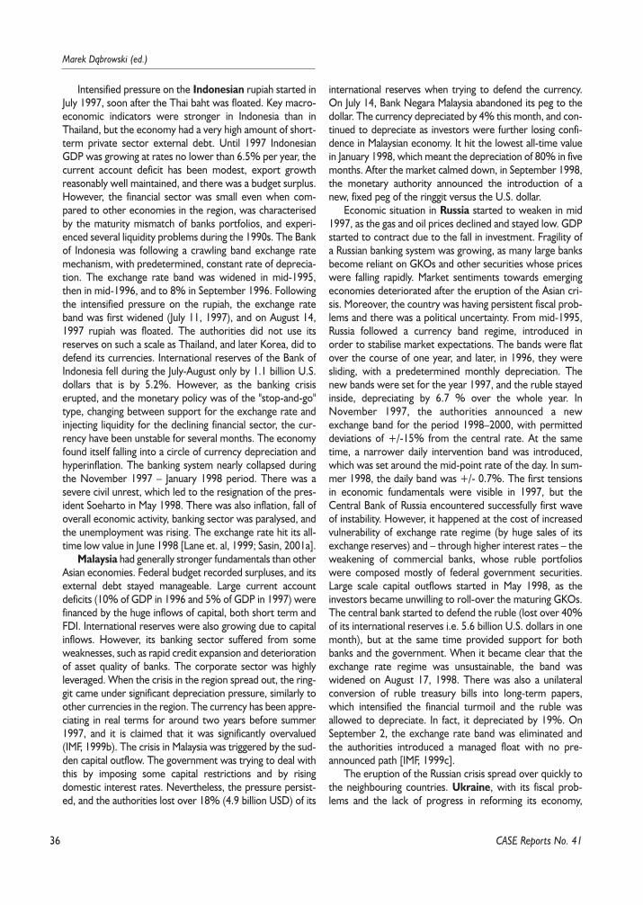
36
Marek D¹browski (ed.)
Intensified pressure on the Indonesian rupiah started inJuly 1997, soon after the Thai baht was floated. Key macro-economic indicators were stronger in Indonesia than inThailand, but the economy had a very high amount of short-term private sector external debt. Until 1997 IndonesianGDP was growing at rates no lower than 6.5% per year, thecurrent account deficit has been modest, export growthreasonably well maintained, and there was a budget surplus.However, the financial sector was small even when com-pared to other economies in the region, was characterisedby the maturity mismatch of banks portfolios, and experi-enced several liquidity problems during the 1990s. The Bankof Indonesia was following a crawling band exchange ratemechanism, with predetermined, constant rate of deprecia-tion. The exchange rate band was widened in mid-1995,then in mid-1996, and to 8% in September 1996. Followingthe intensified pressure on the rupiah, the exchange rateband was first widened (July 11, 1997), and on August 14,1997 rupiah was floated. The authorities did not use itsreserves on such a scale as Thailand, and later Korea, did todefend its currencies. International reserves of the Bank ofIndonesia fell during the July-August only by 1.1 billion U.S.dollars that is by 5.2%. However, as the banking crisiserupted, and the monetary policy was of the "stop-and-go"type, changing between support for the exchange rate andinjecting liquidity for the declining financial sector, the cur-rency have been unstable for several months. The economyfound itself falling into a circle of currency depreciation andhyperinflation. The banking system nearly collapsed duringthe November 1997 – January 1998 period. There was asevere civil unrest, which led to the resignation of the pres-ident Soeharto in May 1998. There was also inflation, fall ofoverall economic activity, banking sector was paralysed, andthe unemployment was rising. The exchange rate hit its all-time low value in June 1998 [Lane et. al, 1999; Sasin, 2001a].
Malaysia had generally stronger fundamentals than otherAsian economies. Federal budget recorded surpluses, and itsexternal debt stayed manageable. Large current accountdeficits (10% of GDP in 1996 and 5% of GDP in 1997) werefinanced by the huge inflows of capital, both short term andFDI. International reserves were also growing due to capitalinflows. However, its banking sector suffered from someweaknesses, such as rapid credit expansion and deteriorationof asset quality of banks. The corporate sector was highlyleveraged. When the crisis in the region spread out, the ring-git came under significant depreciation pressure, similarly toother currencies in the region. The currency has been appre-ciating in real terms for around two years before summer1997, and it is claimed that it was significantly overvalued(IMF, 1999b). The crisis in Malaysia was triggered by the sud-den capital outflow. The government was trying to deal withthis by imposing some capital restrictions and by risingdomestic interest rates. Nevertheless, the pressure persist-ed, and the authorities lost over 18% (4.9 billion USD) of its
international reserves when trying to defend the currency.On July 14, Bank Negara Malaysia abandoned its peg to thedollar. The currency depreciated by 4% this month, and con-tinued to depreciate as investors were further losing confi-dence in Malaysian economy. It hit the lowest all-time valuein January 1998, which meant the depreciation of 80% in fivemonths. After the market calmed down, in September 1998,the monetary authority announced the introduction of anew, fixed peg of the ringgit versus the U.S. dollar.
Economic situation in Russia started to weaken in mid1997, as the gas and oil prices declined and stayed low. GDPstarted to contract due to the fall in investment. Fragility ofa Russian banking system was growing, as many large banksbecome reliant on GKOs and other securities whose priceswere falling rapidly. Market sentiments towards emergingeconomies deteriorated after the eruption of the Asian cri-sis. Moreover, the country was having persistent fiscal prob-lems and there was a political uncertainty. From mid-1995,Russia followed a currency band regime, introduced inorder to stabilise market expectations. The bands were flatover the course of one year, and later, in 1996, they weresliding, with a predetermined monthly depreciation. Thenew bands were set for the year 1997, and the ruble stayedinside, depreciating by 6.7 % over the whole year. InNovember 1997, the authorities announced a newexchange band for the period 1998–2000, with permitteddeviations of +/-15% from the central rate. At the sametime, a narrower daily intervention band was introduced,which was set around the mid-point rate of the day. In sum-mer 1998, the daily band was +/- 0.7%. The first tensionsin economic fundamentals were visible in 1997, but theCentral Bank of Russia encountered successfully first waveof instability. However, it happened at the cost of increasedvulnerability of exchange rate regime (by huge sales of itsexchange reserves) and – through higher interest rates – theweakening of commercial banks, whose ruble portfolioswere composed mostly of federal government securities.Large scale capital outflows started in May 1998, as theinvestors became unwilling to roll-over the maturing GKOs.The central bank started to defend the ruble (lost over 40%of its international reserves i.e. 5.6 billion U.S. dollars in onemonth), but at the same time provided support for bothbanks and the government. When it became clear that theexchange rate regime was unsustainable, the band waswidened on August 17, 1998. There was also a unilateralconversion of ruble treasury bills into long-term papers,which intensified the financial turmoil and the ruble wasallowed to depreciate. In fact, it depreciated by 19%. OnSeptember 2, the exchange rate band was eliminated andthe authorities introduced a managed float with no pre-announced path [IMF, 1999c].
The eruption of the Russian crisis spread over quickly tothe neighbouring countries. Ukraine, with its fiscal prob-lems and the lack of progress in reforming its economy,
CASE Reports No. 41
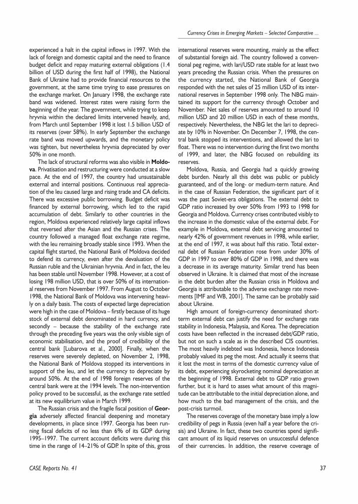
37
Currency Crises in Emerging Markets – Selected Comparative ...
experienced a halt in the capital inflows in 1997. With thelack of foreign and domestic capital and the need to financebudget deficit and repay maturing external obligations (1.4billion of USD during the first half of 1998), the NationalBank of Ukraine had to provide financial resources to thegovernment, at the same time trying to ease pressures onthe exchange market. On January 1998, the exchange rateband was widened. Interest rates were raising form thebeginning of the year. The government, while trying to keephryvnia within the declared limits intervened heavily, and,from March until September 1998 it lost 1.5 billion USD ofits reserves (over 58%). In early September the exchangerate band was moved upwards, and the monetary policywas tighten, but nevertheless hryvnia depreciated by over50% in one month.
The lack of structural reforms was also visible in Moldo-va. Privatisation and restructuring were conducted at a slowpace. At the end of 1997, the country had unsustainableexternal and internal positions. Continuous real apprecia-tion of the leu caused large and rising trade and CA deficits.There was excessive public borrowing. Budget deficit wasfinanced by external borrowing, which led to the rapidaccumulation of debt. Similarly to other countries in theregion, Moldova experienced relatively large capital inflowsthat reversed after the Asian and the Russian crises. Thecountry followed a managed float exchange rate regime,with the leu remaining broadly stable since 1993. When thecapital flight started, the National Bank of Moldova decidedto defend its currency, even after the devaluation of theRussian ruble and the Ukrainian hryvnia. And in fact, the leuhas been stable until November 1998. However, at a cost oflosing 198 million USD, that is over 50% of its internation-al reserves from November 1997. From August to October1998, the National Bank of Moldova was intervening heavi-ly on a daily basis. The costs of expected large depreciationwere high in the case of Moldova – firstly because of its hugestock of external debt denominated in hard currency, andsecondly – because the stability of the exchange ratethrough the preceding five years was the only visible sign ofeconomic stabilisation, and the proof of credibility of thecentral bank [Lubarova et al., 2000]. Finally, when thereserves were severely depleted, on November 2, 1998,the National Bank of Moldova stopped its interventions insupport of the leu, and let the currency to depreciate byaround 50%. At the end of 1998 foreign reserves of thecentral bank were at the 1994 levels. The non-interventionpolicy proved to be successful, as the exchange rate settledat its new equilibrium value in March 1999.
The Russian crisis and the fragile fiscal position of Geor-gia adversely affected financial deepening and monetarydevelopments, in place since 1997. Georgia has been run-ning fiscal deficits of no less than 6% of its GDP during1995–1997. The current account deficits were during thistime in the range of 14–21% of GDP. In spite of this, gross
international reserves were mounting, mainly as the effectof substantial foreign aid. The country followed a conven-tional peg regime, with lari/USD rate stable for at least twoyears preceding the Russian crisis. When the pressures onthe currency started, the National Bank of Georgiaresponded with the net sales of 25 million USD of its inter-national reserves in September 1998 only. The NBG main-tained its support for the currency through October andNovember. Net sales of reserves amounted to around 10million USD and 20 million USD in each of these months,respectively. Nevertheless, the NBG let the lari to depreci-ate by 10% in November. On December 7, 1998, the cen-tral bank stopped its interventions, and allowed the lari tofloat. There was no intervention during the first two monthsof 1999, and later, the NBG focused on rebuilding itsreserves.
Moldova, Russia, and Georgia had a quickly growingdebt burden. Nearly all this debt was public or publiclyguaranteed, and of the long- or medium-term nature. Andin the case of Russian Federation, the significant part of itwas the past Soviet-era obligations. The external debt toGDP ratio increased by over 50% from 1993 to 1998 forGeorgia and Moldova. Currency crises contributed visibly tothe increase in the domestic value of the external debt. Forexample in Moldova, external debt servicing amounted tonearly 42% of government revenues in 1998, while earlier,at the end of 1997, it was about half this ratio. Total exter-nal debt of Russian Federation rose from under 30% ofGDP in 1997 to over 80% of GDP in 1998, and there wasa decrease in its average maturity. Similar trend has beenobserved in Ukraine. It is claimed that most of the increasein the debt burden after the Russian crisis in Moldova andGeorgia is attributable to the adverse exchange rate move-ments [IMF and WB, 2001]. The same can be probably saidabout Ukraine.
High amount of foreign-currency denominated short-term external debt can justify the need for exchange ratestability in Indonesia, Malaysia, and Korea. The depreciationcosts have been reflected in the increased debt/GDP ratio,but not on such a scale as in the described CIS countries.The most heavily indebted was Indonesia, hence Indonesiaprobably valued its peg the most. And actually it seems thatit lost the most in terms of the domestic currency value ofits debt, experiencing skyrocketing nominal depreciation atthe beginning of 1998. External debt to GDP ratio grownfurther, but it is hard to asses what amount of this magni-tude can be attributable to the initial depreciation alone, andhow much to the bad management of the crisis, and thepost-crisis turmoil.
The reserves coverage of the monetary base imply a lowcredibility of pegs in Russia (even half a year before the cri-sis) and Ukraine. In fact, these two countries spend signifi-cant amount of its liquid reserves on unsuccessful defenceof their currencies. In addition, the reserve coverage of
CASE Reports No. 41
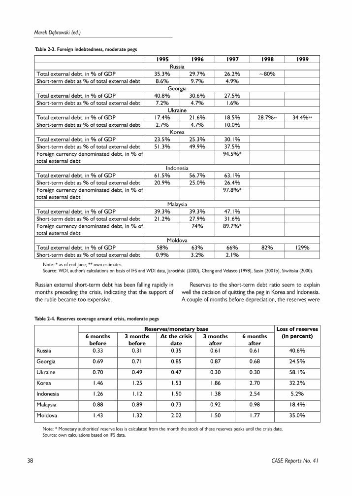
Russian external short-term debt has been falling rapidly inmonths preceding the crisis, indicating that the support ofthe ruble became too expensive.
Reserves to the short-term debt ratio seem to explainwell the decision of quitting the peg in Korea and Indonesia.A couple of months before depreciation, the reserves were
38
Marek D¹browski (ed.)
CASE Reports No. 41
Table 2-3. Foreign indebtedness, moderate pegs
1995 1996 1997 1998 1999Russia
Total external debt, in % of GDP 35.3% 29.7% 26.2% ~80%Short-term debt as % of total external debt 8.6% 9.7% 4.9%
GeorgiaTotal external debt, in % of GDP 40.8% 30.6% 27.5%Short-term debt as % of total external debt 7.2% 4.7% 1.6%
UkraineTotal external debt, in % of GDP 17.4% 21.6% 18.5% 28.7%** 34.4%**
Short-term debt as % of total external debt 2.7% 4.7% 10.0%Korea
Total external debt, in % of GDP 23.5% 25.3% 30.1%Short-term debt as % of total external debt 51.3% 49.9% 37.5%Foreign currency denominated debt, in % oftotal external debt
94.5%*
IndonesiaTotal external debt, in % of GDP 61.5% 56.7% 63.1%Short-term debt as % of total external debt 20.9% 25.0% 26.4%Foreign currency denominated debt, in % oftotal external debt
97.8%*
MalaysiaTotal external debt, in % of GDP 39.3% 39.3% 47.1%Short-term debt as % of total external debt 21.2% 27.9% 31.6%Foreign currency denominated debt, in % oftotal external debt
74% 89.7%*
MoldovaTotal external debt, in % of GDP 58% 63% 66% 82% 129%Short-term debt as % of total external debt 0.9% 3.2% 2.1%
Note: * as of end June; ** own estimates.Source: WDI, author's calculations on basis of IFS and WDI data, Jarociñski (2000), Chang and Velasco (1998), Sasin (2001b), Siwiñska (2000).
Table 2-4. Reserves coverage around crisis, moderate pegs
Reserves/monetary base6 months
before3 months
beforeAt the crisis
date3 months
after6 months
after
Loss of reserves(in percent)
Russia 0.33 0.31 0.35 0.61 0.61 40.6%
Georgia 0.69 0.71 0.85 0.87 0.68 24.5%
Ukraine 0.70 0.49 0.47 0.30 0.30 58.1%
Korea 1.46 1.25 1.53 1.86 2.70 32.2%
Indonesia 1.26 1.12 1.50 1.38 2.54 5.2%
Malaysia 0.88 0.89 0.73 0.92 0.98 18.4%
Moldova 1.43 1.32 2.02 1.50 1.77 35.0%
Note: * Monetary authorities' reserve loss is calculated from the month the stock of these reserves peaks until the crisis date.Source: own calculations based on IFS data.
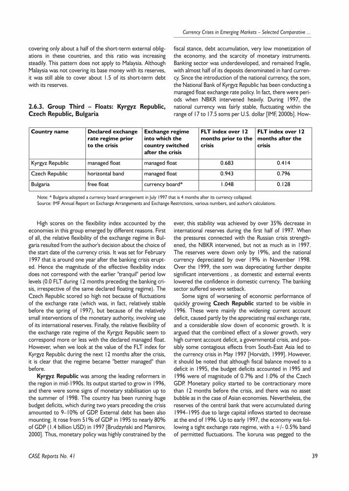
39
Currency Crises in Emerging Markets – Selected Comparative ...
covering only about a half of the short-term external oblig-ations in these countries, and this ratio was increasingsteadily. This pattern does not apply to Malaysia. AlthoughMalaysia was not covering its base money with its reserves,it was still able to cover about 1.5 of its short-term debtwith its reserves.
2.6.3. Group Third – Floats: Kyrgyz Republic,Czech Republic, Bulgaria
High scores on the flexibility index accounted by theeconomies in this group emerged by different reasons. Firstof all, the relative flexibility of the exchange regime in Bul-garia resulted from the author's decision about the choice ofthe start date of the currency crisis. It was set for February1997 that is around one year after the banking crisis erupt-ed. Hence the magnitude of the effective flexibility indexdoes not correspond with the earlier "tranquil" period lowlevels (0.0 FLT during 12 months preceding the banking cri-sis, irrespective of the same declared floating regime). TheCzech Republic scored so high not because of fluctuationsof the exchange rate (which was, in fact, relatively stablebefore the spring of 1997), but because of the relativelysmall interventions of the monetary authority, involving useof its international reserves. Finally, the relative flexibility ofthe exchange rate regime of the Kyrgyz Republic seem tocorrespond more or less with the declared managed float.However, when we look at the value of the FLT index forKyrgyz Republic during the next 12 months after the crisis,it is clear that the regime became "better managed" thanbefore.
Kyrgyz Republic was among the leading reformers inthe region in mid-1990s. Its output started to grow in 1996,and there were some signs of monetary stabilisation up tothe summer of 1998. The country has been running hugebudget deficits, which during two years preceding the crisisamounted to 9–10% of GDP. External debt has been alsomounting. It rose from 51% of GDP in 1995 to nearly 80%of GDP (1.4 billion USD) in 1997 [Brudzyñski and Mamirov,2000]. Thus, monetary policy was highly constrained by the
fiscal stance, debt accumulation, very low monetization ofthe economy, and the scarcity of monetary instruments.Banking sector was underdeveloped, and remained fragile,with almost half of its deposits denominated in hard curren-cy. Since the introduction of the national currency, the som,the National Bank of Kyrgyz Republic has been conducting amanaged float exchange rate policy. In fact, there were peri-ods when NBKR intervened heavily. During 1997, thenational currency was fairly stable, fluctuating within therange of 17 to 17.5 soms per U.S. dollar [IMF, 2000b]. How-
ever, this stability was achieved by over 35% decrease ininternational reserves during the first half of 1997. Whenthe pressures connected with the Russian crisis strength-ened, the NBKR intervened, but not as much as in 1997.The reserves were down only by 19%, and the nationalcurrency depreciated by over 19% in November 1998.Over the 1999, the som was depreciating further despitesignificant interventions , as domestic and external eventslowered the confidence in domestic currency. The bankingsector suffered severe setback.
Some signs of worsening of economic performance ofquickly growing Czech Republic started to be visible in1996. These were mainly the widening current accountdeficit, caused partly by the appreciating real exchange rate,and a considerable slow down of economic growth. It isargued that the combined effect of a slower growth, veryhigh current account deficit, a governmental crisis, and pos-sibly some contagious effects from South-East Asia led tothe currency crisis in May 1997 [Horváth, 1999]. However,it should be noted that although fiscal balance moved to adeficit in 1995, the budget deficits accounted in 1995 and1996 were of magnitude of 0.7% and 1.0% of the CzechGDP. Monetary policy started to be contractionary morethan 12 months before the crisis, and there was no assetbubble as in the case of Asian economies. Nevertheless, thereserves of the central bank that were accumulated during1994–1995 due to large capital inflows started to decreaseat the end of 1996. Up to early 1997, the economy was fol-lowing a tight exchange rate regime, with a +/- 0.5% bandof permitted fluctuations. The koruna was pegged to the
CASE Reports No. 41
Country name Declared exchangerate regime priorto the crisis
Exchange regimeinto which thecountry switchedafter the crisis
FLT index over 12months prior to thecrisis
FLT index over 12months after thecrisis
Kyrgyz Republic managed float managed float 0.683 0.414
Czech Republic horizontal band managed float 0.943 0.796
Bulgaria free float currency board* 1.048 0.128
Note: * Bulgaria adopted a currency board arrangement in July 1997 that is 4 months after its currency collapsed.Source: IMF Annual Report on Exchange Arrangements and Exchange Restrictions, various numbers, and author's calculations.
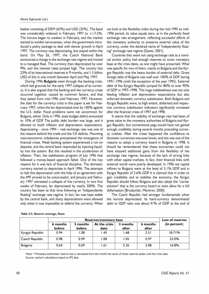
40
Marek D¹browski (ed.)
basket consisting of DEM (65%) and USD (35%). The bandwas considerably widened in February 1997 to +/-7.5%.The koruna began to weaken in February, and the marketstarted to exhibit nervousness, when the government intro-duced a policy package to deal with slower growth in April1997. The currency was depreciating, but stayed within theband. On May 26, 1997, the Czech National Bankannounced a change in the exchange rate regime and movedto a managed float. The currency then depreciated by over9%, and the interest rates jumped high. The country lost23% of its international reserves in 9 months, and 1.5 billionUSD of this in one month between April and May 1997.
During 1996 Bulgaria went through the banking crisis,which laid grounds for the early 1997 collapse of its curren-cy. It is also argued that the banking and the currency crisesoccurred together, caused by common factors, and thatthey lasted from mid-1996 until February 1997. However,the date for the currency crisis in this paper is set for Feb-ruary 1997, when the lev depreciated over by 100% againstthe U.S. dollar. Fiscal problems were not uncommon forBulgaria, either. Only in 1996, state budget deficit amountedto 10% of GDP. The public debt burden was large, and itallowed to build inflation and depreciation expectations.Appreciating – since 1994 – real exchange rate was one ofthe reasons behind the trade and the CA deficits. Mountingmacroeconomic imbalances precipitated the emergence offinancial crises. Weak banking system experienced a run ondeposits, and the central bank responded by injecting liquid-ity into the system. But this resulted in the acceleration ofinflation. Then, the stabilisation program of July 1996 thatfollowed a money-based approach failed. One of the keyreasons for it was lack of financial discipline. The domesticcurrency started to depreciate in April 1996. The attemptsto halt this depreciation with the help of an agreement withthe IMF proved to be unsuccessful, and January and Febru-ary 1997 witnessed a collapse of the currency. In two firstweeks of February, lev depreciated by nearly 200%. Thecountry has been at that time following an "independentlyfloating" exchange rate regime. In fact, lev was kept stableby the central bank, and sharp depreciations were allowedonly when it was impossible to defend the currency. When
we look at the flexibility index during the mid-1995 to mid-1996 period, its value equals zero, as in the perfectly fixedexchange rate arrangement, reflecting successful efforts ofthe monetary authority to preserve external value of thecurrency, under the declared name of "independently float-ing" exchange rate regime [Ganev, 2001].
Countries that were not using exchange rate as a nomi-nal anchor policy had enough reserves to cover monetarybase at the crisis dates, as one might have presumed. Whatwas specific for two of them, mainly to Bulgaria and the Kyr-gyz Republic was the heavy burden of external debt. Grossforeign debt of Bulgaria was well over 100% of GDP during1991–1996 (with the exception of the year 1995). Externaldebt of the Kyrgyz Republic jumped for 80% to over 90%of GDP in 1997–1998. This huge indebtedness was not onlyfeeding inflation and depreciation expectations but alsoenforced domestic currency substitution. Both Bulgaria andKyrgyz Republic were, to high extent, dollarised and respec-tive currency substitution indicators significantly increasedafter the financial crises of 1997 and 1998.
It seems that the stability of exchange rate had been ofgreat value to the monetary authorities of Bulgaria and Kyr-gyz Republic, but conventional pegs would have not gainedenough credibility during several months preceding curren-cy crashes. After the crises happened the confidence todomestic currencies was even lower, and this was one of thereasons to adopt a currency board in Bulgaria in 1998. Itshould be remembered that these economies could nothave enjoyed additional gains from the flexibility of theexchange rate regime, because of the lack of strong linkswith other capital markets. In fact, their financial links withexternal world were poorly developed. In 1996 net capitalinflows to Bulgaria were at the level of 3.1% GDP, and inKyrgyz Republic of 2.6% GDP. It is claimed that in order togain credibility and to stabilise the economy, the KyrgyzRepublic should follow Bulgaria and also adopt the "cornersolution" that is the currency board or even allow for a fulldollarisation [Brudzyñski, Mamirov, 2000].
The Czech Republic had stronger fundamentals whenthe koruna depreciated. Its hard-currency denominateddebt to GDP ratio was about 41% of GDP at the end of
CASE Reports No. 41
Table 2-5. Reserve coverage, floats
Reserves/monetary base6 months
before3 months
beforeAt the crisis
date3 months
after6 months
after
Loss of reserves(in percent)
Kyrgyz Republic 0.94 1.08 1.45 1.68 2.51 18.71%
Czech Republic 0.98 0.99 1.08 1.05 0.97 23.0%
Bulgaria 0.64 0.69 1.61 2.36 2.08 16.8%
Note: * Monetary authorities' reserve loss is calculated from the month the stock of these reserves peaks until the crisis dateSource: author's calculations based on IFS data
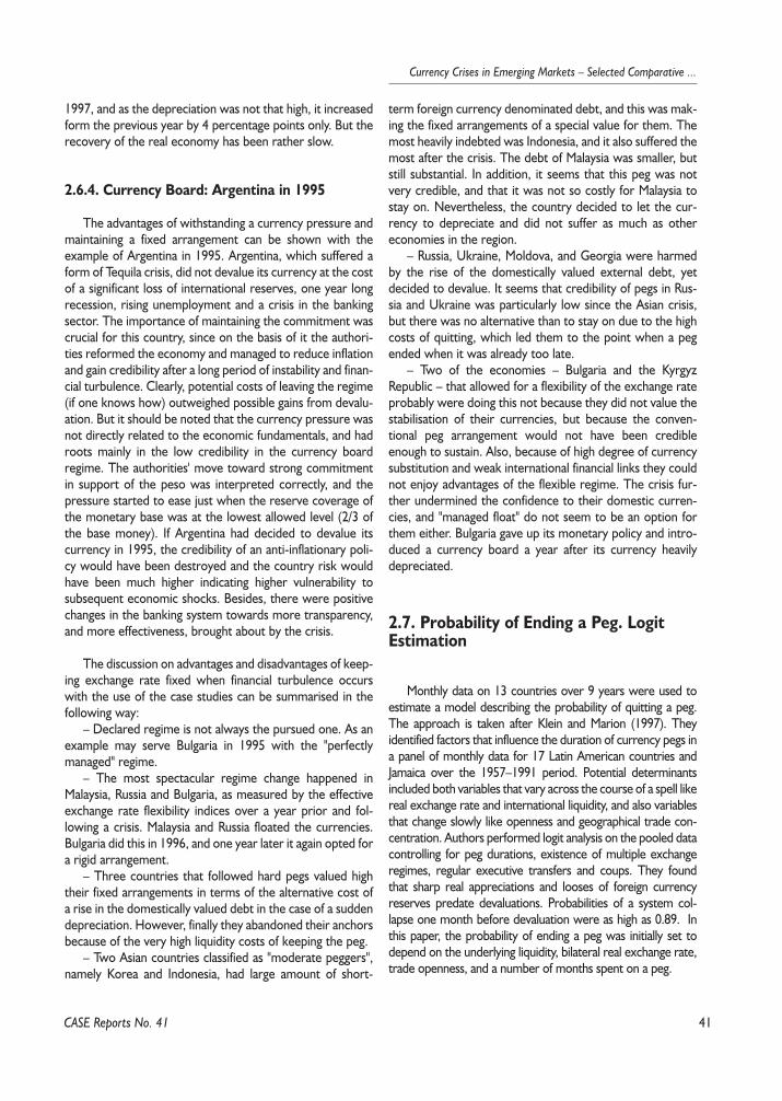
41
Currency Crises in Emerging Markets – Selected Comparative ...
CASE Reports No. 41
1997, and as the depreciation was not that high, it increasedform the previous year by 4 percentage points only. But therecovery of the real economy has been rather slow.
2.6.4. Currency Board: Argentina in 1995
The advantages of withstanding a currency pressure andmaintaining a fixed arrangement can be shown with theexample of Argentina in 1995. Argentina, which suffered aform of Tequila crisis, did not devalue its currency at the costof a significant loss of international reserves, one year longrecession, rising unemployment and a crisis in the bankingsector. The importance of maintaining the commitment wascrucial for this country, since on the basis of it the authori-ties reformed the economy and managed to reduce inflationand gain credibility after a long period of instability and finan-cial turbulence. Clearly, potential costs of leaving the regime(if one knows how) outweighed possible gains from devalu-ation. But it should be noted that the currency pressure wasnot directly related to the economic fundamentals, and hadroots mainly in the low credibility in the currency boardregime. The authorities' move toward strong commitmentin support of the peso was interpreted correctly, and thepressure started to ease just when the reserve coverage ofthe monetary base was at the lowest allowed level (2/3 ofthe base money). If Argentina had decided to devalue itscurrency in 1995, the credibility of an anti-inflationary poli-cy would have been destroyed and the country risk wouldhave been much higher indicating higher vulnerability tosubsequent economic shocks. Besides, there were positivechanges in the banking system towards more transparency,and more effectiveness, brought about by the crisis.
The discussion on advantages and disadvantages of keep-ing exchange rate fixed when financial turbulence occurswith the use of the case studies can be summarised in thefollowing way:
– Declared regime is not always the pursued one. As anexample may serve Bulgaria in 1995 with the "perfectlymanaged" regime.
– The most spectacular regime change happened inMalaysia, Russia and Bulgaria, as measured by the effectiveexchange rate flexibility indices over a year prior and fol-lowing a crisis. Malaysia and Russia floated the currencies.Bulgaria did this in 1996, and one year later it again opted fora rigid arrangement.
– Three countries that followed hard pegs valued hightheir fixed arrangements in terms of the alternative cost ofa rise in the domestically valued debt in the case of a suddendepreciation. However, finally they abandoned their anchorsbecause of the very high liquidity costs of keeping the peg.
– Two Asian countries classified as "moderate peggers",namely Korea and Indonesia, had large amount of short-
term foreign currency denominated debt, and this was mak-ing the fixed arrangements of a special value for them. Themost heavily indebted was Indonesia, and it also suffered themost after the crisis. The debt of Malaysia was smaller, butstill substantial. In addition, it seems that this peg was notvery credible, and that it was not so costly for Malaysia tostay on. Nevertheless, the country decided to let the cur-rency to depreciate and did not suffer as much as othereconomies in the region.
– Russia, Ukraine, Moldova, and Georgia were harmedby the rise of the domestically valued external debt, yetdecided to devalue. It seems that credibility of pegs in Rus-sia and Ukraine was particularly low since the Asian crisis,but there was no alternative than to stay on due to the highcosts of quitting, which led them to the point when a pegended when it was already too late.
– Two of the economies – Bulgaria and the KyrgyzRepublic – that allowed for a flexibility of the exchange rateprobably were doing this not because they did not value thestabilisation of their currencies, but because the conven-tional peg arrangement would not have been credibleenough to sustain. Also, because of high degree of currencysubstitution and weak international financial links they couldnot enjoy advantages of the flexible regime. The crisis fur-ther undermined the confidence to their domestic curren-cies, and "managed float" do not seem to be an option forthem either. Bulgaria gave up its monetary policy and intro-duced a currency board a year after its currency heavilydepreciated.
2.7. Probability of Ending a Peg. LogitEstimation
Monthly data on 13 countries over 9 years were used toestimate a model describing the probability of quitting a peg.The approach is taken after Klein and Marion (1997). Theyidentified factors that influence the duration of currency pegs ina panel of monthly data for 17 Latin American countries andJamaica over the 1957–1991 period. Potential determinantsincluded both variables that vary across the course of a spell likereal exchange rate and international liquidity, and also variablesthat change slowly like openness and geographical trade con-centration. Authors performed logit analysis on the pooled datacontrolling for peg durations, existence of multiple exchangeregimes, regular executive transfers and coups. They foundthat sharp real appreciations and looses of foreign currencyreserves predate devaluations. Probabilities of a system col-lapse one month before devaluation were as high as 0.89. Inthis paper, the probability of ending a peg was initially set todepend on the underlying liquidity, bilateral real exchange rate,trade openness, and a number of months spent on a peg.
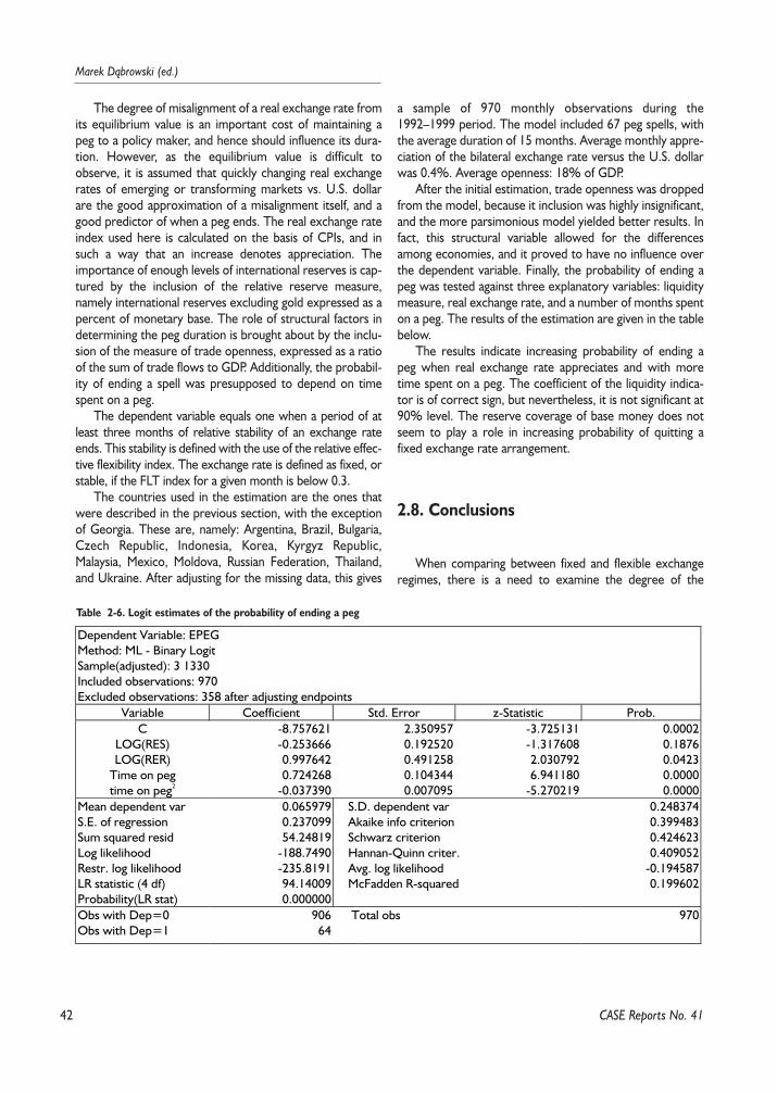
42
Marek D¹browski (ed.)
The degree of misalignment of a real exchange rate fromits equilibrium value is an important cost of maintaining apeg to a policy maker, and hence should influence its dura-tion. However, as the equilibrium value is difficult toobserve, it is assumed that quickly changing real exchangerates of emerging or transforming markets vs. U.S. dollarare the good approximation of a misalignment itself, and agood predictor of when a peg ends. The real exchange rateindex used here is calculated on the basis of CPIs, and insuch a way that an increase denotes appreciation. Theimportance of enough levels of international reserves is cap-tured by the inclusion of the relative reserve measure,namely international reserves excluding gold expressed as apercent of monetary base. The role of structural factors indetermining the peg duration is brought about by the inclu-sion of the measure of trade openness, expressed as a ratioof the sum of trade flows to GDP. Additionally, the probabil-ity of ending a spell was presupposed to depend on timespent on a peg.
The dependent variable equals one when a period of atleast three months of relative stability of an exchange rateends. This stability is defined with the use of the relative effec-tive flexibility index. The exchange rate is defined as fixed, orstable, if the FLT index for a given month is below 0.3.
The countries used in the estimation are the ones thatwere described in the previous section, with the exceptionof Georgia. These are, namely: Argentina, Brazil, Bulgaria,Czech Republic, Indonesia, Korea, Kyrgyz Republic,Malaysia, Mexico, Moldova, Russian Federation, Thailand,and Ukraine. After adjusting for the missing data, this gives
a sample of 970 monthly observations during the1992–1999 period. The model included 67 peg spells, withthe average duration of 15 months. Average monthly appre-ciation of the bilateral exchange rate versus the U.S. dollarwas 0.4%. Average openness: 18% of GDP.
After the initial estimation, trade openness was droppedfrom the model, because it inclusion was highly insignificant,and the more parsimonious model yielded better results. Infact, this structural variable allowed for the differencesamong economies, and it proved to have no influence overthe dependent variable. Finally, the probability of ending apeg was tested against three explanatory variables: liquiditymeasure, real exchange rate, and a number of months spenton a peg. The results of the estimation are given in the tablebelow.
The results indicate increasing probability of ending apeg when real exchange rate appreciates and with moretime spent on a peg. The coefficient of the liquidity indica-tor is of correct sign, but nevertheless, it is not significant at90% level. The reserve coverage of base money does notseem to play a role in increasing probability of quitting afixed exchange rate arrangement.
2.8. Conclusions
When comparing between fixed and flexible exchangeregimes, there is a need to examine the degree of the
CASE Reports No. 41
Table 2-6. Logit estimates of the probability of ending a peg
Dependent Variable: EPEGMethod: ML - Binary LogitSample(adjusted): 3 1330Included observations: 970Excluded observations: 358 after adjusting endpoints
Variable Coefficient Std. Error z-Statistic Prob.C -8.757621 2.350957 -3.725131 0.0002
LOG(RES) -0.253666 0.192520 -1.317608 0.1876LOG(RER) 0.997642 0.491258 2.030792 0.0423
Time on peg 0.724268 0.104344 6.941180 0.0000time on peg2 -0.037390 0.007095 -5.270219 0.0000
Mean dependent var 0.065979 S.D. dependent var 0.248374S.E. of regression 0.237099 Akaike info criterion 0.399483Sum squared resid 54.24819 Schwarz criterion 0.424623Log likelihood -188.7490 Hannan-Quinn criter. 0.409052Restr. log likelihood -235.8191 Avg. log likelihood -0.194587LR statistic (4 df) 94.14009 McFadden R-squared 0.199602Probability(LR stat) 0.000000Obs with Dep=0 906 Total obs 970Obs with Dep=1 64
43
Currency Crises in Emerging Markets – Selected Comparative ...
exchange rate flexibility empirically. The flexibility indexused here allowed to difference between the declared andpursued exchange rate regimes and set ground for deeperanalysis.
Case study approach allowed for a detailed analysis ofthe exchange rate regime changes in some emerging mar-kets. It is clear that the eruptions of the currency criseswere not caused by the fixed regime choices themselves,but rather by the inconsistent macroeconomic policieswithin this financial framework. If a fixed arrangement is tobe sustainable, not only monetary policy must be directedtowards supporting its parity, but also trade, regulatory andfiscal policies must be geared towards maintaining theexchange rate stability.
The results of the econometric estimation further sup-port this argument. They point on the importance of thereal exchange rate misalignment magnified by longer pegduration in explaining the probability that a fixed regimeends. However, smaller reserve coverage of the basemoney does not seem to influence the probability of endinga peg spell. This fact probably reflects the inter-country dif-ferences in levels of monetization, irrespective where cur-rency crises were happening.
It is difficult to recommend one particular regime for alldescribed economies. However, it seems that with increas-ing capital mobility, countries nowadays face the choice oftwo corner solutions of possible exchange rate regime. If aneconomy decides for a floating arrangement, its exchangerate should be really free to move in response to marketforces. The additional requirement for the floating exchangeregime to be effective is that the monetary policy mustestablish a credible alternative nominal anchor. Then if acountry opts for a rigid form of an exchange rate arrange-ment, this is for a currency board or a full dollarisation(euroisation), it should create sound and transparent insti-tutions, and rules guaranteeing that the commitment iscredible. Giving up monetary policy may be even a goodsolution for countries that need to stabilise their economiesand have very bad record of their economic policies.
Still, it should be remembered that a conventional pegarrangement is difficult to sustain for a longer term in highinflation countries, where the credibility of the monetaryauthority is not high, and where the financial system isunderdeveloped. The exchange rate anchor adopted wheneconomic conditions are favourable, but not supported bythe appropriate set of other policies, cannot last for long.And it is important that realignments of the pegs should beconsidered when it is not already too late, and that expan-sionary monetary policy is not in line with a currency peg fora longer period of time. In addition, this type of exchangerate regime may promote short-term foreign currency bor-rowing on a large scale, as happened in Asia.
CASE Reports No. 41
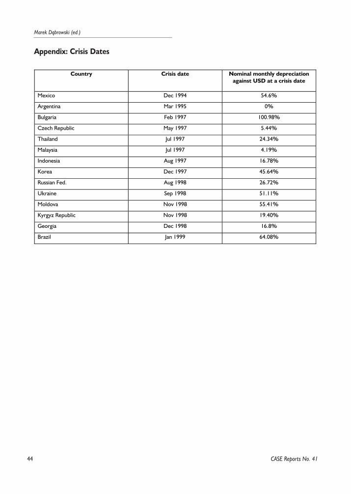
44
Marek D¹browski (ed.)
Appendix: Crisis Dates
CASE Reports No. 41
Country Crisis date Nominal monthly depreciationagainst USD at a crisis date
Mexico Dec 1994 54.6%
Argentina Mar 1995 0%
Bulgaria Feb 1997 100.98%
Czech Republic May 1997 5.44%
Thailand Jul 1997 24.34%
Malaysia Jul 1997 4.19%
Indonesia Aug 1997 16.78%
Korea Dec 1997 45.64%
Russian Fed. Aug 1998 26.72%
Ukraine Sep 1998 51.11%
Moldova Nov 1998 55.41%
Kyrgyz Republic Nov 1998 19.40%
Georgia Dec 1998 16.8%
Brazil Jan 1999 64.08%

45
Currency Crises in Emerging Markets – Selected Comparative ...
References
Aizenman J., R. Hausmann (2000). "Exchange RateRegimes and Financial Markets Imperfections". NBERWorking Paper No. 7738 (June).
Antczak R. (2000). "The Russian Crisis of 1998". Paperpresented at CASE conference on financial crises. Warsaw,December 21, 2000.
Baig, T., I. Goldfajn (2000). "The Russian Default and theContagion to Brazil". IMF Working Paper No. WP/00/160(October).
Balino T., A. Ubide (1999). "The Korean Financial Crisisof 1997 – A Strategy of Financial Sector Reform". IMFWorking Paper No. 99/28 (March).
Berg A. (1999). "The Asia Crisis: Causes, PolicyResponses, and Outcomes". IMF Working Paper No. 99/138(October).
Berg A., E. Borensztein (2000). "The Choice of ExchangeRate Regime and Monetary Target in Highly DollarizedEconomies". IMF Working Paper No. 00/29 (February).
Brudzyñski R., E. Mamirov (2000). "The Choice ofExchange Rate Regime for the Kyrgyz Republic: Official Dol-larization" (in Russian). CASE Studies and Analyses No. 216.
Céspedes L.F., R. Chang, A. Velasco (2000). "BalanceSheets and Exchange Rate Policy". NBER Working PaperNo. 7480 (August).
Chang R., A. Velasco (1999). "Liquidity Crises in Emerg-ing Markets: Theory and Policy". NBER Working Paper No.7272 (July).
Chang R., A. Velasco (1998). "The Asian Liquidity Crisis".NBER Working Paper No. 6796 (November).
Eichengreen B., R. Hausmann (1999). "Exchange Ratesand Financial Fragility". NBER Working Paper No. 7418(November).
Ganev G. (2001). "The Bulgarian Currency Crisis of1996–1997". Paper written within project on financial crisesat CASE, Warsaw.
Ganev G., M. Jarociñski, R. Lubenova, P. WoŸniak(2001). "Credibility of the Exchange Policy in TransitionCountries". CASE Reports No. 38.
Gulde am. M. (1999). "The Role of Currency Board inBulgaria's Stabilization". IMF Policy Discussion Paper No.PDP/99/3 (April).
Horváth J. (1999). "The May 1997 Currency Crisis inthe Czech Republic". Post-Communist Economies, Vol.11, No. 3.
IMF (2001). "Brazil: Selected Issues and StatisticalAppendix". IMF Staff Country Report No. 01/10 (January).
IMF (2000a). "Georgia: Recent Economic Developmentsand Selected Issues". Staff Country Report (April).
IMF (2000b). "Kyrgyz Republic. Selected Issues and Sta-tistical Appendix". IMF Staff Country Report (August).
IMF (2000c). "Repubilc of Moldova: Recent EconomicDevelopments". IMF Staff Country Report No. 88/110.
IMF (1999a)." Bulgaria: Recent Economic Developmentsand Statistical Appendix". Staff Country Report No. 99/26(April).
IMF (1999b). "Malaysia: Selected Issues". Staff CountryReport No. 99/86 (August).
IMF (1999c). "Russian Federation: Recent EconomicDevelopments". Staff Country Report No. 99/100 (Septem-ber).
IMF (1999d)." Ukraine: Recent Economic Develop-ments". IMF Staff Country Report No. 99/42 (May).
IMF (1998). "Czech Republic: Recent Economic Devel-opments and Statistical Appendix". Staff Country ReportNo. 98/37 (April).
IMF and WB (2001). "Armenia, Georgia, Kyrgyz Repub-lic, Moldova, and Tajikistan: External Debt and Fiscal Sus-tainability". Advance copy. IMF and WB: Washington.
Jakubiak M. (2000). "Currency Crisis in Argentina".Paper presented at CASE conference on financial crises.Warsaw, December 21, 2000.
Jakubiak M. (2000). "Indicators of Currency Crisis:Empirical Analysis of Some Emerging and TransitionEconomies". CASE Studies and Analyses No. 218.
Jarociñski M. (2000). "Moldova in 1995–1999: Macro-economic and Monetary Consequences of Fiscal Imbal-ances". CASE Studies and Analyses No. 205.
Kalter E., A. Ribas (1999). "The 1994 Mexican Econom-ic Crisis: The Role of Government Expenditure and RelativePrices". IMF Working Paper No. 99/160 (December).
Klein M., N. Marion (1997). "Explaining the Duration ofExchange Rate Pegs". Journal of Development Economics,Vol. 54, pp. 387–404.
Lane T., A. Ghosh, J. Haman, S. Philips, M. Schulze-Ghat-tas, T. Tsikata (1999). "IMF Supported Programs in Indone-sia, Korea and Thailand". A Preliminary Assesment. IMF:Washington.
Lubarova L., O. Petrushin, A. Radziwi³³ (2000). "IsMoldova Ready to Grow? Assessment of Post-Crisis Policies1999–2000". CASE Studies and Analyses No. 220.
Kovatchevska P. (2000). "The Banking and Currency Crisesin Bulgaria: 1996–1997". CASE Studies and Analyses Vol. 204.
Markiewicz M. (2000). "Financial Crisis in Ukraine".Paper presented at CASE conference on financial crises.Warsaw, December 21, 2000.
Mendoza E., M. Uribe (1999). "The Business Cycles ofBalance-of-Payment Crises: A Revision of Mundellan Frame-work". NBER Working Paper No. W7045 (March).
Mishkin F. (2001). "Financial Policies and the Preventionof Financial Crises in Emerging Market Countries". NBERWorking Paper No. 8087 (January).
Mishkin F. (1999). "International Experiences with Dif-ferent Monetary Policy Regimes. NBER Working Paper No.7044 (March).
CASE Reports No. 41
46
Marek D¹browski (ed.)
Mongardini J., J. Mueller (2000). "Ratchet Effects in Cur-rency Substitution: An Application to the Kyrgyz Republic".IMF Staff Papers Vol. 47, No. 2.
Mundell R. (1960). "The Monetary Dynamics of Interna-tional Adjustment Under Fixed and Flexible ExchangeRates". Quarterly Journal of Economics, No. 2, pp. 227–257.
Mussa M., P. Masson, A. Swoboda, E. Jadresic, P. Maoro,A. Berg (2000). "Exchange Rate Regimes in an IncreasinglyIntegrated World Economy". IMF: Washington.
Obsfeld M. (1997). "Open-Economy Macroeconomics,Developments in Theory and Policy". NBER Working PaperNo. 6319 (June).
Paczyñski W. (2000). "The Mexican Peso Crisis1994–1995". Paper presented at CASE conference on finan-cial crises. Warsaw, December 21, 2000.
Pitt A. (2001). "Sustaining Fixed Exchange Rates: AModel with Debt and Institutions". IMF Working Paper No.WP/01/27 (March).
Poirson H. (2001). "How Do Countries Choose TheirExchange Rate Regime?". IMF Working Paper No. WP/01/46(April).
Radziwi³³ A., O. Scerbatchi, C. Zaman (1999). "FinancialCrisis in Moldova – Causes and Consequences". CASE Stud-ies and Analyses Vol. 192.
Roubini N., P. Wachtel (1998). "Current Account Sus-tainability in Transition Economies". NBER Working PaperNo. 6468 (March).
Sasin M. (2001a). "The Indonesian Currency Crisis,1997–1998". Paper written for the June 2001 CASE confer-ence on currency crises.
Sasin M. (2001b). "The Malaysian Currency Crisis,1997–1998". Paper written for the June 2001 CASE confer-ence on currency crises.
Siwiñska J. (2000). "Currency Crises and Fiscal Imbal-ances – The Transition Countries Perspective". CASE Stud-ies and Analyses Vol. 219.
Szczurek M. (2001). "International Liquidity and theCosts of Currency Crises". Paper written for the June 2001CASE conference on currency crises.
CASE Reports No. 41
47
Currency Crises in Emerging Markets – Selected Comparative ...
CASE Reports No. 41
3.1. Introduction
Calls for higher foreign liquidity holding [Feldstein,1999; Mishkin, 1999; Radelet and Sachs, 1998] require aserious theoretical and empirical analysis of benefits andcosts of maintaining high liquidity. The paper aims at eval-uating the optimal level of foreign exchange reserves withrespect to currency crises in emerging markets. Simplepolicy optimisation model is presented, which is then eval-uated empirically.
The crises (including big crises) are nothing new [seeexcellent survey in Bordo and Schwartz, 1999, whichdescribes currency crises since 1830], but they appear toelude the attempts to model them. Many crises of the1930s, speculative attacks of the late Bretton-Woods eraand the ones troubling Latin American economies in 70sand 80s could well be explained by early, "first-generation"models [1] in which crisis erupts as a result of a macro-economic policy incompatible with fixed exchange rates.The catastrophes of the 1990s often require a differentapparatus. Thus appeared "second-generation" models inwhich rational government chooses (or not) to devalue, inan utility optimising process and in which rational agentstry to predict government choices [2]. Other models (gen-eration not yet given) started also to appear: liquiditymodels [e.g. Chang and Velasco, 1999], moral hazard[Dooley, 1997; Krugman, 1998; Corsetti, Pesenti andRoubini, 1999] and others. Second generation, as well aslater models often allow for analysing new features, crucialfor understanding the currency crises of the 1990s. Theyinclude contagion, multiple equilibria, self-fulfilling attacks,and crisis propagation.
As always, along formal models aiming at explanation ofwhat happened, post mortem accounts of the crises,together with policy advice were being published [3]. Thepolicy recommendations stated in these papers are surpris-
ingly similar. They can be summarised in the followingpoints:
– Fixed exchange rates are dangerous (country can haveonly two out of capital mobility, freedom of monetary poli-cy and fixed exchange rate),
– Banks should be very closely supervised, foreign par-ticipation in the sector would help,
– In the absence of international lender of the lastresort, and with a possibility of self-fulfilling attacks, interna-tional liquidity is the key to self protection.
The last point indeed seems to make perfect sense:even with less-than perfect macro policy, the governmentcould survive any speculative attack, provided it has enough"foreign exchange ammunition". What is more, if thereserves are high enough, the attack (bound to fail) willnever happen. The simple argument for higher reserves isnot obvious, however.
First, in monetary terms sterilised intervention (and for-eign exchange interventions are very often sterilised) shouldnot matter that much for the exchange rate. The mainproblem here is that sterilisation increases the potential forhot money outflow – "multiplies the enemy with the sameamount of ammunition" to stick with the military parable. Ifthe foreign exchange intervention is not sterilised, the econ-omy (and the banking sector in particular) must be able tosurvive a serious liquidity squeeze (which could have worseeffects than devaluation itself).
Second, in fixed exchange regime "sufficient liquidity" maymean foreign exchange reserves close to money supply. Anylevel of reserves smaller than this does not fully eliminate the"attack" equilibrium, as not only foreign investors, but also res-idents could choose to exchange domestic for foreign curren-cy. It may well be that relationship between foreign exchangereserves and probability of a crisis is not linear at all – it wouldbe plausible that a country with very high reserves would enjoyalmost zero probability of a speculative attack. Reserves evenmarginally smaller than that could warrant much higher risk.
Part III.International Liquidity, and the Cost of Currency CrisesMateusz Szczurek
[1] Including Krugman (1979), Flood and Garber (1984).[2] See e.g. Obstfeld (1994, 1996), Velasco (1996) Ozkan and Sutherland (1998), Drazen (1999).[3] Feldstein (1999), Mishkin (1999), Obstfeld (1998), Edwards (1999), Kamin (1999), Radelet and Sachs (1998) are just a few.
48
Marek D¹browski (ed.)
CASE Reports No. 41
Finally, liquidity is costly. Even if the government issuesinternational debt solely for the purpose of building up thewar chest of international reserves (with the annual cost ofthe spread over the US Treasuries) the gain in terms of liq-uidity will be limited because of the additional build-up ofobligations. If the proper measure of liquidity includes thelevel of short-term debt, borrowing short to build upreserves will make little sense. Still, provided the interna-tional reserves are built up with the long-term bonds, anincrease of international liquidity is feasible.
The problems indicated above should not lead to a con-clusion that reserves do not matter. Empirical studies sug-gest that there is significant evidence that international liq-uidity was a good predictor of the recent crises [4]. So far,however, there has been little research done to link theo-retical models with econometric research.
Thus, the following chapter tries to establish the theo-retical relationship between foreign exchange reserves andcurrency crises. Existing currency crisis models arereviewed, starting from Krugman (1979) "first generation"crisis model through several "second generation" optimisinggovernment models. New models dealing explicitly withinternational liquidity [like Chang and Velasco, 1999] arethen evaluated.
The paper will then include a short survey of empiricalstudy in which international liquidity plays a role.
After the review of the theoretical, as well as the empir-ical literature, a simple model of optimising government willbe presented. In the model, international reserves are theonly variable under the direct control of the policy-maker,which tries to minimise the probability of a currency crisis,having in mind the costs of foreign exchange reserves. Usingthe structure presented it is possible to estimate the implic-it reputation cost of the prospective currency crash to thepolicy-maker.
The final step was empirical testing of the model. Pooledlogit regression study was performed to check if differentmeasures of international liquidity help in surviving emergingmarket crises [5], and an attempt was made to approximatea reasonable amount of foreign exchange reserves in suchcountries. Developed markets currency crises rarely seemto be resulting from poor liquidity nowadays. Not only thelevel of international reserves they hold is usually higherthan in the emerging economies, but more importantly, thesolvency of industrialised countries' governments is never inquestion, therefore such countries enjoy easy access tointernational credit even in times of distress. Other equa-
tions of the model were also estimated, which allowed for anumerical estimation of reputation costs of the crisis toemerging economies' authorities.
The results confirm the appropriateness of the model'sfoundations. Almost all the parameters of the model (esti-mated over the sample of emerging market countries)behave as predicted by the theory. It allowed for estimationof the curve of reasonable holdings of the foreign exchangereserves. Assuming that a currency crisis costs only 1% ofthe GDP, the FX reserves should be 1.64 times higher thanthe foreign short-term debt (as reported by BIS). Given theconservative estimation of the crisis cost, this recommenda-tion clearly exceeds the IMF's prescription of reserve/shortterm debt ratio equal to one. Another result was the evalu-ation of the weight the governments/central banks of thecountries give to the risk of a currency crisis. The resultsshow that the policy makers of the emerging economies"value" a currency crisis at between 5 and 0.3% of the GDP.Surprisingly, the actual number does not seem to be corre-lated with the exchange rate arrangements.
3.2. Foreign Exchange Reserves in CrisisModels
3.2.1. A Survey of Literature
Beginning of the currency crisis literature is attributed toKrugman (1979) classic, later simplified and extended byFlood and Garber (1984) and surveyed in Agenor et al.(1992) [6]. So called first generation crisis models base onexhaustible resource literature originating in Hotelling(1931). The first generation crisis occurs as a result of anunreformable macroeconomic policy incompatible withfixed exchange rate. In Krugman's example the policy is theone of excessive fiscal deficits, monetised away. The inter-national reserves are quite central to the analysis: they takethe role of exhaustible resource in the equivalent model ofSalant and Henderson (1978). Incompatible macroeconom-ic policy causes gradual depletion of reserves. Fixedexchange regime can last only until foreign exchangereserves reach certain critical level. The model predicts,however, that the end comes earlier than that. Rationallythinking speculators attack and buy all remaining stock ofreserves as soon as the shadow price – the price which
[4] Radelet and Sachs (1998), Tornell (1999), Bussiere and Mulder (1999), IMF Early Warning System.[5] The literature on the subject is vast. Excellent survey of pre-1997 results is provided in Kaminsky, Lizondo and Reinhard (1997). New research
include: Tornell (1999), Rodric and Velasco (1999), Bussiere and Mulder (1999), Glick, Reuven and Rose (1999), Radelet and Sachs (1998), Chinn, Doo-ley and Shrestha (1999), and Tanner (1999). Still, each new crisis (and each new theory) provide some more scope for further research.
[6] Balance of payments models are older than that though. Mundell (1960) shows an example of a general equilibrium model in which abandon-ment of a peg depends on the level of international reserves.
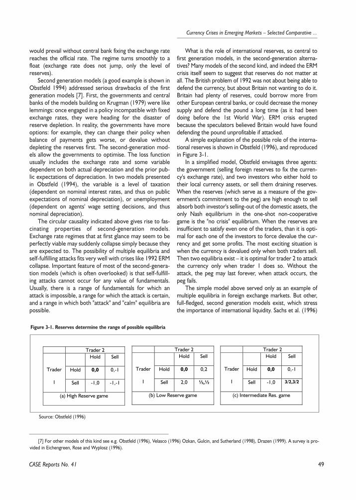
49
Currency Crises in Emerging Markets – Selected Comparative ...
CASE Reports No. 41
would prevail without central bank fixing the exchange ratereaches the official rate. The regime turns smoothly to afloat (exchange rate does not jump, only the level ofreserves).
Second generation models (a good example is shown inObstfeld 1994) addressed serious drawbacks of the firstgeneration models [7]. First, the governments and centralbanks of the models building on Krugman (1979) were likelemmings: once engaged in a policy incompatible with fixedexchange rates, they were heading for the disaster ofreserve depletion. In reality, the governments have moreoptions: for example, they can change their policy whenbalance of payments gets worse, or devalue withoutdepleting the reserves first. The second-generation mod-els allow the governments to optimise. The loss functionusually includes the exchange rate and some variabledependent on both actual depreciation and the prior pub-lic expectations of depreciation. In two models presentedin Obstfeld (1994), the variable is a level of taxation(dependent on nominal interest rates, and thus on publicexpectations of nominal depreciation), or unemployment(dependent on agents' wage setting decisions, and thusnominal depreciation).
The circular causality indicated above gives rise to fas-cinating properties of second-generation models.Exchange rate regimes that at first glance may seem to beperfectly viable may suddenly collapse simply because theyare expected to. The possibility of multiple equilibria andself-fulfilling attacks fits very well with crises like 1992 ERMcollapse. Important feature of most of the second-genera-tion models (which is often overlooked) is that self-fulfill-ing attacks cannot occur for any value of fundamentals.Usually, there is a range of fundamentals for which anattack is impossible, a range for which the attack is certain,and a range in which both "attack" and "calm" equilibria arepossible.
What is the role of international reserves, so central tofirst generation models, in the second-generation alterna-tives? Many models of the second kind, and indeed the ERMcrisis itself seem to suggest that reserves do not matter atall. The British problem of 1992 was not about being able todefend the currency, but about Britain not wanting to do it.Britain had plenty of reserves, could borrow more fromother European central banks, or could decrease the moneysupply and defend the pound a long time (as it had beendoing before the 1st World War). ERM crisis eruptedbecause the speculators believed Britain would have founddefending the pound unprofitable if attacked.
A simple explanation of the possible role of the interna-tional reserves is shown in Obstfeld (1996), and reproducedin Figure 3-1.
In a simplified model, Obstfeld envisages three agents:the government (selling foreign reserves to fix the curren-cy's exchange rate), and two investors who either hold totheir local currency assets, or sell them draining reserves.When the reserves (which serve as a measure of the gov-ernment's commitment to the peg) are high enough to sellabsorb both investor's selling-out of the domestic assets, theonly Nash equilibrium in the one-shot non-cooperativegame is the "no crisis" equilibrium. When the reserves areinsufficient to satisfy even one of the traders, than it is opti-mal for each one of the investors to force devalue the cur-rency and get some profits. The most exciting situation iswhen the currency is devalued only when both traders sell.Then two equilibria exist – it is optimal for trader 2 to attackthe currency only when trader 1 does so. Without theattack, the peg may last forever, when attack occurs, thepeg fails.
The simple model above served only as an example ofmultiple equilibria in foreign exchange markets. But other,full-fledged, second generation models exist, which stressthe importance of international liquidity. Sachs et al. (1996)
Figure 3-1. Reserves determine the range of possible equilibria
Source: Obstfeld (1996)
[7] For other models of this kind see e.g. Obstfeld (1996), Velasco (1996) Ozkan, Gulcin, and Sutherland (1998), Drazen (1999). A survey is pro-vided in Eichengreen, Rose and Wyplosz (1996).
Trader 2Hold Sell
Hold 0,0 0,-1Trader
1 Sell -1,0 -1,-1
(a) High Reserve game
Trader 2Hold Sell
Hold 0,0 0,2Trader
1 Sell 2,0 ½,½
(b) Low Reserve game
Trader 2Hold Sell
Hold 0,0 0,-1Trader
1 Sell -1,0 3/2,3/2
(c) Intermediate Res. game
50
Marek D¹browski (ed.)
CASE Reports No. 41
provides one example, in which the fundamental, whichgoverns the possibility of a successful attack, is the net levelof debt the government holds. Thus, sufficiently high level ofreserves (net of government debt) makes an attack impos-sible to succeed. Such a model seems to explain the stylisedfact of relative crisis immunity of highly liquid developingcountries.
Asymmetric information was quite early identified as animportant factor behind financial crises. Asian crisis provid-ed another example of how moral hazard (resulting fromimplicit government guarantees) can cause over-investment,excessive risk taking and a currency crisis. One of the advo-cates of the asymmetric information roots of many financialcrises was Mishkin (1998).
Right after the eruption of the Asian crisis, Paul Krugman(1998) suggested a moral hazard explanation to the crisis.His idea, in principle, was that implicit public guarantees forthe private enterprises generated excess demand for riskyinvestments. The firms (and their foreign creditors) wereconfident that if their project fails the government wouldbail them out. Of course, such logic cannot work in theeconomy-wide scale. When things went badly for East Asia(depreciation of the yen against the dollar, fall in semicon-ductor prices, etc.) too many projects started to fail. Thegovernment was not able to bail out everyone, short termforeign financing dried out and the currency plunged. Pesen-ti and Roubini (1999) present a formalised version of thismodel.
Dooley (1997) shows a similar story in his "insurancemodel." The latter model is especially interesting as it sug-gests that high international liquidity can actually cause adeterministic cycle resulting in a violent crisis. The mecha-nism suggested by Dooley works as follows.
Once (1) the government of a country has incentives tobail out domestic borrowers, (2) the government has a pos-itive net worth, and (3) capital account is sufficiently liber-alised, the crisis cycle starts. Domestic residents compete toborrow foreign money (knowing that the government willprovide free insurance, and will bail them out anyway if theyfail to pay – see 1 above), driving the domestic yieldupwards. Foreign creditors seeing that the government is(1) willing and (2) able to pay the insurance premium if theirborrowers fail to pay use (3) the liberalised capital accountto pump in the funds. As soon as the overall liabilities(including the implicit liabilities) of the government exceedavailable assets (these are not growing in line with liabilitiesbecause of moral-hazard induced excessive yield), the for-eign creditors rush to claim their insurance premium.Regardless of the exchange rate regime, resulting suddenoutflow of capital causes severe fiscal costs.
Recent years brought to the light several models dealingexplicitly with (lack of) international liquidity as a factorbehind foreign exchange crises. Typical model of this kind ispresented in Chang, Velasco (1999). The model is based on
the work on bank runs of Diamond and Dybvig (1983). Inthe models, the banking sector works as a term-structuretransformer, and as such has a structural asset-liability termmismatch. Because banks deal with many clients, they canuse law of large numbers to optimise their term structure,amount of reserves held, and long-term investments under-taken. The optimised (in terms of expected profit) amountof reserves, however, usually gives rise to a multiple equilib-rium solution. Either an outcome superior to the privatecompetitive (without bank inter-mediation) equilibrium pre-vails, or run on banks happens. Because the small liquidationvalue of the non-liquid assets, this outcome is usually worsethan the private competitive solution.
The translation of such a model of a bank run to theworld of foreign exchange crises is then quite straightfor-ward. If foreign depositors decide to run on the (insuffi-ciently liquid) banking sector, either banks fail (if the centralbank does nothing), or fixed exchange system collapses (ifthe central bank provides liquidity to the sector by printingmoney after using up insufficient foreign exchange reserves).The level of international liquidity is crucial, the more inter-national reserves the central bank has, the less severe bank-ing/currency crisis is. Floating exchange rate regime doesseem to ease some problems of insufficient liquidity, butonly if majority of debt in the economy is in local currency.The problem faced by most of the emerging markets, how-ever, is foreign debt denominated in foreign currency (also,foreign exchange crisis influences the quality of domestic-currency debt, as it can hit the value of collateral, see e.g.Mishkin, 1998).
The class of models does not only explain how runs oninsufficiently liquid banking sectors can translate into cur-rency crises. It also shows that the overall liquidity level heldby the sector may be optimal from expected return point ofview, but it may still give rise to a switch to a crisis equilibri-um. While it is quite easy to remain liquid, it is rational (cer-tainly for individual banks, but also often for the economy asa whole after taken into account the social cost of the sys-temic crisis) to have some maturity mismatch. Similar argu-ment applies to the term structure – high short-termindebtedness may be individually rational (although it can besocially inferior to long-term debt) – see Rodric and Velasco(1999).
Other models explicitly dealing with liquidity include:Goldfajn and Valdez (1997), Chang, Velasco (1998ab), andKrugman (1999).
3.2.2. A Survey of Empirical Results
The importance of the international liquidity in prevent-ing or easing the currency crises shown in the theoreticalmodels was also confirmed in many empirical studies. In anextensive research of 117 currency crashes Frankel and
51
Currency Crises in Emerging Markets – Selected Comparative ...
Rose (1996) concluded that variables important for predict-ing currency crises (defined as 25% depreciation of thelocal currency) include FDI/debt ratio, level of internationalreserves, high domestic credit growth, increase in worldinterest rates, real exchange rate overvaluation, and reces-sions. Current account and fiscal deficit were found to beinsignificant.
A study in a similar, univariate spirit was conductedrecently by Aziz, Caramazza and Salgado (2000). In thestudy based on 50 countries in a sample spanning from 1975to 1997 they found that out of the most of the 157 crisesrecorded were preceded by a fall in international liquidity(M2/international reserves).
Sachs, Tornell, and Velasco (1995) also show thatM2/international reserves coupled with weak fundamentalsrendered the countries vulnerable to contagion effects fol-lowing the Mexican crisis.
In another study, Tornell (1999) presents three determi-nants of the vulnerability of economies to the currencycrises: weakness of the banking sector, real appreciation ofthe local currency and international liquidity. Tornell foundthat some non-linear dependencies between the variables.For example, if international liquidity is high enough, thaneven significant real appreciation or banking sector fragilitydo not matter.
Bussiére and Mulder (1999) point to the importance ofinternational liquidity (defined as short term foreign debt toreserves ratio) in predicting the depth of a currency crisis.This variable, together with real appreciation of the localcurrency over the preceding four years, current accountdeficit and lack of an IMF support programme was able toexplain much of the depreciation of the emerging markets'currencies during the recent contagious crises. What ismore, multiplicative specification of the model (whereinternational liquidity dominates the overall vulnerabilityindex when it is very low or very high) seemed to performeven better.
Rodric and Velasco (1999) present yet another proofthat low international liquidity actually welcomes a curren-cy crisis (defined as a sharp reversal of capital flow) [8].Their probit analysis shows that short term debt/reservesratio (especially short term debt to foreign banks) signifi-cantly increases the probability of a crisis. Interestingly, thelevel of long-term and medium-term debt is significantlynegatively correlated with the probability of a crisis. Theexplanation for this could be that long-term debt is associ-ated with other, positive, country attributes (omitted from
the analysis). Rodric and Velasco also find out that short-term debt to international reserves ratio helps in explainingthe severity of the foreign exchange crises (measured as aGDP cost or depreciation).
The above survey of the literature touched upon animportant problem in measuring the crisis vulnerability –definitions of the crucial variables. The problem starts veryearly: how do we define a currency crisis? Table 3-1 sum-marises how different authors defined a currency crisis.
Similar "definitional" problem relates to the interna-tional liquidity. In a sense, the problem is deeper here, asit involves not only subjective view of what we call a crisis(as in the previous case), but also the economic theory.We can broadly define international liquidity as the abilityof a central bank / economy to survive a temporary capitalflow reversal without serious macroeconomic (e.g.exchange rate or GDP growth) consequences. Translatingsuch a definition into the world of available indicators isdifficult. One side of the equation (international assetsavailable on short notice) is quite easy to determine – in avast majority of cases it is defined as the stock of interna-tional reserves [9].
The problem starts with the definition of "hot" liabili-ties. How many obligations the central bank may be forcedto honour depend on many factors. For example, under afixed exchange rate regime the central bank should theo-retically be able to buy all the money stock for dollars (orother reserve currency) from the public. How much thecentral bank should actually be ready to buy out dependson e.g. the level of dollarisation of the economy. In coun-tries like Bosnia and Herzegovina, DM can easily be usedfor transactional purposes, thus in times of foreignexchange distress, the transactional demand for local cur-rency will be close to zero. Therefore in such country thecentral bank must be prepared to buy out the entiremoney stock from the public.
Weak banking sector enlarges the potential liability ofthe central bank (banking sector panic requires a boost inmoney supply, which may lead to depreciation). Similarly,the implicit guarantees towards the private corporatesector increase requirements for the overall liquidity ofthe government/central bank. Asian difficulties, modelledin Krugman (1999), and Dooley (1997) are a good exam-ple of this. Thus, while it seems plausible that sovereignshort-term debt should carry slightly bigger weight thanprivate sector liabilities, the latter should be far biggerthan zero. The private sector debt is likely to drain the
CASE Reports No. 41
[8] Radelet and Sachs (1998) reach similar conclusions in their study, which employs similar methodology.[9] Sometimes an international support may effectively increase the international liquidity (see the regression results in Bussiére and Mulder who
show that IMF support programmes reduce the vulnerability). On the other hand, the official foreign exchange reserves are sometimes more then theactual available assets. For example, central banks do not report their off-balance sheet obligations. Simple forward transactions (an obligation to e.g.sell foreign exchange in the future) are not represented in official reserves statistics. Central banks may also invest their foreign exchange in illiquid, orexcessively risky assets. Blejer and Schumacher (1998) advocate the use of Value-at-Risk approach to assess the central bank vulnerability. For somestatistics on discrepancy between official reserves and actually available assets see Aizenman and Marion (1999).
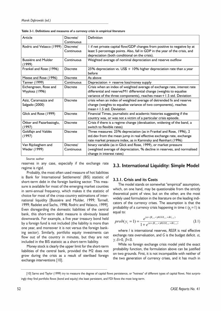
52
Marek D¹browski (ed.)
reserves in any case, especially if the exchange rateregime is rigid.
Probably, the most often used measure of hot liabilitiesis Bank for International Settlements' (BIS) statistic ofshort-term debt in the foreign banking sector. This mea-sure is available for most of the emerging market countiesin semi-annual frequency, which makes it the statistic ofchoice for most of the cross-country estimations of inter-national liquidity [Bussiére and Mulder, 1999; Tornell,1999; Radelet and Sachs, 1998; Rodric and Velasco, 1999].Even disregarding the domestic liabilities of the centralbank, this short-term debt measure is obviously biaseddownwards. For example, a five year treasury bond heldby a foreign fund is not included (the liability is more thanone year, and moreover it is not versus the foreign bank-ing sector). Similarly, portfolio equity investments canflow out of the country in minutes, but they are notincluded in the BIS statistic as a short-term liability.
Money stock is clearly the upper limit for the short-termliabilities of the central bank, provided the M2 does notgrow during the crisis as a result of sterilised foreignexchange interventions [10].
3.3. International Liquidity: Simple Model
3.3.1. Crisis and its CostsThe model stands on somewhat "empirical" assumption,
which, on one hand, may be questionable from the strictlytheoretical point of view, but on the other, are the mostwidely used formulation in the literature on the leading indi-cators of the currency crises. The assumption is that theprobability of a currency crisis happening in time t (yt=1) isequal to:
(3.1)
where l is international reserves, REER is real effectiveexchange rate overvaluation, and G is the budget deficit. α,γ, δ>0, β<0.
While no foreign exchange crisis model yield the exactprobability function, the formulation above can be justifiedon two grounds. First, it is not incompatible with neither ofthe two generation of currency crises, and it has much in
CASE Reports No. 41
Table 3-1. Definitions and measures of a currency crisis in empirical literature
Article Discrete/Continuous
Definition
Rodric and Velasco (1999) Discrete/Continuous
1 if net private capital flow/GDP changes from positive to negative by atleast 5 percentage points. Also, fall in GDP in the year of the crisis, anddepreciation (both conditional on the crisis).
Bussiére and Mulder(1999)
Continuous Weighted average of nominal depreciation and reserve outflow
Frankel and Rose (1996) Discrete 25% depreciation vs. US$ + 10% higher depreciation rate than a yearbefore
Meese and Rose (1996) Discrete As aboveTanner (1999) Continuous Depreciation + reserve loss/money supplyEichengreen, Rose andWyplosz (1996)
Discrete Crisis when an index of weighted average of exchange rate, interest ratedifferential and reserve/M1 differential change (weights to equalisevariance of the three components), reaches mean+1.5 std. Deviation
Aziz, Caramazza andSalgado (2000)
Discrete crisis when an index of weighted average of detrended fx and reservechange (weights to equalise variance of two components), reachesmean+1.5 std. Deviation
Glick and Rose (1999) Discrete Financial Times, journalistic and academic histories suggesting if thecountry was, or was not a victim of a particular crisis episode.
Ötker and Pazarbasioglu,(1997)
Discrete Crisis if there is a regime change (devaluation, widening of the band, aswitch to flexible rates)
Goldfajn and Valdés(1997)
Discrete Three measures: 25% depreciation (as in Frankel and Rose, 1996), 2std.dev from the mean jump in real effective exchange rate, exchangerate market pressure index, as in Kaminsky and Reinhart (1996)
Van Rijckeghem andWeder (1999)
Discrete/Continuous
binary variable (as in Glick and Rose, 1999), or market pressure(weighted average of depreciation, % decline in reserves, and normalisedchange in interest rates)
Source: author
[10] Sarno and Taylor (1999) try to measure the degree of capital flows persistence, or "hotness" of different types of capital flows. Not surpris-
ingly they find portfolio flows (bond and equity) the least persistent, and FDI flows the most long-term.
)(
)(
111
111
1)1(
−−−
−−−
+++
+++
+==
ttt
ttt
GREERl
GREERl
t eeyprob δγβα
δγβα
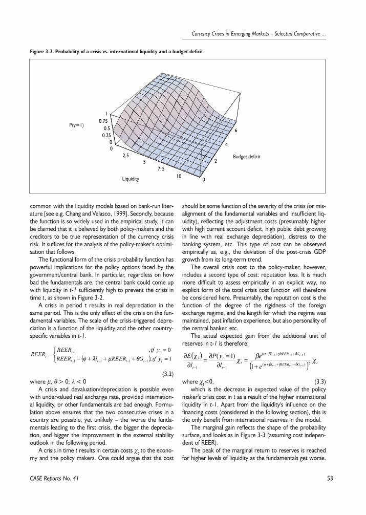
53
Currency Crises in Emerging Markets – Selected Comparative ...
common with the liquidity models based on bank-run liter-ature [see e.g. Chang and Velasco, 1999]. Secondly, becausethe function is so widely used in the empirical study, it canbe claimed that it is believed by both policy-makers and thecreditors to be true representation of the currency crisisrisk. It suffices for the analysis of the policy-maker's optimi-sation that follows.
The functional form of the crisis probability function haspowerful implications for the policy options faced by thegovernment/central bank. In particular, regardless on howbad the fundamentals are, the central bank could come upwith liquidity in t-1 sufficiently high to prevent the crisis intime t, as shown in Figure 3-2.
A crisis in period t results in real depreciation in thesame period. This is the only effect of the crisis on the fun-damental variables. The scale of the crisis-triggered depre-ciation is a function of the liquidity and the other country-specific variables in t-1.
(3.2)where µ, θ > 0; λ < 0
A crisis and devaluation/depreciation is possible evenwith undervalued real exchange rate, provided internation-al liquidity, or other fundamentals are bad enough. Formu-lation above ensures that the two consecutive crises in acountry are possible, yet unlikely – the worse the funda-mentals leading to the first crisis, the bigger the deprecia-tion, and bigger the improvement in the external stabilityoutlook in the following period.
A crisis in time t results in certain costs χt to the econo-my and the policy makers. One could argue that the cost
should be some function of the severity of the crisis (or mis-alignment of the fundamental variables and insufficient liq-uidity), reflecting the adjustment costs (presumably higherwith high current account deficit, high public debt growingin line with real exchange depreciation), distress to thebanking system, etc. This type of cost can be observedempirically as, e.g., the deviation of the post-crisis GDPgrowth from its long-term trend.
The overall crisis cost to the policy-maker, however,includes a second type of cost: reputation loss. It is muchmore difficult to assess empirically in an explicit way, noexplicit form of the total crisis cost function will thereforebe considered here. Presumably, the reputation cost is thefunction of the degree of the rigidness of the foreignexchange regime, and the length for which the regime wasmaintained, past inflation experience, but also personality ofthe central banker, etc.
The actual expected gain from the additional unit ofreserves in t-1 is therefore:
where χt<0, (3.3)which is the decrease in expected value of the policy
maker's crisis cost in t as a result of the higher internationalliquidity in t-1. Apart from the liquidity's influence on thefinancing costs (considered in the following section), this isthe only benefit from international reserves in the model.
The marginal gain reflects the shape of the probabilitysurface, and looks as in Figure 3-3 (assuming cost indepen-dent of REER).
The peak of the marginal return to reserves is reachedfor higher levels of liquidity as the fundamentals get worse.
CASE Reports No. 41
Figure 3-2. Probability of a crisis vs. international liquidity and a budget deficit
05
55
100
2
4
6
00.250.5
0.751
2.
7.
P(y=1)
Liquidity
Budget deficit
( )
=+++−=
=−−−−
−
1,0,
1111
1
ttttt
ttt yifGREERlREER
yifREERREER
θµλφ ( )( ) tGREERl
GREERl
tt
t
t
t
ttt
ttt
ee
lyP
lE χβχχ
δγβα
δγβα
2)(
)(
11 111
111
1)1(
−−−
−−−
+++
+++
−− +=
∂=∂=
∂∂
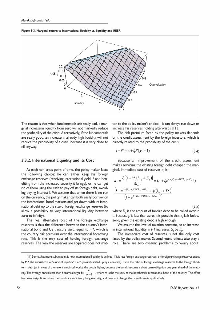
54
Marek D¹browski (ed.)
The reason is that when fundamentals are really bad, a mar-ginal increase in liquidity from zero will not markedly reducethe probability of the crisis. Alternatively, if the fundamentalsare really good, an increase in already high liquidity will notreduce the probability of a crisis, because it is very close tonil anyway.
3.3.2. International Liquidity and its Cost
At each non-crisis point of time, the policy maker facesthe following choice: he can either keep his foreignexchange reserves (receiving international yield i* and ben-efiting from the increased security it brings), or he can getrid of them using the cash to pay off its foreign debt, avoid-ing paying interest i. We assume that when there is no runon the currency, the policy maker can both easily borrow onthe international bond markets and get down with its inter-national debt up to the size of foreign exchange reserves (toallow a possibility to vary international liquidity betweenzero to infinity).
The real alternative cost of the foreign exchangereserves is thus the difference between the country's inter-national bond and US treasury yield, equal to i-i*, which isthe country risk premium over the international borrowingrate. This is the only cost of holding foreign exchangereserves. The way the reserves are acquired does not mat-
ter, to the policy maker's choice – it can always run down orincrease his reserves holding afterwards [11].
The risk premium faced by the policy makers dependson the credit assessment by the foreign investors, which isdirectly related to the probability of the crisis:
(3.4)
Because an improvement of the credit assessmentmakes servicing the existing foreign debt cheaper, the mar-ginal, immediate cost of reserves πt is:
(3.5)where Dt is the amount of foreign debt to be rolled over int. Because β is less than zero, it is possible that πt falls belowzero, given the existing debt is high enough.
We assume the level of taxation constant, so an increasein international liquidity in t-1 increases Gt by πt.
The immediate cost of reserves is not the only costfaced by the policy maker. Second round effects also play arole. There are two dynamic problems to worry about.
CASE Reports No. 41
[11] Somewhat more subtle point is how international liquidity is defined. If it is just foreign exchange reserves, or foreign exchange reserves scaled
by M2, the annual cost of "a unit of liquidity" is i-i* (possibly scaled up by a constant). If it is the ratio of foreign exchange reserves to the foreign short-
term debt (as in most of the recent empirical work), the cost is higher, because the bonds become a short term obligation one year ahead of the matu-
rity. The average annual cost then becomes larger by , where m is the maturity of the benchmark international bond of the country. The effect
becomes insignificant when the bonds are sufficiently long maturity, and does not change the overall results qualitatively.
Figure 3-3. Marginal return to international liquidity vs. liquidity and REER
0
0.2
0.4
0.6
0.8
1
00.050.1
0.150.2
US$ c
0
2
4
6
Liquidity
Overvaluation
1−mm
)1(* =+=− tyPii ξε
( )( )[ ]
( )[ ]( )2GREERl
t1tGREERl
GREERl
1t
t1tt
1t1t1t
1t1t1t
1t1t1t
e1Dle1
el
Dlii
−−−
−−−
−−−
+++−
+++
+++
−
−
++++
+=∂
+−∂=
δγβα
δγβα
δγβα
β
ξεπ )(*
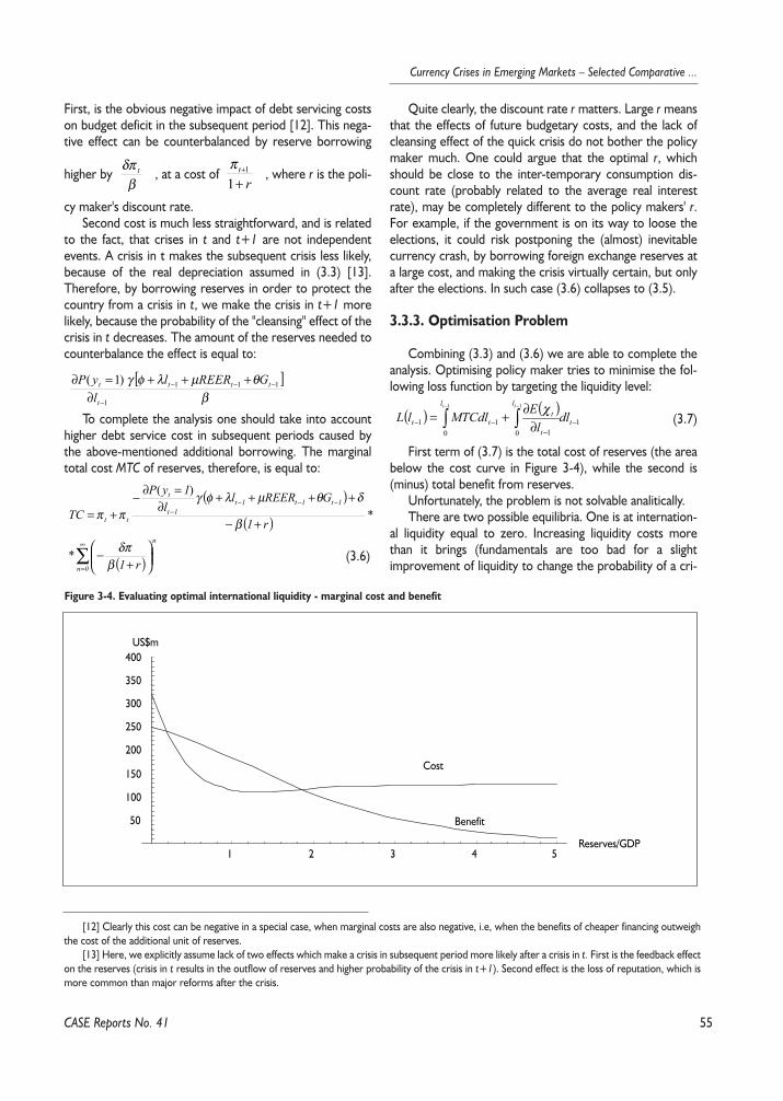
55
Currency Crises in Emerging Markets – Selected Comparative ...
First, is the obvious negative impact of debt servicing costson budget deficit in the subsequent period [12]. This nega-tive effect can be counterbalanced by reserve borrowing
higher by , at a cost of , where r is the poli-
cy maker's discount rate.Second cost is much less straightforward, and is related
to the fact, that crises in t and t+1 are not independentevents. A crisis in t makes the subsequent crisis less likely,because of the real depreciation assumed in (3.3) [13].Therefore, by borrowing reserves in order to protect thecountry from a crisis in t, we make the crisis in t+1 morelikely, because the probability of the "cleansing" effect of thecrisis in t decreases. The amount of the reserves needed tocounterbalance the effect is equal to:
To complete the analysis one should take into accounthigher debt service cost in subsequent periods caused bythe above-mentioned additional borrowing. The marginaltotal cost MTC of reserves, therefore, is equal to:
Quite clearly, the discount rate r matters. Large r meansthat the effects of future budgetary costs, and the lack ofcleansing effect of the quick crisis do not bother the policymaker much. One could argue that the optimal r, whichshould be close to the inter-temporary consumption dis-count rate (probably related to the average real interestrate), may be completely different to the policy makers' r.For example, if the government is on its way to loose theelections, it could risk postponing the (almost) inevitablecurrency crash, by borrowing foreign exchange reserves ata large cost, and making the crisis virtually certain, but onlyafter the elections. In such case (3.6) collapses to (3.5).
3.3.3. Optimisation Problem
Combining (3.3) and (3.6) we are able to complete theanalysis. Optimising policy maker tries to minimise the fol-lowing loss function by targeting the liquidity level:
(3.7)
First term of (3.7) is the total cost of reserves (the areabelow the cost curve in Figure 3-4), while the second is(minus) total benefit from reserves.
Unfortunately, the problem is not solvable analitically. There are two possible equilibria. One is at internation-
al liquidity equal to zero. Increasing liquidity costs morethan it brings (fundamentals are too bad for a slightimprovement of liquidity to change the probability of a cri-
CASE Reports No. 41
βδπ t
rt
++
11π
[12] Clearly this cost can be negative in a special case, when marginal costs are also negative, i.e, when the benefits of cheaper financing outweighthe cost of the additional unit of reserves.
[13] Here, we explicitly assume lack of two effects which make a crisis in subsequent period more likely after a crisis in t. First is the feedback effecton the reserves (crisis in t results in the outflow of reserves and higher probability of the crisis in t+1). Second effect is the loss of reputation, which ismore common than major reforms after the crisis.
[ ]β
θµλφγ 111
1
)1( −−−
−
+++∂
=∂ ttt
t
t GREERllyP
( )( )
( )∑∞
=
−−−−
+
−
+−
++++∂
=∂−+=
0n
n
1t1t1t1t
t
tt
r1
r1
GREERll
1yP
TC
βδπ
β
δθµλφγππ
*
*
)(
(3.6)
( ) ( )1
0 11
01
11
−−
−− ∫∫−−
∂∂+= t
l
t
tt
l
t dllEdlMTClL
tt χ
Figure 3-4. Evaluating optimal international liquidity - marginal cost and benefit
1 2 3 4 5Reserves/GDP
50
100
150
200
250
300
350
400US$m
Cost
Benefit

56
Marek D¹browski (ed.)
sis much). The second equilibrium is in the point wheredownward sloping marginal benefit and marginal cost curvescross. The second equilibrium is a global minimum only ifL(lt-1)<0. In the example above, it is clearly the optimal levelof liquidity: the total gain (which is the surface below themarginal benefit curve) exceeds the total cost.
The model has several advantages:1. It takes into account not only the obvious costs of liq-
uidity, but also the dynamic effects – the costs of postponingthe crisis.
2. It is relatively straightforward to estimate. The bene-fit function (logit analysis of the reserves' impact on theprobability of the crisis) is deeply rooted in the existing lit-erature on leading crisis indicators. Similarly, data for thedepth-of-crisis function, and interest rate premium relation-ship is widely available for a wide range of countries.
3. The model allows for an estimation of the reputationcost of the foreign exchange crisis (which is the only missingdata in the whole structure).
3.4. Empirical Application
The above model was used for two applications. First,we tried to estimate what is the optimal (safe, and reason-ably cheap – "best value for money") holding of internation-al liquidity. This requires certain assumption regarding theperceived cost of the currency crisis.
Second application involve finding out what is the per-ceived cost of the currency crisis to the policy-maker. Byassuming the countries analysed hold optimal (from thepoint of view of the policy maker) international liquidity, weare able to estimate "how much the crisis is feared", or thetotal cost the currency crisis (including the reputation cost),as viewed by the policymaker.
3.4.1. Data
The macro data for the empirical section comes mostlyfrom the IMF IFS CD-ROM. The variables used were:
Y, crisis dummy, calculated as in Eichengreen and Rose(1997). Y equals to one when weighted average of nominaldepreciation versus US$ and foreign exchange reserve lossexceeds 1.5 times standard deviation of the pooledexchange market pressure index.
REER, a measure of exchange rate overvaluation. It iscalculated as a percentage deviation from the long-term(1980–2000, or shorter when early real exchange rate datanot available) quarterly trend. Positive number meansappreciated real exchange rate.
LLBIS, a measure of international liquidity, calculated as aratio of foreign exchange reserves to foreign bank debt
maturing within one year (taken from BIS/OECD/WB/IMFdatabase).
G, budget balance as a percentage of GDP.SPREAD, benchmark bond spread over US treasury of
the same maturity. This variable was taken from ING Bar-ings' Emerging Markets Weekly Report tables.
The participation of a particular country in the global finan-cial markets was the main factor in the sample selectionprocess. Developed countries were skipped from the sample,and only emerging market countries dollar-denominatedbonds of which were quoted at some stage in the 1990s wereconsidered. The list of the countries in the sample is in theAppendix.
Two assumptions should be made for the estimation:first, the policy maker's discount rate r was set to 10% (theresults were not very responsive to the changes in this vari-able), and the "reasonable" cost of the currency crisis. Thelatter was much more difficult to choose, as indicated in theCrisis and its cost section above. We avoided the problem bypresenting the whole curve of optimal liquidity holding,dependent on the estimation of the prospective crisis cost.
3.4.2. The Results
The results of Equation (3.1) estimation are shown inTable 3-2.
All the parameters have right signs, but the significanceof the budget balance in influencing the probability of thecrisis is dubious. This allows us to drop the budget balancefrom the crisis probability equation, but also, we can ignorethe first of the dynamic effects from the total cost equation(the impact of the debt servicing costs on the subsequentbudget deficits).
International liquidity is the most significant variable inthe model. The model suggests that a country with foreignexchange reserves at 30% of the short term debt, and 30%overvalued real exchange rate has over 42% chance ofexperiencing a currency crisis.
Next step is estimating the scope of depreciation in caseof the crisis, conditional on the fundamental variables. Theresults of the OLS estimation are given in Table 3-3.
Again, all the parameters have correct signs, apart fromthe budget surplus variable, which is also not significant.
The final step is evaluating how sovereign spreads dependon the fundamentals and international liquidity. For this pur-pose MODEL variable was created from the fitted values ofthe crisis probability equation. The results are again consistentwith the theoretical model; higher fitted probability of the cri-sis leads to higher spreads over US Treasuries well ahead (oneyear) of the prospective crisis (Table 3-4).
The overall results are satisfying, i.e. consistent with themodel priors. They prove that international liquidity doesmatter very much in averting currency crises. The higher
CASE Reports No. 41
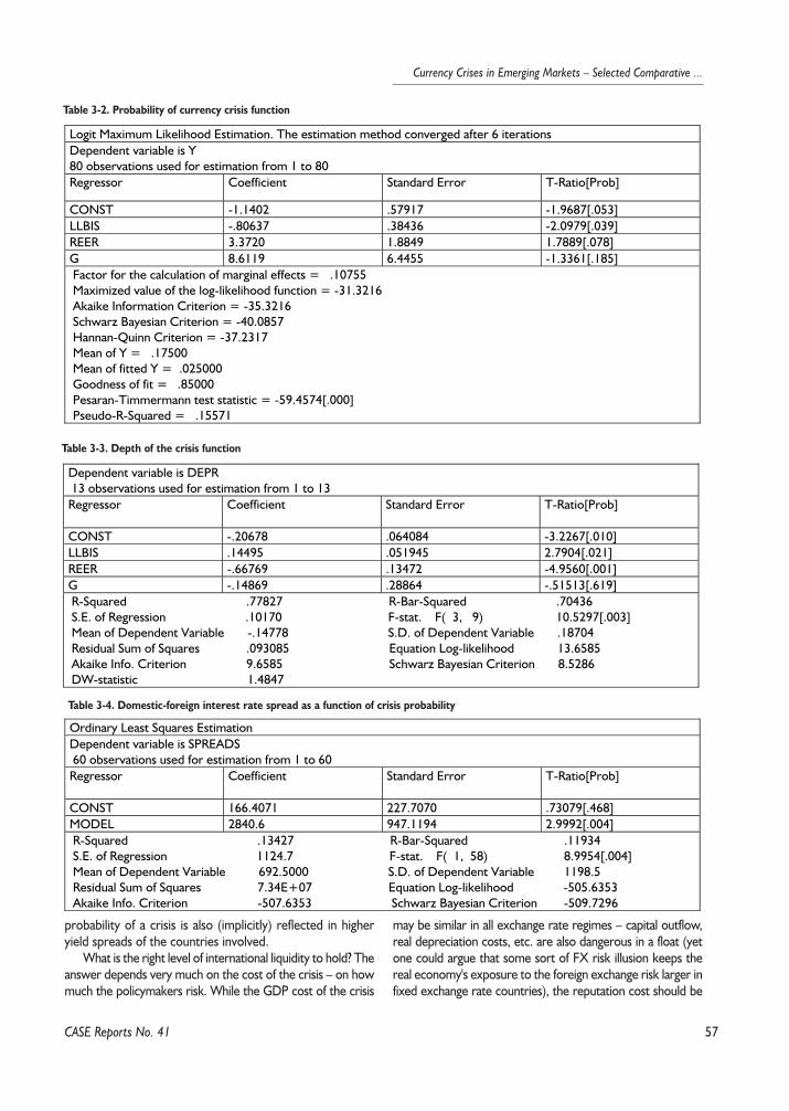
57
Currency Crises in Emerging Markets – Selected Comparative ...
probability of a crisis is also (implicitly) reflected in higheryield spreads of the countries involved.
What is the right level of international liquidity to hold? Theanswer depends very much on the cost of the crisis – on howmuch the policymakers risk. While the GDP cost of the crisis
may be similar in all exchange rate regimes – capital outflow,real depreciation costs, etc. are also dangerous in a float (yetone could argue that some sort of FX risk illusion keeps thereal economy's exposure to the foreign exchange risk larger infixed exchange rate countries), the reputation cost should be
CASE Reports No. 41
Table 3-2. Probability of currency crisis function
Logit Maximum Likelihood Estimation. The estimation method converged after 6 iterationsDependent variable is Y80 observations used for estimation from 1 to 80Regressor Coefficient Standard Error T-Ratio[Prob]
CONST -1.1402 .57917 -1.9687[.053]LLBIS -.80637 .38436 -2.0979[.039]REER 3.3720 1.8849 1.7889[.078]G 8.6119 6.4455 -1.3361[.185] Factor for the calculation of marginal effects = .10755 Maximized value of the log-likelihood function = -31.3216 Akaike Information Criterion = -35.3216 Schwarz Bayesian Criterion = -40.0857 Hannan-Quinn Criterion = -37.2317 Mean of Y = .17500 Mean of fitted Y = .025000 Goodness of fit = .85000 Pesaran-Timmermann test statistic = -59.4574[.000] Pseudo-R-Squared = .15571
Table 3-3. Depth of the crisis function
Dependent variable is DEPR 13 observations used for estimation from 1 to 13Regressor Coefficient Standard Error T-Ratio[Prob]
CONST -.20678 .064084 -3.2267[.010]LLBIS .14495 .051945 2.7904[.021]REER -.66769 .13472 -4.9560[.001]G -.14869 .28864 -.51513[.619] R-Squared .77827 R-Bar-Squared .70436 S.E. of Regression .10170 F-stat. F( 3, 9) 10.5297[.003] Mean of Dependent Variable -.14778 S.D. of Dependent Variable .18704 Residual Sum of Squares .093085 Equation Log-likelihood 13.6585 Akaike Info. Criterion 9.6585 Schwarz Bayesian Criterion 8.5286 DW-statistic 1.4847
Table 3-4. Domestic-foreign interest rate spread as a function of crisis probability
Ordinary Least Squares EstimationDependent variable is SPREADS 60 observations used for estimation from 1 to 60Regressor Coefficient Standard Error T-Ratio[Prob]
CONST 166.4071 227.7070 .73079[.468]MODEL 2840.6 947.1194 2.9992[.004] R-Squared .13427 R-Bar-Squared .11934 S.E. of Regression 1124.7 F-stat. F( 1, 58) 8.9954[.004] Mean of Dependent Variable 692.5000 S.D. of Dependent Variable 1198.5 Residual Sum of Squares 7.34E+07 Equation Log-likelihood -505.6353 Akaike Info. Criterion -507.6353 Schwarz Bayesian Criterion -509.7296

58
Marek D¹browski (ed.)
different. In the extreme float case, the central bank ignoresthe foreign exchange fluctuations, however rapid and largethey are, the reputation cost should thus be set to zero.Another complication arises due to the fact that the govern-ment's loss function is something completely different to the"economy's loss function". One could argue that what reallymatters in influencing the policymakers' liquidity preferencesare expected fiscal and quasi-fiscal costs of a currency crisis.
Surprisingly, the results of the next section do not sup-port expectations of the strong influence of currency regimeon the policymakers' aversion to the currency crises.
The results for the average (from the pool) country areshown in Figure 6. Vertical scale represents optimal liquidi-ty (as a reserves/short-term debt ratio) corresponding tothe assumed cost of the currency crisis (as a percentage ofGDP).
The results indicate that the IMF's recommendation ofkeeping foreign exchange reserves stock equal to the short-
term foreign debt is insufficient. Assuming the cost of thecrisis at just 1% of GDP, optimal international liquidity is 1.6times the short term foreign debt. If we believe the crisesare more costly than 1% of GDP, the reserves held be amultiple of the short-term foreign debt. It is important tostress that this prescription is applicable to the averagecountry from the sample, and may be sub-optimal for someof the analysed economies (which, for example, suffer fromexcessively high budget deficit, or exchange rate overvalua-tion).
3.4.3. How Much the Policy Makers Fear the Crisis?
The final empirical application of the model involves find-ing the cost of the crisis as seen (or expected) by the poli-cymaker. Assuming that the amount of international liquidi-ty held by the central banks is rational (in the model sense),
we can find out how much the policymakers fear the cur-rency crisis. The process involves finding out the value of χ(implicit estimation of crisis cost by the policymaker) forwhich marginal cost curve of the liquidity crosses marginalbenefit curve of the liquidity at the level of actually heldinternational reserves.
In the following analysis it sometimes happens that thecost curve has such a shape that it is impossible to find a χ,which would minimise the loss function at the desired levelof the international liquidity. In such cases to gain someinsight of the possible range of reputation cost χ, weassumed the largest χ for which the total benefit exceedstotal cost (both integrated between 0 and the actual inter-national liquidity held).
Table 3-5 shows the summary of the results, cost of thecurrency crises expected by the governments and centralbanks of the countries listed, as of end-99. Figure 3-6 showsgraphs of the 4Q99 liquidity's marginal cost and benefitscurves of the countries in the sample, as well as implicitexpected crisis cost – χ (in US$m).
The results show quite a wide disparity of implicit cur-rency crisis cost to the policy makers. Discarding the
Moldova's outlier (which, most probably results fromextremely low amount of short term BIS reported debt),the implicit cost estimation by the policymakers varies from5% of GDP (Malaysia) down to 0.3% (Dominican Republic).The results seem to have little to do with the exchange ratearrangements, which is somewhat disturbing: apart fromMalaysia, the first nine countries on the list have a floating ormanaged floating exchange rate.
CASE Reports No. 41
Figure 3-5. Optimal liquidity holding versus cost of the crisis
2 4 6 8 10
% GDP
1
2
3
4
5LLBIS
Table 3-5. Crisis cost to the policy maker, as of end-99
Country % of GDP US$mMOLDOVA 43.1% 500MALAYSIA 12.1% 9500CZECH REPUBLIC 5.0% 2650POLAND 3.3% 5220CHILE 2.7% 1800SLOVAK REPUBLIC 2.1% 420KOREA 2.0% 7950PHILIPPINES 1.8% 1370SOUTH AFRICA 1.5% 2000RUSSIA 1.4% 2650ARGENTINA 1.3% 3730COSTA RICA 1.2% 175ECUADOR 0.9% 180CHINA,P.R.: MAINLAND 0.9% 8600COLOMBIA 0.8% 710BRAZIL 0.8% 4150ROMANIA 0.4% 150PAKISTAN 0.4% 250DOMINICAN REPUBLIC 0.3% 50

Figure 3.6. Marginal liquidity cost and benefit curves in emerging markets
Argentina χ= 3730
1 2 3 4 5LLBIS
100
200
300
400
500
600
US$m
Brazil, χ=4150
2 4 6 8Reserves LLBIS
200
400
600
800
1000US$m
Chile, χ= 1800
1 2 3 4 5LLBIS
100
200
300
400
500
600
US$m
China (Mainland), χ= 8600
2 4 6 8LLBIS
-4000
-2000
2000
4000
6000
US$m
Colombia, χ= 710
2 4 6 8LLBIS
50
100
150
200
US$m
Costa Rica, χ= 175
2 4 6 8LLBIS
5
10
15
20
25
30
US$m
Czech Republic, χ= 2650
2 4 6 8LLBIS
25
50
75
100
125
150
175
US$m
Dominican Republic, χ= 50
2 4 6 8LLBIS
2
4
6
8
10
12
14
US$mEcuador, χ= 180
2 4 6 8LLBIS
5
10
15
20
25
30
US$m
Korea (South), χ= 7950
2 4 6 8LLBIS
200
400
600
800
1000
1200
1400
US$m
Malaysia, χ= 9500
2 4 6 8LLBIS
200
400
600
800
1000
1200
1400
US$m
Moldova, χ= 500
2 4 6 8LLBIS
1
2
3
4
5
US$mPakistan, χ= 250
2 4 6 8LLBIS
10
20
30
40
50
US$mPhilippines, χ= 1370
2 4 6 8LLBIS
50
100
150
200
250
US$m
Poland, χ= 5220
2 4 6 8LLBIS
50
100
150
200
US$m
Romania, χ= 150
2 4 6 8LLBIS
10
20
30
40
50
60
US$mRussia, χ= 2650
2 4 6 8LLBIS
50
100
150
200
250
US$m
Slovak Republic, χ= 420
2 4 6 8LLBIS
10
20
30
40
50
60
70
US$mSouth Africa, χ= 2000
1 2 3 4 5LLBIS
50
100
150
200
250
300
US$m
Sample mean, χ= 3200
2 4 6 8LLBIS
50
100
150
200
250
300
US$m
60
Marek D¹browski (ed.)
3.5. Conclusions
The paper presents review of the literature on the influ-ence of international liquidity on the incidence of currencycrises. It then presents a model of optimal liquidity holdingby the policy maker, in which optimal liquidity held dependson the fundamentals, international borrowing costs, and thepotential cost of the crisis to the policy maker.
The model presented in the paper appears to be apromising way to deal with costs and benefits of interna-tional liquidity. Almost all the parameters of the model (esti-mated over the sample of emerging market countries)behave as predicted by the theory. It allowed for estimationof the curve reasonable holdings of the foreign exchangereserves. Assuming that a currency crisis costs only 1% ofthe GDP, the FX reserves should be 1.64 times higher thanthe foreign short-term debt (as reported by BIS). Given theconservative estimation of the crisis cost, this recommenda-tion clearly exceeds the IMF's prescription of reserve/shortterm debt ratio equal to one.
Another set of results received thanks to the model wasthe weight the governments/central banks attach to the riskof a currency crisis. We found out that the policymakers ofthe countries analysed, behave, as if they predicted theprospective crisis would cost the budget between 5 and0.3% of the GDP. This result includes not only explicit bud-getary costs of the currency crisis, but also the reputationloss of the central bank, political losses of the governmentetc. To our knowledge it is the first estimation of this kind.Surprisingly, the actual number does not seem to be corre-lated with the exchange rate arrangements.
In case of some policy-makers the assumption of ratio-nality (in the model sense) does not seem to hold. Given themodel's specifications, some international liquidity holdingsare too small to find any crisis cost value, which would makethem optimal.
The paper leaves some scope for further research. Mainissues worth addressing are:
– The simplicity of the foreign financing cost function;– Enlarging the data sample. It was limited to the IMF IFS
data in the paper, which reduced the sample to 24 in someequations.
– Dealing with continuous, instead of binary, definitionsof a currency crisis.
Appendix
Countries in the data sample:
CASE Reports No. 41
ARGENTINABRAZILCHILECHINA,P.R.: MAINLANDCHINA,P.R.:HONG KONGCOLOMBIACOSTA RICACROATIACZECH REPUBLICDOMINICAN REPUBLICECUADORHUNGARYINDIAINDONESIAKAZAKHSTANKOREALEBANONMALAYSIAMEXICOMOLDOVAPAKISTANPANAMAPHILIPPINESPOLANDROMANIARUSSIASLOVAK REPUBLICSLOVENIASOUTH AFRICATHAILANDTURKEYURUGUAYVENEZUELA

61
Currency Crises in Emerging Markets – Selected Comparative ...
References
Agenor P., J. Aizenman (1997). "Contagion and Volatilitywith Imperfect Credit Markets". NBER WP No. 6080.
Agénor P-R, J.S. Bhandari, R.P. Flood (1992). "SpeculativeAttacks and Models of Balance of Payments Crises". NBERWP No. 3919.
Aizenman J., N. Marion (1999). "Reserve Uncertaintyand the Supply of International Credit". NBER WorkingPaper No. 7202.
Eichengreen B., A.K. Rose, Ch. Wyplosz (1996). "Conta-gious Currency Crises: First Tests". Scandinavian Journal ofEconomics, Vol. 98, No. 4, pp. 463–484.
Bacchetta P., E. van Wincoop (1998). "Capital Flows toEmerging Markets: Liberalisation, Overshooting, andVolatility". NBER WP No. 6530.
Baig T., I. Goldfajn (1998). "Financial Market Contagionin the Asian Crisis". IMF WP No. 98/155.
Blejer M.I., L. Schumacher (1998). "Central Bank Vul-nerability and the Credibility of Commitments: A Value-at-Risk Approach to Currency Crises". IMF WP No. 98/65.
B³aszkiewicz M., W. Paczyñski (2001). "The Economicand Social Consequences of Financial Crises". May 9,unpublished (Warsaw, CASE foundation).
Bordo M. D., A.J. Schwartz (1999). "Under What Cir-cumstances, Past and Present, Have International Rescuesof Countries in Financial Distress Been Successful?". Journalof International Money and Finance 18, pp. 683–708.
Bussiere M., Ch. Mulder (1999). "External Vulnerabilityin Emerging Market Economies: How High Liquidity CanOffset the Weak Fundamentals and the Effect of Conta-gion". IMF WP No. 99/88.
Calvo G.A., E.G. Mendoza (1999). "Rational Contagionand the Globalisation of the Securities Markets". NBER WPNo. 7153.
Chang R., A. Velasco (1999). "Liquidity Crises in Emerg-ing Markets: Theory and Policy". NBER WP No. 7272.
Chinn M.D., M.P. Dooley, S. Shrestha (1999). "LatinAmerica and East Asia crises in the context of an insurancemodel of currency crises". Journal of International Moneyand Finance 18, pp. 659–681.
Diamond D., P. Dybvig (1983). "Bank Runs, DepositInsurance, and Liquidity". Journal of Political Economy 91,pp. 401–419.
Dooley M.P. (1997). "A Model of Crises in EmergingMarkets". NBER WP No. 6300.
Drazen A. (1999). "Political Contagion in CurrencyCrises". NBER Working Paper No. 7202.
Edwards S. (1999). "Crisis Prevention: Lessons fromMexico and East Asia". NBER Working Paper No. 7233.
Feldstein M. (1999). "Self-Protection for Emerging Mar-ket Economies". NBER WP No. 6907.
Flood R., P. Garber (1984). "Collapsing Exchange RateRegimes: Some Linear Examples". Journal of InternationalEconomics 17, pp. 1–13.
Frankel J., A.K. Rose (1996). "Currency Crashes inEmerging Markets: An Empirical Treatment". Journal ofInternational Economics 41, pp 351–368.
Frobes K., R. Rigobon (1999). "No Contagion onlyInterdependence: Measuring Stock Market Co-move-ments". NBER WP No. 7267.
Frydl E. (1999). "The Length and Cost of BankingCrises". IMF WP No. 99/30.
Glick R., A.K. Rose (1999). "Contagion and trade: Whyare currency crises regional?". Journal of InternationalMoney and Finance 18, pp. 603–617.
Hotelling H. (1931). "The Economics of ExhaustibleResources." Journal of Political Economy, 39, pp. 137–25.
Kamin S.B. (1999). "The current international financialcrisis: how much is new?". Journal of International Moneyand Finance 18, pp. 501–514.
Kaminsky G., S. Lizondo, C.M. Reinhard (1997). "Lead-ing Indicators of Currency Crises". IMF WP No. 97/79.
Kaminsky G.L., S.L. Schmukler (1999). "What triggersmarket jitters? A chronicle of the Asian crisis". Journal ofInternational Money and Finance 18, pp. 537–560.
Kim W., S. Wei (1999). "Foreign Portfolio InvestorsBefore and During a Crisis". NBER WP No. 6968.
Krugman P. (1979). "A model of balance of paymentscrises". Journal of Money, Credit, and Banking 11, pp.311–325.
Krugman P. (1997). "Currency Crises". Mimeo (Cam-bridge, Massachusetts: MIT), http://web.mit.edu/krug-man/www/crises, (accessed on 2/12/2000).
Krugman P. (1999). "Analytical Afterthoughts on theAsian Crisis". Mimeo (Cambridge, Massachusetts: MIT),http://web.mit.edu/krugman/www/minicris.htm, (accessedon 2/12/2000).
Masson P. (1999). "Contagion: macroeconomic modelswith multiple equilibria". Journal of International Money andFinance 18, pp. 587–602.
Mendoza E.G., M. Uribe (1999). "The Business Cycles ofBalance-of-Payments crises: A Revision of a MundellianFramework". NBER WP No. 7045.
Mishkin F.S. (1998). "International Capital Movements,Financial Volatility and Financial Instability". NBER WPNo. 6390.
Mishkin F. (1999). "Lessons from the Asian Crisis". Jour-nal of International Money and Finance 18, pp. 709–723.
Mizen P. (1999). "Can Foreign Currency Deposits Propup a Collapsing Exchange-rate Regime?". Journal of Devel-opment Economics, Vol. 58, pp. 553–562.
Montiel P., C.M. Reinhart (1999). "Do capital controlsand macroeconomic policies influence the volume andcomposition of capital flows? Evidence from the 1990s".
CASE Reports No. 41
62
Marek D¹browski (ed.)
Journal of International Money and Finance 18, pp.619–635.
Mundell R.A. (1960). "The Monetary Dynamics of Inter-national Adjustment under Fixed and Flexible ExchangeRates". Quarterly Journal of Economics, v. LXXIV no. 2, pp.227–257.
Obstfeld M. (1994). "The Logic of Currency Crises".Cahiers Économiques et monétaires, No. 43, p. 189,Banque de France.
Obstfeld M. (1995). "The Mirage of Fixed ExchangeRates". Journal of Economic Perspectives Vol 9, No. 4, pp.73–96.
Obstfeld M. (1996). "Models of currency crises with self-fulfilling features". European Economic Review 40, pp.1037–1047.
Obstfeld M. (1998). "The Global Capital Market: Bene-factor or Menace?". unpublished, his web page.
Ozkan F.G., A. Sutherland (1998). "A currency crisismodel with an optimising policymaker". Journal of Interna-tional Economics, 44, pp. 339–364.
Radelet S., J. Sachs (1998). "The Onset of the East AsianFinancial Crisis." NBER WP No. 6680.
Rodric D., A. Velasco (1999). "Short Term CapitalFlows". NBER WP No. 7364.
Sachs J., A. Tornell, A. Velasco (1996). "The MexicanPeso Crisis: Sudden Death or Death Foretold?". Journal ofInternational Economics 41.
Sarno L., M.P. Taylor (1999). "Moral Hazard, Asset PriceBubbles, Capital Flows, and the East Asian Crisis: the FirstTests". Journal of International Money and Finance 18, pp.637–657.
Sarno L., M.P. Taylor (1999). "Hot Money, AccountingLabels and the Permanence of Capital Flows to DevelopingCountries: an Empirical Investigation". Journal of Develop-ment Economics, Vol. 59, pp. 337–364.
Tanner E. (1999). "Exchange Market Pressure and Mon-etary Policy: Asia and Latin America in the 1990s". IMF WPNo. 99/114.
Tornell A. (1999). "Common Fundamentals in Tequilaand Asian Crises". NBER WP No. 7139.
Velasco A. (1996). "Fixed Exchange Rates: Credibility,Flexibility and Multiplicity". European Economic Review, 40,pp. 1023–1035.
CASE Reports No. 41

63
Currency Crises in Emerging Markets – Selected Comparative ...
CASE Reports No. 41
4.1. Introduction
Many economists, among them, for example, Dorn-busch (2001), stress the distinction between old-style andnew-style crises. The country's external position used to bein the center of the old-style crises. The limited access tothe world financial market, the cycle of overspending andexcessive budgetary deficits together with the governmentpolicy to control the exchange rate quickly led to real over-valuation and unsustainable current account deficit. The for-eign reserves depleted gradually. At one point the countryhad to undergo the external adjustment – devaluation – justbecause there were no more financial resources to carry onwith the policy. Such crises were slow-motion events; thebuild-up of unsustainable situation was gradual and more orless obvious – to this extent they were highly predictable.There are also some doubts if they can be called real crises– because they usually happened in the situation of financialrepression the devaluation had little consequences for theeconomy and the crisis was banned from spreading.
The new-style crises are characteristic to an environ-ment of capital mobility and financially liberalized marketsand are fundamentally different – their central issue is a bal-ance sheet problem. They also involve the private sectorrather than the public one. Typically, due to a mismanage-ment on behalf of the corporate and financial sectors thequality of the national balance sheet deteriorates – thisinclude the imbalanced nature of asset and liabilities withrespect to maturity and denomination as well as increasedexposure to market and national credit risk. The countrybecomes vulnerable to a crisis – temporarily the balancesheets are solvent; problems are offset by high internation-al liquidity. But when the conditions change, triggered bysome minor event or market sentiment shift external, fundsare suddenly withdrawn and banks and corporations notonly become unable to service their obligation but the value
of their liabilities may exceed the value of their assets indi-cating insolvency and eligibility for bankruptcy. Such crisesspread quickly and have severe impact on the entire econ-omy – sharp growth slowdown, a currency collapse (cur-rency crisis), the financial system breakdown are examplesof possible consequences.
Financial institutions are pivotal to the problem [1].Their unsound and irresponsible behavior makes the coun-try vulnerable to the crisis. Therefore, the analysis of thecondition of the banking system and its relationship to therest of the economy and, in particular, the issue of the bank-ing crisis should contribute much to the explanation of a cri-sis phenomenon in general.
4.2. Theoretical Aspects of Banking andFinancial Crises
4.2.1. Definitions
Formally a distinction can be made among various typesof crises:
– Currency crises – they are said to occur when a spec-ulative attack on the exchange rate forces authorities to useup large amounts of foreign reserves or/and sharply riseinterest rates in defense of the currency – the attack may,but not necessarily, result in a devaluation.
– Banking crisis (or a financial crisis) – indicates the situ-ation where a number of banks (or a financial system) failsto respect (or experiences difficulties in respecting) their lia-bilities. The disruption of the financial system impairs mar-kets' ability to function effectively – balance sheets of theseinstitutions collapse and many fall into insolvency. Usuallythe government intervenes with a bailout.
– Foreign debt crisis – regarded sometimes as a varietyof the financial crisis, happens when country stops (or thereis a threat that it may stop) servicing its foreign debt. Usual-
Part IV.Financial Systems, Financial Crises, Currency CrisesMarcin Sasin
[1] Corporate sector problems are, to large extent, a by-product of financial institutions' behavior - no bank should lend money to the corpora-tion known to be over-leveraged and overexposed to various kinds of risk.

64
Marek D¹browski (ed.)
CASE Reports No. 41
ly international financial institutions intervene with liquidityhelp and assure prompt recovery from international default.
Elements of financial and currency crises may be presentsimultaneously [2]; actually some researchers do not distin-guish between them and treat them as a manifestation ofsimilar economic weaknesses. Even if actually there are nodirect links or causalities between them they share commoncauses, such as economic recession, worsening of the termsof trade, overvalued exchange rate and, in general, unsus-tainable course of macroeconomic policy as well as micro-economic deficiencies of the economy. Banking and curren-cy crises tend to cluster and have come to be called "twincrises". In fact, the causality goes both ways.
4.2.2. The Relationship between Banking andCurrency Crises
There is a sound theoretical basis why both crises shouldbe interrelated.
4.2.2.1. From a Banking Crisis to a Currency CrisisFirst, economic agents have good reason to expect that
authorities will prevent the financial system from collapseand bail it out by monetary expansion – this means choosinginflation over exchange rate stability and leads to a classiccurrency crash due to excessive money creation. Second,domestic agents can run on domestic banks, withdrawdeposits and then convert this money into the hard curren-cy. This puts a pressure on the exchange rate and usuallyleads to devaluation. Third, and most important, the bank-ing crisis is going to impair credit relations, worsen the stateof domestic corporations, bring about an economic slow-down. The number of profitable investment opportunities isgoing to decrease, so foreign investors would want to with-draw their assets. They don't want to leave their money leftin hand of presumably insolvent bank neither. They know,however, that other investors want to withdraw as well,hence they expect massive capital outflow and currency col-lapse – as a result they withdraw as quickly as possible toavoid losses and sharp devaluation indeed occurs.
4.2.2.2. From a Currency Crisis to a Banking CrisisFirst, foreign exchange liabilities constitute a part of
banks' balance sheets. If deposit money is used to speculatein the foreign exchange market and there are largeunhedged foreign open positions, a currency crisis (devalua-tion) directly and usually very significantly increases thevalue of (foreign exchange) liabilities and, thus, worsens thebalance sheet. If the denomination mismatch is common to
financial institutions, the devaluation can cause systemicbanking system distress. The second and probably lessimportant channel is the impact of devaluation on the short-term interest rate through higher import prices and higherexpected inflation. Because the banking system is funded onshort-term money the increase in the respective interestrate poses an increased burden on their balance sheets. Thebalance sheets of shortly indebted corporations also deteri-orate and negatively affect the banking system through anincrease in non-performing loans.
4.2.2.3. Join Causality There are common factors to both crises – they mani-
fest themselves through financial market reactions. If thestate of the economy is bad, prospects for future profitableinvestment are weak, politicians or economic agents actirresponsibly, foreign creditors are not secure whetherexchange reserves are sufficient to cover potential shortterm obligations – in such case there can be a shift in themarket sentiment and a sudden capital outflow. Investorscan stop rolling over the debt and demand immediaterepayment. The are only two alternatives at the authorities'disposal to counteract the situation, i.e. a rise in the interestrate or a devaluation. Both actions have a very harmfulimpact on the unhedged and imbalanced financial and cor-porate sectors. Usually both take place, so a currency andbanking crises – the twin crises – coincide.
4.2.3. The Theory and Practice of a Banking Sys-tem Crisis
Banks are financial intermediaries whose primary func-tion is maturity transformation – their liabilities are mainlyshort-term deposits while assets are usually long-term loans.It must be stressed that banks are highly leveraged institu-tions – a small change in the balance sheet performancetranslates into very large changes in banks' capital. When thevalue of their assets less liabilities falls below some pointbanks are believed to be undercapitalized; when it turns tobe negative, banks are insolvent (negative net worth).
Given the nature of the bank it faces the following risks:– credit risk – a possibility that a borrower wouldn't be
able to repay principal and interest, nor the eventual collat-eral would cover the claims in full. This can happen becauseof the poor financial status of the borrower (due to unex-pected shocks to its business) or because of its (un)willing-ness to pay. The risk can be reduced by screening, loanmonitoring, diversifying the loan portfolio and proper collat-eralization – among other methods.
[2] As happened in Mexico 1994–95 and Asia 1997–98. The 1992–93 ERM crisis was a currency crisis, although some Nordic countries that timewere experiencing a banking crisis as well.
65
Currency Crises in Emerging Markets – Selected Comparative ...
CASE Reports No. 41
– interest rate risk – usually the short-term interest rateis lower than the long-term one, so because bank's liabilitiesare short-term, while its assets are long this situation is tothe bank's advantage. Nevertheless, the opposite can hap-pen (the so-called inverted yield curve) and the bank has topay higher interest on its liabilities than on its assets andincurs losses. Such situation cannot last indefinitely – soonthe bank will become insolvent.
– exchange rate risk – emerges when foreign liabilitiesand assets are not balanced – any move in the exchange ratetranslates into a direct change in the balance sheet. If thechange is in undesirable direction (net foreign exchange lia-bilities and devaluation or net foreign assets and an appreci-ation) the bank incurs losses.
– market risk – affects the non-financial part of thebank's balance sheets. When a bank invests in the real estatesector or in equity, the change in asset prices (a collapse inthe stock or real property market, for example) directlyaffects the bank's capital.
Banking problems can be classified according to variouscriteria. For example, we can distinguish between a distresscaused by adverse developments in the liabilities and in theasset side of the balance sheet. The liabilities-side distress isusually associated with large deposit withdrawals, or bankruns. The asset side is relevant, for example, in so-calledboom-bust cycle. Other authors [e.g. Honohan, 1997] dif-ferentiate between crises caused by "epidemic" macro- andmicroeconomic factors as opposed to endemic system fail-ures usually associated with government involvement.
In any case, given the complicated structure of the bank-ing process, a game-theoretical approach is the relevantframework in analyzing banking system crises.
4.2.3.1. Liabilities-Side Crises – a Bank RunThere are two players; in the first period each of them
has a deposit D in the bank. The bank has invested totaldeposits (2D) in a project, which matures the second periodwith an outcome 2R. Assuming that there are no depositwithdrawals the "bank-game" ends with each player receiv-ing R (R>D). If any of the players decides to withdraw in the
first period the project has to be liquidated; it yields 2r, thebank goes bankrupt (D>r) and the game ends. If only oneplayer withdraws he gets his deposit back (r>D/2), if bothwithdraw they both get r. The players move simultaneously.
The game looks as follows:Because D>r and R>D it is obvious that the game has
two (Nash) equilibria, notably "hold"-"hold" and "withdraw"-"withdraw": no player would want to hold his money in thebank if he expected his opponent to withdraw.
This simple reasoning is a serious challenge to the bank-ing business – it proves that due to coordination failure, i.e.the bank run ("withdraw"-"withdraw" equilibrium) anddespite the otherwise project's success, the bank some-times would have to collapse and liquidate the project.
A run on an individual bank shouldn't threaten the wholebanking system. However, one run is often taken as a signalthat the condition of a banking system is bad in general, soanother runs may follow and the system is likely to collapse(contagion effect – the run on one bank coordinates theexpectation in other "bank-games"). Alternatively, individualbank problems can spill over through interbank market toother banks. To remove the possibility of the bad equilibri-um there is a need for a perfect public confidence in the sys-tem. Some methods for reassuring this confidence are dis-cussed in the section 4.2.3.6 dedicated to deposit insuranceschemes.
It is worth noticing that recent crises do not have liabili-ty-side (bank run) character. Neither the Nordic bankingcrisis in end-1980s-early-1990s, nor earlier banking prob-lems in industrialized countries, nor the recent crisis in Japanwere associated with a bank run. Among emergingeconomies large withdrawal of deposits (mainly by largecreditors) are more frequent [3], however, they are notaccidental manifestations of a bad equilibrium in a bankinggame – they usually follow the disclosure of some bad newsconcerning the asset side of the financial system. This was acase in recent crises in Bulgaria in 1996, Indonesia (Asia ingeneral) in 1997–1998, Russia in 1998 and Turkey in2000–2001. Accordingly, they are not run against otherwisesolvent financial institutions but typically against presumablyinsolvent banks suffering from the asset deterioration – or atleast a combination of both.
4.2.3.2."Boom-bust"-Type Endogenous Banking CrisesThe asset-side crisis emerges from the poor quality of
bank assets, such as high non-performing loans ratio, dan-gerous maturity and denomination mismatches, etc., and canbring the expected value of the bank below the safe line oreven below zero. The asset-side crisis usually takes a form ofand endogenous boom-bust cycle with over-lending.
Typically in the beginning of a cycle banks, on the waveof optimism, over-lend to projects of poor long-termprospects. The short term success of these projects – highinterest and fast economic growth in general – are, to large
player two's strategypayoff of: player 1 / player 2
withdraw holdWithdraw r / r D / 2r-Dplayer one's
strategy Hold 2r-D / D R / R
[3] The 1980s and 1990s crises in Argentina, Philippines Thailand, Turkey, Uruguay and Venezuela, to name a few.
66
Marek D¹browski (ed.)
CASE Reports No. 41
extent, results of the very process of lending. There is anabundance of capital and, therefore, investment projects aswell. Also the asset prices go up fuelled by real estate andequity investment. The wealth effect increases consump-tion; demand and the profitability of most economic activi-ties temporarily rise in general. Gradually the asset priceincrease transforms into a bubble reinforced by the endoge-nouity of credit limits [4]. Banks either excessively invest inequity itself (market risk) or lend to such investment (cred-it risk). Then the bubble burst, the economy comes into adownturn, bad loans portfolio increases, and the financialsystem's condition worsens.
Of course, no bank is able to generate an asset priceboom only by itself – the situation has something to dowith the behavior of bank management in general and theherding behavior phenomenon [5]. For example managersadapt their behavior to what other bankers do. This canbe individually rational – they might want to avoid criti-cism or take advantage of the economic boom, no matterhow sustainable it is. The rational assessment of econom-ic perspectives is blurred by the tradition of success(especially when success' origins are misunderstood) and,to some extent, by a "disaster myopia" [6]. The results arepoor lending decisions based on misjudgment of borrow-ers' creditworthiness, their ability and willingness to pay,recoverability of loans and a loan concentration in partic-ular sectors. Lack of coordination and informational prob-lems create a situation where the externalities of individ-ual lending decisions are not adequately taken into con-sideration and where a shift in expectations about somesector of the economy (particularly property sector)become self-fulfilling.
A credit expansion involved in the boom stage of suchcycles requires adequate base money – this is achieved bysignificant capital inflows. Such inflows are usually inducedby the capital account liberalization and are attracted by highyields (large interest rate differential) and seemingly stablenominal exchange rates (effectively overlooked by theauthorities). The appropriate policy response to sterilizethese inflows may not be easy. Tightening of monetary pol-icy usually raises the interest rate, thus attracting the inflowseven more. On the other hand, it is sometimes politicallyhard to resist widespread optimism and tighten the policy inthe midst of an economic boom.
The reversal of such a boom, if not amortized by theappropriate policy, is usually sudden and brings dare conse-quences. Asset bubble bursts, foreign capital withdraws andbanks are placed under severe liquidity pressure, theexchange rate tumbles – the financial system experiencessignificant balance sheet deterioration.
This endogenous boom-bust over-lending cycle is verycommon and is sometimes thought of as an archetypal bank-ing crisis.
However, here we have a theoretical puzzle. Banks areinstitutions prone to asymmetric information problems (theborrower is better informed about the investment projectthan the banker is). According to a classic Stiglitz-Weiss(1981) model and its extensions in the environment of sig-nificant asymmetric information, there shouldn't be the so-called over-borrowing (over-lending) syndrome with a rapidcredit expansion. On the contrary, the theory-predictedequilibrium on such a market is the low one – the lending issub-optimal and so-called credit rationing take place.Because banks know that raising interest rate will induceadverse selection, i.e. only low quality and risky projects willapply, they choose not to raise the interest rate and to rationits credit. As a result not all enterprises willing to pay theprevailing interest rate can obtain funds. Why then, givensuch asymmetric information problems, credit expansionand over-lending are common features of recent crises inemerging economies? One plausible answer points to themicrostructure of the financial market, in particular theemergence of a moral hazard problem [7].
4.2.3.3. Moral Hazard and Other Microeconomic Defi-ciencies
The above-described classic model of boom-bust bank-ing troubles involves rather minor imperfection on behalf ofagents' behavior. Without other adverse components thedistress it generates is quite manageable – there is usually aneed for some restructuring, intensified asset recovery andmoderate re-capitalization. Now we proceed to explainparticular types of behavior of economic agents – mostnotably financial institutions' executive officers – which canbe described at least as irresponsibility if not as serious mis-management.
It is important to realize that the amount of risk that abank manager chooses to take is likely to exceed what is
[4] Real assets are used as collateral, while borrowed money speculatively invested in the asset sector. The resulting increase in asset prices (assetbubble) increases in the value of the collateral as well – the borrower obtains higher credit limit, accordingly, and again invests it in the asset sector.
[5] There is a saying that "bankers hunt in herds".[6] The situat Real assets are used as collateral, while borrowed money speculatively invested in the asset sector. The resulting increase in asset
prices (asset bubble) increases in the value of the collateral as well – the borrower obtains higher credit limit, accordingly, and again invests it in theasset sector.ion where economic agents neglect events with large negative payoffs because of their extremely small probability. Nevertheless, this neg-ative payoff multiplied by the probability can significantly reduce the expected total outcome. For example, if the investment gives a payoff of 1 witha probability of 99.9999% but the payoff of minus 1,000,000 with a probability 0.0001% the economic agent is likely to engage in it despite the neg-ative expected outcome (0.999999*1 – 1.000.000*0.000001<0) – justifying it by a common "this would never happen to me".
[7] Accordingly, the distinction of so-called "third-generation" models of currency and financial crises is the emphasis on microeconomic factors.
67
Currency Crises in Emerging Markets – Selected Comparative ...
socially optimal because of limited liability. The managerusually receives bonuses proportional to profits he securedto the bank, while he is not financially responsible, to thesame extent, for the losses he incurs for a bank – the onlyconsequence he can face is an outplacement [8]. Since hisincentives are based on a skewed distribution (negative pay-offs are cut off) he prefers to take high-risk and high-returninvestments, and under-price the risk. Such behavior iscalled a moral hazard and is the very reason for bank regu-lation, imposition of capital adequacy, loan provisioning,bank supervision and a proper design of incentive schemesand institutional environment. The very roots of the mis-management and irresponsible behavior that cause the realbanking collapses are precisely in the inadequate prudentialrules, supervision and institution design.
The term moral hazard refers to a reckless behavior bythe party of the contract that is granted a limited liability –the behavior takes place after the contract giving the limit-ed liability is signed. Originally, it was used to describe thebehavior of an insurant in the theory of insurance. Forexample, an insured car owner looses incentives to respectthe contract and drive carefully because the insurance com-pany is going to cover the eventual losses. In the context ofbanking business, it refers to the behavior of a borrowerafter having received a loan – he gains incentives to misusethe loan or demand a change in the contract.
But there are efficient tools in bank's disposal to coun-teract the borrowers' moral hazard; screening, monitoringand proper collateralization minimize borrower's miscon-duct. The real threat is a moral hazard on behalf of bankexecutives. They also have signed a contract with bankowners and (more or less implicitly) with depositors to pru-dently invest the money and care about long-term prof-itability. But to maximize their own benefit and bonuses(proportionate to bank's short-term profits) they mayengage in increasingly risky (and thus profitable) activities.Such activities usually include:
– assumption of excessive net foreign open position inorder to exploit the interest rate differential (denominationmismatch). Even if the fund borrowed abroad by the bankare on-lent in hard currency to domestic agents the man-agement doesn't seem to realize that it only transformsexchange risk into credit risk. When an unexpected devalu-ation takes place, apart from an increase in the value of theliabilities bank is going to experience a decline in the valueof assets in the form of bad loans. This happens becausebank's borrowers experience a rise in their debt and someof them might not be able to service it any more.
– assumption of excessively short-term liabilities (matu-rity mismatch). Since short-term capital is cheaper bank
might want to finance itself by it excessively but then itbecomes vulnerable to the interest rate risk. To avoid therisk the bank might want to lend in floating rate but, again,the protection is illusory. The interest rate risk is trans-formed into credit risk.
– excessive asset sector investment. Asset market risesdisproportionally fast during the economic boom and makesa good investment but only to the point of its collapse.
– over-lending – because lending is primary bank's activ-ity – and is of course profitable – banks have incentives toexpand it as far as possible. Over-lending syndrome oftenarises when profit margins decline – for example, in thehighly competitive, liberalized and poorly regulated bankingsector. New entrants into the banking system in order tomake profit may prefer to expand lending at prevailinginterest rate than compete by attracting deposits at lowerrates. Similarly, the success in inflation stabilization alsodecreases profit margins and induce higher lending.
– "looting" where the management receives direct benefitsfrom the otherwise ineligible borrower in exchange for a loan.Although looting is usually an isolated incident it can some-times become a serious problem leading to a banking crisis(e.g. presumably in Venezuela in the 1994 banking crisis).
The problem of moral hazard becomes serious in aweak legal environment where property rights are unclear,contracts, in particular bankruptcy procedures, are notenforced, etc. The irrelevance of "bankruptcy threat" isespecially evident in countries where political connectionsof the bank management and their notion of being "too bigto fail " decrease their concern with possible failure. Highownership concentration, the oligopolistic structure andespecially the situation where firms directly control banks("connected lending") contribute to poor or irresponsiblelending decisions. If the bank is a part of an industrial groupit can be treated as a source of cheap capital to finance riskyenterprises. Although it is not in an interest of the conglom-erate to drive the bank to bankruptcy, the management'sassessment of their own projects may be too optimistic.Usually neither the proper risk calculation, nor the loanmonitoring takes place.
The above-described behavior makes a bank very vul-nerable to common sources of risk. The dubious and riskyloans are usually not adequately provisioned and under-priced – consequently the banks capital base erodes, some-times to the point of insolvency.
The problem of moral hazard is made even worse by theexistence of explicit or implicit government deposit guaran-tees – not only the bank management but all agents involvedin the banking process can engage in moral hazard. Deposi-tors, who know that their deposits are guaranteed, have little
CASE Reports No. 41
[8] The 1995 case of the Barings bank provides a good example. Due to the recklessness of only one dealer pursuing high bonus payments thewhole bank collapsed.
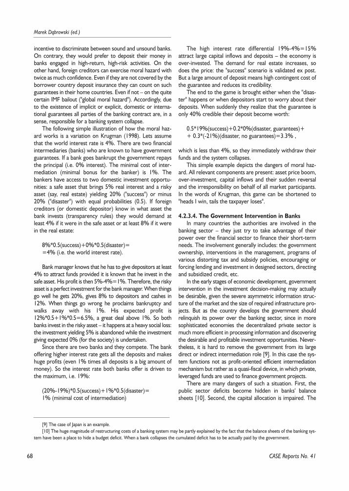
68
Marek D¹browski (ed.)
incentive to discriminate between sound and unsound banks.On contrary, they would prefer to deposit their money inbanks engaged in high-return, high-risk activities. On theother hand, foreign creditors can exercise moral hazard withtwice as much confidence. Even if they are not covered by theborrower country deposit insurance they can count on suchguarantees in their home countries. Even if not – on the quitecertain IMF bailout ("global moral hazard"). Accordingly, dueto the existence of implicit or explicit, domestic or interna-tional guarantees all parties of the banking contract are, in asense, responsible for a banking system collapse.
The following simple illustration of how the moral haz-ard works is a variation on Krugman (1998). Lets assumethat the world interest rate is 4%. There are two financialintermediaries (banks) who are known to have governmentguarantees. If a bank goes bankrupt the government repaysthe principal (i.e. 0% interest). The minimal cost of inter-mediation (minimal bonus for the banker) is 1%. Thebankers have access to two domestic investment opportu-nities: a safe asset that brings 5% real interest and a riskyasset (say, real estate) yielding 20% ("success") or minus20% ("disaster") with equal probabilities (0.5). If foreigncreditors (or domestic depositor) know in what asset thebank invests (transparency rules) they would demand atleast 4% if it were in the safe asset or at least 8% if it werein the real estate:
8%*0.5(success)+0%*0.5(disaster)==4% (i.e. the world interest rate).
Bank manager knows that he has to give depositors at least4% to attract funds provided it is known that he invest in thesafe asset. His profit is then 5%-4%=1%. Therefore, the riskyasset is a perfect investment for the bank manager. When thingsgo well he gets 20%, gives 8% to depositors and cashes in12%. When things go wrong he proclaims bankruptcy andwalks away with his 1%. His expected profit is12%*0.5+1%*0.5=6.5%, a great deal above 1%. So bothbanks invest in the risky asset – it happens at a heavy social loss:the investment yielding 5% is abandoned while the investmentgiving expected 0% (for the society) is undertaken.
Since there are two banks and they compete. The bankoffering higher interest rate gets all the deposits and makeshuge profits (even 1% times all deposits is a big amount ofmoney). So the interest rate both banks offer is driven tothe maximum, i.e. 19%:
(20%-19%)*0.5(success)+1%*0.5(disaster)=1% (minimal cost of intermediation)
The high interest rate differential 19%-4%=15%attract large capital inflows and deposits – the economy isover-invested. The demand for real estate increases, sodoes the price: the "success" scenario is validated ex post.But a large amount of deposit means high contingent cost ofthe guarantee and reduces its credibility.
The end to the game is brought either when the "disas-ter" happens or when depositors start to worry about theirdeposits. When suddenly they realize that the guarantee isonly 40% credible their deposit become worth:
0.5*19%(success)+0.2*0%(disaster, guarantees)++ 0.3*(-21%)(disaster, no guarantees)=3.3% ,
which is less than 4%, so they immediately withdraw theirfunds and the system collapses.
This simple example depicts the dangers of moral haz-ard. All relevant components are present: asset price boom,over-investment, capital inflows and their sudden reversaland the irresponsibility on behalf of all market participants.In the words of Krugman, this game can be shortened to"heads I win, tails the taxpayer loses".
4.2.3.4. The Government Intervention in BanksIn many countries the authorities are involved in the
banking sector – they just try to take advantage of theirpower over the financial sector to finance their short-termneeds. The involvement generally includes: the governmentownership, interventions in the management, programs ofvarious distorting tax and subsidy policies, encouraging orforcing lending and investment in designed sectors, directingand subsidized credit, etc.
In the early stages of economic development, governmentintervention in the investment decision-making may actuallybe desirable, given the severe asymmetric information struc-ture of the market and the size of required infrastructure pro-jects. But as the country develops the government shouldrelinquish its power over the banking sector, since in moresophisticated economies the decentralized private sector ismuch more efficient in processing information and discoveringthe desirable and profitable investment opportunities. Never-theless, it is hard to remove the government from its largedirect or indirect intermediation role [9]. In this case the sys-tem functions not as profit-oriented efficient intermediationmechanism but rather as a quasi-fiscal device, in which private,leveraged funds are used to finance government projects.
There are many dangers of such a situation. First, thepublic sector deficits become hidden in banks' balancesheets [10]. Second, the capital allocation is impaired. The
CASE Reports No. 41
[9] The case of Japan is an example.[10] The huge magnitude of restructuring costs of a banking system may be partly explained by the fact that the balance sheets of the banking sys-
tem have been a place to hide a budget deficit. When a bank collapses the cumulated deficit has to be actually paid by the government.
69
Currency Crises in Emerging Markets – Selected Comparative ...
private entrepreneurs' access to bank funding becomes lim-ited (higher interest rates). The government involvementdiscourages the development of market based credit riskanalysis, appropriate screening and monitoring culture, andweakens a financial discipline and the quality of law enforce-ment in general. For example, a government supportextended to an insolvent bank is a precedent on whichexpectations of future bailouts are built. Bank managersmight act as having an implicit government guarantee withall the consequences. The government also often encour-ages banks to borrow abroad in foreign currency (by whichthey assume an exchange rate risk) because it eases thepressure on official foreign reserves and postpones the needof policy adjustment. Also it is to the authorities' advantage(although not to the banking system's advantage) not toencourage the transparency and prudent disclosure prac-tices – the less the public knows about the distortionarygovernment involvement, the more funds it is willing to pro-vide for the system. In the same manner, supervisors areoften discouraged by the government from intervening as itwould bring problems out and cause expenditure (to fix thesystem and recapitalize it). As a result, due to lack of trans-parency and improper supervision, it is difficult to assess thetrue condition of corporations and banks. Profits are over-stated while the scale of bad loans underestimated.
The government involvement significantly increases thevulnerability of the system, although the magnitude of thisvulnerability is not usually known until it is too late. In goodtimes, such a system can function without any obviousproblems: economic growth induce steady inflow of newdeposits but when the downturn comes the condition ofthe banking system deteriorates rapidly due to a rise in non-performing loans and a general deterioration of the assetquality.
4.2.3.5. Financial System and Financial LiberalizationFinancial system failures are often the effect of an
increased vulnerability that is connected to some regimechange, induced by a policy change or by external condi-tions. One type of such regime change is privatization butthe most important one is financial system liberalization andderegulation. This is usually associated with simultaneouscapital account liberalization.
In regime of financial repression, the authorities forcefinancial institutions to maintain low or even negative realinterest rate. There are limits on deposit and lending rates.It is impossible for the bank to charge large risk premia andthe opportunities for optimal but more risky investment areforegone. Constraints on the financial sector reduce (pri-vate) savings, distort investment and decrease the availabil-
ity of resources to finance capital accumulation and growth.On the other hand, well developed and liberal financial mar-kets help diversify risk (making high-risk and high-returninvestment attractive to investors), pool liquidity risk, prop-erly screen and monitor loan applications and bring aboutgeneral improvement of resources allocation. There isample evidence that financial development is positively cor-related with contemporaneous and future growth rates.
The bank life is actually very easy in the state of financialrepression. Because interest rates are artificially low thereare more possible borrowers than credit available – creditrationing takes place and banks comfortably cash in theirprofits. When the liberalization comes, the whole situationchanges. Bank management lacks experience necessary torun the business in the new environment. The nature of theregime change is the fact that it alters the incentives facingbanks and increases the risk of traditional behavior. First, byremoving interest limits and allowing new entrants, the lib-eralization drastically increases sector's competitiveness:traditional monopolistic profit disappears and banks have tostruggle for market share. Deregulation is often accompa-nied by a rapid growth of little regulated, aggressive non-bank financial institutions. Because they are allowed to con-duct activities, which banks are restrained from engaging in,they quickly outperform domestic banks both in attractingdeposits and lending expansion. As profit margins narrow,managers start to favor risky lending practices. Indeed,financial liberalization increases the risk-taking opportunitiessignificantly – not only there are new banking products andderivatives available but the system is open to yet unknownand unfamiliar types of opportunistic behavior facilitated bytemporary relaxed law enforcement.
The overall level of interest rates can become veryvolatile after liberalization (the removal of the interestrate ceilings) – often the rate remains high in the periodafter liberalization [11] and thus banks become more vul-nerable. As a result, they might prefer to borrow abroadand on-lend the hard currency to its customers (changingthe exchange rate risk into a credit risk, as it was men-tioned above). The problem is aggravated by a significantcapital inflow induced by the parallel process of capitalaccount liberalization. In the environment of capital abun-dance, inexperienced banks expand risky activitiesbeyond their ability to manage them properly. Both regu-lators and banks usually have limited knowledge concern-ing the complex instruments of the financial market whatcauses hardships with evaluation of the asset quality andposes a threat to balance sheets.
The popular term "sequential liberalization" is given as ananswer to the problem. In this view, the liberalization should
CASE Reports No. 41
[11] This was the case in some transition economies and also, for example, in Chile where real lending rates averaged 77% in the period1975–1982.
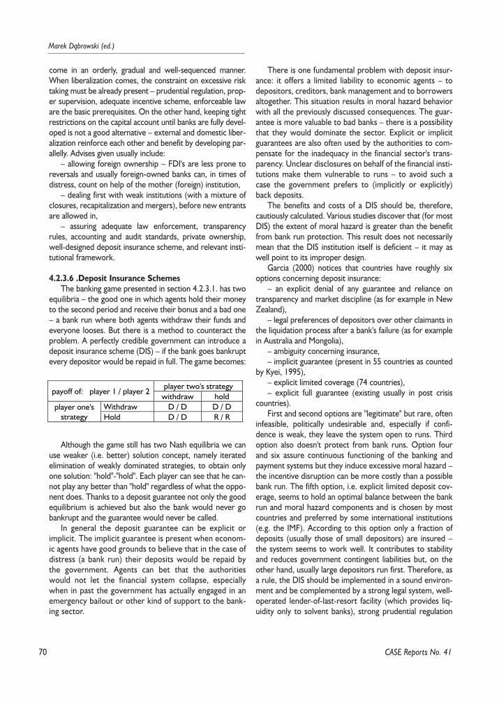
70
Marek D¹browski (ed.)
come in an orderly, gradual and well-sequenced manner.When liberalization comes, the constraint on excessive risktaking must be already present – prudential regulation, prop-er supervision, adequate incentive scheme, enforceable laware the basic prerequisites. On the other hand, keeping tightrestrictions on the capital account until banks are fully devel-oped is not a good alternative – external and domestic liber-alization reinforce each other and benefit by developing par-allelly. Advises given usually include:
– allowing foreign ownership – FDI's are less prone toreversals and usually foreign-owned banks can, in times ofdistress, count on help of the mother (foreign) institution,
– dealing first with weak institutions (with a mixture ofclosures, recapitalization and mergers), before new entrantsare allowed in,
– assuring adequate law enforcement, transparencyrules, accounting and audit standards, private ownership,well-designed deposit insurance scheme, and relevant insti-tutional framework.
4.2.3.6 .Deposit Insurance SchemesThe banking game presented in section 4.2.3.1. has two
equilibria – the good one in which agents hold their moneyto the second period and receive their bonus and a bad one– a bank run where both agents withdraw their funds andeveryone looses. But there is a method to counteract theproblem. A perfectly credible government can introduce adeposit insurance scheme (DIS) – if the bank goes bankruptevery depositor would be repaid in full. The game becomes:
Although the game still has two Nash equilibria we canuse weaker (i.e. better) solution concept, namely iteratedelimination of weakly dominated strategies, to obtain onlyone solution: "hold"-"hold". Each player can see that he can-not play any better than "hold" regardless of what the oppo-nent does. Thanks to a deposit guarantee not only the goodequilibrium is achieved but also the bank would never gobankrupt and the guarantee would never be called.
In general the deposit guarantee can be explicit orimplicit. The implicit guarantee is present when econom-ic agents have good grounds to believe that in the case ofdistress (a bank run) their deposits would be repaid bythe government. Agents can bet that the authoritieswould not let the financial system collapse, especiallywhen in past the government has actually engaged in anemergency bailout or other kind of support to the bank-ing sector.
There is one fundamental problem with deposit insur-ance: it offers a limited liability to economic agents – todepositors, creditors, bank management and to borrowersaltogether. This situation results in moral hazard behaviorwith all the previously discussed consequences. The guar-antee is more valuable to bad banks – there is a possibilitythat they would dominate the sector. Explicit or implicitguarantees are also often used by the authorities to com-pensate for the inadequacy in the financial sector's trans-parency. Unclear disclosures on behalf of the financial insti-tutions make them vulnerable to runs – to avoid such acase the government prefers to (implicitly or explicitly)back deposits.
The benefits and costs of a DIS should be, therefore,cautiously calculated. Various studies discover that (for mostDIS) the extent of moral hazard is greater than the benefitfrom bank run protection. This result does not necessarilymean that the DIS institution itself is deficient – it may aswell point to its improper design.
Garcia (2000) notices that countries have roughly sixoptions concerning deposit insurance:
– an explicit denial of any guarantee and reliance ontransparency and market discipline (as for example in NewZealand),
– legal preferences of depositors over other claimants inthe liquidation process after a bank's failure (as for examplein Australia and Mongolia),
– ambiguity concerning insurance,– implicit guarantee (present in 55 countries as counted
by Kyei, 1995),– explicit limited coverage (74 countries),– explicit full guarantee (existing usually in post crisis
countries).First and second options are "legitimate" but rare, often
infeasible, politically undesirable and, especially if confi-dence is weak, they leave the system open to runs. Thirdoption also doesn't protect from bank runs. Option fourand six assure continuous functioning of the banking andpayment systems but they induce excessive moral hazard –the incentive disruption can be more costly than a possiblebank run. The fifth option, i.e. explicit limited deposit cov-erage, seems to hold an optimal balance between the bankrun and moral hazard components and is chosen by mostcountries and preferred by some international institutions(e.g. the IMF). According to this option only a fraction ofdeposits (usually those of small depositors) are insured –the system seems to work well. It contributes to stabilityand reduces government contingent liabilities but, on theother hand, usually large depositors run first. Therefore, asa rule, the DIS should be implemented in a sound environ-ment and be complemented by a strong legal system, well-operated lender-of-last-resort facility (which provides liq-uidity only to solvent banks), strong prudential regulation
CASE Reports No. 41
player two's strategypayoff of: player 1 / player 2
withdraw holdWithdraw D / D D / Dplayer one's
strategy Hold D / D R / R
71
Currency Crises in Emerging Markets – Selected Comparative ...
and supervision [12]. Most importantly the DIS has to havepublic confidence.
The situation changes somehow during crises. Limitedcoverage cannot be expected to support the stability of thesystem in the presence of a large shock. In this case author-ities should offer a full but explicitly temporary guaranteesto assure the continued functioning of the financial system.
4.2.3.7. The Basle Capital AccordThe so-called Basle Capital Accord was initiated in 1988.
Originally regarding the G10 countries' banks (only thoseoperating internationally) has since became a widely accept-ed standard for the evaluation of banks' financial soundnessand is applied to all banks. Accord has been designed tocounteract the decline of banks' capital observed for muchof the 20th century. It is based on the risk-weighted assets.The simple risk measurement includes four risk-categorieswith assigned weights ranging from 0 to 100%, dependingon the credit risk of the borrower. For example, loans tocommercial companies are weighted 100%, interbank lend-ing 20% while loans to central government in local curren-cy (virtually riskless) – 0%. The Accord requires banks tomaintain its capital equivalent to at least 8% of such risk-weighted assets. This framework has the advantage of beinga simple and comparable measure of bank soundness but,on the other hand, it neither makes any adjustment for riskdiversification, nor is sophisticated enough to adequatelyprice the new complex banking instruments. Since theAccord was designed for stable industrialized countries withdeveloped and well-established financial systems, countrieswith volatile and risky macroeconomic environment shouldaccordingly implement higher capital adequacy ratios –indeed, most of them do.
The Accord has been, in general, successful in reversingthe trend of banks' decapitalization in most of G10 countriesand assuring the (relative) bank soundness elsewhere.
4.3. Assessing the Condition of a BankingSystem
The theory offers guidance as what are the determi-nants of banking crisis and allows building the framework toassess the quality of a banking sector and its vulnerability toa crisis.
The "bottom-up" approach analyzes each individual bankand then sum up the scores to obtain the result for the
whole banking system while the "aggregate" approach mea-sures the probability of systemic insolvency using the aggre-gate banking sector data with similar methodology as in thecase of individual bank. As a complementary method, the"macroeconomic" approach can be applied – it relies on thefact that bank's solvency depends on the state of their cus-tomers what in turn depends on the condition of the econ-omy – it therefore tries to establish links between macro-economic indicators and bank soundness.
Typically the bank's condition would be assessed byidentifying the relevant indicators that are correlated withvariables responsible for bank's solvency. These indicators,generally, fall into five categories:
The first is exposure to risk – among this group a usefulindicators include:
– Loan to deposit ratio, as a measure of bank's leverageand the extent to which bank relies on other, nontradition-al sources of funding. When times are good banks wouldseek to increase its leverage to maximize profits, but areversal of economic trend is much more dangerous forhighly leveraged companies.
– The ratio of non-performing loans is a (somehow ex-post) measure of en exposure to credit risk – increase inNPL means that a bank would have to provision for expect-ed losses – its capital base erodes. High ratios points toinadequate lending practices and bad risk pricing – Sheng(1996) notices that a collapse is rather inevitable when thisratio exceeds (provisioning by) 15%.
– Exposure to real estate and equity market measuresthe extent of market risk a bank is taking. In the event of asharp decline in asset prices the bank can easily go insolvent.The difference between current and trend values of assetprices multiplied by the exposure provides a good measure.High ratios also indicate that the bank's core business is lessprofitable.
– Net open foreign exchange position measures theexposure to exchange rate risk. In an event of unexpecteddevaluation the bank is going to incur heavy losses.
The second includes solvency conditions – they explicit-ly take into account the adequacy of banks capital – the (riskweighted) capital adequacy ratio (actual and projected)should be sufficient (minimum 8% according to the BasleCommittee) to assure that the bank has enough capacity toabsorb possible losses [13].
The third consist of liquidity criteria:– Lender of last resort indicator – the more often a bank
has to resort to the central bank's credit the more probableis its insolvency. Sound banks shouldn't have systemic prob-
CASE Reports No. 41
[12] Another question is whether the DIS should be public or private. The United Kingdom has a private system while the US has government-run system which is privately funded but has explicit government support. Other countries have mostly public guarantees.
[13] Interestingly enough, the run-up to the Mexican financial crisis was accompanied by the almost perfect capital adequacy in the banking system.
72
Marek D¹browski (ed.)
lems with liquidity and should be able to fund themselves onthe interbank market. If the bank is cut from the interbankfunding or faces above average interest rates it is a clear signthat something is wrong with the bank (the manager, forexample, may be known to the market to be an excessiverisk taker). Also compliance to statutory reserve require-ments or liquid asset requirements is a good indicator of thesame kind.
The fourth is profitability – usually measured by returnon assets. The likelihood of remaining solvent depends, ofcourse, on bank's profitability. A decline in that indicatorshould be an important warning signal. Low interest marginsalso indicate problems. Similarly a significant share of non-interest income in total income may point to the weaknessin the core banking business. The performance of bank'sshares can reveal much about the future prospects of thebank as well.
Finally, there is a "supervisory assessment" criterion – theofficial assessment of banks' condition should be taken intoaccount. The evaluation can be in a form of a standardCAMEL rating (based on Capital adequacy, Asset quality,adequacy of Management, Earnings, Liquidity); alternatively,some supervisory bodies construct a so-called watch listincorporating banks that should take corrective measure toimprove their standing.
Judging from the macroeconomic and aggregateapproach, a rapid growth of aggregate bank lending to realestate and equity sectors is a classic leading indicator of acrisis. Similarly, the aggregate inflow of portfolio capitalexceeding, say, 10% of GDP over a couple of years alsoindicates increased vulnerability. The dim prospects forthe economy and the expected growth slowdown con-tribute to the worsening of the banking system through itsimpact on banks' clients. The microeconomic structureshould also be taken into account: the design of the DIS,the quality of supervision, and the degree of ownershipconcentration are relevant variables. The involvement ofthe government in the banking system, political and con-nected lending, management's reckless or fraudulentbehavior are almost always accompanied by market gos-sips and rumors and through this can be incorporated intothe analysis.
High liquidity can offset financial system problems – aslong as there is a capital to intermediate the system can func-tion. The possible monetary tightening in major developedcountries should be a particularly important indicator [14].
The above-sketched framework is frequently used toconstruct the so-called early warning systems [15].
4.4. Empirical Evidence and the Determi-nants of Banking and Currency Crises
4.4.1. Banking Crises in the Real World
The endogenous boom-bust cycle banking sector crisistheory is consistent with the experiences of Argentina,Chile, Uruguay 1979–1983, Japan in the 1990s, Nordiccountries 1987–94, Mexico 1994 and Asia 1997–1998. Inevery country there was a significant economic boomaccompanied with rapid increase in credit.
The so-called "debt crisis" in early 1980s was precededby a surge in international lending to emerging markets at avery low interest rate. The heavy lending caused consump-tion boom (financed by expansion of bank credit), an assetprice bubble, a real appreciation, a current account deficits,etc. When industrial countries engaged in tight anti-infla-tionary policies the debtors could no longer respect theirobligations, defaulted and went into a crisis.
The Asian crisis included similar dynamics, but ratherinstead of the consumption boom there was an excessiveinvestment. Over-lending, over-investment and moral haz-ard were engraved by the initial success of this policy –widely shared optimism about future growth based on along tradition without a single year of negative growth. Lastyear with growth rate of significantly lower than 5% was inIndonesia in 1985, in Malaysia in 1986, in Korea in 1980 andin Thailand in 1972. The crisis was, again, triggered by a sud-den outflow of foreign capital. However, the collapse of thefinancial system was far more damaging in Asian economiesdue to a deeper financial markets, higher debt-equity andcredit-GDP ratios. Similarly, the degree of overvaluation inAsia was smaller, but due to relative openness of theseeconomies the results of the overvaluation were moresevere.
On the other hand, the 1999 Brazilian crisis was not afinancial crisis but rather a classic balance of payment crisiswith unsustainable fiscal policy. The banking system wassound, adequately hedged and capitalized. The relationshipbetween the soundness of the banking sector and the sever-ity of crises is, therefore, evident.
As we mentioned before, the soundness of the financialsystem depends on the quality of the supervision and theenforcement of prudential rules – especially in the period offinancial liberalization.
In Korea the liberalization started in 1991, in 1993 short-term interest rates and in 1994 lending rates were deregu-
CASE Reports No. 41
[14] Although the 1997–98 Asian crisis (as opposite to the 1994–95 Mexican crisis of 1994–95) erupted when the international liquidity was high.[15] It should be said that not only the state of the banking sector but also the condition of the corporate sector (analogously: the moral hazard,
increased leverage, unhedged borrowing, overinvestment, political connections) should be taken into account in estimating the probability of a cur-rency or a full-fledged financial crisis in a given country.

73
Currency Crises in Emerging Markets – Selected Comparative ...
lated. Rapid growth of non-bank financial intermediaries –investment and finance companies, mutual savings and mer-chant banking corporations – followed. They enjoyed agreater autonomy and were able to offer higher interestrates on deposits. Non-commercial bank share in "deposits"rose from 37% at end-1980 to 68% by June 1995. Theyquickly developed serious maturity and currency mismatch-es; for example, by 1997 over 70% of their funding wereshort-term while 90% of loans were long-term. Despitethis fact, the supervision was weak and fragmented (Bank ofKorea supervised commercial banks while the Ministry ofFinance supervised merchant banks); provisioning was evenrelaxed in 1995–95 (from 100 to 75% for doubtful loans).Korean Deposit Insurance Corporation only was estab-lished in 1996.
In Indonesia, between 1978 and 1995, the number ofbanks doubled. Regulatory and legal structure was simplyunable to manage banking business in much more compli-cated environment.
In Thailand, the number of non-bank financial interme-diaries exploded as well – they conducted activities, whichbanks were restrained from engaging in. Supervision wasagain fragmented between the Bank of Thailand and theMinistry of Finance. Rules for loan classification were oftenignored, large portfolios of questionable loans were simplyrolled-over rather than classified as non-performing. Therewere no limits of large exposures to corporate groups.
Deregulation was accompanied by the rapid growth oflittle regulated non-bank financial institutions in other coun-tries as well – in Chile from 1974, Argentina since 1978,Venezuela before 1989 – to name a few. For example, inChile in early 1970s, following privatization, new "groupos"i.e. large conglomerates emerged. They were aggressive,highly leveraged and centered around few banks; by 1979they controlled more than 80% of all private banks andalmost 70% of the equity of firms listed in the stockexchange. Banks acted as agents for these groups andengaged in risky, connected lending, despite their weak cap-ital position.
The above-described syndrome is not unique to emerg-ing markets only. For example, in Sweden, since the end ofthe WWII the banking system was a very regulated.Between 1945 and 1983 there were no new privateentrants. The objective was to avoid banking system fail-ures. In 1986 one prominent Swedish economist said thatthe idea of a bank run or collapse was out of the question.There has also been a long-tradition of close relationshipbetween industry and banking sector. Swedish banks as wellas regulatory bodies were not prepared for liberalization.Tranquil and profitable existence in the environment ofcredit rationing and monopolistic profit turned into a hardlife of increased competition and rising complexity of finan-cial instruments. The new "direct finance" sector emerged.Banks, as previously, had to maintain high capital adequacy
ratios while new non-bank entrants not. These lightly regu-lated institutions engaged in leveraged real estate lending.The asset bubble finally burst and between 1988 and 1990half of finance companies went bankrupt. The impairmentof the Swedish banking system prolonged several years. Toa large extent, the crisis was a result of inadequate supervi-sion and prudential regulations.
According go the World Bank (1993), inadequate pru-dential regulations also played a major role in crises inHong-Kong, 1982–1983, Japan, 1991, Chile, 1981–1993,the Philippines, 1981–1987, Turkey, 1982–1985, the US1979–1989 and many more.
In the same spirit, after the Asian crisis, Bank of Koreaadmitted that moral hazard (caused by government guaran-tees) had been present in the case of all major players onthe financial markets: borrowers, financial institutions, theircreditors and depositors. For example, the President oncesaid that Korean financial institutions were immune to fail-ure because government implicitly guaranteed their solven-cy and liquidity. And, indeed, the general opinion was thatthe government would not allow commercial and merchantbanks go bankrupt.
By arranging a bailout the government proved that eco-nomic agents were right in their expectations (implicit guar-antee). This only reinforced these expectations and wors-ened the moral hazard problem. For example, the Chilean"groupos" started to experience difficulties in early-1980s.Nevertheless, there were expectation of governmentbailout, and indeed, in 1983, after two largest groupos wentbankrupt the government took over five banks, amongthem the two largest – owned by the conglomerates.Implicit guarantees in the banking system were evidentbefore the Asian crisis – although only Korea and Thailandhad explicit deposit insurance schemes, up to 1993 onlyHong Kong and Thailand closed any insolvent intermedi-aries. Major government support has been extended to thefailed banking institutions in Malaysia 1985–1988, Thailand1983–1987, Philippines 1981–1987 and others – theinvestors and depositors had good grounds to believe that itwould happen again in the future, if necessary.
Investors took a specific lesson of global moral hazard inearly 1995. Holders of dollar denominated Mexican bondswere bailed-out by the IMF and other financial institutionswhile holders of other forms of Mexican papers, equity andmost peso denominated papers in particular, did suffer heavylosses. This event most probably distorted the patterns ofinternational capital flows – there was a change from equityto debt and from domestic to hard currency. Interbank lend-ing grew in importance, in the expense of equity. This meansthat debt became very short-term and denominated in for-eign currency. Interbank lending to five most crisis-affectedcountries in Asia ran at around 43$bln a year. Before the1997–1998 crisis, about 40% were denominated in yen, therest in USD; 2/3 had maturity less than a year.
CASE Reports No. 41
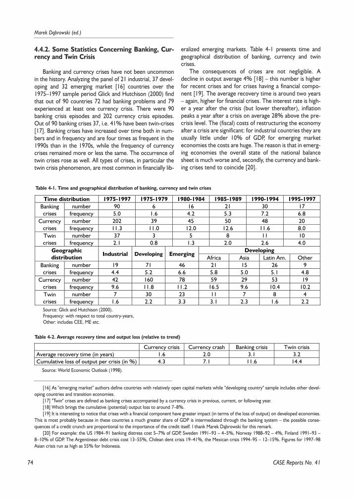
74
Marek D¹browski (ed.)
4.4.2. Some Statistics Concerning Banking, Cur-rency and Twin Crisis
Banking and currency crises have not been uncommonin the history. Analyzing the panel of 21 industrial, 37 devel-oping and 32 emerging market [16] countries over the1975–1997 sample period Glick and Hutchison (2000) findthat out of 90 countries 72 had banking problems and 79experienced at least one currency crisis. There were 90banking crisis episodes and 202 currency crisis episodes.Out of 90 banking crises 37, i.e. 41% have been twin-crises[17]. Banking crises have increased over time both in num-bers and in frequency and are four times as frequent in the1990s than in the 1970s, while the frequency of currencycrises remained more or less the same. The occurrence oftwin crises rose as well. All types of crises, in particular thetwin crisis phenomenon, are most common in financially lib-
eralized emerging markets. Table 4-1 presents time andgeographical distribution of banking, currency and twincrises.
The consequences of crises are not negligible. Adecline in output average 4% [18] – this number is higherfor recent crises and for crises having a financial compo-nent [19]. The average recovery time is around two years– again, higher for financial crises. The interest rate is high-er a year after the crisis (but lower thereafter), inflationpeaks a year after a crisis on average 28% above the pre-crisis level. The (fiscal) costs of restructuring the economyafter a crisis are significant: for industrial countries they areusually little under 10% of GDP, for emerging marketeconomies the costs are huge. The reason is that in emerg-ing economies the overall state of the national balancesheet is much worse and, secondly, the currency and bank-ing crises tend to coincide [20].
CASE Reports No. 41
[16] As "emerging market" authors define countries with relatively open capital markets while "developing country" sample includes other devel-oping countries and transition economies.
[17] "Twin" crises are defined as banking crises accompanied by a currency crisis in previous, current, or following year.[18] Which brings the cumulative (potential) output loss to around 7–8%.[19] It is interesting to notice that crises with a financial component have greater impact (in terms of the loss of output) on developed economies.
This is most probably because in these countries a much greater share of GDP is intermediated through the banking system – the possible conse-quences of a credit crunch are proportional to the importance of the credit itself. I thank Marek D¹browski for this remark.
[20] For example: the US 1984–91 banking distress cost 5–7% of GDP, Sweden 1991–93 – 4–5%, Norway 1988–92 – 4%, Finland 1991–93 –8–10% of GDP. The Argentinean debt crisis cost 13–55%, Chilean dent crisis 19–41%, the Mexican crisis 1994–95 – 12–15%. Figures for 1997–98Asian crisis run as high as 55% for Indonesia.
Table 4-1. Time and geographical distribution of banking, currency and twin crises
Time distribution 1975-1997 1975-1979 1980-1984 1985-1989 1990-1994 1995-1997number 90 6 16 21 30 17Banking
crises frequency 5.0 1.6 4.2 5.3 7.2 6.8number 202 39 45 50 48 20Currency
crises frequency 11.3 11.0 12.0 12.6 11.6 8.0number 37 3 5 8 11 10Twin
crises frequency 2.1 0.8 1.3 2.0 2.6 4.0DevelopingGeographic
distributionIndustrial Developing Emerging
Africa Asia Latin Am. Othernumber 19 71 46 21 15 26 9Banking
crises frequency 4.4 5.2 6.6 5.8 5.0 5.1 4.8number 42 160 78 59 29 53 19Currency
crises frequency 9.6 11.8 11.2 16.5 9.6 10.4 10.2number 7 30 23 11 7 8 4Twin
crises frequency 1.6 2.2 3.3 3.1 2.3 1.6 2.2Source: Glick and Hutchison (2000).Frequency: with respect to total country-years,Other: includes CEE, ME etc.
Table 4-2. Average recovery time and output loss (relative to trend)
Currency crisis Currency crash Banking crisis Twin crisisAverage recovery time (in years) 1.6 2.0 3.1 3.2Cumulative loss of output per crisis (in %) 4.3 7.1 11.6 14.4
Source: World Economic Outlook (1998).
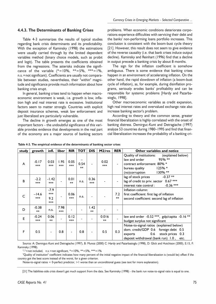
75
Currency Crises in Emerging Markets – Selected Comparative ...
4.4.3. The Determinants of Banking Crises
Table 4-3 summarizes the results of typical studiesregarding bank crisis determinants and its predictability.With the exception of Kaminsky (1998) the estimationswere usually carried through by the limited dependentvariables method (binary choice models, such as probitand logit). The table presents the coefficients obtainedfrom the regressions. The asterisks indicate the signifi-cance of the variable (*=10%, **=5%, ***=1%,n.s.=not significant). Coefficients are usually not compara-ble between studies, nevertheless, their "within" magni-tude and significance provide much information about howbanking crisis erupt.
In general, banking crises tend to happen when macro-economic environment is weak, i.e. growth is low, infla-tion high and real interest rate is excessive. Institutionalfactors seem to matter strongly. Countries with explicitdeposit insurance schemes, weak law enforcement andjust liberalized are particularly vulnerable.
The decline in growth emerges as one of the mostimportant factors – the undoubtful significance of this vari-able provides evidence that developments in the real partof the economy are a major source of banking sectors
problems. When economic conditions deteriorate corpo-rations experience difficulties with servicing their debt andthe banks' non-performing loans portfolio increases. Thisconclusion is consistent with the boom-bust cycle theory[21]. However, this result does not seem to give evidenceof the reverse causality (i.e. that bank crises induce outputdecline). Kaminsky and Reinhart (1996) find that a declinein output precede a banking crisis by about 8 months.
The sign for the inflation coefficient is somehowambiguous. There is some evidence that banking criseshappen in an environment of accelerating inflation. On theother hand, the rapid slowdown of inflation (a boom-bustcycle of inflation), as, for example, during disinflation pro-grams, seriously erodes banks' profitability and can beresponsible for systemic problems [Hardy and Pazarba-sioglu, 1998].
Other macroeconomic variables as credit expansion,high real interest rates and overvalued exchange rate alsoincrease banking sector's problem.
According to theory and the common sense, greaterfinancial liberalization is highly correlated with the onset ofbanking distress. Demirguc-Kunt and Detragiache (1997)analyze 53 countries during 1980–1995 and find that finan-cial liberalization increases the probability of a banking cri-
CASE Reports No. 41
[21] The liabilities-side crisis doesn't get much support from the data. See Kaminsky (1998) - the bank run noise-to-signal ratio is equal to one.
Table 4-3. The empirical evidence of the determinants of banking sector crises
study growth infl. liber RIR TOT DIS M2/res RER Other variables and notice
A-0.17***
0.03***
1.95***
0.05***
–0.54**
-0.02***
-
Quality of institutions: (explained below)law and order 95% **contract enforcement 80% *bureau quality 125% *(no)corruption 130% **
B-2.2***
-1.42***
-0.01**
n.s.0.36***
- -lag of stock prices -0.37 **lag of credit to priv. sector 0.67 ***interest rate control : -0.36 ***
C–14.6***
-7.9***9.2***
-0.06***
n.s. - -7.2**
Inflation column:first coefficient: first lag of inflationsecond coefficient: second lag of inflation
D-0.38
**n.s.
7.98***
- -1.42**
- -
E-0.24***
0.06**
-0.12***
- -0.016
**-
law and order -0.52 ***, gdp/capita -0.16 **budget surplus not significant
F 0.5 - 0.8 - 0.8 - 0.5 0.3
Noise-to-signal ratios (explained below)dom. credit/GDP 0.6 foreign debt 0.5exports 0.6 stock prices 0.3deposit withdrawal (bank run) 1.0 , etc.
Source: A: Demirguc-Kunt and Detragiache (1997), B: Munoz (2000) C: Hardy and Pazarbasioglu (1998), D: Glick and Hutchison (2000), E:15, F:Kaminsky (1998).
"-"=not included, n.s.=not significant, *=10%, **=5%, ***=1%"Quality of institution" coefficient indicates how many percent of the initial negative impact of the financial liberalization is (would be) offset if the
country got the best score instead of the worst, for a given criterion.Noise-to-signal ratios = 0-perfect predictor, >1 worse than an unconditional guess (see text for more explanation).
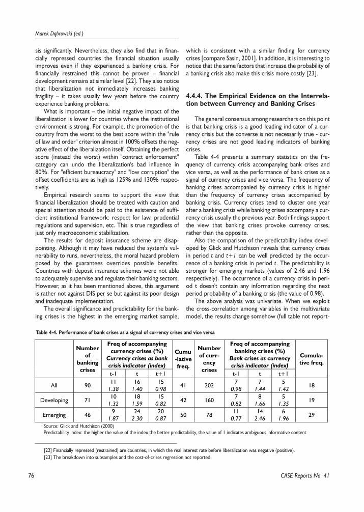
76
Marek D¹browski (ed.)
sis significantly. Nevertheless, they also find that in finan-cially repressed countries the financial situation usuallyimproves even if they experienced a banking crisis. Forfinancially restrained this cannot be proven – financialdevelopment remains at similar level [22]. They also noticethat liberalization not immediately increases bankingfragility – it takes usually few years before the countryexperience banking problems.
What is important – the initial negative impact of theliberalization is lower for countries where the institutionalenvironment is strong. For example, the promotion of thecountry from the worst to the best score within the "ruleof law and order" criterion almost in 100% offsets the neg-ative effect of the liberalization itself. Obtaining the perfectscore (instead the worst) within "contract enforcement"category can undo the liberalization's bad influence in80%. For "efficient bureaucracy" and "low corruption" theoffset coefficients are as high as 125% and 130% respec-tively.
Empirical research seems to support the view thatfinancial liberalization should be treated with caution andspecial attention should be paid to the existence of suffi-cient institutional framework: respect for law, prudentialregulations and supervision, etc. This is true regardless ofjust only macroeconomic stabilization.
The results for deposit insurance scheme are disap-pointing. Although it may have reduced the system's vul-nerability to runs, nevertheless, the moral hazard problemposed by the guarantees overrides possible benefits.Countries with deposit insurance schemes were not ableto adequately supervise and regulate their banking sectors.However, as it has been mentioned above, this argumentis rather not against DIS per se but against its poor designand inadequate implementation.
The overall significance and predictability for the bank-ing crises is the highest in the emerging market sample,
which is consistent with a similar finding for currencycrises [compare Sasin, 2001]. In addition, it is interesting tonotice that the same factors that increase the probability ofa banking crisis also make this crisis more costly [23].
4.4.4. The Empirical Evidence on the Interrela-tion between Currency and Banking Crises
The general consensus among researchers on this pointis that banking crisis is a good leading indicator of a cur-rency crisis but the converse is not necessarily true - cur-rency crises are not good leading indicators of bankingcrises.
Table 4-4 presents a summary statistics on the fre-quency of currency crisis accompanying bank crises andvice versa, as well as the performance of bank crises as asignal of currency crises and vice versa. The frequency ofbanking crises accompanied by currency crisis is higherthan the frequency of currency crises accompanied bybanking crisis. Currency crises tend to cluster one yearafter a banking crisis while banking crises accompany a cur-rency crisis usually the previous year. Both findings supportthe view that banking crises provoke currency crises,rather than the opposite.
Also the comparison of the predictability index devel-oped by Glick and Hutchison reveals that currency crisesin period t and t+1 can be well predicted by the occur-rence of a banking crisis in period t. The predictability isstronger for emerging markets (values of 2.46 and 1.96respectively). The occurrence of a currency crisis in peri-od t doesn't contain any information regarding the nextperiod probability of a banking crisis (the value of 0.98).
The above analysis was univariate. When we exploitthe cross-correlation among variables in the multivariatemodel, the results change somehow (full table not report-
CASE Reports No. 41
[22] Financially repressed (restrained) are countries, in which the real interest rate before liberalization was negative (positive). [23] The breakdown into subsamples and the cost-of-crises regression not reported.
Table 4-4. Performance of bank crises as a signal of currency crises and vice versa
Freq of accompanyingcurrency crises (%)
Currency crises as bankcrisis indicator (index)
Freq of accompanyingbanking crises (%)
Bank crises as currencycrisis indicator (index)
Numberof
bankingcrises
t-1 t t+1
Cumu-lativefreq.
Numberof curr-
encycrises
t-1 t t+1
Cumula-tive freq.
All 9011
1.3816
1.4015
0.9841 202
70.98
71.44
51.42
18
Developing 7110
1.3218
1.5915
0.8242 160
70.82
81.66
51.35
19
Emerging 469
1.8724
2.3020
0.8750 78
110.77
142.46
61.96
29
Source: Glick and Hutchison (2000)Predictability index: the higher the value of the index the better predictability, the value of 1 indicates ambiguous informative content
77
Currency Crises in Emerging Markets – Selected Comparative ...
CASE Reports No. 41
ed). Currency crises as predictors of banking crisis remaininsignificant (except for contemporaneous events). Theusefulness of banking crises as predictors of currencycrises decreases substantially – they only issue a proper(and very strong) signal of an approaching currency crisis inthe case of emerging markets. The contemporaneous cor-relation is significant for both developing and emergingmarkets.
Kaminsky (1998) develops a so-called "signal approach"to assess what are the determinants of both currency andbanking crises. The estimated coefficient are actuallynoise-to-signal ratios (ntsr): the coefficient equal to zeroindicates perfect predictability power of the variable, thecoefficient one indicate the power of a simple uncondi-tional guess (i.e. the variable in question is neutral) whilevalues greater than one disqualify the variable. She noticesthat it is a little harder to predict banking crises (com-pounded ntsr=0.8) than currency crises (ntsr=0.7). Thebest variable to predict both crises is the real exchangerate overvaluation (ntsr=0.2 for currency crises and 0.3for banking crises). Consistently with other studies shefinds that a banking crisis is a very good indicator of a cur-rency crisis (ntsr=0.3) while the opposite is not true(ntsr=1.2).
4.5. Conclusions
It has been shown that banking crises and currencycrises are interrelated and that banking crises are goodleading indicators of currency crises, so there is a point inassessing the condition of the financial system and theprobability of a banking crisis. The recent crises are shownto follow the pattern of a boom-bust over-lending – over-investment cycle. Banking crises emerge when macroeco-nomic situation deteriorates, i.e. growth slows down, infla-tion and the real interest rates are high, etc.
Institutional factors matter: countries with explicitdeposit insurance scheme or with inadequate contractenforcement are more vulnerable. The financial liberaliza-tion increases the possibility of a crisis in improperly regu-lated banking sector. The problem of moral hazard chieflycontributes to the emergence of a crisis.
78
Marek D¹browski (ed.)
References
BIS 68th Annual Report, Basle.Berg A., C. Patillo (1999). "Are Currency Crises Pre-
dictable? A test, IMF/SP/46.Bisignano J. (1999). "Precarious Credit Equilibria:
Reflections on the Asian Financial Crisis, BIS/WP/64.Burnside C., M. Eichenbaum, S. Rebelo, "Prospective
Deficits and the Asian Currency Crisis, NBER.Calvo G., E. Mendoza (1996). "Mexico's Balance of Pay-
ments Crises. A chronicle of a Death Foretold". Journal ofInternational Economics, 41, 235–264.
Caprio G., D. Klingebiel (1996). "Bank Insolvencies:Cross-Country Experiences. WB/PRP/1620.
Chang R., A. Velasco (1999). "Liquidity Crises inEmerging Markets: Theory and Policy, NBER 7272.
Demirguc-Kunt A., E. Detragiache (1998). "The Deter-minants of Banking Crises: Evidence from Developing andDeveloped Countries". IMF/WP/97/106.
Demirguc-Kunt A., E. Detragiache (1998). "FinancialLiberalization and Financial Fragility". IMF/WP/98/93.
Demirguc-Kunt A., E. Detragiache, P. Gupta (2000)."Inside a Crisis: an Empirical Analysis of Banking System inDistress, IMF/WP/00/156.
Dekle R., K. Kletzer (2000). "Domestic Bank Regulationand Financial Crises: Theory and Empirical Evidence fromEast Asia". Mimeo., UCLA.
Diamond D., P. Dybvig (1983). "Bank Runs, DepositInsurance, and Liquidity". Journal of Political Economy, 91,401–19.
Diaz-Alejandro C. (1983). "Goodbye Financial Repres-sion, Hello Financial Crash". Journal of Development Eco-nomics, 19, pp. 1–24.
Dooley M. (1997). "A Model of Crises in EmergingMarkets". NBER/WP/6300.
Dornbusch R. (2001). "A Primer on Emerging MarketCrises". Mimeo., MIT.
Downes P., D. Marston, I. Otker (1999). "MappingFinancial Sector Vulnerability in a Non-crisis Country".IMF/PDP/99/4.
Edwards S., A. Cox-Edwards (1987). "Monetarism andLiberalization: the Chilean Experiment". Chicago.
Englund P. (1990). "Financial Deregulation in Sweden".European Economic Review.
Eichengreen B., A. Rose, Ch. Wyplosz (1995)."Exchange Market Mayhem. The Antecedents and After-math of Speculative Attacks". Economic Policy, 21, Octo-ber, 249–312.
Eichengreen B. (1999). "Toward a New InternationalFinancial Architecture: a Practical Post-Asia Agenda, IIE.
Frankel J., A. Rose (1996). "Currency Crashes inEmerging Markets. An Empirical Treatment". Journal ofInternational Economics, 41, November, 351–366.
Garcia G. (2000). "Deposit Insurance and Crisis Man-agement". IMF/WP/00/57.
Glick R., M. Hutchison (2000). "Banking and CurrencyCrises: how Common are the Twins?, Hong Kong Institutefor Monetary Research.
Hardy D., C. Pazarbasioglu (1998). "Leading Indicatorsof Banking Crises: Was Asia Different?" IMF/WP/98/91.
Honohan P. (1997). "Banking System Failures in Devel-oping and Transition Countries: Diagnosis and Prediction".BIS/WP/39.
Kaminsky G., C. Reinhart (1996). "The Twin Crises: theCauses of Banking and Balance of Payment Crises".FRB/IFDP/544.
Kaminsky G. (1998). "Currency and Banking Crises, theEarly Warning of Distress". FRB/IFDP/629.
McKinnon R., H. Pill (1999). "Was There a Boom inMoney and Credit Prior to East Asia's Recent CurrencyCrisis?. FRB of SF, Economic Review No. 1.
Kiyotaki N., J. Moore (1997). "Credit Cycles". Journalof Political Economy.
Krugman P. (1998). "What Happened to Asia?. Mimeo.,MIT.
Kyei A. (1995). "Deposit Protection Arrangements: aComparative Study". IMFWP/95/134.
Mishkin F. (2000). "Financial Policies and the Preventionof Financial Crises in Emerging Market Countries". NBER.
Munoz S. (2000). "The Breakdown of Credit Relationsunder Conditions of a Banking Crisis: a Switching RegimeApproach". IMF/WP/00/135.
Sachs J., A. Tornell, A. Velasco (1996). "Financial Crisesin Emerging Markets. The Lessons from 1995". BrookingsPapers on Economic Activity, No. 1, 147–215.
Sheng, A., ed. (1996). "Bank Restructuring". WB.Stiglitz J., A. Weiss (1981). "Credit Rationing in Markets
with Imperfect Information". The American EconomicReview.
Yieyati L. (1999). "Global Moral Hazard, CapitalAccount Liberalization and the "Overlending Syndrome".IMF/WP/99/100.
CASE Reports No. 41
79
Currency Crises in Emerging Markets – Selected Comparative ...
CASE Reports No. 41
5.I. Introduction
The recent wave of currency crises in the 1980s and1990s has led to a resumption of studies into this economicphenomenon. The series of crises started with the Mexicandebt crisis in 1982, followed by the European Monetary Sys-tem crisis of 1992–1993, the Mexico crisis of 1994, theAsian crisis of 1997, the Russian crisis of 1998 and theBrazilian crisis of 1999. The financial turmoil seen in thesecrises triggered a vast bulk of literature on various issuessurrounding the topic. Despite all the advancements in the-ory and empirical analyses there are still some unclearaspects. This ambiguity arises even with regard to the defi-nition of a crisis per se.
One strand of currency crisis theory deals with thecross-country propagation of crises – very often referred toas contagion. An investigation into the nature of this mecha-nism is of key importance for a proper understanding ofcrises. An understanding of contagion has very importantpolicy implications as it can help in the search for answers asto whether contagion can be stopped or avoided.
Despite the proliferation of literature on crisis propaga-tion in recent years there is no research consensus on issuessurrounding contagion. One of the reasons for this is theproblem of defining contagion in the first place. Notwith-standing intuitive comprehensions of the term contagion,numerous misconceptions arise. Since the inception of con-tagion theory, the term contagion has been used in a varietyof ways, covering both broad and narrow meanings. Thus,this paper starts with a survey of literature on contagion,focusing on definitional approaches. The focus is then shift-ed to the problem of identifying the various means by whichcrises propagation, followed by a look at measurementmethods.
Research to date has tended to take one of three routes:to investigate individual channel of contagion; to test empir-ically which channel is most important; to discover simplywhether there was any contagion at all. For instance, Mas-son (1998) and Masson (1999) explored a transmissionmechanism via multiple equilibria; Rijckeghem and Weder
(1999a) explored the common lender effect; Drazen (1999)explored political contagion; Glick and Rose (1999) lookedat trade channels, and Eichengreen et al. (1996) tested forcontagion and the importance of the trade channel. Forbesand Rigobon (1999b) have pointed out deficiencies ineconometric tests for contagion and proposed their owntest, which remains consistent with econometric theory.
The results of and conclusions drawn from the above-mentioned papers seem to depend to a great extent on thedefinitions of contagion employed and the respectiveempirical tests that emanated from them. Rijckeghem andWeder (1999b), applying a very broad definition of conta-gion, found that spillovers through common bank lenderswere significant in the propagation of the Mexican, Thai,and Russian crises. Drazen (1999) put forward a concept ofpolitical contagion and a model of 'membership' contagionthat applies to the ERM crisis. Glick and Rose (1999) illus-trated the key importance of trade channels in contagionabove and beyond macroeconomic and financial similaritiesby sidestepping the problem of defining and testing conta-gion (they simply assumed that there is contagion). Eichen-green et al. (1996), conducting a panel analysis of industrialcountries, found evidence of contagion and also stressed theimportance of the trade channel. On the other hand, Forbesand Rigobon (1999a) and (1999b), using a very precise def-inition of contagion, analysed stock market co-movementsand claimed that there is no such thing as contagion, onlyinterdependence.
This paper tackles the issue of criseis propagation byinvestigating the case of the Russian crisis in terms of a sam-ple of 24 selected countries of Central and Eastern Europe(CEE) and Commonwealth of Independent States (CIS). Noformal testing of spillovers and the contagion effect is pur-sued. The focus is put rather on the propagation in generalterms. The crisis-hit countries are chosen arbitrarily basedon expert knowledge. It is argued that in the global econo-my there are many co-existing and interdependent mecha-nisms and channels for shocks to spread across economies.The mechanisms refer both to real and financial linkages andare permanently in operation. Due to real world complexi-ties it is impossible to isolate specific mechanisms. Recog-nising these limitations and data constraints, the empirical
Part V.Propagation of Currency Crises – The Case of the RussianCrisis£ukasz Rawdanowicz
80
Marek D¹browski (ed.)
CASE Reports No. 41
analysis in this paper goes beyond formal econometric toolsand makes use of a less formal approach based on stylisedfacts. For a more comprehensive understanding of thespread of the Russian crisis, basic developments in crisis-hitcountries are presented with a selective analysis of financialmarket characteristics of the CIS countries. Some refer-ences to the Asian economies are also provided. First, a sim-ple probit model is estimated. This outlines the probabilityof crisis in a country with trade links with crisis-hit countrieswith reference to macroeconomic fundamentals. Then,some back-of-the-envelope calculations within the frame-work of the balance of payments model developed by Mas-son (1999) are conducted. The results of these twoapproaches form the grounds for a case-by-case analysis ofthe issue under investigation based on stylised facts.
The remainder of this paper is organised as follows. Chap-ter 5.2. discusses definitions of contagion and Chapter 5.3.identifies the main channels by which currency crises propa-gate. Different empirical approaches to the measurement ofcontagion are presented in Chapter 5.4. Chapter 5.5. intro-duces the research methodology of this paper and presentsits results. Finally, Chapter 5.6. offers some conclusions.
5.2. Definitions of Contagion
Despite what we may call an intuitive understanding ofthe term contagion there are many misconceptions sur-rounding it. From the very beginnings of contagion literatureresearchers adopted varying positions with regards theterm. These range from a very broad usage – encompassingthe propagation of shocks in general, for example via trade,financial linkages, etc to a very specific usage, i.e. howshocks spread unrelated to fundamentals.
In some papers authors have not explicitly definedcontagion at all [e.g., Glick and Rose, 1999] or have pro-vided a specific definition for particular purposes of theirresearch, like in Eichengreen et al. (1996), p. 19: 'Thecontagion effect with which we are concentrated can bethought of as an increase in the probability of a speculativeattack on the domestic currency which stems not from"domestic fundamentals" such as money and output butfrom the existence of a (not necessarily successful) spec-ulative attack elsewhere in the world'.
In other papers more formal and clear-cut distinctionshave been put forward. For instance, Masson (1998) dis-tinguishes three types of phenomena related to the spreadof crises: monsoonal effects – arising from a commonshock, e.g. an interest rate hike in the US; spillovers – a cri-sis in one country worsens the macroeconomic fundamen-tals in other countries, for instance, via trade linkages (seeChapter 5.4); contagion – crises spread unrelated to funda-
mentals, in, for example, a shift in market sentiment or inthe perception of market conditions.
Though Masson's definitions have conceptual appeal,some problems with differentiating between spillovers andcontagion can arise on the empirical side. Contagion can betriggered by unknown factors that underpin investors' expec-tations or a simple capital squeeze – see further below. In theformer case it is virtually impossible to test if fundamentalshave an impact on investors' reaction functions and to defineits parameters. This is because financial markets are extreme-ly heterogeneous and many reaction functions may exist.Even if there were a single function, its parameters wouldchange instantaneously. Thus, as fundamentals matter forcontagion (i.e., investor expectations) the spillover effectsnaturally influence contagion effects. The factor that shoulddifferentiate between contagion and spillovers is time. Conta-gion should take place immediately, whereas spillovers shouldtake some time to feed through economic mechanisms.However, setting the time window in the real world is difficultand no objective rules exist. A lack of high frequency data onvarious economic variables makes it impossible to measurethe speed of this process. Moreover, market imperfections orspecific features may additionally extend the period of propa-gation. In this respect the relation between spillovers andcontagion is similar to the debate over self-fulfilling crises vs.crises due to poor fundamentals. As Jeanne (1997) argued, itdoes not make sense to set these views up in opposition toeach other – they should in fact both be dealt with interac-tively. Both fundamentals and investor behaviour may con-tribute to the genesis of a speculative attack.
A different definition was proposed by Forbes andRigobon (1999a) and (1999b). They coined the term shift-contagion, i.e. "a significant increase in cross-market linkagesafter a shock to an individual country (or group of coun-tries)". Cross-market linkages can be measured by variousstatistics, like the correlation in asset returns, the probabili-ty of a speculative attack or the transmission of shocks orvolatility. This definition is very neat for testing purposes,however, it focuses mechanically on one specific channeland therefore ignores developments in other segments ofthe economy as well as overall economic background.
In this paper the definitions developed by Masson (1998)are employed. However, given that the empirical focus ofthe paper is how crises spread in general, the very detaileddistinction he makes between contagion and spillovers is ofminor importance to us here.
5.3. The Channels of Crises Propagation
Contrary to the problem with defining contagion, thereis a general agreement among researchers at the theoreticallevel on the set of channels by which crises spread. This
81
Currency Crises in Emerging Markets – Selected Comparative ...
CASE Reports No. 41
chapter is devoted to a discussion of these channels. Itdraws on Forbes and Rigobon (1999b) and the IMF (1999b).
The first channel is called multiple equilibria: [see Mas-son, 1998]. Masson claims that a crisis in one country affectsinvestors' expectations which then leads to a shift from agood to bad equilibrium in other countries. Expectations arethus the mechanism by which crises spread. This channelclearly would not work during tranquil periods. Massonargues that multiple equilibria should be associated withpure contagion. As market expectations are correlatedacross economies due to sunspot variables (provided thatfundamentals lie in the zone of multiplicity), crises can takeplace contemporaneously irrespective of these fundamen-tals. Hence, as Jeanne (1999) notes, self-fulfilling crises fea-ture an inherent tendency to become systemic.
The second channel – endogenous liquidity shock – occurswhen a crisis in one country causes liquidity strains in othercountries. Investors, to survive, maintain margin calls, etc.and have to alter their portfolios. Very often this entails sell-ing assets in other countries which in turn sparks crises. Thedrop in liquidity can also induce tighter credit rationing inother countries which can also lead to the selling of assets.A similar concept – common bank lender – was investigatedby Rijckeghem and Weder (1999a). They analysed the effectof significant bank lending to emerging markets (both loansper se and the holding of assets). In the event of crises,banks, in order to restore capital asset ratios, meet margincalls or, to reduce risk exposure, withdraw capital causingcontagious effects.
The third channel – political contagion – can arise whenthere is a political conflict between domestic and exchangerate objectives. A country may decide to sacrifice its fixedexchange rate to meet domestic objectives. Such a possibil-ity is revealed by a successful speculative attack, which, inturn, impacts on other countries in a similar position whomay also experience pressure on their currencies. Thischannel was analysed thoroughly by Drazen (1999) andapplied to the ERM crisis. Apart from this very specific situ-ation, one should also note the general role of politicaldevelopments during crises and how they spread. Politicalfactors are usually not in themselves responsible for crises,but add to crisis pressures by aggravating the already pooreconomic situation, in turn affecting the sentiments of for-eign investors.
The fourth channel relates to trade. In the event of a cri-sis, demand for foreign goods is slashed due to 1) devalua-tion/depreciation of the domestic currency and 2) lowereconomic activity dampened by higher interest rates. Inpractice, the exchange rate channel is the most important asit has a direct and immediate impact as opposed to the activ-ity channel. Lower demand in the crisis-hit country inducesstrains on countries that export significant amounts to thiscountry. A drop in their exports may lead to current accountproblems and trigger a crisis.
While considering the trade channel, the issue of timingand expectations should be brought to attention. In thespillovers paradigm depreciation in the crisis-hit countryworsens export prospect in other countries. This process israther long-lasting – depending on the structure of tradecontracts – but probably not shorter than 3 months. Thus,one should not expect an immediate crisis outbreak due tothis mechanism. This appears to depend to a large extent onother factors, like the level of foreign reserves, the size ofthe depreciation, and whether it is permanent or not. In thecase of a one-off depreciation – a significant change in theexchange rate followed by the return to the previous level –we cannot speak about a real spillover mechanism. Thetrade channel may also involve the expectation mechanism.Trade linkages may enter the reaction function of financialmarket actors. A crisis in an important export-partner coun-try may incline investors, recognising the trade-relatedspillovers, to pull out of the domestic market. As a conse-quence, some of the findings from the literature on the sig-nificance of the trade channel in spreading crises may in factpartially point to the financial market channel.
The other trade channel works through the competi-tiveness effect. If two countries compete in a third countrymarket, a crisis driven devaluation in one of them will causea relative deterioration in competitiveness in the othercountry. Similarly to the first case, the lowering of exportscan lead to current account problems and a crisis. At thispoint, it is should be stressed that two conditions must bemet in order to make this mechanism legitimate. First, thecommodity structure of competing countries must be verysimilar, because if they trade in very different goods one can-not talk in terms of the competitiveness effect. Second, ifthe first condition is satisfied, the output capacity of the cri-sis-hit country must be large enough to allow for an increasein output and exports large enough to crowd-out the non-crisis hit country's exports in the third market. As moststudies employ aggregated data these conditions have notyet been investigated properly. Only Forbes (2000), work-ing with data at a very disaggregated level, has tested thisissue in any formal way.
Forbes (2000) also investigated the bargaining effect. Thisoccurs if a crisis-hit country is a significant supplier of a certaingood and the crisis induced devaluation leads to lower world-wide prices of that good. As a result, the competitiveness ofnon-crisis-hit countries is reduced. In this case, the effect doesnot necessarily require direct competition in the same mar-ket. Although this argument is theoretically interesting, inpractice its significance is rather limited.
The fifth channel deals with common aggregate shockssuch as a change in world interest rates, a slowdown inworld output growth or changes in bilateral exchange ratesamong major world economies. These shocks exert con-temporaneous pressures on the currencies of several coun-tries and may lead to a crisis.

82
Marek D¹browski (ed.)
CASE Reports No. 41
Forbes and Rigobon (1999) distinguished two mainthemes out of the aforementioned channels: crisis-contin-gent (multiple equilibria, endogenous liquidity and politicalcontagion) and non-crisis-contingent (trade and commonaggregate shocks). This classification seems rather artificial.It manages to clarify theoretical study but does not facilitatefurther empirical modelling.
What has to be stressed here is that in reality many ofthese channels occur simultaneously and the separation oftheir effects is virtually impossible. Researchers usually tendto focus on one channel at the cost of generality and rele-vance to the real world. However, the advantage of thisapproach is the feasibility it allows in conducting economet-ric modelling, which is the topic of the next chapter.
5.4. Measuring Crises Propagation
Bearing in mind the problems of defining contagion andits channels, we can now turn to a discussion of the meth-ods of measuring the phenomenon. There are two broadapproaches (correlation and limited dependent variablemodels) that will be discussed based on examples from theliterature.
5.4.1. Cross-Market Correlation Coefficients
The cross-market correlation coefficients approach tomeasuring contagion boils down to a comparison of corre-lation coefficients (for instance between stock returns) dur-ing tranquil and volatile periods. An increase in the correla-tion is treated as an occurrence of contagion. Forbes andRigobon (1999a) and (1999b) contributed largely to thismethod. They draw attention to the fact that a simple cor-relation coefficient is biased if not adjusted for het-eroscedasticity. Their adjusted coefficient, applied to stockmarket indices during periods of the 1987 US stock marketcrash, 1994 Mexican crisis and 1997 Asian crisis, does notindicate any significant increase in correlation during volatileperiods as compared to tranquil periods. Consequently,they concluded that there is no contagion, rather interde-pendence. This method was also pursued, among others, byBaig and Goldfajn (2000). They analysed contagion fromRussia to Brazil focusing on stock indices, sovereign spreadsand exchange rates. Rolling correlations (adjusted for het-eroscedasticity as in Forbes and Rigobon) and reduced VARsprovided the tools for their analysis. They found a significantincrease in the correlation on the Brady bonds market.Based on this they claimed that this market was the mostlikely channel for the propagation of the Russian crisis toBrazil.
5.4.2. Limited Dependent Variable Models
Limited dependent variable models seek to explain howa crisis in one country influences the odds of a crisis in othercountry (the dependent variable equals 1 if there is a crisis,0 if otherwise). Probit models are usually used as particulareconometric tools. This approach has been widely pursuedin many studies. One prominent example is the work ofEichengreen et al. (1996). Using panel data for 20 industri-alised countries over a period of more than three decadesthey found that a crisis in one country increases the odds ofa crisis in another. Their study showed that the trade chan-nel is more important than macroeconomic similarities incontagion propagation.
Glick and Rose (1999) arrived at similar conclusions.They ran a probit model that explains the occurrence of acrisis with trade linkages and a set of macroeconomic vari-ables. They assumed arbitrarily which country was affectedby the turmoil. The sample covers 5 waves of currencycrises – 1971, 1973, 1992, 1994–95, and 1997. Their mainconclusion highlights the regional nature of currency crisesand the dominant role of trade linkages.
Another view was presented by Rijckeghem and Weder(1999b) who ran two types of models that explain contagion(first defined as a binary variable and later as the continuousEMP index) with trade linkages, competition for bank fundsand macroeconomic fundamentals. They investigated Mexi-can, Thai and Russian crises and found that the commonbank lender effect contributed significantly to the spreadingof analysed crises. However, not all results held up againstthe inclusion of trade variables.
A different econometric approach to those presentedabove was employed by Edwards (1998). He estimated thevariance-covariance transmission mechanism across coun-tries with the help of ARCH or GARCH models. He testedfor volatility contagion in Argentina, Chile, and Mexico usinghigh frequency data on short-term nominal interest ratesduring the 90s. The augmented GARCH model proved,quite strongly, volatility-contagion from Mexico to Argentinaand no volatility-contagion from Mexico to Chile.
This succinct survey of empirical literature presents twobroad approaches of measuring contagion and highlights themain difficulties that researchers face in their quest to unrav-el the mystery of contagion. On the one hand, we have cor-relation coefficient-based models that try to answer thequestion of whether contagion exists. Econometric testsmay raise reservations as they suffer from heteroscedastici-ty, omitted variables and endogeneity problems. Even if the-ses problems are solved, such studies only provide answersas to whether or not there was contagion by focusing onone selected indicator. One can not fully learn about theunderlying determinants of this process. Thus, this approachis limited in this respect. On the other hand, different formsof limited dependent variable models predict the probabili-
83
Currency Crises in Emerging Markets – Selected Comparative ...
ty of crises with the help of trade and financial linkages aswell as macroeconomic fundamentals. The latter approachtends to be more interesting as it sheds more light on theissue under investigation and has more profound implica-tions, though it also poses numerous deficiencies. Limiteddependent variable models are not free from similar econo-metric shortcomings as those in the case of correlationmodels.
Finally, a few words need to be devoted to an explana-tion of why empirical studies lag behind the development ofthe contagion theory. First of all, the problem of crisis defi-nition in itself blurs the situation. Second, in the real worldthere are a number of factors that determine the econom-ic situation. In empirical studies it is virtually impossible tosingle out these factors. Moreover, the discussion about fun-damentals versus contagion (expectations) usually ignoresthe inter-determination of these two categories. As Jeanne(1999) points out, the world is not completely determinis-tic. Consequently, the causality between fundamentals andmarket expectations runs both ways and econometric mod-els fail to account for this fact.
Second, empirical models are incapable of fully incorpo-rating financial markets. We do not know the reaction func-tion of financial market participants and will probably neverbe able to estimate it properly. Although there have beensome attempts to derive models from microeconomicbehaviour, they are of little help within a macroeconomicframework. There are two main reasons behind this con-jecture: financial markets are extremely heterogeneous andthe parameters of their reaction functions can changeinstantaneously. This, coupled with problems of informa-tional asymmetries, makes formal modelling untractable. AsJeanne (1999) puts it, researchers estimating probit modelsthat account for multiple equilibria are like meteorologiststrying to predict a storm.
A microeconomic approach to modelling of currencycrises was pursued by G. Kaminsky et al. (1999). They triedto identify investment funds' strategies via analysis at theportfolio level and their links with contagion. They discov-ered that funds used contagion strategies – i.e., they sys-tematically sell assets from one country when a crisis hitsanother.
5.5. Model
The perfect model for crisis propagation would test allpossible channels at the same time – trade linkages, thecommon bank lender effect and the role of financial mar-kets. These concepts are mutually interdependent andequally important. Such a test would require detailed dataon trade linkages (direct spillovers, the competitiveness
effect and bargaining effect), financial linkages (for instance,a matrix of liabilities linking creditors and debtors) and thereaction function of financial market participants. Unfortu-nately, only an aggregated trade matrix is available – no reli-able and comparable data on financial linkages exist – andmost importantly we do not know the reaction function.Therefore, no comprehensive econometric modelling isfeasible, leaving only partial analysis possible.
Recognising deficiencies in the theoretical and in partic-ular the empirical aspects of contagion, this paper focuseson the spread of the Russian crisis among selected CIS andCEE countries without formal differentiation between con-tagion and spillovers. A detailed list of analysed countries isprovided in Appendix 1. A simple probit model testing tradelinkages and the balance of payments model, as developedby Masson (1999), which tests fundamentals (in terms ofexternal debt) is employed. Following this a case-by-caseanalysis, supported by stylised facts, is applied to the com-bined results of the two models. This method, in the face ofa very complex system of relations (not clearly distinctivechannels which overlap and erratic data) may have conclu-sive power equal to that of general econometric approach-es. However, in addition, we can gain more interestinginsights that would be overlooked in general econometricmodels.
The paper aims to categorise the analysed countries intothe following cases:
A crisis in country A caused a crisis in country B:– country B was prone to a crisis and shock propagation
triggered the crisis,– country B was 'healthy' and spillovers/contagion
caused it to suffer a crisis.A crisis in country A did not cause a crisis in country B:– country B was immune to a crisis and (disregarding if
there was or was not shock propagation),– country B was susceptible to a crisis but no propaga-
tion mechanism occurred.
5.5.1. Definition of a Crisis
Prior to a formal analysis the issue of defining a crisis willbe tackled. From the very outset of theory dealing with cur-rency crises, academia faced the problem of defining thephenomenon. Questions such as when does a crisis startand end or can a crisis be repelled are crucial in the searchto find an universal and formalised definition of crisis. Asthese questions cannot be answered unambiguously nofully-formed definition has yet been found. It seems that acrisis should be understood as the collapse of confidence ina domestic currency. Unfortunately, this idea is hard to mea-sure in practice.
Recently, however, an approach deploying the exchangemarket pressure (EMP) index has been widely used. It was
CASE Reports No. 41
84
Marek D¹browski (ed.)
largely developed by Eichengreen et al. (1996). Theyclaimed that when analysing crises one should look not onlyat changes in the exchange rate but also at internationalreserves and interest rates. Some countries may choose todefend their exchange rates at the cost of reserves or/andhigher interest rates.
The deficiency of this approach lies in its mechanicalnature and dependence on the choice of weights andthresholds. There is significant scope for the researcher toset these parameters according to her own theoreticalpredilections. This definition also does not allow one to eas-ily differentiate between 'crisis' and a 'successful defence ofa crisis/speculative attack'. Besides, as Flood and Marion(1998) noted, if a crisis is not fully anticipated, then interestrats rise and reserves are depleted prior to the exact timingof the crisis. Because of this, jumps in interest rates,reserves and the exchange rate in the event of a crisis maynot be sufficient to be found by the EMP index.
An alternative to the EMP index is the selection of crisesbased on expert knowledge. This approach is entirely sub-jective, but makes it possible to account for those specificfeatures of countries under investigation that the mechani-cal EMP approach would never be able to track down.
Given the focus on CIS countries in this research, com-puting the identical EMP index to the index of Eichengreenet al. (1996) is virtually impossible due to data constraints. Inparticular, there is a problem with proxies of interest rates.In the face of conceptual and data deficiencies it was decid-ed to choose crisis-hit countries arbitrarily. Namely:Ukraine, Moldova, the Kyrgyz Republic, Belarus, Georgiaand Kazakhstan.
5.5.2. The Russian Crisis – Stylised Facts
Before turning to the model basic facts on the crisis-hitcountries are provided. In particular, we focus on develop-ments in financial markets and changes in exchange ratearrangements. This factual background should facilitate abetter understanding of how crises spread and will serve asa basis for further discussion. In addition, facts on financialand trade linkages as well as some characteristics of financialmarkets in CIS countries will be presented.
A chronology of the Russian crisis starts with the deval-uation of the rouble by over 33 per cent on August 17,1998. This decision was preceded by mounting pressures onthe currency and a change in investors sentiment. TheMoscow stock market plummeted in May and June 1998 –the market index dropping by 40 and 21 per cent [Antczak,2001]. The end of June saw a massive outflow of foreigncapital that was reflected in a decline in the official reservesof the Central Bank of Russia by US$8 billion. At the sametime interest rates on GKO/OFZ securities were increasedto 130 per cent. As the crisis unfolded the exchange rate
band was abandoned on September 2, 1998 and the roubledepreciated by a further 20 per cent the next day.
An immediate reaction was seen on the Ukrainian mar-ket. On September 4, 1998 the National Bank of Ukrainestopped selling foreign exchange to the market and alteredthe exchange rate band from 1.8–2.25 to 2.5–3.5 Hryvnasper US dollar [IMF, 1999d]. However, it should be stressedthat these decisions, accompanied by numerous adminis-trative measures to control the currency market, were thelast stage of a long process. Clouds over Ukraine had beengathering since the autumn of 1997. At the time of theAsian crisis, a swing in investors sentiment triggered a sus-tained outflow of capital during the remaining part of 1997and the first 9 months of 1998. Consequently, internation-al reserves were declining and pressures in the financialpolicy mounting.
A similar scenario took place also in Moldova. Strains inthe financial system were caused by the continued high bud-get deficit and the accumulation of external debt as well asdebt arrears. Consequently, the T-bill market was erodingfor most of 1998. Export proceeds almost immediatelyceased to flow in at the time of the Russian crisis. At thesame time money and banking conditions deteriorated con-siderably. A drop in demand for domestic financial assetsand money was coupled with an increase in dollarisation.With international reserves running ever lower, the Nation-al Bank of Moldova decided to float the leu exchange rate inearly November [IMF, 1999f].
The Russian crisis had an immediate impact also on theKyrgyz financial markets. The som came under a heavypressure and, despite significant interventions from theNational Bank of the Kyrgyz Republic, it had depreciatedby 11 per cent by mid-September. International reservesconsequently declined up to December and the som con-tinued to depreciate with a considerable drop in Novem-ber. At the same time foreign investors, in particular Russ-ian and Kazakh banks, fled the government securities mar-ket. In order to counteract this process, interest rateswere raised, for instance: 3-month T-bill rates rose from22 per cent in May 1998 to 116 per cent in November[IMF, 2000b].
The situation in Belarus was not a clear-cut case. Crisisidentification was blurred due to multiple exchange rates. Atthe time of the Russian crisis there were 5 exchange rates.Moreover, Belarus had already experienced currency tur-moil in March 1998 and developments in Russia triggered asecond wave of the crisis. International reserves remainedstable with no sharp decline. The official exchange ratebetween November and December depreciated enormous-ly. In the event of the Russian crisis the central bank's inter-est rates were lowered due to the desperate need of thepublic finances to cover mounting deficit. Despite their sub-sequent rise, they remained negative in real terms as infla-tion soared.
CASE Reports No. 41
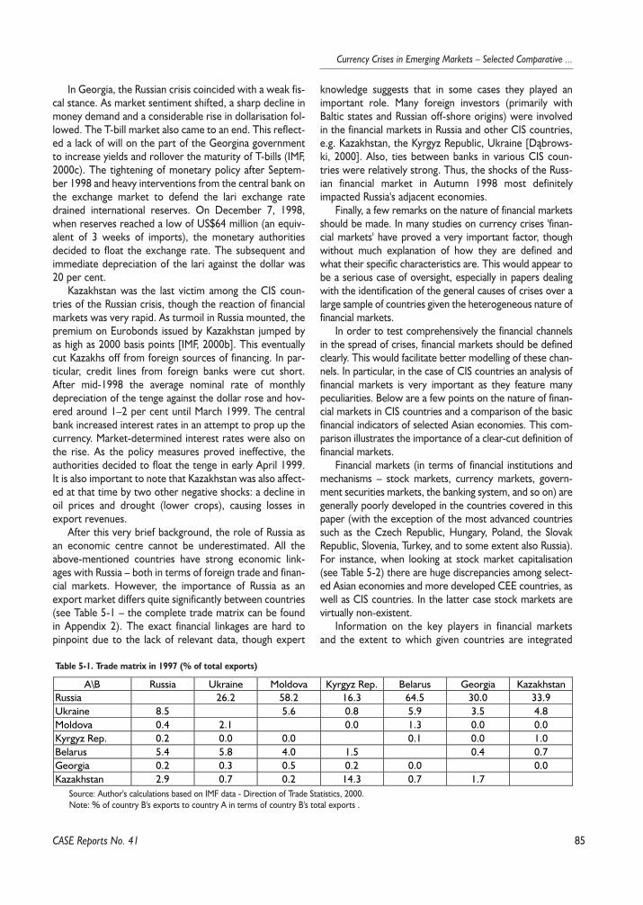
85
Currency Crises in Emerging Markets – Selected Comparative ...
In Georgia, the Russian crisis coincided with a weak fis-cal stance. As market sentiment shifted, a sharp decline inmoney demand and a considerable rise in dollarisation fol-lowed. The T-bill market also came to an end. This reflect-ed a lack of will on the part of the Georgina governmentto increase yields and rollover the maturity of T-bills (IMF,2000c). The tightening of monetary policy after Septem-ber 1998 and heavy interventions from the central bank onthe exchange market to defend the lari exchange ratedrained international reserves. On December 7, 1998,when reserves reached a low of US$64 million (an equiv-alent of 3 weeks of imports), the monetary authoritiesdecided to float the exchange rate. The subsequent andimmediate depreciation of the lari against the dollar was20 per cent.
Kazakhstan was the last victim among the CIS coun-tries of the Russian crisis, though the reaction of financialmarkets was very rapid. As turmoil in Russia mounted, thepremium on Eurobonds issued by Kazakhstan jumped byas high as 2000 basis points [IMF, 2000b]. This eventuallycut Kazakhs off from foreign sources of financing. In par-ticular, credit lines from foreign banks were cut short.After mid-1998 the average nominal rate of monthlydepreciation of the tenge against the dollar rose and hov-ered around 1–2 per cent until March 1999. The centralbank increased interest rates in an attempt to prop up thecurrency. Market-determined interest rates were also onthe rise. As the policy measures proved ineffective, theauthorities decided to float the tenge in early April 1999.It is also important to note that Kazakhstan was also affect-ed at that time by two other negative shocks: a decline inoil prices and drought (lower crops), causing losses inexport revenues.
After this very brief background, the role of Russia asan economic centre cannot be underestimated. All theabove-mentioned countries have strong economic link-ages with Russia – both in terms of foreign trade and finan-cial markets. However, the importance of Russia as anexport market differs quite significantly between countries(see Table 5-1 – the complete trade matrix can be foundin Appendix 2). The exact financial linkages are hard topinpoint due to the lack of relevant data, though expert
knowledge suggests that in some cases they played animportant role. Many foreign investors (primarily withBaltic states and Russian off-shore origins) were involvedin the financial markets in Russia and other CIS countries,e.g. Kazakhstan, the Kyrgyz Republic, Ukraine [D¹brows-ki, 2000]. Also, ties between banks in various CIS coun-tries were relatively strong. Thus, the shocks of the Russ-ian financial market in Autumn 1998 most definitelyimpacted Russia's adjacent economies.
Finally, a few remarks on the nature of financial marketsshould be made. In many studies on currency crises 'finan-cial markets' have proved a very important factor, thoughwithout much explanation of how they are defined andwhat their specific characteristics are. This would appear tobe a serious case of oversight, especially in papers dealingwith the identification of the general causes of crises over alarge sample of countries given the heterogeneous nature offinancial markets.
In order to test comprehensively the financial channelsin the spread of crises, financial markets should be definedclearly. This would facilitate better modelling of these chan-nels. In particular, in the case of CIS countries an analysis offinancial markets is very important as they feature manypeculiarities. Below are a few points on the nature of finan-cial markets in CIS countries and a comparison of the basicfinancial indicators of selected Asian economies. This com-parison illustrates the importance of a clear-cut definition offinancial markets.
Financial markets (in terms of financial institutions andmechanisms – stock markets, currency markets, govern-ment securities markets, the banking system, and so on) aregenerally poorly developed in the countries covered in thispaper (with the exception of the most advanced countriessuch as the Czech Republic, Hungary, Poland, the SlovakRepublic, Slovenia, Turkey, and to some extent also Russia).For instance, when looking at stock market capitalisation(see Table 5-2) there are huge discrepancies among select-ed Asian economies and more developed CEE countries, aswell as CIS countries. In the latter case stock markets arevirtually non-existent.
Information on the key players in financial marketsand the extent to which given countries are integrated
CASE Reports No. 41
Table 5-1. Trade matrix in 1997 (% of total exports)
A\B Russia Ukraine Moldova Kyrgyz Rep. Belarus Georgia KazakhstanRussia 26.2 58.2 16.3 64.5 30.0 33.9Ukraine 8.5 5.6 0.8 5.9 3.5 4.8Moldova 0.4 2.1 0.0 1.3 0.0 0.0Kyrgyz Rep. 0.2 0.0 0.0 0.1 0.0 1.0Belarus 5.4 5.8 4.0 1.5 0.4 0.7Georgia 0.2 0.3 0.5 0.2 0.0 0.0Kazakhstan 2.9 0.7 0.2 14.3 0.7 1.7
Source: Author's calculations based on IMF data - Direction of Trade Statistics, 2000.Note: % of country B's exports to country A in terms of country B's total exports .
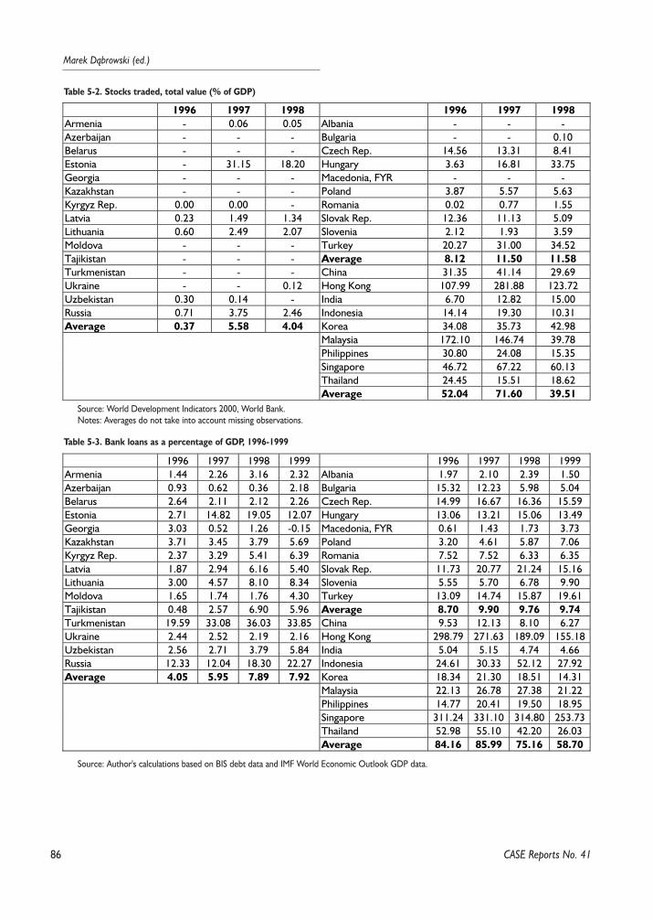
86
Marek D¹browski (ed.)
CASE Reports No. 41
Table 5-2. Stocks traded, total value (% of GDP)
1996 1997 1998 1996 1997 1998Armenia - 0.06 0.05 Albania - - -Azerbaijan - - - Bulgaria - - 0.10Belarus - - - Czech Rep. 14.56 13.31 8.41Estonia - 31.15 18.20 Hungary 3.63 16.81 33.75Georgia - - - Macedonia, FYR - - -Kazakhstan - - - Poland 3.87 5.57 5.63Kyrgyz Rep. 0.00 0.00 - Romania 0.02 0.77 1.55Latvia 0.23 1.49 1.34 Slovak Rep. 12.36 11.13 5.09Lithuania 0.60 2.49 2.07 Slovenia 2.12 1.93 3.59Moldova - - - Turkey 20.27 31.00 34.52Tajikistan - - - Average 8.12 11.50 11.58Turkmenistan - - - China 31.35 41.14 29.69Ukraine - - 0.12 Hong Kong 107.99 281.88 123.72Uzbekistan 0.30 0.14 - India 6.70 12.82 15.00Russia 0.71 3.75 2.46 Indonesia 14.14 19.30 10.31Average 0.37 5.58 4.04 Korea 34.08 35.73 42.98
Malaysia 172.10 146.74 39.78Philippines 30.80 24.08 15.35Singapore 46.72 67.22 60.13Thailand 24.45 15.51 18.62Average 52.04 71.60 39.51
Source: World Development Indicators 2000, World Bank.Notes: Averages do not take into account missing observations.
Table 5-3. Bank loans as a percentage of GDP, 1996-1999
1996 1997 1998 1999 1996 1997 1998 1999Armenia 1.44 2.26 3.16 2.32 Albania 1.97 2.10 2.39 1.50Azerbaijan 0.93 0.62 0.36 2.18 Bulgaria 15.32 12.23 5.98 5.04Belarus 2.64 2.11 2.12 2.26 Czech Rep. 14.99 16.67 16.36 15.59Estonia 2.71 14.82 19.05 12.07 Hungary 13.06 13.21 15.06 13.49Georgia 3.03 0.52 1.26 -0.15 Macedonia, FYR 0.61 1.43 1.73 3.73Kazakhstan 3.71 3.45 3.79 5.69 Poland 3.20 4.61 5.87 7.06Kyrgyz Rep. 2.37 3.29 5.41 6.39 Romania 7.52 7.52 6.33 6.35Latvia 1.87 2.94 6.16 5.40 Slovak Rep. 11.73 20.77 21.24 15.16Lithuania 3.00 4.57 8.10 8.34 Slovenia 5.55 5.70 6.78 9.90Moldova 1.65 1.74 1.76 4.30 Turkey 13.09 14.74 15.87 19.61Tajikistan 0.48 2.57 6.90 5.96 Average 8.70 9.90 9.76 9.74Turkmenistan 19.59 33.08 36.03 33.85 China 9.53 12.13 8.10 6.27Ukraine 2.44 2.52 2.19 2.16 Hong Kong 298.79 271.63 189.09 155.18Uzbekistan 2.56 2.71 3.79 5.84 India 5.04 5.15 4.74 4.66Russia 12.33 12.04 18.30 22.27 Indonesia 24.61 30.33 52.12 27.92Average 4.05 5.95 7.89 7.92 Korea 18.34 21.30 18.51 14.31
Malaysia 22.13 26.78 27.38 21.22Philippines 14.77 20.41 19.50 18.95Singapore 311.24 331.10 314.80 253.73Thailand 52.98 55.10 42.20 26.03Average 84.16 85.99 75.16 58.70
Source: Author's calculations based on BIS debt data and IMF World Economic Outlook GDP data.
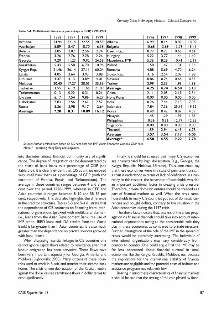
87
Currency Crises in Emerging Markets – Selected Comparative ...
into the international financial community are of signifi-cance. The degree of integration can be demonstrated bythe share of bank loans as a percentage of GDP (seeTable 5-3). It is clearly evident that CIS countries enjoyedvery small bank loans as a percentage of GDP (with theexception of Estonia, Russia, and Turkmenistan). Theaverage in these countries ranges between 4 and 8 percent over the period 1996–1999, whereas in CEE andAsian countries it ranges between 8–10 and 58–86 percent, respectively. This data also highlights the differencein the creditor structure. Tables 5-3 and 5-4 illustrate thatthe dependence of CIS countries on financing from inter-national organisations (proxied with multilateral claims –i.e., loans from the Asian Development Bank, the use ofIMF credit, IBRD loans and IDA credits from the WorldBank) is far greater than in Asian countries. It is also muchgreater than the dependence on private sources (proxiedwith bank loans).
When discussing financial linkages in CIS countries onecannot ignore capital flows related to remittance given thatlabour emigration has been pervasive. These flows havebeen very important especially for Georgia, Armenia, andMoldova (D¹browski, 2000). Many citizens of these coun-tries used to work in Russia and transfer their income backhome. The crisis-driven depreciation of the Russian roubleagainst the dollar caused remittance flows in dollar terms todrop significantly.
Finally, it should be stressed that many CIS economiesare characterised by high dollarisation (e.g., Georgia, theKyrgyz Republic, Moldova, Ukraine). Thus, one could saythat these economies were in a state of permanent crisis, ifa crisis is understood in terms of lack of confidence in a cur-rency. In this respect, the behaviour of households was alsoan important additional factor in creating crisis pressure.Therefore, private domestic entities should be treaded as apart of financial markets as well. When the crisis came,households in many CIS countries got out of domestic cur-rencies and bought dollars, contrary to the situation in theAsian economies during the 1997 crisis.
The above facts indicate that, analysis of the crises prop-agation via financial channels should take into account inter-national organisations owing to the considerable role theyplay in these economies as compared to private investors.Further investigation of the role of the IMF in the spread ofcrises would be extremely interesting. The behaviour ofinternational organisations may vary considerably fromcountry to country. One could argue that the IMF may befar less concerned about financial turmoil in smalleconomies like the Kyrgyz Republic, Moldova, etc. becausethe implications for the international stability of financialmarkets are negligible and the potential costs of bailouts andassistance programmes relatively low.
Bearing in mind these characteristics of financial marketsit should be said that the testing of the role played by finan-
CASE Reports No. 41
Table 5-4. Multilateral claims as a percentage of GDP, 1996-1999
1996 1997 1998 1999 1996 1997 1998 1999Armenia 14.94 22.14 22.54 28.59 Albania 6.99 8.14 8.89 10.09Azerbaijan 5.89 8.47 10.70 16.38 Bulgaria 10.68 13.69 13.76 15.41Belarus 2.85 2.82 2.56 2.74 Czech Rep. 0.77 0.73 0.65 0.61Estonia 3.26 2.76 2.28 2.26 Hungary 5.22 3.77 1.44 1.40Georgia 9.29 11.23 19.92 24.58 Macedonia, FYR 5.36 8.28 10.41 12.11Kazakhstan 5.43 5.58 6.70 10.96 Poland 1.58 1.47 1.31 1.36Kyrgyz Rep. 21.46 26.14 37.11 60.04 Romania 4.88 5.69 4.70 6.24Latvia 4.05 3.64 3.93 3.88 Slovak Rep. 3.16 2.54 2.07 1.88Lithuania 4.37 4.13 3.89 4.01 Slovenia 0.86 0.74 0.65 0.53Moldova 20.40 17.27 20.05 35.53 Turkey 2.99 2.33 1.91 1.68Tajikistan 3.55 6.19 11.65 21.09 Average 4.25 4.74 4.58 5.13Turkmenistan 0.13 0.22 0.31 0.21 China 2.11 2.05 2.19 2.34Ukraine 6.17 7.54 9.86 16.27 Hong Kong 0.00 0.00 0.00 0.00Uzbekistan 2.83 2.56 2.61 2.57 India 8.26 7.44 7.13 7.05Russia 3.36 3.98 9.17 12.64 Indonesia 7.84 7.36 25.18 19.32Average 7.20 8.31 10.89 16.12 Korea 0.49 0.42 8.87 4.59
Malaysia 1.45 1.29 1.99 1.83Philippines 10.36 10.36 12.77 12.55Singapore 0.00 0.00 0.00 0.00Thailand 1.59 2.94 6.43 6.78Average 3.57 3.54 7.17 6.05Average* 4.58 4.55 9.22 7.78
Source: Author's calculations based on BIS debt data and IMF World Economic Outlook GDP data. Note: * - excluding Hong Kong and Singapore.

88
Marek D¹browski (ed.)
cial channels in CIS countries is more difficult than is the casein developed markets. Theoretically, it would be easier toidentify the reaction function of investors if there were nodistortions in the markets. This is definitely not the case forCIS countries as multiple (Belarus and Uzbekistan) or dou-ble exchange rate systems (Turkmenistan) and restrictionson foreign currency transactions (Belarus) exist. In addition,the availability and reliability of financial data is far worsethan in developed countries. On the other hand, the multi-plicity of financial instruments in developed economies doesnot make the analysis easier.
5.5.3. The Probit Model
In order to test the role of trade linkages (and, in turn,of spillovers) in the propagation of the Russian crisis we haveestimated a simple probit model. The crisis is defined with abinary variable (1 – crisis occurred, 0 no crisis occurred).Russia represents the ground-zero country. Of the 24 coun-tries in the sample (a detailed list is provided in Appendix 1),6 were identified as crisis-hit countries (Belarus, Georgia,Moldova, Kazakhstan, the Kyrgyz Republic, and Ukraine).Given the numerous problems with data availability and reli-ability the crisis variable is explained only with the use oftrade shares and a single macroeconomic variable.
The trade variable is constructed so as to indicate theimportance in any given crisis-hit country of export markets.This is the cumulative share of exports in their total exports.As such, this variable takes into account not only the ground-zero country, but also those countries that were infectedwith the crisis previously. For countries that did not experi-ence the crisis it is the cumulative share of exports to all cri-sis-hit countries. The shares are based on annual data from1997. 1998 was not chosen as the reference year as the con-siderable devaluations/deprecations that occurred in thisyear could bias the results. It was decided to incorporateonly the direct trade channel (see Section 5.3), as no detaileddata on the commodity structure of analysed countries wereavailable and it was thus impossible to make any inference interms of the competition effect in third markets or the bar-gaining effect.
The higher the share of exports to crisis-hit countries(i.e., countries that devalued/depreciated their currencies),the higher probability, ceteris paribus, of a trade balancedeterioration in the given country. As a consequence, thismay lead to a balance of payments crisis. Thus, the expect-ed sign of this variable in the model is positive. At this pointis should be stressed that trade statistics in CIS countries arewidely deemed to be erratic and thus should be treadedwith great caution. This problem stems primarily from'transparent' borders, low statistical coverage, discrepanciesdue to the translation into dollars and the large share ofbarter and shuttle trade.
Due to hard data constraints (both with regard to avail-ability and reliability) the macroeconomic variable coversonly the ratio of total reserves minus gold (as of the end ofthe third quarter of 1998) to exports (for 1998 as a whole,fob). The higher the ratio, the lower probability that ashock to the trade balance will cause balance of paymentsproblems (higher/lower trade deficit/surplus can be financedwith reserves). Therefore, this coefficient's sign should benegative.
A richer set of macroeconomic variables would seem tobe more instructive and an occurrence of the omitted vari-able error less probable. Unfortunately, the small samplesize made it impossible to estimate such a model. In variouspapers macroeconomic variables are added in order to con-trol for differences in these variables across countries. Forinstance, Glick and Rose (1999) inserted credit growth, bud-get balance to GDP, current account balance to GDP, GDPgrowth, M2 to reserves and inflation. However, as Pritsker(2000) noted, the inclusion of fundamentals is not the sameas controlling for them in an economic model. Properlycontrolling the role of fundamental is possible only when allthe ways in which the fundamentals can influence the eco-nomic situation are identified.
Prior to turning to the discussion of results, the problemof 'time inconsistency' in the variables of the above modelshould be brought to attention. The variables are measuredat different points in time, which is conceptually incorrect.On reason behind such a situation is the previously dis-cussed problem of defining the moments of crisis outbreakand elapse. The other handicap is the lack of high-frequen-cy data. For instance, in the case of this paper's country cov-erage debt data are only available on an annual basis withsome exceptions on a quarterly basis. The problem is evenmore profound when ratios are used. In this case variablesare usually not only measured in different points in time, butalso stock and flow variables are mixed. The long time-scaleof crisis spreading under the investigation here does notmake things easier, especially if it covers the turn of twoyears.
A potential solution to this problem could be theemployment of multiperiod multinomial discrete choice anddiscrete/continuous econometric specifications with flexiblecorrelation structures in unobservables as developed byHajivassiliou and McFadden (1990). They illustrated that theestimation of these models based on simulation methodshas attractive statistical properties and is computationallytractable. The models were applied to an analysis of exter-nal debt crises in developing countries.
The detailed results of the estimatesion are presented inAppendix 3. Below we outline only the probabilities of a cri-sis in a given country as computed in the model (see Table5-5). Given a cut-off point of 50 per cent, the model pre-dicted one crisis out of six and also two crises which did nothappen. The former case applies to the Kyrgyz Republic.
CASE Reports No. 41
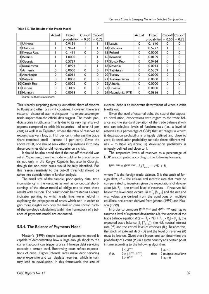
89
Currency Crises in Emerging Markets – Selected Comparative ...
This is hardly surprising given its low official share of exportsto Russia and other crisis-hit countries. However, there arereasons – discussed later in this paper – to expect a strongertrade impact than the official data suggest. The model pre-dicts a crisis in Lithuania (mainly due to its very high share ofexports compared to crisis-hit countries – of over 45 percent) as well as in Tajikistan, where the ratio of reserves toexports was very low, at 11.1 per cent (whereas the tradeshare remained small – around 11 per cent). Given theabove result, one should seek other explanations as to whythese countries did or did not experience a crisis.
It should be also noted that if the cut-off threshold wasset at 75 per cent, then the model would fail to predict a cri-sis not only in the Kyrgyz Republic but also in Georgia,though the non-crisis cases would be fully identified. Forthis reason sensitivity to the cut-off threshold should betaken into consideration in further analysis.
The small size of the sample, poor quality data, timeinconsistency in the variables as well as conceptual short-comings of the above model all oblige one to treat theseresults with caution. The result should be treated as a roughindicator pointing to which trade links were helpful inexplaining the propagation of crises which not. In order togain more insights into how the Russian crisis spread back-of-the-envelope calculations within the framework of a bal-ance of payments model are conducted.
5.5.4. The Balance of Payments Model
Masson's (1999) simple balance of payments model iscapable of demonstrating how a large enough shock to thecurrent account can trigger a crisis if foreign debt servicingexceeds a certain level. Borrowing costs reflect expecta-tions of crisis. Higher interest rates make debt servicingmore expensive and can deplete reserves, which in turnmay lead to devaluation. In this framework, the size of
external debt is an important determinant of when a crisisbreaks out.
Given the level of external debt, the size of the expect-ed devaluation, expectations with regard to the trade bal-ance and the standard deviation of the trade balance shockone can calculate levels of fundamentals (i.e., a level ofreserves as a percentage of GDP) that set ranges in which:i) devaluation probability is uniquely defined and close tozero; ii) devaluation probability can take three different val-ues – multiple equilibria; iii) devaluation probability isuniquely defined and close to 1.
The respective levels of reserves as a percentage ofGDP are computed according to the following formula:
Rmin, max ≡ Φmin, max - Et(Tt+1) + r*D + Rc,
where T is the foreign trade balance, D is the stock of for-eign debt, r* – the risk-neutral interest rate that must becompensated to investors given the expectations of devalu-ation (δ), Rc – the critical level of reserves – if reserves fallbelow this level crisis occurs. Φ ≡ Et [bt+1] and the min andmax values are derived from the conditions on multipleequilibria occurrence derived from Jeanne (1997) and Mas-son (1999).
In order to compute Rmin, max and Φmin, max one has toassume a level of expected devaluation (δ), the variance of thetrade balance equation σ (ε = [Tt - r*D + Rt-1 - Rc] - Φt-1), theexpected trade balance (Et [Tt+1]), the risk-neutral interestrate (r*) and the critical level of reserves (Rc). Besides this,the stock of external debt (D) and the level of reserves (R)must be known. Given these inputs one can determine theprobability of a crisis (πt) in a given country at a certain pointin time according to the following algorithm:
if
CASE Reports No. 41
Table 5-5. The Results of the Probit Model
Actual Fittedprobability
Cut-off= 0.50
Cut-off= 0.75
Actual Fittedprobability
Cut-off= 0.50
Cut-off= 0.75
1 Ukraine 1 0.9154 1 1 13 Latvia 0 0.1640 0 02 Moldova 1 0.9474 1 1 14 Lithuania 0 0.5277 1 03 Kyrgyz Rep. 1 0.1411 0 0 15 Poland 0 0.0000 0 04 Belarus 1 1.0000 1 1 16 Romania 0 0.0109 0 05 Georgia 1 0.5739 1 0 17 Slovak Rep. 0 0.0424 0 06 Kazakhstan 1 0.8924 1 1 18 Slovenia 0 0.0013 0 07 Armenia 0 0.0000 0 0 19 Tajikistan 0 0.5309 1 08 Azerbaijan 0 0.0011 0 0 20 Turkey 0 0.0000 0 09 Bulgaria 0 0.0000 0 0 21 Turkmenistan 0 0.0000 0 0
10 Czech Rep. 0 0.0002 0 0 22 Albania 0 0.0000 0 011 Estonia 0 0.3009 0 0 23 Croatia 0 0.0000 0 012 Hungary 0 0.0018 0 0 24 Macedonia, FYR 0 0.0656 0 0
Source: Author's calculations.
< Rmin πt ≈ 1Rt ∈ [Rmin, Rmax] then multiple equilibria
> Rmax πt ≈ 0
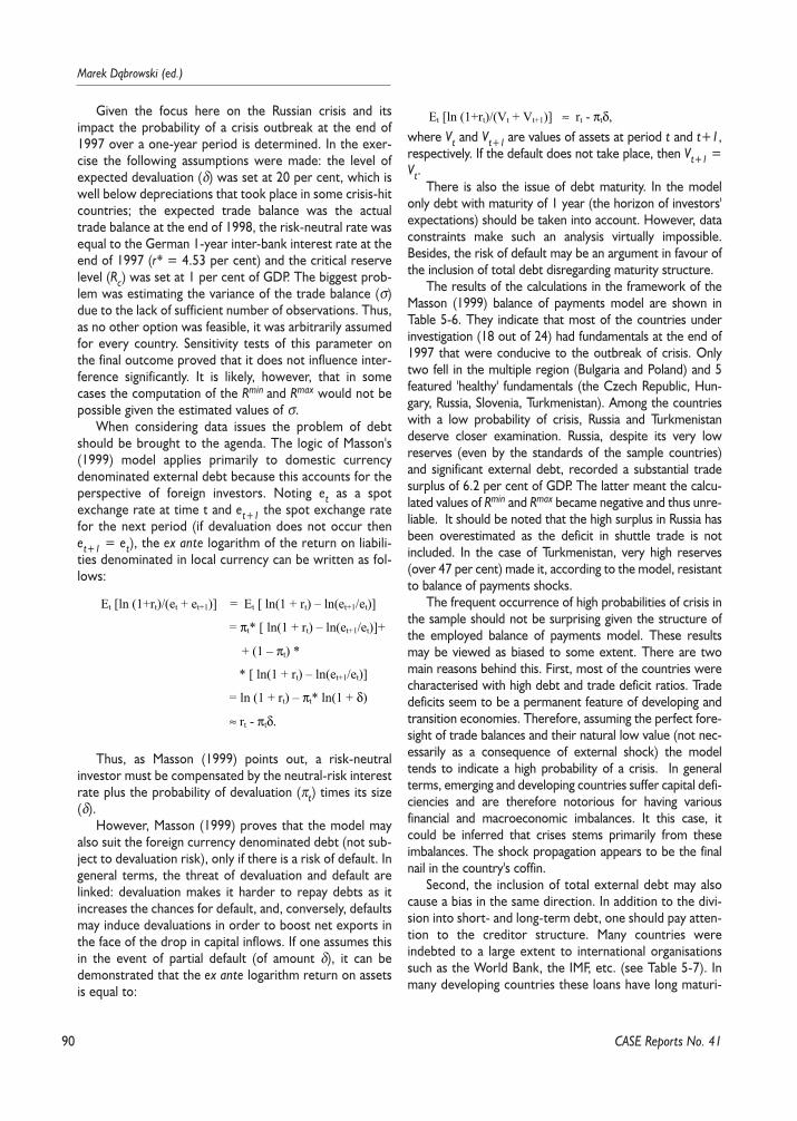
90
Marek D¹browski (ed.)
Given the focus here on the Russian crisis and itsimpact the probability of a crisis outbreak at the end of1997 over a one-year period is determined. In the exer-cise the following assumptions were made: the level ofexpected devaluation (δ) was set at 20 per cent, which iswell below depreciations that took place in some crisis-hitcountries; the expected trade balance was the actualtrade balance at the end of 1998, the risk-neutral rate wasequal to the German 1-year inter-bank interest rate at theend of 1997 (r* = 4.53 per cent) and the critical reservelevel (Rc) was set at 1 per cent of GDP. The biggest prob-lem was estimating the variance of the trade balance (σ)due to the lack of sufficient number of observations. Thus,as no other option was feasible, it was arbitrarily assumedfor every country. Sensitivity tests of this parameter onthe final outcome proved that it does not influence inter-ference significantly. It is likely, however, that in somecases the computation of the Rmin and Rmax would not bepossible given the estimated values of σ.
When considering data issues the problem of debtshould be brought to the agenda. The logic of Masson's(1999) model applies primarily to domestic currencydenominated external debt because this accounts for theperspective of foreign investors. Noting et as a spotexchange rate at time t and et+1 the spot exchange ratefor the next period (if devaluation does not occur thenet+1 = et), the ex ante logarithm of the return on liabili-ties denominated in local currency can be written as fol-lows:
Thus, as Masson (1999) points out, a risk-neutralinvestor must be compensated by the neutral-risk interestrate plus the probability of devaluation (πt) times its size(δ).
However, Masson (1999) proves that the model mayalso suit the foreign currency denominated debt (not sub-ject to devaluation risk), only if there is a risk of default. Ingeneral terms, the threat of devaluation and default arelinked: devaluation makes it harder to repay debts as itincreases the chances for default, and, conversely, defaultsmay induce devaluations in order to boost net exports inthe face of the drop in capital inflows. If one assumes thisin the event of partial default (of amount δ), it can bedemonstrated that the ex ante logarithm return on assetsis equal to:
where Vt and Vt+1 are values of assets at period t and t+1,respectively. If the default does not take place, then Vt+1 =Vt.
There is also the issue of debt maturity. In the modelonly debt with maturity of 1 year (the horizon of investors'expectations) should be taken into account. However, dataconstraints make such an analysis virtually impossible.Besides, the risk of default may be an argument in favour ofthe inclusion of total debt disregarding maturity structure.
The results of the calculations in the framework of theMasson (1999) balance of payments model are shown inTable 5-6. They indicate that most of the countries underinvestigation (18 out of 24) had fundamentals at the end of1997 that were conducive to the outbreak of crisis. Onlytwo fell in the multiple region (Bulgaria and Poland) and 5featured 'healthy' fundamentals (the Czech Republic, Hun-gary, Russia, Slovenia, Turkmenistan). Among the countrieswith a low probability of crisis, Russia and Turkmenistandeserve closer examination. Russia, despite its very lowreserves (even by the standards of the sample countries)and significant external debt, recorded a substantial tradesurplus of 6.2 per cent of GDP. The latter meant the calcu-lated values of Rmin and Rmax became negative and thus unre-liable. It should be noted that the high surplus in Russia hasbeen overestimated as the deficit in shuttle trade is notincluded. In the case of Turkmenistan, very high reserves(over 47 per cent) made it, according to the model, resistantto balance of payments shocks.
The frequent occurrence of high probabilities of crisis inthe sample should not be surprising given the structure ofthe employed balance of payments model. These resultsmay be viewed as biased to some extent. There are twomain reasons behind this. First, most of the countries werecharacterised with high debt and trade deficit ratios. Tradedeficits seem to be a permanent feature of developing andtransition economies. Therefore, assuming the perfect fore-sight of trade balances and their natural low value (not nec-essarily as a consequence of external shock) the modeltends to indicate a high probability of a crisis. In generalterms, emerging and developing countries suffer capital defi-ciencies and are therefore notorious for having variousfinancial and macroeconomic imbalances. It this case, itcould be inferred that crises stems primarily from theseimbalances. The shock propagation appears to be the finalnail in the country's coffin.
Second, the inclusion of total external debt may alsocause a bias in the same direction. In addition to the divi-sion into short- and long-term debt, one should pay atten-tion to the creditor structure. Many countries wereindebted to a large extent to international organisationssuch as the World Bank, the IMF, etc. (see Table 5-7). Inmany developing countries these loans have long maturi-
CASE Reports No. 41
Et [ln (1+rt)/(et + et+1)] = Et [ ln(1 + rt) – ln(et+1/et)]
= πt* [ ln(1 + rt) – ln(et+1/et)]+
+ (1 – πt) *
* [ ln(1 + rt) – ln(et+1/et)]
= ln (1 + rt) – πt* ln(1 + δ)
≈ rt - πtδ.
Et [ln (1+rt)/(Vt + Vt+1)] ≈ rt - πtδ,
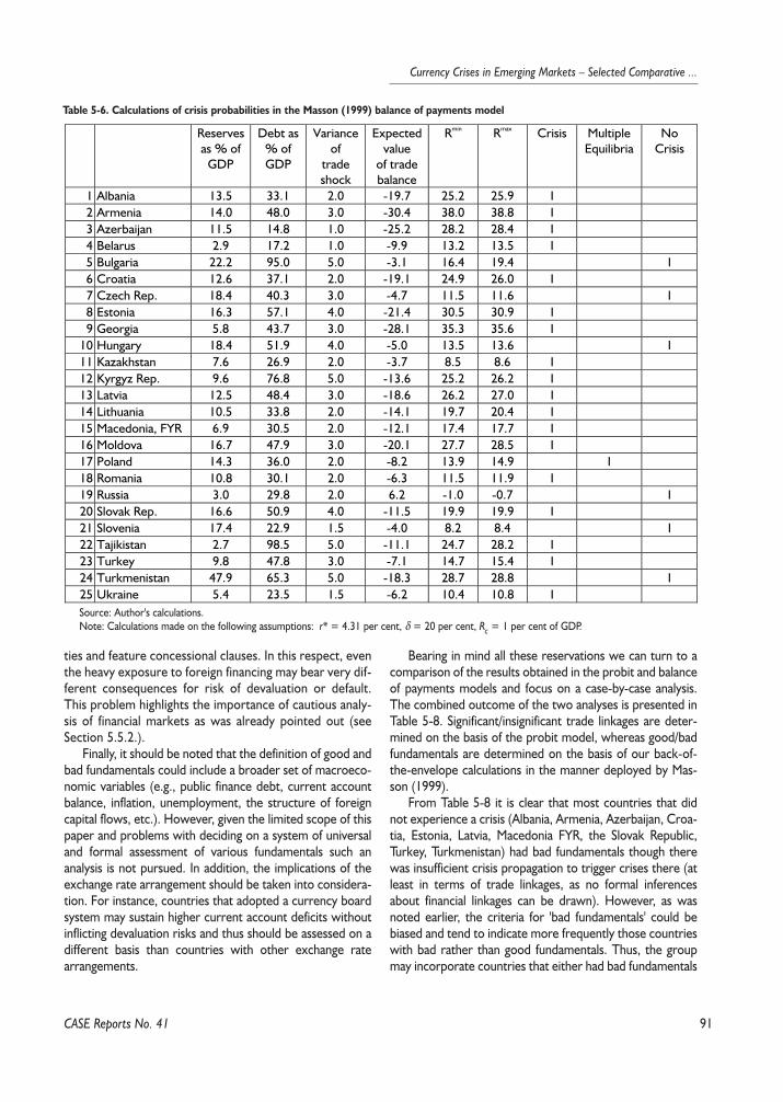
91
Currency Crises in Emerging Markets – Selected Comparative ...
ties and feature concessional clauses. In this respect, eventhe heavy exposure to foreign financing may bear very dif-ferent consequences for risk of devaluation or default.This problem highlights the importance of cautious analy-sis of financial markets as was already pointed out (seeSection 5.5.2.).
Finally, it should be noted that the definition of good andbad fundamentals could include a broader set of macroeco-nomic variables (e.g., public finance debt, current accountbalance, inflation, unemployment, the structure of foreigncapital flows, etc.). However, given the limited scope of thispaper and problems with deciding on a system of universaland formal assessment of various fundamentals such ananalysis is not pursued. In addition, the implications of theexchange rate arrangement should be taken into considera-tion. For instance, countries that adopted a currency boardsystem may sustain higher current account deficits withoutinflicting devaluation risks and thus should be assessed on adifferent basis than countries with other exchange ratearrangements.
Bearing in mind all these reservations we can turn to acomparison of the results obtained in the probit and balanceof payments models and focus on a case-by-case analysis.The combined outcome of the two analyses is presented inTable 5-8. Significant/insignificant trade linkages are deter-mined on the basis of the probit model, whereas good/badfundamentals are determined on the basis of our back-of-the-envelope calculations in the manner deployed by Mas-son (1999).
From Table 5-8 it is clear that most countries that didnot experience a crisis (Albania, Armenia, Azerbaijan, Croa-tia, Estonia, Latvia, Macedonia FYR, the Slovak Republic,Turkey, Turkmenistan) had bad fundamentals though therewas insufficient crisis propagation to trigger crises there (atleast in terms of trade linkages, as no formal inferencesabout financial linkages can be drawn). However, as wasnoted earlier, the criteria for 'bad fundamentals' could bebiased and tend to indicate more frequently those countrieswith bad rather than good fundamentals. Thus, the groupmay incorporate countries that either had bad fundamentals
CASE Reports No. 41
Table 5-6. Calculations of crisis probabilities in the Masson (1999) balance of payments model
Reservesas % of
GDP
Debt as% ofGDP
Varianceof
tradeshock
Expectedvalue
of tradebalance
Rmin Rmax Crisis MultipleEquilibria
NoCrisis
1 Albania 13.5 33.1 2.0 -19.7 25.2 25.9 12 Armenia 14.0 48.0 3.0 -30.4 38.0 38.8 13 Azerbaijan 11.5 14.8 1.0 -25.2 28.2 28.4 14 Belarus 2.9 17.2 1.0 -9.9 13.2 13.5 15 Bulgaria 22.2 95.0 5.0 -3.1 16.4 19.4 16 Croatia 12.6 37.1 2.0 -19.1 24.9 26.0 17 Czech Rep. 18.4 40.3 3.0 -4.7 11.5 11.6 18 Estonia 16.3 57.1 4.0 -21.4 30.5 30.9 19 Georgia 5.8 43.7 3.0 -28.1 35.3 35.6 1
10 Hungary 18.4 51.9 4.0 -5.0 13.5 13.6 111 Kazakhstan 7.6 26.9 2.0 -3.7 8.5 8.6 112 Kyrgyz Rep. 9.6 76.8 5.0 -13.6 25.2 26.2 113 Latvia 12.5 48.4 3.0 -18.6 26.2 27.0 114 Lithuania 10.5 33.8 2.0 -14.1 19.7 20.4 115 Macedonia, FYR 6.9 30.5 2.0 -12.1 17.4 17.7 116 Moldova 16.7 47.9 3.0 -20.1 27.7 28.5 117 Poland 14.3 36.0 2.0 -8.2 13.9 14.9 118 Romania 10.8 30.1 2.0 -6.3 11.5 11.9 119 Russia 3.0 29.8 2.0 6.2 -1.0 -0.7 120 Slovak Rep. 16.6 50.9 4.0 -11.5 19.9 19.9 121 Slovenia 17.4 22.9 1.5 -4.0 8.2 8.4 122 Tajikistan 2.7 98.5 5.0 -11.1 24.7 28.2 123 Turkey 9.8 47.8 3.0 -7.1 14.7 15.4 124 Turkmenistan 47.9 65.3 5.0 -18.3 28.7 28.8 125 Ukraine 5.4 23.5 1.5 -6.2 10.4 10.8 1Source: Author's calculations.Note: Calculations made on the following assumptions: r* = 4.31 per cent, δ = 20 per cent, Rc = 1 per cent of GDP.
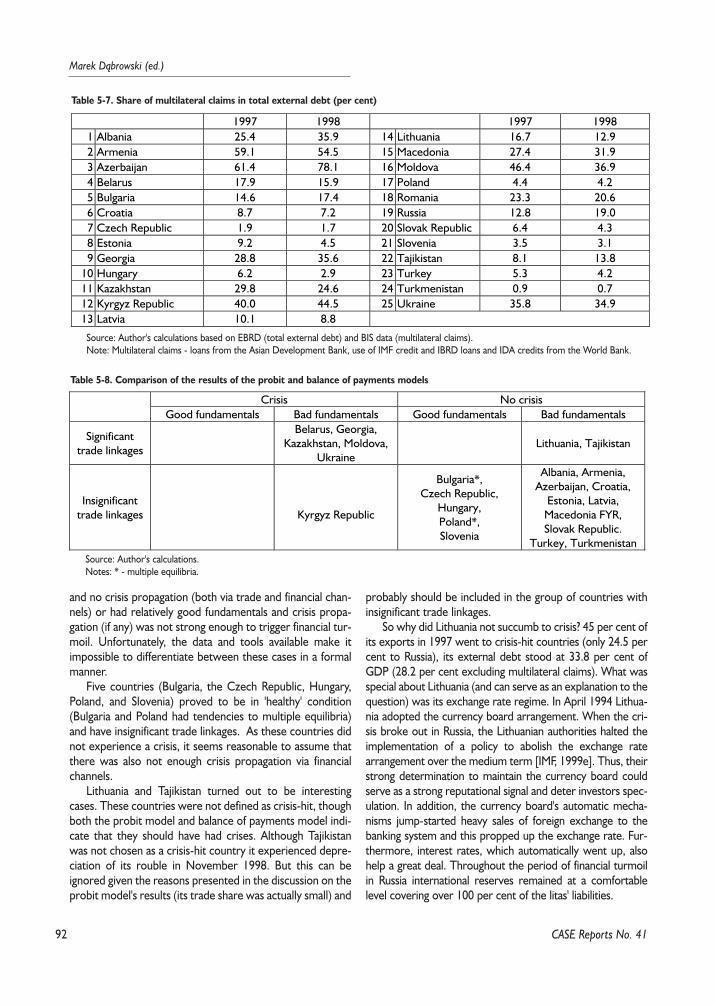
92
Marek D¹browski (ed.)
and no crisis propagation (both via trade and financial chan-nels) or had relatively good fundamentals and crisis propa-gation (if any) was not strong enough to trigger financial tur-moil. Unfortunately, the data and tools available make itimpossible to differentiate between these cases in a formalmanner.
Five countries (Bulgaria, the Czech Republic, Hungary,Poland, and Slovenia) proved to be in 'healthy' condition(Bulgaria and Poland had tendencies to multiple equilibria)and have insignificant trade linkages. As these countries didnot experience a crisis, it seems reasonable to assume thatthere was also not enough crisis propagation via financialchannels.
Lithuania and Tajikistan turned out to be interestingcases. These countries were not defined as crisis-hit, thoughboth the probit model and balance of payments model indi-cate that they should have had crises. Although Tajikistanwas not chosen as a crisis-hit country it experienced depre-ciation of its rouble in November 1998. But this can beignored given the reasons presented in the discussion on theprobit model's results (its trade share was actually small) and
probably should be included in the group of countries withinsignificant trade linkages.
So why did Lithuania not succumb to crisis? 45 per cent ofits exports in 1997 went to crisis-hit countries (only 24.5 percent to Russia), its external debt stood at 33.8 per cent ofGDP (28.2 per cent excluding multilateral claims). What wasspecial about Lithuania (and can serve as an explanation to thequestion) was its exchange rate regime. In April 1994 Lithua-nia adopted the currency board arrangement. When the cri-sis broke out in Russia, the Lithuanian authorities halted theimplementation of a policy to abolish the exchange ratearrangement over the medium term [IMF, 1999e]. Thus, theirstrong determination to maintain the currency board couldserve as a strong reputational signal and deter investors spec-ulation. In addition, the currency board's automatic mecha-nisms jump-started heavy sales of foreign exchange to thebanking system and this propped up the exchange rate. Fur-thermore, interest rates, which automatically went up, alsohelp a great deal. Throughout the period of financial turmoilin Russia international reserves remained at a comfortablelevel covering over 100 per cent of the litas' liabilities.
CASE Reports No. 41
Table 5-7. Share of multilateral claims in total external debt (per cent)
1997 1998 1997 19981 Albania 25.4 35.9 14 Lithuania 16.7 12.92 Armenia 59.1 54.5 15 Macedonia 27.4 31.93 Azerbaijan 61.4 78.1 16 Moldova 46.4 36.94 Belarus 17.9 15.9 17 Poland 4.4 4.25 Bulgaria 14.6 17.4 18 Romania 23.3 20.66 Croatia 8.7 7.2 19 Russia 12.8 19.07 Czech Republic 1.9 1.7 20 Slovak Republic 6.4 4.38 Estonia 9.2 4.5 21 Slovenia 3.5 3.19 Georgia 28.8 35.6 22 Tajikistan 8.1 13.8
10 Hungary 6.2 2.9 23 Turkey 5.3 4.211 Kazakhstan 29.8 24.6 24 Turkmenistan 0.9 0.712 Kyrgyz Republic 40.0 44.5 25 Ukraine 35.8 34.913 Latvia 10.1 8.8
Source: Author's calculations based on EBRD (total external debt) and BIS data (multilateral claims).Note: Multilateral claims - loans from the Asian Development Bank, use of IMF credit and IBRD loans and IDA credits from the World Bank.
Table 5-8. Comparison of the results of the probit and balance of payments models
Crisis No crisisGood fundamentals Bad fundamentals Good fundamentals Bad fundamentals
Significanttrade linkages
Belarus, Georgia,Kazakhstan, Moldova,
UkraineLithuania, Tajikistan
Insignificanttrade linkages Kyrgyz Republic
Bulgaria*,Czech Republic,
Hungary,Poland*,Slovenia
Albania, Armenia,Azerbaijan, Croatia,
Estonia, Latvia,Macedonia FYR,Slovak Republic.
Turkey, TurkmenistanSource: Author's calculations.Notes: * - multiple equilibria.
93
Currency Crises in Emerging Markets – Selected Comparative ...
CASE Reports No. 41
The second interesting case is the Kyrgyz Republic. Interms of official trade linkages one could have expectedthe country to avoid a currency crisis given its low share ofexports to crisis-hit countries. However, these figures maybe slightly misleading. IMF trade statistics do not includeshuttle trade. It is believed that such trade constitutes alarge share of official trade figures (both with respect toimports and exports). The geographic structure of shuttletrade should not differ significantly from registered tradeflows. Thus, in principle, the share of exports to crisis-hitcountries, in particularly to Russia, should be higher, ifaccounting for shuttle trade, and consequently, the trademodel should have been able to predict a crisis in the Kyr-gyz Republic. In addition, although external debt (excludingmultilateral claims) at over 40 per cent of GDP (seeAppendix 4) was not that high by regional standards, itseems that financial channels were the underlying cause ofthe propagation of the crisis. At the end of 1997, 18.7 percent of the country's external public debt was owed to CIScreditors on a non-concessional basis and this was roughlyat the level of international reserves excluding gold. Thus,the withdrawal of Russian and Kazakh creditors [IMF,1999c] could have impacted the market, especially in theface of a very shallow exchange rate market. Moreover, alack of confidence in the som was also expressed on thehousehold side – high dollarisation and low householdbanking deposits are a fact in the Kyrgyz Republic. Finally,it should be noted that external pressures in the aftermathof the Russian crisis coincided with other unfavourabledevelopments. Kyrgyz exports were hit by protectionisttrade measures introduced by Kazakhstan and Uzbekistan– important trading partners – and the drop in gold pricesin 1998. Gold comprises a significant share of official Kyr-gyz exports. These two factors definitely increased theodds of a crisis in the Kyrgyz Republic.
Summarising these results, one can say that all of the cri-sis-hit countries should be classified as having conditionsconducive to crisis and that the actual timing of crises wasdetermined by the shock propagation (both trade and finan-cial channels were important). These conducive conditionsdo not have to be defined only in terms of the balance ofpayments model, but also in terms of various macroeco-nomic imbalances that were present in many analysed coun-tries (for instance high current account and budget deficits).
It would be also interesting to know if any of the crisis-inflicted countries would have had a crisis regardless ofdevelopments in Russia. Unfortunately, there are no formaltools to assess such a possibility, though one could make anexpert guess based on the available information. Amongothers, Ukraine would have appeared to be such a country.As Markiewicz (2001) noted, Ukraine had been on theverge of crisis for some time prior to the financial turmoil inRussia and the later developments only hastened the melt-down. Also Moldova, the Kyrgyz Republic, Georgia and
Belarus, with profound fiscal imbalance problems, wereexposed to currency crisis risks.
In the case of countries that did not experience crisestwo groups are represented. The first comprises economiesthat proved to be immune to financial turmoil and trade-related spillovers. Financial linkages were insufficient tochange this. On the other hand, a second group was identi-fied as having bad fundamentals and thus prone to crises. Asthey did not actually suffer turmoil this tends to suggest thatthe propagation mechanisms were not present. However, itshould be stressed that the differentiation between 'healthy'and 'ill' countries is far from perfect.
On top of the above-mentioned channels by which crisiswere spread in the Russian case one should also note thepsychological factor suggested by D¹browski (2000) whichrefers in particular to FSU states. The legacy of former inte-gration and centralisation in the framework of the USSR'scommand economy inclined many politicians, economists aswell as ordinary people to think that economic develop-ments in Russian must follow the same path in other FSUstates. As such, in the aftermath of the Russian crisis therewere strong expectations of financial turmoil in other CIScountries. In some cases – the Kyrgyz Republic and Kaza-khstan – this proved a self-fulfilling prophecy.
5.6. Conclusions
The recent wave of currency crises in the 1980s and1990s has led to a resumption of studies on this economicphenomenon and, in particular, on the propagation of crisis.Despite the proliferation of studies and advancements intheory and empirical research, there are still some unclearaspects. One reason behind this is the problem of finding auniversal and formal definition of crisis as well as of conta-gion. Nonetheless, there is a consensus over the channels bywhich crisis spread. These are multiple equilibria, endoge-nous liquidity shock (or common bank lender), political con-tagion, trade, and common aggregate shocks. Empirical test-ing took one of two paths: testing if contagion was presentand testing what influences the propagation. The formergenerally used correlation-coefficient based models, whilethe latter used limited dependent variable models. Bothapproaches suffer from econometric problems of omittedvariables, heteroscedasticity, and endogeneity.
This paper claims that empirical research lags behind thedevelopment of contagion theory because of: problems ofcrisis definition, real world complexities, the mutual deter-mination of various channels that cannot be single out – forinstance interdependence of fundamentals and expectationsof financial markets and finally the impossibility of properlyincorporating financial markets. The latter stems primarily
94
Marek D¹browski (ed.)
from the heterogeneity of financial markets, probablyinstantaneous changes in parameters of their reaction func-tions and informational asymmetries.
Recognising these problems and data constraints (bothwith regard to availability and reliability) the paper analysesthe propagation of the Russian crisis among 24 CEE and CIScountries. The simple probit model and the balance of pay-ments model developed by Masson (1999) have beenemployed. The former identified the significance of tradelinks and the latter the stance of fundamentals in terms ofdebt exposure and susceptibility to trade balance shocks.Given their methodological and data deficiencies the resultshave been treated with caution. Thus, they were analysedagainst the background of stylised facts and specific featuresof financial markets in CIS countries.
The research proved that the propagation of crises tookplace mostly in countries with very bad fundamentals andstrong trade linkages to the ground-zero country – Russia.However, the linkages were not the whole story as in thecase of Lithuania the exchange rate regime acted as a suc-cessful defender against the crisis or, as in the case of theKyrgyz Republic, the small official trade exposure did notprevent financial factors from triggering a crisis.
Among countries not affected by crises many werefound to be in poor condition, though the crisis propagationwas not able to trigger financial turmoil due to a lack of sig-nificant trade and financial linkages.
CASE Reports No. 41
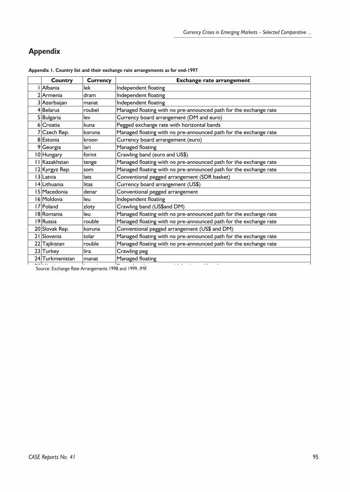
95
Currency Crises in Emerging Markets – Selected Comparative ...
Appendix
CASE Reports No. 41
Appendix 1. Country list and their exchange rate arrangements as for end-1997
Country Currency Exchange rate arrangement1 Albania lek Independent floating2 Armenia dram Independent floating3 Azerbaijan manat Independent floating4 Belarus roubel Managed floating with no pre-announced path for the exchange rate5 Bulgaria lev Currency board arrangement (DM and euro)6 Croatia kuna Pegged exchange rate with horizontal bands7 Czech Rep. koruna Managed floating with no pre-announced path for the exchange rate8 Estonia kroon Currency board arrangement (euro)9 Georgia lari Managed floating
10 Hungary forint Crawling band (euro and US$)11 Kazakhstan tenge Managed floating with no pre-announced path for the exchange rate12 Kyrgyz Rep. som Managed floating with no pre-announced path for the exchange rate13 Latvia lats Conventional pegged arrangement (SDR basket)14 Lithuania litas Currency board arrangement (US$)15 Macedonia denar Conventional pegged arrangement16 Moldova leu Independent floating17 Poland zloty Crawling band (US$and DM)18 Romania leu Managed floating with no pre-announced path for the exchange rate19 Russia rouble Managed floating with no pre-announced path for the exchange rate20 Slovak Rep. koruna Conventional pegged arrangement (US$ and DM)21 Slovenia tolar Managed floating with no pre-announced path for the exchange rate22 Tajikistan rouble Managed floating with no pre-announced path for the exchange rate23 Turkey lira Crawling peg24 Turkmenistan manat Managed floating25 Uk i h i P d h i h h i l b dSource: Exchange Rate Arrangements 1998 and 1999, IMF.
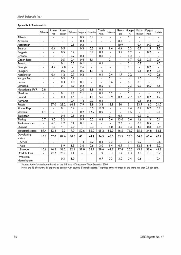
96
Marek D¹browski (ed.)
CASE Reports No. 41
Appendix 2. Trade matrix
AlbaniaArme-
niaAzer-baijan
Belarus Bulgaria CroatiaCzechRep.
EstoniaGeor-
giaHunga-
ryKaza-khstan
KyrgyzRep.
Latvia
Albania - - - 0.5 0.1 - - - 0.1 - - -Armenia - - - 0.3 - - - 8.3 - - - -Azerbaijan - - 0.1 0.3 - - - 10.9 - 0.4 0.5 0.1Belarus - 0.4 0.5 0.3 0.3 0.3 1.4 0.4 0.3 0.7 1.5 3.2Bulgaria - - 0.5 0.2 0.2 0.3 - 3.9 0.2 - 0.2 -Croatia - - - 0.2 0.3 0.8 - - 1.2 - - -Czech Rep. - - 0.5 0.4 0.4 1.1 0.1 - 1.7 0.3 2.5 0.4Estonia - - 0.1 0.2 0.1 - 0.1 - 0.1 0.7 - 4.2Georgia - 4.7 17.0 - 2.6 - - - 0.1 - 0.2 -Hungary - - 0.5 0.5 0.5 1.1 1.9 - - 0.1 0.2 0.1Kazakhstan - 0.4 1.2 0.7 0.2 - 0.1 0.4 1.7 0.2 14.3 0.6Kyrgyz Rep. - - 0.3 0.1 - - - 0.1 - - 1.0 0.1Latvia - - 0.3 1.0 0.1 - - 8.6 - 0.1 0.3 -Lithuania - - 0.1 1.9 0.2 - 0.5 6.1 - 0.3 0.7 0.5 7.5Macedonia, FYR 2.8 - - - 2.0 1.8 0.1 - - 0.1 - - -Moldova - - 0.1 1.3 2.1 - 0.1 0.2 - 0.1 - - 0.2Poland - - 0.4 3.4 - 1.1 5.6 0.9 0.4 2.7 0.4 0.2 1.2Romania - - - 0.4 1.4 0.3 0.4 - - - 0.1 0.2 -Russia - 27.0 23.2 64.5 7.9 3.8 3.3 18.8 30 5.1 33.9 16.3 21.0Slovak Rep. - - 0.1 0.4 - 0.5 12.9 - - 1.4 0.2 0.2 0.2Slovenia 1.4 - - - 0.2 12.2 0.9 - - 1.5 - - 0.1Tajikistan - - 0.4 0.1 0.4 - - 0.1 0.4 - 0.9 2.1 -Turkey 0.7 3.0 5.2 - 9.9 0.2 0.3 0.4 13.0 0.4 1.6 1.3 0.1Turkmenistan - 6.0 1.2 0.1 0.1 - - - 2.6 - 0.8 0.5 -Ukraine - 1.3 4.1 5.9 - 0.3 - 5.0 3.5 1.3 4.8 0.8 3.9Industrial states 89.4 32.2 12.3 9.0 50.6 55.0 65.2 55.0 16.5 76.7 35.2 34.8 52.3Developingstates
10.6 67.0 87.6 90.8 49.1 44.1 34.5 45.0 83.5 23.3 64.8 65.4 47.7
Africa - - - - 1.4 3.2 0.3 0.3 - 0.4 0.2 - 0.6 Asia - - 5.9 3.3 3.6 0.6 3.0 1.4 0.9 1.1 12.5 6.4 2.2 Europe 10.6 44.2 56.2 82.1 39.0 38.9 28.6 42.7 77.4 20.2 49.5 57.6 43.8 Middle East - 22.7 25.2 1.1 - - 1.9 0.3 1.7 1.3 2.0 1.1 0.7 WesternHemishpere
- - 0.3 3.0 - - 0.7 0.3 3.0 0.4 0.6 - 0.4
Source: Author's calculations based on the IMF data - Direction of Trade Statistics, 2000.Note: the % of country B's exports to country A in country B's total exports; '-' signifies either no trade or the share less then 0.1 per cent.
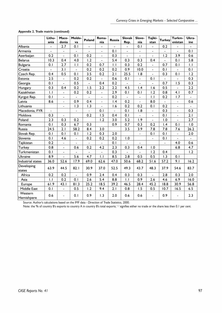
97
Currency Crises in Emerging Markets – Selected Comparative ...
CASE Reports No. 41
Appendix 2. Trade matrix (continued)
Lithu-ania
Mace-donia
Moldo-va
PolandRoma-
niaRussia
SlovakRep.
Slove-nia
Tajiki-stan
TurkeyTurkm-enistan
Ukra-ine
Albania - 2.7 0.1 - - - - 0.1 - 0.2 - -Armenia - - - - - 0.1 - - - - - 0.1Azerbaijan 0.2 - 0.1 0.2 - 0.3 - - - 1.2 3.9 0.6Belarus 10.3 0.4 4.0 1.2 - 5.4 0.3 0.3 0.4 - 0.1 5.8Bulgaria 0.1 2.7 1.1 0.2 0.7 1.1 0.3 0.2 - 0.7 0.1 1.1Croatia - 3.1 - 0.2 0.2 0.2 0.9 10.0 - 0.1 - 0.1Czech Rep. 0.4 0.5 0.1 3.5 0.2 2.1 25.5 1.8 - 0.3 0.1 1.2Estonia 2.5 - 0.2 0.2 - 0.6 0.1 - 0.1 - - 0.3Georgia 0.1 - 0.5 - 0.4 0.2 - - - 0.7 1.5 0.3Hungary 0.3 0.4 0.2 1.5 2.2 2.2 4.5 1.4 1.6 0.5 - 2.2Kazakhstan 1.1 - 0.2 0.2 - 2.9 0.1 0.1 1.2 0.8 4.1 0.7Kyrgyz Rep. 0.1 - - - - 0.2 - - 1.1 0.2 1.7 -Latvia 8.6 - 0.9 0.4 - 1.4 0.2 - 8.0 - - 0.6Lithuania - 1.3 1.3 - 1.6 0.2 0.2 0.1 0.2 - -Macedonia, FYR - - - 0.1 - 0.1 1.8 - 0.3 - 0.3Moldova 0.3 - 0.2 1.5 0.4 0.1 - - 0.1 - 2.1Poland 2.3 0.3 0.2 1.2 3.0 5.2 1.9 - 1.0 - 2.7Romania 0.1 0.3 6.7 0.3 0.9 0.7 0.3 0.2 1.4 0.1 1.0Russia 24.5 2.1 58.2 8.4 3.0 3.5 3.9 7.8 7.8 7.6 26.2Slovak Rep. 0.1 0.1 0.1 1.2 0.3 2.0 - 0.1 0.1 - 2.0Slovenia 0.1 4.6 - 0.2 0.2 0.2 1.0 - 0.1 - -Tajikistan 0.2 - - - - 0.1 - - - 4.0 0.6Turkey 0.8 - 0.6 0.2 4.2 2.3 0.3 0.4 1.0 6.8 4.7Turkmenistan 0.1 - - - - 0.3 - - 1.2 0.4 1.2Ukraine 8.9 - 5.6 4.7 1.1 8.5 2.8 0.5 0.5 1.3 0.1Industrial states 36.0 52.6 17.9 69.0 62.6 47.0 50.6 68.2 51.6 57.2 9.1 16.2Developingstates
63.9 44.5 82.1 30.9 37.0 52.5 49.3 43.7 48.3 37.9 54.6 83.7
Africa 0.2 0.2 - 0.9 2.4 0.4 0.3 0.3 - 2.8 0.3 2.0 Asia 1.1 0.2 0.1 2.6 5.4 8.8 1.1 0.9 2.6 4.6 6.9 16.0 Europe 61.9 43.1 81.3 25.2 18.5 39.2 46.5 28.4 45.2 18.8 30.9 56.8 Middle East 0.1 - 0.5 1.2 9.4 2.1 0.8 1.5 0.5 10.7 16.5 6.5 WesternHemishpere
0.6 - 0.1 0.9 1.3 2.0 0.6 0.6 - 0.9 - 2.3
Source: Author's calculations based on the IMF data - Direction of Trade Statistics, 2000.Note: the % of country B's exports to country A in country B's total exports; '-' signifies either no trade or the share less then 0.1 per cent.
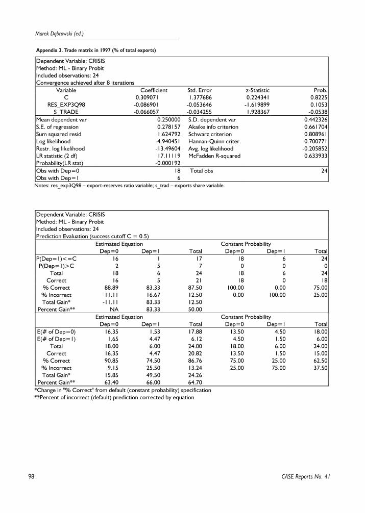
98
Marek D¹browski (ed.)
CASE Reports No. 41
Appendix 3. Trade matrix in 1997 (% of total exports)
Dependent Variable: CRISISMethod: ML - Binary ProbitIncluded observations: 24Convergence achieved after 8 iterations
Variable Coefficient Std. Error z-Statistic Prob.C 0.309071 1.377686 0.224341 0.8225
RES_EXP3Q98 -0.086901 -0.053646 -1.619899 0.1053S_TRADE -0.066057 -0.034255 1.928367 -0.0538
Mean dependent var 0.250000 S.D. dependent var 0.442326S.E. of regression 0.278157 Akaike info criterion 0.661704Sum squared resid 1.624792 Schwarz criterion 0.808961Log likelihood -4.940451 Hannan-Quinn criter. 0.700771Restr. log likelihood -13.49604 Avg. log likelihood -0.205852LR statistic (2 df) 17.11119 McFadden R-squared 0.633933Probability(LR stat) -0.000192Obs with Dep=0 18 Total obs 24Obs with Dep=1 6
Notes: res_exp3Q98 – export-reserves ratio variable; s_trad – exports share variable.
Dependent Variable: CRISISMethod: ML - Binary ProbitIncluded observations: 24Prediction Evaluation (success cutoff C = 0.5)
Estimated Equation Constant ProbabilityDep=0 Dep=1 Total Dep=0 Dep=1 Total
P(Dep=1)<=C 16 1 17 18 6 24P(Dep=1)>C 2 5 7 0 0 0
Total 18 6 24 18 6 24Correct 16 5 21 18 0 18
% Correct 88.89 83.33 87.50 100.00 0.00 75.00% Incorrect 11.11 16.67 12.50 0.00 100.00 25.00Total Gain* -11.11 83.33 12.50
Percent Gain** NA 83.33 50.00 Estimated Equation Constant Probability
Dep=0 Dep=1 Total Dep=0 Dep=1 TotalE(# of Dep=0) 16.35 1.53 17.88 13.50 4.50 18.00E(# of Dep=1) 1.65 4.47 6.12 4.50 1.50 6.00
Total 18.00 6.00 24.00 18.00 6.00 24.00Correct 16.35 4.47 20.82 13.50 1.50 15.00
% Correct 90.85 74.50 86.76 75.00 25.00 62.50% Incorrect 9.15 25.50 13.24 25.00 75.00 37.50Total Gain* 15.85 49.50 24.26
Percent Gain** 63.40 66.00 64.70*Change in "% Correct" from default (constant probability) specification**Percent of incorrect (default) prediction corrected by equation
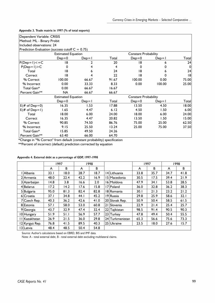
99
Currency Crises in Emerging Markets – Selected Comparative ...
CASE Reports No. 41
Appendix 3. Trade matrix in 1997 (% of total exports)
Dependent Variable: CRISISMethod: ML - Binary ProbitIncluded observations: 24Prediction Evaluation (success cutoff C = 0.75)
Estimated Equation Constant ProbabilityDep=0 Dep=1 Total Dep=0 Dep=1 Total
P(Dep=1)<=C 18 2 20 18 6 24P(Dep=1)>C 0 4 4 0 0 0
Total 18 6 24 18 6 24Correct 18 4 22 18 0 18
% Correct 100.00 66.67 91.67 100.00 0.00 75.00% Incorrect 0.00 33.33 8.33 0.00 100.00 25.00Total Gain* 0.00 66.67 16.67
Percent Gain** NA 66.67 66.67 Estimated Equation Constant Probability
Dep=0 Dep=1 Total Dep=0 Dep=1 TotalE(# of Dep=0) 16.35 1.53 17.88 13.50 4.50 18.00E(# of Dep=1) 1.65 4.47 6.12 4.50 1.50 6.00
Total 18.00 6.00 24.00 18.00 6.00 24.00Correct 16.35 4.47 20.82 13.50 1.50 15.00
% Correct 90.85 74.50 86.76 75.00 25.00 62.50% Incorrect 9.15 25.50 13.24 25.00 75.00 37.50Total Gain* 15.85 49.50 24.26
Percent Gain** 63.40 66.00 64.70*Change in "% Correct" from default (constant probability) specification**Percent of incorrect (default) prediction corrected by equation
Appendix 4. External debt as a percentage of GDP, 1997-1998
1997 1998 1997 1998A B A B A B A B
1 Albania 33.1 18.0 28.7 18.7 14 Lithuania 33.8 35.7 34.7 41.82 Armenia 48.0 22.4 42.2 16.9 15 Macedonia 30.5 17.5 39.4 21.93 Azerbaijan 14.8 3.8 16.6 2.0 16 Moldova 47.9 34.1 53.8 28.54 Belarus 17.2 14.2 17.6 15.8 17 Poland 36.0 32.8 36.2 38.35 Bulgaria 95.0 81.3 82.4 82.8 18 Romania 30.1 21.3 23.2 21.26 Croatia 37.1 34.8 44.1 45.2 19 Russia 29.8 25.9 58.6 32.17 Czech Rep. 40.3 36.2 42.6 41.0 20 Slovak Rep. 50.9 50.4 58.5 61.58 Estonia 57.1 58.0 53.0 60.8 21 Slovenia 22.9 21.4 25.4 25.79 Georgia 43.7 32.9 47.4 32.4 22 Tajikistan 98.5 91.4 90.5 90.3
10 Hungary 51.9 51.1 56.9 57.7 23 Turkey 47.8 49.4 50.4 55.511 Kazakhstan 26.9 21.5 36.0 29.8 24 Turkmenistan 65.3 56.6 75.6 73.312 Kyrgyz Rep. 76.8 41.5 89.5 40.3 25 Ukraine 23.5 18.0 27.6 15.713 Latvia 48.4 48.5 50.4 54.8
Source: Author's calculations based on EBRD, BIS and IMF data.Note: A - total external debt, B - total external debt excluding multilateral claims.
100
Marek D¹browski (ed.)
References
Abeysinghe T. (1999). "Thai Meltdown and Transmissionof Recession within ASEAN4 and NIE4". first draft.
Antczak R., Bogdankiewich S., Daneiko P., Po³omski K.,and Usowski V. (2000). "Impact of the Russian Crisis on theBelarussian Economy", CASE Studies and Analyses, No. 206,Warszaw.
Antczak R. (2001). "The Russian crisis of 1998". Forth-coming in CASE Report No. 40, Warsaw.
Baig T., Goldfajn I. (2000). "The Russian Default and theContagion to Brazi". IMF Working Paper,WP/00/160.
Burnside C., Eichenbaum M., Rebelo S. (2000). "On thefundamentals of self-fulfilling speculative attacks". NBERWorking Paper No. 7554, February.
Chang R., Majnoni G. (1999). "International Contagion:Implications for Policy". Paper prepared for the World BankConference on "Contagion: How It Spreads and How it CanBe Stopped?" ,Washington, February 3-4, 2000.
D¹browski M. (1999). " ". CASE WorkingPapers No. 198, Warsaw.
Dornbusch R., Park Y.C., Claessens S. (2000). "Conta-gion: How it spreads and How it can be stopped?".
Drazen A. (1999). "Political Contagion in CurrencyCrises". NBER Working Paper No. 7211, July.
EBRD (2000). "Transition report update". May 2000,London.
Edwards S. (1998). "Interest rate volatility, capital controlsand contagion". NBER Working Paper No. 6756, October.
Eichengreen B., Rose A.K., Wyplosz C. (1996). "Conta-gious Currency Crises". NBER Working Paper No. 5681,July.
Favero C., Giavazzi F. (1999). "Looking for contagion:Evidence from the 1992 ERM crisis". Paper prepared for theUNU/WIDER project on "Financial contagion: How itspreads and how it can be stopped?".
Flood R.P., Marion N.P. (1998). "Perspectives on theRecent Currency Crisis Literature". IMF Working Paper,WP/98/130, September.
Forbes K. (2000a). "Identification through heteroskedas-ticity: Measuring 'contagion' between Argentinean and Mex-ican sovereign bonds". NBER Working Paper No. 7493, Jan-uary.
Forbes K. (2000b). "How Important is Trade in the Inter-national Spread of Crises". Paper prepared for the NBERconference on Currency Crises Prevention, December 9.
Forbes K., Rigobon R. (1999a). "No Contagion, OnlyInterdependence: Measuring Stock Market Co-move-ments". NBER Working Paper No. 7267, July.
Forbes K., Rigobon R. (1999b). "Measuring Contagion:Conceptual and Empirical Issues'. Paper prepared for the
November 19-20, 1999 UNU-WIDER conference on Finan-cial Contagion held in Helsinki, Finland.
Fries S., Raiser M., Stern N. (1999). "Stress test forreforms". Economics of Transitions, Vol. 7 (2), 535–567.
Froot K.A., O'Connell P.G.J., Seasholes M.S. (1999). "ThePortfolio Flows of International Investors".
Gelos R.G., Sahay R. (1999). "Financial Market Spilloversin Transition Economies". IMF Working Paper,WP/99/, pre-liminary.
Glick R., Rose A.K. (1999). "Contagion and trade. Whyare currency crises regional?". Journal of InternationalMoney and Finance, Vol. 18 (1999), 603-617.
Goldberg L., Dages G., Kinney D. (1999). "Lending inEmerging Markets: Foreign and Domestic Banks Com-pared". (working version).
Gregorio J., Valdes R.O. (1999). "Crisis Transmission:Evidence from the Debt, Tequila, and Asian Flu Crise".,Paper prepared for the UNU/WIDER project on "Financialcontagion: How it spreads and how it can be stopped?".
Hajivassiliou V. (1994). "A simulation estimation analysisof the external debt crises of developing countries". Journalof Applied Econometrics, Vol. 9, p. 109–131.
Hajivassiliou V., McFadden D. (1990). "The Method ofSimulated Scores, with Application to Models of ExternalDebt Crises". Cowles Foundation Discussion Paper No.967.
Hajivassiliou V., Ruud P.A. (1994). "Classical EstimationMethods for LDV Models Using Simulation". Handbook ofEconometrics, Vol. IV, pp. 2384–2441.
IMF (1998). "Exchange Arrangements and ExchangeRestrictions". IMF Annual Report, Washington.
IMF (1999a). "Exchange Arrangements and ExchangeRestrictions". IMF Annual Report, Washington.
IMF (1999b). "International Financial Contagion". ch. IIIin World Economic Outlook, p. 66–86, Washington.
IMF (1999c). "Kyrgyz Republic: Recent Economic Devel-opments". IMF Staff Country Report No. 99/31, April.
IMF (1999d). "Ukraine: Recent Economic Develop-ments". IMF Staff Country Report No. 99/42, May.
IMF (1999e). "Republic of Lithuania: Selected Issues andStatistical Appendix". IMF Staff Country Report No. 99/96,September.
IMF (1999f). "Republic of Moldova: Recent EconomicDevelopments". IMF Staff Country Report No. 99/110, Sep-tember.
IMF (2000a). "Direction of Trade Statistics Yearbook".Washington DC.
IMF (2000b). "Republic of Kazakhstan: Selected Issuesand Statistical Appendix". IMF Staff Country Report No.00/29, March.
IMF (2000c). "Georgia: Recent Economic Developmentsand Selected Issues". IMF Staff Country Report No. 00/68,May.
CASE Reports No. 41
101
Currency Crises in Emerging Markets – Selected Comparative ...
Jeanne O. (1997). "Are currency crises self-fulfilling? ATest". Journal of International Economics Vol. 43, p.263–286.
Jeanne O. (1999). "Currency Crises: A Perspective onRecent Theoretical Developments". Discussion Paper No.2170 CEPR, June.
Jeanne O., Masson P. (1999). "'Currency crises, sunspotsand Markov-switching regimes". Journal of InternationalEconometrics, Vol. 50, p. 327–350.
Kaminsky G., Reinhart C.M. (1999). "The Twin Crises: TheCause of Banking and Balance-of-Payments Problems". Amer-ican Economic Review, Vol. 89, No. 3, June, p. 473– 500.
Kaminsky G., Schmukler S. (1999). "What triggers mar-ket jitters? A chronicle of the Asian crisis". Journal of Inter-national Money and Finance, Vol. 18 (1999), p. 537–560.
Kaminsky G., Lyons R., Schmukler S. (1999). "Managers,Investors, and Crises: Mutual Fund Strategies in EmergingMarkets", draft.
Lane P.R., Milesi-Ferretti G.M. (2000). "External CapitalStructure: Theory and Evidence". IMF WorkingPaper,WP/00/152, August.
Linne T. (1999). "Contagion Effects of Central and EastEuropean Currency Crises"., Discussion Papers, No. 96,Institute for Economic Research Halle, April.
Markiewicz M. (2001). "The Ukrainian crisis of 1998".forthcoming in CASE Report No. 40, Warsaw.
Masson P. (1998). "Contagion: Monsoonal Effects,Spillovers, and Jumps Between Multiple Equilibria". IMFWorking Paper,WP/98/142, September.
Masson P. (1999). "Contagion: macroeconomic modelswith multiple equilibria". Journal of International Money andFinance, Vol. 18 (1999), p. 587–602.
Pritsker M. (2000). "The Channels for Financial Conta-gion". UNU/WIDER Contagion Project.
Radziwi³³ A. (2001). "The Moldovian crisis of 1998".forthcoming in CASE Report No. 40, Warsaw.
Rigobon R. (1999). "On measurement of the Interna-tional Propagation of Shocks". NBER Working Paper No.7354, September.
Rigobon R. (2000). "Identification Through Het-eroskedasticity: Measuring "Contagion" Between Argen-tinean and Mexican Sovereign Bond". NBER Working PaperNo. 7493, January.
Rijckeghem C., Weder B. (1999a). "Financial Contagion:Spillovers through Banking Centers". Paper prepared as partof a project on contagion supported by WIDER and theWorld Bank.
Rijckeghem C., Weder B. (1999b). "Source of Conta-gion: Finance or Trade?". IMF Working Paper, WP/99/146,October.
Sasin M. (2000). "Predicting Currency Crises. The Ulti-mate Significance of Macroeconomic fundamentals in LinearSpecifications (with Nonlinear extension)". MS dissertation,Katholieke Universiteit Leuven
Schinasi G.J., Smith, R.T. (1999). "Portfolio Diversifica-tion, Leverage, and Financial Contagion". IMF WorkingPaper, WP/99/136.
CASE Reports No. 41

103
Currency Crises in Emerging Markets – Selected Comparative ...
CASE Reports No. 41
6.1. Introduction
The 1990s have witnessed five waves of financial turbu-lence in international capital markets: the EMS crisis of1992–1993, the Mexican peso crisis and its aftermath(1994–1995), the Asian crisis of 1997, the Russian crisis andconsequent crashes in several former Soviet Union coun-tries (FSU), and finally Brazil and Turkey. Financial crises arenot the new phenomena, and have occurred with occasion-ally higher or lower intensities for at least the last two cen-turies (a good historical panorama is provided, e.g., byBordo and Schwartz, 1999 and Kindleberger, 2000). How-ever, along with proceeding globalization, the nature offinancial collapses has been changing.
The literature dealing with the causes of financial crisesis vast and, especially in recent years, much progress hasbeen recorded in this field. However, the consequences offinancial turbulence are rarely examined. The establishmentof the set of 'early warning indicators' is of course highlydesirable since it helps to predict crises, but the diagnosis ofthe performance of economies after crises is at least equal-ly important. For example, were it the case that crises are acrude but optimal way of removing the imbalances in aneconomy, it would then become unnecessary to analyzeindexes of financial market pressure (what brings question-able results anyway) or other ways of measuring potentialvulnerabilities. Moreover, transition economies are oftenexcluded from analyses. The most serious reason for this isperhaps the lack of good quality data. Also, the transitionprocess itself embraces great systemic changes to the func-tioning of economies, so it is extremely difficult to separatethe effects of these changes from those stemming fromcrises.
In the public discussion about financial turbulence (thathas been very vivid recently and took part on a popular levelalso, e.g. in international press) the majority of voices seemto share the view that crises are unfavorable incidents thatshould be avoided using all possible means. The argumentsusually point at the severe costs the crashes bring [Stiglitz,1998]. On the other hand, in some cases authors emphasize
the positive impact of turmoil on the economic policies, andthe progress of reforms [e.g. Bulgarian crisis of 1996; cf.IMF, 1999] or developments in the real sector and function-ing of an economy in general [e.g. Russian crisis of 1998; cf.Westin, 1999].
Actually, it turns out that that much evidence on whichthe reasoning in both directions hinges is rather weak. Cer-tainly, countries that underwent problems with financial sta-bility are very different, and so were natures of the crisesand their consequences. Thus, it is impossible to find gen-erally binding rules assigned to crises' consequences. Yet, itis possible to discover statistical regularities in the results ofcrises and to present some stylized types of interactionsthat tend to strengthen either negative or positive out-comes.
This paper attempts to investigate the consequences offinancial crises from an international perspective. It does soby analyzing the behavior of several macroeconomic vari-ables before and after episodes of financial turbulence anddescribes both their positive and negative consequences.The analysis is limited to the 1990s and covers mostly tran-sition economies. The time constrains were set in order tofocus on recent developments in world financial markets;the inclusion of considerable number of transitioneconomies was motivated by the willingness to fill in a gapexisting in the literature.
The paper also analyzes the channels through whichcrises affect various economic and social spheres. In addi-tion, some checks are carried to see whether and underwhat circumstances crises can have a lasting and positive (orat least neutral) influence on economies in the medium termperspective. The paper further focuses on the question howlong the post-crisis effects are present and if the recoveryprocess removes the pre-crisis imbalances.
The rest of the paper is organized as follows. In sectiontwo a brief survey of literature dealing with consequencesof financial crises is presented. Section three is devoted tothe presentation of graphical analysis of the behavior ofselected macroeconomic variables in a period before andafter a crisis. Various notions of costs related to financial tur-moil are dealt with in section four. Section five discusseswhat the possible positive outcomes of crises are and under
Part VI.The Economic and Social Consequences of Financial CrisesMonika B³aszkiewicz, Wojciech Paczyñski
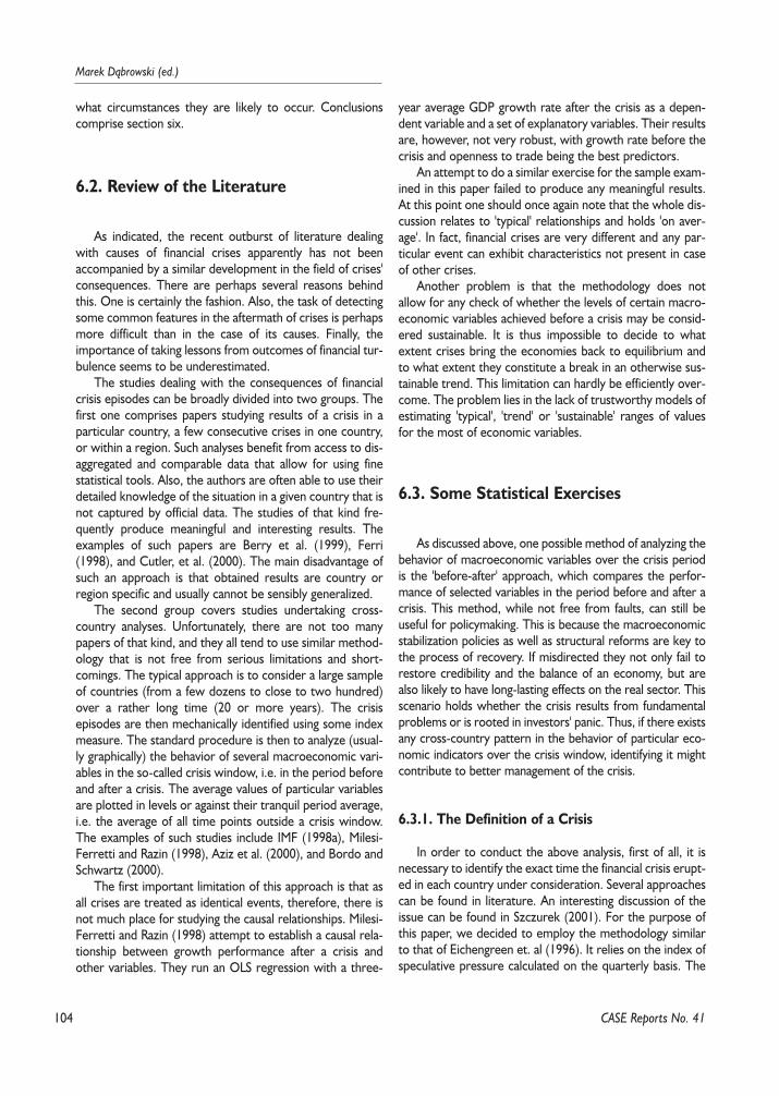
104
Marek D¹browski (ed.)
CASE Reports No. 41
what circumstances they are likely to occur. Conclusionscomprise section six.
6.2. Review of the Literature
As indicated, the recent outburst of literature dealingwith causes of financial crises apparently has not beenaccompanied by a similar development in the field of crises'consequences. There are perhaps several reasons behindthis. One is certainly the fashion. Also, the task of detectingsome common features in the aftermath of crises is perhapsmore difficult than in the case of its causes. Finally, theimportance of taking lessons from outcomes of financial tur-bulence seems to be underestimated.
The studies dealing with the consequences of financialcrisis episodes can be broadly divided into two groups. Thefirst one comprises papers studying results of a crisis in aparticular country, a few consecutive crises in one country,or within a region. Such analyses benefit from access to dis-aggregated and comparable data that allow for using finestatistical tools. Also, the authors are often able to use theirdetailed knowledge of the situation in a given country that isnot captured by official data. The studies of that kind fre-quently produce meaningful and interesting results. Theexamples of such papers are Berry et al. (1999), Ferri(1998), and Cutler, et al. (2000). The main disadvantage ofsuch an approach is that obtained results are country orregion specific and usually cannot be sensibly generalized.
The second group covers studies undertaking cross-country analyses. Unfortunately, there are not too manypapers of that kind, and they all tend to use similar method-ology that is not free from serious limitations and short-comings. The typical approach is to consider a large sampleof countries (from a few dozens to close to two hundred)over a rather long time (20 or more years). The crisisepisodes are then mechanically identified using some indexmeasure. The standard procedure is then to analyze (usual-ly graphically) the behavior of several macroeconomic vari-ables in the so-called crisis window, i.e. in the period beforeand after a crisis. The average values of particular variablesare plotted in levels or against their tranquil period average,i.e. the average of all time points outside a crisis window.The examples of such studies include IMF (1998a), Milesi-Ferretti and Razin (1998), Aziz et al. (2000), and Bordo andSchwartz (2000).
The first important limitation of this approach is that asall crises are treated as identical events, therefore, there isnot much place for studying the causal relationships. Milesi-Ferretti and Razin (1998) attempt to establish a causal rela-tionship between growth performance after a crisis andother variables. They run an OLS regression with a three-
year average GDP growth rate after the crisis as a depen-dent variable and a set of explanatory variables. Their resultsare, however, not very robust, with growth rate before thecrisis and openness to trade being the best predictors.
An attempt to do a similar exercise for the sample exam-ined in this paper failed to produce any meaningful results.At this point one should once again note that the whole dis-cussion relates to 'typical' relationships and holds 'on aver-age'. In fact, financial crises are very different and any par-ticular event can exhibit characteristics not present in caseof other crises.
Another problem is that the methodology does notallow for any check of whether the levels of certain macro-economic variables achieved before a crisis may be consid-ered sustainable. It is thus impossible to decide to whatextent crises bring the economies back to equilibrium andto what extent they constitute a break in an otherwise sus-tainable trend. This limitation can hardly be efficiently over-come. The problem lies in the lack of trustworthy models ofestimating 'typical', 'trend' or 'sustainable' ranges of valuesfor the most of economic variables.
6.3. Some Statistical Exercises
As discussed above, one possible method of analyzing thebehavior of macroeconomic variables over the crisis periodis the 'before-after' approach, which compares the perfor-mance of selected variables in the period before and after acrisis. This method, while not free from faults, can still beuseful for policymaking. This is because the macroeconomicstabilization policies as well as structural reforms are key tothe process of recovery. If misdirected they not only fail torestore credibility and the balance of an economy, but arealso likely to have long-lasting effects on the real sector. Thisscenario holds whether the crisis results from fundamentalproblems or is rooted in investors' panic. Thus, if there existsany cross-country pattern in the behavior of particular eco-nomic indicators over the crisis window, identifying it mightcontribute to better management of the crisis.
6.3.1. The Definition of a Crisis
In order to conduct the above analysis, first of all, it isnecessary to identify the exact time the financial crisis erupt-ed in each country under consideration. Several approachescan be found in literature. An interesting discussion of theissue can be found in Szczurek (2001). For the purpose ofthis paper, we decided to employ the methodology similarto that of Eichengreen et. al (1996). It relies on the index ofspeculative pressure calculated on the quarterly basis. The

105
Currency Crises in Emerging Markets – Selected Comparative ...
CASE Reports No. 41
index is a combination of the exchange rate, interest rateand domestic reserves of foreign exchange. The pressureincreases as the exchange rate depreciates, reserves depleteand interest rates go up. If the attack is successful devalua-tion occurs, but authorities may try to defend the currencyby running down international reserves or raising interestrates. The crisis episode is defined as an unusually rapidincrease in the index. A formal presentation can be found inAppendix 1.
The presented methodology captured 27 crisis episodeswith Brazil, Kazakhstan, Kyrgyz Republic, Moldova andUkraine suffering from financial turbulence twice over thestudied period.
6.3.2. The Sample
The sample spans from 1990 to 1999 and covers 43countries. The list of all countries included can be found inAppendix 2. Such a choice was determined by the aim toconcentrate on the recent crise only (i.e. the financial criseof the 1990s) and to include as many transition countries (inparticular the FSU countries) as possible. In this respect thestatistical analysis presented below differs from the one con-ducted in several other studies.
6.3.3. Data
Having identified crisis episodes, it is necessary to evalu-ate the performance of economic variables that according totheory can be affected by a financial crisis. The rationalitybehind the choice of indicators presented below lies in twofacts. First, the deviation of these variables from their equi-librium levels (that can somehow be established) has ledmany countries to problems and was recognized byresearches as central to the incidences of crise [e.g. seeKaminsky et al., 1998; Flood et al., 1998]. Then, if the crisiswas to help to restore the balance in an economy, oneshould observe striking changes in the performance of for-mer predictors of crises. Second, as social repercussions ofa crisis also lie within our interests, the analysis cannot beconstraint to macroeconomic indicators only. For instance,households can be worse off due to the decline in the valueof their assets or because of a post-crisis economic contrac-tion affecting them through various channels (see section 4for a more detailed discussion).
The analysis below focuses on the following indicators:– GDP per capita, – GDP growth,– inflation,– real and nominal interest rates,– current account balance,– capital flows, exchange rate,
– changes in government and private consumption,– investment rates,– trade performance– unemployment rate. The main source of data is the International Financial
Statistics (IFS) of the International Monetary Found (IMF).GDP data are taken from the IMF's World Economic Out-look database (May 2001). Additional data sources (such asAsian Development Bank, and the countries' statistical agen-cies) were also used in some instances. Unemploymentrates and nominal wages come from the International LaborOrganization (ILO) and the World Health Organization(WHO), respectively. GDP per capita in PPP terms is fromWHO.
6.3.4. Economic Performance before and afterthe Crisis
The following discussion focuses on the behavior ofselected macroeconomic variables in the 'crisis window'. Westart from checking some characteristics of countries in oursample. Assessing the level of development of analyzedcountries is important as it certainly influences eventualimpact of financial crises. In poor countries crisis spilloversare likely to be more difficult to manage. In particular, theimpact on the social sphere might have significant conse-quences, e.g. rising poverty.
In order to see the development level of the countriesin the sample we calculated average GDP per capita. As evi-dent from the picture, on average (median), countries under
Figure 6-1. GDP per capita in a crisis window, USD
0
1000
2000
3000
4000
5000
c-3 c-2 c-1 crisis c+1 c+2 c+3
nominal (median) in PPP terms (median)
Note: Graph plots a median GDP per capita on annual basis in a cri-sis window of three years before and after a crisis.
Sources: IMF IFS (2001), WHO (2001).
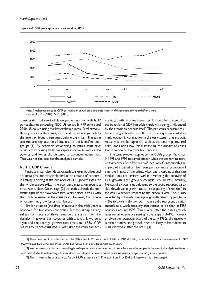
106
Marek D¹browski (ed.)
CASE Reports No. 41
consideration fall short of developed economies with GDPper capita not exceeding 4500 US dollars in PPP terms and2500 US dollars using market exchange rates. Furthermore,three years after the crises, income still does not go back tothe levels achieved three years before the crises. The samepatterns are repeated in all but one of the identified sub-groups [1]. By definition, developing countries must haveminimally increasing GDP per capita in order to reduce thepoverty and lower the distance to advanced economies.This was not the case for the analyzed sample.
6.3.4.1. GDP GrowthFinancial crises often deteriorate into systemic crises and
are most pronouncedly reflected in the erosion of econom-ic activity. Looking at the behavior of GDP growth rates forthe whole sample (ALL), the economic stagnation around acrisis year is clear. On average [2], countries already demon-strate signs of the slowdown two years before a crisis withthe 1.5% recession in the crisis year. However, from thereon economies grow faster than before.
Similar situation (the drop of output in the crisis year) isobserved for transition economies. But this group alreadysuffers from recession three years before a crisis. Then thesituation improves but, together with a crisis, it worsensagain and the average growth rate drops to -6.5%. GDPreturns to its pre-crisis level a year after the crisis and eco-
nomic growth resumes thereafter. It should be stressed thatthe behavior of GDP in a crisis window is strongly influencedby the transition process itself. The pre-crisis recession visi-ble in the graph often results from the experience of dra-matic economic contraction in the early stages of transition.Actually, a simple approach, such as the one implementedhere, does not allow for dismantling the impact of crisesfrom the one of the transition process.
The same problem applies to the FSU98 group. The crisesin 1998 and 1999 occurred exactly when the economies start-ed to recover after a few years of recession. Consequently, theimpact of a transition itself was perhaps more pronouncedthan the impact of the crises. Also, one should note that themedian does not perform well in describing the behavior ofGDP growth in this group of countries around 1998. Actually,five out of six countries belonging to the group recorded a siz-able slowdown in growth rates (or deepening of recession) inthe crisis year with respect to the previous year. This is alsoreflected by arithmetic average of growth rates dropping from4.2% to 0.4% in this period. The crisis did represent a majorsetback to a weak recovery that started to be seen in FSUcountries around 1997. Three years after the crises growthrates remained positive staying in the range of 3–4%. Howev-er, given the recession record of the early 1990s, the recoveryis rather modest and growth rates are likely to be reduced in2001 (third year after the crisis) [3].
[1] These are crises in transition economies (TR), crises in FSU countries in 1998 and 1999 (FSU98), crises in South-East Asian economies in 1997(ASIA97), and Latin American crises (LAM). See Annex 2 for a detailed sample description.
[2] In order to reduce distortions resulting from large variation in some economic variables across the sample, in the statistical analysis median wasused instead of arithmetic average. Unless otherwise indicated, whenever in the paper we write 'average' it actually means 'median'.
[3] The last year in the crisis window for the FSU98 group is the IMF forecast from May 2001 and therefore might be changed.
Figure 6-2. GDP per capita in a crisis window, USD
0
1000
2000
3000
4000
5000
c-3 c-2 c-1 crisis c+1 c+2 c+3
ALL TR FSU98
ASIA97 LAM
Note: Graph plots a median GDP per capita on annual basis in a crisis window of three years before and after a crisis.Sources: IMF IFS (2001), WHO (2001).

107
Currency Crises in Emerging Markets – Selected Comparative ...
In South-East Asia, the 1997 crisis brought the averagerate of output growth down from more than 8% in 1994 toan estimated 4.8% in 2001. In terms of the scale of growthcontraction, the ASIA97 group stands out in the entireexamined sample (with the recession of 7.4% a year afterthe shock). However, this group is also exceptional in termsof its pre-crisis stance, when the Asian economies recordedastounding growth rates of around 8% annually. Further-more, the 1997 crisis was not a typical one with chronic
internal or external imbalances playing a decisive role. Theproblem was more complex. In short, apart from the Philip-pines, the crises were driven by the developments in thecapital account. 'Asian Tigers' were growing fast, attractinghuge amounts of foreign capital (on average 40% of GDP in1990–1996) that led to an investment boom. After the cri-sis, investors discounted the market that deepened therecession and reduced the growth stimulus stemming fromincreased competitiveness.
CASE Reports No. 41
Figure 6-3. Real GDP growth (median), %
-10
-8
-6
-4
-2
0
2
4
6
8
10
c-3 c-2 c-1 crisis
year
c+1 c+2 c+3
ALL TR FSU98ASIA97 LAM
Source: IMF, WEO database.
Figure 6-4. Real GDP growth differential (median), %
-12
-10
-8
-6
-4
-2
0
2
4
6
8
c-3 c-2 c-1 crisis
year
c+1 c+2 c+3
ALL TR FSU98ASIA97 LAM
Note: GDP growth differential is defined as a difference between a crisis country growth rate and advanced economies average GDP growth (theaggregate is provided by the IMF, World Economic Outlook 2001 database).
Source: IMF, WEO database.
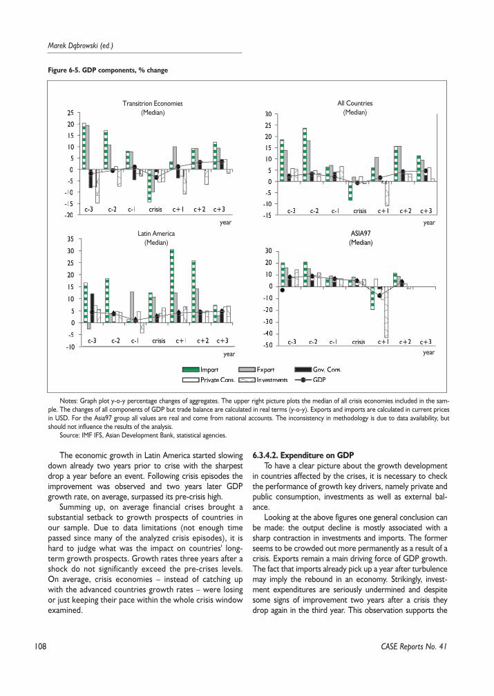
108
Marek D¹browski (ed.)
The economic growth in Latin America started slowingdown already two years prior to crise with the sharpestdrop a year before an event. Following crisis episodes theimprovement was observed and two years later GDPgrowth rate, on average, surpassed its pre-crisis high.
Summing up, on average financial crises brought asubstantial setback to growth prospects of countries inour sample. Due to data limitations (not enough timepassed since many of the analyzed crisis episodes), it ishard to judge what was the impact on countries' long-term growth prospects. Growth rates three years after ashock do not significantly exceed the pre-crises levels.On average, crisis economies – instead of catching upwith the advanced countries growth rates – were losingor just keeping their pace within the whole crisis windowexamined.
6.3.4.2. Expenditure on GDPTo have a clear picture about the growth development
in countries affected by the crises, it is necessary to checkthe performance of growth key drivers, namely private andpublic consumption, investments as well as external bal-ance.
Looking at the above figures one general conclusion canbe made: the output decline is mostly associated with asharp contraction in investments and imports. The formerseems to be crowded out more permanently as a result of acrisis. Exports remain a main driving force of GDP growth.The fact that imports already pick up a year after turbulencemay imply the rebound in an economy. Strikingly, invest-ment expenditures are seriously undermined and despitesome signs of improvement two years after a crisis theydrop again in the third year. This observation supports the
CASE Reports No. 41
Figure 6-5. GDP components, % change
-20
-15
-10
-5
0
5
10
15
20
25
-15
-10
-5
0
5
10
15
20
25
30
-10
-5
0
5
10
15
20
25
30
35
c-3 c-2 c-1 crisis c+1 c+2 c+3
ASIA97(Median)
-50
-40
-30
-20
-10
0
10
20
30
Import Exportorto Gov. Cons.Private Consonso . Investmentente stst GDP
Latin America(Median)
Transitrion Economies(Median)
year
All Countries(Median)
c-3 c-2 c-1 crisis c+1 c+2 c+3
c-3 c-2 c-1 crisis c+1 c+2 c+3
c-3 c-2 c-1 crisis c+1 c+2 c+3
year year
year
Notes: Graph plot y-o-y percentage changes of aggregates. The upper right picture plots the median of all crisis economies included in the sam-ple. The changes of all components of GDP but trade balance are calculated in real terms (y-o-y). Exports and imports are calculated in current pricesin USD. For the Asia97 group all values are real and come from national accounts. The inconsistency in methodology is due to data availability, butshould not influence the results of the analysis.
Source: IMF IFS, Asian Development Bank, statistical agencies.
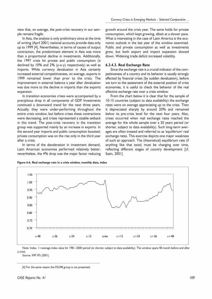
109
Currency Crises in Emerging Markets – Selected Comparative ...
view that, on average, the post-crisis recovery in our sam-ple remains fragile.
In Asia, the analysis is only preliminary since at the timeof writing (April 2001) national accounts provide data onlyup to 1999 [4]. Nevertheless, in terms of causes of outputcontraction, the predominant element in Asia was morethan a proportional decline in investments. Additionally,the 1997 crisis hit private and public consumption (itdeclined by 10% and 2% (y-o-y) respectively) as well asimports. While currency devaluation in Asia certainlyincreased external competitiveness, on average, exports in1999 remained lower than prior to the crisis. Theimprovement in external balance a year after devaluationwas due more to the decline in imports than the exportsexpansion.
In transition economies crises were accompanied by aprecipitous drop in all components of GDP. Investmentscontinued a downward trend for the next three years.Actually, they were under-performing throughout theentire crisis window, but before crises these contractionswere decreasing, and crises represented a sizable setbackin this trend. The post-crisis recovery in the transitiongroup was supported mainly by an increase in exports. Inthe second year imports and public consumption boosted;private consumption was on the rise only in the third yearafter a crisis.
In terms of the deceleration in investment demand,Latin American economies performed relatively better;nevertheless, the 4% drop was the major factor reducing
growth around the crisis year. The same holds for privateconsumption, which kept growing, albeit at a slower pace.What is interesting in the case of Latin America is the eco-nomic outlook in the last year of the window examined.Public and private consumption as well as investmentsgrew, but both export and import expansion sloweddown. Widening trade deficit increased volatility.
6.3.4.3. Real Exchange RateSince the exchange rate is a crucial indicator of the com-
petitiveness of a country and its behavior is usually stronglyaffected by financial crises (by sudden devaluation), beforewe turn to the assessment of the external position of crisiseconomies, it is useful to check the behavior of the realeffective exchange rate over a crisis window.
From the chart below it is clear that for the sample of10-15 countries (subject to data availability) the exchangerates were on average appreciating up to the crisis. Thenit depreciated sharply by around 20% and remainedbelow its pre-crisis level for the next four years. Also,crises occurred when real exchange rates reached theaverage for the whole sample over a 20 years period (orshorter, subject to data availability). Such long-term aver-ages are often treated and referred to as 'equilibrium' realexchange rates. This exercise depicts one major weaknessof such an approach. The (theoretical) equilibrium rate (ifanything like that exist) must be changing over time,reflecting different stages of country development [cf.Sasin, 2001].
CASE Reports No. 41
[4] For the same reason the FSU98 group is not presented.
Figure 6-6. Real exchange rate in a crisis window, monthly data, index
0.70
0.75
0.80
0.85
0.90
0.95
1.00
1.05
c-48 c-36 c-24 c-12 crisis c+12 c+24 c+36 c+48
Note: Index, 1=average index value for 1981–2000 period (or shorter, subject to data availability). The window spans 48 month before and aftera crisis.
Source: IMF IFS (2001).
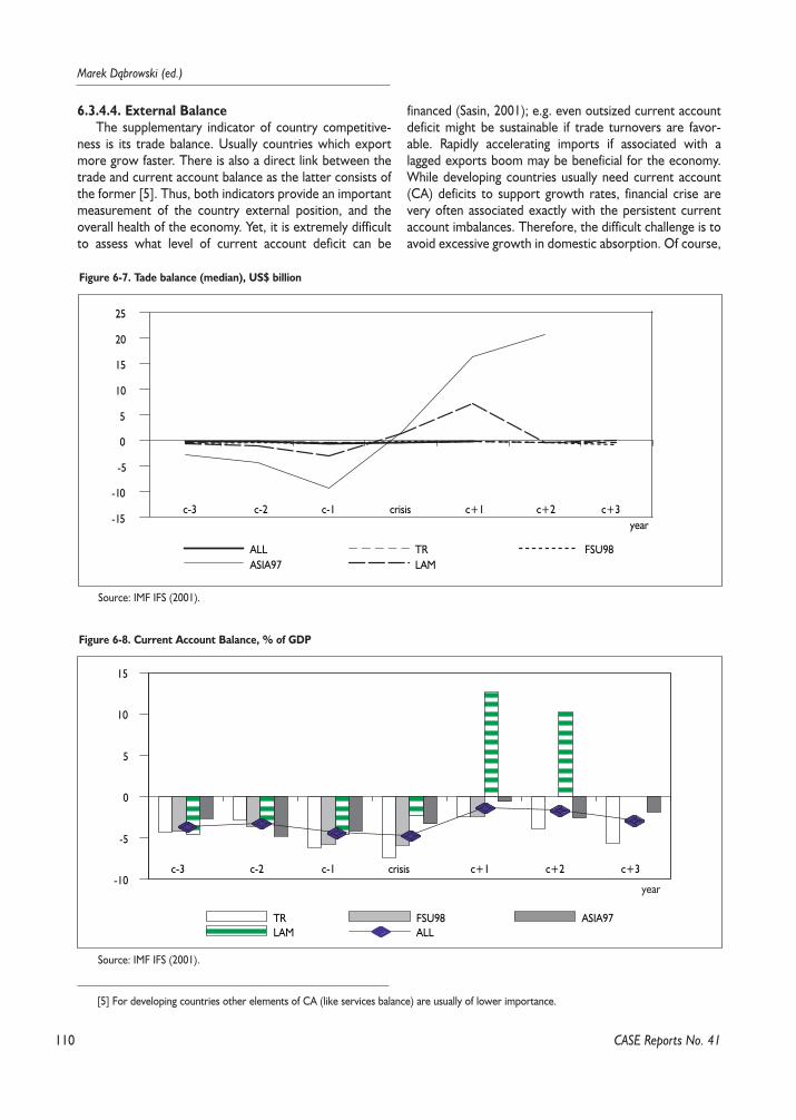
110
Marek D¹browski (ed.)
6.3.4.4. External BalanceThe supplementary indicator of country competitive-
ness is its trade balance. Usually countries which exportmore grow faster. There is also a direct link between thetrade and current account balance as the latter consists ofthe former [5]. Thus, both indicators provide an importantmeasurement of the country external position, and theoverall health of the economy. Yet, it is extremely difficultto assess what level of current account deficit can be
financed (Sasin, 2001); e.g. even outsized current accountdeficit might be sustainable if trade turnovers are favor-able. Rapidly accelerating imports if associated with alagged exports boom may be beneficial for the economy.While developing countries usually need current account(CA) deficits to support growth rates, financial crise arevery often associated exactly with the persistent currentaccount imbalances. Therefore, the difficult challenge is toavoid excessive growth in domestic absorption. Of course,
CASE Reports No. 41
[5] For developing countries other elements of CA (like services balance) are usually of lower importance.
Figure 6-7. Tade balance (median), US$ billion
-15
-10
-5
0
5
10
15
20
25
c-3 c-2 c-1 crisisyear
c+1 c+2 c+3
ALL TR FSU98ASIA97 LAM
Source: IMF IFS (2001).
Figure 6-8. Current Account Balance, % of GDP
-10
-5
0
5
10
15
TR FSU98 ASIA97LAM ALL
c-3 c-2 c-1 crisis c+1 c+2 c+3
year
Source: IMF IFS (2001).

111
Currency Crises in Emerging Markets – Selected Comparative ...
every country is specific, and so are roots underlying theexcess of investments over savings, but the outcome is thesame – a fragile external position.
From the above picture it is clear that all countries inthe sample suffered from persistent current accountimbalances. Moreover, on average, our "crise sample" sup-ports the common view, that a CA deficit oscillatingaround 5% of GDP is a precarious one and should be a"warning flag" for policy makers. As for sub-groups, the
biggest savings-investments gap is evident in transitioneconomies. A year before a crisis the average deficit forthese countries was equal to 7.4% of GDP.
Interestingly, the advantageous role of the weak curren-cy (as a result of devaluation) associated with financial crash-es was not strongly supported by the data. The impact ontrade balance proved to be limited. On average, trade bal-ance was worsening until one year before crises not only forthe whole sample, but also for individual sub-samples. Then,
CASE Reports No. 41
Figure 6-10. Exports growth (median), % change
-20
-10
0
10
20
30
c-3 c-2 c-1 crisis c+1 c+2 c+3
TR FSU98 ASIA97LAM ALL
Source: IMF IFS (2001).
Figure 6-9. Imports growth (median), % change
-40
-30
-20
-10
0
10
20
30
40
c-3 c-2 c-1 crisis c+1 c+2 c+3
TR FSU98 ASIA97LAM ALL
year
Source: IMF IFS (2001).
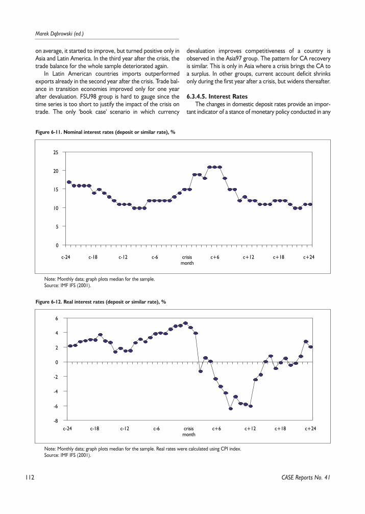
112
Marek D¹browski (ed.)
on average, it started to improve, but turned positive only inAsia and Latin America. In the third year after the crisis, thetrade balance for the whole sample deteriorated again.
In Latin American countries imports outperformedexports already in the second year after the crisis. Trade bal-ance in transition economies improved only for one yearafter devaluation. FSU98 group is hard to gauge since thetime series is too short to justify the impact of the crisis ontrade. The only 'book case' scenario in which currency
devaluation improves competitiveness of a country isobserved in the Asia97 group. The pattern for CA recoveryis similar. This is only in Asia where a crisis brings the CA toa surplus. In other groups, current account deficit shrinksonly during the first year after a crisis, but widens thereafter.
6.3.4.5. Interest RatesThe changes in domestic deposit rates provide an impor-
tant indicator of a stance of monetary policy conducted in any
CASE Reports No. 41
Figure 6-12. Real interest rates (deposit or similar rate), %
-8
-6
-4
-2
0
2
4
6
c-24 c-18 c-12 c-6 crisismonth
c+6 c+12 c+18 c+24
Note: Monthly data; graph plots median for the sample. Real rates were calculated using CPI index.Source: IMF IFS (2001).
Figure 6-11. Nominal interest rates (deposit or similar rate), %
0
5
10
15
20
25
c-24 c-18 c-12 c-6 crisismonth
c+6 c+12 c+18 c+24
Note: Monthly data; graph plots median for the sample. Source: IMF IFS (2001).

113
Currency Crises in Emerging Markets – Selected Comparative ...
particular country. Reflecting changes in various spheres ofthe economy, interest rates affect other policies (e.g. theroom for maneuver of fiscal policy is subject to cost of debtservicing) as well as consumers and producers behavior(including expectations) through various transition channels[Mishkin, 1996; Bernanke and Geritler, 1995]. High interestrates are usually a feature of so-called emerging markets thathave to pay high-risk premium to attract capital.
The purpose of this paper is not to discuss the theorybehind the interest rate policy. From the perspective of ouranalysis the behavior of interest rates is interesting for onemajor reason. In the onset of financial crises, in order todefend the exchange rate and stop fleeing capital, interestrates usually go up. After a crisis rising inflation drives nomi-nal interest rates up. This brings recessionary tendencies andexacerbates uncertainty related to the fact that high interestrates increase the probability that productive investments arenot undertaken [see Mishkin, 1996]. If this was the case then,some time after a crisis interest rates should start declining.Indeed, in our sample, nominal interest rates return to pre-crisis levels in the fourth quarter after a crisis. They remainflat for another year to start growing in later quarters.
Real interest rates perform somehow differently. Theystart increasing already a year before a crisis to reveal thedownward trend thereafter. Then, surprisingly, for morethan one year real interest rates remain negative (realmoney market rates oscillate around 0%) with the slightrebound in the end of this period. Such a behavior is drivenby high inflation levels (see below). Also, the limited size of
the sample for which the data were available might haveinfluenced the results.
Data availability did not allow for checking the perfor-mance of lending rates. It seems that with the event of a cri-sis the problem lies not so much in skyscraping interestrates but a credit crunch may be driven by other factors.Banks may simply become more become reluctant to lendmoney and this is what depresses investments. Yet, toprove such a hypothesis further investigation is required.
6.3.4.6. Capital InflowLess advanced economies need foreign capital to sup-
port growth. While there is a discussion on beneficiary roleof cross-border flows, nobody really denies their positivecontribution to growth [6]. Yet, the general problem, espe-cially in countries with underdeveloped financial markets, isthe magnitude and composition of these flows. If the pro-portion between foreign direct investments and portfoliocapital is inadequate and these are short-term flows whichplay a major role in external financing, country's exposure toa potential crisis increases.
The fact that financial markets are not able to functioneffectively adds to costs associated with financial crises (IMF,1998a). In this case the increased uncertainty has a negativeimpact on economic activity; i.e. in the light of a crisis investorsnot sure about the overall health of the financial sectorbecome reluctant to allocate their assets in bonds or otherequities thus limiting available resources necessary to boostgrowth. Accordingly, there might be a large net outflow of for-
CASE Reports No. 41
[6] For example, emerging economies are very often afraid of 'oligopolistic power' of foreign investors. There might also be some political reasonsmaking these countries reluctant to foreign capital (for details see IFC, 1997).
Figure 6-13. Net capital inflow, quarterly data, US$ million
-50
0
50
100
150
200
250
300
350
c-4 c-3 c-2 c-1 crisisquarter
c+1 c+2 c+3 c+4 c+5 c+6
median for crisis window 2Q MAmedian for Q194-Q100; all countries
Source: IMF IFS (2001).
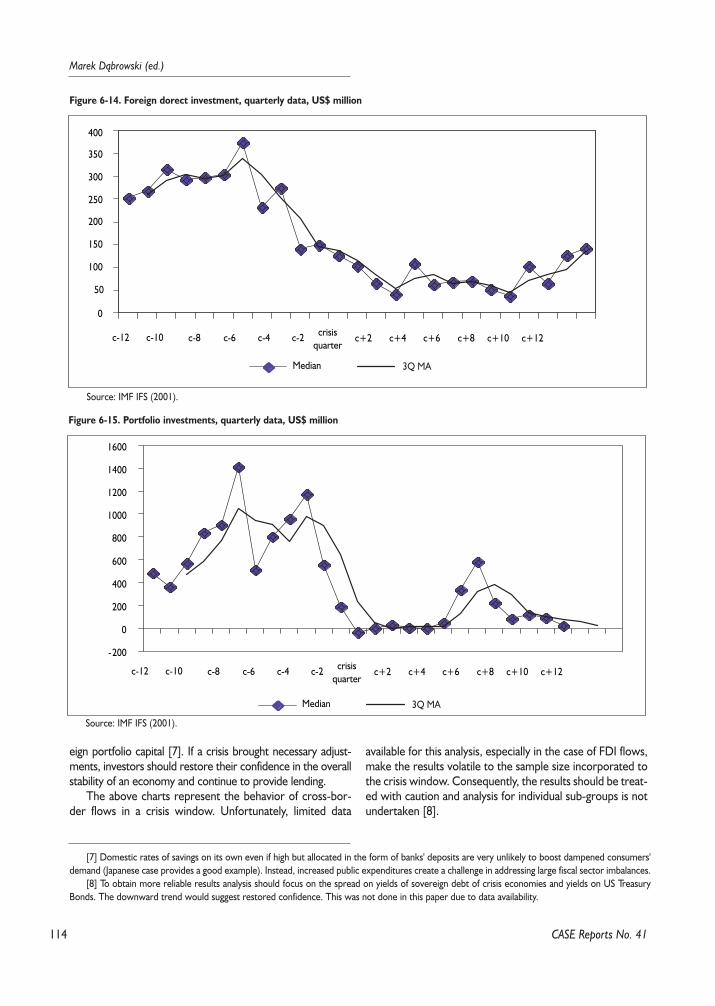
114
Marek D¹browski (ed.)
eign portfolio capital [7]. If a crisis brought necessary adjust-ments, investors should restore their confidence in the overallstability of an economy and continue to provide lending.
The above charts represent the behavior of cross-bor-der flows in a crisis window. Unfortunately, limited data
available for this analysis, especially in the case of FDI flows,make the results volatile to the sample size incorporated tothe crisis window. Consequently, the results should be treat-ed with caution and analysis for individual sub-groups is notundertaken [8].
CASE Reports No. 41
[7] Domestic rates of savings on its own even if high but allocated in the form of banks' deposits are very unlikely to boost dampened consumers'demand (Japanese case provides a good example). Instead, increased public expenditures create a challenge in addressing large fiscal sector imbalances.
[8] To obtain more reliable results analysis should focus on the spread on yields of sovereign debt of crisis economies and yields on US TreasuryBonds. The downward trend would suggest restored confidence. This was not done in this paper due to data availability.
Figure 6-14. Foreign dorect investment, quarterly data, US$ million
0
50
100
150
200
250
300
350
400
c-12 c-10 c-8 c-6 c-4 c-2 crisisquarter
c+2 c+4 c+6 c+8 c+10 c+12
Median 3Q MA
Source: IMF IFS (2001).
Figure 6-15. Portfolio investments, quarterly data, US$ million
-200
0
200
400
600
800
1000
1200
1400
1600
c-12 c-10 c-8 c-6 c-4 c-2 crisisquarter
c+2 c+4 c+6 c+8 c+10 c+12
Median 3Q MA
Source: IMF IFS (2001).
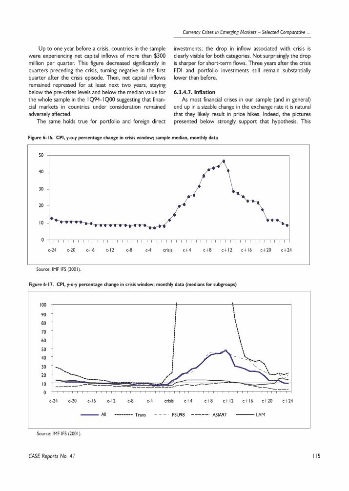
115
Currency Crises in Emerging Markets – Selected Comparative ...
Up to one year before a crisis, countries in the samplewere experiencing net capital inflows of more than $300million per quarter. This figure decreased significantly inquarters preceding the crisis, turning negative in the firstquarter after the crisis episode. Then, net capital inflowsremained repressed for at least next two years, stayingbelow the pre-crises levels and below the median value forthe whole sample in the 1Q94-1Q00 suggesting that finan-cial markets in countries under consideration remainedadversely affected.
The same holds true for portfolio and foreign direct
investments; the drop in inflow associated with crisis isclearly visible for both categories. Not surprisingly the dropis sharper for short-term flows. Three years after the crisisFDI and portfolio investments still remain substantiallylower than before.
6.3.4.7. InflationAs most financial crises in our sample (and in general)
end up in a sizable change in the exchange rate it is naturalthat they likely result in price hikes. Indeed, the picturespresented below strongly support that hypothesis. This
CASE Reports No. 41
Figure 6-16. CPI, y-o-y percentage change in crisis window; sample median, monthly data
0
10
20
30
40
50
c-24 c-20 c-16 c-12 c-8 c-4 crisis c+4 c+8 c+12 c+16 c+20 c+24
Source: IMF IFS (2001).
Figure 6-17. CPI, y-o-y percentage change in crisis window; monthly data (medians for subgroups)
0
10
20
30
40
50
60
70
80
90
Trans FSU98 ASIA97
100
LAMAll
c-24 c-20 c-16 c-12 c-8 c-4 crisis c+4 c+8 c+12 c+16 c+20 c+24
Source: IMF IFS (2001).
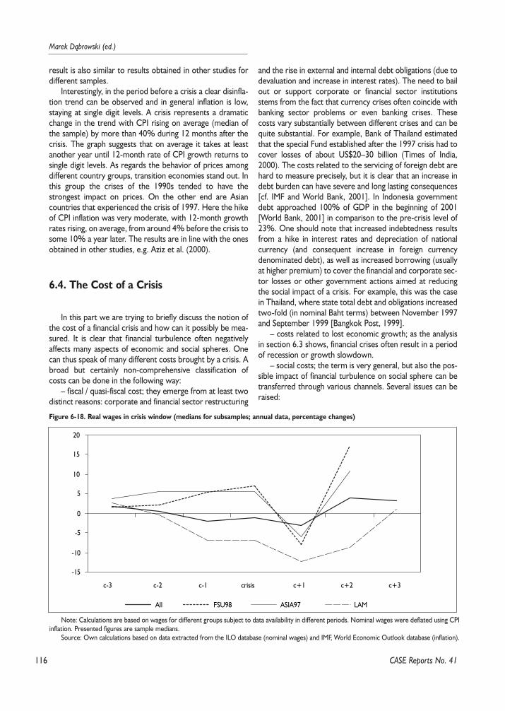
116
Marek D¹browski (ed.)
result is also similar to results obtained in other studies fordifferent samples.
Interestingly, in the period before a crisis a clear disinfla-tion trend can be observed and in general inflation is low,staying at single digit levels. A crisis represents a dramaticchange in the trend with CPI rising on average (median ofthe sample) by more than 40% during 12 months after thecrisis. The graph suggests that on average it takes at leastanother year until 12-month rate of CPI growth returns tosingle digit levels. As regards the behavior of prices amongdifferent country groups, transition economies stand out. Inthis group the crises of the 1990s tended to have thestrongest impact on prices. On the other end are Asiancountries that experienced the crisis of 1997. Here the hikeof CPI inflation was very moderate, with 12-month growthrates rising, on average, from around 4% before the crisis tosome 10% a year later. The results are in line with the onesobtained in other studies, e.g. Aziz et al. (2000).
6.4. The Cost of a Crisis
In this part we are trying to briefly discuss the notion ofthe cost of a financial crisis and how can it possibly be mea-sured. It is clear that financial turbulence often negativelyaffects many aspects of economic and social spheres. Onecan thus speak of many different costs brought by a crisis. Abroad but certainly non-comprehensive classification ofcosts can be done in the following way:
– fiscal / quasi-fiscal cost; they emerge from at least twodistinct reasons: corporate and financial sector restructuring
and the rise in external and internal debt obligations (due todevaluation and increase in interest rates). The need to bailout or support corporate or financial sector institutionsstems from the fact that currency crises often coincide withbanking sector problems or even banking crises. Thesecosts vary substantially between different crises and can bequite substantial. For example, Bank of Thailand estimatedthat the special Fund established after the 1997 crisis had tocover losses of about US$20–30 billion (Times of India,2000). The costs related to the servicing of foreign debt arehard to measure precisely, but it is clear that an increase indebt burden can have severe and long lasting consequences[cf. IMF and World Bank, 2001]. In Indonesia governmentdebt approached 100% of GDP in the beginning of 2001[World Bank, 2001] in comparison to the pre-crisis level of23%. One should note that increased indebtedness resultsfrom a hike in interest rates and depreciation of nationalcurrency (and consequent increase in foreign currencydenominated debt), as well as increased borrowing (usuallyat higher premium) to cover the financial and corporate sec-tor losses or other government actions aimed at reducingthe social impact of a crisis. For example, this was the casein Thailand, where state total debt and obligations increasedtwo-fold (in nominal Baht terms) between November 1997and September 1999 [Bangkok Post, 1999].
– costs related to lost economic growth; as the analysisin section 6.3 shows, financial crises often result in a periodof recession or growth slowdown.
– social costs; the term is very general, but also the pos-sible impact of financial turbulence on social sphere can betransferred through various channels. Several issues can beraised:
CASE Reports No. 41
Figure 6-18. Real wages in crisis window (medians for subsamples; annual data, percentage changes)
-15
-10
-5
0
5
10
15
20
All FSU98 ASIA97 LAM
c-3 c-2 c-1 crisis c+1 c+2 c+3
Note: Calculations are based on wages for different groups subject to data availability in different periods. Nominal wages were deflated using CPIinflation. Presented figures are sample medians.
Source: Own calculations based on data extracted from the ILO database (nominal wages) and IMF, World Economic Outlook database (inflation).
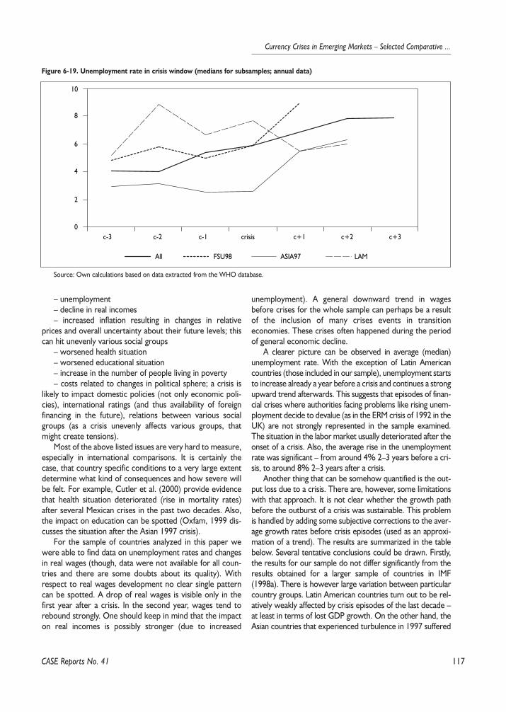
117
Currency Crises in Emerging Markets – Selected Comparative ...
CASE Reports No. 41
– unemployment– decline in real incomes– increased inflation resulting in changes in relative
prices and overall uncertainty about their future levels; thiscan hit unevenly various social groups
– worsened health situation– worsened educational situation– increase in the number of people living in poverty– costs related to changes in political sphere; a crisis is
likely to impact domestic policies (not only economic poli-cies), international ratings (and thus availability of foreignfinancing in the future), relations between various socialgroups (as a crisis unevenly affects various groups, thatmight create tensions).
Most of the above listed issues are very hard to measure,especially in international comparisons. It is certainly thecase, that country specific conditions to a very large extentdetermine what kind of consequences and how severe willbe felt. For example, Cutler et al. (2000) provide evidencethat health situation deteriorated (rise in mortality rates)after several Mexican crises in the past two decades. Also,the impact on education can be spotted (Oxfam, 1999 dis-cusses the situation after the Asian 1997 crisis).
For the sample of countries analyzed in this paper wewere able to find data on unemployment rates and changesin real wages (though, data were not available for all coun-tries and there are some doubts about its quality). Withrespect to real wages development no clear single patterncan be spotted. A drop of real wages is visible only in thefirst year after a crisis. In the second year, wages tend torebound strongly. One should keep in mind that the impacton real incomes is possibly stronger (due to increased
unemployment). A general downward trend in wagesbefore crises for the whole sample can perhaps be a resultof the inclusion of many crises events in transitioneconomies. These crises often happened during the periodof general economic decline.
A clearer picture can be observed in average (median)unemployment rate. With the exception of Latin Americancountries (those included in our sample), unemployment startsto increase already a year before a crisis and continues a strongupward trend afterwards. This suggests that episodes of finan-cial crises where authorities facing problems like rising unem-ployment decide to devalue (as in the ERM crisis of 1992 in theUK) are not strongly represented in the sample examined.The situation in the labor market usually deteriorated after theonset of a crisis. Also, the average rise in the unemploymentrate was significant – from around 4% 2–3 years before a cri-sis, to around 8% 2–3 years after a crisis.
Another thing that can be somehow quantified is the out-put loss due to a crisis. There are, however, some limitationswith that approach. It is not clear whether the growth pathbefore the outburst of a crisis was sustainable. This problemis handled by adding some subjective corrections to the aver-age growth rates before crisis episodes (used as an approxi-mation of a trend). The results are summarized in the tablebelow. Several tentative conclusions could be drawn. Firstly,the results for our sample do not differ significantly from theresults obtained for a larger sample of countries in IMF(1998a). There is however large variation between particularcountry groups. Latin American countries turn out to be rel-atively weakly affected by crisis episodes of the last decade –at least in terms of lost GDP growth. On the other hand, theAsian countries that experienced turbulence in 1997 suffered
Figure 6-19. Unemployment rate in crisis window (medians for subsamples; annual data)
0
2
4
6
8
10
All FSU98 ASIA97 LAM
c-3 c-2 c-1 crisis c+1 c+2 c+3
Source: Own calculations based on data extracted from the WHO database.
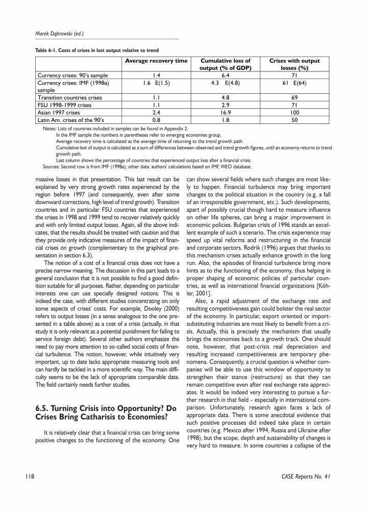
118
Marek D¹browski (ed.)
massive losses in that presentation. This last result can beexplained by very strong growth rates experienced by theregion before 1997 (and consequently, even after somedownward corrections, high level of trend growth). Transitioncountries and in particular FSU countries that experiencedthe crises in 1998 and 1999 tend to recover relatively quicklyand with only limited output losses. Again, all the above indi-cates, that the results should be treated with caution and thatthey provide only indicative measures of the impact of finan-cial crises on growth (complementary to the graphical pre-sentation in section 6.3).
The notion of a cost of a financial crisis does not have aprecise narrow meaning. The discussion in this part leads to ageneral conclusion that it is not possible to find a good defin-ition suitable for all purposes. Rather, depending on particularinterests one can use specially designed notions. This isindeed the case, with different studies concentrating on onlysome aspects of crises' costs. For example, Dooley (2000)refers to output losses (in a sense analogous to the one pre-sented in a table above) as a cost of a crisis (actually, in thatstudy it is only relevant as a potential punishment for failing toservice foreign debt). Several other authors emphasize theneed to pay more attention to so-called social costs of finan-cial turbulence. The notion, however, while intuitively veryimportant, up to date lacks appropriate measuring tools andcan hardly be tackled in a more scientific way. The main diffi-culty seems to be the lack of appropriate comparable data.The field certainly needs further studies.
6.5. Turning Crisis into Opportunity? DoCrises Bring Catharisis to Economies?
It is relatively clear that a financial crisis can bring somepositive changes to the functioning of the economy. One
can show several fields where such changes are most like-ly to happen. Financial turbulence may bring importantchanges to the political situation in the country (e.g. a fallof an irresponsible government, etc.). Such developments,apart of possibly crucial though hard to measure influenceon other life spheres, can bring a major improvement ineconomic policies. Bulgarian crisis of 1996 stands an excel-lent example of such a scenario. The crisis experience mayspeed up vital reforms and restructuring in the financialand corporate sectors. Rodrik (1996) argues that thanks tothis mechanism crises actually enhance growth in the longrun. Also, the episodes of financial turbulence bring morehints as to the functioning of the economy, thus helping inproper shaping of economic policies of particular coun-tries, as well as international financial organizations [Köh-ler, 2001].
Also, a rapid adjustment of the exchange rate andresulting competitiveness gain could bolster the real sectorof the economy. In particular, export oriented or import-substituting industries are most likely to benefit from a cri-sis. Actually, this is precisely the mechanism that usuallybrings the economies back to a growth track. One shouldnote, however, that post-crisis real depreciation andresulting increased competitiveness are temporary phe-nomena. Consequently, a crucial question is whether com-panies will be able to use this window of opportunity tostrengthen their stance (restructure) so that they canremain competitive even after real exchange rate appreci-ates. It would be indeed very interesting to pursue a fur-ther research in that field – especially in international com-parison. Unfortunately, research again faces a lack ofappropriate data. There is some anecdotal evidence thatsuch positive processes did indeed take place in certaincountries (e.g. Mexico after 1994, Russia and Ukraine after1998), but the scope, depth and sustainability of changes isvery hard to measure. In some countries a collapse of the
CASE Reports No. 41
Table 6-1. Costs of crises in lost output relative to trend
Average recovery time Cumulative loss ofoutput (% of GDP)
Crises with outputlosses (%)
Currency crises: 90’s sample 1.4 6.4 71Currency crises: IMF (1998a)sample
1.6 E(1.5) 4.3 E(4.8) 61 E(64)
Transition countries crises 1.1 4.8 69FSU 1998-1999 crises 1.1 2.9 71Asian 1997 crises 2.4 16.9 100Latin Am. crises of the 90’s 0.8 1.8 50
Notes: Lists of countries included in samples can be found in Appendix 2.In the IMF sample the numbers in parentheses refer to emerging economies group.Average recovery time is calculated as the average time of returning to the trend growth path.Cumulative lost of output is calculated as a sum of differences between observed and trend growth figures, until an economy returns to trend growth path.Last column shows the percentage of countries that experienced output loss after a financial crisis.
Sources: Second row is from IMF (1998a); other data: authors' calculations based on IMF, WEO database.

119
Currency Crises in Emerging Markets – Selected Comparative ...
exchange rate can be seen as a mechanism removing exist-ing imbalances, while not being able to impel significantpositive internal changes. There is clearly much variationbetween countries.
The impact on economic policies and, in particular, onthe will and ability of the authorities to pursue difficultreforms is perhaps one of the most important topics ofstudy in transition countries. It is, however, a very difficulttask and certainly lies beyond the scope of this paper. Wecan only make a few points at this stage.
Financial crises can be seen as mechanisms of rapidadjustment and bringing economies back to balance. Cer-tainly, such an approach does not capture all kinds of crises(as allegedly they may also result from speculative attackwhen there are no fundamental imbalances). If oneaccepts such a view, the next question naturally arises, ofwhether the change brought by a crisis is sustainable. Inother words, it is very important to see whether crisestend to permanently (i.e. for a long time) remove underly-ing imbalances. Again, approaching such a question ininternational comparison is quite difficult. One obviousreason is that it is usually quite hard to recognize theunderlying causes of any particular crisis, not to mention alarge sample of crises. One thing that could be done is tocheck the behavior of some standard indicators that arecommonly thought to be likely associated with financialturbulence. The discussion of various crisis indicators canbe found e.g. in Tomczyñska (2001), Kaminsky et al.(1998).
The idea is to check whether any particular indicatorwas indeed observed before a crisis (interpreted as pres-ence of some fundamental problems in related spheres)and then to check whether the situation improved after acrisis. Due to data limitations it was only possible to dosuch an exercise for current account deficit (a survey of lit-erature dealing with the role of current account deficits inprovoking financial crises can be found, e.g. in Sasin,2001). The table below presents the outcome of the fol-lowing procedure. The current account balance relative toGDP (in percent) was studied in three years preceding andthree years following a crisis year. A 'problem' with currentaccount imbalance was defined as deficit larger than 4% ofGDP in any two of the three preceding years or deficit ofmore than 6% of GDP in a year before a crisis. A currentaccount 'problem' after a crisis was defined in a similarway: deficit larger than 4% of GDP in any two of the three
following years or deficit larger than 6% of GDP in thethird year after a crisis. Such a threshold allowed for iden-tifying of 13 crises where current account was potentiallya problem beforehand. Of these, in 9 cases the situationimproved and current account deficits were reduced (orturned into surpluses) in three years after crises, while in4 cases there was no much improvement. Additionally, in5 cases, the current account deficits widened significantlyafter financial turbulence, while the model signaled noproblems before a crisis. Also, the data are not alwaysavailable for all three years after crises, so the statisticsmight actually look even worse. The general conclusionfrom that exercise is that financial crises in our samplewere quite varied phenomena in terms of current accountposition. Consequently, for some countries, potentialimbalances were removed by a crisis, while for the otherthey remained in place or even newly emerged.
6.6. Conclusions
The review of literature carried in section two showsthat there is a substantial gap in existing writing on theconsequences of financial crises. In particular, transitioncountries are rarely included in cross-country studies.Also, due to data limitations, analyses attempting interna-tional comparisons usually not include the most recent cri-sis episodes, i.e. the Asian crises of 1997 and FSU crises of1998 and 1999.
This paper tries to contribute its part in research onthe various outcomes that are brought by financial turbu-lence. In particular, an attempt is made to assess the per-formance of transition economies in this respect and toinclude the newest available data, so that the analysis cancover the crises that emerged in 1997–1999.
The results of graphical presentations carried in sec-tion three remain broadly in line with other similar studies.In some instances there is large variation in outcomes ofcrises in different sub-groups. The available data do notallow, however, for concluding that the crises of the lastdecade or the crises in transition economies – in terms oftheir consequences – differ from other financial crashes.As for output trends, the general finding is that, on aver-age, after the sharp drop in a crisis year, GDP growthrecovers gradually and starting from the second year after
CASE Reports No. 41
Table 6-2. Current account position before and after a crisis
Large CA deficitbefore a crisis
‘Safe’ CA positionbefore a crisis
Large CA deficit aftera crisis
‘Safe’ CA positionafter a crisis
No data after a crisis
13 4 916 5 8 3
Note: See text for more explanation.Source: Own calculation based on IMF data (IFS for current account, WEO for GDP).
120
Marek D¹browski (ed.)
a crisis the rebound speeds up. Yet, available data do notallow for stating whether this increase may be maintainedin a longer run. Also, taking a look at the development ofparticular components of GDP for the whole sample, aworrying factor is decelerating rate of investments alreadyin the third year after a crisis (following a reboundobserved in the second year). Another interesting obser-vation is that net capital inflows remain depressed for along time after crises not reaching pre-crisis highs. Thisfactor also suggests that the recovery may prove weak.
The evidence presented in this paper, although limitedby the data availability, shows that various costs associatedwith financial crises are on average indeed high. A medianof crises included in the sample led to a significant loss ofoutput, increase in unemployment and also a fall in realwages. There are also many other negative consequences,such as sizable fiscal costs, deteriorating social stance, etc.
With respect to the positive outcomes of financial tur-bulence incidents, in some cases they provided stimulusfor a change in economic policies and speeding up reforms.However, often too, post-crises reforms proceed slowlybecause they are subject to social constraints and politicalpressures. Lower growth in the aftermath of a crisis doesnot help to overcome these problems. For example, inSoutheast Asia restructuring process still remains in direstraits. Political tensions, if present, are unlikely to beremoved by a crisis with Indonesia being an excellentexample. The real sector, especially export orientedbranches, benefit from increased competitiveness(although the data on export performance does not allowfor making strong statistical inference). The simple exer-cise was carried in order to check whether crises are ableto remove existing imbalances in the economies, thusreducing a threat of crisis reappearance. It proved thatwhile this seems to be the case in some instances; in gen-eral, this cannot be demonstrated (the analysis was carriedfor current account balances).
Certainly, the scope for further research remains vast.The experience of this paper shows that it is necessary tostrengthen the available databases that would allow a moreappropriate analysis of crises' impact, especially in thesocial sphere. Also, the influence on economic policies andinstitutions in crisis affected countries remains as a verypromising and very important (due to its bearing on devel-opment) field for further research.
Appendix. The Definition of a Crisis
The pressure index that we use in order to identify cri-sis episodes is defined as follows:
EMPC,T = αC [(eC,T / eC,T-1) -1] - β [(rC,T / rC,T-1) -1] + γ[(iC,T / iC,T-1) -1]
CrisisC,T =1 if EMPC,T > δ ∗ σEMP + µEMP=0 otherwise,
EMP – exchange market pressure index,e – exchange rate (domestic currency vs. US dollar),i – domestic nominal interest rate,r – reserves,C – country T – timeα, β, γ, δ – weights,δEMP – the sample standard deviationµEMP – the sample mean
Appendix 2. The List of CountriesIncluded in the Analysis
ALBANIA, ARGENTINA, ARMENIA, AZERBAIJAN,BELARUS, BOLIVIA, BRAZIL, BULGARIA, CHILE,CHINA, HONG KONG, CROATIA, CZECH REPUBLIC,ESTONIA, GEORGIA, HUNGARY, INDIA, INDONESIA,KAZAKHSTAN, KOREA, KYRGYZ REPUBLIC, LATVIA,LITHUANIA, MACEDONIA, MALAYSIA, MEXICO,MOLDOVA, PHILIPPINES, RUSSIA, SINGAPORE, SLO-VAK REPUBLIC, SLOVENIA, SRI LANKA, TAIWAN,TAJIKISTAN, THAILAND, TURKEY, TURKMENISTAN,UKRAINE, UZBEKISTAN, VENEZUELA.
Within the whole sample, the following sub-sampleswere identified:
Transition economies (TE): ALBANIA, ARMENIA,AZERBAIJAN, BELARUS, BULGARIA, CROATIA, CZECHREPUBLIC, ESTONIA, GEORGIA, HUNGARY, KAZA-KHSTAN, KYRGYZ REPUBLIC, LATVIA, LITHUANIA,MACEDONIA, MOLDOVA, RUSSIA, SLOVAK REPUBLIC,SLOVENIA, TAJIKISTAN, TURKMENISTAN, UKRAINE,UZBEKISTAN.
FSU countries that underwent a crisis in 1998/99 (FSU98): BELARUS, GEORGIA, KAZAKHSTAN, KYRGYZREPUBLIC, RUSSIA, UKRAINE.
Southeast Asian economies that underwent a crisis in1997 (ASIA97): INDONESIA, KOREA, MALAYSIA,PHILIPPINES, THAILAND.
Latin American economies (LAM): ARGENTINA,BOLIVIA, BRAZIL, CHILE, MEXICO, VENEZUELA.
CASE Reports No. 41

121
Currency Crises in Emerging Markets – Selected Comparative ...
References
Aizenman J. (1998). "Volatility and Welfare Costs ofFinancial Market Integration". NBER WP 6782.
Alesina A. (1989). "Why are Stabilizations Delayed?".NBER WP 3053.
Aziz Jahangir et al. (2000). "Currency Crises: In Searchof Common Element". IMF Working Paper WP/00/67.
Bangkok Post (1999). "Economic Review 1999". Year-end Edition, web page: www.bangkokpost.net/99year-end/
Bernanke B.S., M. Gertler (1995). "Inside the BlackBox: The Credit Channel of Monetary Transmission". Jour-nal of Economics Perspective, 24–48.
Berry S. et al. (1999). "Impact of the Indonesian Crisis:Price Changes and the Poor". NBER WP 7194.
Bordo M.D., A.J. Schwartz (1999). "Under What Cir-cumstances, Past and Present, Have International Rescuesof Countries in Financial Distress Been Successful?". Jour-nal of International Money and Finance 18, pp. 683–708.
Bordo M.D., A.J. Schwartz (2000). "Measuring RealEconomic Effects of Bailouts: Historical Perspective onHow Countries in Financial Distress Have Fared With andWithout Bailouts". NBER WP 7701.
Bustelo P. (1998). "The East Asian Financial Crises: AnAnalytical Survey". ICEI Working Paper 10/1998, web pagewww.ucm.es
CEMAIP (1998). "Report on the World Monetary andFinancial Crises and Their Effects on the Economy of theEuropean Union". Committee on Economic and MonetaryAffairs and Industrial Policy, web site: http://attac/org/fra
Cutler D.M. et al. (2000). "Financial Crisis, Health Out-comes and Aging: Mexico in the 1980s and 1990s". NBERWorking Paper 7746.
Dooley M.P. (2000). "Can Output Losses FollowingInternational Financial Cries be Avoided?". NBER WorkingPaper 7531.
Eichengreen B., A.K. Rose, Ch. Wyplosz (1996). "Con-tagious Currency Crises". NBER WP No 5681.
Ferri G. (1998). "The Real Impact of Financial Shocks:Evidence from the Republic of Korea". World Bank Work-ing Papers.
Flood R., N. Marion (1998). "Perspectives on theRecent Currency Crisis Literature", NBER, WP 6380.
Forbes K. (2000). "The Asian Flu and Russian Virus:Firm-Level Evidence on How Crises are Transmitted Inter-nationally". NBER WP 7807.
Frankel J., A. Rose (1996). "Currency Crashes inEmerging Markets: Empirical Indicators". CEPR DiscussionPaper, No 1349.
Grupta, et al. (1998). "Mitigating the Social Costs of theEconomic Crisis and the Reform Program in Asia". IMFPaper on Policy Analysis an Assessment.
ILO (1998). "The Social Impact of the Asian FinancialCrisis". Technical report, web page: www.ilo.org
IMF (1998a). "World Economic Outlook". (May). Finan-cial Crises: Causes and Indicators.
IMF (1998b). "World Economic Outlook". (October).Financial Turbulence and the World Economy.
IMF (1999). "World Economic Outlook". (May).IMF and World Bank (2001). "Armenia, Georgia, Kyr-
gyz Republic, Moldova, and Tajikistan: External Debt andFiscal Sustainability".
Jones S. (1998). "Social Cost of Asian Crisis". FinancialTimes, January 26.
Kakwani N., N. Prescott (1999). "Impact of EconomicCrisis on Poverty and Inequality in Korea". Processed.World Bank, Washington, D.C.
Kaminsky G., S. Lizondo, C.M. Reinhard (1997). "Lead-ing Indicators of Currency Crises". IMF WP No. 97/79.
Kindleberger Ch.P. (2000). "Maniacs, Panics, andCrashes: A History of Financial Crashes". John Wiley &Sons.
Köhler H. (2001). "Home Free? Turning Crisis intoOpportunity". Asian Wall Street Journal, January 8.
Manuelyan et al. (2000). "Special Focus: Poverty Dur-ing Crisis and Recovery". web site: www.worldbank.org
Milesi-Ferretti G.M., A. Razin (1998). "CurrentAccount Reversals and Currency Crises: Empirical Regu-larities". IMF WP No. 98/89.
Mishkin F. S. (1996). "The Channels of Monetary Trans-mission: Lessons for Monetary Policy". NBER WorkingPaper, No. W5464.
Oxfam (1999). "Education Now: Break the Cycle ofPoverty". web page: http://www.caa.org.au/oxfam/
Rodrik D. (1996). "Understanding Economic PolicyReform". Journal of Economic Literature, Vol. 34 pp. 9–41,March.
Rodrik D. (1998). "Where Did All the Growth Go?External Shocks, Social Conflict, and Growth Collapses".NBER Working Paper No. 6350.
Sasin M. (2001). "The Importance of the Real ExchangeRate Overvaluation and the Current Account Deficit in theEmergence of Financial Crises". CASE Reports No. 41.
Stiglitz J. (1998). "Must Financial Crises Be This Fre-quent and This Painful?". McKay Lecture (Pittsburgh, Penn-sylvania).
Szczurek M. (2001). "International Liquidity and theCost of Currency Crises". CASE Reports No. 41.
The Times of India (2000). "Thai financial crisis cost upto $30.8 bn". 24 May.
Tomczyñska M. (2000). "Early Indicators of CurrencyCrises". Review of some literature, CASE Studies & Analy-ses No.208
UN (1999). "World Economic and Social Survey". 1999,UN web site
CASE Reports No. 41
122
Marek D¹browski (ed.)
Westin P. (1999). "One Year After the Crisis: WhatWent Right?". Russian Economic Trends, September.
World Bank (2001). "East Asia Update. RegionalOverview". March, web page: www.worldbank.org
CASE Reports No. 41

123
Currency Crises in Emerging Markets – Selected Comparative ...
CASE Reports No. 41
7.1. Introduction
The IMF has supported the transition process in anumber of FSU countries. This support involved conces-sionary financing, policy advice and technical assistance.Notwithstanding temporary conflicts, the cooperationbetween the Fund and FSU countries throughout the peri-od was described by the Fund as generally successful. Itwas argued that it contributed to the macroeconomic andfinancial stabilization [1]. Yet, the financial crisis of 1998wiped out this stabilization and proved that previous poli-cies were fully unsustainable. This paper attempts toanswer the crucial question why countries collaboratingclosely with the IMF and implementing policies supportedby the Fund had to undergo deep financial crisis. The ques-tion is made more intriguing by earlier research [2] show-ing that this was a first-generation crisis – that is, onecaused by bad policies that led to macroeconomic imbal-ances. While the core of the problems was domestic,deterioration of external conditions was the trigger thatstarted the inevitable collapse. True, it is also well under-stood now that vested interests, insufficient structuralreforms and lack of political were crucial factors prevent-ing necessary policy adjustments. But has the Fund influ-enced the pace of structural reforms and fiscal tightening?Should the IMF have been more insistent on reformsthrough tighter conditionality or have allowed for morereform ownership? Finally, should it have withdrawn longbefore 1998 and not underwritten unsustainable policies?
Before we proceed with addressing these questions wewould like to make a short comment on the methodology.In order to evaluate the impact of the IMF program on theeconomic situation we have to distinguish some specific
questions. First, the original design of the program (assump-tions and targets) and its adequacy for the economic prob-lems of the countries under investigation are discussed. Sec-ond, the implementation of the program is evaluated, espe-cially the compliance with the performance criteria. Third,if the IMF chooses to support the program even thoughsome of its key parameters are breached, we conclude thatthe Fund is still sharing ownership for the final outcome.One of the advantages of case studies, as opposed to largemulti-country studies [3], is the ability not only to test thesignificance of the sheer existence of the program but alsoto better evaluate its key parameters and consider the qual-ity of its implementation. At the same time we believe thatthe group of countries under investigation – Russia,Ukraine, Moldova, Georgia and Kyrgyzstan (RUMGK) – islarge and diversified enough to allow for some generaliza-tion of results.
There is also a problem of the baseline scenario againstwhich one can compare the outcome of IMF-supportedprograms. In the literature [4] there are three majorapproaches. The before and after approach simply com-pares the situation in the country before and after theadoption of the IMF-supported programs. This approach isimperfect especially if the country has faced an importantexogenous shock or had to undertake fundamentalchanges in its economic structure. For that reason, thisapproach is not suitable for the evaluation of programs intransition economies. Another popular approach is tocompare countries that adopted the IMF program withcountries of similar characteristics (in terms of economicstructures and exposure to external shocks) that did not.In the case of FSU countries there is no such control groupas virtually all transition countries cooperated with theIMF [5]. The only theoretically reliable method of assess-ing the impact of this program is based on the construction
Part VII.Financial Crises in FSU Countries: The Role of the IMFRafa³ Antczak, Ma³gorzata Markiewicz, Artur Radziwi³³
[1] The large majority of IMF documents related to programs in transition economies (at least until the 1998 crisis) began and concluded with thepraise of stabilization achievements and progress in structural reforms. Compare: IMF (MEP, LI, A4C, RED, SP), Camdessus (1994) and Fischer (1998).
[2] Compare country monographs prepared under this project: Antczak (2000), Markiewicz (2000) and Radziwill (2000), and also: Siwinska (2000).[3] See Haque and Khan (1998) for discussion.[4] Ibid.[5] Among 26 transition countries, only Turkmenistan did not have at least one IMF-supported program.

124
Marek D¹browski (ed.)
CASE Reports No. 41
of the counterfactual scenario: "comparing the macroeco-nomic outcomes of a program with the corresponding out-comes obtained under an alternative set of feasible policiesis the most appropriate way of judging the effects of pro-grams. However, the difficulties involved in using this cri-teria should not be underestimated" [6]. Actually thisapproach is especially difficult in the case of transitioncountries. With a newly emerging and constantly changingstructure of the economy, it is impossible to build a fullstructural model of the economy. However, throughoutthe discussion of the political economy of reforms andmoral hazard we cannot avoid asking "what if…". The lastmethodological point is more trivial and relates to scarci-ties of data. As details of program arrangements, at leastuntil 1998, were generally confidential, it was "extremelydifficult for outside observers to prepare a serious quanti-tative analysis appraisal of IMF policies" [7]. We try to over-come the problem through extensive use of publishedmaterials and materials released by the governments of thecountries in question.
The remainder of this paper is organized in the followingway. Chapter one presents the character and main causes ofthe financial crisis in FSU countries. Chapter two discusseswhat impact IMF policies could have had in crisis prevention.It also presents the general logic of IMF programs and priorexperience of the Fund that contributed substantially to theway it handled cooperation with transition countries.
Against this background, chapter three describes the designand scale of the IMF programs in the region. Chapter fouridentifies program deficiencies and shows their impact onthe policies. Chapter five concludes by commenting on theinstitutional factors that could have contributed to theseweaknesses.
7.2. The Nature of Financial Crisis in FSUCountries
The existing literature shows clearly that the financialcrisis that affected FSU countries in 1998 can be convinc-ingly explained by fundamental macroeconomic imbal-ances [8]. Loose fiscal policy and the lack of structuralreforms resulted in unsustainable internal and externalpositions. Without rapid policy adjustments, this situationhad to lead to a financial crisis. For Russia the turmoil infinancial markets following the Asian crisis in 1997 com-bined with the falling prices of oil constituted the triggerthat revealed existing imbalances and especially the accu-mulation of debt service liabilities. For other countries, theclear contagion pressures from Russia (operating boththrough the trade and financial market channels) led toopen crisis only in economies with similar fundamentalweaknesses. Among these weaknesses the most easily vis-
Figure 7-1. General government balance (the cash basis), percent of GDP
Russia
Ukraine
Moldova
Georgia
Kyrgyzstan
1992
1993
1994
1995
1996
1997
1998
1999
0
-5
-10
-15
-20
-25
-30
Source: IMF (RED).
[6] Haque and Khan (1998).[7] Jeffrey Sachs, cited in Bandow and Vasquez (1994).[8] Compare footnote 2.

125
Currency Crises in Emerging Markets – Selected Comparative ...
CASE Reports No. 41
ible was a deep fiscal deficit [9]. Fiscal imbalances werepermanently very large in all five countries studied here,with the possible exception of Ukraine, where the deficitwas not above 5 percent of GDP since 1995. Figure 7-1presents deficits on cash basis. If expenditure arrears arealso accounted for, imbalances are even larger.
However, even under fiscal policy that is unsustainable inthe longer run, short-term monetary stabilization can beachieved. This was accomplished by stabilizing exchangerates in Russia, Moldova, Georgia, and Kyrgyzstan beginningin mid-1994, and in Ukraine beginning in mid-1995, and last-ed until the August 1998 crisis. Stable exchange rates were
maintained at the expense of central banks interventions(especially in Russia and Ukraine), while foreign currencyreserves were replenished by disbursements from the IMF.The proceeds from sale of reserves served in turn as asource of budget deficit financing in these two countries.Moldova, Georgia and Kyrgyzstan relied mainly on govern-ment official transfers and contracted foreign debt to sup-port exchange rate stabilization and finance budget deficits.
As a result of exchange rate based stabilizations andexternal sources of deficit financing CPI inflation (and infla-tionary expectations) in RUMGK was lowered to moderatelevels during 1995–1998. Low inflation rates and stable
Figure 7-2. Changes in nominal exchange rates, monthly (1992-1999)
-20
0
20
40
60
80
100
120
Russia Ukraine Kyrgyzstan Moldova Georgia
92M
07
93M
01
93M
07
94M
01
94M
07
95M
01
95M
07
96M
01
96M
07
97M
01
97M
07
98M
01
98M
07
99M
01
99M
07
Source: IMF (IFS).
[9] Dabrowski (1999b) writes "Experience of transition process gives a lot of evidence that fiscal policy performance reflects a quality of econom-ic policy and systemic reforms in the specific country. Any inconsequence of the conducted policy, delay in transition on the microeconomic level, weak-ness of government institutions and favorable political climate for intensive rent seeking negatively influence fiscal balances. Thus fiscal equilibriumdepends not only on the fiscal policy itself but also on the speed, quality, and consequence of overall reform process."
Figure 7-3. CPI inflation rate, end-period (percent)
0
50
100
150
200
250
1995
1996
1997
1998
1999
0
2000
4000
6000
8000
10000
12000
1992
1993
1994
Russia
Ukraine
MoldovaGeorgia
Kyrgyzstan
Source: IMF (RED).
126
Marek D¹browski (ed.)
CASE Reports No. 41
exchange rates also allowed for issuance of treasury papersto residents and non-residents what attracted foreign port-folio investors to finance fiscal deficits.
Changing the pattern of deficit financing was a step in theright direction but was not followed by the hard budget con-straints necessary for the market economy to functionproperly. This inconsistency led to accumulation of highdebt burdens with an unfavorable structure (i.e., a largeshare of short-term liabilities held by non-residents). Theprevailing view at the time was that deficits in transitioncould be accepted as long as they are caused by transitionalexpenditures [10]. However, the primary reasons behindfiscal deficits in the countries under investigation were delayin fiscal reforms and maintenance of pre-transition budget-ing practices, and not the costs of reforms. As a result, addi-tional resources and time were lost: foreign financing wasused for current spending and not for implementing neces-sary reforms [11]. This left the countries extremely vulner-able to change in risk perceptions on international financialmarkets.
7.3. The Role of the IMF
The crises in the region have originated mainly from irre-sponsible fiscal policies. Therefore, the role that the IMFplayed needs to be evaluated on the basis of the impact thatIMF-supported programs had on the fiscal stance. Thisimpact could be made through the following methods forcorrecting imbalances:
– tight performance criteria (ceilings on budget deficits,accumulation of debt and arrears, and financing from centralbanks);
– relevant structural benchmarks related to reform ofthe fiscal sector (tax system, expenditures and their prioriti-zation, budgetary process) and policy advice;
– strict conditionality regarding compliance with perfor-mance criteria and structural benchmarks.
These three interdependent aspects could have enabledgovernments to run restrictive policies, even if the currentpolitical situation created pressure for unsustainable policies.If domestic reformers were prepared to follow the path ofresponsible policies, external binding commitment could givethem an additional political instrument. However, otheraspects of the program have to be taken into account too:
– unrealistic assumptions concerning GDP growth,exports, and budget revenues that led to formulation of pro-
grams that were sustainable only if these assumptions wererealized;
– lax conditionality, undermining macroeconomic disci-pline;
– a lenient approach to accumulation of arrears and debt;– improving access to non-inflationary sources of deficit
financing;– ineffective conditionality in the area of structural
reforms, stimulating "paper reforms" and not real restruc-turing of the economy.
In our view, this group of factors (discussed at lengthlater in this paper) was detrimental to necessary fiscaladjustment and undermined the possible disciplinary effectsoutlined before. This weakness was tightly linked to thechanges in the way the IMF has been operating since thedebt crisis in the beginning of the 1980s.
IMF: evolution prior to transitionOf all international organizations, the IMF played the
most important role in the process of transition of post-communist economies [12] . This is explained by the factthat by the early 1990s the IMF acquired significant experi-ence not only in macroeconomic policy but also in structur-al and institutional reform. It was, therefore, perceived asfully prepared to assume responsibility to monitor, manage,and support the transformation process in the mediumterm. But all these activities were quite different from thetasks for which the IMF was originally designed for.
The IMF was established in 1946 as the part of the Bret-ton Woods system. The Fund's role was to provide short-term financing to countries with balance of payment prob-lems in order to avoid the repetition of interwar protec-tionist practices and competitive devaluations. The IMF hada systemic role in supporting the global exchange rate sys-tem. Accordingly, it worked mainly with developed coun-tries and its focus was constrained to the main monetaryand fiscal aggregates. Structural policies were largely absentin IMF-supported programs and the importance of condi-tionality was rather weak. Conditionality was formallyadded to the Articles of Agreement only in 1968 and untilthe mid-1970s included only macroeconomic aggregates.However, after 1971, in the aftermath of the collapse ofBretton Woods system, the IMF lost its core task. Floatingexchange rate regimes among most developed countries didnot require constant surveillance and support from theFund. As Milton Friedman put it [13]: "the IMF has lost itsonly function and should have closed shop". Instead, in the1970s the scope of Fund's activities started to move increas-ingly towards cooperation with developing countries. The
[10] Compare Sachs (1994). For the contrary view see: Dabrowski (1995).[11] Dabrowski (1999a).[12] Dabrowski (1995) and Gomulka (1995).[13] Friedman (1998).
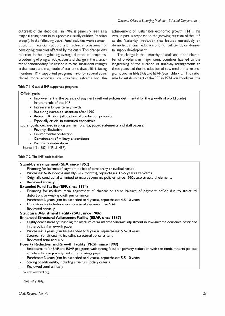
127
Currency Crises in Emerging Markets – Selected Comparative ...
outbreak of the debt crisis in 1982 is generally seen as amajor turning point in this process (usually dubbed "missioncreep"). In the following years, Fund activities were concen-trated on financial support and technical assistance fordeveloping countries affected by the crisis. This change wasreflected in the lengthening average duration of programs,broadening of program objectives and change in the charac-ter of conditionality. "In response to the substantial changesin the nature and magnitude of economic disequilibria facingmembers, IMF-supported programs have for several yearsplaced more emphasis on structural reforms and the
achievement of sustainable economic growth" [14]. Thiswas, in part, a response to the growing criticism of the IMFas the "austerity" institution that focused excessively ondomestic demand reduction and not sufficiently on domes-tic supply development.
The change in the hierarchy of goals and in the charac-ter of problems in major client countries has led to thelengthening of the duration of stand-by arrangements tothree years and the introduction of new medium-term pro-grams such as EFF, SAF, and ESAF (see Table 7-2). The ratio-nale for establishment of the EFF in 1974 was to address the
CASE Reports No. 41
Table 7-1. Goals of IMF-supported programs
Official goals:• Improvement in the balance of payment (without policies detrimental for the growth of world trade)- Inherent role of the IMF• Increase in longer term growth- Receiving increased attention after 1982• Better utilization (allocation) of production potential- Especially crucial in transition economies
Other goals, declared in program memoranda, public statements and staff papers:- Poverty alleviation- Environmental protection- Containment of military expenditure- Political considerations
Source: IMF (1987), IMF (LI, MEP).
[14] IMF (1987).
Table 7-2. The IMF basic facilities
Stand-by arrangement (SBA, since 1952)- Financing for balance of payment deficit of temporary or cyclical nature- Purchases: 6-36 months (initially 6-12 months), repurchases 3.5-5 years afterwards- Originally conditionality limited to macroeconomic policies, since 1980s also structural elements- Reviewed annuallyExtended Fund Facility (EFF, since 1974)- Financing for medium term adjustment of chronic or acute balance of payment deficit due to structural
distortions or weak growth performance- Purchases: 3 years (can be extended to 4 years), repurchases: 4.5-10 years- Conditionality includes more structural elements than SBA- Reviewed annuallyStructural Adjustment Facility (SAF, since 1986)Enhanced Structural Adjustment Facility (ESAF, since 1987)- Highly concessionary financing for medium-term macroeconomic adjustment in low–income countries described
in the policy framework paper- Purchases: 3 years (can be extended to 4 years), repurchases: 5.5-10 years- Stronger conditionality, including structural policy criteria- Reviewed semi-annuallyPoverty Reduction and Growth Facility (PRGF, since 1999)- Replacement for SAF and ESAF programs with strong focus on poverty reduction with the medium term policies
stipulated in the poverty reduction strategy paper- Purchases: 3 years (can be extended to 4 years), repurchases: 5.5-10 years- Strong conditionality, including structural policy criteria- Reviewed semi-annually
Source: www.imf.org.
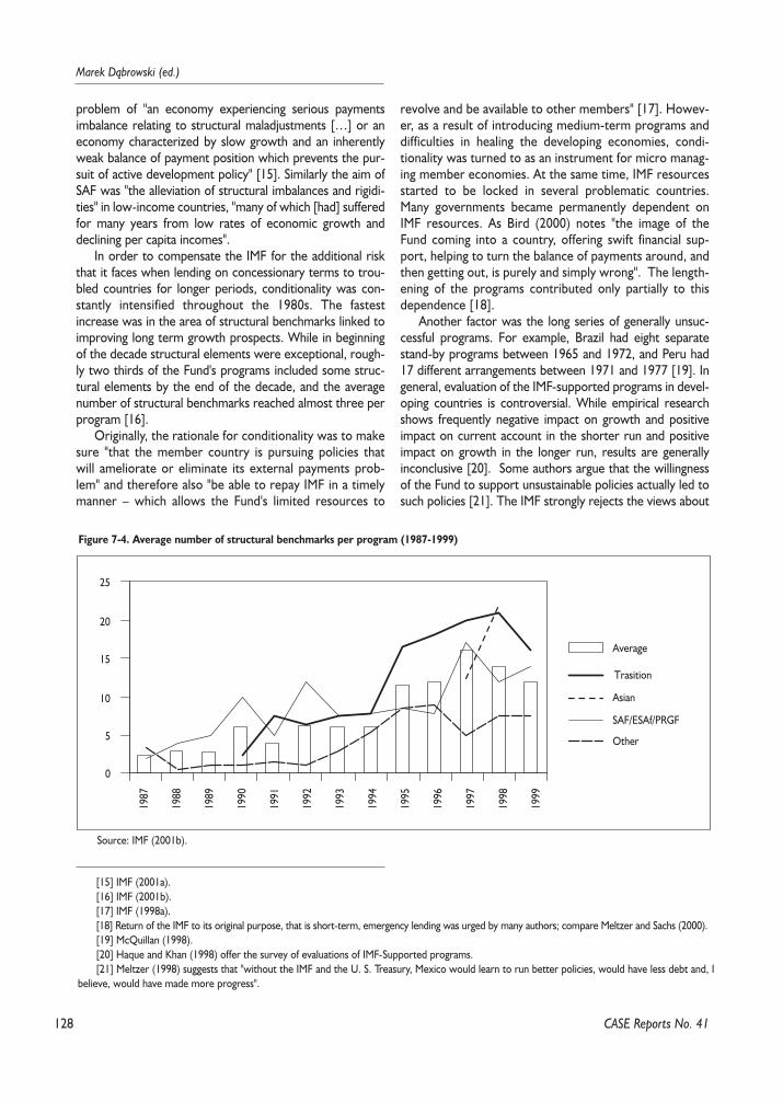
128
Marek D¹browski (ed.)
problem of "an economy experiencing serious paymentsimbalance relating to structural maladjustments […] or aneconomy characterized by slow growth and an inherentlyweak balance of payment position which prevents the pur-suit of active development policy" [15]. Similarly the aim ofSAF was "the alleviation of structural imbalances and rigidi-ties" in low-income countries, "many of which [had] sufferedfor many years from low rates of economic growth anddeclining per capita incomes".
In order to compensate the IMF for the additional riskthat it faces when lending on concessionary terms to trou-bled countries for longer periods, conditionality was con-stantly intensified throughout the 1980s. The fastestincrease was in the area of structural benchmarks linked toimproving long term growth prospects. While in beginningof the decade structural elements were exceptional, rough-ly two thirds of the Fund's programs included some struc-tural elements by the end of the decade, and the averagenumber of structural benchmarks reached almost three perprogram [16].
Originally, the rationale for conditionality was to makesure "that the member country is pursuing policies thatwill ameliorate or eliminate its external payments prob-lem" and therefore also "be able to repay IMF in a timelymanner – which allows the Fund's limited resources to
revolve and be available to other members" [17]. Howev-er, as a result of introducing medium-term programs anddifficulties in healing the developing economies, condi-tionality was turned to as an instrument for micro manag-ing member economies. At the same time, IMF resourcesstarted to be locked in several problematic countries.Many governments became permanently dependent onIMF resources. As Bird (2000) notes "the image of theFund coming into a country, offering swift financial sup-port, helping to turn the balance of payments around, andthen getting out, is purely and simply wrong". The length-ening of the programs contributed only partially to thisdependence [18].
Another factor was the long series of generally unsuc-cessful programs. For example, Brazil had eight separatestand-by programs between 1965 and 1972, and Peru had17 different arrangements between 1971 and 1977 [19]. Ingeneral, evaluation of the IMF-supported programs in devel-oping countries is controversial. While empirical researchshows frequently negative impact on growth and positiveimpact on current account in the shorter run and positiveimpact on growth in the longer run, results are generallyinconclusive [20]. Some authors argue that the willingnessof the Fund to support unsustainable policies actually led tosuch policies [21]. The IMF strongly rejects the views about
CASE Reports No. 41
Figure 7-4. Average number of structural benchmarks per program (1987-1999)
0
5
10
15
20
25
1987
1988
1989
1990
1991
1992
1993
1994
1995
1996
1997
1998
1999
Trasition
Asian
SAF/ESAf/PRGF
Other
Average
Source: IMF (2001b).
[15] IMF (2001a).[16] IMF (2001b).[17] IMF (1998a).[18] Return of the IMF to its original purpose, that is short-term, emergency lending was urged by many authors; compare Meltzer and Sachs (2000).[19] McQuillan (1998).[20] Haque and Khan (1998) offer the survey of evaluations of IMF-Supported programs.[21] Meltzer (1998) suggests that "without the IMF and the U. S. Treasury, Mexico would learn to run better policies, would have less debt and, I
believe, would have made more progress".
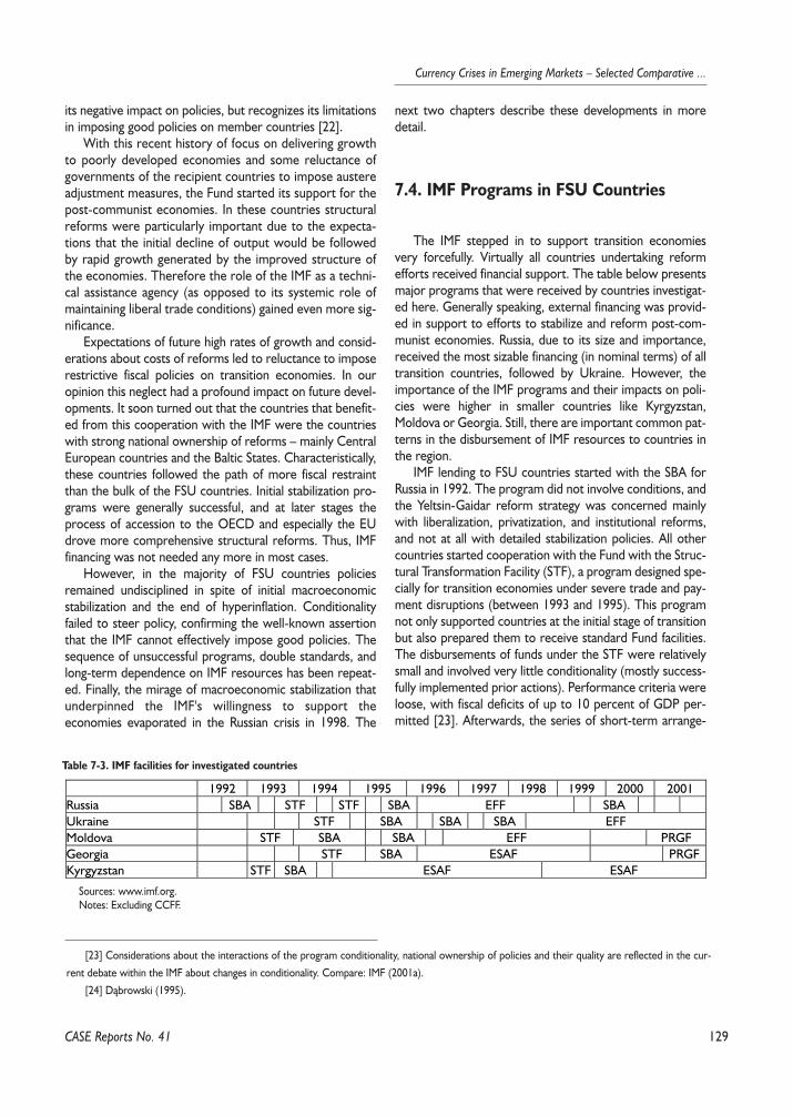
129
Currency Crises in Emerging Markets – Selected Comparative ...
its negative impact on policies, but recognizes its limitationsin imposing good policies on member countries [22].
With this recent history of focus on delivering growthto poorly developed economies and some reluctance ofgovernments of the recipient countries to impose austereadjustment measures, the Fund started its support for thepost-communist economies. In these countries structuralreforms were particularly important due to the expecta-tions that the initial decline of output would be followedby rapid growth generated by the improved structure ofthe economies. Therefore the role of the IMF as a techni-cal assistance agency (as opposed to its systemic role ofmaintaining liberal trade conditions) gained even more sig-nificance.
Expectations of future high rates of growth and consid-erations about costs of reforms led to reluctance to imposerestrictive fiscal policies on transition economies. In ouropinion this neglect had a profound impact on future devel-opments. It soon turned out that the countries that benefit-ed from this cooperation with the IMF were the countrieswith strong national ownership of reforms – mainly CentralEuropean countries and the Baltic States. Characteristically,these countries followed the path of more fiscal restraintthan the bulk of the FSU countries. Initial stabilization pro-grams were generally successful, and at later stages theprocess of accession to the OECD and especially the EUdrove more comprehensive structural reforms. Thus, IMFfinancing was not needed any more in most cases.
However, in the majority of FSU countries policiesremained undisciplined in spite of initial macroeconomicstabilization and the end of hyperinflation. Conditionalityfailed to steer policy, confirming the well-known assertionthat the IMF cannot effectively impose good policies. Thesequence of unsuccessful programs, double standards, andlong-term dependence on IMF resources has been repeat-ed. Finally, the mirage of macroeconomic stabilization thatunderpinned the IMF's willingness to support theeconomies evaporated in the Russian crisis in 1998. The
next two chapters describe these developments in moredetail.
7.4. IMF Programs in FSU Countries
The IMF stepped in to support transition economiesvery forcefully. Virtually all countries undertaking reformefforts received financial support. The table below presentsmajor programs that were received by countries investigat-ed here. Generally speaking, external financing was provid-ed in support to efforts to stabilize and reform post-com-munist economies. Russia, due to its size and importance,received the most sizable financing (in nominal terms) of alltransition countries, followed by Ukraine. However, theimportance of the IMF programs and their impacts on poli-cies were higher in smaller countries like Kyrgyzstan,Moldova or Georgia. Still, there are important common pat-terns in the disbursement of IMF resources to countries inthe region.
IMF lending to FSU countries started with the SBA forRussia in 1992. The program did not involve conditions, andthe Yeltsin-Gaidar reform strategy was concerned mainlywith liberalization, privatization, and institutional reforms,and not at all with detailed stabilization policies. All othercountries started cooperation with the Fund with the Struc-tural Transformation Facility (STF), a program designed spe-cially for transition economies under severe trade and pay-ment disruptions (between 1993 and 1995). This programnot only supported countries at the initial stage of transitionbut also prepared them to receive standard Fund facilities.The disbursements of funds under the STF were relativelysmall and involved very little conditionality (mostly success-fully implemented prior actions). Performance criteria wereloose, with fiscal deficits of up to 10 percent of GDP per-mitted [23]. Afterwards, the series of short-term arrange-
CASE Reports No. 41
[23] Considerations about the interactions of the program conditionality, national ownership of policies and their quality are reflected in the cur-rent debate within the IMF about changes in conditionality. Compare: IMF (2001a).
[24] D¹browski (1995).
Table 7-3. IMF facilities for investigated countries
1992 1993 1994 1995 1996 1997 1998 1999 2000 2001Russia SBA STF STF SBA EFF SBAUkraine STF SBA SBA SBA EFFMoldova STF SBA SBA EFF PRGFGeorgia STF SBA ESAF PRGFKyrgyzstan STF SBA ESAF ESAF
Sources: www.imf.org.Notes: Excluding CCFF.
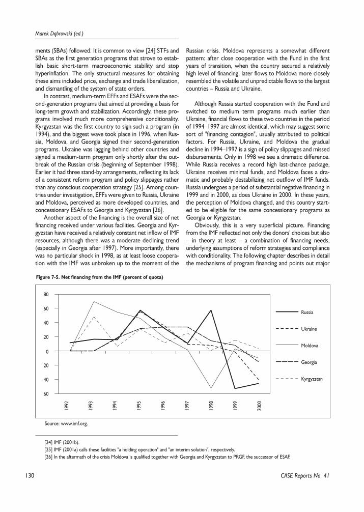
130
Marek D¹browski (ed.)
ments (SBAs) followed. It is common to view [24] STFs andSBAs as the first generation programs that strove to estab-lish basic short-term macroeconomic stability and stophyperinflation. The only structural measures for obtainingthese aims included price, exchange and trade liberalization,and dismantling of the system of state orders.
In contrast, medium-term EFFs and ESAFs were the sec-ond-generation programs that aimed at providing a basis forlong-term growth and stabilization. Accordingly, these pro-grams involved much more comprehensive conditionality.Kyrgyzstan was the first country to sign such a program (in1994), and the biggest wave took place in 1996, when Rus-sia, Moldova, and Georgia signed their second-generationprograms. Ukraine was lagging behind other countries andsigned a medium-term program only shortly after the out-break of the Russian crisis (beginning of September 1998).Earlier it had three stand-by arrangements, reflecting its lackof a consistent reform program and policy slippages ratherthan any conscious cooperation strategy [25]. Among coun-tries under investigation, EFFs were given to Russia, Ukraineand Moldova, perceived as more developed countries, andconcessionary ESAFs to Georgia and Kyrgyzstan [26].
Another aspect of the financing is the overall size of netfinancing received under various facilities. Georgia and Kyr-gyzstan have received a relatively constant net inflow of IMFresources, although there was a moderate declining trend(especially in Georgia after 1997). More importantly, therewas no particular shock in 1998, as at least loose coopera-tion with the IMF was unbroken up to the moment of the
Russian crisis. Moldova represents a somewhat differentpattern: after close cooperation with the Fund in the firstyears of transition, when the country secured a relativelyhigh level of financing, later flows to Moldova more closelyresembled the volatile and unpredictable flows to the largestcountries – Russia and Ukraine.
Although Russia started cooperation with the Fund andswitched to medium term programs much earlier thanUkraine, financial flows to these two countries in the periodof 1994–1997 are almost identical, which may suggest somesort of "financing contagion", usually attributed to politicalfactors. For Russia, Ukraine, and Moldova the gradualdecline in 1994–1997 is a sign of policy slippages and misseddisbursements. Only in 1998 we see a dramatic difference.While Russia receives a record high last-chance package,Ukraine receives minimal funds, and Moldova faces a dra-matic and probably destabilizing net outflow of IMF funds.Russia undergoes a period of substantial negative financing in1999 and in 2000, as does Ukraine in 2000. In these years,the perception of Moldova changed, and this country start-ed to be eligible for the same concessionary programs asGeorgia or Kyrgyzstan.
Obviously, this is a very superficial picture. Financingfrom the IMF reflected not only the donors' choices but also– in theory at least – a combination of financing needs,underlying assumptions of reform strategies and compliancewith conditionality. The following chapter describes in detailthe mechanisms of program financing and points out major
CASE Reports No. 41
[24] IMF (2001b).[25] IMF (2001a) calls these facilities "a holding operation" and "an interim solution", respectively.[26] In the aftermath of the crisis Moldova is qualified together with Georgia and Kyrgyzstan to PRGF, the successor of ESAF.
Figure 7-5. Net financing from the IMF (percent of quota)
60
40
20
0
20
40
60
80
Russia
Ukraine
Moldova
Georgia
Kyrgyzstan
1992
1993
1994
1995
1996
1997
1998
1999
2000
Source: www.imf.org.
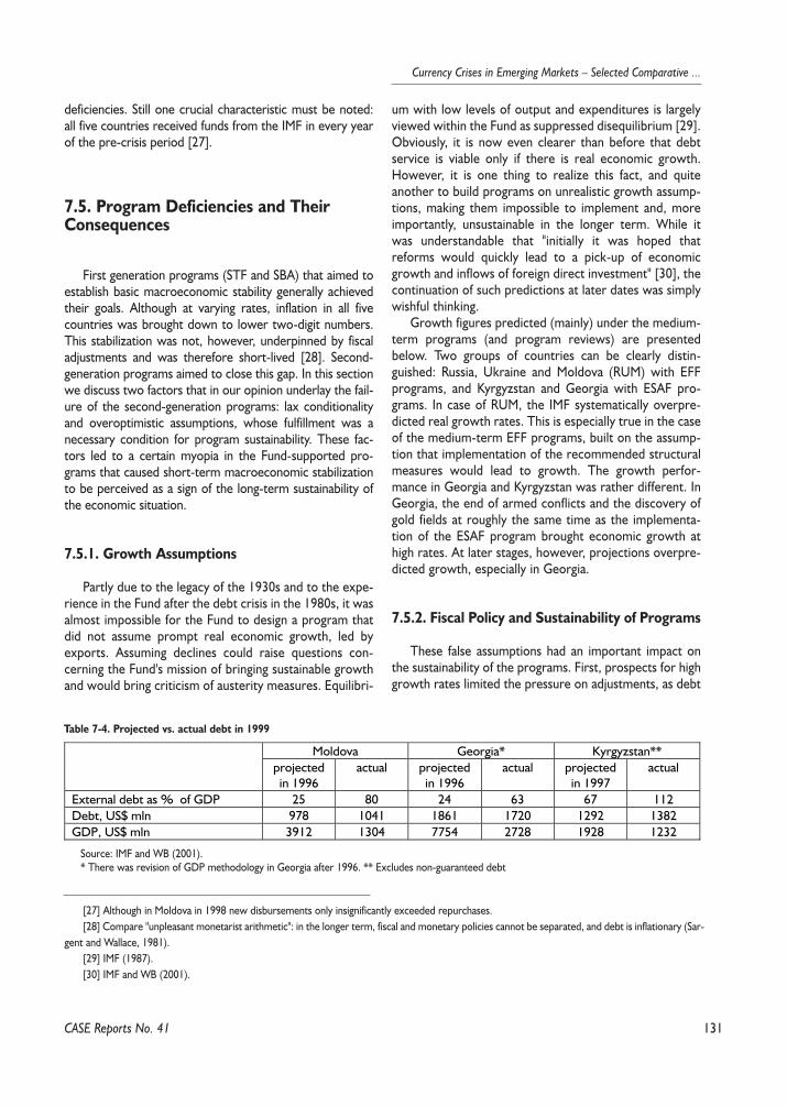
131
Currency Crises in Emerging Markets – Selected Comparative ...
deficiencies. Still one crucial characteristic must be noted:all five countries received funds from the IMF in every yearof the pre-crisis period [27].
7.5. Program Deficiencies and TheirConsequences
First generation programs (STF and SBA) that aimed toestablish basic macroeconomic stability generally achievedtheir goals. Although at varying rates, inflation in all fivecountries was brought down to lower two-digit numbers.This stabilization was not, however, underpinned by fiscaladjustments and was therefore short-lived [28]. Second-generation programs aimed to close this gap. In this sectionwe discuss two factors that in our opinion underlay the fail-ure of the second-generation programs: lax conditionalityand overoptimistic assumptions, whose fulfillment was anecessary condition for program sustainability. These fac-tors led to a certain myopia in the Fund-supported pro-grams that caused short-term macroeconomic stabilizationto be perceived as a sign of the long-term sustainability ofthe economic situation.
7.5.1. Growth Assumptions
Partly due to the legacy of the 1930s and to the expe-rience in the Fund after the debt crisis in the 1980s, it wasalmost impossible for the Fund to design a program thatdid not assume prompt real economic growth, led byexports. Assuming declines could raise questions con-cerning the Fund's mission of bringing sustainable growthand would bring criticism of austerity measures. Equilibri-
um with low levels of output and expenditures is largelyviewed within the Fund as suppressed disequilibrium [29].Obviously, it is now even clearer than before that debtservice is viable only if there is real economic growth.However, it is one thing to realize this fact, and quiteanother to build programs on unrealistic growth assump-tions, making them impossible to implement and, moreimportantly, unsustainable in the longer term. While itwas understandable that "initially it was hoped thatreforms would quickly lead to a pick-up of economicgrowth and inflows of foreign direct investment" [30], thecontinuation of such predictions at later dates was simplywishful thinking.
Growth figures predicted (mainly) under the medium-term programs (and program reviews) are presentedbelow. Two groups of countries can be clearly distin-guished: Russia, Ukraine and Moldova (RUM) with EFFprograms, and Kyrgyzstan and Georgia with ESAF pro-grams. In case of RUM, the IMF systematically overpre-dicted real growth rates. This is especially true in the caseof the medium-term EFF programs, built on the assump-tion that implementation of the recommended structuralmeasures would lead to growth. The growth perfor-mance in Georgia and Kyrgyzstan was rather different. InGeorgia, the end of armed conflicts and the discovery ofgold fields at roughly the same time as the implementa-tion of the ESAF program brought economic growth athigh rates. At later stages, however, projections overpre-dicted growth, especially in Georgia.
7.5.2. Fiscal Policy and Sustainability of Programs
These false assumptions had an important impact onthe sustainability of the programs. First, prospects for highgrowth rates limited the pressure on adjustments, as debt
CASE Reports No. 41
[27] Although in Moldova in 1998 new disbursements only insignificantly exceeded repurchases.[28] Compare "unpleasant monetarist arithmetic": in the longer term, fiscal and monetary policies cannot be separated, and debt is inflationary (Sar-
gent and Wallace, 1981).[29] IMF (1987).[30] IMF and WB (2001).
Table 7-4. Projected vs. actual debt in 1999
Moldova Georgia* Kyrgyzstan**projectedin 1996
actual projectedin 1996
actual projectedin 1997
actual
External debt as % of GDP 25 80 24 63 67 112Debt, US$ mln 978 1041 1861 1720 1292 1382GDP, US$ mln 3912 1304 7754 2728 1928 1232
Source: IMF and WB (2001).* There was revision of GDP methodology in Georgia after 1996. ** Excludes non-guaranteed debt
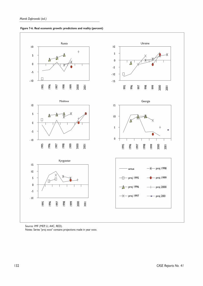
132
Marek D¹browski (ed.)
CASE Reports No. 41
Figure 7-6. Real economic growth: predictions and reality (percent)
-10
-5
0
5
10
-15
-10
-5
0
5
10
-10
-5
0
5
10
0
5
10
15
-10
-5
0
5
10
15
1995
1996
1997
1998
1999
2000
2001
actual
proj 1995
proj 1996
proj 1997
proj 1998
proj 1999
proj 2000
proj 2001
1995
1996
1997
1998
1999
2000
2001
1995
1996
1997
1998
1999
2000
2001
1995
1996
1997
1998
1999
2000
2001
1995
1996
1997
1998
1999
2000
2001
Russia Ukraine
Moldova Georgia
Kyrgyzstan
Source: IMF (MEP, LI, A4C, RED).Notes: Series "proj xxxx" contains projections made in year xxxx.
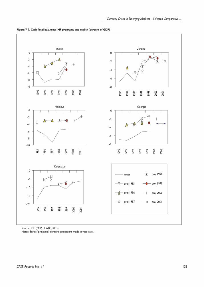
133
Currency Crises in Emerging Markets – Selected Comparative ...
CASE Reports No. 41
Figure 7-7. Cash fiscal balances: IMF programs and reality (percent of GDP)
1995
1996
1997
1998
1999
2000
2001
actual
proj 1995
proj 1996
proj 1997
proj 1998
proj 1999
proj 2000
proj 2001
1995
1996
1997
1998
1999
2000
2001
1995
1996
1997
1998
1999
2000
2001
1995
1996
1997
1998
1999
2000
2001
1995
1996
1997
1998
1999
2000
2001
Russia Ukraine
Moldova Georgia
Kyrgyzstan
-10
-8
-6
-4
-2
0
-8
-6
-4
-2
0
-10
-8
-6
-4
-2
0
-8
-6
-4
-2
0
-20
-15
-10
-5
0
Source: IMF (MEP, LI, A4C, RED). Notes: Series "proj xxxx" contains projections made in year xxxx.
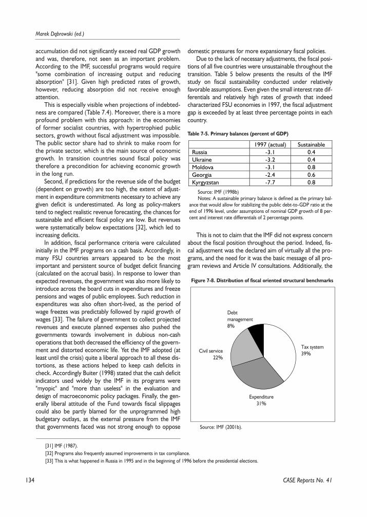
134
Marek D¹browski (ed.)
accumulation did not significantly exceed real GDP growthand was, therefore, not seen as an important problem.According to the IMF, successful programs would require"some combination of increasing output and reducingabsorption" [31]. Given high predicted rates of growth,however, reducing absorption did not receive enoughattention.
This is especially visible when projections of indebted-ness are compared (Table 7.4). Moreover, there is a moreprofound problem with this approach: in the economiesof former socialist countries, with hypertrophied publicsectors, growth without fiscal adjustment was impossible.The public sector share had to shrink to make room forthe private sector, which is the main source of economicgrowth. In transition countries sound fiscal policy wastherefore a precondition for achieving economic growthin the long run.
Second, if predictions for the revenue side of the budget(dependent on growth) are too high, the extent of adjust-ment in expenditure commitments necessary to achieve anygiven deficit is underestimated. As long as policy-makerstend to neglect realistic revenue forecasting, the chances forsustainable and efficient fiscal policy are low. But revenueswere systematically below expectations [32], which led toincreasing deficits.
In addition, fiscal performance criteria were calculatedinitially in the IMF programs on a cash basis. Accordingly, inmany FSU countries arrears appeared to be the mostimportant and persistent source of budget deficit financing(calculated on the accrual basis). In response to lower thanexpected revenues, the government was also more likely tointroduce across the board cuts in expenditures and freezepensions and wages of public employees. Such reduction inexpenditures was also often short-lived, as the period ofwage freezes was predictably followed by rapid growth ofwages [33]. The failure of government to collect projectedrevenues and execute planned expenses also pushed thegovernments towards involvement in dubious non-cashoperations that both decreased the efficiency of the govern-ment and distorted economic life. Yet the IMF adopted (atleast until the crisis) quite a liberal approach to all these dis-tortions, as these actions helped to keep cash deficits incheck. Accordingly Buiter (1998) stated that the cash deficitindicators used widely by the IMF in its programs were"myopic" and "more than useless" in the evaluation anddesign of macroeconomic policy packages. Finally, the gen-erally liberal attitude of the Fund towards fiscal slippagescould also be partly blamed for the unprogrammed highbudgetary outlays, as the external pressure from the IMFthat governments faced was not strong enough to oppose
domestic pressures for more expansionary fiscal policies. Due to the lack of necessary adjustments, the fiscal posi-
tions of all five countries were unsustainable throughout thetransition. Table 5 below presents the results of the IMFstudy on fiscal sustainability conducted under relativelyfavorable assumptions. Even given the small interest rate dif-ferentials and relatively high rates of growth that indeedcharacterized FSU economies in 1997, the fiscal adjustmentgap is exceeded by at least three percentage points in eachcountry.
This is not to claim that the IMF did not express concernabout the fiscal position throughout the period. Indeed, fis-cal adjustment was the declared aim of virtually all the pro-grams, and the need for it was the basic message of all pro-gram reviews and Article IV consultations. Additionally, the
CASE Reports No. 41
[31] IMF (1987).[32] Programs also frequently assumed improvements in tax compliance.[33] This is what happened in Russia in 1995 and in the beginning of 1996 before the presidential elections.
Table 7-5. Primary balances (percent of GDP)
1997 (actual) SustainableRussia -3.1 0.4Ukraine -3.2 0.4Moldova -3.1 0.8Georgia -2.4 0.6Kyrgyzstan -7.7 0.8
Source: IMF (1998b)Notes: A sustainable primary balance is defined as the primary bal-
ance that would allow for stabilizing the public debt-to-GDP ratio at theend of 1996 level, under assumptions of nominal GDP growth of 8 per-cent and interest rate differentials of 2 percentage points.
Figure 7-8. Distribution of fiscal oriented structural benchmarks
Tax system39%
Expenditure31%
Debt management8%
Civil service22%
Source: IMF (2001b).
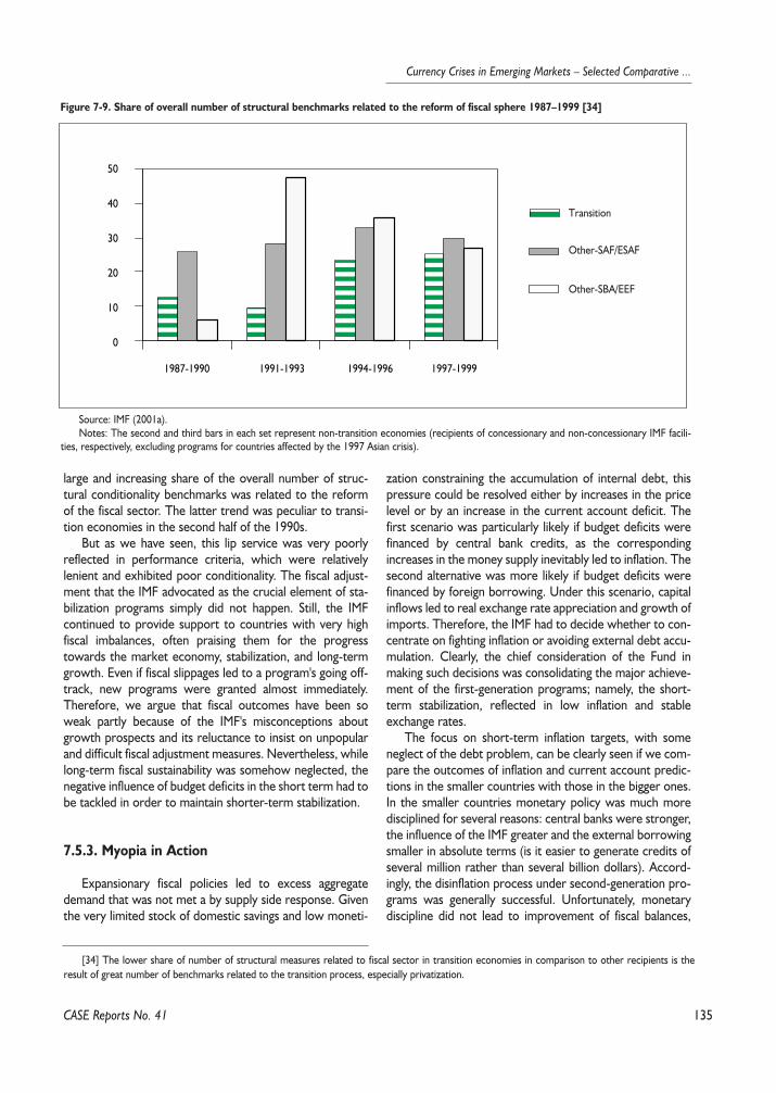
135
Currency Crises in Emerging Markets – Selected Comparative ...
large and increasing share of the overall number of struc-tural conditionality benchmarks was related to the reformof the fiscal sector. The latter trend was peculiar to transi-tion economies in the second half of the 1990s.
But as we have seen, this lip service was very poorlyreflected in performance criteria, which were relativelylenient and exhibited poor conditionality. The fiscal adjust-ment that the IMF advocated as the crucial element of sta-bilization programs simply did not happen. Still, the IMFcontinued to provide support to countries with very highfiscal imbalances, often praising them for the progresstowards the market economy, stabilization, and long-termgrowth. Even if fiscal slippages led to a program's going off-track, new programs were granted almost immediately.Therefore, we argue that fiscal outcomes have been soweak partly because of the IMF's misconceptions aboutgrowth prospects and its reluctance to insist on unpopularand difficult fiscal adjustment measures. Nevertheless, whilelong-term fiscal sustainability was somehow neglected, thenegative influence of budget deficits in the short term had tobe tackled in order to maintain shorter-term stabilization.
7.5.3. Myopia in Action
Expansionary fiscal policies led to excess aggregatedemand that was not met a by supply side response. Giventhe very limited stock of domestic savings and low moneti-
zation constraining the accumulation of internal debt, thispressure could be resolved either by increases in the pricelevel or by an increase in the current account deficit. Thefirst scenario was particularly likely if budget deficits werefinanced by central bank credits, as the correspondingincreases in the money supply inevitably led to inflation. Thesecond alternative was more likely if budget deficits werefinanced by foreign borrowing. Under this scenario, capitalinflows led to real exchange rate appreciation and growth ofimports. Therefore, the IMF had to decide whether to con-centrate on fighting inflation or avoiding external debt accu-mulation. Clearly, the chief consideration of the Fund inmaking such decisions was consolidating the major achieve-ment of the first-generation programs; namely, the short-term stabilization, reflected in low inflation and stableexchange rates.
The focus on short-term inflation targets, with someneglect of the debt problem, can be clearly seen if we com-pare the outcomes of inflation and current account predic-tions in the smaller countries with those in the bigger ones.In the smaller countries monetary policy was much moredisciplined for several reasons: central banks were stronger,the influence of the IMF greater and the external borrowingsmaller in absolute terms (is it easier to generate credits ofseveral million rather than several billion dollars). Accord-ingly, the disinflation process under second-generation pro-grams was generally successful. Unfortunately, monetarydiscipline did not lead to improvement of fiscal balances,
CASE Reports No. 41
Figure 7-9. Share of overall number of structural benchmarks related to the reform of fiscal sphere 1987–1999 [34]
50
40
30
20
10
0
1987-1990 1991-1993 1994-1996 1997-1999
Transition
Other-SAF/ESAF
Other-SBA/EEF
Source: IMF (2001a).Notes: The second and third bars in each set represent non-transition economies (recipients of concessionary and non-concessionary IMF facili-
ties, respectively, excluding programs for countries affected by the 1997 Asian crisis).
[34] The lower share of number of structural measures related to fiscal sector in transition economies in comparison to other recipients is theresult of great number of benchmarks related to the transition process, especially privatization.
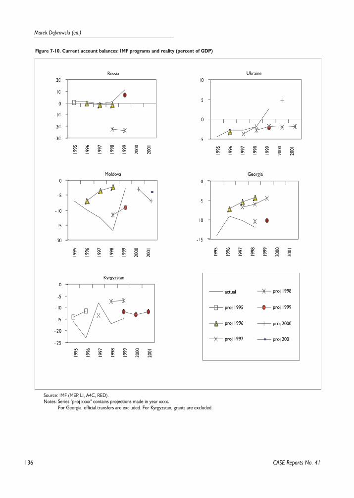
136
Marek D¹browski (ed.)
CASE Reports No. 41
Figure 7-10. Current account balances: IMF programs and reality (percent of GDP)
1995
1996
1997
1998
1999
2000
2001
actual
proj 1995
proj 1996
proj 1997
proj 1998
proj 1999
proj 2000
proj 2001
1995
1996
1997
1998
1999
2000
2001
1995
1996
1997
1998
1999
2000
2001
1995
1996
1997
1998
1999
2000
2001
1995
1996
1997
1998
1999
2000
2001
Russia Ukraine
Moldova Georgia
Kyrgyzstan
-30
-20
-10
0
10
20
-5
0
5
10
-20202
-15
-10
-5
0
-15
-10
-5
0
-25
-20
-15
-10
-5
0
Source: IMF (MEP, LI, A4C, RED).Notes: Series "proj xxxx" contains projections made in year xxxx.
For Georgia, official transfers are excluded. For Kyrgyzstan, grants are excluded.
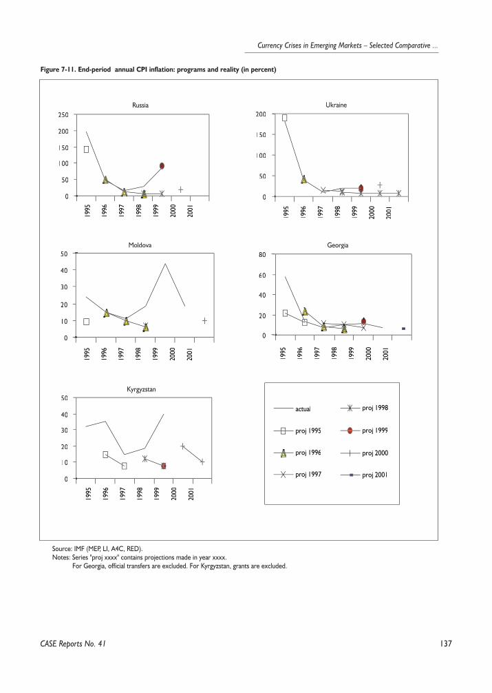
137
Currency Crises in Emerging Markets – Selected Comparative ...
CASE Reports No. 41
Figure 7-11. End-period annual CPI inflation: programs and reality (in percent)
1995
1996
1997
1998
1999
2000
2001
actual
proj 1995
proj 1996
proj 1997
proj 1998
proj 1999
proj 2000
proj 2001
1995
1996
1997
1998
1999
2000
2001
1995
1996
1997
1998
1999
2000
2001
1995
1996
1997
1998
1999
2000
2001
1995
1996
1997
1998
1999
2000
2001
Russia Ukraine
Moldova Georgia
Kyrgyzstan
0
50
100
150
200
250
0
50
100
150
200
0
20
40
60
80
0
10
20
30
40
50
0
10
20
30
40
50
Source: IMF (MEP, LI, A4C, RED).Notes: Series "proj xxxx" contains projections made in year xxxx.
For Georgia, official transfers are excluded. For Kyrgyzstan, grants are excluded.

138
Marek D¹browski (ed.)
and non-monetized budget deficits led to rapid accumula-tion of external debt. Substantial current account deficits(systematically over 10 percent of GDP in Moldova, Geor-gia, and Kyrgyzstan) were the flip side of this coin. An inter-esting example comes from Moldova, where in the firstquarter of 1998 the IMF saw a need for appreciation of theexchange rate in order to maintain low inflation [35], as thebudgetary sector was continuing to borrow abroad. Thisadvice was given irrespective of a current account deficitthat had, in the previous year, exceeded 13 percent of GDPand been covered mainly by short-term borrowing [36].This is a somewhat surprising attitude given the original roleof the IMF as the balance-of-payments watchdog.
In Russia and Ukraine, current accounts did not consti-tute a threat to macroeconomic stability, and program pro-jections were generally met. This was due partly to the rel-atively loose monetary policy: internal imbalances werereflected mainly in inflation. These countries had strongernegotiation positions vis-a-vis the IMF and weaker centralbanks. Still, one quite spectacular event occurred withrespect to the Russian current account. Just before the cri-sis, on July 20th, 1998, the IMF predicted that the currentaccount deficit would reach 9.6 billion US$ and 10.4 billionUS$ in 1998 and 1999, respectively (above 20 percent ofGDP). This shows again how unwilling the IMF was toacknowledge the unsustainability of current policies.
Our criticism is not intended to advocate more expan-sionary monetary policies, but rather we argue that the IMF
was advocating delaying the crisis (adjustment) for too long,while sending wrong signals both to governments andinvestors. Unfortunately, such policy advice was welcomedby domestic authorities, as "a finance minister faced withthis choice will almost always prefer to avoid the crisis now,at the risk of a future larger crisis, than accept the crisis nowwhen may critics are ready to claim that the crisis is avoid-able" [37].
High debt ratios are very costly because they press upreal interest rates and increase the debt service compo-nent of the deficit. In the five countries under considera-tion, debt-servicing expenditures became one of the mostimportant items on the expenditure side of the budget.The long-term costs of short-lived disinflation under loosefiscal policy appear to have been especially high for smalland highly indebted countries. Georgia and Kyrgyzstan arefollowing the path of long-term dependence on externalaid. Moldova, having disappointed initial hopes, is also setto follow this path.
When financial market participants finally refused to buynew treasury bills, governments faced three choices: adecrease in the fiscal deficit, an increase in seigniorage rev-enues, and a delay in debt repayment. In all five countrieswe observe a mix of these measures. Fiscal adjustment wascarried out with higher levels of debt, high real interestrates, limited demand for treasury securities, under manda-tory debt restructuring (e.g. Russia, Ukraine) and withweakened central bank independence.
CASE Reports No. 41
[35] IMF (1998c). The same document argues, however, that fiscal policy tightening is the major instrument for reducing macroeconomic imbal-ances and points to the increasing risk of financial and currency crisis.
[36] Real exchange rate appreciation additionally aggravated the problem due to high elasticity of import with respect to exchange rate movements.[37] Meltzer (1998).
Figure 7-12. Government external debt (percent of GDP)
160
140
120
100
80
60
40
20
0
1992
1993
1994
1995
1996
1997
1998
1999
Moldova
Georgia
Kyrgyzstan
Source: IMF and WB (2001).
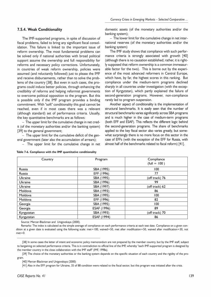
139
Currency Crises in Emerging Markets – Selected Comparative ...
7.5.4. Weak Conditionality
The IMF-supported programs, in spite of discussion offiscal problems, failed to bring any significant fiscal consol-idation. This failure is linked to the important issue ofreform ownership. The most fundamental problems canbe solved only if national authorities with broad politicalsupport assume the ownership and full responsibility forreforms and necessary policy corrections. Unfortunately,in countries of weak reform ownership, policies wereassumed (and reluctantly followed) just to please the IMFand receive disbursements, rather than to solve the prob-lems of the country [38]. But even in such cases, the pro-grams could induce better policies, through enhancing thecredibility of reforms and helping reformist governmentsto overcome political opposition to the program. But thisis possible only if the IMF program provides a bindingcommitment. With "soft" conditionality this goal cannot bereached, even if in most cases there was a relevant(although standard) set of performance criteria. Usually,the key quantitative benchmarks are as follows:
– The upper limit for the cumulative change in net cred-it (of the monetary authorities and/or the banking system)[39] to the general government;
– The upper limit for the cumulative deficit of the gen-eral government (later also the accumulation of arrears);
– The upper limit for the cumulative change in net
domestic assets (of the monetary authorities and/or thebanking system);
– The lower limit for the cumulative change in net inter-national reserves (of the monetary authorities and/or thebanking system)
The IMF study shows that compliance with such perfor-mance criteria is strongly associated with growth [40](although there is no causation established; rather, it is right-ly supposed that reform ownership is a common immeasur-able factor for the two). This is borne out by the experi-ence of the most advanced reformers in Central Europe,which have, by far, the highest scores in this ranking. Butcompliance under the medium-term programs declinedsharply in all countries under investigation (with the excep-tion of Kyrgyzstan), which partly explained the failure ofsecond-generation programs. However, non-compliancerarely led to program suspension.
Another aspect of conditionality is the implementation ofstructural benchmarks. It is easily seen that the number ofstructural benchmarks varies significantly across SBA programsand is much higher in the case of medium-term programs(both EFF and ESAF). This reflects the different logic behindthe second-generation programs. The share of benchmarksapplied to the key fiscal sector also varies greatly, but some-what surprisingly there is no more focus on this sector in thecase of EFFs (with the exception of the EFF for Russia, withalmost half of the benchmarks related to fiscal reform) [41].
CASE Reports No. 41
[38] In some cases the letter of intent and economic policy memorandum are not prepared by the member country, but by the IMF staff, subjectto bargaining on selected performance criteria. This is in contradiction to official line of the IMF, whereby "each IMF-supported program is designed bythe member country in the close collaboration with the IMF staff" (IMF, 1998a).
[39] The choice of the monetary authorities or the banking system depends on the specific situation of each country and the rigidity of the pro-gram.
[40] Mercer-Blackman and Unigovskaya (2000)[41] Also in the EFF program for Ukraine, 35 of 88 condition were related to the fiscal sector, but this program was initiated after the crisis.
Table 7-6. Compliance with the IMF quantitative conditionality
Country Program Compliance(full = 100 )
Russia SBA (1995) 100Russia EFF (1996) 77Ukraine SBA (1995) (off track) 76Ukraine SBA (1996) 99Ukraine SBA (1997) (off track) 62Moldova SBA (1993) 86Moldova SBA (1995) 100Moldova EFF (1996) 82Georgia SBA (1995) 100Georgia ESAF (1996) 89Kyrgyzstan SBA (1993) (off track) 70Kyrgyzstan ESAF (1994) 86
Source: Mercer-Blackman and Unigovskaya (2000).Remarks: The index is calculated as the simple average of compliance on each performance criteria at each test date. Compliance on a given con-
dition at a given date is evaluated using the following scale: met=100, waived=50, met after modification=50, waived after modification=30, notmet=0.
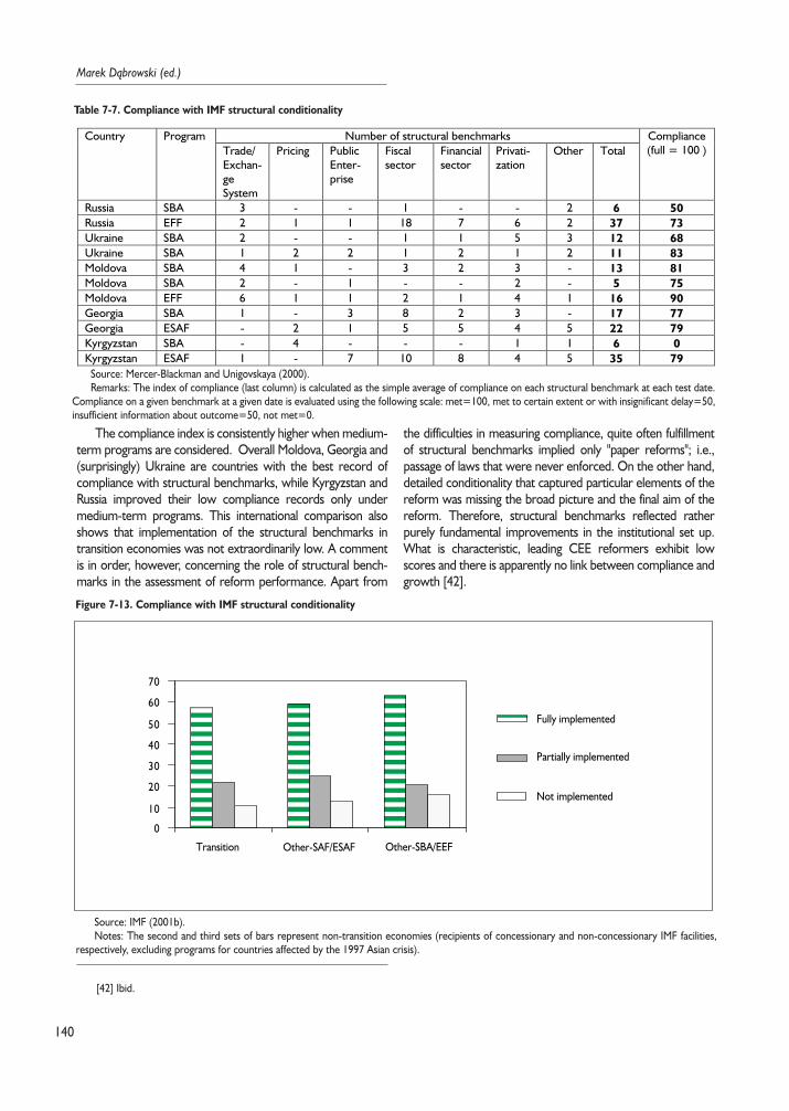
140
Marek D¹browski (ed.)
The compliance index is consistently higher when medium-term programs are considered. Overall Moldova, Georgia and(surprisingly) Ukraine are countries with the best record ofcompliance with structural benchmarks, while Kyrgyzstan andRussia improved their low compliance records only undermedium-term programs. This international comparison alsoshows that implementation of the structural benchmarks intransition economies was not extraordinarily low. A commentis in order, however, concerning the role of structural bench-marks in the assessment of reform performance. Apart from
the difficulties in measuring compliance, quite often fulfillmentof structural benchmarks implied only "paper reforms"; i.e.,passage of laws that were never enforced. On the other hand,detailed conditionality that captured particular elements of thereform was missing the broad picture and the final aim of thereform. Therefore, structural benchmarks reflected ratherpurely fundamental improvements in the institutional set up.What is characteristic, leading CEE reformers exhibit lowscores and there is apparently no link between compliance andgrowth [42].
Table 7-7. Compliance with IMF structural conditionality
Number of structural benchmarksCountry ProgramTrade/Exchan-geSystem
Pricing PublicEnter-prise
Fiscalsector
Financialsector
Privati-zation
Other TotalCompliance(full = 100 )
Russia SBA 3 - - 1 - - 2 6 50Russia EFF 2 1 1 18 7 6 2 37 73Ukraine SBA 2 - - 1 1 5 3 12 68Ukraine SBA 1 2 2 1 2 1 2 11 83Moldova SBA 4 1 - 3 2 3 - 13 81Moldova SBA 2 - 1 - - 2 - 5 75Moldova EFF 6 1 1 2 1 4 1 16 90Georgia SBA 1 - 3 8 2 3 - 17 77Georgia ESAF - 2 1 5 5 4 5 22 79Kyrgyzstan SBA - 4 - - - 1 1 6 0Kyrgyzstan ESAF 1 - 7 10 8 4 5 35 79
Source: Mercer-Blackman and Unigovskaya (2000).Remarks: The index of compliance (last column) is calculated as the simple average of compliance on each structural benchmark at each test date.
Compliance on a given benchmark at a given date is evaluated using the following scale: met=100, met to certain extent or with insignificant delay=50,insufficient information about outcome=50, not met=0.
Figure 7-13. Compliance with IMF structural conditionality
0
10
20
30
40
50
60
70
Fully implemented
Partially implemented
Not implemented
Transition Other-SAF/ESAF Other-SBA/EEF
Source: IMF (2001b).Notes: The second and third sets of bars represent non-transition economies (recipients of concessionary and non-concessionary IMF facilities,
respectively, excluding programs for countries affected by the 1997 Asian crisis).
[42] Ibid.
141
Currency Crises in Emerging Markets – Selected Comparative ...
The official IMF evaluation of first- and second-generationprograms in RUMGK indicates rather high compliance withIMF conditionality. In our opinion this is highly questionable.Russia, the FSU country most generously financed by the IMF,
provides the most striking evidence of non-compliance. Weanalyze this case in detail below. However, very similar patternswere clearly visible in the other four countries [43].
CASE Reports No. 41
Box 1: IMF Conditionality: The case of Russia
The IMF decided not to put rigorous conditions on the SBA in 1992, and the Yeltsin-Gaidar reform program dealtmainly with liberalization, privatization, and institutional reforms, and not at all with detailed stabilization policies. The onedistinctive feature of this stabilization plan was that neither the wage nor the exchange rate would serve as a nominalanchor. The inflation objective was below 5 percent per month, which was not very ambitious. The political weakness ofthe Yeltsin-Gaidar government became apparent with the nomination of Victor Gerashchenko, who represented inter-ests of lobbies (industrialists, regions, FSU countries, etc.) demanding credits from the authorities, as Chairman of theCentral Bank of Russia. Monetization of an enlarged government deficit representing almost 20 percent of GDP and gen-erous credit lines to the FSU countries led to CPI inflation of over 20 percent monthly in the fourth quarter of 1992. Obvi-ously, all the IMF targets were exceeded at the very beginning of the program in September-October 1992. In the over-all appraisal of the achievements of Yeltsin-Gaidar program, the defeats outnumbered the gains. The macroeconomic pol-icy lacked monetary and fiscal tightening. The policy of the CBR was aimed at supporting production and propping upfinancially inefficient state enterprises and cooperative farms. Foreign trade was only partly liberalized. Incomplete dereg-ulation of prices (combined with the slow pace of demonopolization of the economy) caused shortages, and pressure formassive state interventions (softening of monetary and fiscal policies) grew. The Yeltsin-Gaidar government decided notto start privatization of agriculture. Finally, both the IMF and the Russian authorities followed an inconsistent policy relat-ed to abandoning the ruble zone with other ex-Soviet republics, which led to huge transfers of the Russian GDP and fur-ther boosted inflation. In December 1992 Yegor Gaidar was replaced by Victor Chernomyrdin, a moderate representa-tive of the "red directors" lobby preferred by the majority of parliamentarians.
The first Article IV consultation was concluded on April 21, 1993 [44]. On June 30, 1993, the Executive Boardapproved an economic program to be supported by a two-tranche purchase under the Systemic Transformation Facility(STF). Russia purchased the first tranche of SDR 1,078.3 million (equivalent to 25 percent of quota) from the IMF on July6, 1993. The STF, as a brand-new IMF facility, made it possible to credit the new Russian government irrespective of thefailure of the previous program. Also, there were many new features in the program. Firstly, the STF specified that thepurchase from the IMF would not have to be added to the stock of Russia's official international reserves but would beavailable to provide additional credit to the economy (and to the budget). This represented a major departure from theIMF's primary goal of providing financial assistance to countries experiencing temporary balance of payments problems.In doing so, the IMF entered terrain usually reserved for the World Bank and its agencies financing government projects(or, more precisely, budgetary expenditures). The conditions of the STF program remained broadly the same as those ofthe SBA, but this time included explicit targets rather than soft projections.
The program got off to a good start, but as early as the third and the fourth quarters of 1993, targets were exceed-ed by wide margins. The reason was that tight monetary policy was not accompanied by fiscal adjustment, as PresidentBoris Yeltsin vetoed the 1993 budget (with a deficit of 20 percent of GDP) and then dissolved the Supreme Soviet. In thelast months of 1993, Minister of Finance Boris Fedorov made an attempt to limit expenditures and refused to pay. Theresult of sequestration was a buildup in government arrears, some of which would have to be repaid. Therefore, mostmonetary and fiscal conditions were not fulfilled. Also, the fulfillment of the monetary conditions was spurious as the offi-cial increase in the CBR interest rate brought preferential central banks credits below this rate. Accordingly, the next IMFcondition, concerning liberalization of the exchange rate, ended up in CBR interventions to maintain the exchange rateof around 1000 rubles per U.S. dollar. Real appreciation of the ruble led to an increase in imports, dwindling reserves,and finally depreciation of the ruble by 20 percent in September-October 1993. The second tranche of STF was to bedisbursed in September 1993, after a review of the program; however, the failures of 1992 were repeated, and all con-ditions were broken within a quarter after the signing of the agreement.
[43] These cases are not included in this article in order to avoid repetition. [44] According to Article IV, Section 3 of the IMF Articles of Agreement, the IMF has the mandate to oversee the compliance of each member with
its obligations, and each member should provide the IMF with necessary information.

142
Marek D¹browski (ed.)
CASE Reports No. 41
On April 20, 1994, the IMF Executive Board approved the next program of the new Russian government [45] sup-ported by a second tranche of SDR 1,078.3 million under the STF. The major goal of the program was to safeguard thefragile achievements in the Russian reforms, especially in the areas of price and exchange rate liberalization, and fosterstructural reforms, including privatization, foreign trade liberalization , increased competition, and transparency. Gradu-alism was officially the key operating concept both for Prime Minister Victor Chernomyrdin and the IMF. Again, condi-tions of the second STF program were similar to those of the first STF.
The second STF combined the macroeconomic conditionality of the first STF with structural reforms, especially massprivatization, managed by Anatoly Chubais, who was in charge of the State Privatization Committee. In the second quar-ter of 1994 program implementation was on target. The monthly inflation rate fell to 6 percent in June 1994 and to 4.5percent in August 1994. The government managed to keep its borrowing from the central bank within the program tar-gets, but mainly through aggressive sequestration of expenditures as budget revenues collapsed. In the third quarter, how-ever, credits from the central bank surged as revenues fell in relation to GDP and subsidies to agricultural sector, the North-ern Territories, and other customary recipients of budget financing rose sharply. The government's ability to use seques-tration diminished and the Parliament rejected most of the revenue measures specified in the second STF. In mid-1994, theauthorities ran down official reserves in an attempt to offset the impact of the surge in net credit to the government onthe monetary base and inflation. After international reserves dropped by almost US$4 billion in the third quarter of 1994,foreign exchange market participants started to speculate against the ruble. Market participants were fully aware of theinconsistencies in the expansionary fiscal policy and quasi-tightening of monetary policy, which limited credits to banks butexpanded financing of the deficit. On October 11, 1994, the ruble tumbled in the Moscow interbank market by over 20percent against the U.S. dollar. "Black Tuesday" became the first currency crisis in post-communist Russia. In the fourthquarter of 1994, the central bank limited credit expansion to banks and the government, and the Ministry of Financerestricted expenditures but also started issuing government securities well below the market rate [46]. The credit crunchled to a rise in interest rates, but inflation continued to increase reaching a monthly rate of 16 percent in December 1994- twice the STF projection. Fiscal targets were exceeded by wide margins, the stock of international reserves droppedbelow the target, the exchange rate depreciated by 45 percent during the second half of 1994, and the majority of liber-alization measures was not implemented. The second STF failed as completely as its predecessor.
The rise in inflation, the accumulation of government arrears, and the exchange rate crisis on October 11, 1994, ledto the next reshuffling of the Russian Cabinet. Finance Minister Sergei Dubinin and CBR governor Victor Gerashchenkowere fired. Anatoly Chubais was appointed First Deputy Prime Minister in charge of economic policy, Yevgeny Yasinbecame Minister of the Economy, and Tatyana Paramonova became Acting Chairperson of the CBR. Negotiations withthe IMF resumed, this time concerning a program that would be supported by a stand-by credit of up to SDR 4,313 mil-lion (100 percent of quota). As in previous years, a major tightening of monetary and fiscal policies took place at the begin-ning of 1995. In January, the stock of credit to the government was frozen, the CBR increased reserve requirements, and– as international reserves kept declining – the monetary base shrank by 9 percent. Inflation slowed to 10–11 percent inFebruary-March. On March 10, 1995, in a letter to IMF Managing Director Michel Camdessus, President Boris Yeltsinexpressed his support for the new arrangement. On April 11, 1995, the IMF Executive Board approved the stand-byarrangement supported by a credit of SDR 4,313.1 million for a period of 12 months. Additionally, the IMF waived Arti-cle V, Section 3(b)(iii), and increased the limit of lending to 200 percent of the Russia's quota. According to official state-ments, the SBA was aimed at decisive progress in stabilization and structural reform during 1995 and envisaged the samemeasures as in the previous programs, both from macroeconomic and structural perspective.
In the course of the stand-by program quantitative targets were all met month by month with comfortable margins.The most vulnerable situation remained in the fiscal sector, because of substantial revenue shortfalls that persistedthroughout 1995. Measures to improve revenues were implemented only partially or with a lag. Major revenue cate-gories barely exceeded the program's projections in nominal terms in spite of substantially increased inflation, and for1995 the ratio of revenue to GDP turned out to be nearly 3 percentage points below the programmed level. Under thesecircumstances, in order to meet the deficit target the authorities contained spending (in relation to GDP), keeping itbelow programmed levels. On the monetary side, while credit targets were met, large capital inflows put pressure onthe ruble, leading to nominal and real appreciation and/or growth of the monetary base (given limited capacity for ster-ilization). Growing confidence in the ruble and the increase in reserves allowed for introduction of an exchange rate cor-
[45] Victor Chernomyrdin remained Prime Minister and Sergei Dubinin was nominated as Minister of Finance.[46] Issuance of new kinds of government bonds, including medium-term ones, was planned in the second STF program with a goal to establish a
market for government securities and increase the portion of non-inflationary financing of the budget deficit.
143
Currency Crises in Emerging Markets – Selected Comparative ...
ridor on July 5, 1995 (4,300 - 4,900 ruble per U.S. dollar). However, in the second half of October, pre-election pressurebecame evident as fiscal policy started to drift away from targets. The previously accumulated margins (with respect tothe cumulative ceilings for the credit aggregates, fiscal deficit, and international reserves) allowed the targets for Octoberand November to be met. In December (especially in the last ten days of the month), the authorities probably used "win-dow dressing" to achieve the targets. Therefore, the tendency of policies to drift in the last quarter continued in 1995,and as with the previous programs, it had a negative impact on inflation (3.5 percent in December 1995, instead of 1 per-cent).
Structural reforms, especially bank restructuring, were considered relatively sluggish. This became evident when aninterbank liquidity crisis emerged toward the end of August 1995. The pace and scale of privatization fell short of expec-tations, and transparency of the whole process due to the introduction of the loans-for-shares scheme became doubtful.Finally, little progress was achieved in the area of land reform.
Summing up, in 1995 the Russian authorities apparently decided to fulfill macroeconomic targets but abandon struc-tural reforms that conflicted with the interests of various lobbies and were therefore politically difficult. The relative suc-cess of the 1995 stand-by (in comparison with the performance of the previous arrangements) allowed the Russianauthorities to request IMF support for the medium-term program of macroeconomic stabilization and structural reform.
In a letter dated March 6, 1996, the Russian government requested a three-year arrangement under the EFF in theamount of SDR 6,901 million, or 160 percent of the quota. The ongoing stand-by program would then be cancelled as ofthe date of approval of the extended arrangement. This trade off yielded positive results: almost immediately, on March26, 1996, the IMF Board approved the program (and again waived Article V).
The proposed strategy for 1996–1998 aimed at establishing a foundation for sustainable growth by lowering inflationto a single-digit annual rate, implementing key structural reforms, and achieving medium-term viability of the balance ofpayments. The 1996 program was based on quite optimistic forecasts, such as a high annual rate of GDP growth (6 per-cent starting in 1997), 1 percent inflation monthly beginning at the end of 1996, recovery of money demand, repatriationof flight capital, increase in foreign direct investments, and a comprehensive restructuring of debt obligations (US$7 bil-lion). The debt service burden was especially large for the federal budget, as the accumulation of maturities and arrearsduring the following years was already foreseen in 1996. However, the critical element of the medium-term strategy wasa further reduction in the overall fiscal deficit of the general government from around 6 percent of GDP in 1995 to 4 per-cent of GDP in 1996 and 2 percent of GDP in 1998. Local governments and off-budget funds were to balance their bud-gets or finance deficits from non-inflationary sources (without credits from the CBR). A net increase in revenues of closeto 5 percentage points of GDP was planned for the medium term (via an increase in tax rates and broadening of the taxbase through elimination of tax exemptions and preferential treatment, especially for fuel producers). The monetaryframework targeted the same parameters as previous programs, limiting the pace of credit expansion and monetizationof the budget deficit. The programmed domestic assets expansion would not result in growth of the monetary basebecause it was exactly offset by a decline in the monetary authorities' net international reserves. The same was true ofthe 1995 program – the sale or use of government reserves was included as part of the monetary authorities' net creditto the federal and enlarged governments. Therefore, the IMF's intention was clearly non-inflationary deficit financing.
The period of 1996–1998 reflected elusive macroeconomic stabilization. Since 1995, Russia had not been able toachieve its main fiscal policy objectives, which were a reduction in the unsustainably high deficit, a reversal of the declinein budget revenues, and a reduction of expenditures. The general government primary deficit rose from 2.6 percent ofGDP in 1995 to 3.1 percent of GDP in 1997, and the overall deficit increased from 6.1 percent to 7.7 percent of GDP inthe same period. At the same time, general government revenues only increased from 33.5 percent of GDP in 1995 to35.5 percent of GDP in 1997, whereas expenditures increased from 39.6 percent to 43.2 percent of GDP in the sameperiod. This reflected a number of fundamental factors, but perhaps the most important among them was a continuedrecourse to non-monetary fiscal operations and tax offset schemes on the revenue side and expansion of interest pay-ments on the debt on the expenditure side [47].
In mid-1998, the accumulation of macro- and microeconomic problems coincided with the cumulating maturity ofdebt payments due in the third quarter of 1998, amounting to one third of budget revenues, and with a current accountdeficit resulting from a decline in world fuel prices. Moreover, the Asian crisis in 1997–1998 had increased financial mar-ket volatility and investor pessimism about the performance of the Russian economy.
Some adjustment measures implemented at the beginning of 1998 by the government of Prime Minister SergeiKiriyenko, especially sequestration of expenditures and proposed changes in tax law, were not effective (the Parliament's
CASE Reports No. 41
[47] See Antczak (2000) for an analysis of the Russian crisis in 1998.

144
Marek D¹browski (ed.)
willingness to support the government's plans was very limited). Capital flows remained volatile and market confidencewas not restored. The Russian authorities proposed to implement radical measures and expected support from the IMF.On July 16, 1998, a Memorandum of the Government of the Russian Federation and the Central Bank of the Russian Fed-eration on Economic and Financial Stabilization Policies was signed with the IMF. The government program was basicallyidentical to those supported by the IMF but not realized throughout the previous five years. It aimed at radically tighten-ing the federal budget and lengthening debt maturity, and the authorities expected "substantial foreign financing" for theprogram. The proposed package of measures for 1998 was partially based on the ongoing EFF arrangement. However,the Duma rejected the proposed changes in tax policy (broadening the base of the Personal Income Tax and transferringa higher share of PIT revenues to the federal budget, increasing the land tax, and balancing the budget of the PensionFund). The Russian government was to provide a supplementary memorandum to the IMF on July 20. On July 31, the IMFtried to avert crisis by disbursing a SDR 3.4 billion tranche, irrespective of the lack of a formal agreement. However, this
CASE Reports No. 41
Figure 7-14. Russian Federation, compliance with the IMF quantitative monetary, fiscal, and exchange rate targets in 1993-1999 (%)
- 500
0
500
1000
1500
2000
2500
3000
3500
4000
-2000
0
2000
4000
6000
8000
10000
12000
14000
16000
milli
ons o
f USD
milli
ons o
f USD
Net flows (LHS) Net cumulative flow (RHS)
92M
01
93M
01
94M
01
95M
01
96M
01
97M
01
98M
01
99M
01
00M
01
00M
03
Source: IMF (A4C, IFS, RED, SP) Note: Exceeding of targets should be viewed as noncompliance with conditionality. Targets are equally weighted. The inflation target was
officially stated as an objective or projection, and after 1995 was not included in the IMF conditionality.
Figure 7-15. IMF net disbursements to Russia in 1992-2001 (millions of US$)
93M
06
93M
12
94M
06
94M
12
95M
09
96M
03
96M
09
97M
03
97M
09
98M
03
98M
09
99M
03
99M
09
Monetary (LHS) Fiscal (LHS) Forex reserves (RHS) Inflation (RHS)
800
600
400
200
0
-200
-400
-600
-800
%
100
75
50
25
0
-25
-50
-75
-100
%
Source: www.imf.org.

145
Currency Crises in Emerging Markets – Selected Comparative ...
in fact only hastened the inevitable deep correction of the exchange rate made necessary by accumulated macroeconomicimbalances.
With the crisis of August 1998, Russia exceeded all quantitative targets established in the EFF program. IMF dis-bursements to Russia came to a halt. The latest program, an SBA for SDR 3.3 billion (55.5 percent of quota) for a periodof 17 months, was signed on July 28, 1999. Through the end of 2000, Russia has made only one purchase. Quantitativeperformance criteria for the end of July, the end of September, and the end of December 1999 were reached (many withlarge margins). However, there were many shortfalls relative to structural benchmarks for the third and fourth quartersof 1999.
CASE Reports No. 41
The example of Russia (to which we could easily addsimilar cases from the other four countries) clearly showsthat from the very beginning of the transformation the IMFwas not insistent enough on its conditionality, especially inthe area of fiscal adjustment. It also shows that the condi-tionality was effectively much weaker than is suggested bythe relatively high scores on compliance presented by IMFsources. This inconsistency stems from issues of trans-parency in the performance criteria. The attempts to cir-cumvent imprecision were also one of the reasons for theproliferation of arrears, sequestration, explicit and implicitguarantees, and quasi-fiscal operations. It is important thatthe majority of "more than useless" indicators were createdin the crucial sector of public finance. While the promotionof public awareness and responsibility should be one of keyfunctions of the Fund [48], it has long given a rather ideal-ized picture of the FSU countries. The public could not gen-erally access surveillance data or memoranda on policies orcriteria breaching. Instead, as Boris Fedorov put it, "the IMFwas pretending that it was seeing a lot reforms. Russia waspretending to conduct reforms" [49]. Similarly, The Econo-mist (1996) quotes an anonymous Russian minister's com-ments on the March 1996 negotiations to the effect that"bookkeeping tricks were pulled on both sides".
A further factor in the weakening of conditionality wasthe changing weight given to performance criteria and pro-gram reviews. Performance criteria (and prior actions)should generally be very precisely defined and provide aready test for the compliance of policies with the program.Non-implementation can still be accepted through theissuance of a waiver; however, conditionality based on per-formance criteria is generally less lax and less likely to beaffected by political considerations. On the other hand, pro-gram reviews that mix ex-post evaluation with expectationstowards future actions provide much more room for dis-cretion. Coupled with the increasing number of waivers andmodification in the program criteria, this undermined the"binding commitment" role of conditionality. The final, and
probably most important, factor behind lax conditionality isthe ease with which the Fund continued to work with coun-tries with very bad track records. Again, the case study ofRussia shows this very clearly, but a similar pattern can beobserved in most of the countries under investigation here:new programs were continually covering up the fundamen-tal weakness of the FSU economies.
To sum up, the conditionality exhibited excessive lenien-cy, allowing recipient countries to avoid fiscal and otherkinds of necessary adjustment. While flexibility is important,as it allows for corrective measures in cases of externalshocks, it has been clearly abused in the case of the FSU.Again, the prior experience of the IMF appears to be atfault. Instead of promoting good policies in a decisive man-ner, the Fund was showing that it "pays due regard to thedomestic social and political objectives" [50] - even if theseobjectives were detrimental to long-term growth and stabi-lization.
7.5.5. Soft Financing
Throughout this paper we have argued that the IMF wasnot insistent enough on fiscal adjustment. We now wish totake this argument further and show that the IMF programswere actually detrimental to true fiscal adjustment. As theIMF was consistently softening governments' "hard budgetconstraints" by providing non-monetary sources of deficitfinancing, the political support for fiscal tightening was evenmore difficult to generate than would have been the case inthe absence of IMF programs.
The support of the IMF for the development of non-monetary deficit financing in RUMGK was twofold. First, theIMF was willing to indirectly finance FSU governments. TheSTF in 1993 specified that the purchase from the IMF wouldnot have to be added to the stock of Russia's official inter-national reserves but would be available to provide addi-tional credit to the economy (and to the budget). The same
[48] Compare, for example, Brown (1998).[49] Cited in McQuillan (1998).[50] IMF (2001a). Compare also Camdessus (1994): "(…) policies may indeed need to be adjusted pragmatically in light of circumstances and devel-
opments. One example has been fiscal policy. (…) In many cases, after careful assessments, the Fund has agreed in these circumstances to the tem-porary relaxation of fiscal deficit targets in programs it has supported, while of course continuing to focus on the requirements of lowering inflationand achieving medium-term fiscal sustainability". Developments proved, however, that it is extremely difficult to achieve sustainability when adjust-ments are repeatedly delayed and "temporary relaxations" persist.

146
Marek D¹browski (ed.)
was the case of the 1995 program: the sale or use of gov-ernment holdings of reserves was included as part of themonetary authorities' net credit to the federal and enlargedgovernments. In so doing, the IMF was attempting to financethe budget deficit in a non-inflationary manner. Indeed, inour five countries, all of whose central banks were directlyfinancing the budgets, the IMF funding was transferred tothe budget and consumed. Ukraine serves as a good exam-ple. The Ukrainian EFF program included a target for cen-tral bank gross purchases of treasury bills from the primarymarket. Agreements with the IMF also allowed for negotia-tions with debtors on rescheduling of payments. Suchreschedulings were to constitute a source of balance of pay-ment financing referred to as "exceptional financing". Russia,as the legal successor to the debt (as well as the assets) ofthe USSR and net creditor to the rest of the FSU countries,received the largest rescheduling of debt payments. Theexistence of the ruble area until July 1993, inter-republican
trade and financial links, and the similarity of transformationproblems led to the adoption of a common approach to allFSU countries by the Western governments and interna-tional financial institutions. In practice, informal reschedulingof the Russian debt payments was often conditioned on theRussian government's rescheduling of debt payments it wasowed by Ukraine, Moldova, Georgia, or Kyrgyzstan. Thismultilateral credit approach was used in relations amongstmost FSU countries. Therefore, the IMF disbursements can– together with exceptional financing (i.e., debt relief andarrears) – be treated as a form of financing of the twindeficits (balance of payments and budget deficits).
The unjustified "seal of good housekeeping" further soft-ened budget constraints, as the economic policy memoran-da with the IMF opened the door to cooperation with othermultilateral and bilateral donors. IMF programs constituteda stamp of approval for government policies, tending tobring improvements in the countries' ratings and new capi-
CASE Reports No. 41
Figure 7-16. Balance of payment gap and financing (1994-1999)
Russia19
94Q
1
1995
Q1
1996
Q1
1997
Q1
1998
Q1
1999
Q1
15001000
5000
-500-1000-1500-2000
60
40
20
0
-20
-40
-60
1994
Q1
1995
Q1
1996
Q1
1997
Q1
1998
Q1
1999
Q1
1994
Q1
1995
Q1
1996
Q1
1997
Q1
1998
Q1
1999
Q1
1994
Q1
1995
Q1
1996
Q1
1997
Q1
1998
Q1
1999
Q1
Ukraine Kyrgyzstan
Mo³dova
BOP gap IMF & exceptional financing * IMF financing
1500
1000
500
0
-500
-1000
-1500
100
50
0
-50
-100
-150
Source: IMF (IFS)Note: The balance of payments gap is defined here as the sum of the current account, capital account, financial account, and errors and omissions.
IMF and exceptional financing are financing items in the balance of payments. The residual from these two is the change in net international reservesof the monetary authorities.
147
Currency Crises in Emerging Markets – Selected Comparative ...
tal inflows. This catalytic role is explicitly recognized as oneof the main functions of the IMF in support of adjustment.However, when the IMF underwrites unsustainable policies,the effect is disastrous for the borrowing country: externaldebt accumulates and incentives for adjustments are dimin-ished.
For smaller countries this foreign financing led to a debttrap. Wrong signals sent to private creditors and govern-ments had a highly detrimental impact on the economic sit-uation of these countries. Policies based on increasing debt-to-GDP ratios were unsustainable, but could be maintainedas long as financial markets did not fully realize this. Aninteresting example of such an attempt to change marketsentiment was the arrangement negotiated for Russia in1998, which aimed to use external financing to prolong thefragile stabilization [51]. Later on, however, the IMF admit-ted that crisis was inevitable unless the "steadier process atwork" were fundamentally reversed [52].
Worse, a general sense of implicit guarantees ("too bigto fail"), especially in case of Russia, was built up over thecourse of years. While the role of IMF in the modern worldshould be the prevention of crisis through the surveillanceof national policies, transparent information and reductionof moral hazard, the practice was exactly opposite. Meltzer(1999) concludes: "Moral hazard lending to Russia, encour-aged by the bail out of foreign lenders to Mexico, permittedRussia and other countries to finance large unbalanced bud-gets by borrowing externally. The result is a much largerfinancial problem for international lenders and for theeconomies of other countries". In consequence, the IMF'sopening of access to external savings delayed the change indirection of capital flows and therefore induced reluctanceto apply remedies. Without the IMF, Russia and other coun-tries in the region might have had better policies.
7.6. Conclusions: Political and Institutional Considerations
How could the IMF have made such mistakes? Theanswer to this question is basically beyond scope of thispaper. We will simply note that it is most likely of a politicalnature. As Meltzer (1999) [53] explains: "The G-7 govern-ments either were unwilling or believed themselves unable
to obtain funding for the transformation from their parlia-ments. The IMF agreed to accept responsibility. In doing so,it reached far beyond its competence". The influence of pol-itics over economics, and especially on the quality of condi-tionality, can be summarized in the popular adage that "sav-ing Russia from communism matters more than the nicetiesof monthly bookkeeping" [54]. Another group of factorsthat could contribute to this problem is related to the sys-tem of incentives facing the IMF bureaucracy [55]. The IMFas an institution has a stake in the "success" of the program.It is, therefore, difficult for its officials to declare the pro-gram a failure, even if it cannot impose its real implementa-tion. Finally, the IMF wants to stay in the country, as it con-siders some influence on policy to be better than no influ-ence at all. This is, however, not the case if it leads the Fundto underwrite bad policies.
CASE Reports No. 41
[51] Stanley Fischer (1998) stated at the beginning of 1998 that "the Russian economy has broadly achieved stabilization and the future should bringmuch more peaceful days".
[52] IMF (RED) on Russia, issued in September 1999.[53] Compare also Dabrowski (1995). Several authors argue that a politically independent IMF would be more effective at promoting international
financial stability; compare De Gregorio et al. (2000).[54] The Economist (1996)[55] Vauber (1994)

148
Marek D¹browski (ed.)
References
Antczak R. (2000). "The Russian Crisis of 1998, CASE,mimeo.
Bandow D., I. Vasquez, eds. (1994). "PerpetuatingPoverty". The World Bank, the IMF and the DevelopingWorld.
Bird G. (1995). "IMF Lending to Developing Countries".Issues and Evidence, London.
Brown G (1998). "Statement: Steering a Course for Sta-bility". Summary Proceedings.
Buiter W.H. (1997). "Aspects of Fiscal Performance insome Transitions Economies Under Fund-Supported Pro-grams". IMF Working Paper No. WP/97/31.
Camdessus M. (1994). "Supporting Transition in Centraland Eastern Europe: An Assessment and Lessons from theIMF's Five Years' Experience". IMF Speeches No.95/2.
Dabrowski M. (1995). "Western Aid Conditionality andthe Post-Communist Transition". CASE, Studies and Analy-ses No. 37.
Dabrowski M. ed. (1999). "Disinflation, Monetary Policyand Fiscal Constraints. Experience of the Economies inTransition". CASE Reports No. 16.
Dabrowski M. ed., (1999b). "Ukraine: From Fragile Sta-bilization to Financial Crisis". CASE, Studies and Analyses,No. 158.
De Gregorio J., B. Eichengreen, I. Takotoshi, C. Wyplosz(2000). "An Independent and Accountable IMF". GenevaReports on the World Economy, No. 1.
Fischer S. (1998). "The Russian Economy at the Start of1998". IMF, Speeches, January 9.
Fischer S., R. Sahay (2000). "The Transition EconomiesAfter Ten Years". IMF Working Paper No. WP/00/30.
Friedman M. (1998). "Markets to the Rescue". WallStreet Journal, 13 October.
Gomulka S. (1995). "The IMF-supported programs ofPoland and Russia, 1990–1994: principles, errors andresults". CASE, Studies and Analyses No. 36.
Gomulka S. (2000). "Macroeconomic Policies andAchievements in Transition Economies, 1989–1999". Eco-nomic Survey of Europe, United Nations.
Haque N., Khan M.(1998). "Do IMF-Supported Pro-grams Work? A Survey of the Cross-Country Empirical Evi-dence". IMF Working Paper No. WP/98/169.
IMF (1987). "Theoretical Aspects of the Design of Fund-Supported Adjustment Programs". Occasional Paper No.55, September.
IMF (1998a). "1998 IMF Survey Supplement on theFund". www.imf.org.
IMF (1998b). "Disinflation in Transition: 1993–1997".September.
IMF (1998c). "Republic of Moldova-Staff Report for the1998". Article IV Consultation.
IMF (2001a). "Conditionality in Fund-Supported Pro-grams – Policy Issues". February.
IMF (2001b). "Structural Conditionality in Fund-Support-ed Programs". February.
IMF (A4C). Article IV Consultations for Russia, Ukraine,Moldova, Georgia, Kyrgyzstan, various years. www.imf.org.
IMF (IFS). "International Financial Statistics". IMF (LI). "Letters of Intent for Russia, Ukraine, Moldova,
Georgia, Kyrgyzstan". various years, www.imf.org.IMF (MEP). "Memoranda of Economic Policies for Rus-
sia, Ukraine, Moldova, Georgia, Kyrgyzstan". various years,www.imf.org.
IMF (RED). "Recent Economic Developments for Russia,Ukraine, Moldova, Georgia, Kyrgyzstan". various issues,www.imf.org.
IMF (SP). "Staff Papers for Russia, Ukraine, Moldova,Georgia, Kyrgyzstan". various issues, www.imf.org.
IMF and WB (2001). "Armenia, Georgia, Kyrgyz Repub-lic, Moldova and Tajikistan: External Debt and Fiscal Sustain-ability".
Markiewicz M. (2000). "The Ukrainian Crisis of 1998".CASE, mimeo.
McQuillan (1998). "The Case Against the InternationalMonetary Fund". Hoover Institution, Essays in Public Policy.
Meltzer A. (1998). "Statement Before the Joint Econom-ic Committee of the United States Congress: Asian Prob-lems and the IMF". February 24. Mexico.
Meltzer A. (1999). "What's Wrong with the IMF? WhatWould be Better?". The Independent Review, Fall.
Meltzer A., J. Sachs (2000). "Reforming the IMF and theWorld Bank". AEI On the Issues, April.
Mercer-Blackman V., A. Unigovskaya (2000). "Compli-ance with IMF Program Indicators and Growth in TransitionEconomies". IMF Working Paper No. WP/00/47.
Radziwill A. (2000). "The Moldovan Crisis of 1998".CASE, mimeo.
Sachs J. (1994). "Russia's Struggle with Stabilization: Con-ceptual Issues and Evidence". Proceedings of the WorldBank Annual Conference on Development Economics.
Sargent T., N. Wallace (1981). "Some Unpleasant Mone-tarist Arithmetic". Federal Reserve Bank of MinneapolisQuarterly Review.
Siwinska J. (2000). "Currency Crises and Fiscal Imbal-ances". The Transition Countries Perspective, CASE Studiesand Analyses No. 219.
The Economist (1996). Mr. Yeltsin Flexible Friend, Edi-torial, 13-19 July.
Vauber R. (1994). "The Political Economy of the IMF: APublic Choice Analysis". [in:] Bandow, Doug and Ian Vasquezeds., Perpetuating Poverty, The World Bank and the IMFand the Developing World.
CASE Reports No. 41


![Currency crises · 2018-04-04 · Currency crises Tomasz Michalski1 1GREGHEC: HEC Paris [International Macroeconomics] Typology of currency crisis models First-generation models Second-generation](https://static.fdocuments.in/doc/165x107/5edacb4da22bb1624d6d8fc0/currency-crises-2018-04-04-currency-crises-tomasz-michalski1-1greghec-hec-paris.jpg)