Case C1.2: Flow over the NACA0012 airfoil · Case C1.2: Flow over the NACA0012 airfoil Giorgio...

Case C1.2: Flow over the NACA0012 airfoil

Giorgio Giangaspero∗, Edwin van der Weide†, Magnus Svard‡, Mark H. Carpenter§and Ken Mattsson¶

I. Discretization, iterative method and hardware

See the appendices.

II. Case summary

We submit 5 sets of results: 1 for the inviscid subsonic case, 2 for the viscous case (with sharp and withrounded trailing edge), 2 for the transonic case (with and without shock capturing, see below for the detaileddescription of the shock capturing scheme).

For this test case, we generated a fine O-grid of 577 × 513 vertices using the hyperbolic grid generationcapabilities of the commercial software Pointwise [1]. The farfield is located at 1000 chords, as requested. Thetrailing edge is sharp, unless stated otherwise. For the subsonic configurations, the vertex distribution on theairfoil is the same on pressure and suction side, as shown in fig. 1. Instead, for the transonic configuration,vertices are clustered on the suction side, in particular close to the shock region, fig. 2. Initial guesses areobtained via grid sequencing, where appropriate. The coarser grids are obtained by deleting every other gridline from the finer grid (regular coarsening).

X

Y

0 0.2 0.4 0.6 0.8 1

0.4

0.2

0

0.2

0.4

Figure 1. Coarse grid (145× 129 vertices) for the subsonicconfigurations.

X

Y

0 0.2 0.4 0.6 0.8 1

0.4

0.2

0

0.2

0.4

Figure 2. Coarse grid (145×129 vertices) for the transonicconfiguration.

Our ’converged’ values of lift and drag coefficients are obtained by applying Richardson extrapolation tothe 5thorder results where possible. If the convergence history with the 5thorder scheme is not monotonic(and therefore the Richardson extrapolation cannot be applied), we use the extrapolated value obtained withthe 4thorder scheme.

∗Department of Mechanical Engineering, University of Twente, the Netherlands, e-mail: [email protected]†Department of Mechanical Engineering, University of Twente, the Netherlands, e-mail: [email protected]‡Department of Mathematics, University of Bergen, Norway, e-mail: [email protected]§NASA Langley Research Center, Hamption, VA, e-mail: [email protected]¶Uppsala University, Uppsala, Sweden, e-mail: [email protected]

1 of 9

American Institute of Aeronautics and Astronautics

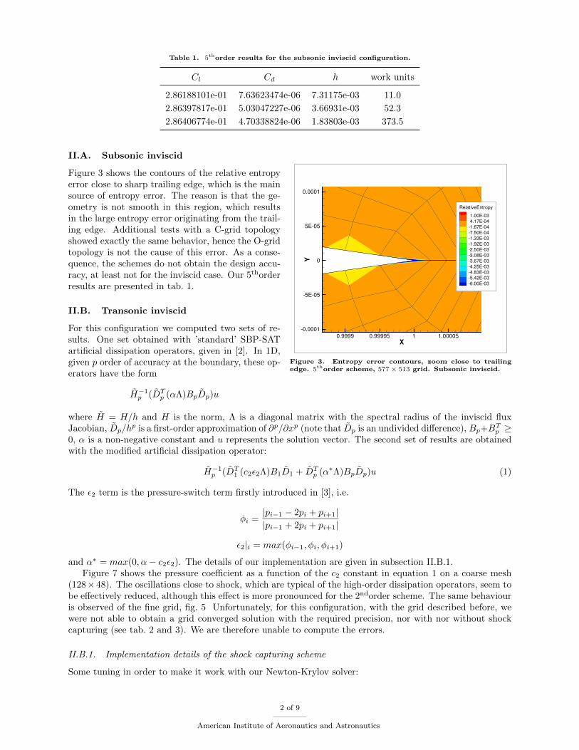
Table 1. 5thorder results for the subsonic inviscid configuration.

Cl Cd h work units

2.86188101e-01 7.63623474e-06 7.31175e-03 11.0

2.86397817e-01 5.03047227e-06 3.66931e-03 52.3

2.86406774e-01 4.70338824e-06 1.83803e-03 373.5

II.A. Subsonic inviscid

X

Y

0.9999 0.99995 1 1.00005

0.0001

5E05

0

5E05

0.0001

RelativeEntropy

1.00E03

4.17E04

1.67E04

7.50E04

1.33E03

1.92E03

2.50E03

3.08E03

3.67E03

4.25E03

4.83E03

5.42E03

6.00E03

Figure 3. Entropy error contours, zoom close to trailingedge. 5thorder scheme, 577× 513 grid. Subsonic inviscid.

Figure 3 shows the contours of the relative entropyerror close to sharp trailing edge, which is the mainsource of entropy error. The reason is that the ge-ometry is not smooth in this region, which resultsin the large entropy error originating from the trail-ing edge. Additional tests with a C-grid topologyshowed exactly the same behavior, hence the O-gridtopology is not the cause of this error. As a conse-quence, the schemes do not obtain the design accu-racy, at least not for the inviscid case. Our 5thorderresults are presented in tab. 1.

II.B. Transonic inviscid

For this configuration we computed two sets of re-sults. One set obtained with ’standard’ SBP-SATartificial dissipation operators, given in [2]. In 1D,given p order of accuracy at the boundary, these op-erators have the form

H−1p (DTp (αΛ)BpDp)u

where H = H/h and H is the norm, Λ is a diagonal matrix with the spectral radius of the inviscid fluxJacobian, Dp/h

p is a first-order approximation of ∂p/∂xp (note that Dp is an undivided difference), Bp+BTp ≥

0, α is a non-negative constant and u represents the solution vector. The second set of results are obtainedwith the modified artificial dissipation operator:

H−1p (DT1 (c2ε2Λ)B1D1 + DT

p (α∗Λ)BpDp)u (1)

The ε2 term is the pressure-switch term firstly introduced in [3], i.e.

φi =|pi−1 − 2pi + pi+1||pi−1 + 2pi + pi+1|

ε2|i = max(φi−1, φi, φi+1)

and α∗ = max(0, α− c2ε2). The details of our implementation are given in subsection II.B.1.Figure 7 shows the pressure coefficient as a function of the c2 constant in equation 1 on a coarse mesh

(128× 48). The oscillations close to shock, which are typical of the high-order dissipation operators, seem tobe effectively reduced, although this effect is more pronounced for the 2ndorder scheme. The same behaviouris observed of the fine grid, fig. 5 Unfortunately, for this configuration, with the grid described before, wewere not able to obtain a grid converged solution with the required precision, nor with nor without shockcapturing (see tab. 2 and 3). We are therefore unable to compute the errors.

II.B.1. Implementation details of the shock capturing scheme

Some tuning in order to make it work with our Newton-Krylov solver:

2 of 9


(a) 2ndorder scheme (b) 5thorder scheme

Figure 4. Transonic inviscid: Pressure coefficient profiles obtained with different values of the artificial dissipationconstant c2 (equation 1), coarse grid. The black line corresponds to c2 = 0, i.e. no shock capturing.

Figure 5. Transonic inviscid: Pressure coefficient profiles on the fine grid with c2 = 2.0 (equation 1), 2ndto 5thorderscheme.

X

Y

0.2 0 0.2 0.4 0.6 0.8 1 1.2

0

0.5

Pressure

1.50

1.41

1.32

1.23

1.14

1.05

0.96

0.87

0.78

0.69

0.60

(a) Pressure contours

X

Y

0.2 0 0.2 0.4 0.6 0.8 1 1.2

0

0.5

RelativeEntropy

1.50E02

1.30E02

1.10E02

9.00E03

7.00E03

5.00E03

3.00E03

1.00E03

2.00E03

4.00E03

(b) Relative entropy error contours

Figure 6. Transonic inviscid: fine grid results with shock capturing (c2 = 2.0), 5thorder scheme.

3 of 9


Table 2. 5thorder results for the transonic inviscid configuration, without shock capturing.

Cl Cd h work units

3.51991e-01 2.26498e-02 7.31175e-03 11.7

3.51682e-01 2.26161e-02 3.66931e-03 97.5

3.51607e-01 2.26216e-02 1.83803e-03 1425.6

Table 3. 5thorder results for the transonic inviscid configuration, with shock capturing.

Cl Cd h work units

3.48051e-01 2.28588e-02 7.31175e-03 31.8

3.51929e-01 2.26727e-02 3.66931e-03 212.3

3.51717e-01 2.26320e-02 1.83803e-03 1742.3

• φi is slightly different, it is computed as

φi =

[|pi−1 − 2pi + pi+1|

|pi−1 + 2pi + pi+1 + plim|

]1.1with plim = 0.001p∞

• ε2 = max(ε2, 0.25)

• α∗ is blended close to zero to avoid the clipping of the max function.

α∗ =

α− c2ε2 if (α− c2ε2) ≥ a

a2 − b(α− c2ε2)

(−b+ 2a)− (α− c2ε2)if (α− c2ε2) < a

with a = 1.e− 5 and b = 1.e− 12. a is where the blending begins and b is the asymptotic value whenc2ε2 →∞.

• ε2 is frozen after 2 non-linear iterations, and the whole non-linear system is solved twice to machineprecision.

The last modification turned out to be the most important one for stability: freezing the scheme was theonly way to obtain a converged solution.

II.C. Subsonic viscous

This configuration was assumed to have a steady-state solution which has been sought using both a (implicit)Newton-Krylov and a (explicit) Runge-Kutta solver with local time stepping. However, with the sharptrailing edge geometry, we found that only the former gave a steady state solution (shown in fig. 7(a)) whilethe latter was not able to find this solution; in fact the explicit Runge-Kutta solver did not converge. We alsocomputed a time-accurate solution using a third order ESDIRK scheme: we found a steady-state solutionwith the requested accuracy of 1.e− 6, albeit after very long integration time (> 60 convective times) beforewhich vortex shedding was observed, fig. 7(b). With a rounded trailing edge, all algorithms converged to asteady-state solution.

Unfortunately, for this configuration too, lift and drag do not exhibit a monotonic convergence with the5thorder scheme. The the only exception is the lift with the sharp trailing edge. However, we did obtain a’converged’ value with an accuracy of 1.e− 6 for both lift and drag on both geometries, as shown in tables 4and 5.

A. Background information for the SBP-SAT scheme

As is well-known, stability of a numerical scheme is a key property for a robust and accurate numericalsolution. Proving stability for high-order finite-difference schemes on bounded domains is a highly non-trivial task. One successful way to obtain stability proofs is to employ so-called Summation-by-Parts (SBP)

4 of 9


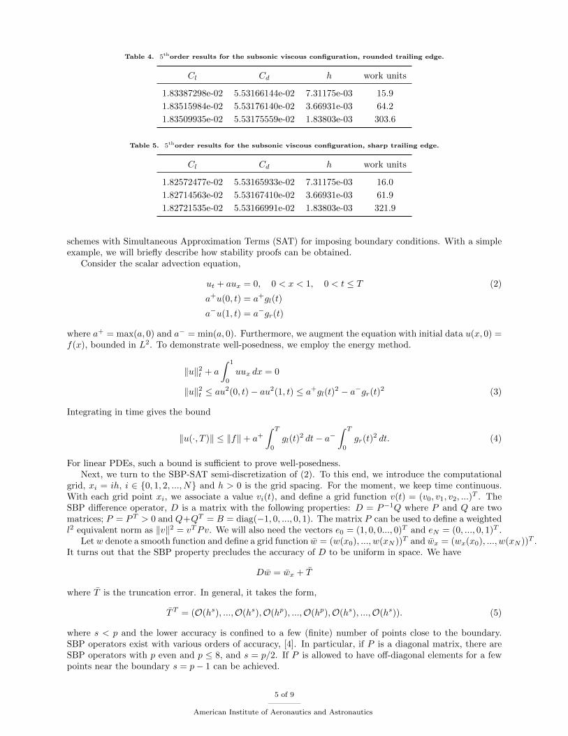
Table 4. 5thorder results for the subsonic viscous configuration, rounded trailing edge.

Cl Cd h work units

1.83387298e-02 5.53166144e-02 7.31175e-03 15.9

1.83515984e-02 5.53176140e-02 3.66931e-03 64.2

1.83509935e-02 5.53175559e-02 1.83803e-03 303.6

Table 5. 5thorder results for the subsonic viscous configuration, sharp trailing edge.

Cl Cd h work units

1.82572477e-02 5.53165933e-02 7.31175e-03 16.0

1.82714563e-02 5.53167410e-02 3.66931e-03 61.9

1.82721535e-02 5.53166991e-02 1.83803e-03 321.9

schemes with Simultaneous Approximation Terms (SAT) for imposing boundary conditions. With a simpleexample, we will briefly describe how stability proofs can be obtained.

Consider the scalar advection equation,

ut + aux = 0, 0 < x < 1, 0 < t ≤ T (2)

a+u(0, t) = a+gl(t)

a−u(1, t) = a−gr(t)

where a+ = max(a, 0) and a− = min(a, 0). Furthermore, we augment the equation with initial data u(x, 0) =f(x), bounded in L2. To demonstrate well-posedness, we employ the energy method.

‖u‖2t + a

∫ 1

0

uux dx = 0

‖u‖2t ≤ au2(0, t)− au2(1, t) ≤ a+gl(t)2 − a−gr(t)2 (3)

Integrating in time gives the bound

‖u(·, T )‖ ≤ ‖f‖+ a+∫ T

0

gl(t)2 dt− a−

∫ T

0

gr(t)2 dt. (4)

For linear PDEs, such a bound is sufficient to prove well-posedness.Next, we turn to the SBP-SAT semi-discretization of (2). To this end, we introduce the computational

grid, xi = ih, i ∈ {0, 1, 2, ..., N} and h > 0 is the grid spacing. For the moment, we keep time continuous.With each grid point xi, we associate a value vi(t), and define a grid function v(t) = (v0, v1, v2, ...)

T . TheSBP difference operator, D is a matrix with the following properties: D = P−1Q where P and Q are twomatrices; P = PT > 0 and Q+QT = B = diag(−1, 0, ..., 0, 1). The matrix P can be used to define a weightedl2 equivalent norm as ‖v‖2 = vTPv. We will also need the vectors e0 = (1, 0, 0..., 0)T and eN = (0, ..., 0, 1)T .

Let w denote a smooth function and define a grid function w = (w(x0), ..., w(xN ))T and wx = (wx(x0), ..., w(xN ))T .It turns out that the SBP property precludes the accuracy of D to be uniform in space. We have

Dw = wx + T

where T is the truncation error. In general, it takes the form,

TT = (O(hs), ...,O(hs),O(hp), ...,O(hp),O(hs), ...,O(hs)). (5)

where s < p and the lower accuracy is confined to a few (finite) number of points close to the boundary.SBP operators exist with various orders of accuracy, [4]. In particular, if P is a diagonal matrix, there areSBP operators with p even and p ≤ 8, and s = p/2. If P is allowed to have off-diagonal elements for a fewpoints near the boundary s = p− 1 can be achieved.

5 of 9


Using the SBP operators, we now define a semi-discrete scheme for (2).

vt + aDv = σla+P−1e0(v0 − gl(t)) + a−σrP

−1eN (vN − gr(t))

The right-hand side are the SAT:s, which impose the boundary conditions weakly. (Originally proposed in[5].) σl,r are two scalar parameters, to be determined by the stability analysis. Multiplying by 2vTP , weobtain

‖v‖2t − a(v20 − v2N ) = 2σla+v0(v0 − gl(t)) + 2a−σrvN (vN − gr(t))

(6)

For stability, it is sufficient to obtain a bound with gl,r = 0. In that case, it is easy to see that we mustrequire σl ≤ −1/2 and σr ≥ 1/2 to obtain a bounded growth of ‖v‖. More generally, allowing boundary datato be inhomogeneous when deriving a bound leads to strong stability. (See [6]. The benefit of proving strongstability as opposed to stability is that less regularity in the boundary data is required.) For strong stability,it can be shown that σl,r must satisfy σl < −1/2 and σr < 1/2, i.e., strict inequalities. As an example, thechoice σl = −1, σr = 1 leads to

‖v‖2t − a(v20 − v2N ) = −2a+v0(v0 − gl(t)) + 2a−vN (vN − gr(t))

or

‖v‖2t ≤ −a+(v0 − g)2 + a+gl(t)2 + a−(vN − gr(t)2)− a−g2 (7)

If v0 = gl, vN = gr, (7) is the same as (3), but this is not the case and the additional terms add a smalldamping to the boundary. Upon integration of (7) in time, an estimate corresponding to (4) is obtained. Wealso remark that the SAT terms are accurate as they do not contribute to a truncation error in the scheme.Furthermore, semi-discrete stability guarantees stability of the fully discrete problem obtained by employingRunge-Kutta schemes in time, [7].

The above example, demonstrates the general procedure for obtaining energy estimates for an SBP-SATscheme. Naturally, for systems of PDEs, in 3-D with stretched and curvilinear multi-block grids, and withadditional parabolic terms, the algebra for proving stability becomes more involved. However, the resultingschemes are still fairly straightforward to use. For the linearized Euler and Navier-Stokes equations, semi-discrete energy estimates have been derived. (See [8–10] and references therein.) Different boundary types,including far-field, walls and grid block interfaces are included in the theory. For flows with smooth solutions,linear stability implies convergence as the grid size vanishes. (See [11].)

B. Code description

Both a general code and specialized codes for some of the test cases (used in the 1st and 2nd high orderworkshop, see [12]) are available. The general code is a 3D code that can handle multiblock grids and canrun on (massively) parallel platforms. For load balancing reasons the blocks are split during runtime in anarbitrary number of sub-blocks with a halo treatment of the newly created interfaces, such that the resultsare identical to the sequential algorithm.

The specialized codes assume a single block 2D grid and do not have parallel capabilities, hence they arerelatively easy to modify for testing purposes. Due to the fact that these codes can only be used for onespecific test case and the fact that the general purpose code can only handle 3D problems, the efficiency ofthe specialized codes is quite a bit higher than the general purpose code.

The discretization schemes used are finite difference SBP-SAT schemes, see section A, of order 2 to 5.Thanks to the energy stability property of these schemes no or a significantly reduced amount of artificialdissipation is needed compared to schemes which do not posses this (or a similar) property. This leads to ahigher accuracy of the numerical solutions.

For the steady test cases the set of nonlinear algebraic equations is solved using the nonlinear solverlibrary of PETSc [13]. This library requires the Jacobian matrix of the spatial residual, which is computedvia dual numbers [14] and appropriate coloring of the vertices of the grid, for which the PETSc routines areused. Initial guesses are obtained via grid sequencing, where appropriate. The solution of the linear systemsneeded by PETSc’s nonlinear solution algorithm is obtained by Block ILU preconditioned GMRES.

6 of 9


Implicit time integration schemes of the ESDIRK type [15] are available, for which the resulting nonlinearsystems are solved using a slightly adapted version of the steady state algorithm explained above. However,for the unsteady test cases considered, the Euler vortex and the Taylor-Green vortex, the time steps neededfor accuracy are relatively small compared to the stability limit of explicit time integration schemes andtherefore the explicit schemes are better suited for these cases. The available explicit schemes are theclassical 4th order Runge Kutta scheme (RK4, [16]) and TVD Runge Kutta schemes up till 3rd order [17].As the maximum CFL number of the RK4 scheme is significantly higher than the CFL number of the TVDRunge Kutta schemes, the RK4 scheme is used for the unsteady test cases mentioned above.

For the post processing standard commercially available software, such as Tecplot, and open-sourcesoftware, such as Gnuplot, are used. Grid adaption has not been carried out.

C. Machines description

The results for the easy test cases have been obtained on a Linux work station running Ubuntu 10.04with an Intel i7-2600 CPU running at 3.4 GHz, with 8 Mb of cache. The machine contains 16 Gb of RAMmemory with an equivalent amount of swap. Running the Taubench on this machine led to a CPU time of5.59 seconds (average over 4 runs).

The difficult test cases were run on up to 512 processors on the LISA machine of SARA, the DutchSupercomputing Center and Hexagon, the Cray XE6 machine of the University of Bergen. Running theTaubench on these machines led to a CPU time of 10.3 and 10.8 seconds respectively (average over 4 runs).

References

1 “Pointwise User Manual,” Tech. rep., www.pointwise.com, 2011.

2 Mattsson, K., Svard, M., and Nordstrom, J., “Stable and Accurate Artificial Dissipation,” Journal ofScientific Computing , Vol. 21(1), August 2004, pp. 57–79.

3 Jameson, A., Schmidt, W., and Turkel, E., “Numerical solution of the Euler equations by finite volumemethods using Runge-Kutta time stepping schemes,” AIAA Paper 81-1259 , 1981.

4 Strand, B., “Summation by Parts for Finite Difference Approximations for d/d x,” J. Comput. Phys.,Vol. 110, 1994.

5 Carpenter, M. H., Gottlieb, D., and Abarbanel, S., “Time-stable boundary conditions for finite-differenceschemes solving hyperbolic systems: Methodology and application to high-order compact schemes,” J.Comput. Phys., Vol. 111(2), 1994.

6 Gustafsson, B., Kreiss, H.-O., and Oliger, J., Time dependent problems and difference methods, JohnWiley & Sons, Inc., 1995.

7 Kreiss, H.-O. and Wu, L., “On the stability definition of difference approximations for the initial boundaryvalue problem,” Applied Numerical Mathematics, Vol. 12, 1993, pp. 213–227.

8 Svard, M., Carpenter, M., and Nordstrom, J., “A stable high-order finite difference scheme for thecompressible Navier-Stokes equations, far-field boundary conditions,” Journal of Computational Physics,Vol. 225, 2007, pp. 1020–1038.

9 Svard, M. and Nordstrom, J., “A stable high-order finite difference scheme for the compressible Navier-Stokes equations, no-slip wall boundary conditions,” J. Comput. Phys., Vol. 227, 2008, pp. 4805–4824.

10 Nordstrom, J., Gong, J., van der Weide, E., and Svard, M., “A stable and conservative high ordermulti-block method for the compressible Navier-Stokes equations,” J. Comput. Phys., Vol. 228, 2009,pp. 9020–9035.

11 Strang, G., “Accurate partial difference methods II. Non-linear problems,” Num. Math., Vol. 6, 1964,pp. 37–46.

7 of 9


12 van der Weide, E., Giangaspero, G., and Svard, M., “Efficiency Benchmarking of an Energy StableHigh-Order Finite Difference Discretization,” AIAA Journal , 2015, doi: 10.2514/1.J053500.

13 Balay, S., Brown, J., Buschelman, K., Eijkhout, V., Gropp, W., Kaushik, D., Knepley, M., McInnes,L. C., Smith, B., and H.Zhang, “PETSc Users Manual, Revision 3.2,” Tech. rep., Argonne NationalLaboratory, 2011.

14 Fike, J. A., Jongsma, S., Alonso, J., and v.d. Weide, E., “Optimization with Gradient and HessianInformation Calculated Using Hyper-Dual Numbers,” AIAA paper 2011-3807 , 2011.

15 Kennedy, C. and Carpenter, M. H., “Additive Runge-Kutta schemes for convection-diffusion-reactio equa-tions,” Applied Numerical Mathematics, Vol. 44, 2003, pp. 139–181.

16 Press, W. H., Teukolsky, S. A., Vetterling, W. T., and Flannery, B. P., Numerical Recipes: The Art ofScientific Computing , Cambridge University Press, 3rd ed., 2007.

17 Gottlieb, S., Shu, C. W., and Tadmor, E., “High order time discretizations with strong stability property,”SIAM Review , Vol. 43, 2001, pp. 89 – 112.

8 of 9


X

Y

0 0.5 1 1.5 2 2.5 3

1.5

1

0.5

0

0.5

1

1.5

Mach

0.6

0.57

0.54

0.51

0.48

0.45

0.42

0.39

0.36

0.33

0.3

0.27

0.24

0.21

0.18

0.15

0.12

0.09

0.06

0.03

0

(a) Steady state solution obtain with the Newton-Krylovsolver.

X

Y

0 0.5 1 1.5 2 2.5 3

1.5

1

0.5

0

0.5

1

1.5

Mach

0.6

0.57

0.54

0.51

0.48

0.45

0.42

0.39

0.36

0.33

0.3

0.27

0.24

0.21

0.18

0.15

0.12

0.09

0.06

0.03

0

(b) Instantaneous solution obtained with the third orderESDIRK scheme before the shedding is damped out.

Figure 7. Mach contours, 5thorder scheme, fine grid, sharp trailing edge.

9 of 9


Case C1.2: Flow over the NACA0012 airfoil · Case C1.2: Flow over the NACA0012 airfoil Giorgio...

Documents

Transcript of Case C1.2: Flow over the NACA0012 airfoil · Case C1.2: Flow over the NACA0012 airfoil Giorgio...