Cascades on interdependent networks - Cornell …cpss/2012/dsouzaTalk2.pdfatP ! 0.05 before...
39
Cascades on interdependent networks Raissa M. D’Souza University of California, Davis Dept of CS, Dept of Mech. and Aero. Eng. Complexity Sciences Center External Professor, Santa Fe Institute
Transcript of Cascades on interdependent networks - Cornell …cpss/2012/dsouzaTalk2.pdfatP ! 0.05 before...

Cascades on interdependent networks
Raissa M. D’SouzaUniversity of California, Davis
Dept of CS, Dept of Mech. and Aero. Eng.Complexity Sciences Center
External Professor, Santa Fe Institute

A collection of interacting , dynamic networks
form the core of modern society
Networks:
TransportationNetworks/Power grid(distribution/collection networks)
Biological networks- protein interaction- genetic regulation- drug design
Computernetworks
Social networks- Immunology- Information- Commerce
E-commerce → WWW → Internet → Power grid → River networks.
Biological virus → Social contact network → Transportation nets →Communication nets → Power grid → River networks.

Critical infrastructure
From Peerenboom et. al.

Moving to systems of interdependent networksWhat are the simplest, useful, abstracted models?
What are the emergent new properties?– Host-pathogen interactions– Phase transition thresholds
What features confer resilience in one network whileintroducing vulnerabilities in others?
How do demands in one system shape the performance of theothers? (e.g., demand informed by social patterns ofcommunication)
How do constraints on one system manifest in others?(e.g., River networks shape placement of power plants)
Coupling of scales across space and time / co-evolution.

Configuration model for interacting networks
(E. Leicht and R. D’Souza, arXiv:0907.0894)
System of two networks Connectivity for an individual node
a
b
edges to aedges to b
• Degree distribution for nodes in network a: pakakb
• For the the system: {pakakb
, pbkakb}
• Generating functions to calculate properties of the ensemble ofsuch networks.

Modular Erdos-Renyi
Divide nodes initially into two groups (A and B):
A B
Add internal a-a edges with rate λ.
Add internal b-b edges with rate λ/r1, with r1 > 1.
Add intra-group a-b edges with rate λ/r2, with r2 > 1,r2 6= r1.
What happens? (Anything different?)

Wiring which respects group structures percolates earlier!
A B
1e+05 1e+06 1e+07 1e+08
0.82
0.86
n
k
S
k c0.
820.
86
1e+05 1e+06 1e+07 1e+08n
(Also tradeoffs between sparser and denser subnetworks.)
Probability distribution for node degrees: {pakakb , pbkakb}
Generating functions to calculate properties of the ensembleof such networks.

The flip side: “Catastrophic cascade of failures ininterdependent networks”
Buldyrev et. al. Nature 464 (2010).
Consider two coupled random graphs.
Nodes fail (removed either in a targeted or random manner).
Following an iterative removal process, small failures canlead to massive cascades of failure of the networks themselves.
Surprising: What confers resilience to individual network(broad-scale degree distribution) may be a weakness forrandomly coupled networks.

Single networks – broad scale degree distribution.
Illustration: Analysis of the Flight Weighted U.S. Air Transportation Network
! The flight weighted U.S. air
transportation network exhibits a
partial power law distribution
! Power law distribution for small and
medium size nodes up to approximately
250,000 flights per year
! Non power law distribution (above 250,000
flights per year)
! Hypothesis: Limits to scale and
capacitated nodes (i.e. capacity
constrained airports) are present in the non power law part of the distribution
10
U.S. Air Transportation Network(Airport level)
Analysis of the U.S. Air Transportation Network
*
Social contacts Airport trafficSzendroi and Csanyi Bounova 2009
We first identified protein classes significant-ly enriched or depleted in the high-confi-dence network (table S5). Enriched classesrelate primarily to DNA metabolism, tran-scription, and translation. Depleted classesare primarily plasma membrane proteins, in-cluding receptors, ion channels, and pepti-dases. Enrichment and depletion of specificclasses may be due to technical biases of thetwo-hybrid assay.
We then classified each interaction ac-cording to its corresponding pair of proteinclasses to identify class-pairs that are en-riched in the network. Rather than using acontingency table (13), we used a random-ization method to calculate statistical sig-nificance (6 ). Enriched class-pairs involv-ing structural domains (Pfam annotations)may represent binding modules and couldprovide the biological rules for buildingmultiprotein complexes. We identified 67pairs of Pfam domains enriched with a Pvalue of 0.05 or better after correcting formultiple testing (table S6). These includeknown domain pairs (F-box/Skp1, P ! 9 "10#20; LIM/LIM binding, P ! 5 " 10#8;actin/cofilin, P ! 2 " 10#7) as well asdomain pairs involving domains of un-known function (DUF227/DUF227, P !9 " 10#5; cullin/DUF298, P ! 0.0003). Anadditional 88 domain pairs are significantat P ! 0.05 before correcting for multipletesting and may represent additional bio-logically relevant binding patterns.Properties of the high-confidence pro-
tein-interaction network. Protein networksare of great interest as examples of small-world networks (14–16). Small-world net-works exhibit short-range order (two proteinsinteracting with a third protein have an en-hanced probability of interacting with eachother) but long-range disorder (two proteinsselected at random are likely to be connect-ed by a small number of links, as in arandom network).
Small-world properties arise in partfrom the existence of hub proteins, thosehaving many interaction partners. Hubs arecharacteristic of scale-free networks, andthe Drosophila network resembles a scale-free network in that the distribution of in-teractions per protein decays slowly, closeto a power law (Fig. 2D). To determine thesignature of biological organization insmall-world properties beyond what wouldbe expected of scale-free networks in gen-eral, we calculated properties for both theactual Drosophila network and an ensem-ble of randomly rewired networks with thesame distribution of interactions per proteinas in the original network. We consideredonly the giant connected component toavoid ill-defined mathematical quantities.
The distribution of the shortest path be-tween pairs of proteins peaks at 9 to 10
protein-protein links (Fig. 3A). A logistic-growth mathematical model for the probabil-ity that the shortest path between two distinctproteins has ! links is (N #1)#1 K$(!; N, J ),where K(!; N, J ) ! N/ [1% (N # 1) J#!] isthe number of proteins within ! links of acentral protein and the symbol $ indicatesdifferentiation with respect to !, K$(d; N,J ) ! N(N # 1)(ln J ) J#!/[1 % (N #1)J#!]2.Although this model fits the ensemble ofrandom networks, the fit to the actual net-work is less adequate.
Small-world properties of biologicalnetworks may reflect biological organiza-tion, and hierarchical organization has beenused to describe the properties of metabolicnetworks (7). We tested the ability of asimple, two-level hierarchical model to de-scribe the properties of the Drosphila pro-tein-interaction network. The lower level oforganization in this model represents pro-tein complexes, and the high level repre-sents interconnections of these complexes.In this case, the probability Pr(!) that the
Fig. 2. Confidence scores for protein-protein interactions (A) Drosophila protein-protein interac-tions have been binned according to confidence score for the entire set of 20,405 interactions(black), the 129 positive training set examples (green), and the 196 negative training set examples(red). (B) The 7048 proteins identified as participating in protein-protein interactions have beenbinned according to the minimum, average, and maximum confidence score of their interactions.Proteins with high-confidence interactions total 4679 (66% of the proteins in the network, and34% of the protein-coding genes in the Drosophila genome). (C) The correlation between GOannotations for interacting protein pairs decays sharply as confidence falls from 1 to 0.5, thenexhibits a weaker decay. Correlations were obtained by first calculating the deepest level in the GOhierarchy at which a pair of interacting proteins shared an annotation (interactions involvingunannotated proteins were discarded). The average depth was calculated for interactions binnedaccording to confidence score, with bin centers at 0.05, 0.1, . . . , 0.95. Finally, the correlation forthe bin centered at x was defined as [Depth(x) # Depth(0)]/[Depth(0.95) # Depth(0)]. Thisprocedure effectively controls for the depth of each hierarchy and for the probability that a pair ofrandom proteins shares an annotation. (D) The number of interactions per protein is shown for allinteractions (black circles) and for the high-confidence interactions (green circles). Linear behaviorin this log-log plot would indicate a power-law distribution. Although regions of each distributionappear linear, neither distribution may be adequately fit by a single power-law. Both may be fit,however, by a combination of power-law and exponential decay, Prob(n) & n#'exp#(n, indicatedby the dashed lines, with r 2 for the fit greater than 0.98 in either case (all interactions: ' ! 1.20)0.08, ( ! 0.038 ) 0.006; high-confidence interactions: ' ! 1.26 ) 0.25, ( ! 0.27 ) 0.05). Notethat the power-law exponents are within 1* for the two interaction sets.
R E S E A R C H A R T I C L E
www.sciencemag.org SCIENCE VOL 302 5 DECEMBER 2003 1729
on
Octo
be
r 5
, 2
00
9
ww
w.s
cie
nce
ma
g.o
rgD
ow
nlo
ad
ed
fro
m
Protein interactionsGiot et al Science 2003 (node degree)
Approximated as power law Pk ∝ k−γ

Pk ∼ k−γ, the first two moments
(Note: γ > 1 required for∑
k Pk = 1)
First moment (Mean degree):
〈k〉 =∞∑k=1
kpk ≈∫ ∞k=1
kpkdk
Diverges (i.e., 〈k〉 → ∞) if γ ≤ 2.
Second moment:
⟨k2⟩
=∞∑k=1
k2pk ≈∫ ∞k=1
k2pkdk
Diverges (i.e.,⟨k2⟩→∞) if γ ≤ 3.
Many results follow for 2 < γ < 3 since 〈k〉 /⟨k2⟩→ 0

Consequences of p(k) ∼ k−γ for networks
Most nodes are leaves (degree 1): Network connectivity veryrobust to random node removal.
High degree nodes are hubs: Network connectivity very fragileto targeted node removal.
letters to nature
NATURE | VOL 406 | 27 JULY 2000 | www.nature.com 379
called scale-free networks, which include the World-Wide Web3–5,the Internet6, social networks7 and cells8. We find that suchnetworks display an unexpected degree of robustness, the abilityof their nodes to communicate being unaffected even by un-realistically high failure rates. However, error tolerance comes at ahigh price in that these networks are extremely vulnerable toattacks (that is, to the selection and removal of a few nodes thatplay a vital role in maintaining the network’s connectivity). Sucherror tolerance and attack vulnerability are generic properties ofcommunication networks.
The increasing availability of topological data on large networks,aided by the computerization of data acquisition, had led to greatadvances in our understanding of the generic aspects of networkstructure and development9–16. The existing empirical and theo-retical results indicate that complex networks can be divided intotwo major classes based on their connectivity distribution P(k),giving the probability that a node in the network is connected to kother nodes. The first class of networks is characterized by a P(k)that peaks at an average !k" and decays exponentially for large k. Themost investigated examples of such exponential networks are therandom graph model of Erdos and Renyi9,10 and the small-worldmodel of Watts and Strogatz11, both leading to a fairly homogeneousnetwork, in which each node has approximately the same numberof links, k ! !k". In contrast, results on the World-Wide Web(WWW)3–5, the Internet6 and other large networks17–19 indicatethat many systems belong to a class of inhomogeneous networks,called scale-free networks, for which P(k) decays as a power-law,that is P!k""k! g, free of a characteristic scale. Whereas the prob-ability that a node has a very large number of connections (k q !k")is practically prohibited in exponential networks, highly connectednodes are statistically significant in scale-free networks (Fig. 1).
We start by investigating the robustness of the two basic con-nectivity distribution models, the Erdos–Renyi (ER) model9,10 thatproduces a network with an exponential tail, and the scale-freemodel17 with a power-law tail. In the ER model we first define the Nnodes, and then connect each pair of nodes with probability p. Thisalgorithm generates a homogeneous network (Fig. 1), whose con-nectivity follows a Poisson distribution peaked at !k" and decayingexponentially for k q !k".
The inhomogeneous connectivity distribution of many real net-works is reproduced by the scale-free model17,18 that incorporatestwo ingredients common to real networks: growth and preferentialattachment. The model starts with m0 nodes. At every time step t anew node is introduced, which is connected to m of the already-existing nodes. The probability !i that the new node is connectedto node i depends on the connectivity ki of node i such that!i # ki=Sjkj. For large t the connectivity distribution is a power-law following P!k" # 2m2=k3.
The interconnectedness of a network is described by its diameterd, defined as the average length of the shortest paths between anytwo nodes in the network. The diameter characterizes the ability oftwo nodes to communicate with each other: the smaller d is, theshorter is the expected path between them. Networks with a verylarge number of nodes can have quite a small diameter; for example,the diameter of the WWW, with over 800 million nodes20, is around19 (ref. 3), whereas social networks with over six billion individuals
Exponential Scale-free
ba
Figure 1 Visual illustration of the difference between an exponential and a scale-freenetwork. a, The exponential network is homogeneous: most nodes have approximatelythe same number of links. b, The scale-free network is inhomogeneous: the majority ofthe nodes have one or two links but a few nodes have a large number of links,guaranteeing that the system is fully connected. Red, the five nodes with the highestnumber of links; green, their first neighbours. Although in the exponential network only27% of the nodes are reached by the five most connected nodes, in the scale-freenetwork more than 60% are reached, demonstrating the importance of the connectednodes in the scale-free network Both networks contain 130 nodes and 215 links(!k " # 3:3). The network visualization was done using the Pajek program for largenetwork analysis: !http://vlado.fmf.uni-lj.si/pub/networks/pajek/pajekman.htm".
0.00 0.01 0.0210
15
20
0.00 0.01 0.020
5
10
15
0.00 0.02 0.044
6
8
10
12a
b c
f
d
Internet WWW
Attack
Failure
Attack
Failure
SFE
AttackFailure
Figure 2 Changes in the diameter d of the network as a function of the fraction f of theremoved nodes. a, Comparison between the exponential (E) and scale-free (SF) networkmodels, each containing N # 10;000 nodes and 20,000 links (that is, !k " # 4). The bluesymbols correspond to the diameter of the exponential (triangles) and the scale-free(squares) networks when a fraction f of the nodes are removed randomly (error tolerance).Red symbols show the response of the exponential (diamonds) and the scale-free (circles)networks to attacks, when the most connected nodes are removed. We determined the fdependence of the diameter for different system sizes (N # 1;000; 5,000; 20,000) andfound that the obtained curves, apart from a logarithmic size correction, overlap withthose shown in a, indicating that the results are independent of the size of the system. Wenote that the diameter of the unperturbed (f # 0) scale-free network is smaller than thatof the exponential network, indicating that scale-free networks use the links available tothem more efficiently, generating a more interconnected web. b, The changes in thediameter of the Internet under random failures (squares) or attacks (circles). We used thetopological map of the Internet, containing 6,209 nodes and 12,200 links (!k " # 3:4),collected by the National Laboratory for Applied Network Research !http://moat.nlanr.net/Routing/rawdata/". c, Error (squares) and attack (circles) survivability of the World-WideWeb, measured on a sample containing 325,729 nodes and 1,498,353 links3, such that!k " # 4:59.
© 2000 Macmillan Magazines Ltd
Epidemic spreading on the network (contact process):if 2 < γ < 3, then 〈k〉 /
⟨k2⟩→ 0 and limn→0 epidemic
threshold → 0.
(Buldyrev et al find broad scale more fragile for their particular cascade
dynamics)

Dynamical processes on interdependent networks
Motivation: interconnected power grids
C. Brummitt, R. M. D’Souza and E. A. Leicht PNAS 109 (12), 2012.
Power grid: a collectionof interdependent grids.(Interconnections built
originally for emergencies.)
Blackouts cascade fromone grid to another (in a
non-local manner).
Building moreinterconnections(Fig: planned windtransmission).Increasingly distributed Source: NPR
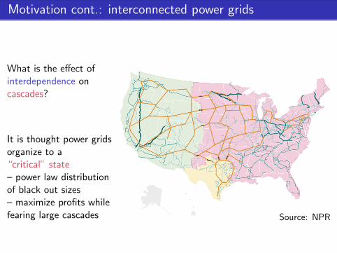
Motivation cont.: interconnected power grids
What is the effect ofinterdependence oncascades?
It is thought power gridsorganize to a“critical” state– power law distributionof black out sizes– maximize profits whilefearing large cascades Source: NPR

Sandpile models: “Self-organized criticality”
Drop grains of sand (“load”) randomly on nodes.
Each node has a threshold for sand.
Load > threshold node topples = sheds sand toneighbors.
These neighbors may topple. And their neighbors.And so on.
Cascades of load/stress on a system.
The classic Bak-Tang-Wiesenfeld sandpile model:(Neuronal avalanches, banking cascades, earthquakes, landslides, forest fires, blackouts...)
Finite square lattice in Z2
Thresholds 4
Open boundaries prevent inundation
Avalance size follows power law distribution P(s) ∼ s−3/2

Sandpile model on arbitrary networks
Sandpile model on arbitrary networks:
Thresholds = degrees(shed one grain per neighbor)
Boundaries: shedded sand are deletedindependently with probability f (:≈ 10/N)
Mean-field behavior (P(s) ∝ s−3/2) robust.(Goh et al. PRL 03, Phys. A 2004/2005, PRE
2005. PLRGs with 2 < γ < 3 not mean-field.)
Sandpiles on interacting networks:
Sparse connections between random graphs.
Configuration model with multi-type degreedistribution.
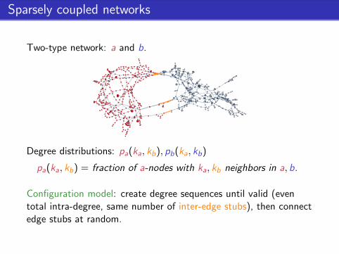
Sparsely coupled networks
Two-type network: a and b.
Degree distributions: pa(ka, kb), pb(ka, kb)
pa(ka, kb) = fraction of a-nodes with ka, kb neighbors in a, b.
Configuration model: create degree sequences until valid (eventotal intra-degree, same number of inter-edge stubs), then connectedge stubs at random.

Measures of avalanche size
• Topplings:Drop a grain of sand. How many nodes eventually topple?
Avalanche size distributions: sa(ta, tb), sb(ta, tb)
e.g., sa(ta, tb) = chance an avalanche begun in a topplesta many a-nodes, tb many b-nodes.
To study this, we need a more basic distribution...
• Sheddings: Drop a grain of sand. How many grains areeventually shed from one network to another?
Shedding size distributions: ρod(raa, rab, rba, rbb)= chance a grain shed from network o to d eventually causesraa, rab, rba, rbb many grains to be shed from a→a, a→b, b→a, b→b
*Approximate shedding and toppling as multi-type branchingprocesses.

Branching process approximation
Cascades in networks ≈ branching processes if they’re tree-like.
Power grids are fairly tree-like:clustering coefficient
Power grid in SE USA 0.01Similar Erdos-Renyi graph 0.001
(a)
(b)
(c)
(d)
(e)
Sandpile cascades on interacting networks ≈a multitype branching process.

Overview of the calculations
From degree distribution to avalanche size distribution:
Input: degree distributions pa(ka, kb), pb(ka, kb)
⇓ compute
shedding branching distributions qaa, qab, qba, qbb
⇓ compute
toppling branching distributions ua, ub
⇓ plug in
toppling branching generating functions Ua,Ub⇓ plug in
equations for avalanche size generating functions Sa,Sb⇓ solve numerically, asymptotically
Output: avalanche size distributions sa, sb

Shedding branch distribution, qod
Example:qab(rba, rbb) := the branch (children) distribution for
an ab-shedding .
Probability a single grain shed from a to b results in rbaa-sheddings and rbb b-sheddings.

Shedding branch distributions qodThe crux of the derivation
qod(rda, rdb) := chance a grain of sand shed from network o to dtopples that node, sending rda, rdb many grains to networks a, b.
qod(rda, rdb) =rdopd(rda, rdb)
〈kdo〉︸ ︷︷ ︸I
1
rda + rdb︸ ︷︷ ︸II
for rda + rdb > 0.
I: chance the grain lands on a node with degree pd(rda, rdb)(Edge following: rdo edges leading from network o.)
II: empirically, sand on nodes is ∼ Uniform{0, ..., k − 1}
Chance of no children = qod(0, 0) := 1−∑
rda+rdb>0 qod(rda, rdb)
(Probability a neighbor of any degree sheds, properly weighted.)
Chance at least one child = 1− qod(0, 0).

I. Edge following probability: single network
Degree distribution, Pk , with G.F. G0(x) =∑
k Pkxk .
Probability of following a random edge to a node of degree k :qk = kPk/
∑k kPk , with G.F. G1(x) =
∑k qkxk .
(“Contact immunization” strategy used by CDC.)
Generating function “self consistency” construction.H1(x): G.F. for dist in comp size following random edge
304 Generating functions formalism
reach it, is thus qk = (k +1)Pk+1/!k", and the corresponding generating function thereforereads
G1(x) =!
k
(k + 1)Pk+1
!k"xk = 1
!k"G #
0(x). (A2.5)
The definition and properties of generating functions allow us now to deal with theproblem of percolation in a random network: let us call H1(x) the generating functionfor the distribution of the sizes of the connected components reached by following arandomly chosen edge. Note that H1(x) considers only finite components and thereforeexcludes the possible giant cluster. We neglect the existence of loops, which is indeedlegitimate for such finite components. The distribution of sizes of such components canbe visualized by a diagrammatic expansion as shown in Figure A2.1: each (tree-like)component is composed by the node initially reached, plus k other tree-like components,which have the same size distribution, where k is the number of outgoing links of thenode, whose distribution is qk . The probability that the global component QS has size Sis thus
QS =!
k
qk Prob(union of k components has size S $ 1) (A2.6)
(counting the initially reached node in S). The generating function H1 is by definition
H1(x) =!
S
QS x S, (A2.7)
and the distribution of the sum of the sizes of the k components is generated by Hk1 (as
previously explained for the sum of degrees), i.e.!
S
Prob(union of k components has size S) · x S = (H1(x))k . (A2.8)
A
B
Fig. A2.1. Diagrammatic visualization of (A) Equation (A2.9) and (B) Equa-tion (A2.10). Each square corresponds to an arbitrary tree-like cluster, while thecircle is a node of the network.
H1(x) = xq0 + xq1H1(x) + xq2[H1(x)]2 + xq3[H1(x)]3 · · ·= xG1(H1(x))
(c.f. Newman, Strogatz, Watts PRE 2001.)

II. Revisiting the “1/k” assumption
Pierre-Andre Noel, C. Brummitt, R. D’Souzain progress
A node that just toppled isactually less likely to topple on
the next time step.(prob zero sand 6= 1/k)
The 1/k assumption for sandpiles on networks: origin, failure and alternative.Pierre-Andre Noel, Charles D. Brummitt, and Raissa M. D’Souza. University of California, Davis.
1. In a nutshell.
• A common assumption for sandpile models is shown to be false in quenched networks.
• This causes large deviations in the probability distribution.
• Previous work focused on power-law exponent, which is preserved.
• An alternative approach, based on self-consistency, is presented.
2. Context.
• We faced an unexpected problem while studying cascading
failures on power grids.
• We here study a minimal system reproducing the problem: a
Bak-Tang-Wiesenfeld sandpile model on a 3-regular network.
• The heterogeneous degree distribution case behaves similarly.
Size
0cascade.
Initialstate.
�
Size3cascade.
3. Sandpiles on 3-regular networks.
• Each node has up to 2 grains of sand on it.
• A new grain is dropped on a random node.
• Nodes with more than 2 grains topple:
their grains are sent to their neighbours.
• Sand is destroyed with probability �.
4. The 1/k assumption.
• Define pi the probability that a random node has i grains of sand on it.
• Define qij the probability that a node has j grains, knowing that its neighbour has i grains.
• The 1/k assumption states that the k nonzero pi are equal (i.e., p0 = p1 = p2 = 1/3).
• Christensen and Olami proved it for annealed networks (quenched case not proven).
– Annealed: a node’s neighbours are randomly chosen each time it topples.
– Quenched: neighbours at one time will always be neighbours (fixed structure).
• In quenched settings, it is often presented as an approximation (e.g., Goh et al.).
– Nodes topple 1/k of the times they receive a grain of sand (within 1%).
– Models using this assumption provide the right power-law exponent for cascade size.
• Hidden assumption: there are no correlations, i.e., qij = pj (true for annealed).
5. Failure of the 1/k assumption.
• For an infinite quenched network, a toppled node (parent) may only topple again during
the same cascade if all its neighbours (children) topple too: parent toppling is unlikely.
• Hence, more sand accumulates than in the annealed case (explaining p0 � 1/3).
• The process also introduces correlations (i.e., qij �= pj).
– For example, the only explanation for two neighbours to both have 0 grains on them is
that sand was destroyed when the last one toppled (explaining q00 � p0, since � is small).
6. Outline of the alternative approach.
• Treat the pi and qij as 12 unknown parameters.
– Normalization forces p0 + p1 + p2 = 1 and qi0 + qi1 + qi2 = 1.
– Network structure (and Bayes’ theorem) requires pi qij = pj qji.
– Hence, only 5 parameters are independent.
• Assumption: after some time, these parameters will reach a dynamical equilibrium.
• We consider a branching process providing the probability generating functionH(x,y, Z).
– x generates the cascade size distribution.
– yi generates the change in the number of nodes with i grains (and y = [y0 y1 y2]�).
– zij generates the change in the number of links joining nodes with i grains to nodes with
j grains (and Z is the matrix of these generators).
– Parent toppling is explicitly considered when all children topple.
• Fix the parameters by requesting self consistency.
– Constant pi implies no expected change in the number of nodes with i grains.
– Constant qij implies no expected change in the number of associated links.
0 =∂H
∂yi
����x=y
i�=zi�j�=1 ∀i�,j�0 =
∂H
∂zij
����x=y
i�=zi�j�=1 ∀i�,j�
Probability
Cascade size1 10 100 1000
10−2
10−3
10−4
10−5
10−6
Network of N = 4000 nodes.Using � = 0.01.
Slope −3/2.
Numerical simulations.
Using p2 = q22 = 1/3 (1/k assumption).
Using p2 = q22 = 1/2, parent cannot topple.
Figure: cascade size probability distribution as obtained through
numerical simulations (symbols) and analytical calculations (curves).
Red: the 1/k assumption fails at all scales to provide an accurate
probability distribution. Although it produces the right power-law
exponent, many similar assumptions do. Blue: making the approxi-
mation that parent nodes never topple, while other nodes topple 1/2
of the time they receive sand, is closer to reality.
p0 ≈ 0.091 q00 ≈ 0.005 q10 ≈ 0.071 q20 ≈ 0.116
p1 ≈ 0.337 q01 ≈ 0.262 q11 ≈ 0.319 q21 ≈ 0.359
p2 ≈ 0.573 q02 ≈ 0.733 q12 ≈ 0.611 q22 ≈ 0.525
Table: the actual pi and qij produced by the simulations.
p0 q300y1
y0
�z01z10
z00z00
�3
3 p0 q200 q01
y1
y0
�z01z10
z00z00
�2z11z11
z01z10
p1 q310y2
y1
�z02z20
z01z10
�3
3 p2 q320 �(1− �)2 x
y0
y2
�y1
y0
�2z00z00
z02z20
�z01z10
z02z20
�2· · ·
�
9p2q220q22(1− �)6x2
y1
y2
�y1
y0
�2y0
y2
�z11z11
z20z20
�2z01z10
z22z22· · ·
3p2q322�
2(1− �)13x5�y0
y2
�2�y1
y2
�2z00z00
z22z22
�z01z10
z22z22
�2· · ·
�
�
Above: some of the terms composing H(x,y, Z).
References.
- P. Bak, C. Tang, and K. Wiesenfeld. PRL 59, 381 (1987).- K. Christensen, and Z. Olami. PRE 48, 3361 (1993).- I. Dobson, B.A. Carreras, V.E. Lynch, and D.E. Newman. CHAOS 17, 026103 (2007).- K.-I. Goh, D.-S. Lee, B. Kahng, and D. Kim. PRL 91, 148701 (2003).
Acknowledgements.
- Defense Threat Reduction Agency, Basic Research Award HDTRA1-10-1-0088.- The Army Research Laboratory, Cooperative Agreement W911NF-09-2-0053.

Toppling branch distributions ua, ubshedding branch distributions qod toppling branch distributions ua, ub
Key: a node topples iff it sheds at least one grain of sand.
Probability an o to d shedding leads to at least one othershedding: 1− qod(0, 0). Probability a single shedding from ana-node yields ta, tb topplings:
ua(ta, tb) =∞∑
ka=ta,kb=tb
pa(ka, kb)Binomial [ta; ka, 1− qaa(0, 0)]·
· Binomial [tb; kb, 1− qab(0, 0)].
(e.g., ka neighbors, ta of them topple, each topples with prob
1− qaa(0, 0).)
Associated generating functions: Ua(τa, τb),Ub(τa, τb).

Summary of distributions and their generating functions
distribution generating function
degree pa(ka, kb), pb(ka, kb) Ga(ωa, ωb),Gb(ωa, ωb)
shedding branch qod(rda, rdb)
toppling branch ua(ta, tb), ub(ta, tb) Ua(τa, τb),Ub(τa, τb)
toppling size sa(ta, tb), sb(ta, tb) Sa(τa, τb),Sb(τa, τb)
Self-consistency equations:
Sa = τa Ua(Sa,Sb), (1)
Sb = τb Ub(Sa,Sb). (2)
Want to solve (1), (2) for Sa(τa, τb),Sb(τa, τb).Coefficients of Sa,Sb = avalanche size distributions sa, sb.
In practice, Eqs. (1), (2) are transcendental and difficult to invert.

Numerically solving ~S(~τ) = ~τ · ~U( ~S(~τ))
Methods for computing sa, sb for small avalanche size:
Method 1: Iterate starting from Sa = Sb = 1; expand.Method 2: Iterate symbolically; use Cauchy’s integration formula
sa(ta, tb) =1
(2πi)2
∫∫D
Sa(τa, τb)
τ ta+1a τ tb+1
b
dτadτb,
where D ⊂ C2 encloses the origin and no poles of Sa.Method 3: Multidimensional Lagrange inversion (IJ Good 1960):
Sa=∑∞
ma,mb=0
τmaa τ
mbb
ma!mb !
[∂ma+mb
∂κmaa ∂κ
mbb
{h(~κ)Ua(~κ)maUb(~κ)mb
∣∣∣∣∣∣∣∣δνµ− κµUµ ∂Uµ∂κµ
∣∣∣∣∣∣∣∣}]~κ=0
,
if the types µ, ν ∈ {a, b} have a positive chance of no children.
• Unfortunately for large avalanches need to use simulation.(Asymptotic approximations used for isolated networks do not apply.)

Plugging in degree distributions: A real world example
Two geographically nearby power grids in the southeastern US.
Grid c Grid d
# nodes 439 504
〈kint〉 2.4 2.9
〈kext〉 0.02 0.01
clustering 0.01 0.08
8 links between these two distinct grids.Different average internal degree 〈kint〉. Long paths.(Low clustering – approximately locally tree-like.)

A canonical idealization: Random regular graphs
Two random za-, zb-regular graphs with “Bernoulli coupling”:each node gets an external link independently with probability p.These ≈ power grids.
za = 3
zb = 4p = 0.1
Ua(τa, τb) =(p − pτa + (za + 1)(τa + za − 1))za(1 + p(τb − 1) + zb)
(za + 1)zazzaa (zb + 1)

Matching theory and simulation (for small’ish avalanches)
Plot marginalized avalanche size distributions
sa(ta) ≡∑tb≥0
sa(ta, tb), sa(tb) ≡∑ta≥0
sa(ta, tb), etc .
in simulations, branching process.
Regular(3)-Bernoulli(p)-Regular(10) Power grids c , d .

Main findings: For an individual network, optimal p∗
æ
æ
æ
æ
æ
ææ æ
æ
æ
æ
æ
ààà
à à àà à
à
à
à
à
ì
ìì
ì
ìì ì ì
ì
ì
ì
ì
0.1 0.2 0.3 0.4 0.5p
0.0002
0.0004
0.0006
0.0008
0.001
0.0012
0.0014
inflicted cascades
localcascades
p*
ì PrHTa>500Là PrHTba>500Læ PrHTaa>500L
• (Blue curve) Initially increasing p decreases the largest cascades startedin that network (second network is reservoir for load).
• (Red curve) Increasing p increases the largest cascades inflicted fromthe second network (two reasons: new channels and greater capacity).
• (Gold curve) Neglecting the origin of the cascade, the effects balance
at a stable critical point, p∗ ≈ 0.1. (Reduced by 75% from p=0.001 to p=0.1)
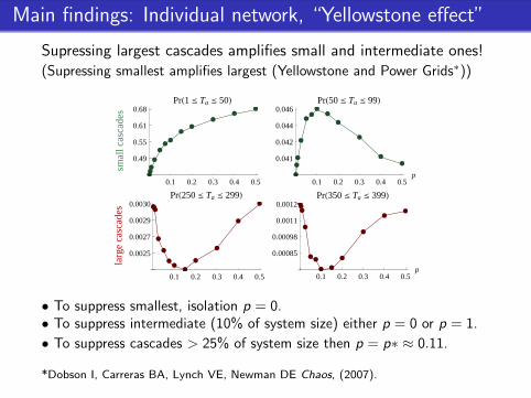
Main findings: Individual network, “Yellowstone effect”
Supressing largest cascades amplifies small and intermediate ones!(Supressing smallest amplifies largest (Yellowstone and Power Grids∗))
smal
lcas
cade
s
æææ
æ
æ
ææ
ææ
ææ
æ
0.1 0.2 0.3 0.4 0.5
0.49
0.55
0.61
0.68PrH1 £ Ta £ 50L
æ
æ
æ
æ
ææ
ææ
æ
æ
æ
æ
0.1 0.2 0.3 0.4 0.5p
0.041
0.042
0.044
0.046PrH50 £ Ta £ 99L
larg
eca
scad
es æææ
æ
æ
ææ
æ
æ
æ
æ
æ
0.1 0.2 0.3 0.4 0.5
0.0025
0.0027
0.0029
0.0030PrH250 £ Ta £ 299L
æææ
æ
ææ
æ æ
æ
æ
ææ
0.1 0.2 0.3 0.4 0.5p
0.00085
0.00098
0.0011
0.0012PrH350 £ Ta £ 399L
• To suppress smallest, isolation p = 0.• To suppress intermediate (10% of system size) either p = 0 or p = 1.
• To suppress cascades > 25% of system size then p = p∗ ≈ 0.11.
*Dobson I, Carreras BA, Lynch VE, Newman DE Chaos, (2007).

Main findings: System as a whole
More interconnections fuel larger system-wide cascades.
• Each new interconnection adds capacity and load to the system(Here capacity is a node’s degree, interconnections increase degree)
æ
æ
æ
æ
æ
ææ æ
æ
æ
æ
æ
ààà
à à àà à
à
à
à
à
ì
ìì
ì
ìì ì ì
ì
ì
ì
ì
0.1 0.2 0.3 0.4 0.5p
0.0002
0.0004
0.0006
0.0008
0.001
0.0012
0.0014
inflicted cascades
localcascades
p*
ì PrHTa>500Là PrHTba>500Læ PrHTaa>500L
• Test this on coupled random-regular graphs by rewiring internal edgesto be spanning edges (increase interconnectivity with out increasingdegree). No increase in the largest cascades.
• Inflicted cascades (Red curve) increase mostly due to increased capacity.
• So an individual operator adding edges to achieve p∗ may inadvertantly
cause larger global cascades.

Larger cascades from increased interconections:A warning sign?• Financial markets• Energy transmission systems
Source:
Technology Review,
“Joining the Dots”,
Jan/Feb (2011).

Main findings, continued: Frustrated equilibrium
Unless the coupled grids are identical, only one will be able toacheive it’s p∗.
Coupled za 6= zb regular random graphs (brancing process andsimulation).
〈sa〉b〈sb〉a
=1 + za1 + zb
If zb > za inflicted cascades from b to a larger than thosefrom a to b.
(An arm’s race for capacity?)

Summary: Sandpile cascades on interacting networks
Some interconnectivity can be beneficial, but too much isdetrimental. Stable optimal levels are possible.
From perspective of isolated network, seek optimalinterconnectivity p∗.
This equilibrium will be frustrated if the two networks differ intheir load or propensity to cascade.
Tuning p to suppress large cascades amplifies to occurrence ofsmall ones. (Likewise, suppressing small, amplifies large.)
Additional capacity and overall load from new interconnectionsfuels larger cascades in the system as a whole.
What might be good for an individual operator (adding edgesto achieve p∗), may be bad for society.

Possible extensions – Real power grids
Expand multi-typeprocesses to encode fordifferent types of nodes(buses, transformers,generators)
Linearized power flowequations – cascades inreal power grids arenon-local: e.g. fig: 3 to 4, 7 to 8
Game theoretic/economic consideration(we assume addingconnections is cost-free)
Sequence of outages in Western blackout, July 2 1996!
System Disturbances — 1996
NERC 26
Figure 1
from NERC 1996 blackout report!
(1996 Western blackout NERC report)
(Power grids as “critical” – Balancing profit and fear of outages)

Possible extensions
Teams and social networks
Tasks (sand) arriving on people (nodes)
Each person has a capacity for tasks: sheds once overloaded
Coupling to a second social network (team) can reduce largecascades
Amplifying cascades
Encourage adoption of new products
Snowball sampling
Airline networks
Different carriers accepting load (bumped passengers)

Other types of cascades, not just than sandpiles
Watt’s threshold model: “topple” is some fraction φ of yourneighbors have “toppled” (rather than “toppling”, Watt’sthink of cascades in adopting a new product).– Harder to “topple” nodes of high degree.
Kleinberg: rather than thresholds, diminishing returns(concave / sub-modular utility)

References and Acknowledgements
C. Brummitt, R. M. D’Souza and E. A. Leicht, “Suppressingcascades of load in interdependent networks”, it PNAS 109(12) 2012.
Note Author Summary for high-level overview.