Cary UV/Vis/NIR 5000 User Guide and Tutorial for Using the Cary 500

in the Reynolds Research Group

2nd Edition: April 2012

Georgia Institute of Technology School of Chemistry & Biochemistry

School of Materials Science and Engineering

Written by: Justin A. Kerszulis

Table of Contents

1. Introduction to the Cary 5000 ................................................................................................................ 3

1.1. Opening Remarks ............................................................................................................................... 3

1.2. Basics of Instrument and Software ............................................................................................. 3

2. Setting Up the Cary 5000 .......................................................................................................................... 6

2.1. Powering Up the Cary 5000 ........................................................................................................... 6

2.2. Sample Holders and Installing Sample Holders ..................................................................... 6

3. Experimental Setup .................................................................................................................................... 9

3.1. Preparing Samples for Solution Spectra ................................................................................... 9

3.2. Preparing Samples for Film Spectra ........................................................................................ 10

3.3. Preparing Samples for ITO to be Electrochemically Switched ...................................... 13

3.4. Setting Up the Software ................................................................................................................ 13

4. Data Acquisition ........................................................................................................................................ 17

4.1. Basic Data Acquisition without Electrochemistry.............................................................. 17

4.2. Spectroelectrochemistry .............................................................................................................. 23

5. Data Processing ......................................................................................................................................... 24

5.1. Converting Absorbance Data to Colorimetry ....................................................................... 24

1. Introduction to the Cary 5000

1.1. Opening Remarks

Welcome! This is the training manual for Agilent’s Cary 5000 UV/VIS/NIR spectrometer. This manual will introduce to you the basics on how to conduct the majority of all spectroscopic characterization in the Reynolds group. I hope this will be an enjoyable read for you.

The Cary is the workhorse of our group. It can be used to achieve simple solution or film spectra, fully characterize the switching window and spectral behavior of an electroactive polymer film (spectroelectrochemistry), the switching speed (chronoabsorptometry) of an electrochromic polymer film, temperature dependent spectra, and even colorimetry. Below are examples of each of the experiments mentioned.

[Images of basic solution or film spectra, spectroelectrochemistry, chronoabsorptometry, colorimetry from Cary, temp.depend spectra]

The above examples will be detailed in this manual. Using this manual, you will be able to attain all basic spectral characterization of your materials for use in publications and your graduation. This manual should be read in conjunction with the electrochemistry manual as most of the samples analyzed in this instrument will be electroactive materials.

1.2. Basics of Instrument and Software

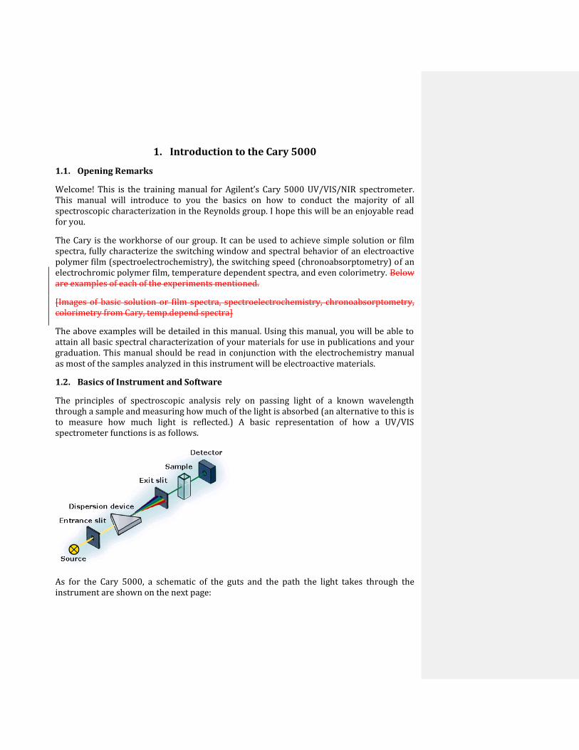
The principles of spectroscopic analysis rely on passing light of a known wavelength through a sample and measuring how much of the light is absorbed (an alternative to this is to measure how much light is reflected.) A basic representation of how a UV/VIS spectrometer functions is as follows.

As for the Cary 5000, a schematic of the guts and the path the light takes through the instrument are shown on the next page:

All of the necessary programs to run the characterizations are located on the Windows Desktop in the folder Cary WinUV as shown by the screen cap below.

In this folder are all the needed programs from running scans for spectroelectrochemistry to colorimetry, validation and maintenance, and a few VERY helpful…help files. The help files will go into more depth about not only the programs but the very scientific foundations of the instrument, accessories and experiments. The help files can also be accessed in each program.

As you perform more and more experiments on your ever expanding library of new materials, the number of files can get daunting and out of hand very quick. A good suggestion is to organize your files early on with meaningful file names sorted into folders. For example, you can make a new folder on the desktop and label it Polymer Films. Inside that folder can then be a subset of folders each referring to the material characterized. In those folders two new folders can then be created, one pertaining to the electrochemistry files performed by the CorrWare software and another containing all of the Cary files generated.

[Screencap of an example?]

2. Setting Up the Cary 5000

2.1. Powering Up the Cary 5000

Before you begin be sure to turn the Cary on: there is a power switch on the front, bottom left side which when turned on will be illuminated by a green light. Let the Cary warm up for about 30 minutes. This is so the lamp is putting out the maximum amount of light.

2.2. Sample Holders and Installing Sample Holders

There are a variety of sample holders we possess. We have a holder for cuvettes, a holder that is jacketed for cuvettes, (which allows thermal control of the cuvettes and for you to bathe the sample in an inert atmosphere), and there is a holder for glass slides as well.

[Pictures of the three holders]

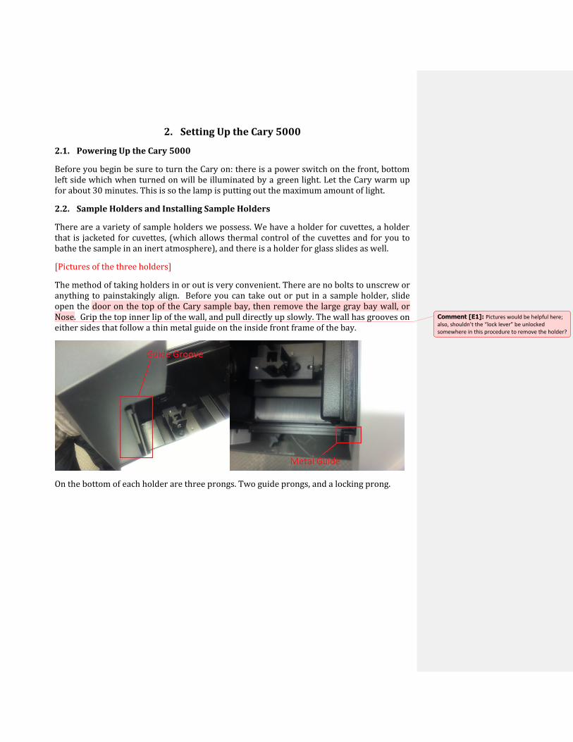
The method of taking holders in or out is very convenient. There are no bolts to unscrew or anything to painstakingly align. Before you can take out or put in a sample holder, slide open the door on the top of the Cary sample bay, then remove the large gray bay wall, or Nose. Grip the top inner lip of the wall, and pull directly up slowly. The wall has grooves on either sides that follow a thin metal guide on the inside front frame of the bay.

On the bottom of each holder are three prongs. Two guide prongs, and a locking prong.

Comment [E1]: Pictures would be helpful here; also, shouldn’t the “lock lever” be unlocked somewhere in this procedure to remove the holder?

These prongs slide in conveniently into the mounting and beam bay of the Cary which has the holes for the three prongs, shown below.

To place a cell holder in the bay, hold the plate by the handle so the prongs face down. Orient the plate so that to two guide prongs are facing into the bay. Tilt those prongs down at a slight angle and slowly push plate into the bay, and as the holder plate gets closer to the holes for the guide prongs, you can lower the plate so the prongs can touch the bay surface.

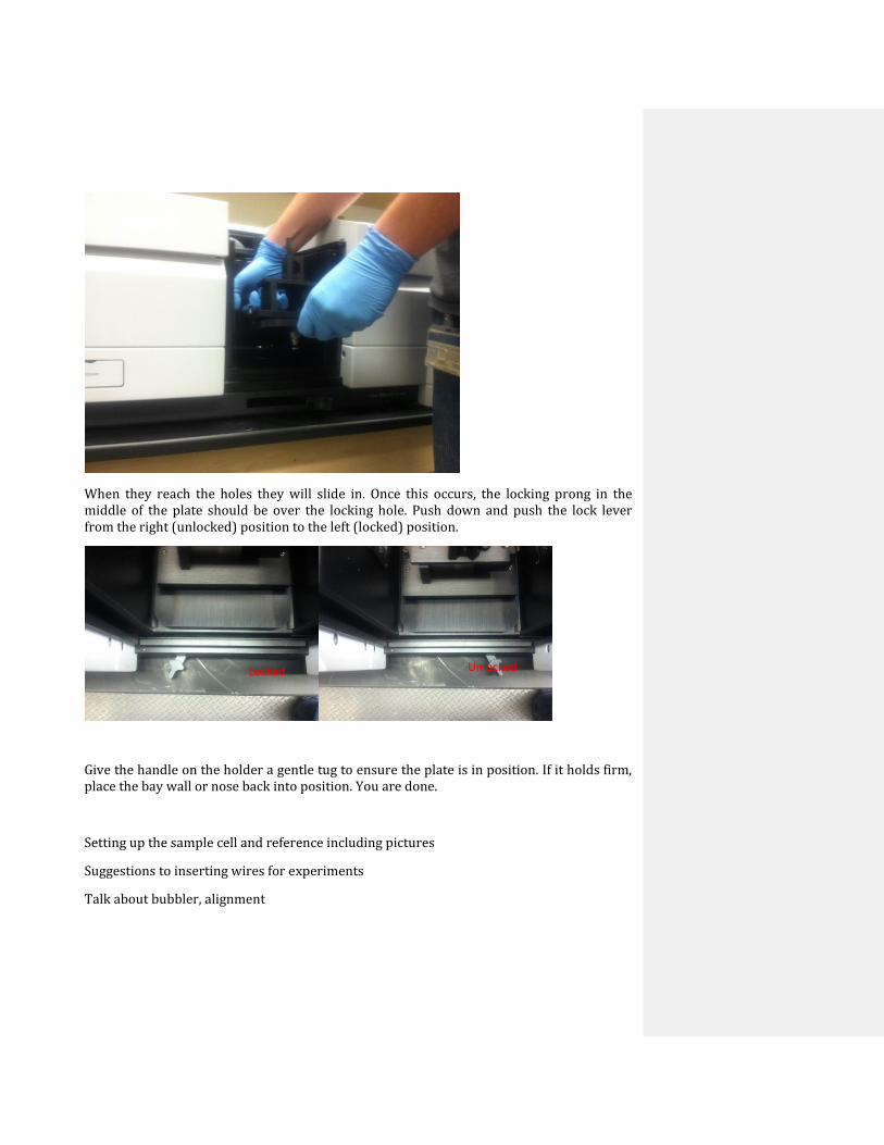
When they reach the holes they will slide in. Once this occurs, the locking prong in the middle of the plate should be over the locking hole. Push down and push the lock lever from the right (unlocked) position to the left (locked) position.

Give the handle on the holder a gentle tug to ensure the plate is in position. If it holds firm, place the bay wall or nose back into position. You are done.

Setting up the sample cell and reference including pictures

Suggestions to inserting wires for experiments

Talk about bubbler, alignment

Unlocked Locked

3. Experimental Setup

3.1. Preparing Samples for Solution Spectra

Solution spectroscopy is performed when you want to take the spectra of a sample dissolved in a solution. Samples are typically dilute, being on the order of less than 1mg/mL. The samples and blanks are to be prepared in small glass vials before being transferred into quartz cuvettes. Quartz cuvettes are used because glass would block the passage of light in the UV region. There are two types of these cuvettes. Two clear, two frosted sides, and all clear. If you use the two clear, two frosted version, ensure the clear sides are facing the beam. I think you know why.

While the Cary is warming up, prepare your samples. Below, in the left-hand photo is a padded box of clean cuvettes. You can acquire these from whoever is in charge of distributing electrochemistry supplies in our lab. The image on the right shows three samples we will use during this training exercise. The left and middle cuvette are both filled with 1:1 chloroform:toluene while the blue cuvette on the right contains two drops of a 2mg/mL of ECP-Cyan dissolved in a 1:1 chloroform:toluene solution.

You will use the dual cuvette plate and insert it into the Cary as described in the previous section. Of the two cuvette holders, the holder furthest inside the Cary is for a reference solution, which will remain there throughout the experiment; the holder closest to the front of the Cary is for establishing the blank baseline at the beginning of the experiment and for the sample itself later on.

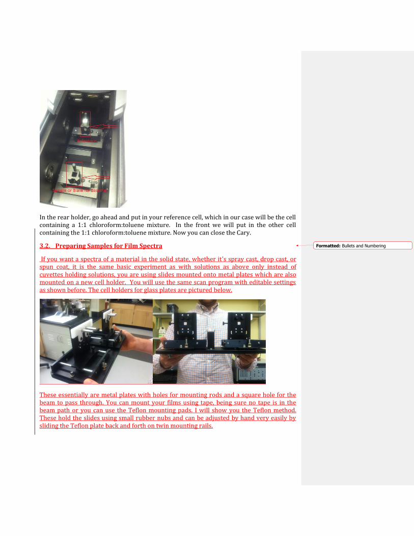
In the rear holder, go ahead and put in your reference cell, which in our case will be the cell containing a 1:1 chloroform:toluene mixture. In the front we will put in the other cell containing the 1:1 chloroform:toluene mixture. Now you can close the Cary.

3.2. Preparing Samples for Film Spectra

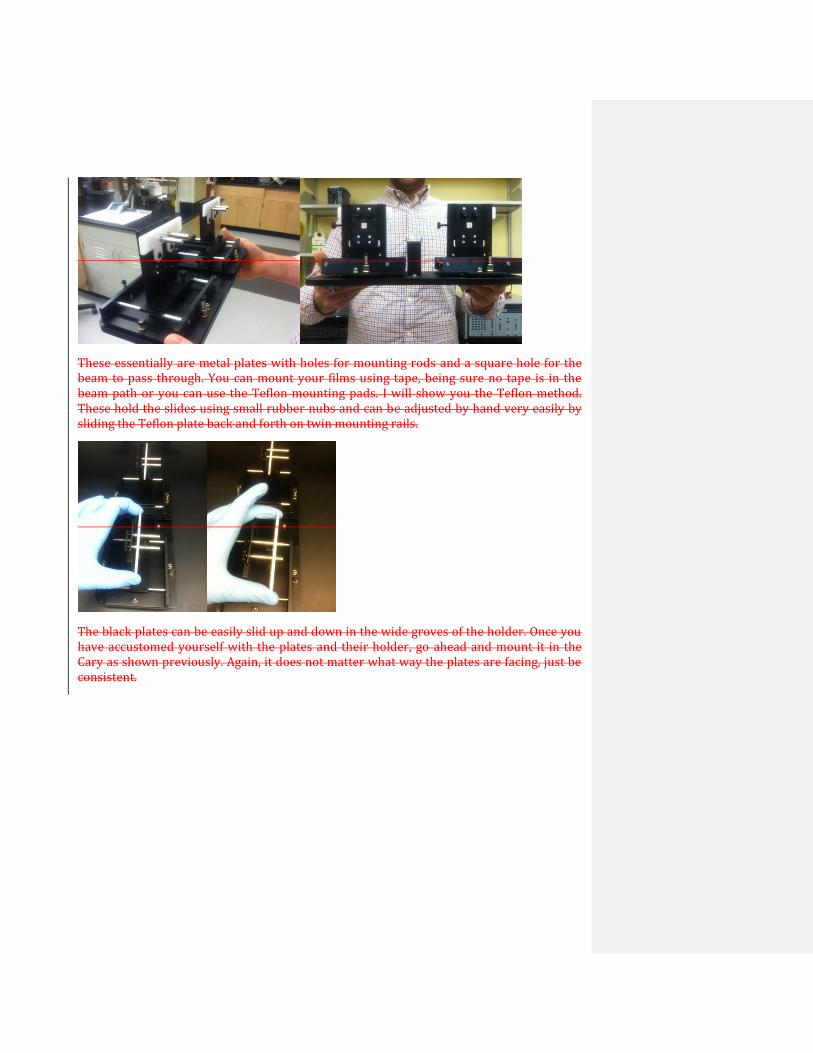
If you want a spectra of a material in the solid state, whether it’s spray cast, drop cast, or spun coat, it is the same basic experiment as with solutions as above only instead of cuvettes holding solutions, you are using slides mounted onto metal plates which are also mounted on a new cell holder. You will use the same scan program with editable settings as shown before. The cell holders for glass plates are pictured below.

These essentially are metal plates with holes for mounting rods and a square hole for the beam to pass through. You can mount your films using tape, being sure no tape is in the beam path or you can use the Teflon mounting pads. I will show you the Teflon method. These hold the slides using small rubber nubs and can be adjusted by hand very easily by sliding the Teflon plate back and forth on twin mounting rails.

Formatted: Bullets and Numbering

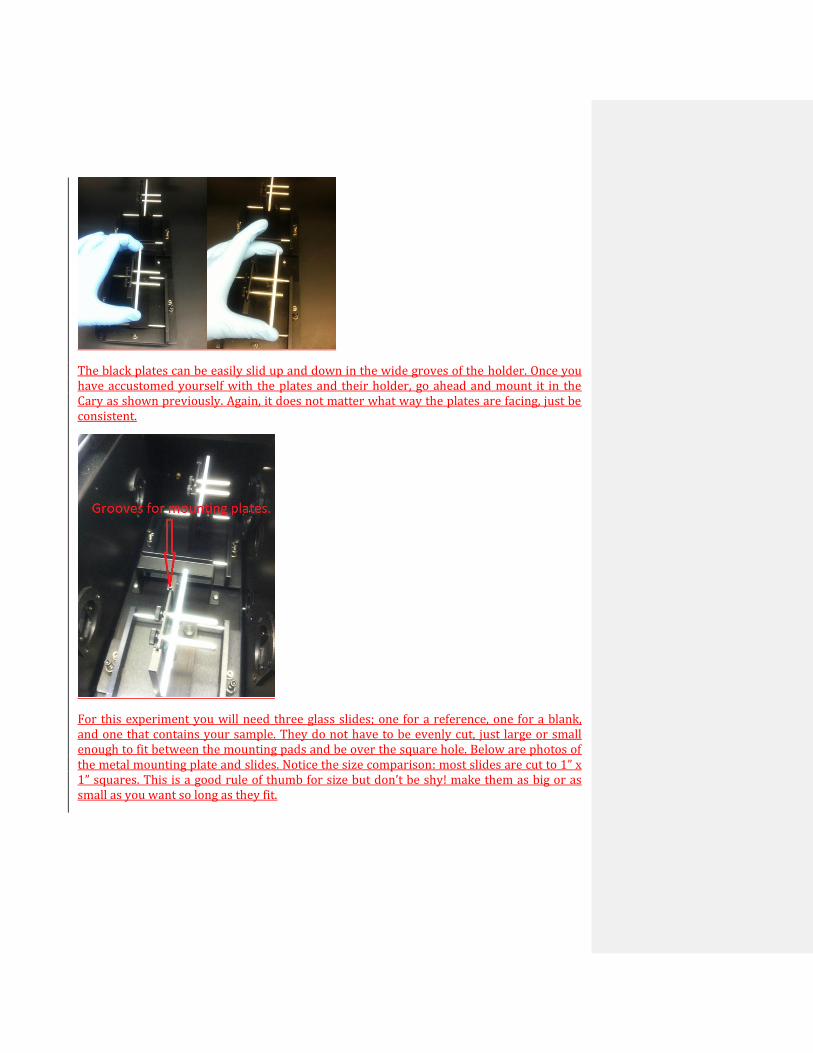
The black plates can be easily slid up and down in the wide groves of the holder. Once you have accustomed yourself with the plates and their holder, go ahead and mount it in the Cary as shown previously. Again, it does not matter what way the plates are facing, just be consistent.

For this experiment you will need three glass slides; one for a reference, one for a blank, and one that contains your sample. They do not have to be evenly cut, just large or small enough to fit between the mounting pads and be over the square hole. Below are photos of the metal mounting plate and slides. Notice the size comparison: most slides are cut to 1” x 1” squares. This is a good rule of thumb for size but don’t be shy! make them as big or as small as you want so long as they fit.

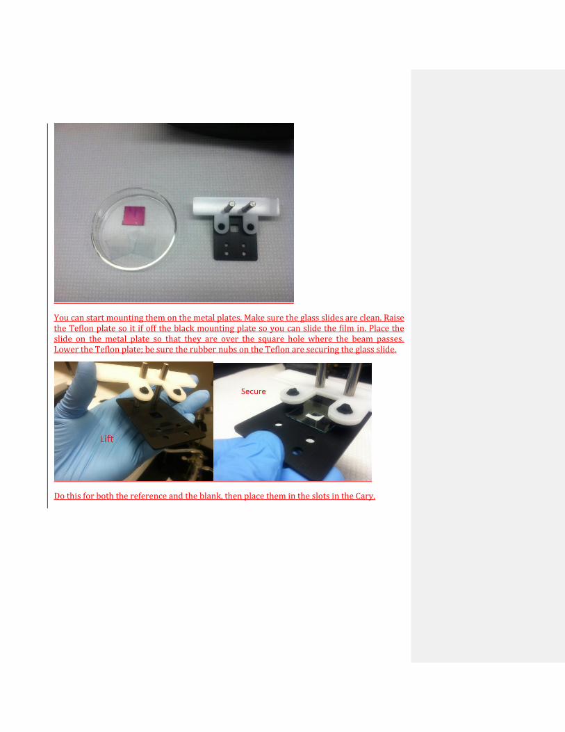
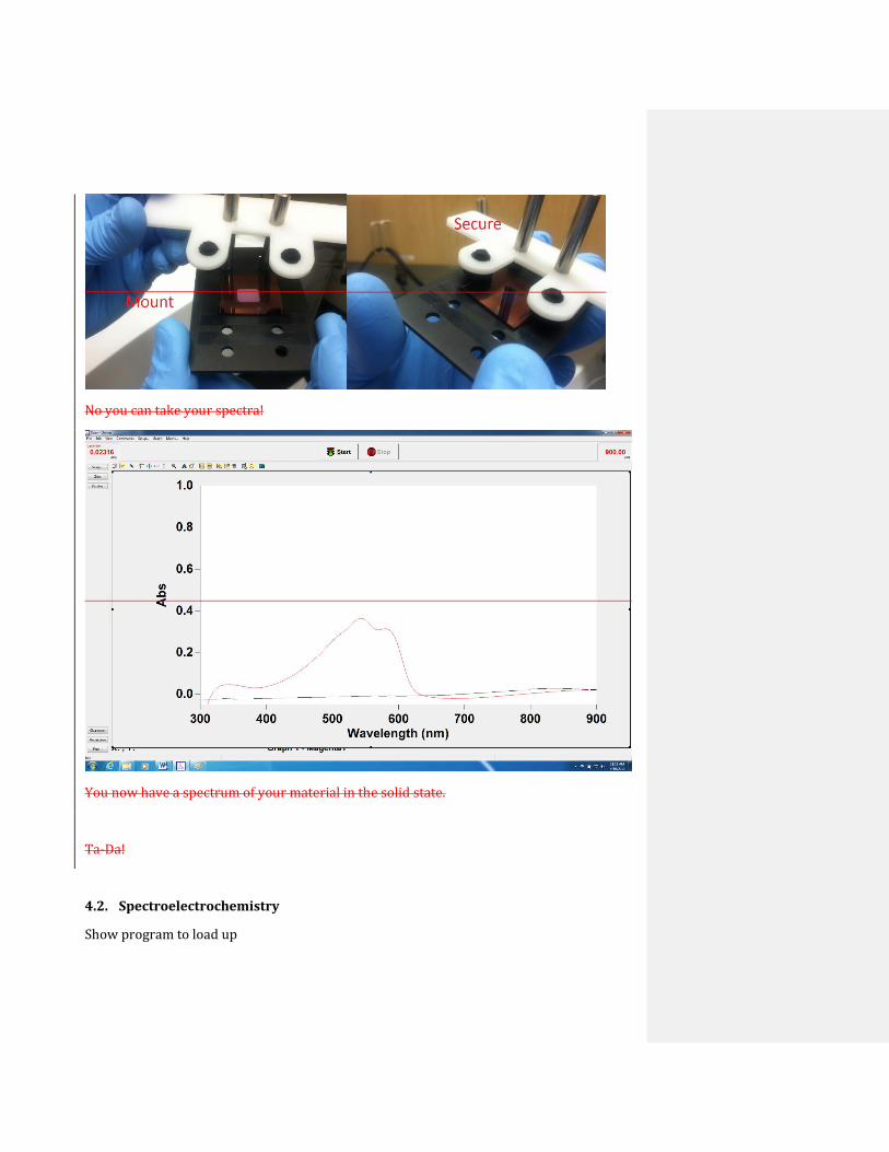
You can start mounting them on the metal plates. Make sure the glass slides are clean. Raise the Teflon plate so it if off the black mounting plate so you can slide the film in. Place the slide on the metal plate so that they are over the square hole where the beam passes. Lower the Teflon plate; be sure the rubber nubs on the Teflon are securing the glass slide.

Do this for both the reference and the blank, then place them in the slots in the Cary.

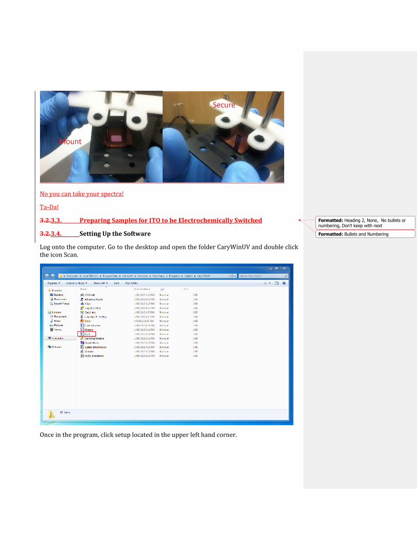
No you can take your spectra!

Ta-Da!

3.2.3.3. Preparing Samples for ITO to be Electrochemically Switched

3.2.3.4. Setting Up the Software

Log onto the computer. Go to the desktop and open the folder CaryWinUV and double click the icon Scan.

Once in the program, click setup located in the upper left hand corner.

Formatted: Heading 2, None, No bullets ornumbering, Don't keep with next

Formatted: Bullets and Numbering

You will be greeted with the setup window; here you can set your method for the coming experiments. The only tabs you will need to worry about for this experiment are Cary, Baseline, and Auto Store. When you click the Setup button, you will be automatically brought to the Cary tab as shown below.

In the X Mode section, this is where you setup the wavelength range for the Cary; in the Y Mode you set the absorption range (both can be changed to a variety of values appropriate to your experiment). The Cycle function allows you to run the same scan repeatedly, where

the Cycle Count controls the number of scans to be run, and the Cycle Time controls how long each cycle will take, which is both a combination of the time it takes to actually run a scan plus any desired lag time afterwards. This can be indirectly synchronized with a potentiostat to allow an entire spectroelectrochemical experiment to be run without an operator’s presence. This will be discussed later, but will not be needed for this experiment. Finally, under the Scan Controls section are options to control the rate that an individual scan is collected.

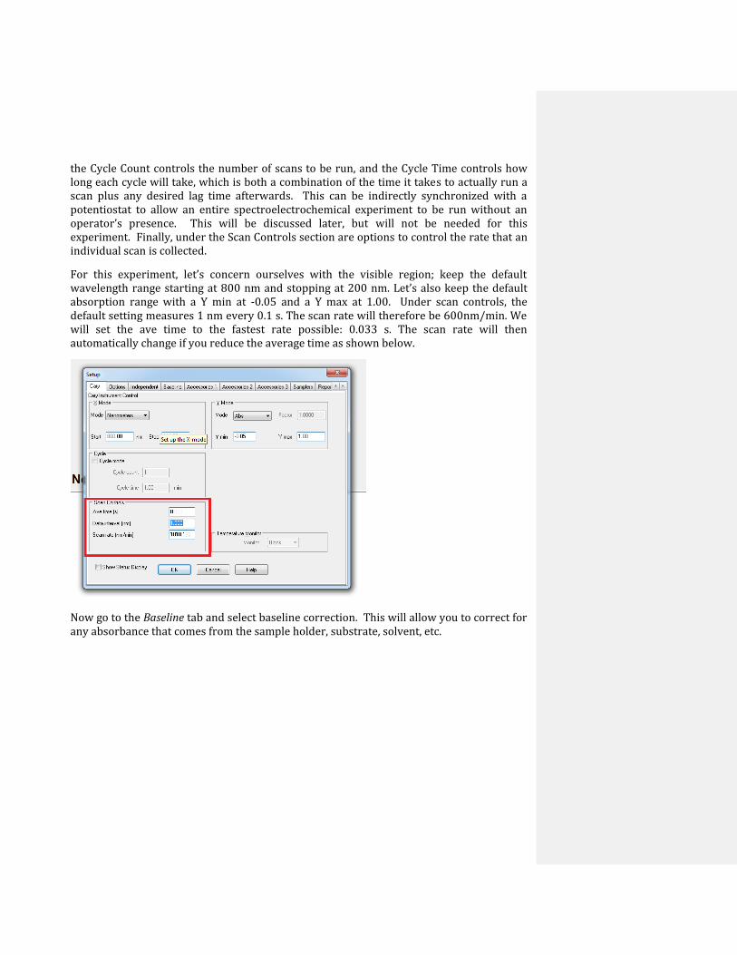
For this experiment, let’s concern ourselves with the visible region; keep the default wavelength range starting at 800 nm and stopping at 200 nm. Let’s also keep the default absorption range with a Y min at -0.05 and a Y max at 1.00. Under scan controls, the default setting measures 1 nm every 0.1 s. The scan rate will therefore be 600nm/min. We will set the ave time to the fastest rate possible: 0.033 s. The scan rate will then automatically change if you reduce the average time as shown below.

Now go to the Baseline tab and select baseline correction. This will allow you to correct for any absorbance that comes from the sample holder, substrate, solvent, etc.

Finally go to the Auto Store tab. Here you can have the Cary prompt you to save before a scan, after a scan or to never ask you to save. I recommend storage prompt at the start of an experiment, it keeps me organized. Click okay to close. This will be the method the experiment will use until you close the program, if you like it, you can save it by going to “file” then clicking “save method as”.

3.3.4. Data Acquisition

4.1. Basic Data Acquisition without Electrochemistry

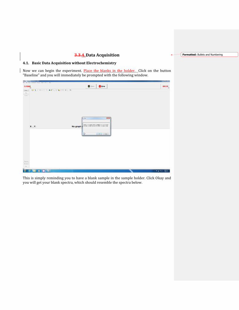
Now we can begin the experiment. Place the blanks in the holder. Click on the button “Baseline” and you will immediately be prompted with the following window.

This is simply reminding you to have a blank sample in the sample holder. Click Okay and you will get your blank spectra, which should resemble the spectra below.

Formatted: Bullets and Numbering

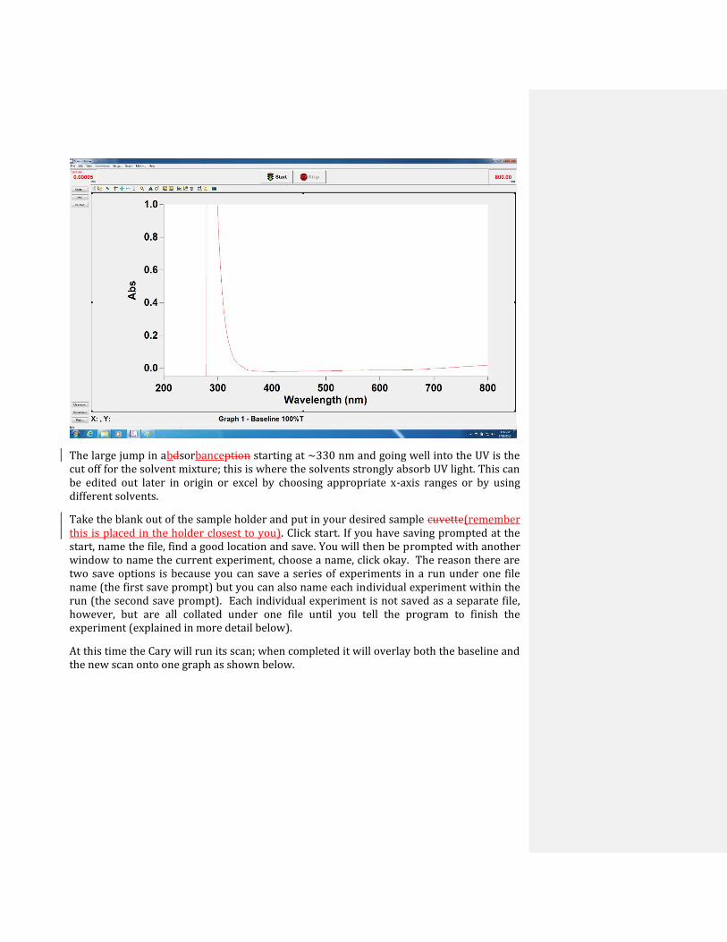
The large jump in abdsorbanception starting at ~330 nm and going well into the UV is the cut off for the solvent mixture; this is where the solvents strongly absorb UV light. This can be edited out later in origin or excel by choosing appropriate x-axis ranges or by using different solvents.

Take the blank out of the sample holder and put in your desired sample cuvette(remember this is placed in the holder closest to you). Click start. If you have saving prompted at the start, name the file, find a good location and save. You will then be prompted with another window to name the current experiment, choose a name, click okay. The reason there are two save options is because you can save a series of experiments in a run under one file name (the first save prompt) but you can also name each individual experiment within the run (the second save prompt). Each individual experiment is not saved as a separate file, however, but are all collated under one file until you tell the program to finish the experiment (explained in more detail below).

At this time the Cary will run its scan; when completed it will overlay both the baseline and the new scan onto one graph as shown below.

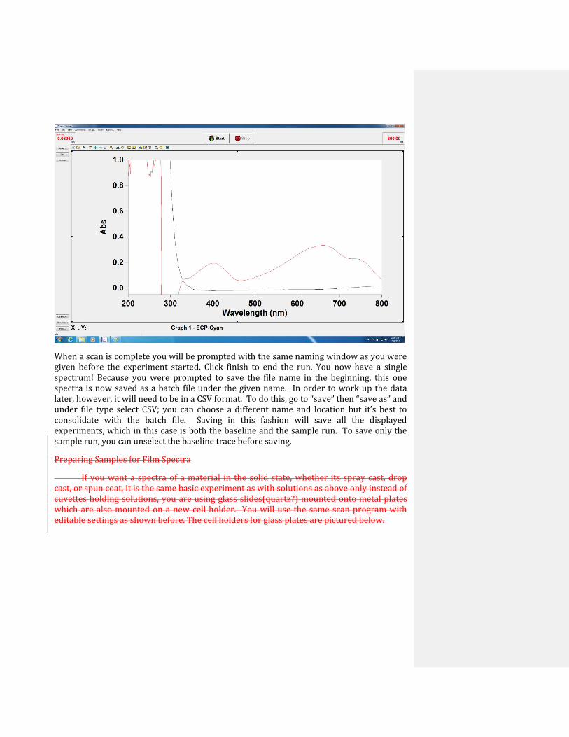
When a scan is complete you will be prompted with the same naming window as you were given before the experiment started. Click finish to end the run. You now have a single spectrum! Because you were prompted to save the file name in the beginning, this one spectra is now saved as a batch file under the given name. In order to work up the data later, however, it will need to be in a CSV format. To do this, go to “save” then “save as” and under file type select CSV; you can choose a different name and location but it’s best to consolidate with the batch file. Saving in this fashion will save all the displayed experiments, which in this case is both the baseline and the sample run. To save only the sample run, you can unselect the baseline trace before saving.

Preparing Samples for Film Spectra

If you want a spectra of a material in the solid state, whether its spray cast, drop cast, or spun coat, it is the same basic experiment as with solutions as above only instead of cuvettes holding solutions, you are using glass slides(quartz?) mounted onto metal plates which are also mounted on a new cell holder. You will use the same scan program with editable settings as shown before. The cell holders for glass plates are pictured below.

These essentially are metal plates with holes for mounting rods and a square hole for the beam to pass through. You can mount your films using tape, being sure no tape is in the beam path or you can use the Teflon mounting pads. I will show you the Teflon method. These hold the slides using small rubber nubs and can be adjusted by hand very easily by sliding the Teflon plate back and forth on twin mounting rails.

The black plates can be easily slid up and down in the wide groves of the holder. Once you have accustomed yourself with the plates and their holder, go ahead and mount it in the Cary as shown previously. Again, it does not matter what way the plates are facing, just be consistent.

For this experiment you will need three glass slides; one for a reference, one for a blank, and one that contains your sample. They do not have to be evenly cut, just car large or small enough to fit between the mounting pads and be over the square hole. Below are photos of the metal mounting plate and slides. Notice the size comparison. This is a good rule of thumb for size but don’t be shy! make them as big or as small as you want so long as they fit.

You can start mounting them on the metal plates. Make sure the glass slides are clean. Raise the Teflon plate so it if off the black mounting plate so you can slide the film in. Place the

slide on the metal plate so that they are over the square hole where the beam passes. Lower the Teflon plate; be sure the rubber nubs on the Teflon are securing the glass slide.

Do this for both the reference and the blank, then place them in the slots in the Cary, take your blank.

Remove the blank and insert your properly secured sample. Again be sure the sample is in the square and it is properly secured.

No you can take your spectra!

You now have a spectrum of your material in the solid state.

Ta-Da!

4.2. Spectroelectrochemistry

Show program to load up

Basic setup for experiment, include any normal noises heard or messages shown during setup

How to save setup as a method, what a method is

Slowly go over the experiment

How to save, what to save

5. Data Processing

5.1. Converting Absorbance Data to Colorimetry

The Cary is equipped with software that can take any acquired spectra and convert it into any needed form of colorimetry data. It allows you to easily switch through a variety of sources, observers, scales and much more! Detailed herein are the basic steps for converting your spectroelectrochemistry data in to an L*a*b* color plot.

From the desktop, open Cary WinUV and double click the Icon named Color as shown below. When in the program, click file, then click open data and find a spectra or batch file you wish to convert.

Once opened you will see the spectra you have taken earlier. On the lower left hand corner, there is a “recalculate” button. Click your spectra prior to pushing this button, this tells the program what graph you wish to convert. If you do not select a graph you will be greeted with a yellow caution window titled Recalculation Information with the message: “Make sure the scan graph is focused”, click okay and select a spectrum then try again.

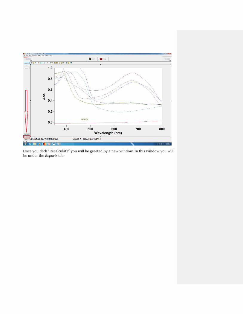
Once you click “Recalculate” you will be greeted by a new window. In this window you will be under the Reports tab.

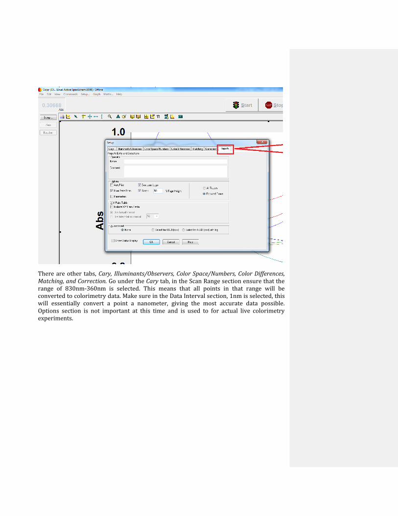
There are other tabs, Cary, Illuminants/Observers, Color Space/Numbers, Color Differences, Matching, and Correction. Go under the Cary tab, in the Scan Range section ensure that the range of 830nm-360nm is selected. This means that all points in that range will be converted to colorimetry data. Make sure in the Data Interval section, 1nm is selected, this will essentially convert a point a nanometer, giving the most accurate data possible. Options section is not important at this time and is used to for actual live colorimetry experiments.

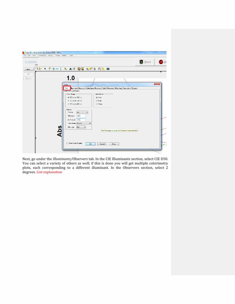
Next, go under the Illuminants/Observers tab. In the CIE Illuminants section, select CIE D50. You can select a variety of others as well; if this is done you will get multiple colorimetry plots, each corresponding to a different illuminant. In the Observers section, select 2 degrees. List explanation

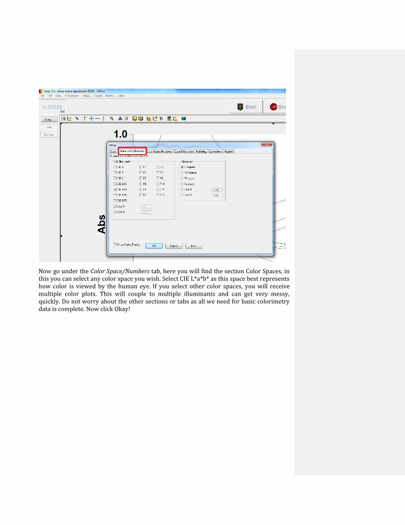
Now go under the Color Space/Numbers tab, here you will find the section Color Spaces, in this you can select any color space you wish. Select CIE L*a*b* as this space best represents how color is viewed by the human eye. If you select other color spaces, you will receive multiple color plots. This will couple to multiple illuminants and can get very messy, quickly. Do not worry about the other sections or tabs as all we need for basic colorimetry data is complete. Now click Okay!

Once you click okay, you will be greeted with an error tab Calculation range is bigger than continuum range. This can be because you have only have data shown from 400-800nm for example, smaller than the 360-850nm range you selected earlier. This is fine, click Okay. You will see a split screen, on the left, your original spectra, on the right a blank color space. To display your color plot, select the color space graph then click on the Trace Preferences Icon.

In the Visible tab, click the empty boxes to “check” them. Once all are checked, click Apply.

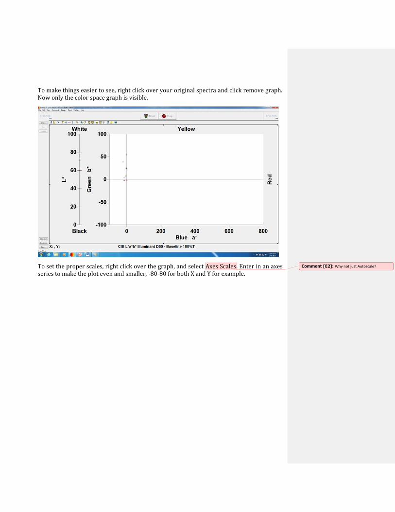
To make things easier to see, right click over your original spectra and click remove graph. Now only the color space graph is visible.

To set the proper scales, right click over the graph, and select Axes Scales. Enter in an axes series to make the plot even and smaller, -80-80 for both X and Y for example.

Comment [E2]: Why not just Autoscale?

Your color data is done. Saving will be addressed soon.

Chronoabsorptometry

Show program to load

Describe set up

Saving the method

Running the experiment

Saving the data

Temperature Dependent Experiments

Uses Scan

Same experimental setup at with Spectroelectrochem but emphasize the difference

Describe adjusting temperature from control box in conjunction with scans and Echem

Diffuse Reflectance

Detail the difference between using this method and others

Describe how to set the system up while describing particular functions of different pieces

Comment [E3]: For now just copy and paste into powerpoint presentations, etc.

Describe mirror alignment if needed

Entail how to perform the experiment

Deuterium Lamp Hydrogen Diffusion Test

Entail what this is for and what it means

Show where the file for the test is located

Entail how to run the test

How to interpret results

Closing Statement

Briefly state what they have read is for basic Cary use for the standard experiments we do

Detail some sources to look into

Emphasize a lot of the information here came from the Cary help tutorial