arX

iv:1

412.

4857

v2 [

mat

h.ST

] 2

1 Ja

n 20

16

The Annals of Statistics

2016, Vol. 44, No. 1, 401–424DOI: 10.1214/15-AOS1370c© Institute of Mathematical Statistics, 2016

A GOODNESS-OF-FIT TEST FOR STOCHASTIC BLOCK MODELS

By Jing Lei

Carnegie Mellon University

The stochastic block model is a popular tool for studying commu-nity structures in network data. We develop a goodness-of-fit test forthe stochastic block model. The test statistic is based on the largestsingular value of a residual matrix obtained by subtracting the es-timated block mean effect from the adjacency matrix. Asymptoticnull distribution is obtained using recent advances in random matrixtheory. The test is proved to have full power against alternative mod-els with finer structures. These results naturally lead to a consistentsequential testing estimate of the number of communities.

1. Introduction. Large-scale network data with community structureshave been the focus of much research efforts in the past decade [see, e.g.,Newman and Girvan (2004), Newman (2006)]. In the statistics and machinelearning literature, the stochastic block model (Holland, Laskey and Lein-hardt, 1983) is a very popular model for community structures in networkdata. In a stochastic block model, the observed network is often recorded inthe form of an n×n adjacency matrix A, representing the presence/absenceof pairwise interactions among n individuals in a population of interest. Themodel assumes that (i) the individuals are partitioned into K disjoint com-munities, and (ii) given the memberships, the upper diagonal entries of Aare independent Bernoulli random variables, where the parameter E(Aij)depends only on the memberships of nodes i and j. Such a model nat-urally captures the community structures commonly observed in complexnetworks, and has close connection to nonparametric exchangeable randomgraphs (Bickel and Chen, 2009). The stochastic block model can be mademore realistic by incorporating additional parameters to better approximatereal world network data. For example, Karrer and Newman (2011) incorpo-rated individual node activeness into the stochastic block model to allow

Received December 2014; revised August 2015.AMS 2000 subject classifications. 62H15.Key words and phrases. Network data, stochastic block model, goodness-of-fit test,

consistency, Tracy–Widom distribution.

This is an electronic reprint of the original article published by theInstitute of Mathematical Statistics in The Annals of Statistics,2016, Vol. 44, No. 1, 401–424. This reprint differs from the original in paginationand typographic detail.

1

2 J. LEI

for arbitrary degree distributions. In the mixed membership model (Airoldiet al., 2008), each individual may belong to more than one community.

In this paper, we develop a goodness-of-fit test for stochastic block models.Given an adjacency matrix A and a positive integer K0, we test whether Acan be adequately fitted by a stochastic block model with K0 communities.Our test statistic is the largest singular value of a residual matrix obtained byremoving the estimated block mean effect from the observed adjacency ma-trix. Intuitively, if A is generated by a stochastic block model and the blockmean effect is estimated appropriately, the residual matrix will approximatea generalized Wigner matrix: a symmetric random matrix with independentmean zero upper diagonal entries. Our first contribution is the asymptoticnull distribution of the test statistic (Theorem 3.1). The proof uses somerecent advances in random matrix theory, such as the local semicircle lawof generalized Wigner matrices and its consequences (Erdos, Yau and Yin,2012, Erdos et al., 2013a, Bloemendal et al., 2014). Our second contributionis asymptotic power guarantee of the test against models with finer struc-tures (Theorems 3.3 and 3.5). In particular, we establish the growth rateof the test statistic under alternatives that correspond to stochastic blockmodels with more communities or with individual node degree variations.It is of particular interest to consider alternative stochastic block modelswith more communities because any exchangeable random graph can be ap-proximated by a stochastic block model (Bickel and Chen, 2009). In oursimulation study, we observe that the proposed test is powerful against notonly stochastic block models with more communities, but also other networkmodels with finer structures such as the degree corrected block model andthe mixed membership block model.

A related test statistic using the largest eigenvalue of the centered andscaled adjacency matrix has been studied in Bickel and Sarkar (2013). Theyderive asymptotic null distribution for Erdos–Renyi models, which corre-sponds to a stochastic block model with one community. We generalize theirargument to prove the asymptotic null distribution result for stochastic blockmodels with more than one community. The key step is to bound the fluc-tuation in the leading eigenvalue of a random matrix under perturbationof a block-wise constant noise matrix. Moreover, their asymptotic poweranalysis requires the alternative model to be diagonal dominant. Our teststatistic uses the largest singular value of the residual matrix, so we are ableto capture signals affecting either the largest or the smallest eigenvalues, andour asymptotic power guarantee holds for a much wider class of alternativemodels.

Our goodness-of-fit test can also serve as a main building block to esti-mate the number of communities. As a key inference problem in stochasticblock models and its variants, the community recovery problem concerns

A GOODNESS-OF-FIT TEST FOR STOCHASTIC BLOCK MODELS 3

estimating the hidden communities from a single observed adjacency ma-trix [see McSherry (2001), Bickel and Chen (2009), Decelle et al. (2011),Zhao, Levina and Zhu (2012), Jin (2012), Fishkind et al. (2013), Lei andRinaldo (2013), Chen, Sanghavi and Xu (2012), Chaudhuri, Chung and Tsi-atas (2012), Krzakala et al. (2013), Massoulie (2013), Mossel, Neeman andSly (2013), Abbe, Bandeira and Hall (2014), Anandkumar et al. (2014),e.g.]. A common assumption made in all these methods is that K, the to-tal number of communities, is known. Therefore, estimating the number ofcommunities in a stochastic block model is of great practical and theoreti-cal importance. Some methods have been proposed to estimate the numberof communities in stochastic block models (Zhao, Levina and Zhu, 2011,Bickel and Sarkar, 2013, Chen and Lei, 2014, Saldana, Yi and Feng, 2014),but without consistency guarantee.

To estimate the number of communities, we consider hypothesis test

H0,K0 :K =K0, against Ha,K0 :K >K0(1)

sequentially for each K0 ≥ 1 until the null hypothesis is not rejected. Weprove the consistency of this sequential testing estimator in Corollary 3.4 ofSection 3. Throughout this paper, we use K to denote the true number ofcommunities in a stochastic block model and useK0 to denote a hypotheticalnumber of communities.

Recently, Chatterjee (2015) studied a general method for matrix denoisingusing singular value thresholding, which covers the stochastic block model asa special case. Following the ideas developed there, one may use the numberof significant singular values, for example, those greater than

√n, of the

adjacency matrix as an estimate of K. But this method only works whenthe community-wise connectivity matrix has full rank. Empirically, we alsofind that the sequential testing estimator developed in this paper performsbetter than singular value thresholding for sparse networks.

Glossary. For a square matrix M , diag(M) denotes the diagonal ma-trix induced by M . For any n × n symmetric matrix M , λj(M) denotesits jth largest eigenvalue value, ordered as λ1(M)≥ λ2(M)≥ · · · ≥ λn(M),and σ1(M) is the largest singular value. Denote BK the set of all K ×Ksymmetric matrices with entries in (0,1) and all rows being distinct.

2. Stochastic block models and a goodness-of-fit test. A stochastic blockmodel on n nodes with K communities is parameterized by a membershipvector g ∈ {1, . . . ,K}n and a symmetric community-wise edge probabilitymatrix B ∈ [0,1]K×K . The observed adjacency matrix A is a symmetricbinary matrix with diagonal entries being 0. Given (g,B), the probabilitymass function for the adjacency matrix A is

Pg,B(A) =∏

1≤i<j≤n

BAijgigj (1−Bgigj )

(1−Aij).(2)

4 J. LEI

In other words, given (g,B), the edges are independent Bernoulli randomvariables with parameters determined by the node memberships.

To avoid triviality, we say that a stochastic block model parameterized by(g,B) has K communities if (i) g contains all K distinct values in {1, . . . ,K},and (ii) any two rows of B are distinct. A stochastic block model is iden-tifiable up to a label permutation on g and a corresponding row/columnpermutation on B.

Given an observed adjacency matrix A, and a positive integer K0, wewould like to know if A can be well fitted by a stochastic block model withK0 communities. If we assume that A is generated by a stochastic blockmodel with K communities, this leads to a goodness-of-fit test for stochasticblock models with a composite null hypothesis

H0,K0 :K =K0.(3)

To derive a goodness-of-fit test for stochastic block models, a natural ideais to estimate the model parameters and remove the signal from the observedadjacency matrix, and test whether the residual matrix looks like a noisematrix. To this end, consider the n× n matrix P given by

Pij =Bgigj ,

so that E(A) = P − diag(P ). Let A∗ be

A∗ij =

Aij −Pij√

(n− 1)Pij(1−Pij), i 6= j and A∗

ii = 0,∀i.(4)

Then A∗ is a generalized Wigner matrix, satisfying E(A∗ij) = 0 for all (i, j)

and∑

j var(A∗ij) = 1 for all i. The asymptotic distribution of the extreme

eigenvalues of A∗ has been well studied in random matrix theory. In par-ticular, combining results in Erdos, Yau and Yin (2012) and Lee and Yin(2014) we have

n2/3[λ1(A∗)− 2] TW1 and n2/3[−λn(A∗)− 2] TW1,(5)

where TW1 denotes the Tracy–Widom distribution with index 1 and “ ”denotes convergence in distribution. We remark that (5) cannot be obtainedusing results for standard Wigner matrices as the diagonal entries of A∗

are fixed to be 0. We formally state and prove this result as Lemma A.1 inSection A.1.

The matrix A∗ involves unknown model parameters and cannot be usedas a test statistic. Now we describe a natural estimate of A∗ by plugging inan estimated stochastic block model.

Let g be an estimated community membership vector with target numberof communities being K0. Define Nk = {i : 1≤ i≤ n, gi = k}, and nk = |Nk|

A GOODNESS-OF-FIT TEST FOR STOCHASTIC BLOCK MODELS 5

for all 1≤ k ≤K0. We consider the plug-in estimator of B:

Bkl =

∑

i∈Nk,j∈NlAij

nknl, k 6= l,

∑

i,j∈Nk,i<jAij

nk(nk − 1)/2, k = l.

(6)

The estimates (g, B) leads to the empirically centered and re-scaled adja-cency matrix A:

Aij =

Aij − Pij√

(n− 1)Pij(1− Pij), i 6= j,

0, i= j,

(7)

where

Pij = Bgigj .(8)

It is natural to conjecture that under the null hypothesis K =K0 and whenthe estimates (g, B) are accurate enough, the convergence in (5) will carryover to the corresponding eigenvalues of A. Therefore, we can use the largestsingular value of A, after centering and scaling, as our test statistic:

Tn,K0 = n2/3[σ1(A)− 2].(9)

The corresponding level α rejection rule for testing problem (3) is

Reject H0,K0, if Tn,K0 ≥ t(α/2),(10)

where t(α/2) is the α/2 upper quantile of the TW1 distribution for α ∈ (0,1).We use t(α/2) instead of t(α) for Bonferroni correction because

σ1(A) =max(λ1(A),−λn(A)),

and hence

Tn,K0 =max[n2/3(λ1(A)− 2), n2/3(−λn(A)− 2)].

A similar result concerning the largest eigenvalue of A in the simple caseK0 = 1 has been obtained in Bickel and Sarkar (2013). In Section 3 below,we formally state and prove the validity of our test statistic Tn,K0 in Theo-rem 3.1 by establishing the asymptotic null distributions of both the largestand smallest eigenvalues and for general values of K0.

The use of σ1(A) instead of λ1(A) as our test statistic in (9) is crucialfor power guarantee. Under some alternative hypotheses, the signal may becarried solely by λn(A). For example, consider a model with two equal-sized

6 J. LEI

communities and B11 =B22 = 1/4, B12 =B21 = 1/2. Suppose we would like

to test H0 :K =K0 = 1. In this case, A− P has block-wise mean(

−1/8 1/81/8 −1/8

)

,

which has no positive eigenvalues. Therefore, the test using only λ1(A) hasno power.

Given the rejection rule (10) for testing problem (3), we have the followingsequential testing estimator of K:

K = inf{K0 ≥ 1 : Tn,K0 < tn}.(11)

In other words, we perform the goodness-of-fit test for K0 = 1,2, . . . , untilfailing to reject H0,K0 . We prove consistency of K for appropriate choices oftn in Corollary 3.4 below, as a consequence of (i) a large deviation inequalityof the extreme eigenvalues of A under the null hypothesis K =K0, and (ii)the growth rate of Tn,K0 under the alternative hypothesis K >K0.

3. Asymptotic null distribution and power. The asymptotic distribu-tion of the test statistic Tn,K0 under the null hypothesis depends on theaccuracy of the estimated community membership g. In order to considerthe asymptotic behavior of community recovery, we consider a sequence of

stochastic block models {(g(n),B(n)) : n≥ 1} where g(n) ∈ {1, . . . ,K(n)}n foreach n, and B(n) ∈ BK(n) . Here, the number of communities K =K(n) and

the community-wise edge probability matrix B =B(n) are allowed to changewith n.

We will focus on relatively balanced communities.

(A1) There exists c0 > 0 such that min1≤k≤K(n) |{i : g(n)i = k}| ≥ c0n/K(n)

for all n.

Assumption (A1) assumes each community has size at least proportional ton/K(n). For example, it is satisfied almost surely if the membership vectorg(n) is generated from a multinomial distribution with n trials and proba-bility π = (π1, . . . , πK(n)) such that min1≤k≤K πk > c0/K

(n) and K(n) growsslowly.

Definition (Consistency of community recovery). For a sequence of

stochastic block models {(g(n),B(n)) : n ≥ 1} with K(n) communities andB(n) ∈ BK(n) , we say a community membership estimator g = g(A,K(n)) isconsistent if

PA∼(g(n),B(n))(g = g(n))→ 1.

A GOODNESS-OF-FIT TEST FOR STOCHASTIC BLOCK MODELS 7

Remark. The notion “g = g” shall be interpreted as being equal up toa label permutation. Such a label permutation does not affect our method-ological and theoretical development so we will assume that the label per-mutation is identity for simplicity. The definition of consistent communityrecovery can be satisfied by several methods. For example, in the case offixed finite K(n) = K and B(n) =B, the profile likelihood method (Bickeland Chen, 2009) is consistent for all (g(n) : n ≥ 1) satisfying (A1) and allB ∈ BK ; the spectral clustering method can be made consistent, with slightmodification, for all (g(n) : n≥ 1) satisfying (A1) and B ∈ BK with full rank(McSherry, 2001, Vu, 2014, Lei and Zhu, 2014). In the case of slowly growingK(n), consistent community recovery can be achieved in some special casessuch as the planted partition model (Chaudhuri, Chung and Tsiatas, 2012,Amini and Levina, 2014).

3.1. The asymptotic null distribution.

Theorem 3.1 (Asymptotic null distribution). Let A be an adjacencymatrix generated from stochastic block model (g(n),B(n)), where B(n) ∈ BK(n)

and (g(n) : n≥ 1) satisfies condition (A1). Let A be given as in (7) using aconsistent community estimate g and corresponding plug-in estimate of B(n)

as in (6). Assume in addition that K(n) = O(n1/6−τ ) for some τ > 0, andthe entries of B(n) are uniformly bounded away from 0 and 1. The followingholds under the null hypothesis K(n) =K0:

n2/3(λ1(A)− 2) TW1, n2/3(−λn(A)− 2) TW1.(12)

Theorem 3.1 is proved in Section A.2. The main challenge is that, as-suming g = g, the entry-wise estimation error in B is of order K(n)/n. Thesimple upper bound of A − A∗ in Frobenius norm is of order K(n)n−1/2

which exceeds the n−2/3 scaling required in (12). Our proof establishes (12)using a more delicate analysis that exploits the block-wise constant struc-ture in A− A∗, combined with random matrix theory results which ensurethat (i) the leading eigenvectors of A∗ are delocalized, in the sense thatthe chance these eigenvectors being close to any fixed vector is small, and(ii) the number of large eigenvalues of A∗ in an interval of length K(n)/

√n

can be accurately approximated. This result is a nontrivial generalization ofTheorem 2.1 in Bickel and Sarkar (2013).

An immediate consequence of Theorem 3.1 is an asymptotic type I errorbound for the rejection rule (10):

P [Tn,K0 ≥ t(α/2)]

≤ P [n2/3(λ1(A)− 2)≥ t(α/2)] +P [n2/3(−λn(A)− 2)≥ t(α/2)]

= α/2 + o(1) + α/2 + o(1) = α+ o(1).

Formally, we have the following corollary.

8 J. LEI

Corollary 3.2 (Asymptotic type I error control). Under the assump-tions of Theorem 3.1, the rejection rule in (10) has asymptotic level α.

3.2. Asymptotic power against K >K0 and consistent estimation of K.Now we consider the power of the test against finer stochastic block models.The following theorem provides a lower bound of the growth rate of the teststatistic Tn,K0 under the alternative model K(n) >K0.

Theorem 3.3 (Asymptotic power guarantee). Let A be an adjacencymatrix generated from stochastic block model (g(n),B(n)) with B(n) ∈ BK(n)

and (g(n) : n≥ 1) satisfying condition (A1). Let δn be the smallest ℓ∞ dis-tance among all pairs of distinct rows of B(n). For any K0 <K(n) and anycommunity estimator g, we have

σ1(A)≥ 12δnc0[K

(n)]−2n1/2 +OP (1).

Theorem 3.3 is powerful in that it puts no structural condition on theconnectivity matrix B(n), nor does it make any assumption about the par-ticular method used to estimate the membership. Theorem 3.3 is provedin Section A.3. The main idea is that if the nodes are partitioned into lessthan K(n) groups, the corresponding block partition of the expected adja-cency matrix cannot be block-wise constant, and hence it is impossible toremove the mean effect by subtracting a constant from each estimated blocksubmatrix of A.

When B(n) = B and K(n) =K are fixed and do not change with n, thecommunity separation parameter δn is constant and Theorem 3.3 gives agrowth rate at least n1/2. When K(n) is allowed to grow with n, consistentcommunity recovery can be achieved for the planted partition model where

B(n)kk = p and B

(n)kk′ = q (k 6= k′) for some 0≤ q < p≤ 1. If p and q are constants

independent of n, then δn = p− q is also a constant. Therefore, in this case

Theorem 3.3 says that the growth rate of Tn,K0 is at least [K(n)]−2n1/2.

The asymptotic null distribution and growth rate under alternative K(n) >K0 suggest that the null and alternative hypotheses are well separated.Therefore, if in the sequential testing estimator (11) we choose the rejec-tion threshold tn to increase with the network size n, we shall expect tohave a consistent estimate of K(n).

Theorem 3.4 (Consistency of estimating K). Under the assumptions ofTheorem 3.1 and Theorem 3.3, assume in addition that lim infn→∞ δn > 0.Let K be the sequential testing estimator given in (11) with threshold tnsatisfying tn ≍ nε for some ε ∈ (0,5/6), then

P (K =K(n))→ 1.

A GOODNESS-OF-FIT TEST FOR STOCHASTIC BLOCK MODELS 9

Corollary 3.4 is proved in Section A.3. We note that the asymptotic nulldistribution given in Theorem 3.1 cannot be directly used to bound theprobability of P (Tn,K(n) ≥ tn) because tn changes with n. Instead, we need to

use a tail probability bound on the largest singular value of A (Lemma A.4).The condition that δn is bounded away from zero is satisfied both when B(n)

is fixed or when B(n) is given by a planted partition model with constantdiagonal and off-diagonal edge probabilities. This condition can be relaxedto requiring δn to decay no faster than n−1/6 and having tn ≪ n5/6δn.

3.3. Asymptotic power against degree corrected block models. The good-ness-of-fit test (10) is also powerful against certain degree corrected blockmodels. A degree corrected block model is parameterized by a triplet (g,B,ψ),where ψ ∈ [0,1]n is the node activeness parameter and the edge probabilitybetween nodes i and j is ψiψjBgigj . The probability mass function of theobserved adjacency matrix is

Pg,B,ψ(A) =∏

1≤i<j≤n

(ψiψjBgigj)Aij (1− ψiψjBgigj)

1−Aij .

Let φk be the subvector of ψ corresponding to the entries in community k,and φk = φk/‖φk‖.

The condition we will need on ψ is that there exists a community whosenode activeness parameters cannot be approximated by block-wise constantvectors. Formally, for any vector v and positive integer L let

E(v,L) = min{‖v− u‖22 : the entries of u take at most L distinct values}.

Theorem 3.5. Let A be generated by a degree corrected block model(g,B,ψ) on n nodes and K communities. If there exists 1 ≤ k∗ ≤K such

that E(φk∗ ,K0)> 0, then for any estimator (g, B) of a K0-stochastic blockmodel, we have

‖A‖ ≥ E(φk∗ ,K0)

2K3/20

‖Bk∗,·‖∞κnn1/2 +OP (1),

where κn =min1≤k≤K ‖φk‖2/n and ‖Bk∗,·‖∞ =max1≤k≤K Bk∗,k.

Theorem 3.5 is proved in Section A.4. The quantity E(ψk∗ ,K0) reflects theidea that there exists at least one community whose node activeness cannotbe approximated by a simple K0-block structure. Recall that for each k,φk is a vector with unit ℓ2 norm. If the entries of φk are sampled from acompact interval with strictly positive density, then E(φk,K0)≍K−2

0 when

K0 is small compared to the length of φk. When K0 increases, E(φk,K0)decreases for all k and the test will be less powerful. This agrees with the

10 J. LEI

fact that any degree corrected block model can be approximated by regularstochastic block models with a large number of communities.

Consider an opposite case, where A is generated by a degree correctedblock model with one community and degree parameter vector ψ containingonly K0 distinct values. Here, the model can also be viewed as a regularstochastic block model with K0 communities. Then E(ψk∗ ,K0) = 0 and thetest will not tend to reject the null hypothesis, provided that a consistentcommunity recovery method is used.

The quantity κn acts as a lower bound on the overall node activeness.A larger value of κn usually leads to better power because there are moreobserved edges for inference. Under the balanced community assumption(A1), κn ≍K−1 if the entries of ψ are uniformly bounded away from zero,or are sampled from a common distribution independent of n.

Applying Theorem 3.5 in the simple special case where B ∈ BK (andhence K) is fixed and ψi’s are sampled from a compact interval with strictlypositive density, under Assumption (A1) we have, for any given K0,

‖A‖ ≥Cn1/2 +OP (1).

Therefore, with probability tending to one, the test will reject the null hy-pothesis that A is generated from a regular stochastic block model with K0

blocks. If K grows with n and the entries of B scale at rate ρn, the test is

still powerful as long as n1/2ρn/(K7/20 K)→∞.

4. Numerical experiments. Now we illustrate the performance of theproposed test and the estimator of K in various simulations. In our simu-lation, we use simple spectral clustering for community recovery. Given anadjacency matrix A and a hypothetical number of communities K0, thisalgorithm estimates the community membership by applying k-means clus-tering to the rows of the matrix formed by the K0 leading singular vectorsof A.

4.1. Simulation 1: The null distribution and bootstrap correction. In thefirst simulation, we consider the finite sample null distribution of the scaledand centered extreme eigenvalues of A and empirically verify Theorem 3.1for a simple stochastic block model. Following the observation in Bickel andSarkar (2013), the speed of convergence to the limit distribution may beslow. A practical solution to this issue using a fused bootstrap correctionhas been proposed in Bickel and Sarkar (2013) for the special case of K0 = 1.Here, we extend this idea to the more general case considered in this paper.

For a given adjacency matrix A on n nodes and null hypothesis K =K0,the goodness-of-fit test statistic with fused bootstrap correction is given asfollows:

A GOODNESS-OF-FIT TEST FOR STOCHASTIC BLOCK MODELS 11

1. Let g be an estimated community membership vector with K0 commu-nities, and (B, P ) be the corresponding estimates in (6) and (8).

2. Calculate A as in (7) and its extreme eigenvalues λ1(A), λn(A).3. For m= 1, . . . ,M :

(a) Let A(m) be an adjacency matrix independently generated from

stochastic block model (g, B).

(b) Let A(m) = (A(m)ij )ni,j=1 be such that

A(m)ii = 0 and A

(m)ij =

A(m)ij − Pij

√

(n− 1)Pij(1− Pij), 1≤ i < j ≤ n.

(c) Let λ(m)1 and λ

(m)n be the largest and smallest eigenvalues of A(m),

respectively.

4. Let (µ1, s21) and (µn, s

2n) be the sample mean and variance of (λ

(m)1 : 1≤

m≤M) and (λ(m)n : 1≤m≤M), respectively.

5. The bootstrap corrected test statistic is

T(boot)n,K0

= µtw + stwmax

(

λ1(A)− µ1s1

,−λn(A)− µnsn

)

,(13)

where µtw and stw are the mean and standard deviation of the Tracy–Widom distribution.

The fused bootstrap correction is computationally appealing as the boot-strap sample size M can be chosen as small as 50. All of our simulations useM = 50.

Remark. The bootstrap correction is based on the empirical observa-tion that although the finite sample null distribution is different from thetheoretical limit, it has a similar shape, with different location and spread.Instead of using the theoretical centering and scaling as in (5) and (12), thecorresponding bootstrap corrected extreme eigenvalues are

µtw + stwλ1(A)− µ1

s1and µtw + stw

−λn(A) + µnsn

.(14)

The largest and smallest eigenvalues of A are individually corrected us-ing the bootstrap population, because they are individually shown to haveasymptotic Tracy–Widom distribution in Theorem 3.1.

In Figure 1, we plot the estimated density of the scaled and centeredextreme eigenvalues of A calculated from 1000 independent realizations, with

12 J. LEI

Fig. 1. The empirical null distributions of scaled and centered extreme eigenvalues ofA over 1000 repetitions. Dashed line: largest eigenvalue; dotted line: smallest eigenvalue;solid line: theoretical limit distribution. Left: centered and scaled extreme eigenvalues as in(12) for n= 200; middle: centered and scaled extreme eigenvalues as in (12) for n= 1600;right: bootstrap corrected extreme eigenvalues as in (14). The stochastic block model usedhas two equal-sized communities, and B11 =B22 = 0.7, B12 =B21 = 0.3.

and without bootstrap correction. The stochastic block model used here hastwo equal-sized communities, with B11 =B22 = 0.7 and B12 =B21 = 0.3. Itis clear that the finite sample null distribution is systematically differentfrom the limiting distribution when n = 200, and the difference is reducedbut still visible when n= 1600. When bootstrap correction is used, the finitesample null distributions for both the largest and smallest eigenvalues areclose to the limit even when n= 200.

4.2. Simulation 2: Type I and type II errors. Now we investigate thetype I error of the proposed test under the null hypothesis and the poweragainst various alternative distributions. For each K0 ∈ {2,3,4}, we inves-tigate four different models: (i) the null model, which is a stochastic blockmodel with K =K0 communities; (ii) a finer stochastic block model (finerSBM) with K =K0 + 1 communities; (iii) a degree corrected block model[DCBM, Karrer and Newman (2011)] with K =K0 communities; and (iv) amixed membership block model [MMBM, Airoldi et al. (2008)] with K =K0

communities. For any value of K, the community-wise edge probability ma-trix B is chosen such that Bkl = 0.2+0.4×1(k = l), for all 1≤ k, l≤K. Forthe stochastic block model, the membership vector g is generated by sam-pling each entry independently from {1, . . . ,K} with equal probability. Forthe degree corrected model, the membership vector is generated the sameway as for the stochastic block model, with additional node activeness pa-rameter ψi independently sampled from Unif(0,1). In the degree correctedblock model, the edge probability between nodes i and j is ψiψjBgigj . Forthe mixed membership block model, the community mixing probability φifor each node i is an independent sample from a Dirichlet distribution withparameter 0.5× eK where eK is a vector of ones with length K. With such

A GOODNESS-OF-FIT TEST FOR STOCHASTIC BLOCK MODELS 13

Table 1

Simulation 2: proportion of rejection at nominal level 0.05 over 200 independent samples.The models considered are (i) Null: the stochastic block model with K =K0 communities;(ii) Finer SBM: the stochastic block model with K =K0 + 1 communities; (iii) DCBM:

degree corrected block models with K =K0 communities; and (iv) MMBM: mixedmembership block model with K =K0 communities. The edge probability between

communities k and l is Bkl = 0.2 + 0.4× 1(k = l)

K0 Null Finer SBM DCBM MMBM

Without bootstrap 2 0.02 1 1 13 0.04 1 1 14 0.03 1 1 0.92

With bootstrap 2 0.02 1 1 13 0.05 1 1 14 0.06 1 1 0.93

a parameter, each node will tend to favor one or two communities so there isa weak community structure. The edge probability between nodes i and j inthe mixed membership block model is φTi Bφj . For each model, we generate200 independent adjacency matrices with n = 1000 nodes and perform theproposed hypothesis test, with or without bootstrap correction. The propor-tion of rejection at nominal level 0.05 is summarized in Table 1. We observethat the type I error is correctly kept at the nominal level. The type I errorof bootstrap correction method is slightly closer to the nominal level. Alsowe observe that the test can successfully detect all three types of alternativehypotheses.

4.3. Simulation 3: Estimating K using sequential testing. Our third sim-ulation examines the performance of the sequential testing estimator of Kgiven in (11). We use two settings for this simulation. The first settingconcerns different levels of network sparsity, where the community-wise con-nectivity matrices B is given by Bkl = r(1 + 2 × 1(k = l)). That is, theedge probability is 3r within community and r between communities. Weconsider r ∈ {0.01,0.02,0.05,0.1,0.2} for different levels of network sparsity,and values of K between 2 and 8. For each combination of K and r, wegenerate 200 independent adjacency matrices A with n= 1000 nodes and Kequal-sized communities. The number of communities is estimated for eachobservation as in (11) using threshold tn corresponding to nominal type Ierror bound 10−4. The proportion of correct estimates is summarized in Ta-ble 2. The sequential testing estimator with bootstrap correction works wellfor K = 2,3 at all sparsity levels. When K gets larger, both methods requiredenser models to consistently estimate K. When the model is moderatelydense, both methods work well for all values of K. For very sparse models,

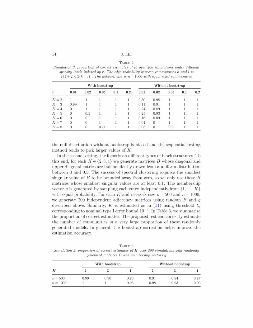
14 J. LEI

Table 2

Simulation 3: proportion of correct estimates of K over 200 simulations under differentsparsity levels indexed by r. The edge probability between communities k and l isr(1 + 2× 1(k = l)). The network size is n= 1000 with equal sized communities

With bootstrap Without bootstrap

r 0.01 0.02 0.05 0.1 0.2 0.01 0.02 0.05 0.1 0.2

K = 2 1 1 1 1 1 0.30 0.98 1 1 1K = 3 0.99 1 1 1 1 0.11 0.91 1 1 1K = 4 0 1 1 1 1 0.24 0.89 1 1 1K = 5 0 0.5 1 1 1 0.25 0.93 1 1 1K = 6 0 0 1 1 1 0.16 0.09 1 1 1K = 7 0 0 1 1 1 0.04 0 1 1 1K = 8 0 0 0.71 1 1 0.03 0 0.9 1 1

the null distribution without bootstrap is biased and the sequential testingmethod tends to pick larger values of K.

In the second setting, the focus is on different types of block structures. Tothis end, for each K ∈ {2,3,4} we generate matrices B whose diagonal andupper diagonal entries are independently drawn from a uniform distributionbetween 0 and 0.5. The success of spectral clustering requires the smallestsingular value of B to be bounded away from zero, so we only use those Bmatrices whose smallest singular values are at least 0.1. The membershipvector g is generated by sampling each entry independently from {1, . . . ,K}with equal probability. For each K and network size n= 500 and n= 1000,we generate 200 independent adjacency matrices using random B and gdescribed above. Similarly, K is estimated as in (11) using threshold tncorresponding to nominal type I error bound 10−4. In Table 3, we summarizethe proportion of correct estimates. The proposed test can correctly estimatethe number of communities in a very large proportion of these randomlygenerated models. In general, the bootstrap correction helps improve theestimation accuracy.

Table 3

Simulation 3: proportion of correct estimates of K over 200 simulations with randomlygenerated matrices B and membership vectors g

With bootstrap Without bootstrap

K 2 3 4 2 3 4

n= 500 0.99 0.90 0.76 0.91 0.84 0.74n= 1000 1 1 0.93 0.98 0.93 0.90

A GOODNESS-OF-FIT TEST FOR STOCHASTIC BLOCK MODELS 15

4.4. The political blog data. The political blog data (Adamic and Glance,2005) records hyperlinks between web blogs shortly before the 2004 US pres-idential election. It has been used widely in the network community detec-tion literature as an example of significant within-community node degreevariation [see Karrer and Newman (2011), Zhao, Levina and Zhu (2012),Jin (2012), e.g.]. It is widely believed that a degree corrected block model ismore suitable for this data, rather than a regular stochastic block model. Yanet al. (2014) used a likelihood ratio method to choose the degree correctedmodel over the regular stochastic block model. Theoretical justification ofthe χ2 approximation used in this method is still an open problem, andmaximizing the likelihood is computationally demanding. Following com-mon practice, we consider the largest connected component of the politicalblog data. There are 1222 nodes with community sizes 586 and 636. We setg to be the true labeling given in the data—the results are similar for g es-timated from the data. Under the null hypothesis that the data is generatedfrom a stochastic block model of two communities, the test statistic is 1172.3for the original test and 491.5 for the bootstrap corrected test, both indi-cating strong evidence to reject the null hypothesis. In addition, we applythe sequential testing procedure at type I error level 10−5, with block modelparameters estimated by spectral clustering using two leading eigenvectorsof the adjacency matrix. The procedure partitions the nodes into 17 groups.Sixteen of these estimated groups mostly contain nodes from one true com-munity, with 8 groups for each community and stratified by degrees. Theadditional estimated group contains nodes with very small degrees, whosecommunity memberships are very hard to recover.

5. Discussion. The goodness-of-fit test developed in this paper is an at-tempt to perform principled statistical inference for stochastic block models.The test statistic reflects a fundamental difference between network modelsand traditional statistical models on independent individuals. In traditionalindependent and identically distributed data samples, the goodness-of-fit isusually assessed by the sum of residuals or squared residuals. For stochasticblock models, the residual is a matrix, where the signal is not carried inthe sum of individual residuals but is determined by how these residualsalign across the rows and columns. For example, suppose A is generatedfrom a stochastic block model with two communities and we want to testif K = 1. If we simply treat the upper diagonal entries of A as indepen-dent Bernoulli variables, the goodness-of-fit test reduces to testing whetherthe n(n− 1)/2 upper diagonal entries look like an independent sample of aBernoulli variable. Such tests have little power in detecting the block struc-ture. On the other hand, the extreme singular value of the residual matrixaccurately captures the block structure. This is an example of detecting low-rank mean effect from a noisy random matrix using its extreme eigenvalues.

16 J. LEI

Other examples using the similar idea include Kargin (2014) for reducedrank multivariate regression and Montanari, Reichman and Zeitouni (2014)for the Gaussian hidden clique problem. It would be interesting to furtherdevelop goodness-of-fit testing methods for more realistic null hypotheses,such as the degree corrected block model or even the nonparametric graphonmodel (Wolfe and Olhede, 2013).

It is possible to extend the method and theory developed in this paperto certain sparse stochastic block models. Consider sparse stochastic blockmodels with B = ρnB0 where the entries of B0 are of order 1 and ρn ↓ 0controls the overall network sparsity. Most random matrix theory used inthis paper (namely, Lemmas A.1, A.3, A.4) has been developed for moder-ately sparse stochastic block models with ρn ≫ n−1/3 in Erdos et al. (2013b,2012). However, existing arguments do not guarantee isotropic delocaliza-tion of eigenvectors (Lemma A.2) due to the heavy tail of the normalizedadjacency matrix entries (Aij−Pij)/[Pij(1−Pij)]. The possibility of provingsuch a result using modified techniques has been mentioned in Erdos et al.(2013a).

APPENDIX: PROOFS

Additional notation. Let (λ∗j , u∗j)nj=1 be the eigenvalue-eigenvector pairs

of A∗ such that λ∗1 ≥ λ∗2 ≥ · · · ≥ λ∗n. For a pair of random sequences (an)

and (bn), we write an = OP (bn) if for any ε > 0 and D > 0 there existsn0 = n0(ε,D) such that

P (an ≥ nεbn)≤ n−D for all n≥ n0.

For any matrix M with singular value decomposition M =∑

j σjujvTj , de-

fine |M | =∑

j |σj |ujvTj . We will use c and C to denote positive constantsindependent of n, which may vary from line to line.

A.1. Results from random matrix theory. We first collect some usefulresults from random matrix theory regarding the distributions of the eigen-values and eigenvectors of A∗.

Lemma A.1 [Asymptotic distributions of λ1(A∗) and λn(A

∗)]. For A∗

defined in (4) we have

n2/3(λ1(A∗)− 2) TW1, n2/3(−λn(A∗)− 2) TW1.

Proof. Let G∗ be an n × n symmetric matrix whose upper diagonalentries are independent normal with mean zero and variance 1/(n− 1), anddiagonal entries are zero. Then A∗ and G∗ have the same first and secondmoments. According to Theorem 2.4 of Erdos, Yau and Yin (2012), we

A GOODNESS-OF-FIT TEST FOR STOCHASTIC BLOCK MODELS 17

know that n2/3(λ1(A∗) − 2) and n2/3(λ1(G

∗) − 2) have the same limitingdistribution. But n2/3(λ1(G

∗)−2) TW1 according to Lee and Yin (2014).The same argument applies to λn(A

∗). �

Lemma A.2 (Eigenvector delocalization). For each deterministic unitvector u and each 1 ≤ j ≤ n, for any ε > 0 and D > 0 there exists n0 =n0(ε,D) such that

P [(uTu∗j)2 ≥ n−1+ε]≤ n−D for all n≥ n0.

It is worth noting that the above result is uniform over j and u in thesense that n0(ε,D) does not depend on u or j. Lemma A.2 can be equiv-

alently stated as (uTu∗j)2 = OP (n

−1) uniformly over all u∗j (1≤ j ≤ n) andall deterministic unit vector u.

Lemma A.2 is Theorem 2.16 of Bloemendal et al. (2014). Although Bloe-mendal et al. (2014) requires the diagonal entries of A∗ to have positivevariance, their Theorem 2.16 is a consequence of the local semicircle law[Theorem 2.12 of Bloemendal et al. (2014)], which can be established formatrices with zero diagonals using the result of Erdos et al. (2013a). Seealso the discussion in Bickel and Sarkar (2013).

Lemma A.3 (Counting large eigenvalues). Let cn be a possibly randomnumber of order oP (1) and m(cn) be the number of eigenvalues of A∗ larger

than λ∗1 − cn. Then m(cn) =OP (nc3/2n ) + OP (1).

Lemma A.3 extends equation (26) of Bickel and Sarkar (2013).

Proof of Lemma A.3. For any a < b < 5, let N∗(a, b) be the num-

ber of eigenvalues of A∗ in the interval (a, b], and N(a, b) = n∫ ba ρsc(x)dx

where ρsc(x) = (1/2π)((4−x2)+)1/2 is the density of the semicircle law. Let

δ(a, b) = N∗(a, b) − N(a, b) then according to Theorem 2.2 of Erdos, Yauand Yin (2012) we have supa,b<5 |δ(a, b)| = OP (1). Then, conditioning onthe event that {|2− λ∗1|+ cn ≤ 1}, we have

m(cn) =N∗(λ∗1 − cn, λ∗1)

=N(λ∗1 − cn, λ∗1) + sup

a,b<5|δ(a, b)|

≤ n

∫ 2

2−(2−λ∗1)−cn

((4− x2)+)1/2 dx+ OP (1)

≤ 2n(cn + |2− λ∗1|)3/2 + OP (1)

≤O(nc3/2n ) + OP (1). �

18 J. LEI

The claimed result follows by observing that the event {|2−λ∗1|+ cn ≤ 1}has probability 1− o(1).

Lemma A.4 (Deviation of largest singular value). There exists absolutepositive constants a, b, c, C, such that

P [n2/3(σ1(A∗)− 2)≥ (logn)a log logn]≤C exp[−b(logn)c log logn].

Lemma A.4 is a direct consequence of equation (2.22) in Erdos, Yau andYin (2012). We can simplify the statement so that there exists an absoluteconstant b > 0 such that for any ε > 0

P [n2/3(σ1(A∗)− 2)≥ nε] =O(n−b).(15)

A.2. Proof of asymptotic null distribution. Now we provide proofs fortheoretical results in Section 3. Here, we omit the dependence on n in g, Band K for simplicity.

Proof of Theorem 3.1. The consistency of g allows us to focus onthe event g = g.

We will prove the claim for λ1(A). The other claim can be proved byapplying the same argument on −A.

Let A′ ∈Rn×n be such that

A′ij =

Aij − Pij√

(n− 1)Pij(1− Pij), i 6= j,

Pii − Pii√

(n− 1)Pii(1−Pii), i= j.

(16)

Thus, A′ = A∗ +∆′, where ∆′ij = (Pij − Pij)/

√

(n− 1)Pij(1−Pij). Because

∆′ is a K×K block-wise constant symmetric matrix, its rank is at most K,and the corresponding principal subspace is spanned by (θ1, . . . , θK), whereθk ∈R

n is the unit norm indicator of the kth community in g. That is, the

ith entry of θk is n−1/2k if gi = k and zero otherwise, where nk is the size of

the kth community.The consistency of g implies that with probability tending to one, for

each 1≤ k, k′ ≤K, Bk,k′ is the sample mean of independent Bernoulli ran-dom variables with parameter Bk,k′ and sample size of order (n/K)2. Thus,standard large deviation inequalities such as Bernstein’s inequality or Ho-effding’s inequality suggest that supk,k′ |Bk,k′−Bk,k′|= oP (K logn/n), which

implies that supi,j |Pij − Pij| = oP (K logn/n). Note here the oP statement

goes through a union bound over K2 terms, which is valid since the tailprobability bound for Pij − Pij can be made exponentially small in n. Let

A GOODNESS-OF-FIT TEST FOR STOCHASTIC BLOCK MODELS 19

∆′ = ΘΓΘT , where Θ = (θ1, . . . , θK) and Γ is a K ×K symmetric matrix.Then each entry of Γ is oP (n

−1/2 logn), and hence ‖Γ‖= oP (Kn−1/2 logn).

We will show that

λ1(A′) = λ1(A

∗) + oP (n−2/3),(17)

by establishing a lower and upper bound on λ1(A′). Both parts uses the

eigenvector delocalization result (Lemma A.2) as follows. Let Θ = (θ1, . . . , θK),then, uniformly over j we have

‖ΘTu∗j‖22 =K∑

k=1

(θTk u∗j )

2 = OP (Kn−1),(18)

and hence

|(u∗j)T∆′u∗j | ≤ |(ΘTu∗j )TΓ(ΘTu∗j )| ≤ ‖ΘTu∗j‖22‖Γ‖

(19)= OP (K

2n−3/2 logn).

Here, the OP statement in (18) holds when taking union bound over Kterms by choosing D large enough in Lemma A.2.

First, we provide a lower bound on λ1(A′):

λ1(A′)≥ (u∗1)

T A′u∗1 = λ∗1 + (u∗1)T∆′u∗1

≥ λ∗1 − OP (K2n−3/2 logn)(20)

≥ λ∗1 − oP (n−2/3),

where the last inequality uses the assumed upper bound on the rate at whichK grows with n, and the second last inequality uses (19).

Next, we provide an upper bound of λ1(A′). For any unit vector u ∈R

n,let (a1, . . . , an) be a unit vector in R

n such that

u=

n∑

j=1

aju∗j .

Let m be the number of λ∗j ’s in the interval (λ∗1 − 2‖∆′‖, λ∗1], and u1 =∑m

j=1 aju∗j , u2 =

∑nj=m+1 aju

∗j . Then

uT A′u= uT A∗u+ uT∆′u

≤ λ∗1

m∑

j=1

a2j + (λ∗1 − 2‖∆′‖)n∑

j=m+1

a2j + 2uT1 |∆′|u1 +2uT2 |∆′|u2

≤ λ∗1

m∑

j=1

a2j + (λ∗1 − 2‖∆′‖)n∑

j=m+1

a2j

20 J. LEI

+ 2m

m∑

j=1

a2j(u∗j )T |∆′|u∗j +2uT2 |∆′|u2

≤ λ∗1

m∑

j=1

a2j + (λ∗1 − 2‖∆′‖)n∑

j=m+1

a2j(21)

+ 2mOP (K2n−3/2 logn)

m∑

j=1

a2j + 2‖∆′‖n∑

j=m+1

a2j

≤ λ∗1 +mOP (K2n−3/2 logn)

≤ λ∗1 + (O(n‖∆′‖3/2) + OP (1))OP (K2n−3/2 logn)

= λ∗1 + OP (K7/2(logn)5/2n−5/4),

where the third inequality uses (19) and uniformity over j, and the second

last line uses Lemma A.3 together with ‖∆′‖= oP (Kn−1/2 logn).

Thus, (17) is established by combining (20) and (21), provided that K =O(n1/6−τ ) for some small positive τ .

Next, we show that λ1(A) = λ1(A′) + oP (n

−2/3). Let A′′ = A′ − diag(A′).

Consider the block representation of A:

A= (A(k,l))Kk,l=1,

where A(k,l) is the submatrix corresponding to the rows in community k andcolumns in community l. Similar block representations can be defined forA′′. It is obvious that

A(k,l) = A′′(k,l)

√

Bkl(1−Bkl)√

Bkl(1− Bkl)= A′′

(k,l)(1 + oP (Kn−1 logn)).

Therefore,

‖A− A′′‖ ≤Kmaxk,l

‖A(k,l) − A′′(k,l)‖ ≤ oP (Kn

−1 logn)K∑

k,l

‖A′′(k,l)‖

≤ oP (K2n−1 logn)‖A′′‖ ≤ oP (K

2n−1 logn)(‖A′‖+ ‖diag(A′)‖)≤ oP (K

2n−1 logn)(OP (1) +OP (Kn−3/2 logn))

= oP (K2n−1 logn) = oP (n

−2/3).

Then

‖A− A′‖ ≤ ‖A− A′′‖+ ‖diag(A′)‖= oP (n−2/3).(22)

Combining (17) and (22), we have

λ1(A) = λ1(A∗) + oP (n

−2/3).(23)

A GOODNESS-OF-FIT TEST FOR STOCHASTIC BLOCK MODELS 21

Now applying Lemma A.1 and combining with (23) we have

n2/3(λ1(A)− 2) TW1. �

A.3. Proof of power and consistency.

Proof of Theorem 3.3. For all 1 ≤ l ≤K, 1 ≤ k ≤K0, let Nl = {i :gi = l}, Nk = {i : gi = k} and Nk,l = {i : gi = k, gi = l}. For each 1 ≤ l ≤K,

Nl is partitioned into {Nk,l : 1 ≤ k ≤K0}. Thus, for each 1 ≤ l ≤ K there

exists a kl such that 1 ≤ kl ≤K0 and |Nkl,l| ≥ |Nl|/K0 ≥ c0n/(K ×K0) ≥c0nK

−2. Because K0 <K, there exist l1 and l2 such that kl1 = kl2 = k. SinceB ∈ BK , there exists an l3 such that Bl1,l3 6=Bl2,l3 . Let k

′ = kl3 and we have

|Nk′,l3 | ≥ c0nK−2.

Let A(0) be the submatrix of A consisting the rows in Nk,l1 ∪ Nk,l2 , and

the columns in Nk′,l3 . Define A(0), P (0), and P (0) correspondingly.

When k 6= k′, or k = k′ but l3 /∈ {l1, l2}, the submatrix A(0) contains only

off-diagonal entries of A. Therefore, P (0) is a constant matrix in that all ofits entries are equal. We have

‖A‖ ≥ ‖A(0)‖ ≥ n−1/2‖A(0) − P (0)‖≥ n−1/2(‖P (0) − P (0)‖ − ‖A(0) − P (0)‖)

(24)≥ n−1/2(‖P (0) − P (0)‖ −OP (n

1/2))

≥ n−1/2(δBc0nK−2/2−OP (n

1/2)).

To obtain the last inequality, first note that P (0) has two distinct blockseach with at least c0nK

−2 rows and at least c0nK−2 columns. Each of these

two blocks has constant entries and at least one of them has absolute entryvalue at least δB/2. Thus, ‖P (0) − P (0)‖ ≥ δBc0nK

−2/2.When k = k′ and l3 ∈ {l1, l2}, the submatrix A(0) defined above contains

diagonal entries of A. The corresponding entries of P (0) are zero. These zero

entries causes an additional O(1) term in ‖P (0) − P (0)‖ and (24) still goesthrough. �

Proof of Corollary 3.4. Following the notation in the proof ofTheorem 3.3, for any K0 < K we have, in view of (24) and letting C =infn δBc0/2,

P (Tn,K0 < tn) = P [n2/3(‖A‖ − 2)< tn] = P [‖A‖<n−2/3tn + 2]

≤ P [n−1/2(‖P (0) − P (0)‖ − ‖A(0) −P (0)‖)≤ n−2/3tn +2]

≤ P [n−1/2‖A(0) −P (0)‖ ≥Cn1/2K−2 − n−2/3tn − 2]

≤ n−1,

22 J. LEI

the last inequality is obtained by first using the assumption K =O(n1/6−τ ),

and tn =O(n5/6), so that Cn1/2K−2 + n−2/3tn + 2≥ n1/6 for large n, andthen applying operator norm deviation bound results such as Theorem 5.2of Lei and Rinaldo (2013) [see also Theorem 3.4 of Chatterjee (2015)].

Therefore,

P (K <K)≤K−1∑

K0=1

P (Tn,K0 < tn)≤ n−1(K − 1) = o(1).

On the other hand,

P (K >K)≤ P (Tn,K ≥ tn) = P (n2/3(σ1(A)− 2)≥ tn)

≤ P (n2/3(σ1(A∗)− 2)≥ tn/2) + P (n2/3|σ1(A∗)− σ1(A)| ≥ tn/2)

= o(1),

where the first probability is controlled using Lemma A.4 and the secondprobability is controlled using (23) and its analogous result for λn(A) −λn(A

∗). �

A.4. Asymptotic power against degree corrected block models.

Proof of Theorem 3.5. Recall that Nl,k = {i : gi = k, gi = l} (1≤ l≤K0, 1≤ k ≤K). Let φk,Nl,k

be the subvector of φk on the entries in Nl,k.

Let ηl = φk∗,Nl,k∗for each 1≤ l ≤K0. By definition of E , ∑K0

l=1 E(ηl,1)≥E(ψk∗ ,K0), and hence there exists an l∗ such that E(ηl∗ ,1)≥ E(φk∗ ,K0)/K0.

For simplicity, denote η = ηl∗ and η = η/‖η‖. Let m= |Nl∗,k∗| and defineem as the 1×m vector with 1/

√m on each entry. Therefore, we have

‖η − em‖2 ≥ E(η,1) = ‖η‖−2E(η,1)≥ ‖η‖−2E(φk∗ ,K0)/K0.(25)

Because η and em both have unit ℓ2 norm, (25) implies that

|eTmη| ≤ 1− E(φk∗ ,K0)

2K0‖η‖2.

Let u= (η− emeTmη)/‖η − eme

Tmη‖, then

uT η = uT η‖η‖= ‖η‖ 1− (eTmη)2

‖η − emeTmη‖

≥ E(φk∗ ,K0)

2K0‖η‖≥ E(φk∗ ,K0)

2K0.(26)

Now let k′ be such that Bk∗,k′ = ‖Bk∗,·‖∞. There exists an l′ such that

‖φk′,Nl′,k′‖ ≥K

−1/20 .

A GOODNESS-OF-FIT TEST FOR STOCHASTIC BLOCK MODELS 23

Let A(0) be the submatrix of A corresponding to the rows in Nl∗,k∗ and

columns in Nl′,k′ , and define A(0), P (0), P (0) similarly. Thus, by construction

we have, letting m′ = |Nl′,k′ |,

P (0) = ‖φk∗‖‖φk′‖Bk∗k′ηφTk′,Nl′,k′, P (0) = Bl∗l′

√mm′eme

Tm′ .

Observing that uTem = 0, we have

‖uT (P (0) − P (0))‖= ‖uTP (0)‖= ‖ψk∗‖‖ψk′‖Bk∗k′ |uT η|‖φk′,Nk′,l′‖

≥ ‖ψk∗‖‖ψk′‖Bk∗k′E(φk∗ ,K0)

2K3/20

≥ κnn‖Bk∗,·‖∞E(φk∗ ,K0)

2K3/20

.

The claimed result follows by observing that

‖A(0)‖ ≥ n−1/2(‖P (0) − P (0)‖ − ‖A(0) −P (0)‖)and ‖A(0) −P (0)‖=OP (

√n). �

REFERENCES

Abbe, E., Bandeira, A. S. and Hall, G. (2014). Exact recovery in the stochastic blockmodel. Preprint. Available at arXiv:1405.3267.

Adamic, L. A. and Glance, N. (2005). The political blogosphere and the 2004 USelection: Divided they blog. In Proceedings of the 3rd International Workshop on LinkDiscovery 36–43. ACM, New York.

Airoldi, E. M., Blei, D. M., Fienberg, S. E. and Xing, E. P. (2008). Mixed mem-bership stochastic blockmodels. J. Mach. Learn. Res. 9 1981–2014.

Amini, A. A. and Levina, E. (2014). On semidefinite relaxations for the block model.Preprint. Available at arXiv:1406.5647.

Anandkumar, A., Ge, R., Hsu, D. and Kakade, S. M. (2014). A tensor approach tolearning mixed membership community models. J. Mach. Learn. Res. 15 2239–2312.MR3231594

Bickel, P. J. and Chen, A. (2009). A nonparametric view of network models andNewman–Girvan and other modularities. Proc. Natl. Acad. Sci. USA 106 21068–21073.

Bickel, P. J. and Sarkar, P. (2013). Hypothesis testing for automated communitydetection in networks. Preprint. Available at arXiv:1311.2694.

Bloemendal, A., Erdos, L., Knowles, A., Yau, H.-T. and Yin, J. (2014). Isotropiclocal laws for sample covariance and generalized Wigner matrices. Electron. J. Probab.19 1–53. MR3183577

Chatterjee, S. (2015). Matrix estimation by universal singular value thresholding. Ann.Statist. 43 177–214. MR3285604

Chaudhuri, K., Chung, F. and Tsiatas, A. (2012). Spectral clustering of graphs withgeneral degrees in the extended planted partition model. J. Mach. Learn. Res. WorkshopConf. Proc. 2012 35.1–35.23.

24 J. LEI

Chen, K. and Lei, J. (2014). Network cross-validation for determining the number ofcommunities in network data. Preprint. Available at arXiv:1411.1715.

Chen, Y., Sanghavi, S. and Xu, H. (2012). Clustering sparse graphs. In Advances inNeural Information Processing Systems 25 (F. Pereira, C. J. C. Burges, L. Bottou

and K. Q. Weinberger, eds.) 2204–2212. Curran Associates, Red Hook, NY.Decelle, A., Krzakala, F., Moore, C. and Zdeborova, L. (2011). Asymptotic analy-

sis of the stochastic block model for modular networks and its algorithmic applications.Phys. Rev. E (3) 84 066106.

Erdos, L., Yau, H.-T. and Yin, J. (2012). Rigidity of eigenvalues of generalized Wignermatrices. Adv. Math. 229 1435–1515. MR2871147

Erdos, L., Knowles, A., Yau, H.-T. and Yin, J. (2012). Spectral statistics of Erdos-Renyi Graphs II: Eigenvalue spacing and the extreme eigenvalues. Comm. Math. Phys.314 587–640. MR2964770

Erdos, L., Knowles, A., Yau, H.-T. and Yin, J. (2013a). The local semicircle law fora general class of random matrices. Electron. J. Probab. 18 no. 59, 58. MR3068390

Erdos, L., Knowles, A., Yau, H.-T. and Yin, J. (2013b). Spectral statistics of Erdos–Renyi graphs I: Local semicircle law. Ann. Probab. 41 2279–2375. MR3098073

Fishkind, D. E., Sussman, D. L., Tang, M., Vogelstein, J. T. and Priebe, C. E.

(2013). Consistent adjacency-spectral partitioning for the stochastic block model whenthe model parameters are unknown. SIAM J. Matrix Anal. Appl. 34 23–39. MR3032990

Holland, P. W., Laskey, K. B. and Leinhardt, S. (1983). Stochastic blockmodels:First steps. Soc. Netw. 5 109–137. MR0718088

Jin, J. (2012). Fast community detection by SCORE. Available at arXiv:1211.5803.Kargin, V. (2014). On the singular values of the reduced-rank multivariate response

regression. Preprint. Available at arXiv:1409.6779.Karrer, B. and Newman, M. E. J. (2011). Stochastic blockmodels and community

structure in networks. Phys. Rev. E (3) 83 016107, 10. MR2788206Krzakala, F., Moore, C., Mossel, E., Neeman, J., Sly, A., Zdeborova, L. and

Zhang, P. (2013). Spectral redemption in clustering sparse networks. Proc. Natl. Acad.Sci. USA 110 20935–20940. MR3174850

Lee, J. O. and Yin, J. (2014). A necessary and sufficient condition for edge universalityof Wigner matrices. Duke Math. J. 163 117–173. MR3161313

Lei, J. and Rinaldo, A. (2013). Consistency of spectral clustering in stochastic blockmodels. Preprint. Available at arXiv:1312.2050.

Lei, J. and Zhu, L. (2014). A generic sample splitting approach for refined communityrecovery in stochastic block models. Preprint. Available at arXiv:1411.1469.

Massoulie, L. (2013). Community detection thresholds and the weak Ramanujan prop-erty. Preprint. Available at arXiv:1311.3085.

McSherry, F. (2001). Spectral partitioning of random graphs. In 42nd IEEE Symposiumon Foundations of Computer Science (Las Vegas, NV, 2001) 529–537. IEEE ComputerSoc., Los Alamitos, CA. MR1948742

Montanari, A., Reichman, D. and Zeitouni, O. (2014). On the limitation of spec-tral methods: From the Gaussian hidden clique problem to rank one perturbations ofGaussian tensors. Preprint. Available at arXiv:1411.6149.

Mossel, E., Neeman, J. and Sly, A. (2013). A proof of the block model thresholdconjecture. Preprint. Available at arXiv:1311.4115.

Newman, M. E. (2006). Modularity and community structure in networks. Proc. Natl.Acad. Sci. USA 103 8577–8582.

Newman, M. E. and Girvan, M. (2004). Finding and evaluating community structurein networks. Phys. Rev. E (3) 69 026113.

A GOODNESS-OF-FIT TEST FOR STOCHASTIC BLOCK MODELS 25

Saldana, D. F.,Yi, Y. and Feng, Y. (2014). How many communities are there? Preprint.Available at arXiv:1412.1684.

Vu, V. (2014). A simple SVD algorithm for finding hidden partitions. Preprint. Availableat arXiv:1404.3918.

Wolfe, P. J. and Olhede, S. C. (2013). Nonparametric graphon estimation. Preprint.Available at arXiv:1309.5936.

Yan, X., Shalizi, C., Jensen, J. E., Krzakala, F., Moore, C., Zdeborova, L.,Zhang, P. and Zhu, Y. (2014). Model selection for degree-corrected block models. J.Stat. Mech. Theory Exp. 2014 P05007.

Zhao, Y., Levina, E. and Zhu, J. (2011). Community extraction for social networks.Proc. Natl. Acad. Sci. USA 108 7321–7326.

Zhao, Y., Levina, E. and Zhu, J. (2012). Consistency of community detection in net-works under degree-corrected stochastic block models. Ann. Statist. 40 2266–2292.MR3059083

Department of Statistics

Carnegie Mellon University

Pittsburgh, Pennsylvania 15213

USA

E-mail: jinglei@andrew.cmu.edu