-::^^^*^7":-;s;::>:- ■ MliniCPPmq|!niIBWVIH«MaH!!llPWIIMIlli'UUi<IWUlW!UIW,,.

N

<

3 BRANCH AND BOUND METHODS

FOR THE TRAVELING SALESMAN PROBLEM

by

Egon Balas Carnegie-Mellon University

and

Paolo Toth University of Florence

Carnegie-Mel Ion University PITTSBURGH, PENNSYLVANIA 15213

GRADUATE SCHOOL OF INDUSTRIAL ADMINISTRATION WIUIAM LARIMER MELLON, FOUNDER

V

o M-»•'■■ / if K 2 -r:: *m 01983" «1

A

t i'his (ionj;if;;)j he: br-an aprsiüved ! fr.x P.::fcii.-: s- '-':; • ^"'-; "^c; its

QQ fU OJL ^gQ

pB>!Bt^iptp«giigglcisagi»gPW»'^^

W.P.#45-82-83

Management Science Research Report No. MSRR 488

BRANCH AND BOUND METHODS

FOR THE TRAVELING SALESMAN PROBLEM

by

Egon Balas Carnegie-Mellon University

and

Paolo Toth University of Florence

March 1983

h . a 2 0 1983. ■: j|f

The research of the first author was supported by Grant ECS-8205425 of the National Science Foundation and Contract N00014-75-C-0621 NR 047-048 with the U.S. Office of Naval Research; and that of the second author by the Centro Nazionale delle Ricerche of Italy.

Management Science Research Group Graduate School of Industrial Administration

Carnegie-Mellon University Pittsburgh, Pennsylvania 15213

-h

S5SHpspHBpp^BP3!iPiP8P'"*<? jPl'SJlLli-,,.! 4J,,J-,!iWI,if W,.J,»J

ABSTRACT

This paper reviews the state of the art in enumerative solution methods

for tu. traveling salesman problem (TSP). The introduction (Section 1)

discusses the main ingredients of branch and bound methods for the TSP.

Sections 2, 3 and 4 discuss classes of methods based on three different re-

laxations of the TSP: the assignment problem with the TSP cost function, the

1-tree problem with a Lagrangean objective function, and the assignment

problem with a Lagrangean objective function. Section 5 briefly reviews some

other relaxations of the TSP, while Section 6 discusses the performance of

some state of the art computer codes. Besides material from the literature,

the paper also includes the results and statistical analysis of some computa-

tional experiments designed for the purposes of this review.

Codes

Special

V

^wB§|§agiHpp^is^^^ -—— _ — ——■■^r^.—- ! ■ —

BRANCH AND BOUND METHODS

FOR THE TRAVELING SALESMAN PROBLEM

by

Egon Balas and Paolo Toth

1. Introduction 1

Branch and bound method for the TSP 4

Version 1 4

Version 2 , 5

2. Relaxation I: The Assignment Problem with the TSP Cost Function 7

Branching rules. ........ ..... 9 Other features ...................14

3. Relaxation II: The 1-Tree Problem with Lagrangean Objective Function . ....15

Branching rules. , 22

Other features ... .........24

Extension to the asymmetric TSP 24

4. Relaxation III: The Assignment Problem with Lagrangean Objective Function 25

Bounding procedure 1..... 29

Bounding procedure 2.. 33

Bounding procedure 3.. 3g

Additional bounding procedures 41

Branching rules and other features 43

5. Other Relaxations. .............,...45

The 2-matching relaxation 46

The n-path relaxation. .... 47

The LP with cutting planes as a relaxation 48

6. Performance of State of the Art Computer Codes . . , 48

The asymmetric TSP 48

The symmetric TSP ..... 52

Average performance as a function of problem size. . 54

EXERCISES 60

REFERENCES 63

■ Tl, ...,,. .

1. Introduction

Since the first attempt to solve traveling salesman problems by an enumer-

atlve approach, apparently due to Eastman [1958], many such procedures have been

proposed. In a sense the TSP has served as a testing ground for the development

of solution methods for discrete optimization, in that many procedures and,devices

were first developed for the TSP and then, after successful testing, extended to -vj

more general Integer programs. The term "branch and bound" itself was coined by

Little, Murty, Sweeney and Karel [1963] in conjunction with their TSP algorithm.

Enumerative (branch and bound, implicit enumeration) methods solve a dis-

crete optimization problem by breaking up its feasible set into successively

smaller subsets, calculating bounds on the objective function value over each

subset, and using them to discard certain subsets from further consideration.

The bounds are obtained by replacing the problem over a given subset with an easier

(relaxed) problem, such that the solution value of the latter bounds that of the

former. The procedure ends when each subset has either produced a feasible

solution, or was shown to contain no better solution than the one already in

hand. The best solution found during the procedure is a global optimum.

For any problem P, we denote by v(P) the value of (an optimal solution

to) P. The essential ingredients of any branch and bound procedure for a dis-

crete optimization problem P of the form minf.f(x)|x € S-} are

(i) a relaxation of P, i.e. a problem R of the form min''g(x)|x t T},

such that SST and for every x,y€S, f(x) < f(y) implies g(x) < g(y).

(11) a branching or separation rule, I.e. a rule for breaking up the

feasible set S, of the current subproblem P. into subsets

q S<,,..., S , such that J S..-S.; 11 iq i«i lJ l

mmw-nrr-^rm jHigtjyffimiü li^WB^^-l"^-"1^!^^**'^11,1 - - - - ' ■*.-... - .- -.iMTOywjBpw

(iii) a lower bounding procedure, i.e. a procedure for finding (or

approximating from below) v(R.) for the relaxation R. of each

subproblem P ; and

(iv) a subproblem selection rule, i.e. a rule for choosing the next

subproblem to be processed.

Additional ingredients, not always present but always useful when present,

are

(v) an upper bounding procedure, i.e. a heuristic for finding feasible

solutions to P; and

(vi) a testing procedure, i.e., a procedure for using the logical implications

of the constraints and bounds to fix the values of some variables

(reduction, variable fixing) or to discard an entire subproblem

(dominance tests).

For more information on enumerative methods in integer programming see,

for instance, Chapter 4 of Garfinkel and Nemhauser [1972], and/or the surveys

by Balas [1975], Balas and Guignard [1979], Beale [1979], Speilberg [1979].

Since by far the most important ingredient is (i), we will classify the

branch and bound procedures for the TSP according to the relaxation that they

use.

The integer programming formulation of the TSP that we will refer to when

discussing the various solution methods is defined on a complete directed graph

G - (V,A) on n nodes, with node set V - [I n}, arc set A • {(i,J)|l,J - l,...,n},

and nonnegative costs c associated with the arcs. The fact that G is

mmm^jmrnim^ammmi'. —

flfn^ntia^ESnBBBHB ^-™^^™^^^v^^^j^ —».^»TWWWI'-J^" ■«-■inLii i i.nyT'.'i' | 'JW» " '■' gjm ' g! *?!TS^

complete involves no restriction, since arcs that one wishes to ignore can be

assigned the cost c.. » ». In all cases c.. » », V i€v. The TSP can be

formulated, following Dantzig, Fulkerson and Johnson [1954], as the problem

(1) min 2 2 c x i€Vj€V iJ 1J

i; s.t.

(2)

2 x. - 1 , i€V

2 x - 1 , j€V i€V 1J

(3)

(4)

iSSjcS '*, < Is!-1 .

x « 0 or 1, i,j€V.

V S c V, S«

where x - 1 if arc (i,j) is in the solution, x^ - 0 otherwise.

The subtour elimination inequalities (3) can also be written as

(5) 2 2 x > 1 , i€Sj€V\S 1J

V S CJ V, Sji0

A very important special case is the symmetric TSP, in which c^. ■ c.^

Vi,j . The symmetric TSP can be defined on a complete undirected graph G -(V,E)

on n nodes, with node set V, edge set E, and arbitrary costs c... It can

be stated as

(6)

s.t.

(7)

min ». <- c, ,x i€Vj>i 1J lj

•> X . , + i. X, , »2 , j<i Ji j>i lj

i€V

,,,,aigr<*Tr'T"'iiiif5lT*E^^Ba!Bt°g,Bg"

(8) S Z>: < |S -I, V SC V, Stf l£Sj€S 1J *

J>i

(9) xlj - 0 or 1, i,j€V , j>i

where the subtour elimination inequalities (8) can also be written as

(10) Z S x,. + 2 Zx..>2, V S C V, sm i€Sj€v\S 1J i€V\Sj€S 1J

j>i j>i

Next we outline two versions of a branch and bound procedure for the TSP.

prior to using any of these versions, a relaxation R of the TSP must be

chosen. Both versions carry at all times a list of active subproblems. They

differ in that version 1 solves a (relaxed) subproblem R. only when node k is

selected and taken off the list, while version 2 solves each (relaxed) sub-

problem as soon as it is created, i.e. before it is placed on the list.

Although the branch and bound procedures used in practice differ among them-

selves in many details, nevertheless all of them can be viewed as variants of

one of these two versions.

Branch and bound method for the TSP

Version 1

1. (initialization), put TSP on the list (of active subproblems). Initia-

lize the upper bound at U ■ «, and go to 2.

2. (Subproblem selection). If the list is empty, stop: the tour associated

with Ü is optimal (orj if u « ., TSP ha8 no solution). Otherwise choose

a subproblem TSPj^ according to the subproblem selection rule, remove TSP,

from the list, and go to 3.

Txrnrpiiiiiiitiii'iiiiri'^''" fg^gWPSWg^iJBMSa^ifaiiag

3. (Lower bounding). Solve the relaxation R of TSP or bound v(R ) from

below, and let L, be the value obtained.

If L, > U, return to 2.

If L. < U and the solution defines a tour for TSP, store it in place

of the previous best tour, set U - L,, and go to 5.

If L. < U and the solution does not define a tour, go Co 4.

4. (Upper bounding: optional). Use a heuristic to find a tour in TSP. If

a better tour is found than the current best, store it in place of the

latter and update U. Go to 5.

5. (Reduction: optional). Remove from the graph of TSP all the arcs whose

inclusion in a tour would raise its value above U, and go to 6.

5. (Branching). Apply the branching rule to TSP., i.e. generate new

subproblems TSP..,..., TSP , place them on the list, and go to 2.

Version 2

1. (Initialization). Like in version 1, but solve R before putting TSP

on the list.

2. (Subproblem selection). Same as in version 1.

3. (Upper bounding: optional). Same as step 4 of version 1, with "go to 5"

replaced by "go to 4."

4. (Reduction: optional). Same as step 5 of version 1, with "go to 6" replaced

by "to go 5."

5. (Branching). Use the branching rule to define the set of subproblems

TSP..,.,.,TSP to be generated from the current subproblem TSP.,

and go to 6.

.!"■■ ii'WJUWHU.lJUMIi'iP" ■w'"l'ii"~w.n'-".~ - """"'"; " ' 'Wi»W^iWW

6. (Lower bounding). If all the sufaproblems to be generated from TSP

according to the branching rule have already been generated, go to 2.

Otherwise generate the next subproblem TSP., defined by the branching

rule, solve the relaxation R of TSP or bound v(R ) from below, ij tj ij

and let L.. be the value obtained.

If L.. > U, return to 6.

If L., < U and the solution defines a tour for TSP, stora it in place

of the previous best tour, set U - L. ., and go to 6.

If L. < Ü and the solution does not define a tour, place TSP on the list

and return to 6.

In both versions, the procedure can be represented by a rooted tree (search

or branch and bound tree) whose nodes correspond to the subproblems generated,

with the root node corresponding to the original problem, and the successor nodes

of a given node i associated with TSP. corresponding to the subproblems

TSP,.,...,TSP. defined by the branching rule.

It is easy to see that under very mild assumptions on the branching rule

and the relaxation used, both versions of the above procedure are finite (see

Exercise 1).

Next we discuss various specializations of the procedure outlined above,

classified according to the relaxation that they use. When assessing and

comparing the various relaxations, one should keep in mind that a "good" re-

laxation is one that (i) gives a strong lower bound, i.e. yields a small

difference v(TSP) - v(R) ; and (ii) is easy to solve. Naturally, these are

often conflicting goals, and in such cases one has to weigh the tradeoffs.

:i

■ÜPH^SWK

2. Relaxation I: The Assignment Problem with the TSP Cost Fuucticn

The most straightforward relaxation of the TSP, and historically the first

one to have been used, is the problem obtained from the integer programming

formulation (1), (2), (3), (4) by removing the constraints (3), i.e. the

assignment problem (AP) with the same cost function as TSP. It was used,

among others, by Eastman [1958], Little, Murty, Sweeney and Karel [1963],

Shapiro [1966], Bellmore and Malone [1971], Smith, Srinivasan and Thompson

[1977], Carpaneto and Toth [1980].

An assignment (i.e., a solution to AP) is a union of directed cycles,

hence either a tour, or a collection of subtours. There are nl distinct

assignments, of which (n-1)! are tours. Thus on the average one in every n

assignments is a tour. Furthermore, in the current context only those assign-

ments are of interest that contain no diagonal elements (i.e., satisfy x *

0, i«l,**«,n), and their number is n!/e rounded to the nearest integer,

i.e. ln!/e + 1/2] (see, for example, Hall [1967], p. 10). Thus on the average one

in every n/e "diagonal-free" assignments is a tour. This relatively high fre-

quency of tours among assignments suggests that v(AP) is likely to be a pretty

strong bound on v(TSP), and computational experience with AP-based solution

methods supports such a view. To test how good this bound actually is for

randomly generated problems, we performed the following experiment. We gen-

erated 400 problems with 50 < n < 250 with the costs independently drawn from a

uniform distribution of the integers over the intervals [1,100] and [1,1000],

and solved both AP and TSP. We found that on the average v(AP) was 99.27. of

v(TSP), furthermore, we found the bound to improve with problem size, in that

for the problems with 50 < n < 150 and 150 < n < 250 the outcomes were 98.8%

and 99.5%, respectively.

s»^^s^F»~^'>w™w«j»w|ipjip!4pp!ism i ST»' - •• - -.-—• --T——T . •^|lH|m^llmtKMwflßmW^'^K^'~■* ' !«™n'?SW>™sKTs™E»,,'^Taj

, j v„ <** Hungarian method (Kuhn [1955]; for a more recent AP can b« solved by the nun«

..... ri9751 or Lawler Q9761 > in at most 0(n ) steps. .»mmnt see Christofides IJ.*'-M

treatment, solved at every node of the search tree differ The assignment problems AJ?t w

.,__int oroblem AP in »at some arcs are excluded «'forbidden) from the initial assignment pro

a .f. included (force» into the solution. These modifi- from, while other arcs are mciu

-♦. «nv difficulty. S^e the Hungarian method provides at cations do not present any m*

, i««»r bound onv(AP), C process of solving a subproblem can every iteration a lower o«

«». fh* lower bound meetfhe upper bound U. More importantly, be stopped whenever tn«=

r«» the branching rä below), the assignment problem AP in the typical case <.see j

, t e t-he search treiffers from the problem AP. solved to be solved at node j of tne i

i -.1« in that a c»in arc belonging to the optimal solution at the parent node i only

o£ AP is excluded from the solution of, and possibly some other arcs are

1 J ,-v,- same position or out) with respect to the solution required to maintain the san v

that they have with respect to of AP^ Whenever this is the case,

be solved by the Hiian method starting from the optimal the problem AP^ can

blem at the parent nor at a brother node), in at most 0(n )

... i ar Bellmore and fc [ 1971]). For an efficient implementa- steps (see Exercise i or

ersion of the Hungariaiod, which uses on the average consider-

n,J\ steps, see Carpand Toth [1980]. The primal simplex ably less than 0(n ) «*P »

for the assignment problem has sen used in a parametric version

tlv this sequence of slated assignment problems by

It,., HUM—> - *"**"» lW771, A »(XP'i can be slimproved by addition of a penalty.

The lower bound v^r;

. d a8 the minimal e in the objective function This can be calculate

first simplex pivottiminates some arc from the caused ei-her by

. et~qt iteration of Urian method that accomplishes the same solution, or by a EIS

Furthermore, the arc to be inc the solution by the pivot can be

-■■■-rrrim J.:i'-fii

restricted to a cutset defined by some subtour of the AF solution. Computa-

tional experience indicates, however, that the impact of such a penalty tends

to decrease with problem size and is negligible for anything but small problems.

In the computational experiment involving the 400 randomly generated problems

that we ran, the addition of a penalty to v(AP) raised the value of the lower

bound on th« average by 0.03%, from 99.27. to 99.237. of v(TSP).

Branching rules

Several branching rules have been used in conjunction with the AP relax-

ation of the ISP. In assessing the advantages and disadvantages of these rules

one should keep in mind that the ultimate goal is to solve the ISP by solving

as few subproblems as possible. Thus a "good" branching rule is one that

(a) generates few successors of a node of the search tree, and (b) generates

strongly constrained subproblems, i.e. excludes many solutions from each

subproblem. Again, these criteria are usually conflicting and the merits of

the various rules depend on the tradeoffs.

We will discuss the various branching rules in terms of sets of arcs

excluded (E.) from, and included (1^) into the solution of subproblem

k. In terms of the variables x ., the interpretation of these sets is that

subproblem k is defined by the conditions

/

(11) ij

0, (i,j) € E. x,, « <

1, (i,j) € ^

in addition to (1), (2), (3), (4). Thus the relaxation of subproblem k is

given by (11) in addition to (1), (2), (4). We abbreviate Branching Rule

by 3R.

gggaBgjjg#iWi|g*»W^-*)''-*-'-'*'--'--. aPfJWiapWjIBBPIBlPpwy ' ■-»ME»»W» ip^|Bpp^p||||p|pj!^B|^|p|jppjpi

10

BR lt (Little, Murty, Sweeney and Karel [1963]). Given the current re-

laxed subproblem AP. and its reduced costs c.. - c.. - u. - v., where u. it ij lj 1 j i

and v. are optimal dual variables, for every arc (i,J) such that c.. « 0

define the penalty

p - min [clh : h€V\{ j]} + min {c : h€V\fi}]-

and choose (r,s) € A such that

Prs " °" {Pij ! 'ij ' °} •

Then generate two successors of node k, nodes k + 1 and k + 2, by

defining

and M-HUCCr..» , \+1'\

h*2mh> Ifcrt-lfcUCCr..)] •

This rule does not use the special structure of the TSP (indeed, it applies

to any integer program), and has the disadvantage that it leaves the

optimal solution to AP feasible for AP..

The following rules are based on disjunctions derived from the subtour

elimination inequalities (3) or (5),

BR 2. (Eastman [1958], Shapiro [1966]). Let x be the optimal solution to

the current relaxed subproblem AP, and let A- • {(i.,i,),...,(it,i,)J be the

arc set of a minimum cardinality subtour of x involving the node set

S « {i,,...,it3. Constraint (3) for S implies the inequality

(3') ? x. < |S| - 1, (i,j)€As

J

which in turn implies the disjunction

(12) x. - 0 V ... V x, . - 0 . 12 Vl

■ ' " I w^?>imm!f*!mmmmmi!i!^£!M!>m

11

Generate t successors of node k, defined by

(13)

"Sc+r " *k ? r " i»...,t

with it+1 - ix .

Now xK is clearly infeasible for all AP. , r ■ l,...,t, and the choice

of a shortest subtour for branching keeps the number of successor nodes small.

However, the disjunction (12) does not define a partition of the feasible set

of AP., and thus different successors of AP. may have solutions in common. This

shortcoming is remedied by the next rule, which differs from BR 2 only in that

it strengthens the disjunction (12) to one that defines a -jartiiion,

BR 3. (Murty [1968], Bellmore-Malone [1971], Smith, Srinivasan and

Thompson [1977]). The disjunction (12) can be strengthened to

(W) V0)v<\*,"l"Vs,0)v-vuHi, '...- x » 1, x » 0). 1t-l1t it1l

and accordingly (13) can be replaced by

(15) > r m l,...,t

h+r " V-'^l'V (ir-l'V3

with it+1 - l .

A slightly different version of BR 3 (as well as of BR 2) is to replace

the edgs set A_ of a minimum-cardinality subtour with that of a subtour with a

F*f^sag((PBisgga*' PASSES

sppisiwmmp i^<ipi!ffMBP|ipif![^

12

minimum number of free edges (i'.e. edges of EV^U^). This rule is used in

Carpaneto and Toth [1980],

BR 4. (Bellmore and Malon« [1971]). Let xk and S be as before.

Constraint (5) implies the disjunction

(16) (x , - 0, j6S) v(x - 0, J6S) v...v(x. , - 0, jSS), 1J 12J if3

Generate t successors of node k, defined by

Sk+r-V^V» !J€S>3 ^ (17) r - l,...,t

\+T " \

Like in the case of BR 2, Br 4 makes xk infeasible for all successor

problems of APk> but again (16) does not partition the feasible set of AP. .

This is remedied by the next rule, which differs fzc-m BR 4 only in that it

defines a partition.

BR 5. (Garfinkei [1973]). The disjunction (16) can be strengthened to

(18) v. (x - 0, j€S) V(x - 0, j©7\S; x. - 0, j€S) 1J 1J V

V(x - 0, j€V\S,r - l,...,t-l; x - 0, j€S) rJ ltJ

and accordingly (17) can be replaced by

htt ■SkUC(it»J): J6S)UC(i ,J): q-l,...,r-l, j€V\S}

(19)

w - h .

***±JU=±^..:-:- + --f •■' "■■'■■■■ - '-- '» ... .. t ~ ■T'V'gg'JJ^JJl'JJJU JUMHH.ULiliiKWiO'^Jimu^j»^

■MBH—mm» mmii^^^fg^i^mmf'i'v'^^^^smmm^^m

13

The two rules BR 2 end BR 4 (or their strengthened variants, BR 3 and

BR 5), based on the subtour-eliminatlon constraints (3') and (5), respectively,

generate the same number of successors of a given node k. However, the rule

based on inequality (5) generates more tightly constrained subproblems, i.e.,

excludes a greater number of assignments from the feasible set of each successor

problem, than the rule based on inequality (3')« Indeed, with \s\ « k, we have

Theorem 1. (Bellmore and Malone [1971]). Each Inequality (3') eliminates

t(n-k)!/e + 1/2] diagonal-free assignments, whereas each inequality (5) eliminates

l(n-k)!/e + 1/2] • lk!/e + 1/2] diagonal-free assignments.

Proof. Each Inequality (37) eliminates those diagonal-free assignments

that contain the subtour with arc set A.. There are as many such assignments

as there are diagonal-free assignments in the complete graph defined on node

set V\S, and the number of these is (n-k)!/e rounded to the nearest integer, i.e.,

l(n-k)!/e + 1/2] (see section 2).

On the other hand, each inequality (5) eliminates those diagonal-free

assignments consisting of the union of two such assignments, one in the complete

graph defined on S, the other in the complete graph defined on V\S. Since the

number of the latter is L(n-k)!/e + 1/2] and that of the former is [k!e + 1/2j ,

the number of diagonal-free assignments eliminated by each inequality (5) is as

stated in the theorem.||

Nevertheless, both Smith, Srinivasan and Thompson [19773 and Carpaneto and

Toth [1980] found their respective implementations of BR 3 more efficient than

BR 4 or BR 5, both in terms of total computing time and number of nodes generated.

We have no good explanation for this.

w^^^^^s^^^mm^m^^s^99mrmfismmwm!°'^mmr' " ,~™'^*>?*^*F*,mB*mmmmMfmmBiiFr™'~'w''£? v- ggg

14

Other features

The subproblem selection rule used by many branch and bound algorithms is the

one known as "depth first" or LIFO (last in first out). It amounts to choosing

one of the nodes generated at the last branching step (in order, for instance,

of nondecreasing penalties, like in Smith, Srinivasan and Thompson

[1977]); and when no more such nodes exist, backtracking to the parent node

and applying the same rule to its brother nodes. This rule has the advantage

of modest storage requirements and easy bookkeeping. Its disadvantage is that

possible erroneous decisions (with respect to arc exclusion or inclusion) made

early in the procedure cannot be corrected until late in the procedure.

The alternative extreme is known as the "breadth first" rule, which

amounts to always choosing the node with the best lower bound. This rule has

the desirable feature of keeping the size of the search tree as small as possible,

(see Exercise 3), but on the other hand requires considerable storage space. In

order to keep simple the passage from one subproblem to the next one, this rule

must be embedded in a procedure patterned after version 2 of the outline in the

introduction, which solves each assignment problem as soon as the corresponding node

is generated, and places on the list only those subproblems TSP., with L.. < U.

The procedure of Carpaneto and Toth [1980] uses this rule, and it chooses the

subproblems to be processed (successors of a given node) in the order defined

by the arc adjacencies in the subtour that serves as a basis for the branching.

As mentioned earlier, the high frequency of tours among assignments makes

AP a relatively strong relaxation of TSP, which in the case of random (asymmetric)

costs provides an excellent lower bound on v(TSP), However, in the case of

the symmetric TSP, the bound given by the optimal A? solution is substantially

weaker. An experiment that we ran on 140 problems with 40 < n < 100 and with

symmetric costs independently drawn from a uniform distribution of the integers

tavvKt-iu-i*»**^-******^^ - -" •««•"•"•—•- «■». ■■■■ ■

15

in Che interval [1, 1000], showed v(AP) to be on the average 82% of v(TSP),

while the addition of a penalty raised the bound to 85%. The explanation of the

relative weakness of this bound is pretty straightforward: in the symmetric case,

there is a tendency towards a certain symmetry also in the solution, to the effect

that if x.. « 1, then (since c.. ■ c,.), one tends to have x.. ■ 1 too; ij ij ji * ji

and thus the optimal AP solution usually contains a lot of subtours of length 2,

irrespective of the size of n . Thus as a rule, a much larger number of

subtours has to be eliminated before finding an optimal tour in the symmetric

case than in the asymmetric one. This makes the AP a poor relaxation for

the symmetric TSP.

3. Relaxation II; The 1-Iree Problem with Lagrangean Objective Function

This relaxation was successfully used for the symmetric TSP first by Held

and Karp [1970, 1971] and Christofides [1970], and subsequently by Heibig Hansen

and Krarup [1974], Smith and Thompson [1977], Volgenant and Jonker [1982].

Consider the symmetric TSP and the undirected (complete) graph G ■ (Y,E)

associated with it. The problem of finding a connected spanning subgraph H

of G with n edges, that minimizes the cost function (6), is obviously a

relaxation of the symmetric TSP. Such a subgraph H consists of a spanning

tree of G, plus an extra edge. We may further restrict H to the class T

of subgraphs of the above r/pe in which some arbitrary node of G, say node 1,

has degree 2 and is contained in the unique cycle of H. For lack of a

better term, the subgraphs of this class ? are called 1-trees. To see that

finding a 1-tree that minimizes (6) is a relaxation of ehe TSP, it suffices to

realize that the constraint set defining the fauily 7 is (9) and

16

(20) - Z x + Z Z x. > l, VSC7.SM i€Sj€V\S 1J itV\Sj€S 1J '*

(21) Z 2 x. - n i€Vj>i 1J

(22) Z x - 2

Here (20) is a weakening of (10), (21) is the sum of all equations (7)

divided by two, and (22) is the first equation (7).

The minimum-cost 1-tree problem is easily seen to be decomposable into

two independent problems:

(a) to find a minimum-cost spanning tree in G - [l}; and

(ß) to find two smallest-cost edges among those incident in 6 with node 1.

The n-2 edges of the spanning tree found under (a), together with the

2 edges found under (9), form a minimum-cost 1-tree in G.

Solving problem (9) requires 0(n) comparisons, whereas problem (a)

can be efficiently solved by the algorithms of Dijkstra [1959] or Prim [1957],

2 of complexity 0(n ), or by the algorithm of Kruskal [1956], of complexity

0([E| log |EJ). Since the log {E} in the last expression comes from sorting

the edges, a sequence of subproblems that requires only minor resorting of the

edges between two members of the sequence can be more efficiently solved by

Kruskal's procedure than by the other two.

The number of 1-trees in the complete undirected graph G on n nodes can be

calculated as follows: the number of distinct spanning trees in G - (1} is

n-3 /n-1-, (n-1) (Cailey's formula), and from each spanning tree one can get I 2 distinct

1-trees by inserting two edges joining node 1 to the tree. Thus the number of

fe^fflW^jppppjIKUMU! " ™ps=Pss-=—»« • - 'TW^JaHWW-^'mMwaijjiaiitpJiy^^^^Jfljpjip^Ll

17

1 n-2 1-trees in G is ^(n-2)(n-l) , which is much higher than the number of solu-

tions to AP. Since G has (n-1)! tours, on the average the number of tours among

the 1-trees of a complete undirected graph is one in every ~(n-2)(n-l) /(n-2)!,

and hence the minimum-cost 1-tree problem with the same objective function as

the TSF is a rather weak relaxation of the TSP. In the above mentioned computa-

tional experiment on 140 randomly generated symmetric problems, we also solved

the corresponding 1-tree problems and found the value of an optimal 1-tree to be i

on the average only 637. of v(TSP). However, this relaxation can be considerably

strengthened by taking the equations (7) into the objective function in a Lagrangean

fashion, and then maximizing the Lagrangean as a function of the multipliers.

The problem

I 1 f

(23) L(X) - min Z Sc.,x.,+ 2 X ( £ x + 2 x - 2) xSXGT>i€Vj>i 1J 1J i€V l j<i J1 j>i 1J

«min SS (c + X, + X,)x . - 2 2 X. , x€X(Jli£Vj>i ij 1 3 3 i€V

where X is any n-vector and X(J") is the set of incidence vectors of 1-trees in

G, i.e., the set defined by (9), (20), (21), (22), is a Lagrangean relaxation

of the TSP. From the last expression in (23) and the fact that X(r) contains

all tours, it is easy to see that for any X, L(X) < v(TSP). (For surveys of

Lagrangean relaxation in a more general context see Geoffrion [1974], Fisher

[1981], Shapiro (1979].) The strongest Lagrangean relaxation is obviously given

bv X ■ X such that

(24) L(X) - max L(X) .

rtcblem (24) is sometimes called a Lagrangean dual of the TSP.

■•^•- -r.r >—.>■»■ - ■■ „ *.*•*"« • -

W!BH-" * ^?aSi*^^^

18

Now (24) is a much stronger relaxation than the 1-tree problem

with the TSP cost function. Indeed, computational experience with randomly

generated problems has produced on the average values of L(X) of about 997.

of v(TSP) according to Christofides [1979] (p. 134), and of about 99.77.

of v(TSP) according to Volgenant and Jonker [1982].

However, solving (24) is a lot more difficult than solving a 1-tree

problem. The objective function of (24), i.e. the function L(X) of (23), is

piecewise linear and concave in X. Thus L(X) is not everywhere differentiable.

Held and Karp [1971], who first used (24) as a relaxation of the TSP, have tried

several methods, and found that an iterative procedure akin to the relaxation method

of Agmon [1954] and Motzkin and Schoenberg [1954] was the best suited approach

for this type of problem. The method, which turned out to have been theoret-

ically studied in the Soviet literature (see Polyak [1967] and others)

became the object of extensive investigations in the Western literature under

the name of subgradiant optimization, as a result of its successful use

by Held and Karp in conjunction with the TSP (for surveys of subgradient opti-

mization in a more general context see Held, Wolfe and Crowder [1974],

Sandi [1979]).

The subgradient optimization method for solving (24) starts with some

arbitrary X ■ X° (say the zero vector) and at iteration k updates X as

follows. Find L(Xk), i.e. solve problem (23) for X - Xk. Let H(X ) be

k k the optimal 1-tree found. If H(X ) is a tour, or if v(H(X )) > U,

stop. Otherwise, for i£V, let d^^ be the degree of node 1 in H(X ).

k k Then the n-vector with components d* - 2, i€V, is a subgradient of L(X) at X

(see Exercise 4). Set

■:■■■■■- '■ "" MlWH^WWWjJWWJtglliJU

19

(25) \k+1 - \k + tk(dk - 2), iev

where t is the "step length" defined by

(26) tk - a(U - L(Xk))/ 2 (dk - 2)2

i€V 1

with 0 < a < 2. Then set k •- k+1 and repeat the procedure.

It can be shown (see any of the surveys mentioned above) that the method

k k converges if It - » and lim t »0. These conditions are satisfied if k-1 k-a»

one starts with a ■ 2 and periodically reduces a by some factor.

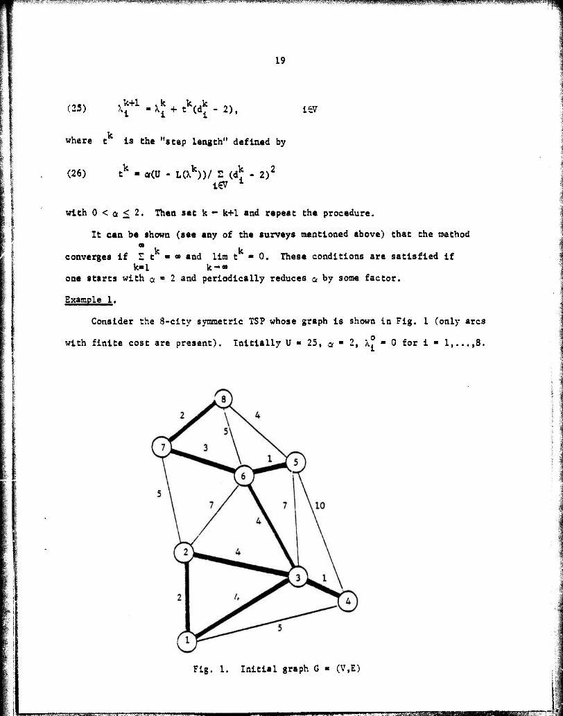
Example 1.

Consider the 8-city symmetric TSP whose graph is shown in Fig. 1 (only arcs

. o with finite cost are present). Initially U ■ 25, a - 2, \1 - 0 for i « 1,..., 8.

Fig. 1. Initial graph G - (V,E)

llipilgHiiiiapipjipLiiy^i, I '.....a.^ftWSpgpgpilBJpWftlW^-'g'

20

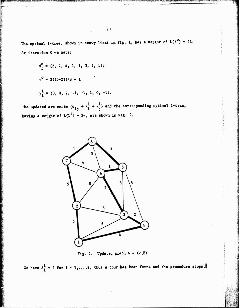
The optimal 1-tree, shown in heavy lines in Fig. 1, has a weight of L(X ) - 21.

At iteration 0 we have:

d[ - (2, 2, 4, 1, 1, 3, 2, 1);

t° - 2(25-21)/8 - 1;

\J - (0, 0, 2, -1, -1, 1, 0, -1).

The updated arc costs (c±, + \J + \h and the corresponding optimal 1-tree,

having a weight of L(\ ) - 24, are shown in Fig. 2.

Fig. 2. Updated graph G * (V,E)

1 !' We have d « 2 for i ■ 1 8; thus a tour has been found and the procedure stops.i|

1- _t

21

Held and Karp [1971] pointed out that if X° is taken to be, instead of

0, the vector defined by

i I

\± - -<ut + v^/2 , i6V ,

where (u, v) is an optimal solution to the dual of the assignment problem with

costs c.. ■ c ., V i,j, then one always has v(H(X0)) > v(AP). Indeed, for this

choice of \° one has from (23)

L(X°) »min Z Z (c, + X? + X°)x - 2 Z X? x3C(7) i€V j>i 13 x J 1J i€V x

- min Z E rt(c. - u - v ) + (c - u. - v )] + Z (u. + v.) x€x(w") i€V j>i l lJ 1 J ji J 1 i€v i 1

> v(AP),

since v(AP) ■ Z (u + v ) and c. - u - v > 0, ¥ i,j. i&f i 1 ij l J -

This kind of initialization requires of course that one solve AP prior to

addressing problem (24).

Heibig Hansen and Krarup [1974] and Smith and Thompson [1977] distinguish be-

tween the application of the subgradient procedure at the root node of the t

search tree and at subsequent nodes, by using different starting vectors X

and different stopping rules.

Volgenant and Jonker [1982] use an updating formula for X , and an ex-

it pression for t , different from (25) and (26), respectively. Namely, they

It take t to be a positive scalar decreasing according to a series with a

constant second order difference, i.e.

(27) Ml k k-1 2t + t ■ constant,

m^^mmmmmmmmm^fr^'

aiWWHIHi^WlilWWWMiSBJII»*^-'

k+1 and define \ by setting for iSV,

22

PgBWlBBPliHiBilBPWSWBBil ItSOfllWJiJJWBW-IWWWS^M^S»"

(28) kk+l - ( if dJ-2

v \J + 0.6tk(d*-2) + 0.4tk(dJ"l-2) otherwise

It should be mentioned that none of the versions of this subgradient optimization

method can be guaranteed to solve (24) in polynomial time with a prespecified

degree of accuracy. However, the stopping rules are such that after a certain

number of iterations the procedure terminates with an approximation to an

optimal X, which gives a (usually good) lower bound on L(X).

Branching rules

BR 6. (Held and Karp [1971]). At node k, let the free edges of the current

1-tree (i.e. those in E\£-UL ) be ordered according to nonincreasing penalties,

and let the first q elements of this ordered set be j» {(i,,j,) (i_»j„)}»

where q will be specified below. Define q new subproblems by

c+r \ ^W : h * l r-1^ r * 1»""(l

r - l,...,q-l (29) \+r " VJ'(lr»V5 »

*k+q " \ Uf (i»j)j£lk-tq : i - P or j - p}

Here p € V is such that L contains at most one edge incident with

p, while L contains two such edges; and q is the smallest subscript

of an edge in J for which a node with the properties of p exists.

This rule partitions the feasible set, and makes the current 1-tree

infeasible for each of the new subproblems generated, but the number q of

the new subproblems is often larger than necessary.

g ™--TBWI JW« '•'»!»" >u»"* i

3R 7, (Smith and Thompson [1977j). Choose a node whose degree in the

current 1-tree is not 2, and a raaximun-cost edge (i,j) among those incident

with the chosen node. Then generate two new subproblems defined by

Vrt-ikUttt.i». \+l-\ (30)

h+2 ' h ' Ifcrt-IfcUCCLJ)}.

This rule generates only two successors of each node k of the search

tree, but the minimum 1-tree in subproblem k remains feasible for subproblem

k + 2.

BR 8. (Volgenant and Jonker [1982]). Choose a node p whose degree in

the current 1-tree exceeds 2. Such a node is incident with at least two free

edges, say (i^j^) and (i2,J2) (otherwise L contains two edges incident

with p, hence the remaining edges incident with p belong to or should belong

to E, ). Generate three new subproblems defined by

^+1 " h '

(31) \+2 ■■fcUCda.V]

\+3 * h uCc*i.Ji>3

\+i ' h uCd^Jj) . <i2.J2)] ;

^+3"^

If p is incident with an edge in L , then node k+1 is not generated.

This rule also partitions the feasible set and makes the 1-tree at node k

infeasible for each of the successor nodes, while the number of successors of

each node is at most 3.

'!afc.*3CV?VW Tlwa»

■■n; Lmm nm&mggm^imga*;

B^j«MfftWPBWjpiuilMttiiauj[ju.,wgmTO

24

Other features

Held and Karp [1971] and Smith and Thompson [1977] use a depth first sub-

problem selection rule, while Volgenant and Jonker [1982] have implemented both

a depth first and a breadth first rule, with computational results that indi-

cate a slight advantage for the depth first rule (in their implementation).

Extension to the asymmetric TSP

The basic ideas of the 1-tree relaxation of the symmetric TSP carry

over to the asymmetric case (Held and Karp [1970]), in that the 1-tree in

an undirected graph can be replaced by a 1-arborescence in the directed graph

G • (V,A), defined as an arborescence (directed tree) rooted at node 1,

plus an arc (1,1) joining some node i€V\[l3 t0 node !• Tne constraints

defining a 1-arborescence, namely (4) and

(32) S 2 x.. > 1 , VSCV: [1J6S i€Sj€V\S 1J *

(33) S Sx -n i€Vj€V 1J

(34) Ex.. - 1 i€V il

are easily seen to be a relaxation of the constraint set (2), (4), (5) of

the TSP.

The problem of finding a minimum-cost 1-arborescence can again be de-

composed into two independent problems, namely (or) finding a minimum-cost

arborescence in 6 rooted at node 1, and (£) finding a minimum-cost arc

(1,1) in 6. Problem (a) can be solved by the polynomial time algorithms 2

of Edmonds [1967] or Fulkerson [1974], or by the 0(n )-time algorithm of

Tarjan [1977],

attWMWMM ■

25

To obtain the Lagrangean version of the 1-arborescence relaxation, one

forms the function

(35) L(X) « min 2 2 c. .x + 2 X ( 2 x . - 1) x€X(G) i€Vj€V i:i 1J i€V l j€V iJ

»min 2 2 (c + X ) x - EX., x€X(G) i€Vj€V 1J J i€V

where X(C) is the set of incidence vectors of G, the family of 1-arbo-

rescences in 6. Again, the strongest lower bound on v(TSF) is of course

given by X ■ X such that

(36) L(X> = max L(X) , X

and subgradient optimization can be used to solve problem (36), However,

computational experience with this relaxation (see Smith [1975]) shows it to

be inferior (for asymmetric problems) to the AP relaxation, even when the

latter uses the original objective function of the ISP.

4. Relaxation III: the Assignment Problem with Lagrangean Objective Function

This relaxation was used for the asymmetric TSP by Balas and Christofides

[1981], It is a considerable strengthening of the relaxation consisting

of the AP with the original cost function, involving a significant computa-

tional effort, which however seems amply justified by the computational

results that show this approach to be the fastest currently available method

for this class of problems.

Consider the asymmetric TSP defined on the complete directed graph G » (V,A),

in the integer programming formulation (1), (2), (4), plus the subtour-elimination

constraints. The latter can be written either as (3) or as (5), but for reasons

«.

•^hrieWUBW

«SSIIWIIMWHPPPW

26

to be explained later, we include both (3) and (5), as well as some positive

linear combinations of such inequalities, and write the resulting set of subtour-

elimination inequalities in the generic form

(37) mlfa " *° * t € T .

Thus our integer programing formulation of the TSP consists of (1), (2), (4)

and (37). To construct a Lagrangean relaxation of TSP, we denote by X the feasible

set of APf and associate a multiplier w , t<=T, with every inequality in the system

(37). We then have

(38) L(w) » min Z Z ex x£Xi£Vj€V 1J 1J

!»,(! Z a*x. t€T tVi€Vj€7 ijAlj °

« min Z Z (c - S w a )x + Z w a* , x(=Xi€Vj€V 1J t€T C 1J 1J t€T C °

where w * (w ). Clearly, the strongest such relaxation is given by w « w such

that

(39) L(w) - max L(w) w>0

The Lagrangean dual (39) of the TSP could be solved by subgradient optimi-

zation, like in the case of the 1-tree relaxation of the symmetric TSP. However,

in this case the vector w of multipliers has an exponential number of compo-

nents, and until an efficient way is found to identify the components that need

to be changed at every iteration, such a procedure seems computationally

expensive. Balas and Christofides [1981] therefore replace (39) by the

"restricted" Lagrangean dual

(40)

where

max L(w) , wSJ

ÜKT : ~~ 1 ■ "mmm W'xpv^mm

HüffflS»*- "*M#**«HSl!f88p XMm^-ri&iJwa^Mi»J^&^^

27

w w

w > 0 and there exists u,v€R such that

f » c. . if x. - 1 .t ♦ T ♦ z wt. i y _«

J t€T 1J * < c, . if r.ifl - lj ij

I-. '-

1 I

and x is the optimal solution found for the A?.

In other words, (40) restricts the multipliers w to values that,

together with appropriate values u. , v , form a feasible solution to the

dual of the linear program given by (1), (2), (37) and x . > 0 , i,j€V.

This may cause the value of (40) to be less than that of (39), but it

leaves the optimal solution x to AP, also optimal for the objective function

(38). Thus (40) can be solved without changing x. While no good

method is known for the exact solution of (40), Balas and Christofides [1931]

give a polynomially bounded sequential noniterative approximation procedure,

A A

which yields multipliers w such that L(w) typically comes close to v(TSP): t

for randomly generated asymmetric TSP's, L(w) was found to be on the average

99.5% of v(TSP) (Christofides [1979], p. 139-140).

The procedure starts by solving AP for the costs c ., ¥ i,j, and taking ut, v

to be the components of the optimal solution to the dual of AP. It then assigns

values to the multipliers w sequentially, without changing the values assigned

earlier. We say that an inequality (37) admits a positive multiplier, if there

exists a w > 0 which, together with the multipliers already chosen, satisfies

the constraints of W. At any stage, v(TSP) is bounded from below by

(41) Eu, + Ev. + Z »„a l€v j€V 3 t€T

't t '

since (u, v, w) is a feasible solution to the dual of the linear program defined

by (I), (2), (37) and x, > 0, » i,j.

■J3SZ? : ,'". '*i T-SK7

, i ■-■■II, ,i i . . ,. . . .-..,,.--. ,-■'." 'iuu .»I ■■■n'.-M» lain...») ■ n—».« . ~ - ~ «<•*<»*.*«*■

28

The bounding procedure successively identifies valid inequalities that

(i) are violated by the AP solution x , and

(ii) admit a positive multiplier.

Such inequalities are included into L(w) in the order in which they

are found, with the largest possible multiplier w . The inclusion of each

new inequality strengthens the lower bound L(w). We denote by c the re-

duced costs defined by the optimal dual variables u. , v. and the multipliers

V 1-*-*ij-cij -ui-vj - tlTVtr At any given stage, the admissible graph 6 * (V,A ) is the spanning

subgraph of G containing those arcs with zero reduced cost, i.e.

Ao - { (i,j) € A|ttt + Vj + ^ViJ " Cij ; •

where I is the index set of the inequalities included so far in L(w). The

inclusion of each new inequality into the Lagrangean function adds at least one

new arc to the set A . Furthermore, as long as G is not strongly connected, the

procedure is guaranteed to find a valid inequality satisfying (i) and (ii). Thus

the number of arcs in A steadily grows; and when no more inequalities can be

found that satisfy (i) and (ii), G is strongly connected. Finally, if at some

point G becomes Hamiltonian and a tour R is found in G whose incidence v o o

vector satisfies (37) with equality for all t€T such that w > 0, then H is an

optimal solution to TSF (see Exercise 5).

Three types of inequalities, indexed by T, , T, and T- , respectively,

are used in three noniterative bounding procedures applied in sequence. We

will denote the three components of w corresponding to these three inequality

classes, by J. * 0-i)i£T , \t - (u1>lgI «d Y- (Vi€T » res?ecciveiy«

^JHBiWPilK.liltM^'^^IWIiW'J'WWff1

29

3ounding procedure I

This procedure uses Che inequalities (5) satisfying conditions (i) and (ii).

For any SCI, the set of arcs (S,V\S) - {(i,j)€AJi€S, j€v\S} is called a directed

cutset. The inequalities (5) corresponding to the node sets S , t€T, can be

represented in terms of the directed cutsets K ■ (S , V\S ), as C C t

(42) I x.. > 1, t € I- . (i,J)€Kt

1J

At any stage of the procedure, the inequality corresponding to cutset

K is easily seen to satisfy conditions (i) and (ii) if and only if

(43) K,?Ä * 0 . c o

To find a cutset K satisfying (43), one chooses a node i € V and

forms its reachable set R(i) ■ fj€VJthere is a directed path from i to j} in

G . If R(i) « V, there is no cutset K with 1 £S satisfying (43), so one chooses

another node. If R(i) # V for some i € 7, then K£ - (R(i), V\R(i)) satisfies (43),

and the largest value that one can assign to the corresponding multiplier \ with-

out violating the constraints of W is \ * min c . Thus the inequality (i,J)£Kt

1J

(42) corresponding to K is included in L(w) by setting the reduced costs to

c.. »- c. . - \ , (i,J)€K , c.. - c.. otherwise. This adds to A all arcs for ij ij t' *■" t' ij ij o

which the minimum in the definition of \ is attained. The search is then started

again for a new cutset; and the procedure ends when the reachable set of every

node is V. At that stage G is strongly connected, and KflA # 0 for all o o

directed cutsets K in G. Also, from (41) and the fact that aC « 1, ¥ tST., it

follows that procedure 1 improves the lower bound on v(TSP) by £ X , i.e., at

the end of procedure 1 the lower bound is

B. - v(AP) + I v .

t€Tl

, ■/» :■-■:,

^^^^lllflflffB^nffSmf'^^^r'r^^Tfrr^ ww^mmmui!hili..mmmmm?mwm*im fggga^

30

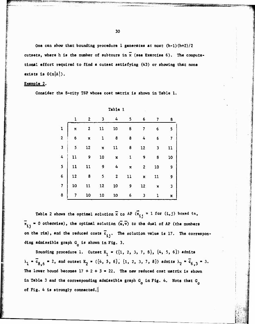
One can show that bounding procedure 1 generates at most (h-l)(h+2)/2

cutsets, where h is the number of subtours in x (see Exercise 6). The computa-

tional effort required to find a cutset satisfying (43) or showing that none

exists is O(nJAJ).

Example 2.

Consider the 8-clty TSP whose cost matrix is shown in Table 1.

1

2

3

4

5

6

7

8

Table 1

3 4 5

x 2 11 10 8 7 6 5

6 X 1 8 8 4 6 7 t

5 12 X 11 8 12 3 11

11 9 10 X I 9 8 10

11 11 9 4 X 2 10 9

12 8 5 2 11 X 11 9

10 11 12 10 9 12 X 3

7 10 10 10 6 3 1 X

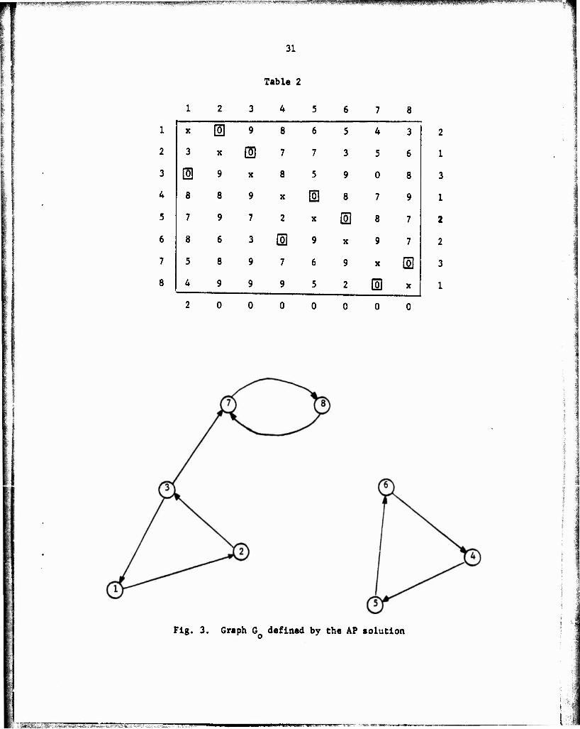
Table 2 shows the optimal solution x to AP (x. = 1 for (i,j) boxed In,

x. ■ 0 otherwise), the optimal solution (u,v) to the dual of AP (the numbers

on the rim), and the reduced costs c... The solution value is 17. The correspon-

ding admissible graph G is shown in Fig. 3.

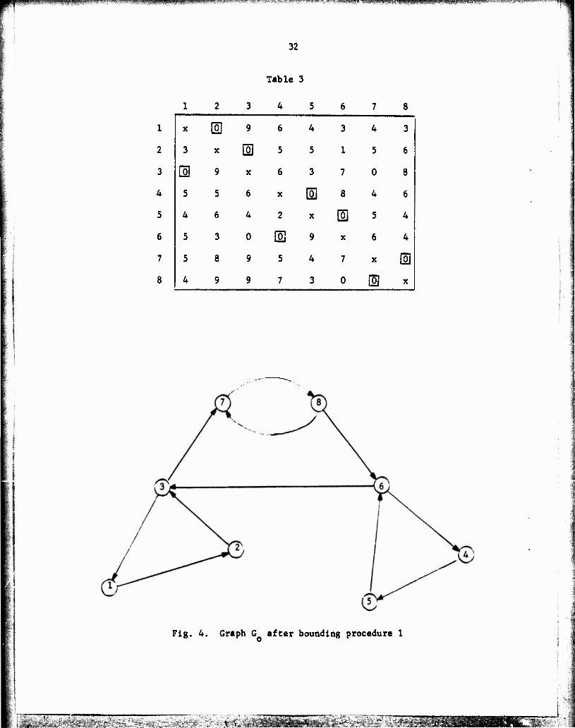
Bounding procedure 1. Cutset K- » ((I, 2, 3, 7, 8}, [U, 5, 6}) admits

^ « Cj 6 ■ 2, and cutset K2 ■ ([4, 5, 6}, (l, 2, 3, 7, 8}) admits X2 ■ cfi 3 - 3.

The lower bound becomes 17 + 2 + 3 ■ 22. The new reduced cost matrix is shown

in Table 3 and the corresponding admissible graph G in Fig. 4. Note that G

of Fig. 4 is strongly connected.||

^^mwf^^^^^is^^w^ ?*qESh{'WWftP^

31

Table 2

1

2

3

4

5

6

7

8

X eg 9 8 6 5 4 3

3 X 0 7 7 3 5 6

® 9 X 8 5 9 0 8

8 8 9 X Bfl 8 7 9

7 9 7 2 X 13 8 7

8 6 3 H 9 X 9 7

5 8 9 7 6 9 X ID 4 9 9 9 5 2 GO X

2

1

3

1

2

2

3

1

Fig. 3. Graph GQ defined by the AP solution

m 'äfe-- JW « Wffg*Wfc- MSMifffwec^ ^

g^pgppKSBBP^fppjSKS'pi'W^ j.-i?i!BI.;_L »'ßl^mglS^i^lllllK^S^MIgW^lll^flffW^!^1^'

32

Table 3

1

2

3

4

5

6

7

8

1 2 3 4 5 6 7 8

X GD 9 6 4 3 4 3

3 X El 5 5 1 5 6

® 9 X 6 3 7 0 8

5 5 6 X (3 8 4 6

4 6 4 2 X BD 5 4

5 3 0 E 9 X 6 4

5 8 9 5 4 7 X @

4 9 9 7 3 0 m X

Fig. 4. Graph G after bounding procedure 1

,ll&r'™ ' ' »■> . '. ->^<^

'"-i.-jvsjgmpimpiijj!—— - - - • -"■ - * ■ i^i»<g^M^--#Pi#iMi)MM^^gm^

33

Bounding procedure 2

This procedure uses the inequalities (3) that satisfy conditions (i) and

(ii), i.e. are violated by x and admit a positive multiplier. To write these

inequalities in the general form (37), we restate them as

(44) - S S x,. >1 - |SJ, t € T, . i€StJ€St

1J c

The subtour elimination inequalities (3) (or (44)) are known to be

equivalent to (5) (or (42)). Nevertheless, an inequality (44) may admit a

positive multiplier when the corresponding inequality (42) does not. and vice

versa.

If S.,...,S. are the node sets of the h subtours of x, every in-

equality (44) defined by S , t»l,...,h, is violated by x; but a positive

multiplier p can be applied without violating the condition that x., ■ 1

implies c . ■ 0, only by changing the values of some u. and v. , and this

in turn can only be done if a certain condition is satisfied. Roughly speaking,

we have to find a set of rows I and columns J such that, by adding to each u., i€l

and v., j€j the same amount y, > 0 that is being added to c.,, (i,j)£(S , S ),

we obtain a new set of reduced costs c' such that c. > 0 for all (i,j), and

c' » 0 for all those (i,j) such that x.. ■ 1. The condition for this is best

expressed in terms of the assignment tableau of the Hungarian algorithm vh<»se

rows and columns are called lines. and whose row/column intersections are called

cells. Cells correspond to arcs of G and are denoted the same way.

Let S be the node set of a subtour of x, and

K - C(i.J)€AjiJ€St}, A'c - [(i.J^Jx^ - 1]

—g—na^g

w.»*atsj("y,»jujiii^..ul- .'- '■'- ■■'-"■" -w!. ...JJOIL;41|!I.!!LHI,IWI I 11,15«—!-.—=!-«— -. - - - - ^"aiBgBM^jf#MM«g#;#™ywa^

34

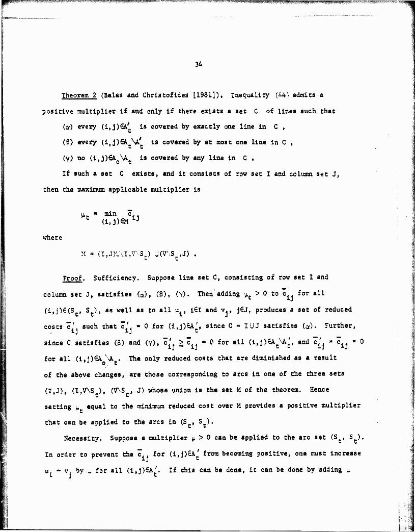
Theorem 2 (Balas and Christofides [1981]), Inequality (A4) admits a

positive multiplier if and only if there exists a set C of lines such that

(a) every (i,J)€k' is covered by exactly one line in C ,

(3) every (i,j)€A \A' is covered by at most one Una in C , t t

(y) no (i,j)€A \A is covered by any line in C .

If such a set C exists, and it consists of row set I and column set J,

then the maximum applicable multiplier is

u - min c C (i,j)€M 1J

where

M - (I,J)'.a,VS,) v(v\st,j) .

Proof. Sufficiency. Suppose line set C, consisting of row set I and

column set J, satisfies (a), (g), (v). Then adding ^ > 0 to c for all

(i,j)€(S , S ), as well as to all u , i€l and v., j€j, produces a set of reduced

costs c' such that c' - 0 for (i,j)€A^, since C - IUJ satisfies (a). Further,

since C satisfies (ß) and (y), e' > c « 0 for all (i, j)^^, and c^ - c^ - 0

for all (i,j)€A V>A . The only reduced costs that are diminished as a result

of the above changes, are those corresponding to arcs in one of the three sets

(I,J), (I,V\S ), (V\S , J) whose union is the set M of the theorem. Hence

setting u equal to the minimum reduced cost over M provides a positive multiplier

that can be applied to the arcs in (St, St).

Necessity. Suppose a multiplier (j. > 0 can be applied to the arc set (St> St).

In order to prevent the c for (i,j)€A' from becoming positive, one must increase

u. * v by „ for all (i,j)€A'. If this can be done, it can be done by adding _

'^"^ "■■■'^ulSiSEEIs ^'^««»^^

35

to u. or v (but not to both) for (l,j)€A'j «nd the corresponding Index sets I

and J form a set C • IUJ that satisfies (or). Let C be the collection of all

sets C obtained In this way. Now take any C€C. If C violates (ß), then

c' ■ c. + p. - 2p, < c. » 0 for some (i,J)€AAA' and If it violates (Y), then lj lj ij c »

c' < c. ■ 0 for some (i,j)€A \Afc. Since by assumption y, > 0 can be applied

to (S , S ), there exists at least one set C6C that satisfies both (ß) and (v).||

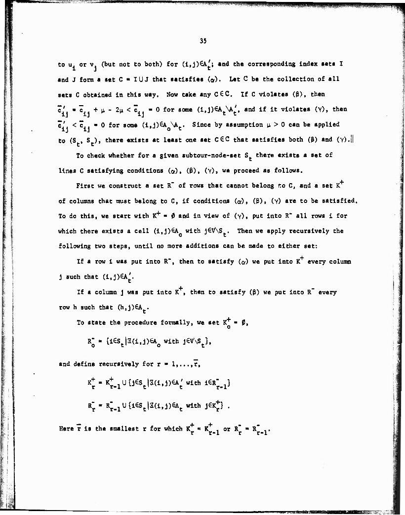
To check whether for a given subtour-node-set S there exists a set of

lines C satisfying conditions («), (ß), (v), we proceed as follows.

First we construct a set R of rows that cannot belong r.o C, and a set K

of columns that must belong to C, if conditions (g), (ß), (v) are to be satisfied.

To do this, we start with K+ ■ j9 and in view of (v), put into R" all rows 1 for

which there exists a cell (i,j)€A with j€V\S . Then we apply recursively the

following two steps, until no more additions can be made to either set:

If a row i was put into R", then to satisfy (a) we put into K every column

j such that (i,j)€A^.

If a column j was put into K , then to satisfy (ß) we put into R~ every

row h such that (h,J)€A .

To state the procedure formally, we set K ■ 0,

r - [l6St|a(i.J)6Ao with j6V\St},

and define recursively for r ■ l,...,r,

Kr " Kr-lU ܣSt|3(i,j)6At' with 1^^}

Rr " Rr-lU£i6Stla(1'J)€At wlth J€K? '

Here r is the smallest r for which K ■ K , or R* ■ R~ ,. r r-1 r r-1

- . -i «HI J'-J.t JIM

36

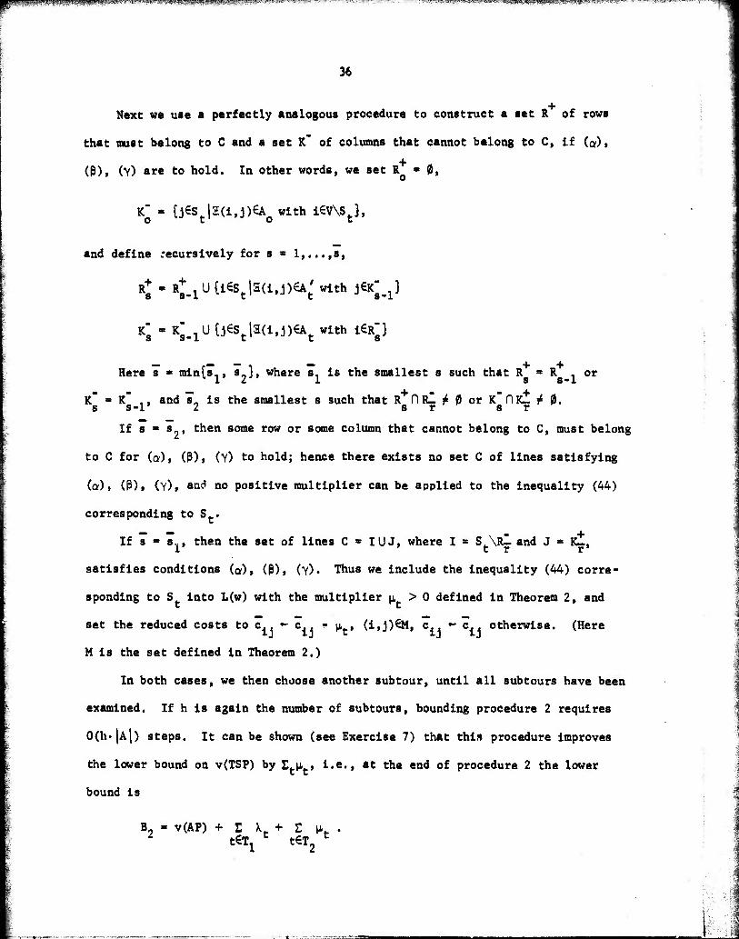
Next we use a perfectly analogous procedure to construct a set R of rows

that must belong to C and a set K" of columns that cannot belong to C, If (#),

(ß)t (Y) are to hold. In other words, we set R « 0,

if - {j€St|2(i,j)€Ao with i€V\St),

and define recursively for s « l,...,s,

Rs" * R8-lUti€Stla(i'j)6At wlth j6Ks-l}

Ks * Ks-lU tj^Stl3<i,j)€At with 16R;)

Here s * mints., s_), where s, is the smallest s such that R = R , or 1 1 2J' 1 s s-1

R ■ K ,, and s„ is the smallest s such that R 0 R_ £ (9 or K PlK- + 0. s s-1 Z s r s r

If s ■ s-, then some row or some column that cannot belong to C, must belong

to C for (a), (3), (V) to hold; hence there exists no set C of lines satisfying

(a), (ß), (Y)> and no positive multiplier can be applied to the inequality (44)

corresponding to Sfc.

If s » s.,, then the set of lines C ■ IUJ, where I - SARI and J ■ R_, i. ' t r r'

satisfies conditions («), (ß), (y). Thus we include the inequality (44) corre-

sponding to S into L(w) with the multiplier (j, > 0 defined in Theorem 2, and

set the reduced costs to c.. «- c.. - p, , (i,j)€M, c.. «- c.. otherwise. (Here

M is the set defined in Theorem 2.)

In both cases, we then choose another subtour, until all subtours have been

examined. If h is again the number of subtours, bounding procedure 2 requires

0(h'|A|) steps. It can be shown (see Exercise 7) that this procedure improves

the lower bound on v(TSP) by Et^t» i.e., at the end of procedure 2 the lower

bound is

B, - v(AP) +1 v + I u 2 t€Tx

t t€T2 C

I^-V^^Wr-fi!^-. ^^^SS^^^^^^^^^^B^^^^^W^^^^^M

37

ü f

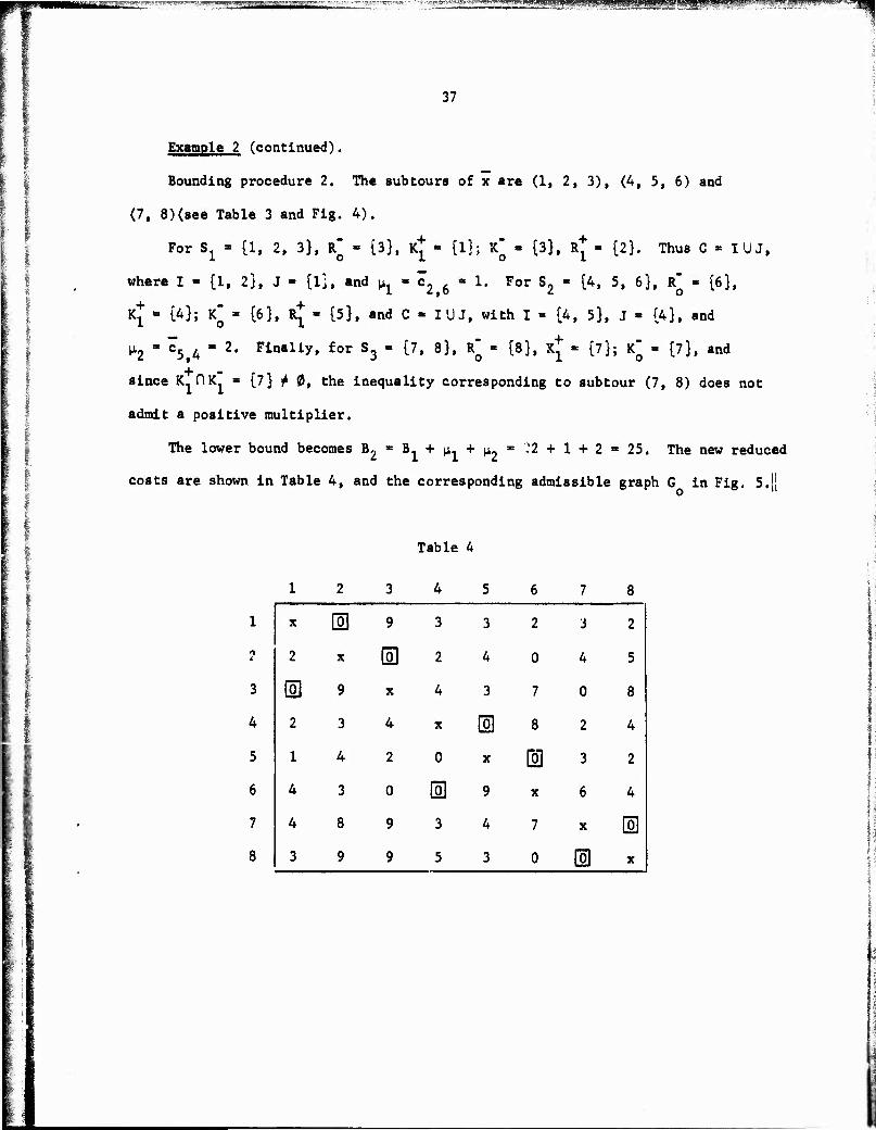
Example 2 (continued).

Bounding procedure 2. The subtours of x are (1, 2,3), (4, 5, 6) and

(7, 8)(see Table 3 and Fig. 4).

For Sx » (1, 2, 3}, if « {3}, K+ - {l}; if - {3}, R+ - {2}. Thus C * IUJ,

where I ■ {l, 2}, J - [l], and |A_ - c"2 g « 1. For S2 - {4, 5, 6}, R* - {6},

Kl " t43; Kö " i6^» >i * W* and C - IUJ, with I - {4, 5}, J - {4}, and

^2 " *5,4 " 2* Finaliy» £or S3 " t7» 8}, R^ - [8}, X+ « {7}; if - [7}, and

since K. PlK = {7} t 0, the inequality corresponding to subtour (7, 8) does not

admit a positive multiplier.

The lower bound becomes B,. ■ B, + M,, + jj,2 ^ -2 + 1 + 2 « 25. The new reduced

costs are shown in Table 4, and the corresponding admissible graph G in Fig. 5,j|

Table 4

3

4

5

6

7

8

1 2 3 4 5 6 7 8

X 0 9 3 3 2 3 2

2 X 0 2 4 0 4 5

GO 9 X 4 3 7 0 8

2 3 4 X m 8 2 4

1 4 2 0 X © 3 2

4 3 0 13 9 X 6 4

4 8 9 3 4 7 X d 3 9 9 5 3 0 m X

gigi»»jjiwti^

'

38

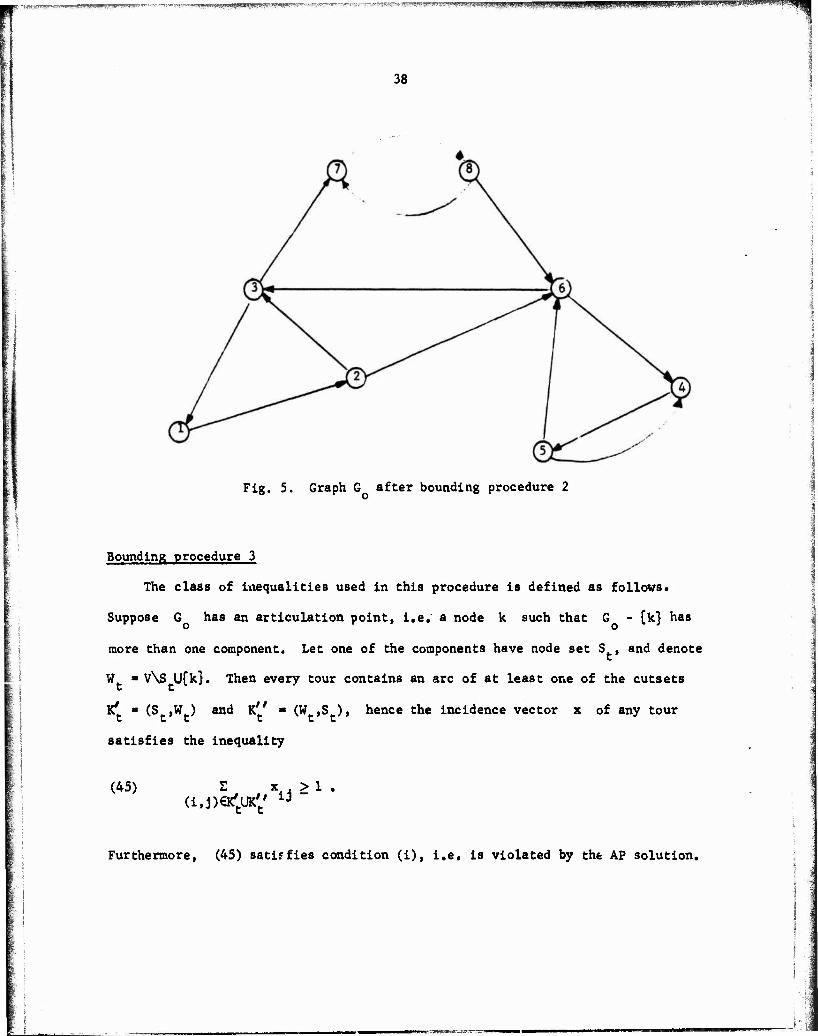
Fig. 5. Graph G after bounding procedure 2

Bounding procedure 3

The class of inequalities used in this procedure is defined as follows.

Suppose G has an articulation point, i.e. a node k such that G - {k] has

more than one component. Let one of the components have node set S , and denote

W ■ V\S Ufk}. Then every tour contains an arc of at least one of the cutsets

¥f ■ (S ,W ) and K'' ■ (W ,S ), hence the incidence vector x of any tour

satisfies the inequality

(45) a,i)&?t\M't it ij -

> 1 .

Furthermore, (45) satisfies condition (i), i.e. is violated by the AF solution.

■BSjgwglJSIIBjaBps; ■'waHWWWjiWPW^UgiilJttWl1 gpgpwpwigwwpwpaftB ^ LIUII !

39

Bounding procedure 3 uses those inequalities (45) that also satisfy

condition (ii). Although every inequality (45) is the combination of some

inequalities (3) and equations (2) (see Exercise 8), nevertheless it is possible

to find inequalities (45) that satisfy condition (ii), i.e., admit a positive

multiplier, when no inequality (3) (i.e., (44)) satisfies it. Indeed, it is not

hard to see, that if k is an articulation point of G and S is the node set of

one of the components of G - {k}, then K'DA = K'' 0 A ■= 0 and a positive

multiplier given by

(46) v ■ min c (i.jXS'j.UK'/ iJ

can be applied to the arc set K'UK'' . On the other hand, if G has no articula- t t o

tion point, then for any choice of the node k, the minimum in (46) is 0 and thus

no inequality (45) admits a positive multiplier.

Thus bounding procedure 3 checks for ««*ry iCV whether it is an articulation

point, and if so, it takes the corresponding inequality (45) into L(w) with the

multiplier v given by (46). This is done by setting c - c - v , (i, J)€K'UK" ,

c.. *- c. otherwise. Since G has n nodes, and testing for connectivity requires

0(|A|) steps, bounding procedure 3 requires 0(n|AJ) steps.

In view of (41) and the fact that (45) has a righthand side of 1, at the end

of bounding procedure 3 one has the following lower bound on v(TSP):

B » v(AP) + £ X + S n + I v . 1 t€Tx

C t€T2 C t€T3

C

Example 2 (continued).

Vertex 6 is an articulation point of G (see Fig. 5). The corresponding

cutsets are K^ * ({4, 5}, {l, 2, 3, 7, 8}) and K^'- ({1, 2, 3, 7, 8}, {4, 5}),

iiiMi'iWIIJM ^wig«j.ffj^Bi#»iwp^

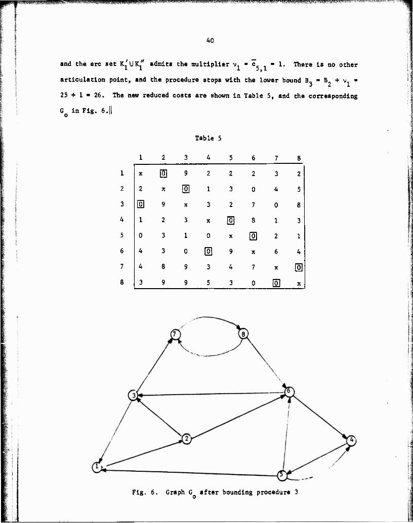
40

and the arc set K^UK/' admits the multiplier v. - e - 1. There is no other

articulation point, and the procedure stops with the lower bound B, = B9 + v.. »

25 + 1 • 26. The new reduced costs are shown in Table 5, and the corresponding

GQ in Fig. 6.||

Table 5

1

2

3

4

5

6

7

8

1 2 3 4 5 6 7 8

X 0 9 2 2 2 3 2

2 X IS 1 3 0 4 5

H 9 X 3 2 7 0 8

1 2 3 X m 8 1 3

0 3 1 0 X 0 2 1

4 3 0 m 9 X 6 4

4 8 9 3 4 7 X 0 3 9 9 5 3 0 m X

Fig. 6. Graph G after bounding procedure 3 o

p^npsssspiHiBMiiMsspi^^

t I f

41

I Additional bounding procedures

At the end of bounding procedure 3, G is strongly connected and without

articulation points. At that stage an attempt is made to find a tour in G .

For that purpose a specialized implicit enumeration technique is applied,

with a cut-off rule. If a tour H is found whose incidence vector x satis-

fies with equality all those inequalities (37) such that wt > 0, then H is

optimal for the current subproblem (this follows from elementary Langrangean

theory).

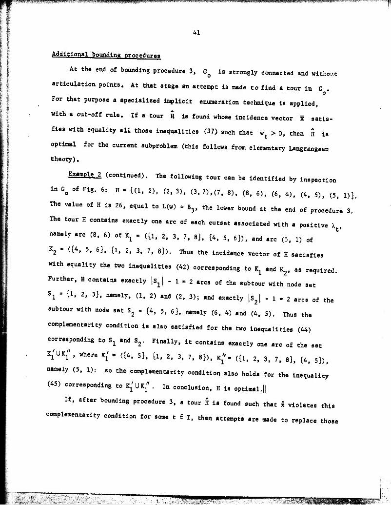
Example 2 (continued). The following tour can be identified by inspection

in Go of Fig. 6: H = ((1, 2), (2, 3), (3, 7),(7, 8), (8, 6), (6, 4), (4, 5), (5, 1)},

The value of H is 26, equal to L(w) ■ B,, the lower bound at the end of procedure 3.

The tour H contains exactly one arc of each cutset associated with a positive \ ,

namely arc (8, 6) of ^ = ({l, 2, 3, 7, 8}, (4, 5, 6}), and arc (5, 1) of

K2 - ({4, 5, 6}, [1, 2, 3, 7, 8}). Thus the incidence vector of H satisfies

with equality the two inequalities (42) corresponding to K. and K., as required.

Further, H contains exactly |s.| - 1*2 arcs of the subtour with node set

S^ * {l, 2, 3}, namely, (1, 2) and (2, 3); and exactly |sj -1=2 arcs of the

subtour with node set S„ ■ {4, 5, 6}, namely (6, 4) and (4, 5). Thus the

complementarity condition is also satisfied for the two inequalities (44)

corresponding to S, and S.. Finally, it contains exactly one arc of the set

K^UK^', where K^ « ({4, 5}, £l. 2, 3, 7, 8}), Kj"» ({l, 2, 3, 7, 8}, {4, 5}),

namely (5, 1): so the complementarity condition also holds for the inequality

(45) corresponding to K'UK.". In conclusion, H is optimal.||

If, after bounding procedure 3, a tour H is found such that x violates this

complementarity condition for some t 6 T, then attempts are made to replace those

i'0&M\::..^^?\;-^-}*a^c■-■ ',-UW^7- < ' ,m^^mmmmmm

lim^seji^MPggW^ ' a " " ^.■y^.^??ra^*^^^ "T" --—'■»-"■■" ■■.■■■■■■■ -i » i,_.,LMi^h. iu. J WW,, ,i: .JL ."JI L*JIJ.»-.■.IJ.W' !?M^

42

inequalities (37) that are "out of kilter," i.e., for which the complementarity

condition is violated, by "in kilter" inequalities (of the same type), i.e.,

inequalities that are tight for x and thus admit positive multipliers satisfying

the complementarity condition. These attempts consist of a sequence of three

additional bounding procedures, called 4, 5 and 6, one for each type of inequality

(42), (44) and (45), respectively. Bounding procedure 4 takes in turn each in-

equality (42) which has a positive multiplier X and yet is slack for x, and per-

forms an exhaustive search for other inequalities of type (42) that could replace

the inequality in question (with new multipliers) and which are tight for x. If

the search is successful, the in kilter inequalities with their new multipliers f

1 replace the out of kilter inequality and one proceeds to the next out of kilter

inequality of type (42). Procedures 5 and 6 perform the same function for out

of kilter inequalities of type (44) and (45), respectively. These procedures are

described in detail in Balas and Christofides [1981]. When procedures 4, 5 and

6 are not successful in replacing all out of kilter inequalities (and thus proving

H to be an optimal tour), they nevertheless strengthen the lower bound on v(TSP).

Each of the six bounding procedures is polynomially bounded. This (worst

4 3 case) bound is 0(n ) for procedure 1, 0(n ) for each of the other procedures.

The mean times are considerably shorter, and on the average procedure 2 (the

| only one that changes the dual variables u , v ) takes the longest. The

general algorithm of course remains valid if any subset of ehe six bounding

procedures is used in place of the full set, but computational testing indi-

cates that using all 6 procedures is more efficient (i.e. results in smaller

search trees and shorter overall computing times) than using any proper subset.

^mmmmmmmmms. '■■ '" '."..".'.'".I'l."!11,1»! *—~——————————°- "■■»■ ■ ■■ IIJ™IIIJ™II«IIII«IIJIJMM^^

43

Branching rules and other features

Before branching, all arcs (i,j) such that c.. > U - L(w) are deleted

from G. This "reduction" has removed on a set of 120 randomly generated problems

(Balas and Christofides [1981]), on the average 96-97% of the arcs in problems

with up to 150 variables, and 98% in problems with 175-325 variables.

The AP relaxation with Lagrangean objective function can of course be used

with any of the branching rules BR1 - BR5 described in the context of the AP

relaxation with objective function (1). Balas and Christofides [1981] use two

rules intermittently, namely BR3 (partitioning on the basis of a subtour elimi-

nation inequality (3)), and another rule based on a disjunction from a condi-

tional bound, introduced earlier in the context of set covering (3alas [1980]).

This latter rule is motivated by the following considerations. A

Let H be the current tour and x its incidence matrix. Remove from L(w)

all those inequalities (37) that are slack while the associated multiplier is

positive. Let c be the reduced costs, and L(w) the lower bound, resulting

from this removal.

Theorem 3. Let S=H, S « ((i^ j^ (i j )} be such that

P (47) Je >U - L(w),

r«l r r

and let the arc sets Q CA, r ■ l,...,p, satisfy

(48) > c <c , (i,j)6A r|U,j)=Qr Vr

ij

Then «very solution x to TSP such that ex <. U satisfies the disjunction

(49) p

r» ' (*u " 0, (i,j)€Q ) '1 - r

MPpqppppn^PPPpggg^gP^ICT^lJUi.IVMIunil.llllulliliWlllWiiHXil >p«<WHn^BPmi*igwpa«!ff«l«IUIW^>"»l J

44

Proof. L(w) is the value of an optimal solution to the dual of the linear

program LP defined by (1), (2), x > 0, (i,j)€A, and those inequalities (37)

with a positive multiplier. Now let x be a feasible solution to LP that violates

(49). Then x satisfies

(50) S___Zx..>l , r - l,...,p. U,J)€Q. iJ

r

Let LP be the linear program obtained by adding to LP the constraints (SO).

From (48), if we assign the values c. . , r ■ l,...,p to the dual variables rJr

associated with the inequalities (50), we obtain a feasible solution to the dual

P A of LP.. But then the objective function value of this solution is L(w) + Ec. . ,

r=l rJr and hence from (47)

ex > L(w) + ECj , > U. r=l r r

Thus every solution x to TSP such that ex < U satisfies (49).!|

The branching rule can now be stated as follows.

BR9. Choose a minimum-cardinality set SCH, S - {(i-, U),...,(i , j )},

satisfying (47). Next construct a px|A| 0-1 matrix D * (df4) (where r is the

row index and (i,j) the column index), with as many l's in each column as possible,

subject to the condition (48) and (i , j )6Q t r = l,...,p, where

Qr * tU.jXJAJdJj = 1}.

Generate the p new subproblems defined by the disjunction (49), where

/ei th

the r- subproblem is given by

(51> | r- 1 p .

h*mh j

«UVMamMMMMAaMM mmmmKmmmmmfiwmmimmmmmmmmmmmmm

45

i 1 ■ i

The branching rule BR9 is used intermittently with BR3 because at different

nodes the ranking of the two rules (in terms of strength) may be different. The

choice is based on certain indicators of relative strength.

As to subproblem selection, the Balas-Christofides algorithm uses a mixture

of depth first and breadth first: a successor of the current node is selected

whenever available; otherwise the algorithm chooses a node k that minimizes

the function

BOO - (L(w)k - v(AP)) |t$V,(te)|

where Mw)k is the value of L(w) at node k, v(AP) is the value of the initial AP,

while 3(0) and s(k) are the number of subtours in the solutions to the initial

AP and the one at node k, respectively.

5. Other Relaxations

For the same reasons as in the case of the AP relaxation with the original

objective function, the AP relaxation with the Lagrangean objective function is

inefficient (weak) in the case of the symmetric TSP. Limited computational

experience indicates that on the average the bound L(w) attains about 967,

of v(TSP), which compares unfavorably with the bound obtained from the 1-tree

relaxation.

On the other hand, the main reason for the weak performance of AP-based

ralaxations in the case of symnetric problems, namely the high frequency of

subtours of length 2 in the optimal AP solution, can be eliminated if AP is

replaced by the 2-matching problem in the undirected graph G - (V,E).

"*f.JW" "jwviuo-mii»! i j^,ai, ^ ^mimmijyijLjiin. pijuii ~-—— J ''«wwwijfti>wyB#uifc.^^

46

The 2-natching relaxation

The problem of minimizing the function (6) subject to constraints (7) and

(9) is known in the literature as the 2-matching problem, and is obviously

a relaxation of the ISP, Bellmore and Malone [1971] have used it for the

symmetric TSP in a way that parallels their use of the AP-relaxation for the

asymmetric TSP. A 2-matching is either a tour or a collection of subtours,

and the branching rules BR2 - BR5 based on the subtour-elimination inequalities

(3) and (5) for the asymmetric TSP have their exact parallels in branching rules

based on the subtour elimination inequalities (8) and (10) for the symmetric TSP.

The objective function (6) can be replaced, just like in the case of the

AP relaxation, with a Lagrangean function using the inequalities (S) and/or

(10), The Lagrangean dual of the TSP formulated in this way is as hard to

solve exactly as in the asymmetric case, but it can be approximated by a pro-

cedure similar to the one used by Salas and Christofides [1981] with the

AP-telaxation. Further facet defining inequalities, beyond (8) and (10),

based on the work of Grotschel and Padberg [1979], can be used to enrich the

set drawn upon in constructing the Lagrangean function.

Although the 2-matching problem is polynomially solvable (Edmonds [1965]),

the main impediment in the development of an efficient branch and bound proce-

dure based on the 2-matching relaxation has so far been the absence of a good

implementation of a weighted 2-matching algorithm. However, as this difficulty

is likely to be overcome soon, the 2-matching relaxation wich a Lagrangean

objective function will in all likelihood provide bounds for the symmetric TSP

cottroarable to those obtained from the 1-tree relaxation.

. li i MnMMBKS

«stp^ipiisigsgwrei'ewsvri^ftw^

47

The n-path relaxation

The problem of minimizing (1) subject to the constraint that the solution

x be the incidence matrix of a directed n-path starting and ending at a fixed

node v (where "path" is used in the sense of walk, i.e., with possible repeti-

tions of nodes, and n denotes the length of the path) is clearly a relaxation

of the TSP. An analogous relaxation of the symmetric ISP can be formulated in

terms of n-paths in the associated undirected graph. Furthermore, the constraints

(2) in the asymmetric case, or (7) in the symmetric case, can be used to replace

the objective function (1) or (6), respectively, by a Lagrangean function of the

same type as the one used with the 1-arborescence and 1-tree relaxations. This

family of relaxations of the TSP was introduced by Houck, Picard, Queyranne and

Vamuganti [19^7]. The (directed or undirected) n-path problems involved in this

3 relaxation can be solved by a dynamic programming recursion in 0(n ) steps.

Computational experience with this approach seems to indicate (Christofides [1979],

p. 142) that the quality of the bound obtained is comparable to the one obtained from

the 1-arborescence relaxation in the asymmetric case, but slightly weaker than

the bound obtained from the 1-tree relaxation in the symmetric case. Since

solving the 1-tree and 1-arborescence problems is computationally cheaper than

solving the corresponding n-path problems, this latter relaxation seems to be

dominated (for the case of the "pure" TSP) by the 1-tree or 1-arborescence re-

laxation. However, the n-path relaxation can easily accommodate extra condi-

tions which the 1-tree and 1-arborescence relaxations cannot, and which often

occur in problems closely related to the TSP (traveling salesman problems with

side constraints appear in vehicle routing (see Chapter 12 of this book) and

other practical contexts.)

imtmriii u — '——■»■—'■

iWW»JWlWi-— - -■_ - - ,-,, _

48

A substantial generalization of the n-path relaxation, due to Christofides,

Mingozzi and loth [1981] and called state-space relaxation, has the same

desirable characteristics of being able to easily accommodate side constraints.

The LP with cutting planes as a relaxation

Excellent computational results have been obtained recently by Crowder

and Padberg [1980] for the symmetric TSP by a cutting plane/branch and bound

approach. It applies the primal simplex method to the linear program defined

by (6)i (7)> x >0, Vi,j, and an unspecified subset of the inequalities ij

defining the convex hull of incidence vectors of tours, generated as needed

to avoid fractional pivots. The procedure uses mostly inequalities of the

form (10), but also other facet inducing inequalities from among those intro-

ii

duced by Grotschel and Padberg [1979], When the 3earch for the next inequality

needed for an integer pivot fails, the procedure branches. Since the main

feature of this approach is the identification of appropriate inequalities to

be added to the linear program at each step, it is being reviewed in the

chapter on cutting plane methods.

6. Performance of State of the Art Computer Codes

In this section we review the performance of some state of the art branch

and bound codes for the TSP, by comparing and analyzing the computational results

reported by the authors of these codes.

The asymmetric TSP

The three fastest currently available computer codes for the asymmetric TSP

seem to be those of Balas and Christofides [1981], Carpaneto and Toth [1580]

and Smith, Srinivasan and Thompson [1977], to be designated in the following by

3C, CT and 3ST, respectively. The nain characteristics of these codes are summa-

^g»..^^^.^..^,,;.,,. ~~" .< ,;, , -""^" 'ijl' ■ääjaB$$$i/Eh \

zmsmmmmmmmmmmzz— - ._.____:— ' s «ässssäSä

49

rized in Table 6. Table 7 describes the computational results reported by the

authors of the codes. Each of the codes was run on a set of (different) asymmet-

ric TSP's whose costs were independently drawn from a uniform distribution of the

integers in the interval [1,1000], The entries of the table represent averages

for 5 problems (SST), 20 problems (CT) and 10 problems (BC), respectively, in

each class. The number of nodes in the SST column is not strictly comparable

with that in the CT and BC columns, since it is based on counting only those

nodes that were selected for branching and processed. Also, the computing times

are not strictly comparable without a correction, since the CDC 7600 is about 3

times faster than the UNIVAC 1108 and the CDC 6600 (Computer Review, GML Corp.,

Lexington, MA., 1979). The picture that emerges, however, by comparing the

figures within each column, for any of these three codes, is a pattern of growth

in computational effort with problem size, that seems rather modest for a problem

usually viewed as "notoriously intractable". We will discuss the functional

relationship between problem siz^ and computational effort in some detail further

below.

For problems in the range 40 < n < 180, the number of nodes generated by

the BC algorithm is considerably smaller than the corresponding numbers for the

other two algorithms, although CT uses a "breadth first" branching strategy, meant

to minimize the number of nodes generated, at the cost of increased storage

requirements. The reason for this is that the Lagrangean bounding function used

by BC changes the ranking of tours among the assignments, removing from considera-

tion many assignment problems whose value in terms of the original objective

function is higher than that of the optimal TSP, and which therefore must be

processed by the CT algorithm. On the other hand, in the range 200 < n < 240,

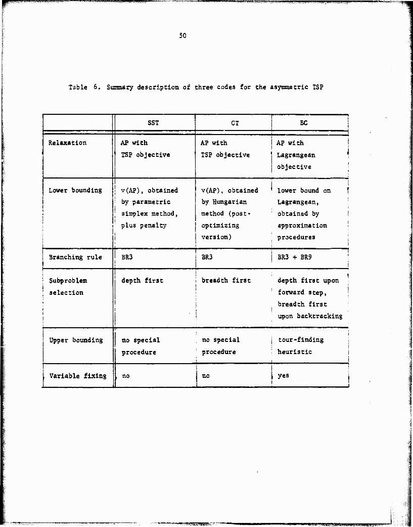
W'Hii "i i 'i" MIM mum\mmmmi^mm^9!mmmmgmKW!K ^^mHwmmmmmm mwmnsmi if \.m mimwmjm I' " "— ■ * ^""-püPPS «Ä*fcf^^-'-=^J

50

Table 6. Summary description of three codes for the asymmetric TSP

SST CT BC

Relaxation AP with

TSP objective

AP with

TSP objective

I AP with I 1 Lagrangean

! objective

Lower bounding v(AP), obtained

by parametric

simplex method,

plus penalty

v(AP), obtained

by Hungarian

method (post-

optimizing

version)

lower bound on

Lagrangean,

obtained by

approximation

procedures

Branching rule BR3 BR3 BR3 + BR9

Subproblem

selection

depth first breadth first depth first upon

forward step,

breadth first

upon backtracking

Upper bounding no special

procedure

no special

procedure

| tour-finding

' heuristic

| Variable fixing no no ! i yes

r&sasammC' ■ mmv;'; agg»snwBf!HSB— tw „■■ ■ ■

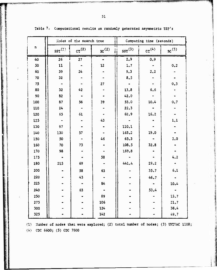
mm^mi¥h&w^y!:''':'^ y-s?s™^JtUl!4ji^ I^IWPSP?!^ mrnmrnm^mmmf^^^^m

51

Table 7. Computational results on randomly generated asymmetric TSP's

1 :bdes of the searc h tree j Computing time (seconds) ,

n SSTV" CT(2) BC(2) j

i

SST(3) i

CTV BC(5) i

40 26 I 27 - 2.9 0.9

i 50 11 - 12 1.7 - 0.2

i 60 39 24 - 9.3 2.2 i

! 70 32 - - 8.5 - -

75 - - 27 - - 0.3

80 32 42 - 13.8 6.6 * i

90 82 - - 42.0 - -

100 87 56 39 53.0 10.4 0.7

110 24 - 22.3 - -

120 65 61 - 62.9 16.2

125 - - 43 . - 1.1

130 97 _ _ 110.1 - -

140 130 57 - 165.2 19.0 -

150 50 - 46 65.3 - 2.0

160 70 73 - 108.5 32.8 -

170 98 - - 169.8 - -

175 - - 58 - - 4.2

180 215 69 - 441.4 29.2 !

200 - 58 63 - 35.7 6.1

220 - 43 - - 46.7 - 1 225 - - 84 i * 10.4

240 - 63 - • 53.4 -

250 - - 89 - - 13.7

275 - - 106 - - 21.7

300 - - 124 - - 38.4

325 - 142 - '

49.7

(1) Number of nodes that were explored; (2) total number of nodes; (3) UN1VAC 1108;

(i) CDC 6600; (5) CDC 7600

—. imnmiwiw- - -^-^wy«uipi.gi^awJw#.feiB »

52

BC yeeras to generate more nodes than CT; the reason for this may be that at

this point the advantage of the "breadth fivst" strategy used by CT outweighs

that of the stronger bounding procedures used by BC. This seems to suggest that

an algorithm basad on the Lagrangean bounding procedures of BC, but using the

"breadth first" node selection strategy of CT, will generate fewer nodes for

any problem size, than either the CT or the BC algorithms. This is undoubtedly

true, but notice that at the current state of the art, the limiting factor in

the use of both algorithms is not computing time (which has never exceeded 1.5

minutes for any problem), but (in core) storage space.

The synmetric ISP

The fastest currently available branch and bound codes for the symmetric TSP

seem to be those of Smith and Thompson [1977] and Volgenant and Jonker [1982],

to be designated in the following by ST and VJ, respectively. Table 8 summa-

rizes their main characteristics, while Table 9 reports on their computational

performance.

Again, each of the two codes was run on a sec of (different) symmetric

TSP's whose costs were indspendently drawn from a uniform distribution of the

integers in the interval [1,1000], The entries of the table represent averages

for 15 problems (except for n-80, where the entry for SST is the average for

5 problems only). The CYBER 750 is about 3 times faster than the UNIVAC 1108.

Both codes were also tested on randomly generated symmetric Euclidean

TSP's, which required for each code a greater computational effort (e.g., for

n » 60 the average number of subgradient iterations was 3049 for ST and

1034 for VJ).

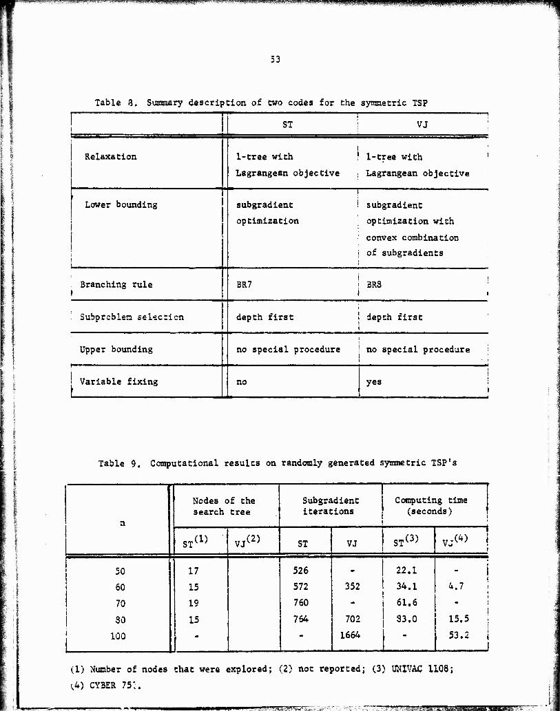
■:n:-7*'mv^^m*^. i ..■li.MmJMmmVH'vvwrnjmM-v - -""•"^P™'»'?W»^l»*mw^^

53

Table 3. Summary description of two codes for the symmetric ISP

1 1

1 ; ST VJ

Relaxation i

1-tree with I 1-tree with '

Lagrangean objective j Lagrangean objective

1

Lower bounding

i I ...■

1 subgradient 1 subgradient

optimization ' optimization with i

i convex combination

j of subgradients

Branching rule 3R7 j 3R8 !

» »

Subprcblen selection depth first ! depch first i

Upper bounding no special procedure no special procedure

Variable fixing no i

yes i

Table 9. Computational results on randomly generated symmetric TSP's

!.

a

Nodes c search

)f the tree

Subgradient iterations

Computing time (seconds)

ST(1) VJ<2> ST « ST(3) VJ<4> ! i

50 17 526 - 22.1 -

60 15 572 352 34.1 4.7

70 19 760 - 61.6 1

I

SO 15 764 702 33.0 15.5 ;

1 10° i

1 - 1664 " 53.2 j 1

(I) Number of nodes that were explored; (2) not reported; (3) 0NIVAC 1108;

(4) CY3ER 75:.

•>—»=*-" ? * ■ iFt-tt^imim&im

B»M»»»!«!»(fc«*H»My«' luiwiiiyitp^i^^

54

Average performance as a function of problem size

TS2 is well known to be NP-complete, hence in all likelihood there is no

polynomial time TSP algorithm, i.e. no algorithm guaranteed to solve every instance

of TSP in a number of steps polynomial in n. However, this statement refers to

the worst case behavior of algorithms, and does not exclude the existence of

algorithms whose performance, though exponential in the worst case, is on the

average polynomial in a. To make the colloquial term "on the average" more

precise, assume the costs c.. of TSP are random numbers drawn inde-

pendently from a uniform distribution over the unit interval. Whether the

expected time required to solve such a problem is an exponential or polynomial

function of n, is at present an open question, on which the opinion of experts

is divided (see, for instance, Bellmore and Malone [1971], and Lenstra and

Rinnooy Kan [1978]).

While the theoretical issue remains unsolved, it is not irrelevant to

examine from this point of view the empirical performance of some of the more

efficient algorithms on randomly generated TSP's. In a recent study, Balas,

McGuire and Toth [1983] have fitted three different approximating curves to the

data of Table 7 for each of the three codes SST, CT and BC for the asymmetric

TSP, in an attempt to determine which of the three types of functions describes

best the behavior of each algorithm. The data of Table 7 were corrected for the

difference in speed between the CDC 7600 and the other two computers by multiplying

by 3 the computing times reported for the Balas-Christofides code. The functions

examined were:

B f(n) - an

f(n) » an Plogn

f(n) « ae ßn

(polynomial),

(superpolynomial).

(axponential),

where log stands for the natural logarithm and e for Its base.

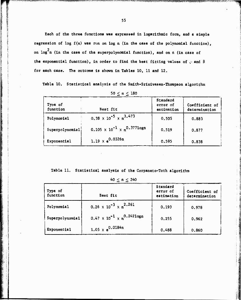
^sswswpigs?^?

55

Each of the three functions was expressed in logarithmic form, and a simple

regression of log f(n) was run on log n (in the case of the polynomial function),

2 on log n (in the case of the superpolynomial function), and on n (in case of

the exponential function), in order to find the best fitting values of c and 0

for each case. The outcome is shown in Tables 10, 11 and 12.

Table 10. Statistical analysis of the Smith-Srinivasan-Thompson algorithm

50 < n < 180 1

Type of function Best fit

' ■ •""' ■■■' i

Standard error of estimation

Coefficient of determination

Polynomial -5 3.473

0.38 X10 3 X n ' 'J 0.505 0.883

Superpolynomia1 0.105 x 10"1 X n°-3771°8n 0.519 0.877

Exponential 1.19 X e°-0326n 0.595 0.838 j

I .1

Table 11. Statistical analysis of the Carpaneto-Toth algorithm

40 < n < 240

Type of function Best fit

Standard error of estimation

Coefficient of determination

Polynomial 0.26 X 10"3 X n2*261 0.193

1

0.978

Superpolynomia1 0.47 X IQ"1 x n°-2421o*n 0.255 0.962

Exponential 1.05 x e°-0184n 0.488 0.860

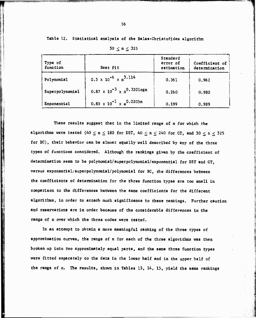
l^pppgpggjjg^ »■VJ..MMtfcy,W^^^^^

56

Table 12. Statistical analysis of the Balas-Christofides algorithm

50 < n < 325

Type of function Best fit

, 1

Standard error of estimation

! Coefficient of j determination

Polynomial

Superpolynomial

Exponential

0.5 x IQ'6 X n3'114

0.87 x 10"3 x n°-3201ogn

0.85 x 10"1 x e°-0205n

0.361

0.260

0.199

0.962 J

0.980

0.989

These results suggest that in the limited range of n for which the

algorithms were tested (40 < n < 180 for SST, 40 < n < 240 for CT, and 50 < n < 325

for BC), their behavior can be almost equally well described by any of the three

types of functions considered. Although the rankings given by the coefficient of

determination seem to be polynomial/superpolynomial/exponential for SST and CT,

versus exponential/superpolynomial/polynomial for BC, the differences between

the coefficients of determination for the three function types are too small in

comparison to the differences between the same coefficients for the different

algorithms, in order to attach much significance to these rankings. Further caution

and reservations are in order because of the considerable differences in the

range of n over which the three codes were tested.

In an attempt to obtain a more meaningful ranking of the three types of

approximation curves, the range of n for each of the three algorithms was then

broken up into two approximately equal parts, and the same three function types

were fitted separately to the data in the lower half and in the upper half of

the range of n. The results, shown in Tables 13, 14, 15, yield the same rankings

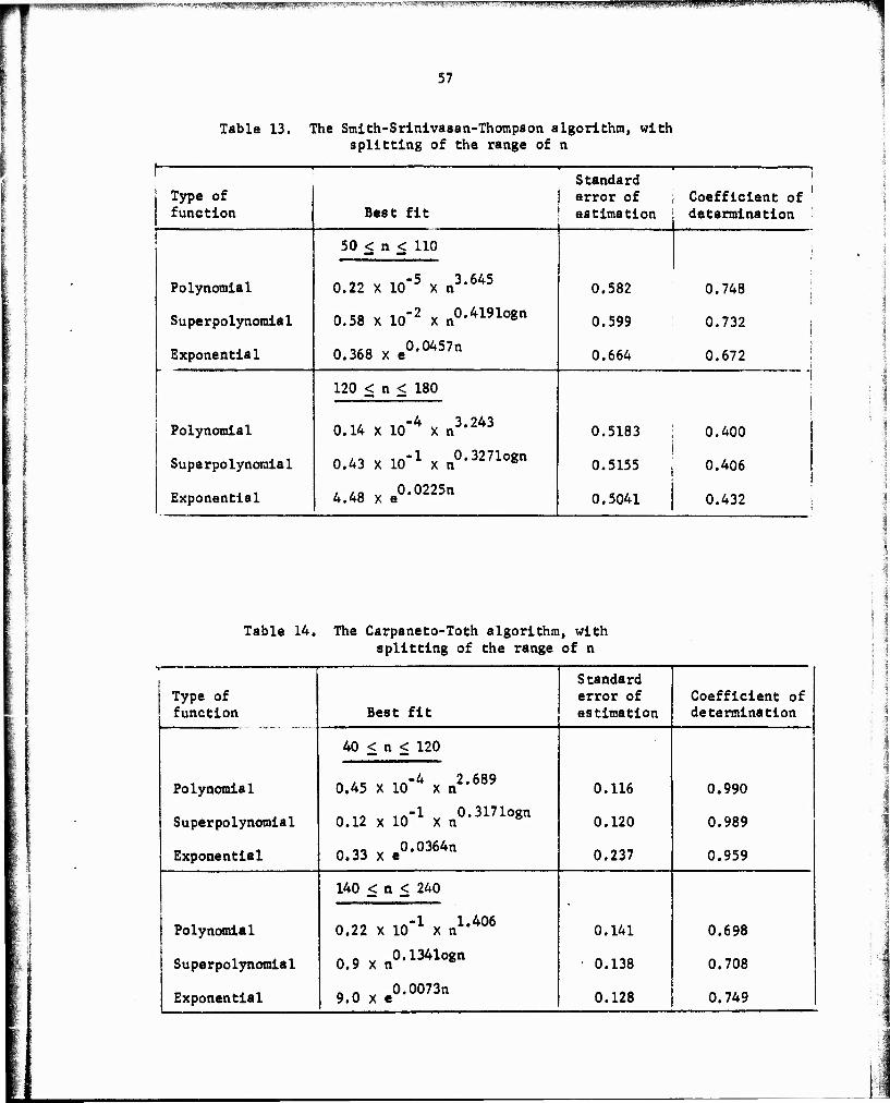
^i-^asMwiipui«^

57

Table 13. The Smith-Srinlvasan-Thompson algorithm, with splitting of the range of n

Type of function Best fit

Standard error of estimation

Coefficient of determination

50 < n < 110

0.582 Polynomial 0.22 x 10"5 x n3,645 0.748

Superpolynomial 0.58 X 10"2 x n°-4l91°8n 0.599 0.732

Exponential 0.368 x e°-0457n 0.664 0.672

120 < n < 180

Polynomial -4 3 243

0.14 X 10 X n '*** 0.5183 0.400

Superpolynomial 0.43 X IQ"1 X n°'3271°gn 0.5155 0.406

Exponential 4.48 x e°-0225n 0.5041 0.432

Table 14.

I I

The Carpaneto-Toth algorithm, with splitting of the range of n

Type of function Best fit

Standard error of estimation

Coefficient of determination

Polynomial

40 < n < 120

0.116 0.990 0.45 X IQ"4 x n2'689

Superpolynomial 0.12 xlO^xn0'317108" 0.120 0.989

Exponential 0.33 x e°-0364n 0.237 0.959

Polynomial

140 < n < 240

0.141 0.698 0.22 X 10"1 x n1'406

Superpolynomial 0.9 x n0'1341<*n 0.138 0.708

Exponential 9.0 x e°-0O73n 0.128 0.749

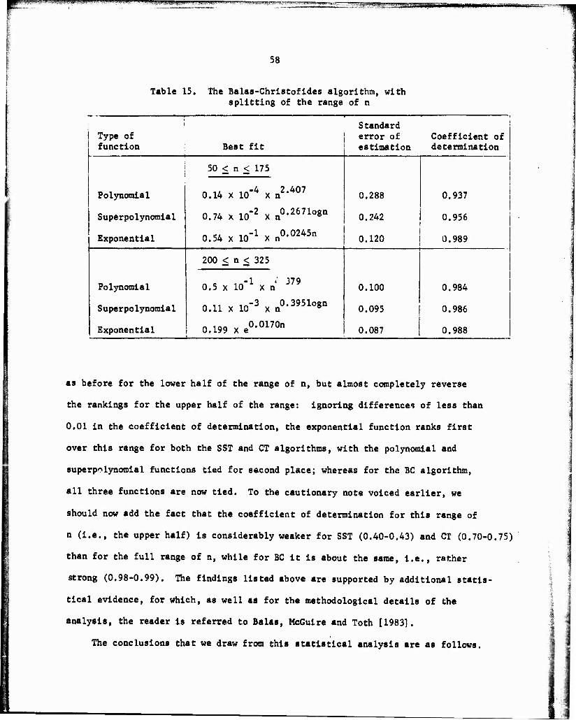
W§iffl^ffifl#jM*j^^ -*— --— 2^»iA!a35WiSfSng8B!i

58

Table 15. The Balas-Christofides algorithm, with splitting of the range of n

1

Type of function ! Best fit

Standard error of estimation

Coefficient of determination

Polynomial

50 < n < 175

0.288 0.937 0.14 x 10-4 X n2"407

Superpolynomial 0.74 X 10-2 X a0'2671o*n 0.242 0.956

Exponential 0.54 x lO"1 X n°'0245n 0.120 0.989

Polynomial

200 < n < 325

0.100 0.984 -1 '' 379

0.5 X 10 X n

Superpolynomial 0.11 X lO"3 X n°-3951°8n 0.095 0.986

Exponential 0.199 X e°-°170n 0.087 0.988

as before for the lower half of the range of n, but almost completely reverse

the rankings for the upper half of the range: ignoring differences of less than

0.01 in the coefficient of determination, the exponential function ranks first

over this range for both the SST and CT algorithms, with the polynomial and

superpolynomial functions tied for second place; whereas for the BC algorithm,

all three functions are now tied. To the cautionary note voiced earlier, we

should now add the fact that the coefficient of determination for this range of

n (i.e., the upper half) is considerably weaker for SST (0.40-0.43) and CT (0.70-0.75)

than for the full range of n, while for BC it is about the same, i.e., rather

strong (0.98-0.99). The findings listed above are supported by additional statis-

tical evidence, for which, as well as for the methodological details of the

analysis, the reader is referred to Balas, McGuire and Toth [1983].

The conclusions that we draw from this statistical analysis are as follows.

.■KBB^gggpag^paHgMpeggwm

59

First, over the limited range of a for which data are available, the per-

formance of the three algorithms analyzed can be described almost equally well

by each of the three function types considered: polynomial, superpolynomial and

exponential. Second, while the best fitting polynomial functions are of a moderate

degree (ranging between 1.4 and 4.4), the best fitting exponential functions have

a base very close to 1 (ranging between e * ■ 1.079 and e ' = 1.012). Note

that an exponential function of this type is very different from the function en.

While the value of the latter increases more than twice whenever the variable goes

from n to n + 1, the value of 1.012n increases only by 1.2 percent when the variable

goes from n to n + 1.

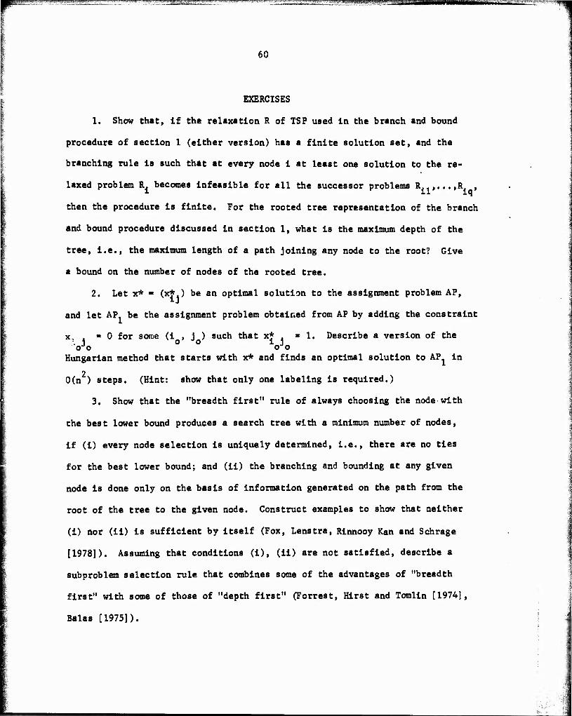
Ifssr* ^»"»^W-W^MIW."™—^ — '-—"-— ™™ —g'wr^TOagjgjgw^^s^M" - - - — "^^^^^^f^^

60

EXERCISES

1. Show that, if the relaxation R of TSP used in the branch and bound

procedure of section 1 (either version) has a finite solution set, and the

branching rule is such that at every node i at least one solution to the re-

laxed problem R. becomes infeasible for all the successor problems R..,...,R. ,

then the procedure is finite. For the rooted tree representation of the branch

and bound procedure discussed in section 1, what is the maximum depth of the

tree, i.e., the maximum length of a path joining any node to the root? Give

a bound on the number of nodes of the rooted tree.

2. Let x* = (x?,) be an optimal solution to the assignment problem AP,

and let AP be the assignment problem obtained from AP by adding the constraint

x. , = 0 for some (i , 1 ) such that x* ■ 1. Describe a version of the ■. 1 o o 11 oJo oJo

Hungarian method that starts with x* and finds an optimal solution to AP. in

2 0(n ) steps. (Hint: show that only one labeling is required.)

3. Show that the "breadth first" rule of always choosing the node with

the best lower bound produces a search tree with a minimum number of nodes,

if (i) every node selection is uniquely determined, i.e., there are no ties

for the best lower bound; and (ii) the branching and bounding at any given

node is done only on the basis of information generated on the path from the

root of the tree to the given node. Construct examples to show that neither

(i) nor (ii) is sufficient by itself (Fox, Lenstra, Rinnooy Kan and Schräge

[1978]). Assuming that conditions (i), (ii) are not satisfied, describe a

subproblem selection rule that combines some of the advantages of "breadth

first" with some of those of "depth first" (Forrest, Hirst and Tomlin [1974],

Balas [1975]).

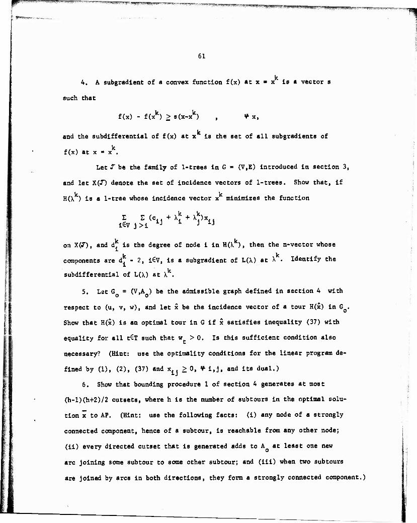
61

4. A subgradient of a convex function f(x) at x - x is a vector s

such that

f(x) - f(xk) > s(x-xk) , ¥• x,

and the subdifferential of f(x) at x is the set of all subgradients of

f(x) at x * x .

Let I be the family of 1-trees in G - (V,E) introduced in section 3,

and let X(J) denote the set of incidence vectors of 1-trees. Show that, if

k k H(X ) is a 1-tree whose incidence vector x minimizes the function

I I (c.. + Xk + \k)x.. i€v j>i lj * j 1J

k k on X(J"), and d is the degree of node i in H(\ ), then the n-vector whose

components are dk - 2, i€v, is a subgradient of L(\) at X . Identify the

subdifferential of L(\) at \k.

5. Let G ■ (V,A ) be the admissible graph defined in section 4 with

respect to (u, v, w), and let x be the incidence vector of a tour H(x) in G .

Show that H(x) is an optimal tour in G if x satisfies inequality (37) with

equality for all t<=T such that w > 0. Is this sufficient condition also

necessary? (Hint: use the optimality conditions for the linear program de-

fined by (1), (2), (37) and x±, > 0, ¥ i,j, and its dual.)

6. Show that bounding procedure 1 of section 4 generates at most

(h-l)(h+2)/2 cutsets, where h is the number of subtours in the optimal GOIU-

tion x to AP. (Hint: use the following facts: (i) any node of a strongly

connected component, hence of a subtour, is reachable from any other node;

(ii) every directed cutset that is generated adds to A at least one new

arc joining some subtour to some other subtour; and (iii) when two subtours

are joined by arcs in both directions, they form a strongly connected component.)

a» ,. 8»«'»P'''»»g*w*?ywgw^^

62

7. Show that, if B- is the lower bound on v(TSP) obtained by bounding

procedure 1, the lower bound generated by bounding procedure 2 is

2 l t€T2 *

(Hint: use the fact that if the cost of each arc in the set U (S , S ) t€T2

C

is increased by ^., then the value of the solution x (hence of the solution

(u,v) to the dual of AP obtained at the end of procedure 2) is v(AP) + I |S„in„.)

C2 t£T„' C C

8. Let k be an articulation point of the admissible graph G , let S be

the node set of one of the components of G -{k}, and consider the two directed

cutsets

K^ - (St, V\StU(k}), K^'- (V\StU0c}, Sfc}.

Show that the inequality

x, > 1 (i,J)€K^UKt

w j "

is the sum of the inequality (5) for S « S U {k}, the inequality (3) for S - St,

and the equations (2) for all i€S and j€St.

9. Formulate the n-path relaxation of the TSP discussed in section 5 for

both the asymmetric and the symmetric cases, with a Lagrangean function involving

the equations (2) (in the asymmetric case) or (7) (in the symmetric case). Give

some examples of side constraints, i.e., extra conditions, that this relaxation

of TSP can accommodate but the 1-arborescence or 1-tree relaxations can not. i ;>:

M

Vf$^w,,.,„

References

Agmon S., The relaxation method for linear inequalities. Canadian Journal of Mathematics. 6, 382-392, (1934).

Balas, E., Bivalent programming by implicit enumeration. In J. Beizer, A. G. Holzman and A. Kent (editors), Encyclopedia of Computer Science and Technology. Vol. 2, M. Dekker, New York, 479-494, (19/5).

Balas, E., Cutting planes from conditional bounds: a new approach to set covering. Mathematical Programming Study 12. 19-36, (1980).

3alas, E. and Christofides, N., A restricted Lagrangean approach to the traveling salesman problem. Mathematical Programming 21. 19-46, (1981).

Balas, E. and Guignard, M., Branch and bound/implicit enumeration. Annals of Discrete Mathematics 5. 185-191, (1979).

Balas, E., McGuire, T. W. and Toth, P., Statistical analysis of some traveling salesman algorithms. GSIA, Carnegie-Mellon University (1983).

Beale, E. M. L., Branch and bound methods for mathematical programming systems, Annals of Discrete Mathematics 5. 201-220, (1979).

3ellmore, M. and Malone, J.C., Pathology of traveling salesman subtour- elimination algorithms. Operations Research. 19, 278-307, (1971).

Carpaneto, G. and Toth, P., Some new branching and bounding criteria for the asymmetric travelling salesman problem. Management Science. 26, 736-743, (1980).

Christofides, N., "Graph Theory - An Algorithmic Approach," Academic Pres3, London, (1975).

Christofides, N., The shortest hamiltonian chain of a graph. J. SIAM (Applied Mathematics). 19, 689-696, (1970).

Christofides, N., The travelling salesman problem. In N. Christofides, A. Mingozzi, P. Toth and C. Sandi (editors), Combinatorial Optimization, J. Wiley, 131-149, (1979).

Christofides, N., Mingozzi, A. and Toth, P., State-Space relaxation procedures for the computation of bounds to routing problems. Networks, 11, 145-164, (1981).

Crowder, H. and Padberg, M.W., Solving large scale symmetric traveling salesman problems to optimality. Management Science. 26, 495-509 (1980).

Dantzig, G.B., Fulkerscn, D.R. and Johnson, S.U., Solution of a large traveling salesman problem, Operations Research. 2, 393-410, (1954).

Dantzig, G.3., Fulkerson, D.R. and Johnson, S.M., On a linear programming, combinatorial approach to the traveling salesman problem. Operations Research, 7, 58-66, (1959).

p»i™^m »™M^»^^ , i ,11 i .«■.i.ijll—liMm. ■ I IM ^'»■■■-"■■»■'KWWiiWiu.ia MMMBMBHHy^|

64

Dijkstra, E.K., A note on two problems in connection with graphs. Numerische Mathematik. 1, 269-271, (1959). ~

Eastman, W.L., Linear Programming with pattern constraints. Ph.D. Dissertation Harvard University, (1958). '

Edmonds, J., Optimum branchings. Journal of Research of the National Bureau of Standards. 71B. 233-240, (19677! ""

Fisher, M. L., The Lagrangean relaxation method for solving integer programming problems, Management Science. 27, 1-18, (1981).

Forrest, J. J. H., Hirst, J. P. H. and Tomlin, J. A., Practical solution of large and complex integer programming problems with UMPIRE. Management Science. 20, (1974). '"

Fox, B. L., Lenstra, J. K., Rinnooy Kan, A. H. G. and Schräge, L. E., Branching from the largest upper bound: folklore and facts. European Journal of Operational Research. 2, 191-194, (1978).

Fulkerson, D. R. , Packing rooted directed cuts in a weighted directed graph. Mathematical Programming, 6, 1-13, (1974).

Garfinkel, R. S. and Nemhauser, G. L., Integer programming. Wiley, (1972).

Geoffrion, A.M., Lagrangean relaxation and its uses in integer programming. Mstheiatical Programming Study 2. 82-114, (1974).

Gr'otschel, M. and Padberg, M.W., On the symmetric traveling salesman problem I: Inequalities, II: Lifting theorems and facets. Mathematical Programming. 16, 265-280 and 281-302, (1979).

Hall, M., Combinatorial Theory. Blaisdell Publishing Co., (1967).

Helbig Ksnsen, K. and Krarup, J., Improvements of the Held-Karp algorithm for the symmetric traveling-salesman problem. Mathematical programming. 4, 87-96, (1974).

Held, M. and Karp, R., The traveling-salesman problem and minimum spanning tree. Operations Research. 18, 1138-1162, (1970).

Held, M. and Karp, R., The traveling-salesman problem and minimum spanning tree: Part II. Mathematical Programming 1, 6-25, (1971).

Held, M., tfolfe, P. and Crowder, H.P., Validation of subgradient optimization, Mathematical Programming, 6, 62-88, (1974).

Houck, D., Picard, J.C., Queyranne, M. and Vemuganti, R.R., The traveling salesran problem and shortest n-paths., Teen. Rep. University of Maryland

(1977).

Kruskal, J.B., On the shortest spanning subtree of a graph and the traveling salesman problem. Proc. Amer. Math. Soc, 2, 48-50, (1956).

Kuhn, H. W., The Hungarian method for the assignment problem. Naval Research Logistics Quarterly. 2, 83-97, (1955).

-■:-:.■-— wvmwmmMW*"^'-»■■■'J4.ttMM^i»iw.iW»fHptWL_uu.,imiw'i'''™"''111»''- " ag---~-imiiTi»TiiiiTinii7iiiiiiTimTmr.'T^F?^^

65

Lawler, E. L., Combinatorial optimization: networks and matroids. Holt,

Rinehart and Winston, (1976).

Lenstra, J. K. and Rinnooy Kan, A. H. G., On the expected performance of branch and bound algorithms. Operations Research, 26, 347-350, (1978).

Little, J.D.C., Murty, J.G., Sweeney, D.W. and Karel, C, An algorithm for the traveling salesman problem. Operations Research. 11, 972-989, (1963).

Motzkin, T. and Schoenberg, I.J., The relaxation method for linear inequalities. Canadian Journal of Mathematics, 6, 393-404, (1954).

Murty, K., An algorithm for ranking all the assignments in order of increasing cost. Operations Research. 16, 682-687, (1968).

Polyak, B.T., A general method of solving extremum problems. Soviet Mathematics Doklady, 8, 593-597 (Translation of Doklady Akademii Nauk SSSR. 174). (1967).

Prim, R.C., Shortest connection networks and some generalizations. BSTJ, 36, 1389-1401, (1957).

Sandi, C., Subgradient -ptimization. In N. Christofides, A. Mingozzi, ?. Toth, and C. Sandi (editors), Combinatorial Optimization. J. Wiley, 73-91, (1979).

Shapiro, D.M., Algorithms for the solution of the optimal cost and bottleneck traveling salesman problems. Sc. D. Thesis, Washington university, St. Louis, (1966).

Shapiro, J.F., A survey of Lagrangean techniques for discrete optimization. Annals of Discrete Mathematics 5, 113-138, (1979).

Smith, T.H.C., A LIFO implicit enumeration algorithm for the asymmetric traveling salesman problem using a one-arborescence relaxation. Ph.D. Dissertation Chapter, Carnegie-Mellon University, Pittsburgh, (1975),

Smith, T.H.C. and Thompson, G.L., A LIFO Implicit enumeration search algorithm for the symmetric traveling salesman problem using Held and Karp's 1-tree relaxation. Annals of Discrete Mathematics, I. 479-493, (1977).

Smith, T.H.C., Srinivasan, V. and Thompson, G.L., Computational performance of three subtour elimination algorithms for solving asymmetric traveling salesman problems, Annals of Discrete Mathematics. 1, 495-506, (1977).

Spielberg, K., Enumerative methods in integer programming. Annals of Discrete Mathematics 5, 139-183, (1979).

Tarjan, R.E., Finding optimum branchings. Networks, 7, 25-35, (1977).

"olgenant, T. and Jonker, R...A branch and bound algorithm for the symmetric traveling salesman problem based on the 1-tree relaxation, European Journal of Operational Research. 9, 83-89, (1982).

^f^^j^m^m-.^^mi^^^ s^>fSB3ljiefK-44^ IPPM^ffllSISl^^ m i-. - -r -j PH

■•i,t •*■*> •*>•(• tfli»»»0

!CB* 5CCU«8fTA7ICN »AGE I ' «C?CB ' *.aie>

j MSRR 488

GCvT *CCtiIION nO.1 1. »«C'llHT'» C»~«wOG NUMJCK

Branch and Bound Methods for the Traveling Salesman Problem

». TV»C Or KCPOHT » HCaiOS COVERED

Technical Report March 1983

v PtnrotmHO one. *CPO«T «uuie«

, •■ CONT«ACJ OH C*A*f MUM8t»C(

j N00014-75-C-0621 ! NR 047-048 /

. Egon Balas and Paolo Toth

I

l. »IMO^MINO ORGANIZATION NAME «NO AOOKIU

Graduate School of Industrial Administration Carnegie-Mellon University Pittsburgh, PA 15213

10. »NOGaAM liLCMCNT. »J»«3JSCT. TASK >M* • WOMK UNIT NUMBERS

if. SS>.-«0.^.-«C Cf »I« *A«< AND «OOOCSS, „ Personnel and Training Research Programs Office of Nival Research (Code 434) Arlington, W 22217

'•♦ MONlTORlNO «OENCV NAME • Z55SGS(5 SMSMM B CMIMIIHII SiSS»

! IJ. o^o«? 0*T5

March 1983 is. NUMCC* or »Ases

65

!

: is. »ECURITY a.AS*, <••/ M» r^hMt;

' Unclassified

: 133! OSC^AS*l»ICATlC'i'J.-i».-^»«iHa i SCHEDULE

1 'S DlJTmft/T^ON STATEMENT •/ ••»»« *fH)

ffMs d"::

for py?- i

äiattibui!..:

- IINMMRfll ■'•voved

s- , '?. DISTRIBUTION STATEMENT (H Ittm **«»acr «H«M)MltoM 19. II ««MM «NN* ««■»>)

••. SUR»C«.MENTA*V NOT«

v 1*. KEY »OROS t&milmtm M nw» «M* M MMMT atf immMr *r MM* i

branch and bound, implicit enumeration, traveling salesman problem, combinatorial optimization, algorithm performance

I

J JO. ABSTRACT CCanflnu* m now«« «#«• If MMMT *** Hmtttf n »<•«* mm**) ( ] This paper reviews the state of the art in enumeratlve solution methods for thej j traveling salesman problem (TSP). The intröäuction (Section 1) discusses the j I main ingredients of branch and bound methods for the TSP. Sections 2, 3, and \ \ 4 discuss classes of methods based on three different relaxations of the TSP: * ] the assignment problem with the TSP cost function, the 1-tree problem with a J ] Lagrangean objective function, and the assignment problem with a Lagrangean J objective function. Section 5 briefly reviews some other relaxations of the j TSP, while Section 6 discusses the per feme nee of some state of the art

EDITION of i NOV •» ia oatottTt ... . (cont a) •"••«»•öl-««"' „CU..ITY ctssrifgffiaH^Sii rsss. v*z gs «..—>

DD , :sr*n 1473

... . ..«noum iMH.pi...M..j I..IJ.IIWI IUU jJHWPWVPf^n

computer codes. Besides material from the literature, the paper also includes the results and statistical analysis of some computational experiments designed for the purposes of this review.