CARe Seminar, NYCCARe Seminar, NYC

February 28, 2002February 28, 2002

Jonathan Hayes, ACAS, MAAAJonathan Hayes, ACAS, MAAA

Uncertainty AndUncertainty AndProperty Cat PricingProperty Cat Pricing

AgendaAgenda

ModelsModels Model ResultsModel Results Confidence BandsConfidence Bands

DataData Issues with DataIssues with Data Issues with InputsIssues with Inputs Model OutputsModel Outputs

Pricing MethodsPricing Methods Standard DeviationStandard Deviation Downside RiskDownside Risk

Role of JudgmentRole of Judgment Still NeededStill Needed

“A Nixon-Agnew administration will abolish the credibility gap and reestablish the truth – the whole truth – as its policy.”

Spiro T. Agnew, Sept. 21, 1973

The Search For TruthThe Search For Truth

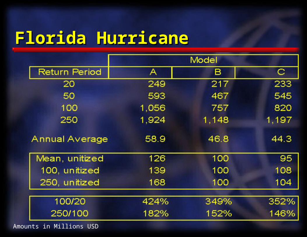
Florida HurricaneFlorida Hurricane

Amounts in Millions USD

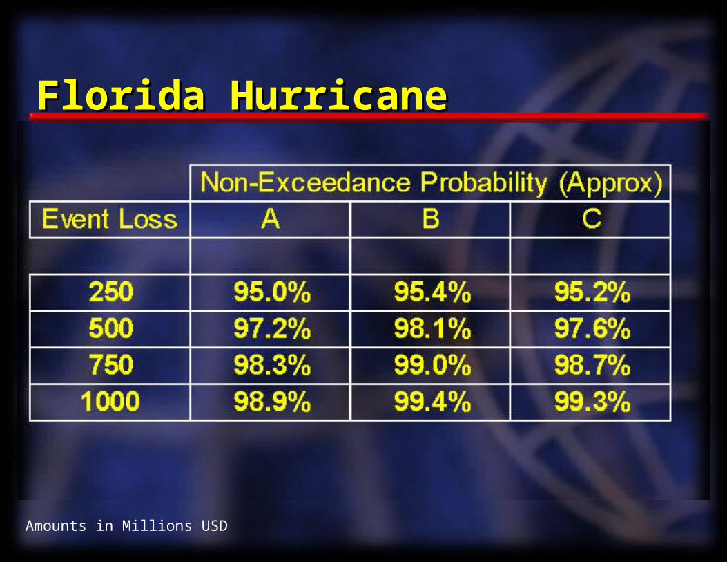
Florida HurricaneFlorida Hurricane

Amounts in Millions USD

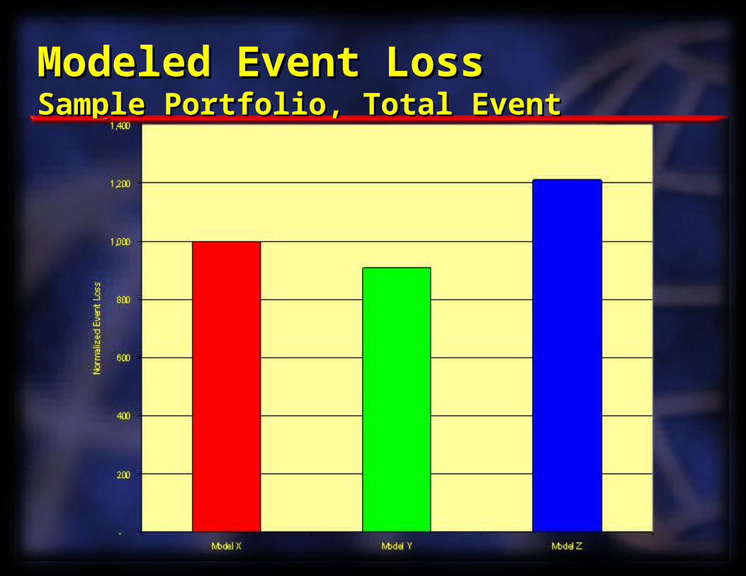
Modeled Event LossModeled Event LossSample Portfolio, Total EventSample Portfolio, Total Event

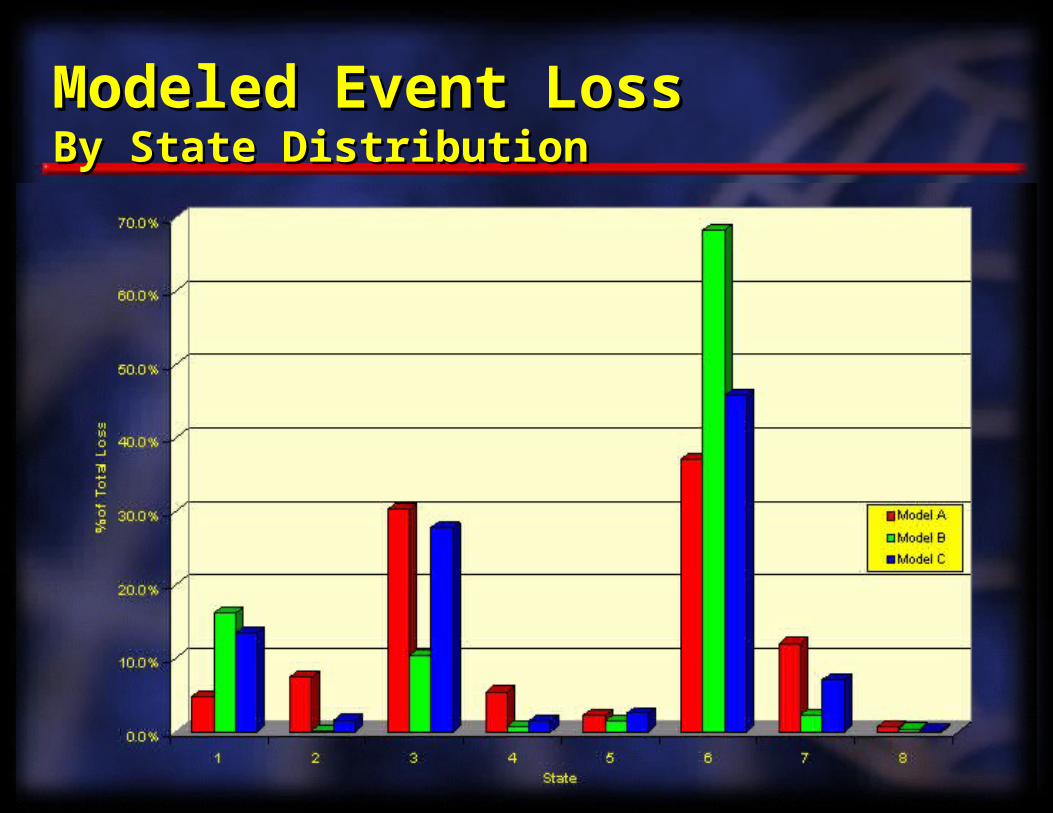
Modeled Event LossModeled Event LossBy State DistributionBy State Distribution

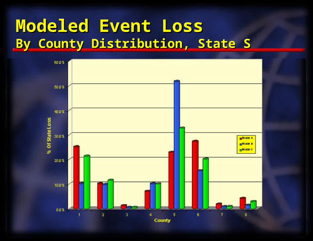
Modeled Event LossModeled Event LossBy County Distribution, State SBy County Distribution, State S

Why Don’t The Models Agree?Why Don’t The Models Agree?

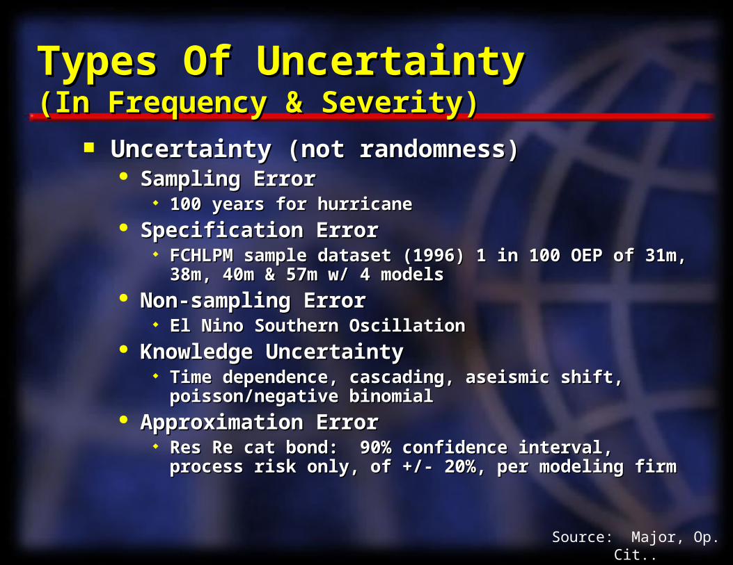
Types Of UncertaintyTypes Of Uncertainty(In Frequency & Severity)(In Frequency & Severity)

Uncertainty (not randomness)Uncertainty (not randomness) Sampling ErrorSampling Error

100 years for hurricane100 years for hurricane Specification ErrorSpecification Error

FCHLPM sample dataset (1996) 1 in 100 OEP of 31m, 38m, FCHLPM sample dataset (1996) 1 in 100 OEP of 31m, 38m, 40m & 57m w/ 4 models40m & 57m w/ 4 models

Non-sampling ErrorNon-sampling Error El Nino Southern OscillationEl Nino Southern Oscillation

Knowledge UncertaintyKnowledge Uncertainty Time dependence, cascading, aseismic shift, Time dependence, cascading, aseismic shift,

poisson/negative binomialpoisson/negative binomial Approximation ErrorApproximation Error

Res Re cat bond: 90% confidence interval, process risk Res Re cat bond: 90% confidence interval, process risk only, of +/- 20%, per modeling firmonly, of +/- 20%, per modeling firm

Source: Major, Op. Cit..

Frequency-Severity UncertaintyFrequency-Severity UncertaintyFrequency Uncertainty (Miller)Frequency Uncertainty (Miller)

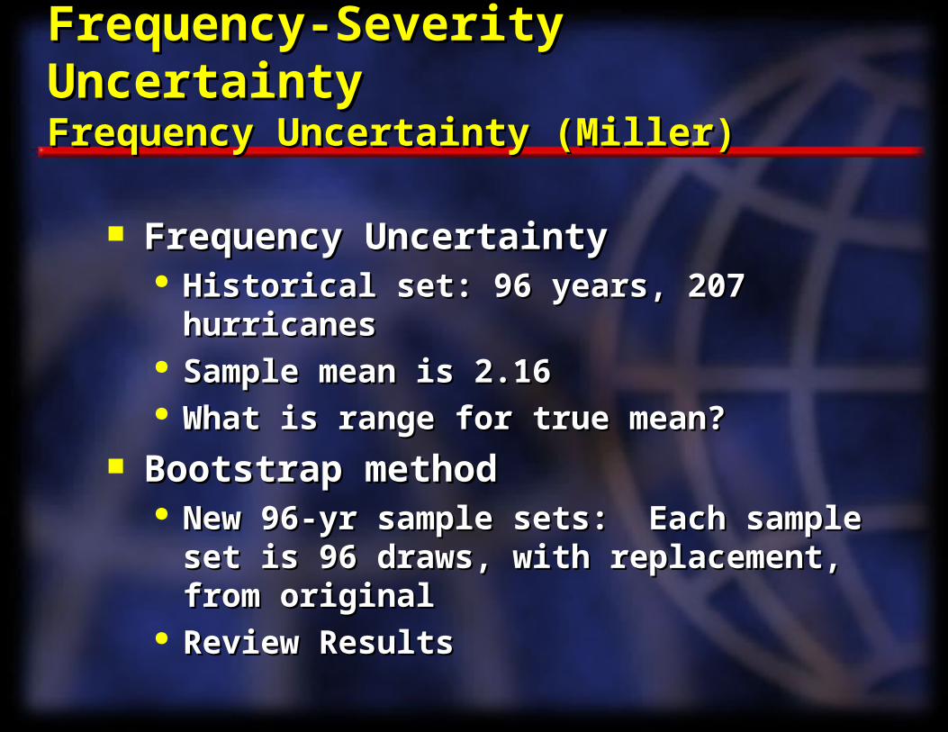
Frequency UncertaintyFrequency Uncertainty Historical set: 96 years, 207 hurricanesHistorical set: 96 years, 207 hurricanes Sample mean is 2.16Sample mean is 2.16 What is range for true mean?What is range for true mean?

Bootstrap methodBootstrap method New 96-yr sample sets: Each sample set New 96-yr sample sets: Each sample set

is 96 draws, with replacement, from is 96 draws, with replacement, from originaloriginal

Review ResultsReview Results

Frequency BootstrappingFrequency Bootstrapping Run 500 resamplings and graph relative Run 500 resamplings and graph relative

to theoretical t-distributionto theoretical t-distribution

Source: Miller, Op. Cit.

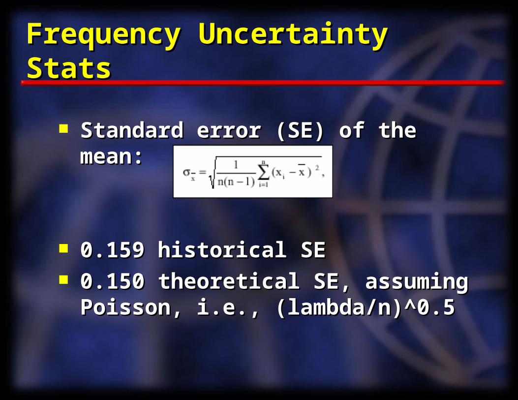
Frequency Uncertainty StatsFrequency Uncertainty Stats

Standard error (SE) of the mean:Standard error (SE) of the mean:

0.159 historical SE 0.159 historical SE 0.150 theoretical SE, assuming 0.150 theoretical SE, assuming

Poisson, i.e., (lambda/n)^0.5Poisson, i.e., (lambda/n)^0.5

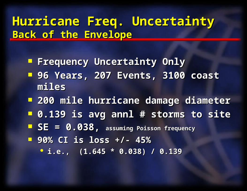
Hurricane Freq. UncertaintyHurricane Freq. UncertaintyBack of the EnvelopeBack of the Envelope

Frequency Uncertainty OnlyFrequency Uncertainty Only 96 Years, 207 Events, 3100 coast miles96 Years, 207 Events, 3100 coast miles 200 mile hurricane damage diameter200 mile hurricane damage diameter 0.139 is avg annl # storms to site0.139 is avg annl # storms to site SE = 0.038, SE = 0.038, assuming Poisson frequencyassuming Poisson frequency

90% CI is loss +/- 45%90% CI is loss +/- 45% i.e., (1.645 * 0.038) / 0.139i.e., (1.645 * 0.038) / 0.139

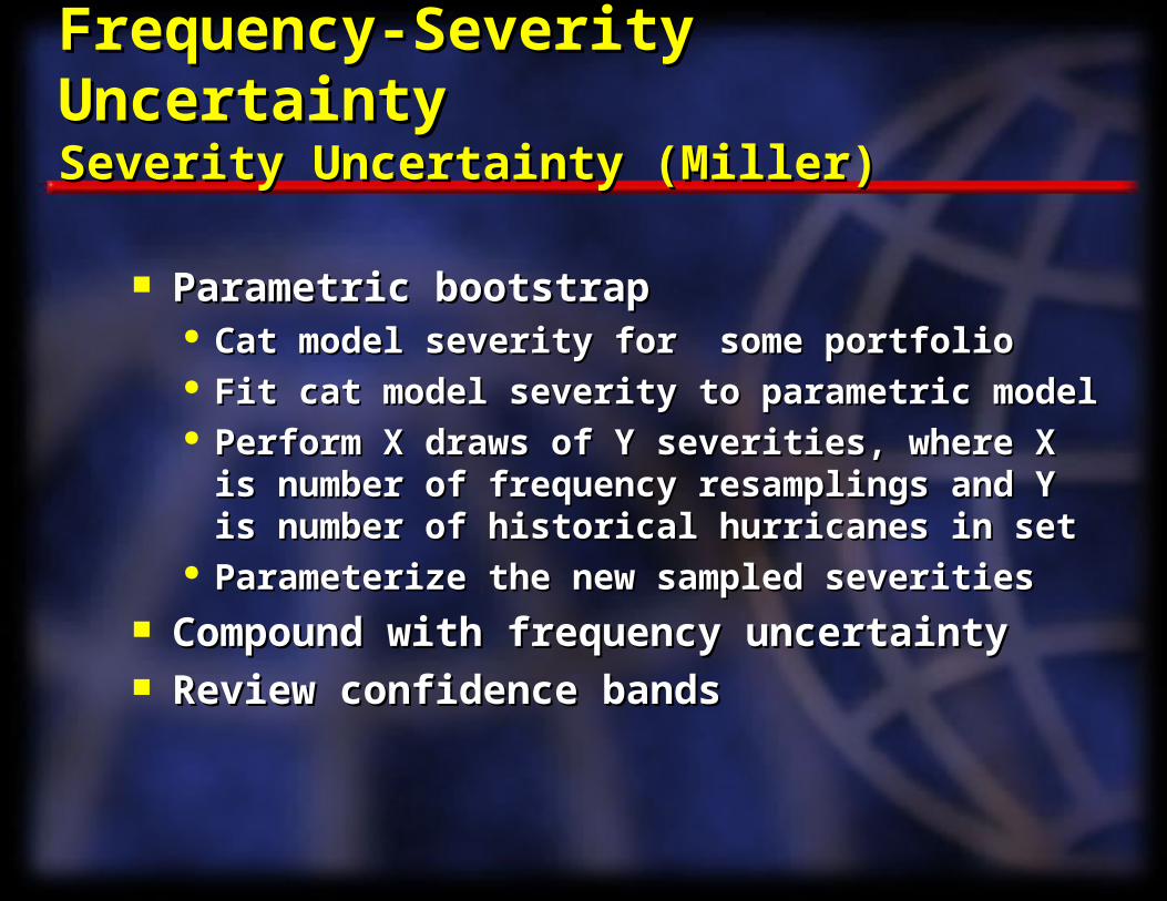
Frequency-Severity UncertaintyFrequency-Severity UncertaintySeverity Uncertainty (Miller)Severity Uncertainty (Miller)

Parametric bootstrapParametric bootstrap Cat model severity for some portfolio Cat model severity for some portfolio Fit cat model severity to parametric modelFit cat model severity to parametric model Perform X draws of Y severities, where X Perform X draws of Y severities, where X

is number of frequency resamplings and Y is number of frequency resamplings and Y is number of historical hurricanes in setis number of historical hurricanes in set

Parameterize the new sampled severitiesParameterize the new sampled severities Compound with frequency uncertaintyCompound with frequency uncertainty Review confidence bandsReview confidence bands

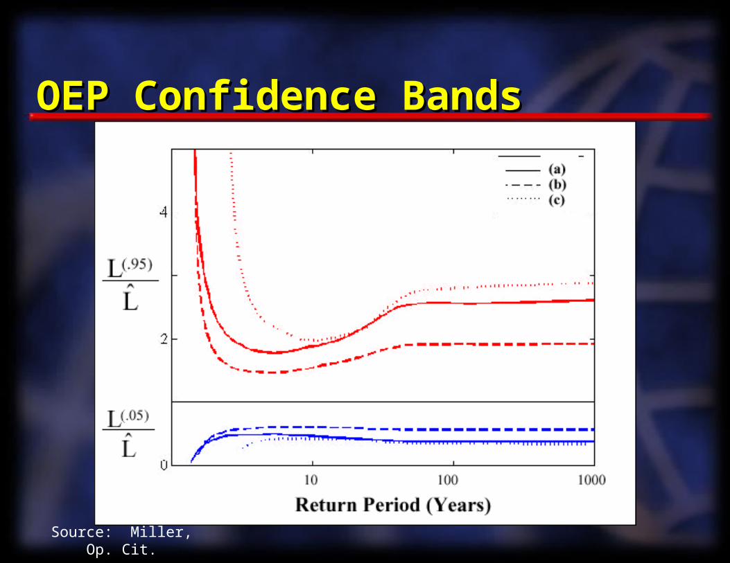
OEP Confidence BandsOEP Confidence Bands

Source: Miller, Op. Cit.

OEP Confidence BandsOEP Confidence Bands

Source: Miller, Op. Cit.

Model 1 in 50 1 in 100 1 in 250

A 127 139 168B 100 100 100C 117 104 108

FL HURRICANE EXAMPLE, REVISITED

OEP Confidence BandsOEP Confidence Bands

At 80-1,000 year return, range fixes to 50% to At 80-1,000 year return, range fixes to 50% to 250% of best estimate OEP250% of best estimate OEP

Confidence band grow exponentially at Confidence band grow exponentially at frequent OEP points because expected loss frequent OEP points because expected loss goes to zerogoes to zero

NotesNotes Assumed stationary climateAssumed stationary climate Severity parameterization may introduce errorSeverity parameterization may introduce error Modelers’ “secondary uncertainty” may overlap Modelers’ “secondary uncertainty” may overlap

here, thus reducing rangehere, thus reducing range Modelers’ severity distributions based on more Modelers’ severity distributions based on more

than just historical data setthan just historical data set

The Building BlocksThe Building BlocksPolicy Records/TIVPolicy Records/TIV

Data Collection/InputsData Collection/Inputs Is this all the subject data?Is this all the subject data?

All/coastal statesAll/coastal states Inland Marine, Builders Risk, APD, Dwelling FireInland Marine, Builders Risk, APD, Dwelling Fire Manual policiesManual policies

General level of detailGeneral level of detail County/zip/streetCounty/zip/street Aggregated dataAggregated data

Is this all the needed policy detail?Is this all the needed policy detail? Building location/billing locationBuilding location/billing location Multi-location policies/bulk dataMulti-location policies/bulk data Statistical Record vs. policy systemsStatistical Record vs. policy systems Coding of endorsementsCoding of endorsements

Sublimits, wind exclusions, IMSublimits, wind exclusions, IM Replacement cost vs. limitReplacement cost vs. limit

More Data IssuesMore Data Issues

Deductible issuesDeductible issues Inuring/facultative reinsuranceInuring/facultative reinsurance Extrapolations & DefaultsExtrapolations & Defaults Blanket policiesBlanket policies HPRHPR Excess policiesExcess policies

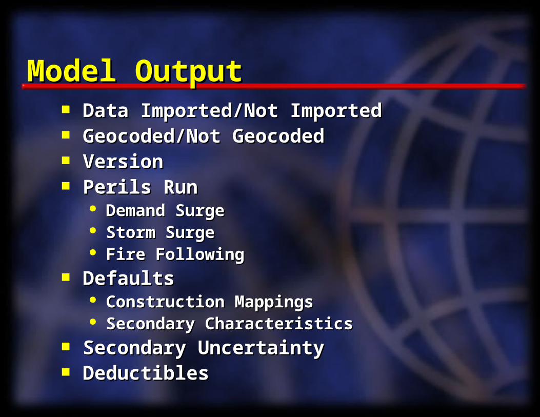
Model OutputModel Output Data Imported/Not ImportedData Imported/Not Imported Geocoded/Not GeocodedGeocoded/Not Geocoded VersionVersion Perils RunPerils Run

Demand SurgeDemand Surge Storm SurgeStorm Surge Fire FollowingFire Following

DefaultsDefaults Construction MappingsConstruction Mappings Secondary CharacteristicsSecondary Characteristics

Secondary UncertaintySecondary Uncertainty DeductiblesDeductibles

Synthesis/PricingSynthesis/Pricing

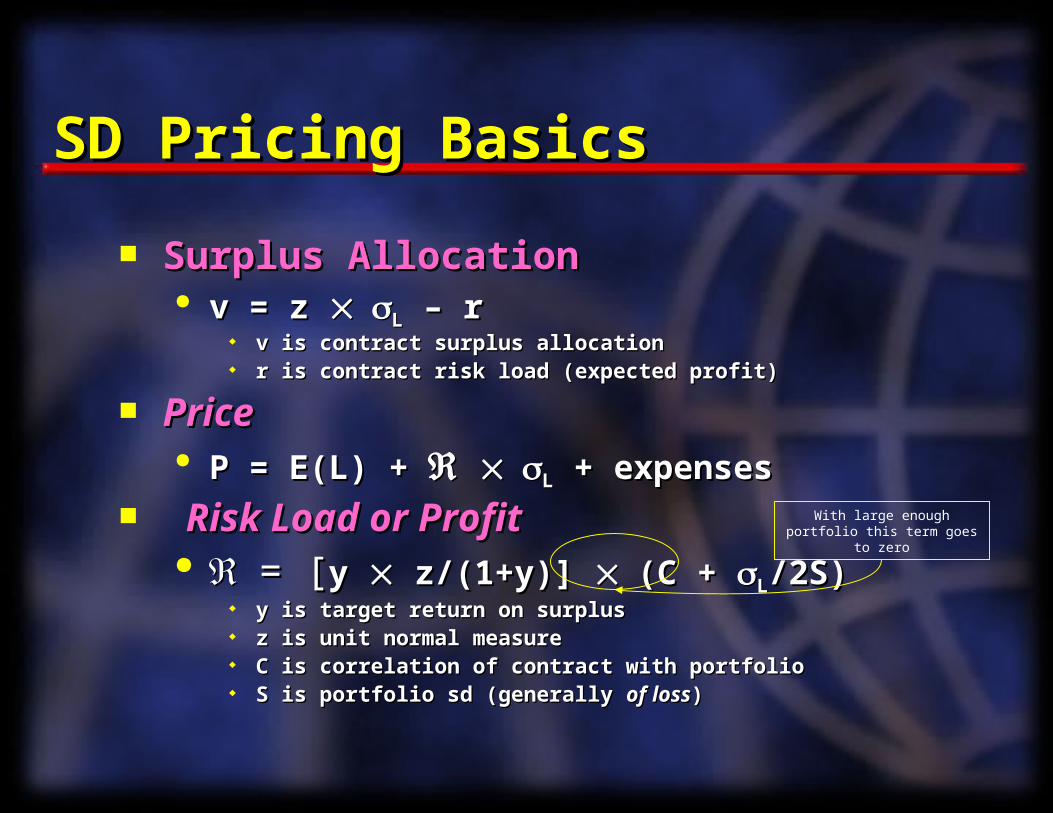
SD Pricing BasicsSD Pricing Basics

Surplus AllocationSurplus Allocation v = z v = z LL – r – r

v is contract surplus allocationv is contract surplus allocation r is contract risk load (expected profit)r is contract risk load (expected profit)

PricePrice P = E(L) + P = E(L) + LL + expenses + expenses

Risk Load or ProfitRisk Load or Profit = [= [y y z/(1+y)] z/(1+y)] (C + (C + LL/2S)/2S)

y is target return on surplusy is target return on surplus z is unit normal measurez is unit normal measure C is correlation of contract with portfolioC is correlation of contract with portfolio S is portfolio sd (generally S is portfolio sd (generally of lossof loss))

With large enough portfolio this term goes to zero

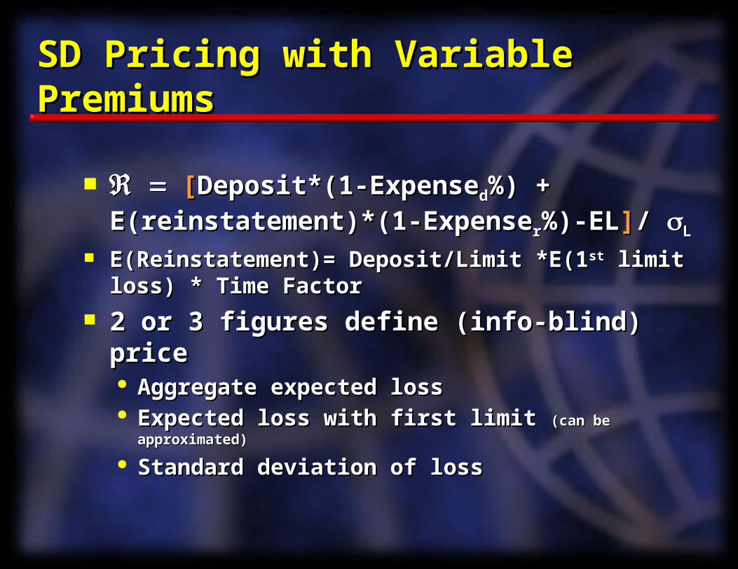
SD Pricing with Variable PremiumsSD Pricing with Variable Premiums

[[Deposit*(1-ExpenseDeposit*(1-Expensedd%) + %) +

E(reinstatement)*(1-ExpenseE(reinstatement)*(1-Expenserr%)-EL%)-EL]]/ / LL

E(Reinstatement)= Deposit/Limit *E(1E(Reinstatement)= Deposit/Limit *E(1stst limit limit loss) * Time Factorloss) * Time Factor

2 or 3 figures define (info-blind) price2 or 3 figures define (info-blind) price Aggregate expected lossAggregate expected loss Expected loss with first limitExpected loss with first limit (can be approximated)(can be approximated)

Standard deviation of lossStandard deviation of loss

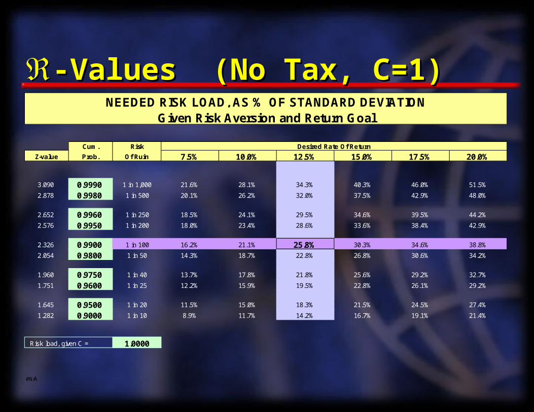
-Values (No Tax, C=1)-Values (No Tax, C=1)

Cum. Risk

Z-value Prob. Of Ruin 7.5% 10.0% 12.5% 15.0% 17.5% 20.0%

3.090 0.9990 1 in 1,000 21.6% 28.1% 34.3% 40.3% 46.0% 51.5%

2.878 0.9980 1 in 500 20.1% 26.2% 32.0% 37.5% 42.9% 48.0%

2.652 0.9960 1 in 250 18.5% 24.1% 29.5% 34.6% 39.5% 44.2%

2.576 0.9950 1 in 200 18.0% 23.4% 28.6% 33.6% 38.4% 42.9%

2.326 0.9900 1 in 100 16.2% 21.1% 25.8% 30.3% 34.6% 38.8%

2.054 0.9800 1 in 50 14.3% 18.7% 22.8% 26.8% 30.6% 34.2%

1.960 0.9750 1 in 40 13.7% 17.8% 21.8% 25.6% 29.2% 32.7%

1.751 0.9600 1 in 25 12.2% 15.9% 19.5% 22.8% 26.1% 29.2%

1.645 0.9500 1 in 20 11.5% 15.0% 18.3% 21.5% 24.5% 27.4%

1.282 0.9000 1 in 10 8.9% 11.7% 14.2% 16.7% 19.1% 21.4%

Risk load, given C = 1.0000

#N/A

Desired Rate Of Return

NEEDED RISK LOAD, AS % OF STANDARD DEVIATIONGiven Risk Aversion and Return Goal

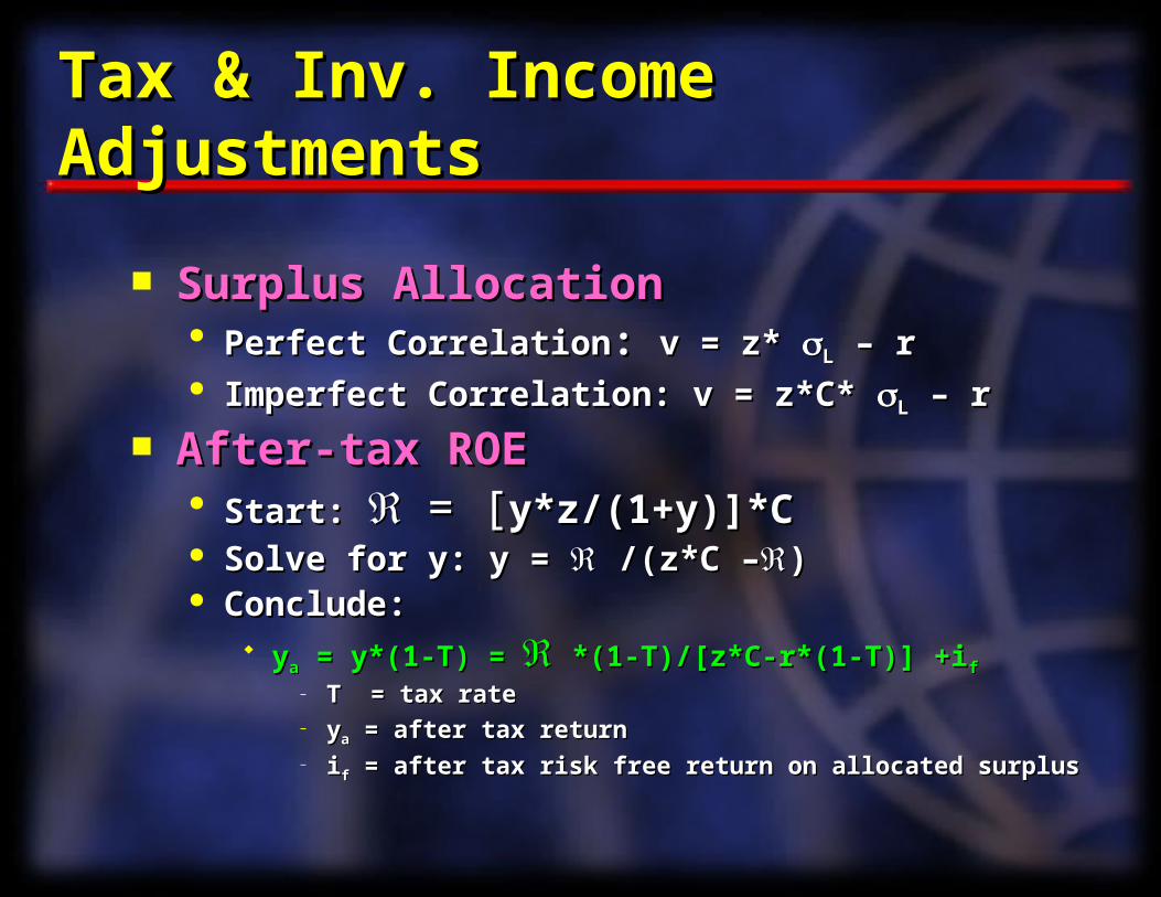
Tax & Inv. Income AdjustmentsTax & Inv. Income Adjustments

Surplus AllocationSurplus Allocation Perfect CorrelationPerfect Correlation: : v = z* v = z* LL – r – r Imperfect Correlation: v = z*C* Imperfect Correlation: v = z*C* LL – r – r

After-tax ROEAfter-tax ROE Start:Start:= [= [y*z/(1+y)]*Cy*z/(1+y)]*C Solve for y: y = Solve for y: y = /(z*C – /(z*C –)) Conclude:Conclude:

yyaa = y*(1-T) = = y*(1-T) = *(1-T)/[z*C-r*(1-T)] +i *(1-T)/[z*C-r*(1-T)] +iff

– T = tax rateT = tax rate– yyaa = after tax return = after tax return– iiff = after tax risk free return on allocated surplus = after tax risk free return on allocated surplus

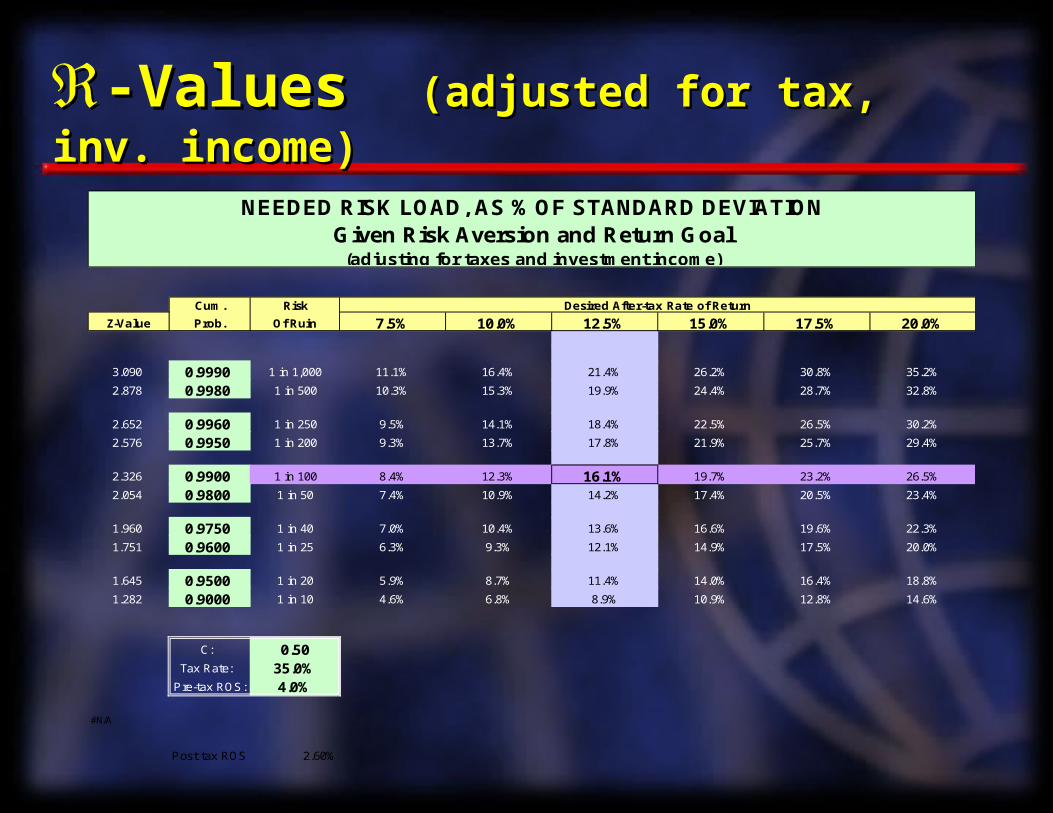
-Values -Values (adjusted for tax, inv. income)(adjusted for tax, inv. income)

Cum. Risk

Z-Value Prob. Of Ruin 7.5% 10.0% 12.5% 15.0% 17.5% 20.0%

3.090 0.9990 1 in 1,000 11.1% 16.4% 21.4% 26.2% 30.8% 35.2%

2.878 0.9980 1 in 500 10.3% 15.3% 19.9% 24.4% 28.7% 32.8%

2.652 0.9960 1 in 250 9.5% 14.1% 18.4% 22.5% 26.5% 30.2%

2.576 0.9950 1 in 200 9.3% 13.7% 17.8% 21.9% 25.7% 29.4%

2.326 0.9900 1 in 100 8.4% 12.3% 16.1% 19.7% 23.2% 26.5%

2.054 0.9800 1 in 50 7.4% 10.9% 14.2% 17.4% 20.5% 23.4%

1.960 0.9750 1 in 40 7.0% 10.4% 13.6% 16.6% 19.6% 22.3%

1.751 0.9600 1 in 25 6.3% 9.3% 12.1% 14.9% 17.5% 20.0%

1.645 0.9500 1 in 20 5.9% 8.7% 11.4% 14.0% 16.4% 18.8%

1.282 0.9000 1 in 10 4.6% 6.8% 8.9% 10.9% 12.8% 14.6%

C: 0.50Tax Rate: 35.0%

Pre-tax ROS: 4.0%

#N/A

Post tax ROS 2.60%

NEEDED RISK LOAD, AS % OF STANDARD DEVIATION

(adjusting for taxes and investment income)

Desired After-tax Rate of Return

Given Risk Aversion and Return Goal

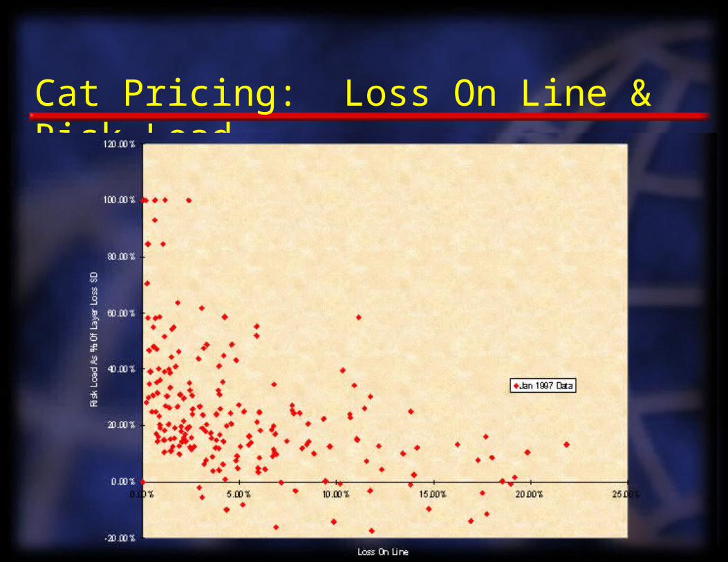
Cat Pricing: Loss On Line & Risk Load

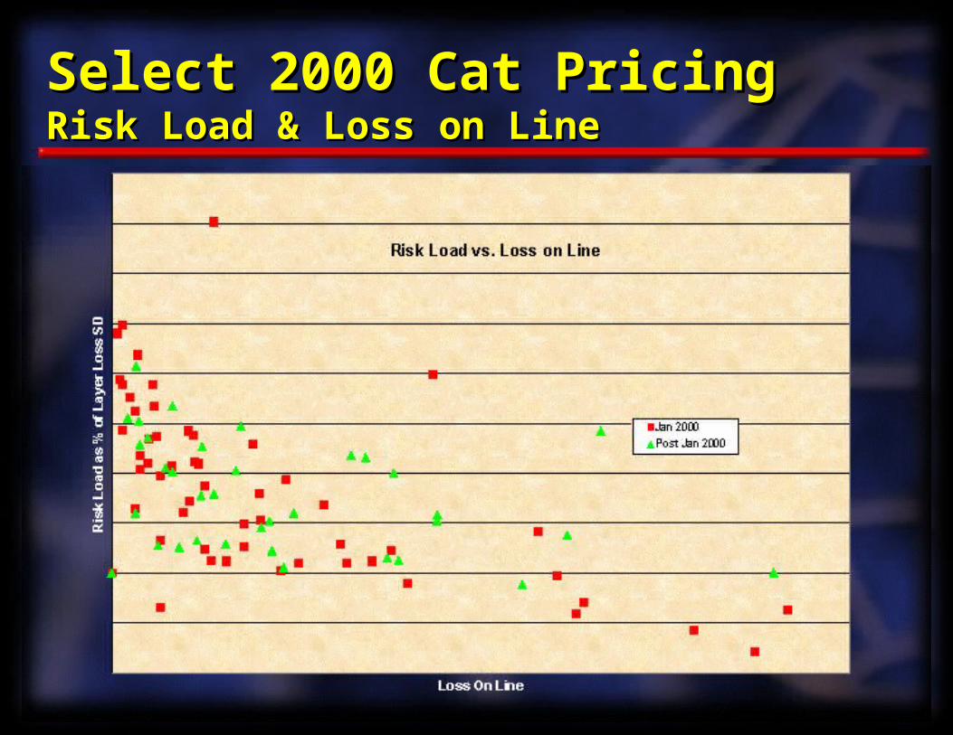
Select 2000 Cat PricingSelect 2000 Cat PricingRisk Load & Loss on LineRisk Load & Loss on Line

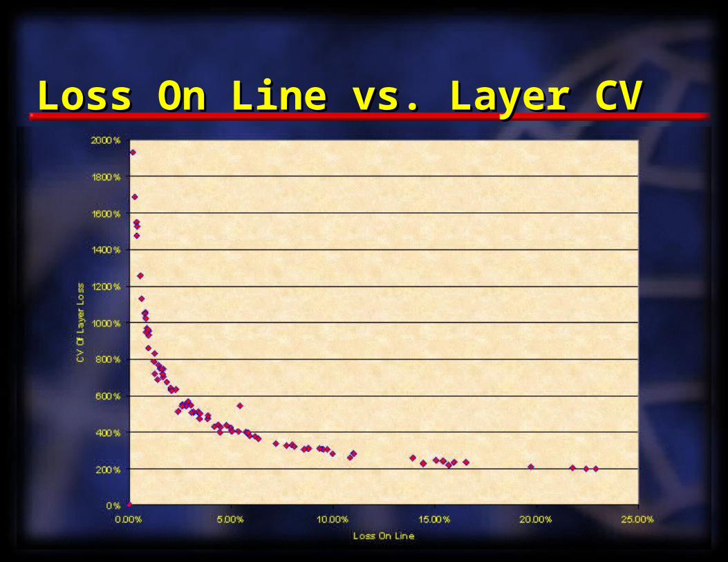
Loss On Line vs. Layer CVLoss On Line vs. Layer CV

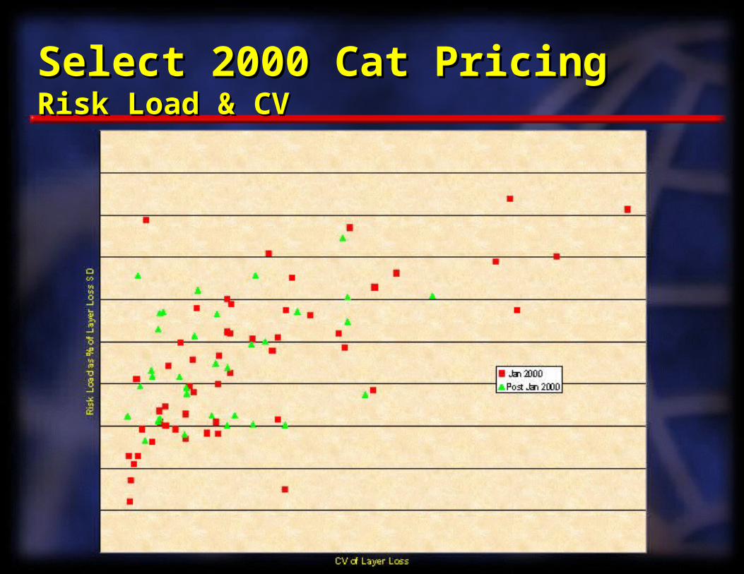
Select 2000 Cat PricingSelect 2000 Cat PricingRisk Load & CVRisk Load & CV

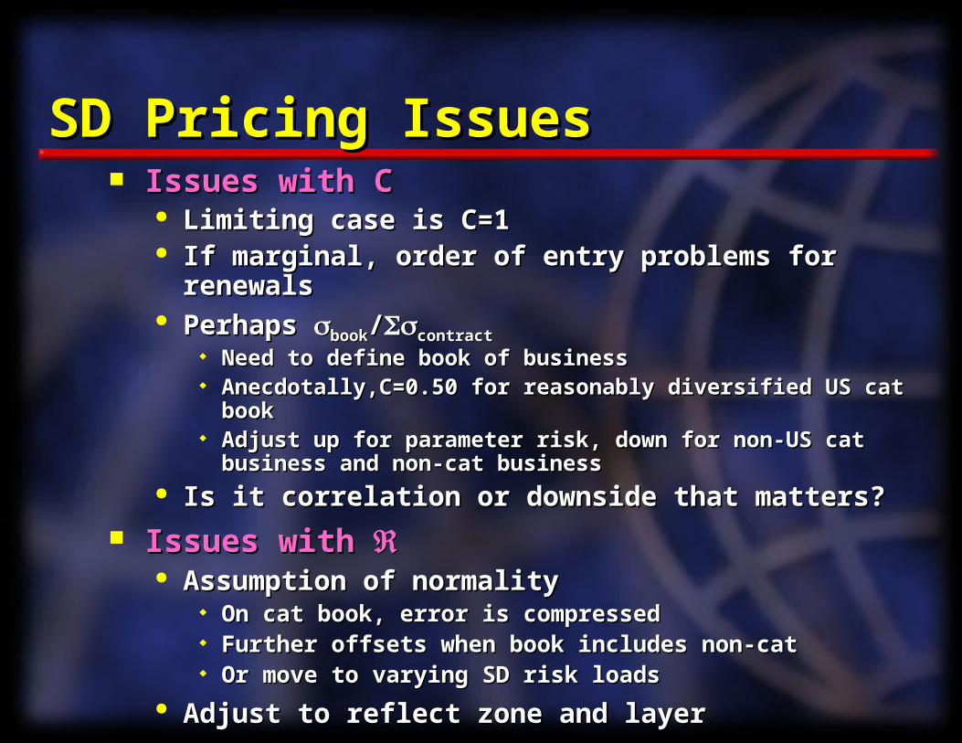
SD Pricing IssuesSD Pricing Issues Issues with CIssues with C

Limiting case is C=1Limiting case is C=1 If marginal, order of entry problems for renewalsIf marginal, order of entry problems for renewals Perhaps Perhaps bookbook//contractcontract

Need to define book of businessNeed to define book of business Anecdotally,C=0.50 for reasonably diversified US cat bookAnecdotally,C=0.50 for reasonably diversified US cat book Adjust up for parameter risk, down for non-US cat Adjust up for parameter risk, down for non-US cat

business and non-cat businessbusiness and non-cat business Is it correlation or downside that matters?Is it correlation or downside that matters?

Issues with Issues with Assumption of normalityAssumption of normality

On cat book, error is compressedOn cat book, error is compressed Further offsets when book includes non-catFurther offsets when book includes non-cat Or move to varying SD risk loadsOr move to varying SD risk loads

Adjust to reflect zone and layerAdjust to reflect zone and layer

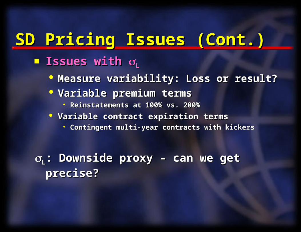
SD Pricing Issues (Cont.)SD Pricing Issues (Cont.) Issues with Issues with LL

Measure variability: Loss or result?Measure variability: Loss or result? Variable premium termsVariable premium terms

Reinstatements at 100% vs. 200%Reinstatements at 100% vs. 200% Variable contract expiration termsVariable contract expiration terms

Contingent multi-year contracts with kickersContingent multi-year contracts with kickers

LL: Downside proxy – can we get precise?: Downside proxy – can we get precise?

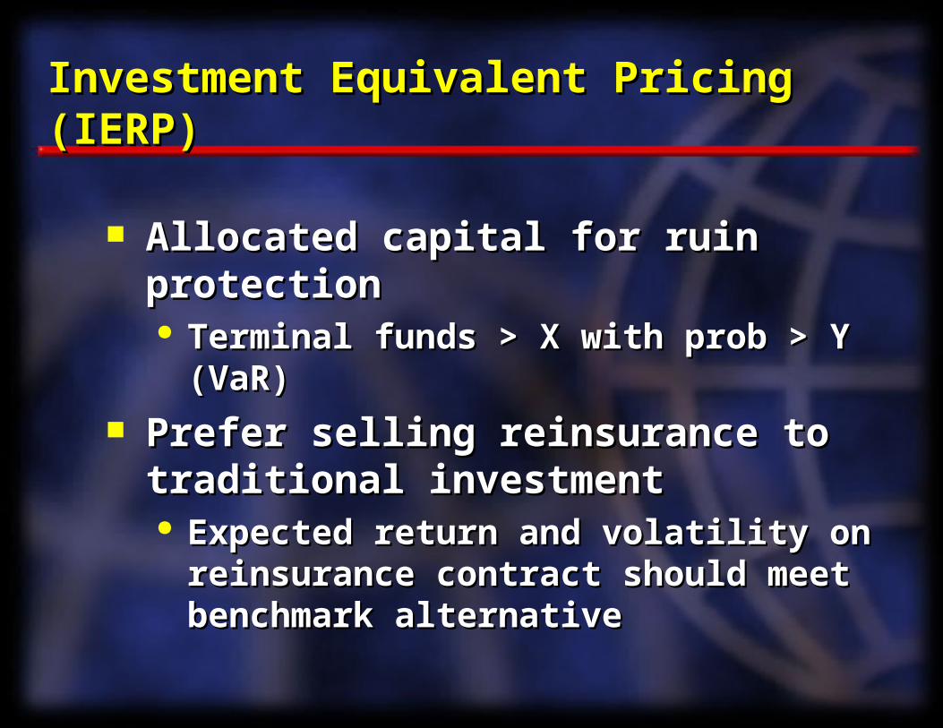
Investment Equivalent Pricing (IERP)Investment Equivalent Pricing (IERP)

Allocated capital for ruin protectionAllocated capital for ruin protection Terminal funds > X with prob > Y (VaR) Terminal funds > X with prob > Y (VaR)

Prefer selling reinsurance to traditional Prefer selling reinsurance to traditional investmentinvestment Expected return and volatility on Expected return and volatility on

reinsurance contract should meet reinsurance contract should meet benchmark alternativebenchmark alternative

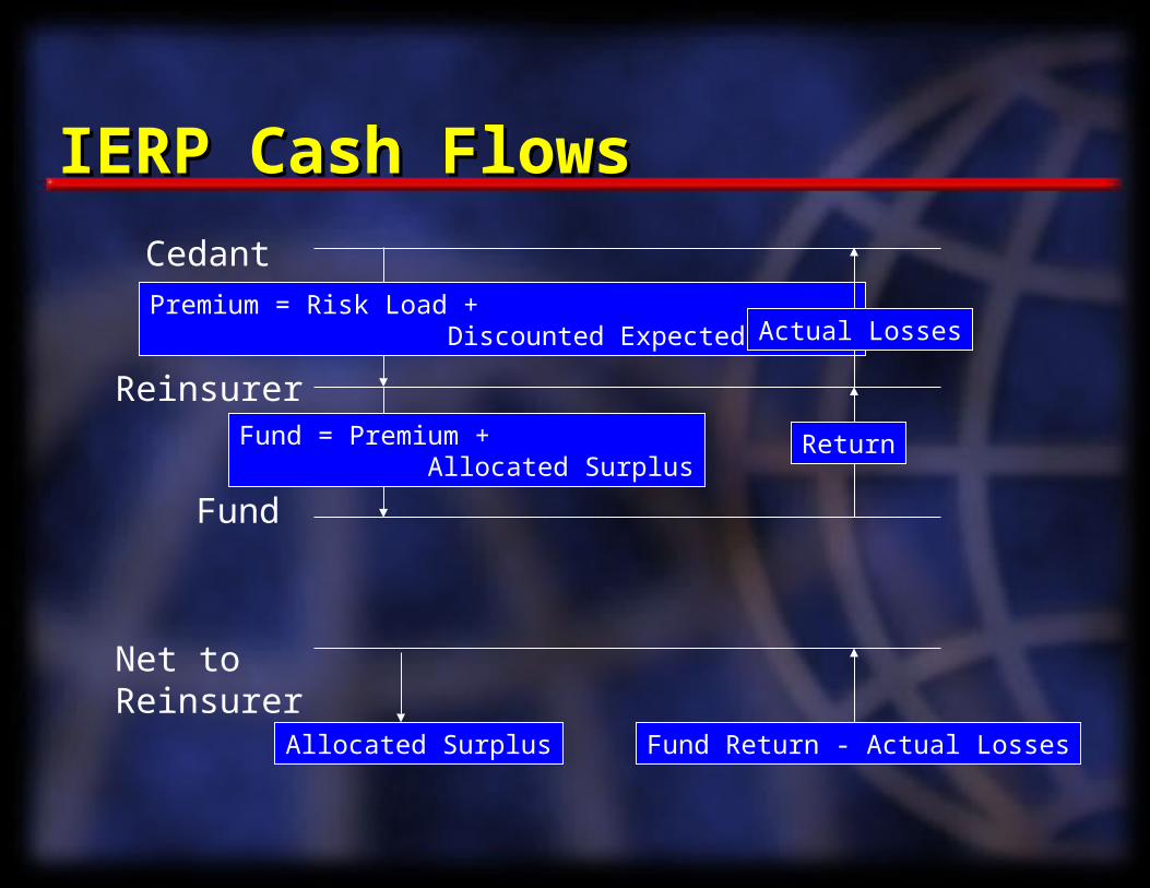
IERP Cash FlowsIERP Cash Flows

Cedant

Reinsurer

Fund

Premium = Risk Load + Discounted Expected Losses

Fund = Premium + Allocated Surplus

Return

Actual Losses

Net to Reinsurer

Allocated Surplus Fund Return - Actual Losses

IERP - Fully Funded VersionIERP - Fully Funded Version

Cedant

Reinsurer

Fund

P = R + E[]/(1+f)

F = P + A (1+rf)F

Expected return criterion: (1+rf)F - E[] = (1+y)A

Variance criterion: Var[] < y2A2

Safety criterion: (1+rf)F > S

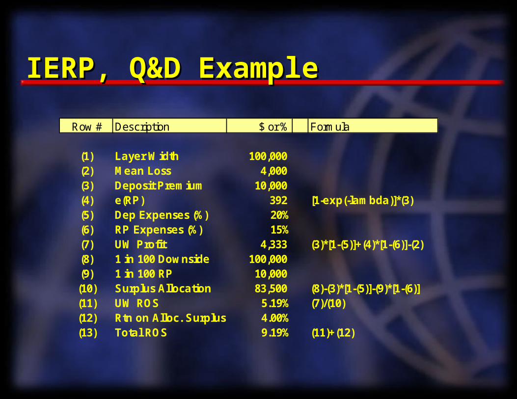
IERP, Q&D ExampleIERP, Q&D Example

Row # Description $ or % Formula

(1) Layer Width 100,000 (2) Mean Loss 4,000 (3) Deposit Premium 10,000 (4) e(RP) 392 [1-exp(-lambda)]*(3)(5) Dep Expenses (%) 20%(6) RP Expenses (%) 15%(7) UW Profit 4,333 (3)*[1-(5)]+(4)*[1-(6)]-(2)(8) 1 in 100 Downside 100,000 (9) 1 in 100 RP 10,000 (10) Surplus Allocation 83,500 (8)-(3)*[1-(5)]-(9)*[1-(6)](11) UW ROS 5.19% (7)/(10)(12) Rtn on Alloc. Surplus 4.00%(13) Total ROS 9.19% (11)+(12)

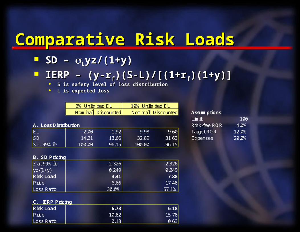
Comparative Risk LoadsComparative Risk Loads SD – SD – LLyz/(1+y)yz/(1+y) IERP – (y-rIERP – (y-rff)(S-L)/[(1+r)(S-L)/[(1+rff)(1+y)])(1+y)]

S is safety level of loss distributionS is safety level of loss distribution L is expected lossL is expected loss

Nominal Discounted Nominal Discounted AssumptionsLimit 100

A. Loss Distribution Risk-free ROR 4.0%EL 2.00 1.92 9.98 9.60 Target ROR 12.0%SD 14.21 13.66 32.89 31.63 Expenses 20.0%S = 99%ile 100.00 96.15 100.00 96.15

B. SD PricingZ at 99%ile 2.326 2.326yz/(1+y) 0.249 0.249Risk Load 3.41 7.88Price 6.66 17.48Loss Ratio 30.0% 57.1%

C. IERP PricingRisk Load 6.73 6.18Price 10.82 15.78Loss Ratio 0.18 0.63

2% Unlimited EL 10% Unlimited EL

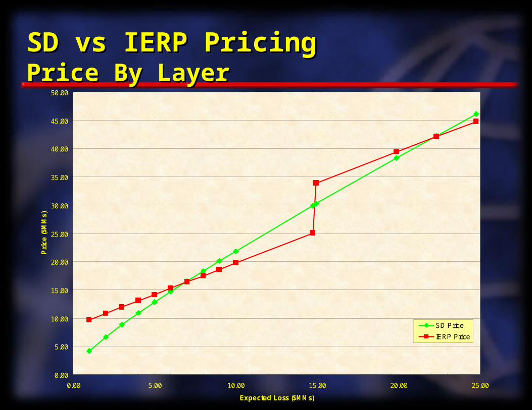
0.00

5.00

10.00

15.00

20.00

25.00

30.00

35.00

40.00

45.00

50.00

0.00 5.00 10.00 15.00 20.00 25.00

Expected Loss ($MMs)

Pri

ce (

$MM

s)

SD Price

IERP Price

SD vs IERP PricingSD vs IERP PricingPrice By LayerPrice By Layer

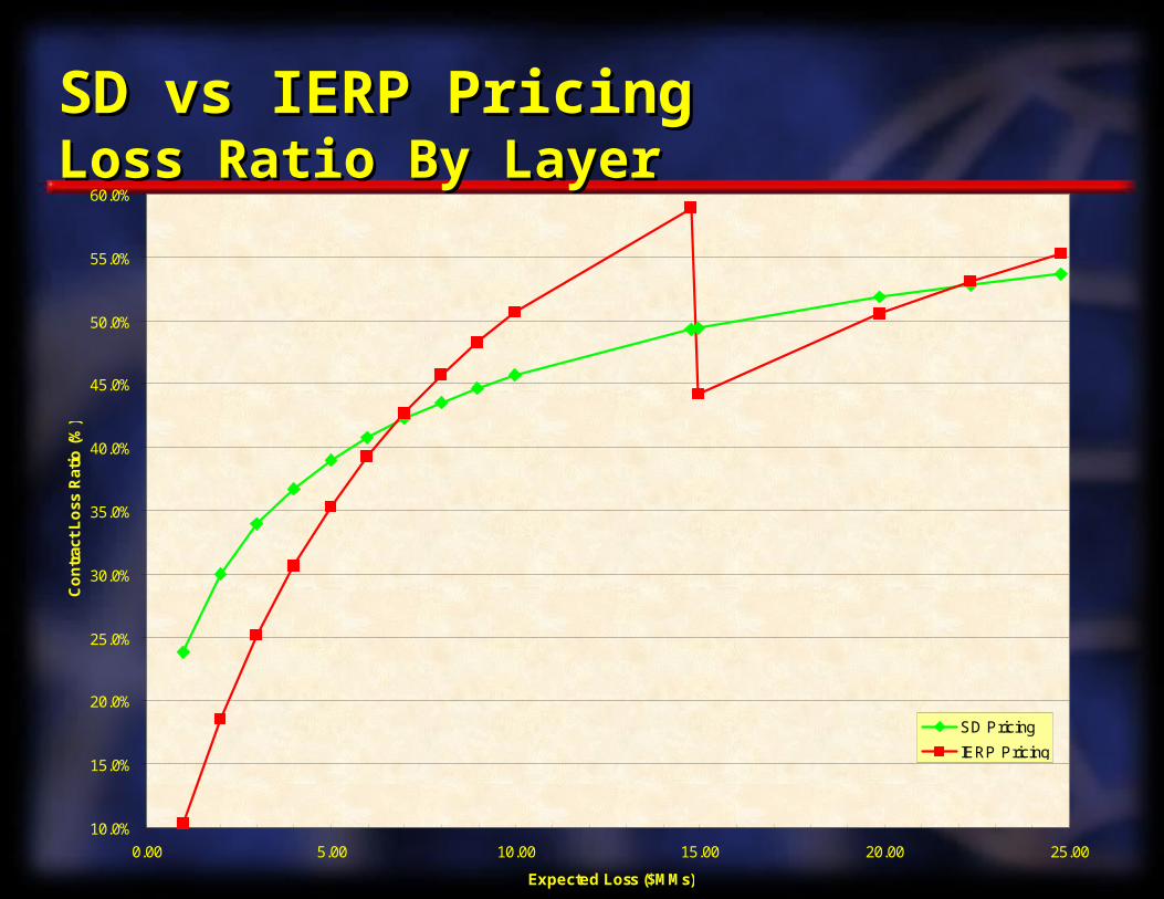
10.0%

15.0%

20.0%

25.0%

30.0%

35.0%

40.0%

45.0%

50.0%

55.0%

60.0%

0.00 5.00 10.00 15.00 20.00 25.00

Expected Loss ($MMs)

Co

ntr

act

Lo

ss R

atio

(%

)

SD Pricing

IERP Pricing

SD vs IERP PricingSD vs IERP PricingLoss Ratio By LayerLoss Ratio By Layer

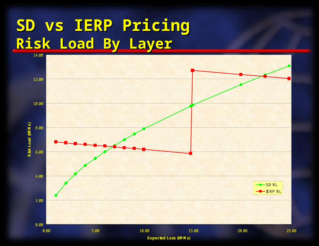
0.00

2.00

4.00

6.00

8.00

10.00

12.00

14.00

0.00 5.00 10.00 15.00 20.00 25.00

Expected Loss ($MMs)

Ris

k L

oad

($M

Ms)

SD RL

IERP RL

SD vs IERP PricingSD vs IERP PricingRisk Load By LayerRisk Load By Layer

ConclusionsConclusions

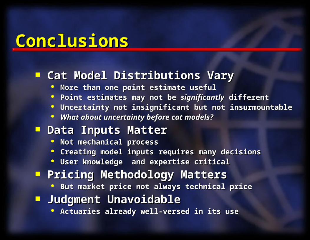
Cat Model Distributions VaryCat Model Distributions Vary More than one point estimate usefulMore than one point estimate useful Point estimates may not be Point estimates may not be significantlysignificantly different different Uncertainty not insignificant but not insurmountableUncertainty not insignificant but not insurmountable What about uncertainty before cat models?What about uncertainty before cat models?

Data Inputs MatterData Inputs Matter Not mechanical processNot mechanical process Creating model inputs requires many decisionsCreating model inputs requires many decisions User knowledge and expertise criticalUser knowledge and expertise critical

Pricing Methodology MattersPricing Methodology Matters But market price not always technical priceBut market price not always technical price

Judgment UnavoidableJudgment Unavoidable Actuaries already well-versed in its useActuaries already well-versed in its use

ReferencesReferences Bove, Mark C. et al.., “Effect of El Nino on US Landfalling Hurricanes, Bove, Mark C. et al.., “Effect of El Nino on US Landfalling Hurricanes,

Revisited,”Revisited,” Bulletin of the American Meteorological Society Bulletin of the American Meteorological Society , June 1998., June 1998. Efron, Bradley and Robert Tibshirani, Efron, Bradley and Robert Tibshirani, An Introduction to the BootstrapAn Introduction to the Bootstrap, ,

New York: Chapman & Hall, 1993.New York: Chapman & Hall, 1993. Kreps, Rodney E., “Risk Loads from Marginal Surplus Requirements,” Kreps, Rodney E., “Risk Loads from Marginal Surplus Requirements,”

PCAS LXXVIIPCAS LXXVII, 1990., 1990. Kreps, Rodney E., “Investment-equivalent Risk Pricing,” Kreps, Rodney E., “Investment-equivalent Risk Pricing,” PCAS LXXXVPCAS LXXXV, ,

1998. 1998. Major, John A., “Uncertainty in Catastrophe Models,” Major, John A., “Uncertainty in Catastrophe Models,” Financing Risk Financing Risk

and Reinsuranceand Reinsurance, International Risk Management Institute, Feb/Mar , International Risk Management Institute, Feb/Mar 1999.1999.

Mango, Donald F., “Application of Game Theory: Property Catastrophe Mango, Donald F., “Application of Game Theory: Property Catastrophe Risk Load,” Risk Load,” PCAS LXXXVPCAS LXXXV, 1998., 1998.

Miller, David, “Uncertainty in Hurricane Risk Modeling and Miller, David, “Uncertainty in Hurricane Risk Modeling and Implications for Securitization,” Implications for Securitization,” CAS Forum,CAS Forum, Spring 1999. Spring 1999.

Moore, James F., “Tail Estimation and Catastrophe Security Pricing: Moore, James F., “Tail Estimation and Catastrophe Security Pricing: Cat We Tell What Target We Hit If We Are Shooting in the Dark”, Cat We Tell What Target We Hit If We Are Shooting in the Dark”, Wharton Financial Institutions CenterWharton Financial Institutions Center, 99-14., 99-14.

Q&AQ&A

APPENDIX ASTANDARD DEVIATION PRICING

Derivation Of Formulas

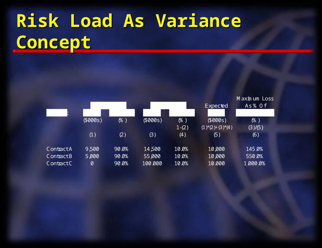
Risk Load As Variance ConceptRisk Load As Variance Concept

Maximum Loss Outcome 1 Outcome 2 Expected As % Of

Contract Loss Probability Loss Probability Value Expected Value($000s) (%) ($000s) (%) ($000s) (%)

1-(2) (1)*(2)+(3)*(4) (3)/(5)(1) (2) (3) (4) (5) (6)

Contract A 9,500 90.0% 14,500 10.0% 10,000 145.0%Contract B 5,000 90.0% 55,000 10.0% 10,000 550.0%Contract C 0 90.0% 100,000 10.0% 10,000 1,000.0%

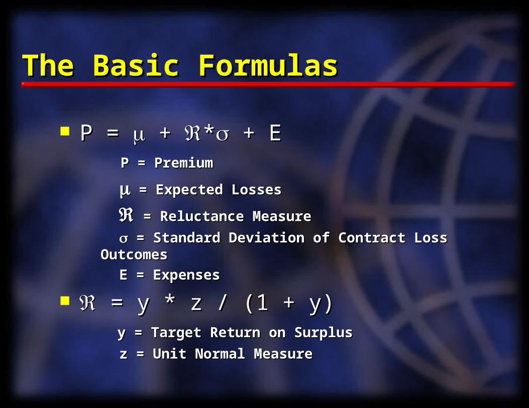
The Basic FormulasThe Basic Formulas

P = P = + + ** + E + E P = Premium P = Premium

= Expected Losses= Expected Losses

= Reluctance Measure= Reluctance Measure

= Standard Deviation of Contract Loss Outcomes= Standard Deviation of Contract Loss Outcomes

E = ExpensesE = Expenses

= y * z / (1 + y)= y * z / (1 + y) y = Target Return on Surplusy = Target Return on Surplus

z = Unit Normal Measurez = Unit Normal Measure

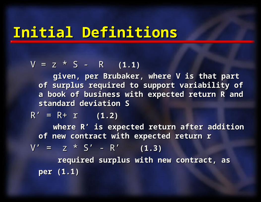
Initial DefinitionsInitial Definitions

V = z * S - V = z * S - RR (1.1) (1.1)

given, per Brubaker, where V is that part of surplus given, per Brubaker, where V is that part of surplus required to support variability of a book of business required to support variability of a book of business with expected return R and standard deviation S with expected return R and standard deviation S

R’ = R+ rR’ = R+ r (1.2) (1.2)

where R’ is expected return after addition of new where R’ is expected return after addition of new contract with expected return rcontract with expected return r

V’ = z * S’ - R’V’ = z * S’ - R’ (1.3) (1.3)

required surplus with new contract, as per (1.1)required surplus with new contract, as per (1.1)

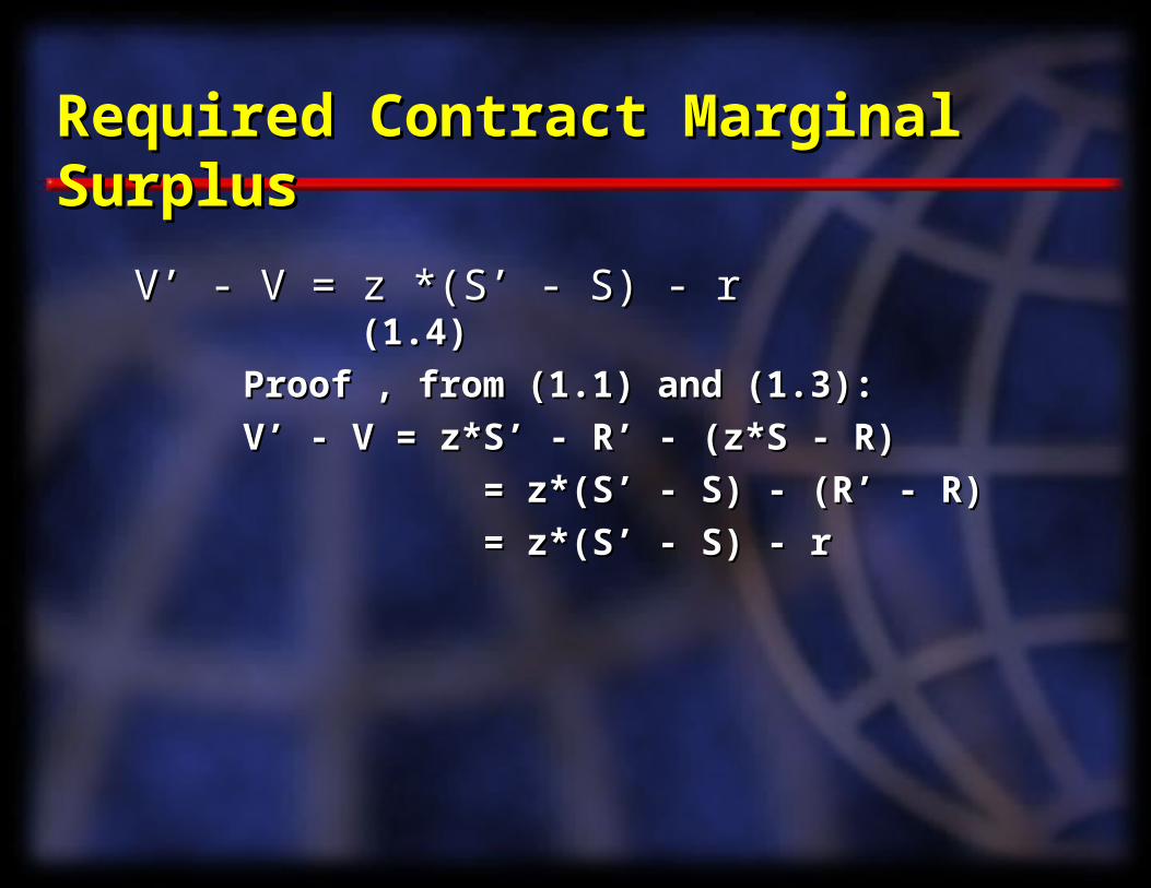
Required Contract Marginal SurplusRequired Contract Marginal Surplus

V’ - V = z *(S’ - S) - rV’ - V = z *(S’ - S) - r (1.4) (1.4)

Proof , from (1.1) and (1.3):Proof , from (1.1) and (1.3):

V’ - V = z*S’ - R’ - (z*S - R)V’ - V = z*S’ - R’ - (z*S - R)

= z*(S’ - S) - (R’ - R)= z*(S’ - S) - (R’ - R)

= z*(S’ - S) - r = z*(S’ - S) - r

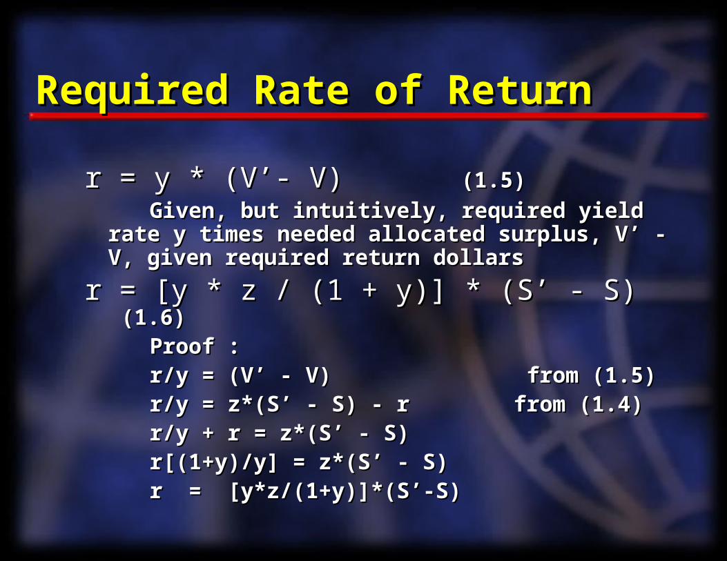
Required Rate of ReturnRequired Rate of Return

r = y * (V’- V)r = y * (V’- V) (1.5) (1.5)

Given, but intuitively, required yield rate y times Given, but intuitively, required yield rate y times needed allocated surplus, V’ - V, given required needed allocated surplus, V’ - V, given required return dollarsreturn dollars

r = [y * z / (1 + y)] * (S’ - S)r = [y * z / (1 + y)] * (S’ - S) (1.6) (1.6)

Proof :Proof : r/y = (V’ - V) from (1.5)r/y = (V’ - V) from (1.5) r/y = z*(S’ - S) - r from (1.4) r/y = z*(S’ - S) - r from (1.4) r/y + r = z*(S’ - S) r/y + r = z*(S’ - S) r[(1+y)/y] = z*(S’ - S)r[(1+y)/y] = z*(S’ - S) r = [y*z/(1+y)]*(S’-S)r = [y*z/(1+y)]*(S’-S)

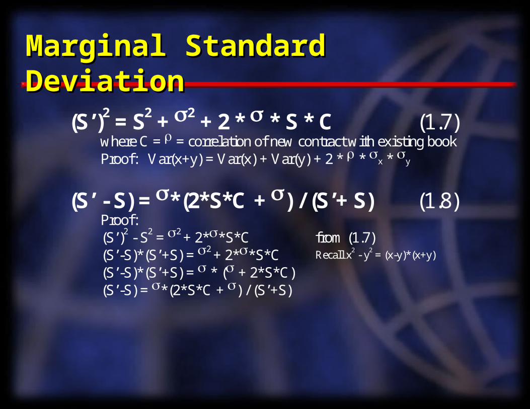
Marginal Standard DeviationMarginal Standard Deviation

(S’)2 = S2 + 2 + 2 * * S * C (1.7) where C = = correlation of new contract with existing book Proof: Var(x+y) = Var(x) + Var(y) + 2 * * x * y

(S’ - S) = *(2*S*C + ) / (S’+ S) (1.8) Proof:

(S’)2 - S2 = 2 + 2**S*C from (1.7)(S’-S)*(S’+S) = 2 + 2**S*C Recall x2 - y2 = (x-y)*(x+y)

(S’-S)*(S’+S) = * ( + 2*S*C)(S’-S) = *(2*S*C + ) / (S’+S)

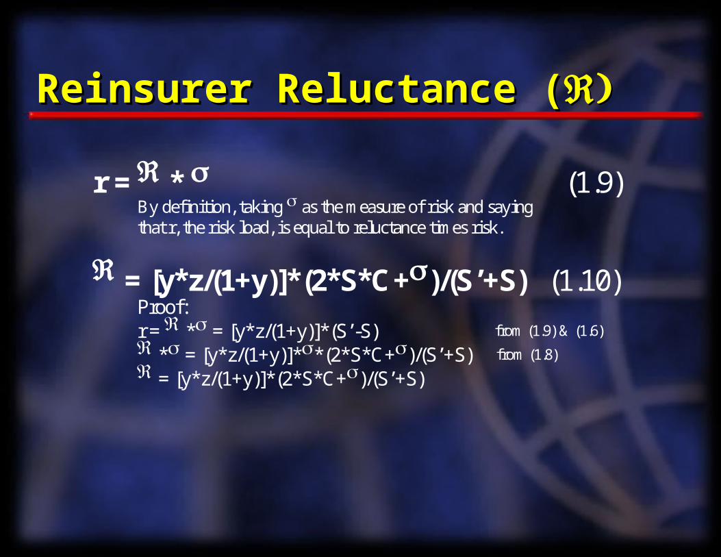
Reinsurer Reluctance (Reinsurer Reluctance (

r = * (1.9)By definition, taking as the measure of risk and sayingthat r, the risk load, is equal to reluctance times risk.

= [y*z/(1+y)]*(2*S*C+)/(S’+S) (1.10)Proof:r = * = [y*z/(1+y)]*(S’-S) from (1.9) & (1.6)

* = [y*z/(1+y)]**(2*S*C+)/(S’+S) from (1.8)

= [y*z/(1+y)]*(2*S*C+)/(S’+S)

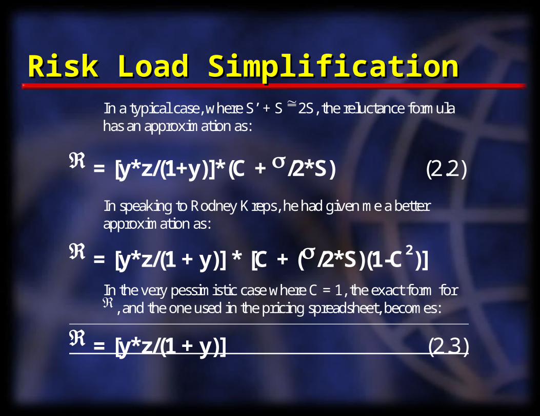
Risk Load SimplificationRisk Load SimplificationIn a typical case, where S’ + S 2S, the reluctance formulahas an approximation as:

= [y*z/(1+y)]*(C + /2*S) (2.2)

In speaking to Rodney Kreps, he had given me a betterapproximation as:

= [y*z/(1 + y)] * [C + (/2*S)(1-C2)]In the very pessimistic case where C = 1, the exact form for, and the one used in the pricing spreadsheet, becomes:

= [y*z/(1 + y)] (2.3)