Roofing Contractor Natick - J & R Construction (508) 620-9783
NASA Contractor Report 36 3 1
CARE III Phase III Report - Test and Evaluation
J. J. Stiffler, J. S. Neumann, and L. A. Bryant
CONTRACT NAS 1- 15 072 NOVEMBER 1982
https://ntrs.nasa.gov/search.jsp?R=19830004595 2020-01-24T12:03:00+00:00Z
TECH LIBRARY KAFB, NM
NASA Contractor Report 363 1
CARE III Phase III Report - Test and Evaluation
J. J. Stiffler, J. S. Neumann, and L. A. Bryant Raytheon Company Sudbury, Massachusetts
Prepared for Langley Research Center under Contract NAS l- 15 0 7 2
National Aeronautics and Space Administration
Scientific and Technical Information Branch
1982


TABLE OF CONTENTS GI_
1.0 INTRODUCTION . . . . . . . . . . . . . . . ..*...................................... 1
2.0 INTENT OF PHASE III . . . . . . . . . . . . . . . . . . . . . . . . . . . . . . . . . . . . . . . . . . . . . . . . . 2
2.1 Selection of Test Cases ......................................... 2
2.2 Description of Test Program Mathematical Model .................. 4
3.0 ACCOMPLISHMENTS . . . . . . . . . . . . . . . . . . . . . . . . . . . . . . . . . . . . . . . . . . . . . . . . . . . . . 8
3.1 Release One Evaluation .......................................... 8
3.1.1 Evaluation Procedure ....................................... 8
3.1.2 Evaluation Results .......................................... 8
3.1.3 Modifications Incorporated Into Second Release .............. 9
3.2 Release Two Evaluation .......................................... 10
3.2.1 Evaluation Procedure ........................................ 10
3.2.2 Evaluation Results .......................................... 10
3.2.3 Modifications Incorporated Into Third Release ............... 11
4.0 INTERPRETATION OF RESULTS . . . . . . . . . . . . . . . . . . . . . . . . . . . . . . . . . . . . . . . . . . . 13
4.1 Single-Fault Model Tests ........................................ 13
4.2 Double-Fault Model Tests ........................................ 15
4.3 Consistency Tests ............................................... 17
4.3.1 Test Cases Developed During This Phase ...................... 17
4.3.2 Test Cases Developed During PHASE I (FTMP) .................. 22
4.3.3 Test Cases Developed During PHASE I (SIFT) .................. 23
5.0 CONCLUSIONS AND RECOMMENDATIONS FOR FURTHER STUDY.................... 24
iii

TABLE OF CONTENTS (CONCLUDED)
PLOTTED FUNCTIONS ................................................... 26
RESULTS TABLES ...................................................... 120
Appendix 1 Program Listings
SFMODL ............................................................ 127
DFMODL ............................................................ 137
Appendix 2 Execution Field Lengths .................................. 145
Appendix 3 Select Test Cases ........................................ 146
Appendix 4 Coverage Functions ....................................... 149
References .......................................................... 156
iv

LIST OF FIGURES
FIGURE
I. CARE III SINGLE FAULT MODEL ........................... 6
II. CARE III DOUBLE FAULT MODEL ........................... 7
TEST CASE 1A
la FUNCTION PNB (LINEAR) CARE III MODEL .................. 26
la’ FUNCTION PNB (LINEAR) MARKOV MODEL .................... 27
lb FUNCTION PNB (LOG)CARE III MODEL ..................... 28
lb’ FUNCTION PNB (LOG) MARKOV MODEL ....................... 29
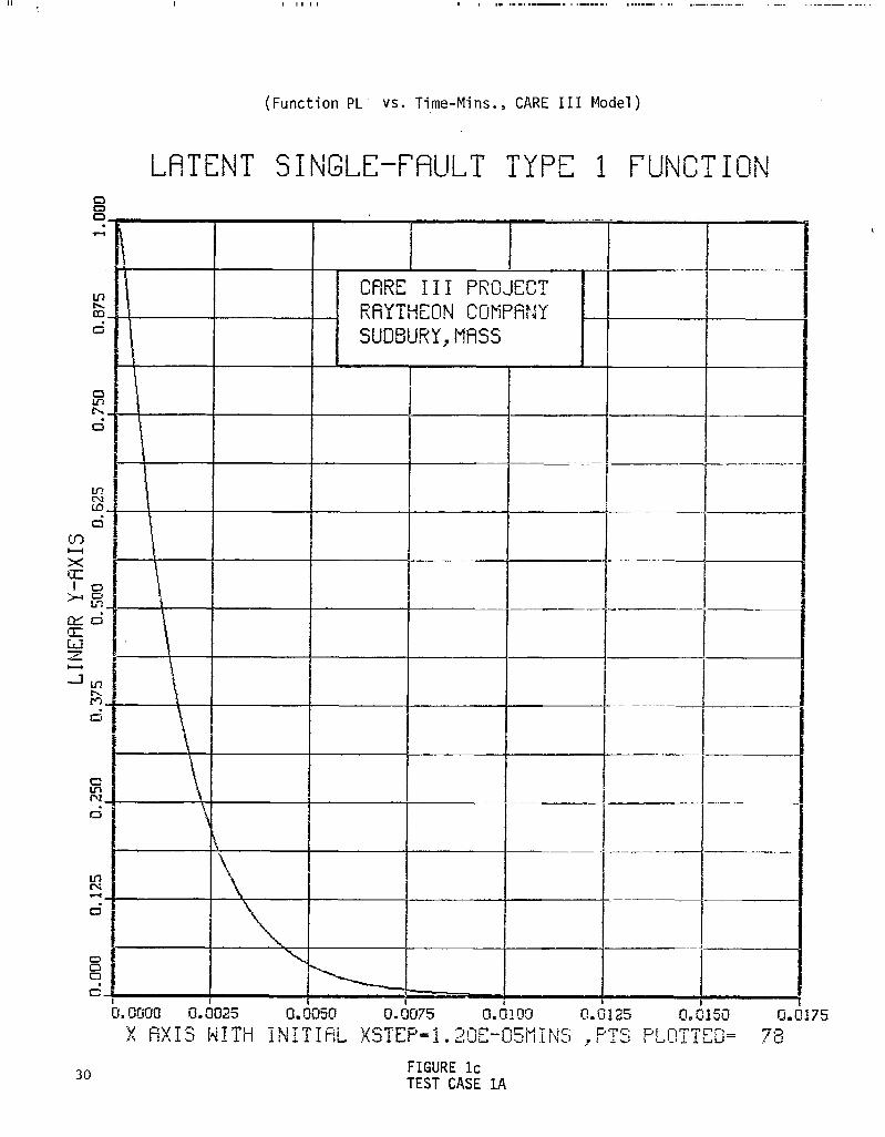
IC FUNCTION PL (LINEAR) CARE III MODEL ................... 30
lc’ FUNCTION PL (LINEAR) MARKOV MODEL ..................... 31
Id FUNCTION PL (LOG) CARE III MODEL ...................... 32
Id' FUNCTION PL (LOG) MARKOV MODEL ........................ 33
TEST CASE 2C
2a FUNCTION PDP (LOG-LOG) CARE III MODEL ................. 34
2a' FUNCTION PDP (LOG-LOG) MARKOV MODEL ................... 35
2b FUNCTION PB (LOG-LOG) CARE 111 MODEL .................. 36
2b' FUNCTION PB (LOG-LOG) MARKOV MODEL .................... 37
2c FUNCTION PNB (LOG-LOG) CARE III MODEL ................. 38
2c' FUNCTION PNB (LOG-LOG) MARKOV MODEL ................... 39
2d FUNCTION PL (LOG-LOG) CARE III MODEL .................. 40
2e FUNCTION Q SUM (LOG-LOG) CARE 111 MODEL ............... 41
2f FUNCTION P* SUM (LOG-LOG) CARE III MODEL .............. 42
&I FUNCTION Q+P* SUM (LOG-LOG) CARE III MODEL ............ 43

LIST 0F FIGURES (CONTINUED)
FIGURE
TEST CASE 3B'
3a FUNCTION PB (LINEAR) CARE III MODEL...................... 44
3a ’ FUNCTION PB (LOG) CARE III MODEL......................... 45
3a’ ’ FUNCTION PB (LOG-LOG) CARE III MODEL . . . . . . . . . . . . . . . . . . . . 46
3a "I FUNCTION PB (LOG-LOG) MARKOV MODEL....................... 47
3b FUNCTION PNB (LINEAR) CARE III MODEL..................... 48
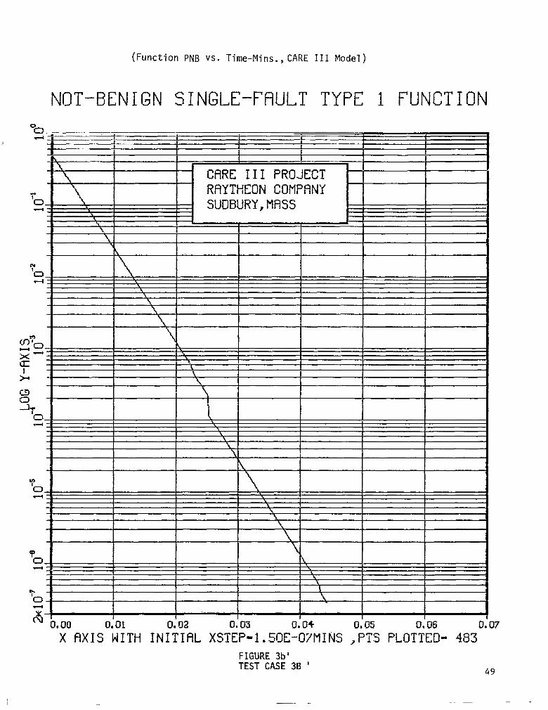
3b' FUNCTION PNB (LOG) CARE III MODEL........................ 49
3b" FUNCTION PNB (LOG-LOG) CARE III MODEL.................... 50
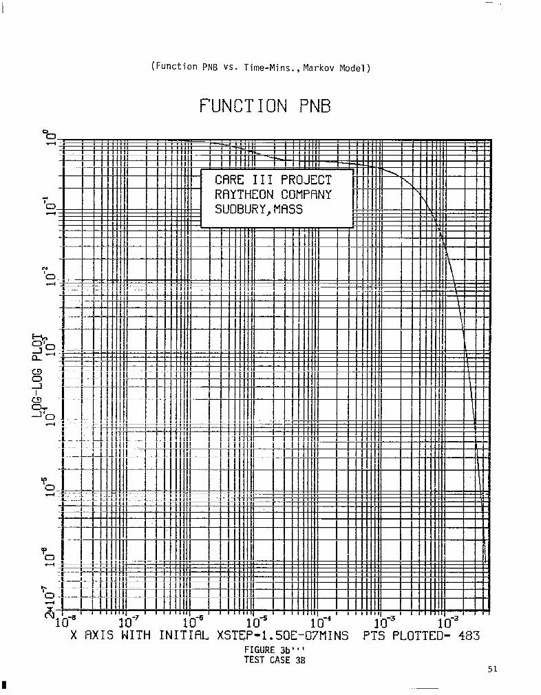
3b "I FUNCTION PNB (LOG-LOG) MARKOV MODEL...................... 51
3c FUNCTION PL (LINEAR) CARE III MODEL...................... 52
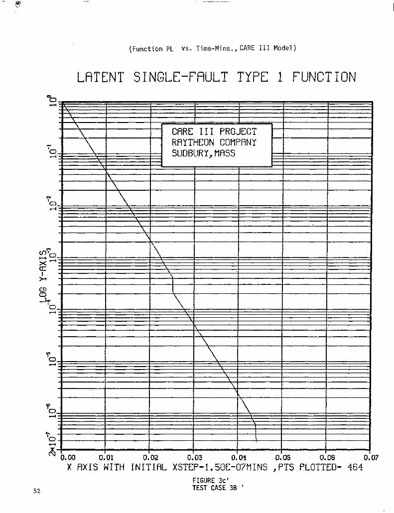
3c’ FUNCTION PL (LOG) CARE III MODEL......................... 53
3c’ ’ FUNCTION PL (LOG) CARE III MODEL......................... 54
3c “I FUNCTION PL (LOG-LOG) MARKOV MODEL....................... 55
3d FUNCTION PDF (1,l) (LINEAR) CARE III MODEL............... 56
3d' FUNCTION PDF (1,l) (LOG) CARE III MODEL.................. 57
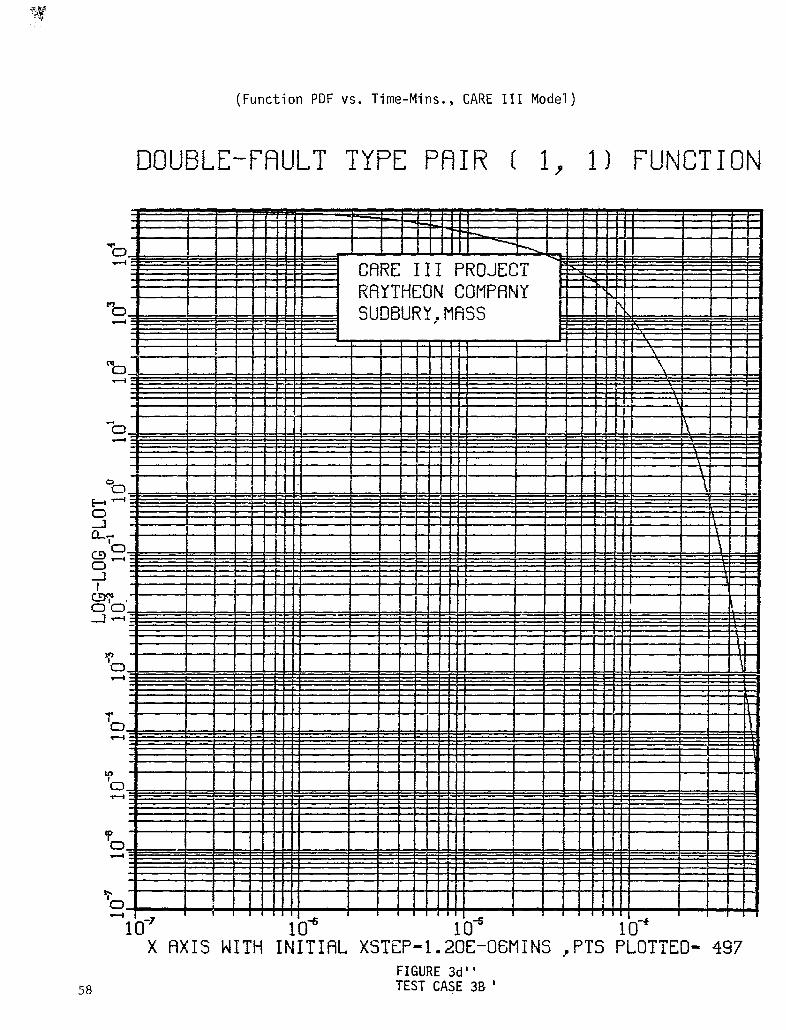
3d" FUNCTION PDF (1,l) (LOG-LOG) CARE III MODEL.............. 58
3e FUNCTION P* SUM (LOG-LOG) CARE 111 MODEL................. 59
3f FUNCTION Q SUM (LINEAR) CARE III MODEL................... 60
3f’ FUNCTION Q SUM (LOG) CARE III MODEL...................... 61
3f" FUNCTION Q SUM (LOG-LOG) CARE III MODEL.................. 62
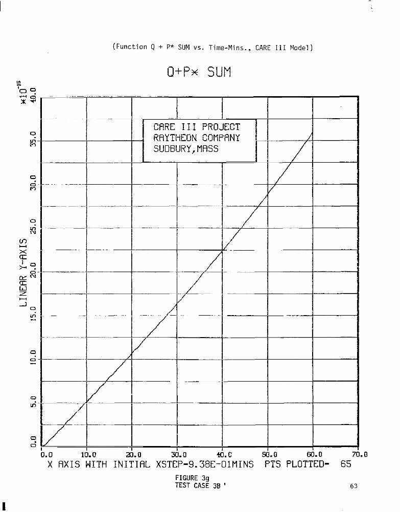
39 FUNCTION Q+P* SUM (LINEAR) CARE III MODEL................ 63
39' FUNCTION Q+P* SUM (LOG) CARE III MODEL................... 64
39' ' FUNCTION Q+P* SUM (LOG-LOG) CARE III MODEL............... 65

LIST 0F FIGURES (CONTINUED)
FIGURE
TEST CASE 3C/TRUNC = 10-4
4a
4a’
4b
4b'
4c
4c'
4d
4d'
4e
4e'
4f
4f'
49
4h
4i
4j
4k
41
4m
FUNCTION PB (LINEAR) CARE III MODEL ...................... 66
FUNCTION PB (LINEAR) MARKOV MODEL ........................ 67
FUNCTION PB (LOG) CARE III MODEL.........................6 8
FUNCTION PB (LOG) MARKOV MODEL ........................... 69
FUNCTION PNB (LINEAR)CARE III MODEL ..................... 70
FUNCTION PNB (LINEAR) MARKOV MODEL ....................... 71
FUNCTION PNB (LOG) CARE III MODEL ........................ 72
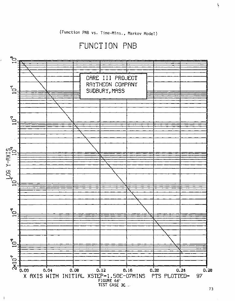
FUNCTION PNB (LOG) MARKOV MODEL .......................... 73
FUNCTION PL (LINEAR) CARE III MODEL ...................... 74
FUNCTION PL (LINEAR) MARKOV MODEL ........................ 75
FUNCTION PL (LOG) CARE III MODEL ......................... 76
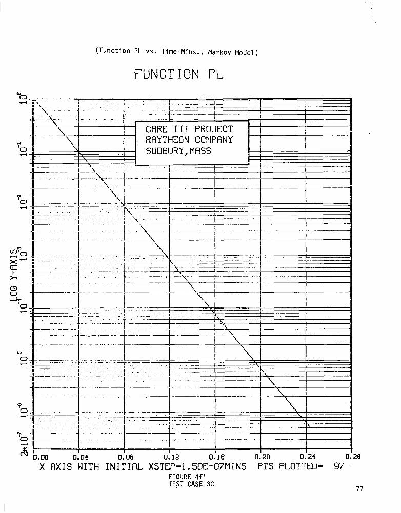
FUNCTION PL (LOG) MARKOV MODEL ........................... 77
FUNCTION PDF (1,l) (LINEAR) CARE III MODEL ............... 78
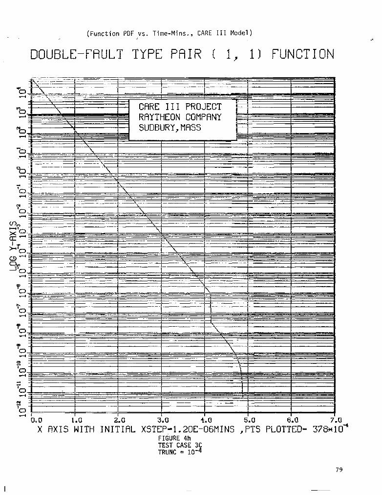
FUNCTION PDF (1,l) (LOG) CARE III MODEL .................. 79
FUNCTION Q SUM (LINEAR) CARE III MODEL ................... 80
FUNCTION Q SUM (LOG) CARE III MODEL ...................... 81
FUNCTION P* SUM (LOG-LOG) CARE III MODEL ................. 82
FUNCTION Q+P* SUM (LINEAR) CARE III MODEL ................ 83
FUNCTION Q+P* SUM (LOG) CARE III MODEL ................... 84
TEST CASE 3C/TRUNC = 10-6
4’a FUNCTION PB (LINEAR) CARE III MODEL...................... 85
4'b FUNCTION PB (LOG) CARE III MODEL......................... 86
vii

LIST OF FIGURES (CONTINUED)
FIGURE
TEST CASE 3C/TRUNC = 10-6 (CONT.)
4'c FUNCTION PNB (LINEAR) CARE III MODEL..................... 87
4'd FUNCTION PNB (LOG) CARE III MODEL ........................ 88
4'e FUNCTION PL (LINEAR) CARE III MODEL ...................... 89
4'f FUNCTION PL (LOG) CARE III MODEL ......................... 90
TEST CASE 3D'
5a FUNCTION PB (LINEAR) CARE III MODEL ...................... 91
5a' FUNCTION PB (LOG) CARE III MODEL ........................ 92
5a" FUNCTION PB (LOG-LOG) CARE 111 MODEL ..................... 93
5a "I FUNCTION PB (LOG-LOG) MARKOV MODEL ...................... 94
5b FUNCTION PNB (LOG-LOG) CARE 111 MODEL .................... 95
5b' FUNCTION PNB (LOG-LOG) MARKOV MODEL ...................... 96
5c FUNCTION PL (LINEAR) CARE 111 MODEL ...................... 97
5c' FUNCTION PL (LOG)CARE III MODEL .......................... 98
5c" FUNCTION PL (LOG-LOG) CARE III MODEL .................... 99
5c"' FUNCTION PL (LOG-LOG) FIARKOV MODEL ....................... 100
5d FUNCTION PDF (1,l) (LOG-LOG) CARE III MODEL .............. 101
5e FUNCTION Q SUM (LOG) CARE III MODEL ...................... 102
5f FUNCTION P* SUM (LOG-LOG) CARE III MODEL ................. 103
59 FUNCTION Q+P* SUM (LOG-LOG) CARE III MODEL ............... 104
TEST CASE 4A
6a FUNCTION PDF (1~) (LOG-LOG) CARE 111 MODEL.............. 105
6a' FUNCTION PDF (1,l) (LOG-LOG) MARKOV MODEL................ 106
viii

LIST OF FIGURES (CONCLUDED)
FIGURE
TEST CASE 4A (CONT.)
6b FUNCTION PDF (1,2) (LOG-LOG) CARE III MODEL............. 107
6b' FUNCTION PDF (1,2) (LOG-LOG) MARKOV MODEL ............... 108
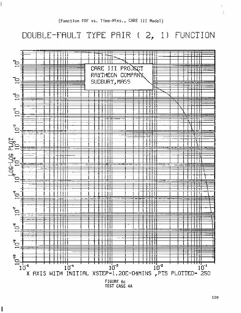
6c FUNCTION PDF (2,i) (LOG-LOG) CARE III MODEL ............. 109
6c' FUNCTION PDF (2,l) (LOG-LOG) MARKOV MODEL ............... 110
6d FUNCTION PDF (2,2) (LOG-LOG) CARE III MODEL ............. 111
6d' FUNCTION PDF (2,2) (LOG-LOG) MARKOV MODEL ............... 112
TEST CASE 4B
7a FUNCTION PDF (1,l) (LOG-LOG) CARE III MODEL ............. 113
7a' FUNCTION PDF (1,l) (LOG-LOG) MARKOV MODEL ............... 114
7b FUNCTION PDF (1,2) (LOG-LOG) CARE III MODEL ............. 115
7c FUNCTION PDF (2,l) (LOG-LOG) CARE III MODEL ............. 116
7c' FUNCTION PDF (2~) (LOG-LOG) MARKOV MODEL ............... 117
7d FUNCTION PDF (2,2) (LOG-LOG) CARE III MODEL ............. 118
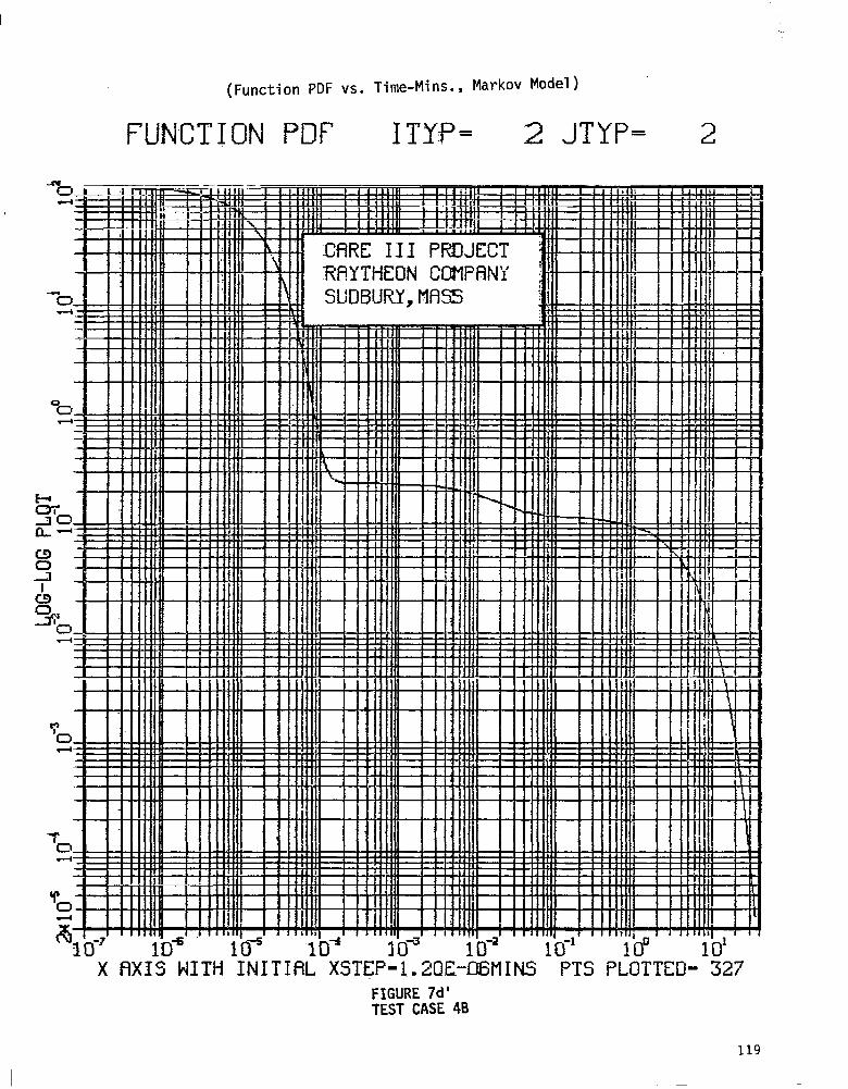
7d' FUNCTION PDF'(2,2) (LOG-LOG) MARKOV MODEL ............... 119
ix

LIST OF TABLES
TABLE
1. SINGLE FAULT TEST CASES AND RESULTS.................... 120
2. DOUBLE FAIJLT TEST CASES . . . . . . . . . . . . . . . . . . . . . . . . . . . . . . . . 123
3. F-IMP RESULTS . . . . . . . . . . . . . . . . . . . . . . . . . . . . . . . . . . . . . . . . . . . 124
4. SIFT RESULTS . . . . . . . . . . . . . . . . . . . . . . . . . . . . . . . . . . . . . . . . . . . 125

1.0 Introduction
The Phase III version of CARE III (Computer-Aided Reliability Estimation,
version three) is the product of a series of efforts designed to help estimate the
reliability of complex redundant systems. Although designed specifically
for use in fault-tolerant avionics systems, the approach is of a general nature
and can be used to model a variety of redundant structures.
The first CARE program developed at the Jet Propulsion Laboratory in 1971,
provided an aid for estimating the reliability of systems consisting of a com-
bination of any of several standard configurations (e.g.,stand by - replacement
configurations, triple modular redundant configurations, etc.). CARE II and CARE III
were subsequently developed by Raytheon, under contract to the NASA Langley Re-
search Center. CARE II substantially generalized the class of redundant config-
urations that could be accommodated, and included a coverage model to determine
the various coverage probabilities as a function of the applicable fault recovery
mechanism (detection delay, diagnostic scheduling interval, isolation and
recovery delay, etc.).
CARE III further generalized the class of system structures that can be modelled
and greatly expands the coverage model to take into account such effects as
intermittent and transient faults, latent faults, error propagation, etc. In
order to accomplish this, it was necessary to depart substantially from the
approaches taken in the earlier CARE efforts. The nature of, and reasons for,
this departure are discussed in the CARE III PHASE II Report, Mathematical Descrip-
tion, Section 2. This Phase III version of CARE III is a further refinement of
the CARE III approach, with the current status of the program reported on here.

2.0 INTENT OF PHASE III
The third phase of the CARE III project has been oriented towards the eval-
uation and refinement of the Phase II version of CARE III. Various stress tests,
single and double fault, and various consistancy tests have been defined so as to
test many of the assumptions and approximations used in the most recent version
of the program.
During the course of this evaluation a few inadequate numerical techniques
or their improper implementations have become apparent. Most of these inadequacies
have been corrected, although a few are beyond the scope of the current effort.
All of the problems encountered, their severity and the corrective actions taken
are addressed in this report.
2.1 Selection of Test Cases
Because CARE III is so versatile and the set of possible input conditions
so large, it is difficult to test it and to verify its accuracy with any degree
of completeness. The major emphasis of the current effort is to restrict the
allowed set of input parameters to the point that other, independent, but much
simpler models could be developed to verify at least some of the results produced
by CARE III. This approach was particularly useful in testing coverage model
results since these intermediate results had heretofore been tested only in-
directly through their influence on reliability predictions.
The specific test cases \rzre selected so as to minimize, in C.Al?E III, all factors
influencing unreliability except those that could be independently evaluated using
these simple models. These latter models were then used to verify the coverage functions
(e.g. PBct), Ps(t), PL(t), PDP(~), PDF(~)) (See Appendix 4 and Ref. 4) produced by CARE
III under various choices of the remaining unrestricted parameters. These parameters
were chosen specifically to stress the numerical analysis techniques
2

used in the CARE III coverage program, thereby attempting to expose any weak-
nesses in these techniques.
Other test cases, specifically, the FlMP and SIFT test cases, were
selected because previous results were available for comparison, both indepen-
dently derived results and results obtained using earlier versions of CARE III.
These tests were useful in assessing the effect on CARE III of the modifications
that have been introduced to improve its accuracy and to correct flaws discovered
during the aforementioned tests.
3
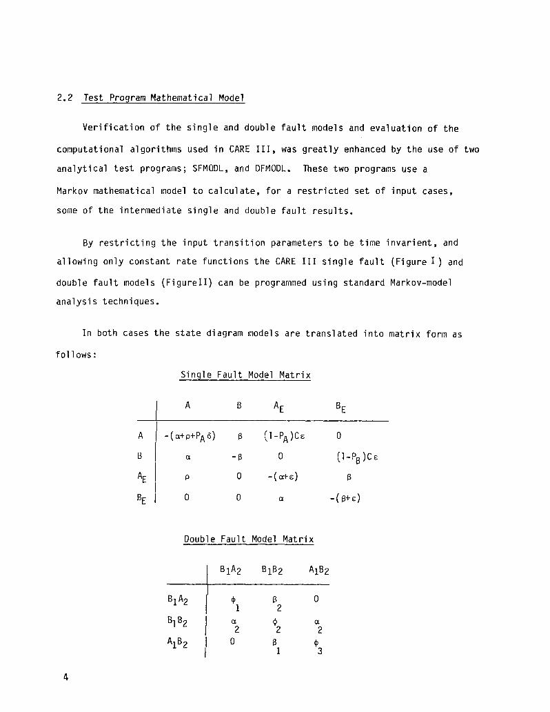
2.2 Test Program Mathematical Model
Verification of the single and double fault models and evaluation of the
computational algorithms used in CARE III, was greatly enhanced by the use of two
analytical test programs; SFMODL, and DFMODL. These two programs use a
Markov mathematical model to calculate, for a restricted set of input cases,
some of the intermediate single and double fault results.
By restricting the input transition parameters to be time invarient, and
allowing only constant rate functions the CARE III single fault (Figure I) and
double fault models (FigureII) can be programmed using standard Markov-model
analysis techniques.
In both cases the state diagram models are translated into matrix form as
follows:
Single Fault Model Matrix
A B AE BE
A I -(Ci+P+p& 6 (l-p/& 0
B a -B 0 $-pB)cE
0 -( a+E) B
0 a -( B+E)
Double Fault Model Matrix
] BlA2 BlB2 AlB2
BlA2 I
fb B 0 1 2
BlB2 I
a Q a 2 2 2
A$32 I 0 B + I 1 3
4
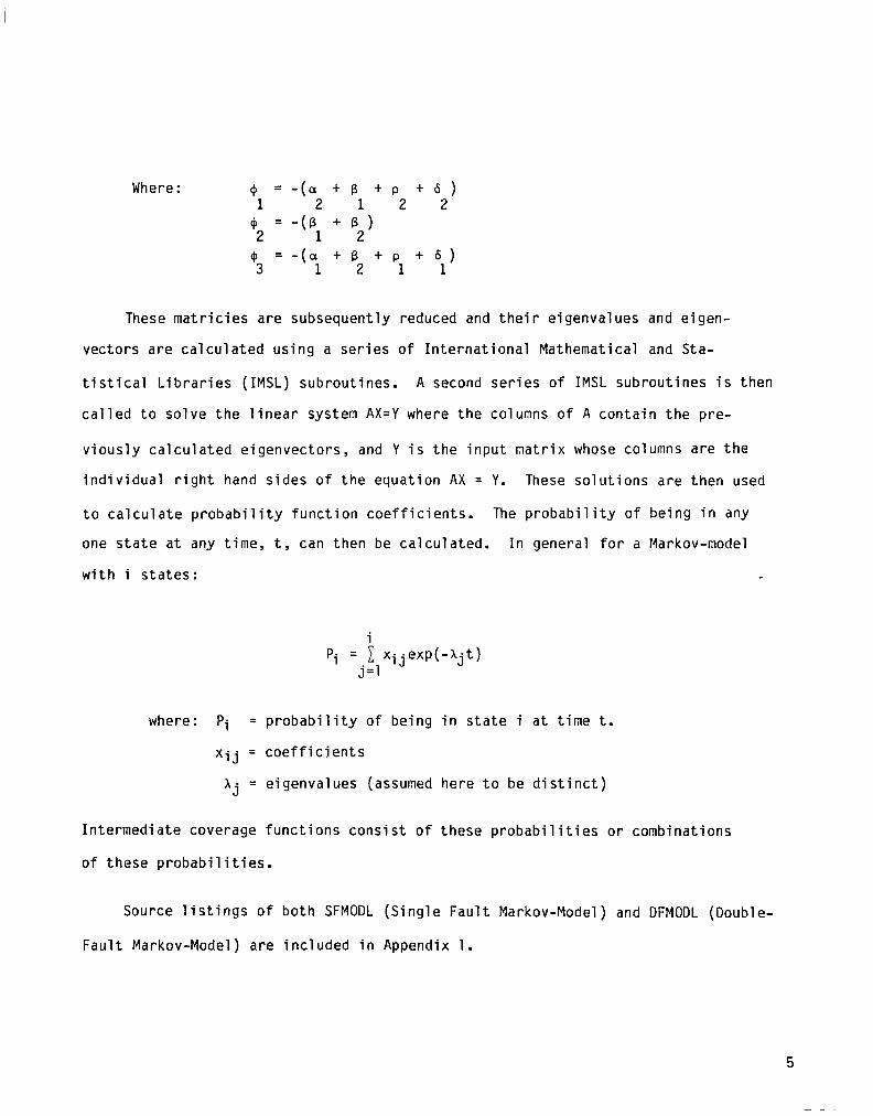
Where: $1 = -(a + B + P + 62) 2 12
@ = -(s + B2’ 2 + = 3
- ( a: + B2 + Pl + 9 1
These matricies are subsequently reduced and their eigenvalues and eigen-
vectors are calculated using a series of International Mathematical and Sta-
tistical Libraries (IMSL) subroutines. A second series of IMSL subroutines is then
called to solve the linear system AX=Y where the columns of A contain the pre-
viously calculated eigenvectors, and Y is the input matrix whose columns are the
individual right hand sides of the equation AX = Y. These solutions are then used
to calculate probability function coefficients. The probability of being in any
one state at any time, t, can then be calculated. In general for a Markov-model
with i states:
Pi = E XijeXp(-Ajt) j=l
where: Pi = probability of being in state i at time t.
xij = coefficients
9 = eigenvalues (assumed here to be distinct)
Intermediate coverage functions consist of these probabilities or combinations
of these probabilities.
Source listings of both SFMODL (Single Fault Markov-Model) and DFMODL (Double-
Fault Markov-Model) are included in Appendix 1.
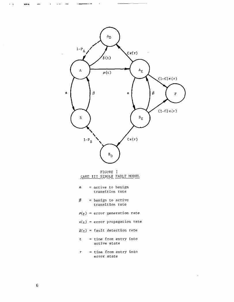
FIGURE 1 CARE III SINGLE FAULT MODEL --
a = active to benign transition rate
P = benign to active transition rate
P(t) = error generation rate
E(t) = error propagation rate
J(t) = fault detection rate
t = time from entry into active state
f = time from entry into error state

02 + q(t) + (l-P*
P, + P2W +
FIGURE 11
CARE III DOUBLE FAULT MODEL
7
I

3.0 Accomplishments
3.1 Release One Evaluation
3.1.1 Evaluation Procedure
The initial evaluation of CARE III began with a comparison of its results to
those obtained using the Markov-model program described above. The latter program
was used to determine, for one special case, the probability of a system failure
by time t (Q(t) values). This special case involved two stages, the first subject -2
to failures occurring at a rate X1 = 10 failures/hour, and the second failure
-20 occurring at a rate A2= 10 failures/hour. With no critical fault pairs,
and at time t << 20 hours the only significant contribution to a system failure
is a coverage failure in stage 1 (QlO (t)). A second, program was designed to
model transient faults in a similar fashion. The desired result in this case,
however, was not a failure probability, but instead the probability that a fault
has been detected as permanent by time t (PDP (t)). CARE III was run with iden-
tical inputs so as to derive results valid for comparison. The performance of
CARE II I under extreme conditions was also evaluated by running a series of stress
tests similar to those listed in Table 1. These stress cases include permanent,
transient, intermittent and software type fault tests.
3.1.2 Evaluation Results
The comparison between the test program results and the CARE III results, at
that time, were felt to be quite satisfactory, with some improvements to be gained
by modification of the coverage model integration routines (e.g. doubling criteria).

The transient fault comparison, however, highlighted two errors in numerical
computation:
1. The treatment of a function's steady state value. (For all times
t greater than the last calculated value, the function was equated
to zero).
2. An inconsistency with the function hDpT (tlXi) used in the defin-
ition of R,.(t) (ref. CARE III PHASE II Report, Mathematical Descrip- 1
tion, Table 1).
The results of the stress tests indicated some problems with accumulated
error generated while solving the VOLTERRA type integral.
3.1.3 ModificationsIncorporated Into Second Release
All of the above mentioned problems were addressed, and either corrected or
improved for the Phase III second release. A summary of the modifications made to
CAKE III during this period is as follows:
1. A self modifying capability was added to the doubling difference
parameter (DBLDF) (ref. CARE III PHASE II Report, User's Manual, Section
3.1) in COVRGE. In certain instances a DBLDF value may be appropr-
iate for all but a few of the functions. Under these conditions
DBLDF will be appropriatly modified, for that function only, and
that function will be recomputed. If the second attempt is unsuccess-
ful, a third try will not be attempted. Instead, the program will
be haulted with diagnostic messages printed. Additionally, array
sizes were increased to allow for smaller DBLDF values.
2. The inconsistency in the function Rx i
(t) was determined to be a
second, inappropriate, integration of HDPT (tlxi). This integration
was removed thereby correcting the calculation of Rx i
(t) in CARE3.
9

3. It was discovered that when the propagated error coverage proba-
bility C equals 1.0 and no critical fault pairs exist, zero valued
fault vectors were being unnecessarily computed. This was corrected in
the CARE3 program.
4. The unnecessary restriction of not allowing the X failure rate to be
greater than 1.0 in CAREIN was corrected. X may now be greater than 1.0.
5. The M input parameter was modified in CAREIN and CARE3 to allow
zero values, thereby providing a software fault modelling capability.
3.2 Release Two Evaluation
3.2.1 Evaluation Procedure
The procedure used to evaluate release 2 is essentially the same as that used
in the evaluation of release 1. The Markov-model programs were up-graded to include
several of the coverage single fault functions; PA, PB (benign), PNR (not benign),
PL (latent), and PDP (detected as permanent), in addition to the double fault func-
tion pg~. A greater emphasis was placed on the stress test results, both inter-
mediate and final, so as to characterize any sources of accumulated error allrl io
verify any assumptions used. A large part of the effort during this evaluation was
directed towards the more complicated and error prone coverage program (COVRGE).
3.2.2 Evaluation Results
Upon examination of the stress-test results it became apparent that accumu-
lated error in the integration routines is still a potential problem area.
Because of the extreme nature of these stress tests the integration
routines are forced to convolve functions whose maximum time, tmax, differ by
a much greater ratio than had been tested before. Any small amount of accumu-
lated error seen with standard cases becomes greatly magnified in these extreme
10

cases, to the extent that in one case (3d - see Table 1) an intermediate single
fault function (PA) became unbounded. A number of successful measures were
implemented to help rectify this situation.
3.2.3 Modifications Incorporated Into Third Release
The easiest and most obvious modification, although not without cost, was to
increase the array sizes, thereby allowing smaller initial step sizes. This modi-
fication improved the situation only slightly. It became apparent that it would be
desirable for the step-size doubling procedure to be changed to a halving pro-
cedure after a function has reached its peak (or valle
function decreases, as it peak is approached, the step
of doublings, and becomes quite large. This step size
ately capture the function as it again begins to rapid
). As the slope of the
size goes through a series
is then too large to accur-
y vary. Due to the nature
of COVRGE the incorporation of a halving ability was beyond the scope of this
phase. Instead, the doubling algorithm was modified to restrict doubling for 25
steps after a function peaks or dips. This approach has worked out as the most
effective compromise.
During this evaluation the single fault intermediate function Pa presented
the greatest problems. Because of the severe extremes of its constituent functions,
Pa was often the only unacceptable function. In order to make Pa less radical,
and hence more manageable, its numerical implementation was divided into a series
of smaller computations, with the more rapidly varying functions separated from the
slower varying functions. This approach was also successfully implemented in the
second single fault recursion, FX (t) (see Table 2A, CARE III PHASE II Report,
Mathematical Description).
The effect of these changes was two-fold; the acceptable range of input
parameters was greatly extended, and an increased accuracy was achieved for
the 'easier' input cases. In order to detect the few situations where
11

accumulated error could lead to erroneous results, a test has been incor-
porated into COVRGE to halt the program and produce a diagnostic message. Final
results will be erroneous if the following situation does not hold:
where I$I (t) = kernal of Fx X
A routine to test whether user inputs are within the value range, specified
in CARE III Phase II Report, User's Manual, was also incorporated into CAREIN
during this phase.
12

4. Interpretation of Results --
Some representative results of the tests conducted during this phase are
plotted in Figures l-7; other results are tabulated in Tables l-4. (See Appendix
3 for corresponding CARE III input files.) The figures emphasize comparison of the
coverage calculations obtained using CARE III to those obtained using the Markov-
model discussed in Section 2. Three types of plots are used to facilitate this
comparison: linear, log, and log-log.
The tables list the various parameters used in each test along with the
unreliability at user defined flight time (FT) determined by CARE III under each of
these sets of conditions. Since, in general, it is not possible to get an indepen-
dent verification of these results, their main value is as a reasonableness test -
do these results appear to be mutually consistant?
The tests can be conveniently grouped into three categories: single-fault-
model tests; double-fault-model tests, and consistency tests. Some observations
and conclusions about the tests in each of these categories are discussed in the
following paragraphs.
4.1 Single-Fault-Model Tests
The coverage and reliability parameters used in the single-fault-model tests
are listed in Table 1. Selected intermediate results obtained during these tests
are plotted in Figures 1 through 5 along with, wherever possible and appropriate,
the corresponding Markov-model results.
In general, the CARE III results and the Markov-model results compare
extremely well. The only discrepancies that appear to be significant are those
seen on the log plots. These discrepancies show up, however, only when the
function in question has become insignificantly small. In any case, they
13
I

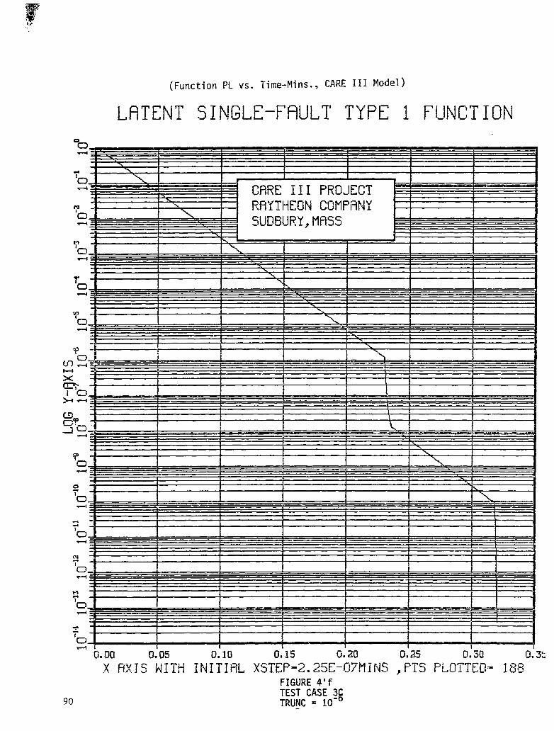
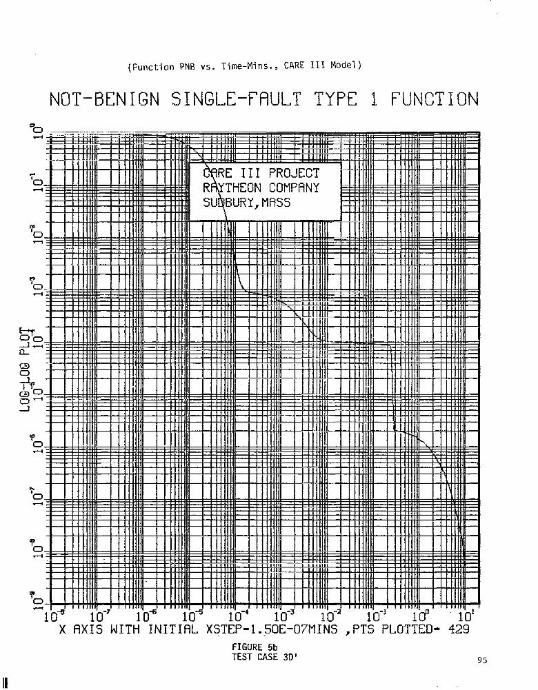
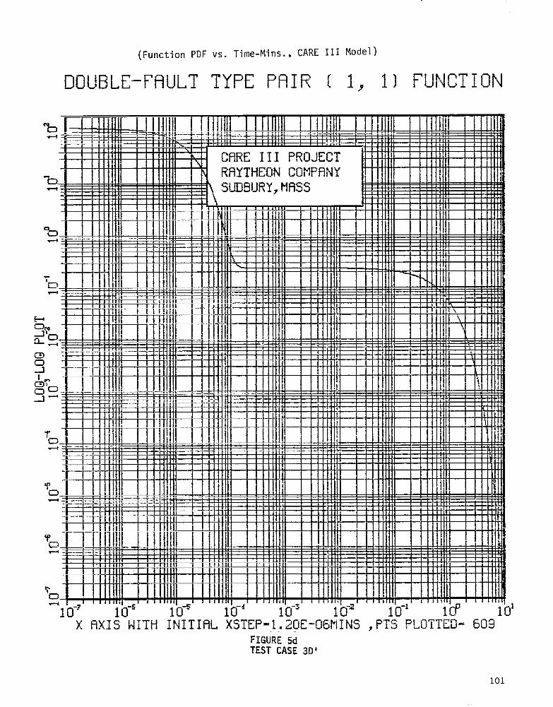
As previously noted, the test cases were deliberately selected to stress
some of the coverage model numerical evaluation procedures. One effect of this
is particularly evident in the log-log plots (and almost entirely obscured in the
linear and log plots) of Figure 3 and especially Figure 5. It is seen that several
of the coverage functions initially exhibit very rapid changes for a short interval
followed by a period of very slow changes followed, in turn, by another interval
of relatively rapid changes. Such functions severely stress the numerical integration
and recursion algorithms that require them as inputs. In order to accommodate the
initial, rapidly varying part of the function, the integration step size must be
ly small. In order to keep the time needed to eva luate the integration extreme
14
are caused by the fact that the CARE III model uses a user-specified parameter
(TRUNC) to determine when to truncate the calculation of an intermediate value
and set that value to zero. (The Markov-model does not need an analogous
parameter, since it, in effect, determines an analytic expression for the
function of interest). The discontinuities evident in the CARE III log plots
in Figures 1-5 are caused by these truncation events. This is easily seen by
comparing the plots in Figure 4 with the corresponding plots in Figure 4'.
TRUNC was changed from its normal l(t4 value in Figure 4 to a value of 10-6 in Figure
4’. As expected, the location of the discontinuities shifted and their
magnitude decreased with the decreased TRUNC value. It should be noted, how-
ever, that the effect of these discontinuities on the primary result of
interest (the system unreliability) is entirely negligible. The difference
between the TRUNC = 10-4 and TRUNC = 1(~6 unreliabilities predicted by CARE III
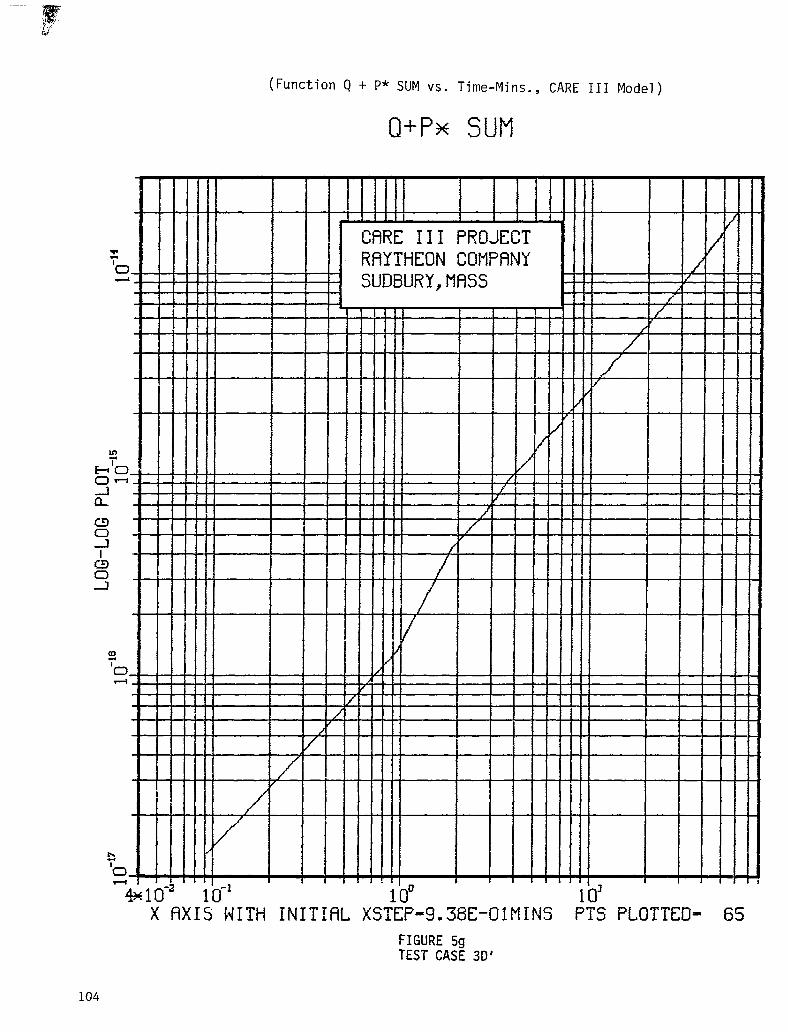
for the Figure 4/4' test case, in particular, is .002%. The same truncation effect,
incidently, explains the discontinuities seen in the P* and Q plots in Figures
l-7; again, these discontinuities are insignificant so far as the results of inter-
est are concerned.

from becoming excessive, the step size must be allowed to increase rapidly as the
rate of change of the function decreases. Unfortunately, any step size selection
rule compatible with both of these requirements tends to introduce significant
error when the function again begins its rapid variation. It was to accommodate
such functions that some of the modifications discussed in Section 3.2.2 were intro-
duced. Their effectiveness can be seen by comparing the log-log plots of the CARE
III results and those obtained using the Markov-model.
One area in which CARE III evidently still needs work is the transient model.
As seen in Figure 2, the P* results (and hence the Pf t Q results) tend to oscillate.
Apparently, this is due to round-off error resulting from the calculation of Rx(t),
the reliability of an element subject to well-covered transients (so that R,(t )-1)
and then using 1 -R,(t) in subsequent calculations. Such oscillations are clearly
incorrect and the evaluation procedures should be modified to remove them. This
should not be difficult to do; unfortunately, time and budget constraints prevented
this from being accomplished as part of the current effort.
4.2 Double-Fault-Model Tests
A Markov-model was also written to provide a means of evaluating independently
some of the CARE III coverage functions associated with the double-fault model.
The postulated double-fault model test cases are listed in Tible 2. Again because
of time and budget constraints, only two of these test cases were actually run.
The results of these runs are shown in Figures 6 and 7.
In general, the agreement between the Markov-model and the CARE III results
appear to be satisfactory, although less exact than the agreement between the
single-fault model results. This is somewhat surprising since the CARE III double-

-fault model uses techniques similar to those used in the single-fault model, and
the model itself is considerably simpler. It is believed that modifications to
the CARE III double-fault model numerical evaluation procedures similar to those
made in the single-fault case would virtually eliminate these discrepancies.
Again, however, time and budget constraints precluded this effort.
It should be remarked that the differences in the two sets of results could be
at least in part due to inaccuracies in the Markov-model results. The Markov-
model, for example, was unable to produce any answer in the double (1,2) fault
case for test 4B, (cf. Table 2). This particular case is especially interesting
in that CARE III produces a bimodal curve for the intensity of double-fault
coverage failures, PDF(t) (Figure 7b). Since the Markov-model did not work in this
case, and since bimodal coverage function curves are apparently unusual, the ques-
tion arises as to whether this result is actually valid. An examination of the
physical situation being modelled, however, suggests that the results are at least
approximately correct. *
The only difference between the first-occurring and second-occurring faults
in this case is that the former has an active-to-benign transition rate of
l/set. while the latter has an active-to-benign transition rate of lOOO/sec.
Since the first fault must be benign when the second fault occurs (otherwise L.
the system would fail immediately), and since the benign-to-active transition
rate for both faults is slow (l/set.) relative to the active-to-benign transition
rate of the second fault, the rate of change of pDF is dominated entirely by
the active-to-benign transitions of the second fault. It is easily verified,
in fact, that the initial value of 4F(t) is B+p = 120/min. This initial
activity should persist for only about .OOl seconds (1.6 x lG-smin.), since
that is the expected time for the second fault to become benign. Since no double-
*An alternate Markov modeling technique at NASA-Langley did reproduce the CARE III results.
16

fault failure can occur when both faults are benign, the value of PDF(t) should
decrease significantly at this point. Since the benign-to-active transition
of both faults are identical (l/set.), exactly half of the transitions out of
the doubly benign state will be to the state in which the first fault is active
and the second is benign. The occupancy probability of this state should peak
at roughly 1 second (.016 mins.). Furthermore, since transitions from this
state back to the doubly benign state occur at the relatively slow l/set.
rate, the rate of change of mF(t) following this second peak should be much
slower than that following the first peak. These observations describe precise-
ly the results predicted by CARE III (remember that the Figure 7 plots are log-log
plots), thus verifying, at least qualitatively, that the CARE III double-fault
coverage model is performing correctly in this otherwise unverified case.
4.3 Consistency Tests
Consistency tests run during this phase were of two types: 1) The test cases
developed during this phase and used primarily to test the single-and double-
fault coverage models were also allowed to run to completion, thereby producing
reliability estimations that could be compared from test to test and evaluated
for consistency. 2) Some of the test cases run during Phase I of the CARE III
program were re-run, again to verify consistency of results and to determine
whether any of the changes made during this phase of the program significantly
altered any of the earlier results.
4.3.1 Test Cases Developed During This Phase
Several observations can be made concerning the consistency of the results
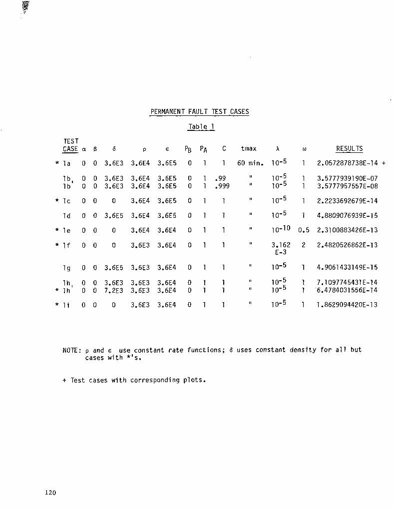
presented in Table 1:
1) The failure probablity decreases when the error propagation
rate increases if C = 1 and all other parameters remain the same
17

(compare test cases la and lh, lc and li, Id and lg). This initially
counter-intuitive result is clearly correct when it is observed
that, when C = 1, al 1 propagated errors are detected; thus,
the quicker they propagate, the shorter the latency of the fault.
2) The previous statement also holds for long-term transients
(compare test cases 2c and 2~') but the reverse holds for short-term
transients (test cases 2a and 2a'). This can be explained by the fact
that, while transients behave much like permanent faults if the
active period of the fault is long compared to the other coverage
parameters, the quick propagation of errors resulting from short-
term transients increases the likelihood that they are detected as
permanent (PA=1 , 4 =o) . Since the latency period for short-term
transients is, by definition, short in any event, this latter
effect dominates.
3) When the probability that any unit survives for the interval of
interest is kept constant, the effect of a nonconstant hazard rate
is to increase the failure probability regardless of whether the
hazard rate is an increasing or a decreasing function of time
(compare the numerical results of test case lh with cases le and lf).
This is clearly true, since a non-uniform hazard rate concentrates the
failures at the beginning (when the hazard rate is decreasing function of
time) or at the end (when it increases with time) of the interval in
question. In either case, the likelihood of double faults is increased.
4) A less-than-perfect probability of detecting propagated errors can
have a profound effect on the probability of system failure
18

(compare test cases lb and lb' with all the others). These results
can even be roughly verified quantitatively. When C=l, coverage
failures occur only when one fault occurs within the latency period
of an earlier fault. Since the latency of a fault is of the order
of the faster of the fault detection and error propagation delays
(reciprocal rates), it is typically of the order of 0.1 to 1 second,
or about 0.01% of the total interval of concern here. Thus, the probability
of failure due to a double fault is roughly 10s4$ with q the probability
0f.a single fault. The probablity of a failure due to an uncovered
single fault is roughly (1-C)q. Since q is approximately 10e5 here,
this argument would predict a double-fault failure probability of
roughly lo-l4 and a single-fault failure probablity of 10s7 when
C=.99 and 10-S when C=.999, thus supporting the observed results.
5) A constant fault-detection rate is somewhat less effective
than a constant fault-detection density function (compare test cases
lh and lh'). When faults are detected at a constant rate G/set.,
the probability that a fault has not been detected after being
active for t seconds is e-6t. When the fault detection density
function is a constant G/set., this same probability takes the
form 1-62 (O<t<l/s). Since e-fit>(l-8t) for all O<&tcl, this
result is obviously correct.
A constant-rate fault-detection function results, for
exanple, when a diagnostic program is randomly scheduled; a
constant-density function results when it is run on a,fixed
schedule. Equating the two h-parameters is meaningful, since doing
19
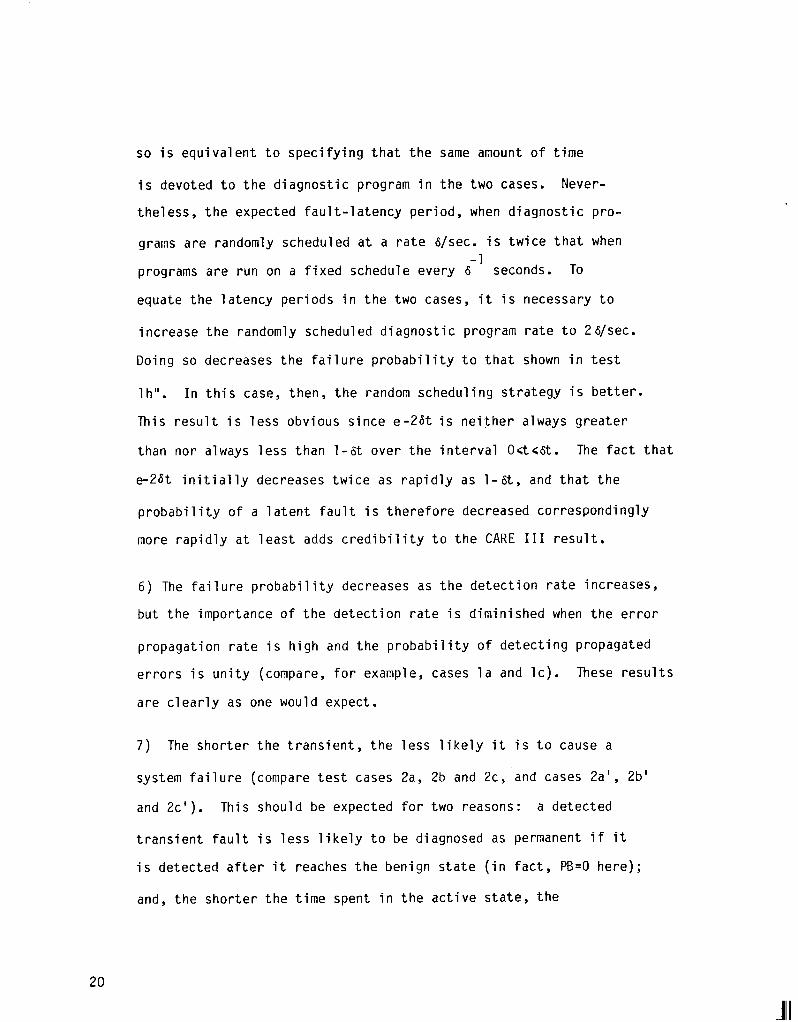
so is equivalent to specifying that the same amount of time
is devoted to the diagnostic program in the two cases. Never-
theless, the expected fault-latency period, when diagnostic pro-
grams are randomly scheduled at a rate G/set. is twice that when -1
programs are run on a fixed schedule every 6 seconds. To
equate the latency periods in the two cases, it is necessary to
increase the randomly scheduled diagnostic program rate to 2&/sec.
Doing so decreases the failure probability to that shown in test
lh". In this case, then, the random scheduling strategy is better.
This result is less obvious since e-26t is neither always greater
than nor always less than l-At over the interval O&c&t. The fact that
e-26t initially decreases twice as rapidly as l-&t, and that the
probability of a latent fault is therefore decreased correspondingly
more rapidly at least adds credibility to the CARE I II result.
6) The failure probability decreases as the detection rate increases,
but the importance of the detection rate is diminished when the error
propagation rate is high and the probability of detecting propagated
errors is unity (compare, for example, cases la and lc). These results
are clearly as one would expect.
7) The shorter the transient, the less likely it is to cause a
system failure (compare test cases 2a, 2b and 2c, and cases 2a', 2b'
and 2~'). This should be expected for two reasons: a detected
transient fault is less likely to be diagnosed as permanent if it
is detected after it reaches the benign state (in fact, PB=O here);
and, the shorter the time spent in the active state, the
20

less likely will the effect of the fault be present at the time
of a subsequent fault.
8) The effect of an intermittant fault depends both on the frac-
tion of time it spends in the active state (contrast test cases 3a and 3b
with test case 3d, for example) and on the rates at which it makes transi-
tions between these states. At least when propagated errors are
certain to be detected, it is significantly worse for a fault to be
almost always benign than for it to be almost always active (compare,
for example, test cases 3c" and 3d"). The result is due to the fact that
the more time a fault spends in the active state, the more quickly
it will be detected and hence the less likely it will contribute to
a system failure (since C=l). This is apparently (but not obviously)
more significant than the fact that a fault is harmless when it is
in the benign state. That this last statement is true is suggested
by the following agruoent. Suppose that two intermittant faults
simultaneously exist for PI units of time and that each is active
during a given unit of time with probability l/N, independent both of
the other fault and of its own past. Then the probability that the
two are never simultaneously active is (l-l/N) 2N
which, for large N,
is roughly em2 = .14. If the two simultaneously exist for only half
as long (N/2 time units) this probability increases, but it is still -1
only e = .37. Thus, even though both faults are almost always benign,
the fact that they exist for an extended interval make the probability
quite large that they are, at some instant, both active (and hence
cause the system to fail). Thus, again, the observed results appear
to be at least qualitatively consistent.
23

9) Additional consistency checks can be made by comparing the
results for different types of faults when the parameters are
such that their differences should be relatively insignifi-
cant. As already observed, for example, when intermittants
spend most of the time in the active state they tend to look
like permanent faults. This is confirmed by comparing the
results of case 3c with those of case li.
4.3.2 Test Cases Developed During Phase I (FTMP)
Consistency during the evaluation of CARE III can be seen by examining the
results of Table 3. This table tabulates the results of the Fault Tolerant Multi-
Processor (FTMP) test cases for a number of CARE III versions. Included are some
of the results reported on in the CARE III Final Report, Phase I, Volume I
(Table 3.3), the Phase II (release 1) results, and the current Phase III (release
3) results.
As can be seen, there is a consistent trend in the results predicted by
CARE III for each of the versions tabulated, the severity of which is pro-
portional to the ratio a/B. This is evidently a consequence of the different
restrictions placed on these models. In order to reduce the complexity of the
Draper model, any three simultaneous latent faults were equated to a system fail-
ure. The Phase .I model identifies three simultaneous latent faults with a system
failure only if at least two of these faults constitute a critical pair. The
Phase II model eliminates all restrictions on the number of simultaneous latent
faults; a system failure occurs only when both faults in a critical pair are
simultaneously active. This aspect of the model was not changed in Phase III. The
differences between the release 1 and release 3 results can be accounted for by
22

the changes made to the way in which coverage results are used in the re
bility evaluations. In general, these changes resulted in tighter upper
bounds on unreliability by eliminating double counting (e.g. by eliminat
ia-
w
the possibility that the same fault leads to two system failures by being
involved, possibly at different times, in two critical pairs). As would be
become more apparent
fault remains latent is
expected, the effects of these different restrictions
as the ratio a/B increases since the amount of time a
an increasing function of this ratio.
4.3.3 ;
Similar comparisons were made between the reliab
Software Implemented Fault Tolerance (SIFT) computer,
and those produced by the Phase I version of CARE III
the current CARE III (Table 4).
ility predictions for the
both those derived by SR
3 with those generated by
I
In Phase I the coverage model had not yet been programmed, so the coverage
inputs to the reliability program were those corresponding to the SRI model in
which every fault has a latency of exactly T seconds. The CARE III coverage
model does not allow constant-time latency periods (although this capability
could be included if it were of general interest). Consequently, CARE III was
exercised, for these examples, using a constant-density fault detection function
with a T seconds mean-time to detection. This is obviously only a rough
approximation to a constant T second detection delay. Even so, the results
thus obtained compare very well with those derived both by CARE III using
the simulated coverage model inputs and by SRI, thereby giving added credence
to the current version of CARE III.
23

5.0 Conclusions and Recommendations for Further Study
In general, the CARE III results are in excellent agreement with those
derived independently, at least in those restricted cases in which independent
evaluation is readily obtained. There remain some flaws in CARE III, however,
which could not be eliminated under the current budget and schedule constraints.
Specifically, the transient model produces results that show instabilities
at least under certain conditions, and the double-fault model is less accurate
than it should be.
The following recommendations for further study are suggested by the re-
sults obtained during this effort:
1. Obviously, the flaws uncovered in the transient and double-fault
cases should be analyzed and eliminated.
2. Since it is believed that many of the problems encountered during
those tests, including those in the double-fault model, have to do
with the fact that the integration routine step size can be changed
adaptively only by doubling it, this restriction should be removed.
This restriction was initially felt to be acceptable since it was
believed that coverage functions tended to have monotonically
decreasing derivatives. This is evidently not the case.
3. Under certain conditions, the coverage model evaluation was found
to take an excessive amount of computer time. This problem could
be eliminated by the integration routine modification recommended
above. In addition, however, it is recommended that an alter-
native, Markov-type coverage model, similar to that described
in Section 2.2, be incorporated into CARE III to be used whenever
the user specifies only constant rate coverage parameters.
Although this case is, somewhat restrictive, it is expected to
be the one most commonly used. Even when it is not precisely
24

applicable, it could be used to obtain preliminary results and to
screen out those conditions meriting more careful and more pre-
cise scrutiny. When the Markov-model can be used, the run time
in many cases could be drastically reduced.
4. Although the testing accomplished here has significantly in-
creased our confidence in CARE III, it can by no means be
asserted that CARE III has been completely verified. Further
testing is highly recommended.
25

(Function PNB vs. Time-Mins., CARE III Model)
NOT-BENIGN SINGLE-FRULT TYPE 1 lCUNCTION
CARE III PROJECT RAYTHEGN COHPaNY SUDBUKY, MRSS
26

(Function PNB vs. Time-Mins., Markov Model)
FUNCTION PNB
I
CARE III PROJECT RAYTHEON COMPflNY SU!lBlJRY, MASS
\ I I I !
0.000 0.002 X HXIS WITH
O.OM
INITIAL 0.006 0.008 0.010
XSTEP-1.20E-OSMINS PTS FIGURE la’
0.012 PLOTTED-
I
TEST CASE 1A 27

: --‘-- -- _...
(Function PNB VS. Time-Mins., CARE III Model)
NOT-BENIGN SINGLE-FAULT TYPE 1 FUNCTION
RAYTHEON COMFANY
-r 0 4
I , I ..I I I 1 I
i - - I I I
‘: 0
- 0.0000 I I I
O.C~O25 Q.Ocm G. GO75 Cl.@!00 cLG12S C.OlX 0. !75
28 FIGURE lb TEST CASE lpi

(Function PNB vs. Time-Mins., Markov Model)
FUNCTION PNB “0 “0
I I 4 4
CflRE III PROJECT CflRE III PROJECT RRYTHEON COMPANY RRYTHEON COMPANY
m ix000 0.000 0.002 o.'cloz ohot O.OW Oh06 0.006 Oh06 0.006 0.010 O.blO cl.012 0, 0, X AXIS WITH INITIAL XSTEP-1.20E-OSMINS PTS PLOTTED- 73
FIGURE lb TEST CASE 1A
” .
(Function PL vs. Time-Mins., CARE III Model)
LATENT SINGLE-FAULT TYPE 1 FUNCTION
RAYTHEON CORPFi!:Y SUmJRY, MASS
I
0. GOOU 0.0025
30 FIGURE lc TEST CASE 1A

(Function PL VS. Time-Mins., Markov Model)
FUNCTION f'L
CARE III PROJECT RAYTHEON COMPENY SUDBURY,MASS
. 000 0.002 0. oat 0.006 0.006 0.010 0.012 X AXIS I4ITH INITIftL XSTEP-1.20E-OSMINS PTS PLOTTED-
FIGURE lc’ TEST CASE 1A

c
(Function PL vs. Time-Mins., CARE III Hodel)
LATENT SINGLE-FAULT TYPE 1 FUNCTION
CFiRE III PROJECT RAYTHEON COM!=i=!NY
32
. . 0.9ml o.bo25
FIGURE Id TEST CASE lA_-

(Function PL vs. Time-Mins., Markov Model)
FUNCTION FL
CARE III PROJECT RAYTHEON COMPRNY
000 0.002 0.003 0.006 0.008 0.010 O.fJl2 X AXIS WITH INITIAL XSTEP-1.20E-OSMINS PTS PLOTTED= 73’
11t
FIGURE Id’ TEST CASE 1A 33

(Function PDP vs. Time-Mins., CARE III Model)
PERMANENT SINGLE-FAULT TYPE 1 FUNCTION
FIGURE 2a TEST CASE 2C

(Function PDP vs. Time-Mins., Markov Model)
FUNCTION PDP
FIGURE 2a' TEST CASE 2C 35

-(Function PB vs. Time-Mins., CARE III Model)
BENIGN SINGLE-FAULT TYPE 1 FUNCTION
.
36
X AXIS WITH INITIAL XSTEP-l.SOE-06MINS ,PTS PLOTTED- 83 FIGURE 2b TEST CASE .2C

(Function PB vs. Time-Mins., Markov Model)
FUNCTION PB
FIGURE 2b' TEST CASE ?C 37

(Function PNB vs. Time-Mins., CARE
NOT-BENIGN SINGLE-FAULT 4
III Model)
TYPE 1 FUNCTION
RAYTHEl-N COMPANY
I 1 I I,,,,,,,
T i I 1 I11~111 I Illl’ll I I. I .l.l.L~ILLI..-.-t
-. I I llllil!~ I
II Illill - him I I 1111111 I
I I I I I111111
I
I I Illlill
I I 1111111 I I I111111 I I I I ill1 IIIi
. . 1 Ill1,11l ~ . . . I 1 Iilllii -1 I i .I i.liil- -..I --LE
I I I111111 I I1111111 I I I I iI’/ I.
I I I111111 I i Illlill I I I I Ilill I l111111
X AXIS WITH INITIAL XSTEP-1.20E-OSMINS ,PTS PLOTTED- FIGURE 2c
38 TEST CASE 2C

(Function PNB vs. Time-Mins., Markov Model)
FUNCTION PNB
CRRE III PROJECT RAYTHEON COMPANY
. , . . . . c l-
llll1.I
I I I l-tll 5 I I r. I I I I Ill11 I I I I If-ill I I I 1 I1111 I I 1111111 \ I I
I I *:,,,,, I I ll,,l1l I I I I Ill1111 I I1111111 I I I Ill11 I I I111111 L! I
1 I 111111 I I1111111 I I 11111;1 I I llllli I I III I I
I I I1111111 I 11111111 I I I I I I I11111 I I
.05 lb4 I 111,111,
1 o-3 I I Illll1~
1O-2 X AXIS WITH INITIAL XSTEP-1.2aE-OSMINS PTS PLOTTED- 91
FTCIIRF 3r’
i &““I.b L-b
'EST CASE 2C 39

(Function PL vs. Time-Mins., CARE III Model)
40
LATENT SINGLE-FflULT TYPE 1 FUNCTION
I I : a,,,, 1
‘;_ 1 I I I Iliii i---hi I I lllii I I
I I Illltl I I 11111111 1 I I III CARE III PROJECT RAYTHEON COMPANY
r! I I i1lill I Iiliili I I1111111 1 (1 ‘I,,{ I i
‘cl I III I I I I II111
-10” I I Ill11
lb I I IllllI I I111111~ I
10” 1o-3 lo-2 X AXIS b!ITH INITIAL XSTEP-l.ZOE-OSMINS ,PTS PLOTTED- 90
FIGURE 2d TEST CASE 2C

(Function Q SUM vs. Time-Mins., CARE II.1 Model)
Cl SUM
CARE III PROJECT RAYTHEON COMPFiNY
I I IIll I I I I I I II I
I I I i iirii
I I I I 1 I I I IlkIll I I I I It I
‘0 a I I I II 111 I
$&2 ’ 10-I I I II III I I I ,,I,,, I 81 III I I,,1111 I I III
lo” 10’ ’ X AXIS WITH INITIAL XSTEP-9.38E-OlMINS PTS PLOTTED- 65
FIGURE 2e TEST CASE 2C 41
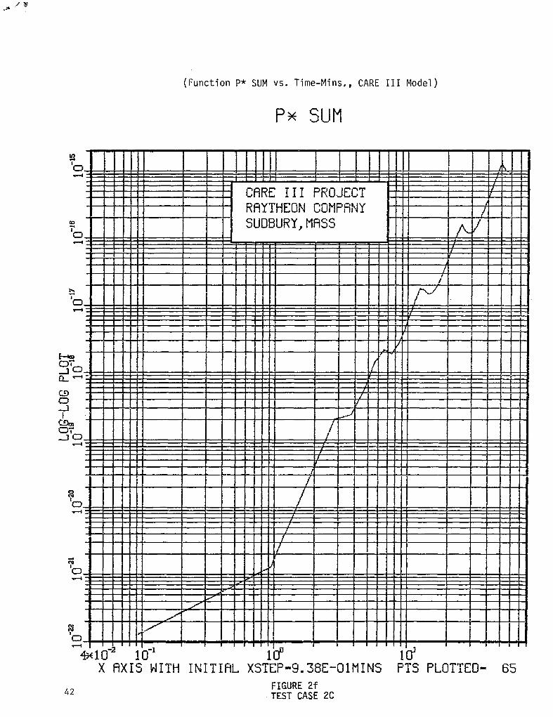
(Function P* SUM vs. Time-Mins,, CARE III Model)
Px SUM
CRRE III PROJECT RflYTHEON COMPFiNY
I I ,111, I I I ,,,I!, I I I1,1!1, 1 I I I I1111 I I I !lll!l I I i 111111 /I I I ill
III I Ill1 I i
. I I IIll I I I I I I I I,,
II 1
P 1
I 0 I
-is 1 O-2 1 , 8 I I 1 I I I I I 10-l lo” lo’
42
X AXIS WITH INITIAL XSTEP-9.38E-OlMINS PTS PLOTTED- 65 FIGURE 2f TEST CASE 2C

(Function Q + P* SUM vs. Time-Mins., CARE III Model)
Q+f’x SUM --.. _ ._ .-
In ’ “1
1 !! !!!!
I I I111111 I I I IllI 7
0 4 -
I I
IA ..--.I. ~oii~-..~!
.
-& &2
- ! 1 I
I l o-l
lo” LO’ ’
X AXIS WITH INITIAL XSTEP-9.38E-OlMINS PTS PLOTTED- 65 FIGURE 2g TEST CASE 2C 43

(Function PB vs. Time-Mins., CARE III Model)
BENIGN SINGLE-FAULT TYPE 1 FUNCTION aD
44
RAYTHEON COMPANY
too on-o1 0;oz 0:03 o;o+ 0;05 OiOS
X RXIS WITH INITIAL XSTEP-lSOE-07MINS ,PTS PLOTTED- 519’ FIGURE 3a TEST CASE 3B '
17

(Function PB vs, Time-Mins., CARE III Model)
BENIGN SINGLE-FAULT TYPE 1 FUNCTION
‘; 0 M RAYTHEON COMPRNY RAYTHEON COMPRNY
I I \ I I I I I
0.00 il.00 0.01 O.‘Ol 0.02 0.‘02 0.03 0:03 0. 0:04 Of 0:os 0.05 0:os 0.06 0:07 0.07 X AXIS WITH INITIAL XSTEP-1.50E-07MINS ,PTS PLOTTED- 519 X AXIS WITH INITIAL XSTEP-1.50E-07MINS ,PTS PLOTTED- 519
FIGURE 3a’ TEST CASE 3B ’ 45

(Function PB vs. Time-Mins.,CARE III Model)
BENIGN SINGLE-FAULT TYPE 1 FUNCTION
X AXIS WITH INITIAL XSTEP-l.SOE.-07MINS ,PTS PLOTTED- 519 FIGURE 3a" TEST CASE 38 ’ 46

(Function PB vs. Time-Mins.,Markov Model)
FUNCTION PB
c 0 4
E III PROJECT THEON COMPANY
r I / Vl+t-l I
“p 0
X AXIS WITH INITIRL XSTEP-l.SOE-07MINS PTS PLOTTED- 519 FIGURE 3a"' TEST CASE 3B ' 47
I

48
(Function PNB vs. Time-Mins., CARE III Model)
NOT-BENIGN SINGLE-FAULT TYPE' 1 FUNCTION
CARE III PROJECT CARE III PROJECT RAYTHEON COMPANY RAYTHEON COMPANY SUDBURY,MASS SUDBURY, MASS
X AXIS WITH INITIFtL XSTEP-l.SOE-07MINS ,'i?S PLOTt& X AXIS WITH INITIFtL XSTEP-l.SOE-07MINS ,'i?S PLOTt& FIGURE 3b FIGURE 3b TEST CASE 3B ’ TEST CASE 3B ’
(Function PNB vs. Time-Mins., CARE III Model)
NOT-BENIGN SINGLE-FfWLT TYPE 1 FUNCTION “0. - w-l;i 1 I . It- ‘ . I
I I I I . I I I
~ --7 0.'02 0103 o.'o+
~I ~~ o.oi 0.05 0% 0.107
X AXIS WITH INITIAL XSTEP-l.SOE-07MItiS ,PTS PLOTTED- 453 FIGURE 3b' TEST CASE 3B ' 49

(Function PNB VS. Time-Mins.,CARE III Model)
NOT-BENIGN SINGLE-FAULT TYPE 1 FUNCTION
CARE III PROJECT RftYTHEON COMPANY
X AXIS WITH INITIAL XSTEP-l.SOE-07MINS ,PTS PLOTTED- 483 FIGURE 3b" TEST CASE 3B '
50
(Function PNB VS. Time-Mins.,Markov Model)
FUNCTION PNB
X nXIS WITH INITIRL XSTEP- !.SOE-O7MINS PTS PLOTTEO- 483 FIGURE 3b"' TEST CASE 3B
51
.
(Function PL VS. Time-Mins., CARE III Model)
LRTENT SINGLE-FAULT TYPE 1 FUNCTION
RBYTHEON COMPANY
X AXIS WITH INITIFtL XSTEP-150E-07MINS ,PTS PLOTTED- 464 FIGURE 3c' TEST CASE 3B ' 52

T T T r T
0.
(Function PL VS. Time-Mins.,CARE III Model)
LFlTENT SINGLE-FMJLT TYPE 1 FUNCTION
RAYTHEON COMPfWY
0.03 0. Of XSTEP-J.SOE-07MINS
FIGURE 3c TEST CASE 3B ’
0.05 0.06 ,PTS PLOTTED- 464
53

(Function PL vs. Time-Mins.,CARE III Model)
LRTENT SINGLE-FflULT TYPE 1 FUNCTION
54
X AXIS WITH INITIAL XSTEP-l.SOEy07MINS ,PTS PLOTTED= 464 FIGURE 3c" TEST CASE 3B '

X AXIS WITI- INITIAL XSTEP-lSOE-07MINS F’TS PLOTTED- 464 FIGURE 3~“’ TEST CASE 38 ’
55

(Function PDF vs. Time-Mins., CARE III Model)
DOUBLE-FAULT TYPE PFIIR I 1, 11 FUNCTION
CARE III PROJECT CARE III PROJECT RAYTHEON COMPI?NY RAYTHEON COMPI?NY
.O .O 1.0 1.0 2.0 2.0 3.0 3.0 3.0 3.0 5.0 5.0 6.0 6.0 3
56
X AXIS WITH INITIRL XSTEP-1.20E-06MINS ,PTS PLOTTED- 497x16 FIGURE 3d TEST CASE 3B '

(Function PDF vs. Time-Wins., CARE 111 Model)
DOUBLE-FfWLT TYPE PAIR E 1, 11 FUNCTION
-0 V-4
“0 H
0.0 X RXISII;OITti IN&L XST&b. 20E-t;PsMINS ,5p.& PLOT;:D- 4976
FIGURE 3d' TEST CASE 3B' 57
(Function PDF vs. Time-Mins., CARE III Model)
DOUBLE-FAULT TYPE PAIR I 1, 11 FUNCTION
RRYTHEON CDMPRNY
- I,,,, \ I I I I 1 I ill11 I I I
+ I I I I I I111111 I I I I III11 I I u I[
X AXIS WITH INITIAL XSTZP-1.20E-OGMINS ,PTS PLOTTED- 497 FIGURE 3d" TEST CASE 3B ' 58

(Function P* SUM vs. Time-Mins., CARE III Model)
Px SUM I 1 1.Illil.L I
I I lI'[
1 CRR;: III PROJECT I 4 1, I I I I RfiYTHEON COMPANY I I SUDBURY,MASS
.I I. !.I Lllll -- , I I I I Illlll I J I .L~I I,,,, I I I I III
I I I111111 I I 1 Illlll/ I I lit1
1 I ,
I I I III1 I III,
I IIIIII I I I iIll
I I I III I I I I lill
1 II I I I III~ s
10" XSTEP-9.38E-OlMINS
FIGURE 3e TEST CASE 3B'
10' PTS PLOTTED- X AXIS WITH INITIAL 65
59

(Function Q SUM vs. Time-Mins., CARE III Model)
Q SUM la f 09
1 CARE III PROJECT 1 CARE III PROJECT RAYTHEON COMPANY RAYTHEON COMPANY SUDBURY, MASS SUDBURY, MASS
/ / I I
/ / / /
I I
/ /
b.o 1;r.o aio 3tl.o I
X FIXIS MTH INITIAL XSTEP-9.3eE%il:NS ?;PS PLOT:&- 65 FIGURE 3f TEST CASE 3B' 60

(Function Q SUM vs. Time-Mins., CARE III Model)
i I
I I 1
10.0 X AXIS WITH INI?iiL
50.0
PTS PLOT%oD- 65’ FIGURE 3f' TEST CASE 3B'
61

(Function Q SUM vs. Time-M-ins., CARE III Model)
Cl SUM
L - CARE III PROJECT
RRYTHEON COMPFINY RRYTHEON COMPFINY SUDBURY,MASS
JJ!&l!-U
-
-
7
- -
- - - -
-
- -
-
-
-
- -
-
I
62
X FlXIS WITI- INITIflL XSTEP-9.38E-OiMINS PTS PLOTTED- 65 FIGURE 3f" TEST CASE 36 '
-
(Function Q + P* SUM vs. Time-Mins., CARE III Model)
Q+F’x SUM __-- --- .--. .----
I I I
CfiRE III PROJECT RRYTHEON COMPANY
DBURY, MASS
_. I I I
,o ,o 10.0 10.0 X AXIS WITH INI?fikL XST~&.35E?&INS ?i?S PLOT%;- 65’ X AXIS WITH INI?fikL XST~&.35E?&INS ?i?S PLOT%;- 65’
FIGURE 3g TEST CASE 38 ' 63

(Funct ion Q + P* SUM vs. Time-Mins., CARE III Model)
Q+Px SUM
I
I I
,O 10.0
X RXIS WITH INl%iL XSTkL38E?MINS FIGURE 39' TEST CASE 38'
50.0
PTS PLOT%- 70.0
65
64

(Funct ion Q + P* SUM vs. Time-Mins., CARF
Q+Px SUM
!I1 Model)
CARE III PROJECT RAYTHEON COMPANY SUDBURY, MASS
X AXIS WITH INITIHL XSTEP-9.38E-OlMINS FIGURE 39" TEST CASE 38'
PTS PLOTTED- 65
r
65

(Function PB vs. Time-Mins., CARE III Model)
BENIGN SINGLE-FfWLT TYPE 1 FUNCTION
CARE III PROJECT CARE III PROJECT RAYTHEON COMPANY RAYTHEON COMPANY SUDBURY, MFiSS SUDBURY, MFiSS
X AXiS WITH INITIAL XSTEP-1.50E-07MINS ,PTS PLOTTED- 217 X AXiS WITH INITIAL XSTEP-1.50E-07MINS ,PTS PLOTTED- 217 FIGURE 4a FIGURE 4a TEST CASE TEST CASE 3 3 TRUNC = TRUNC = 10’ 10’ s s
66

(Function PB vs. Time-Mins., Markov Model)
FUNCTION PB
LIT Pi
M .
d
0
d
I I CARE III PROJECT
RAYTHEON COMPANY
I SUDBURY,Mi=iSS
1 I
I
1;. I.- 1 z mm I
.-
I I
\ I
\ \
I
I
~~ y\
I I \~. I b.00 Oh 0.08 oh2 0.116 0.20 0.24 0.28
X AXIS WITH INITIAL XSTEP-l.SOE-07MINS PTS PLOTTED- 217 FIGURE 4a' TEST CASE 3C
67

(Function PB vs. Time-Mins., CARE III Model)
BENIGN SINGLE-FAULT TYPE 1 FUNCTION
l I *
X AXIS WITH INITIAL XSTEP-l.SOE-07MINS ,PTS PLOTTED- 217 FIGURE.4b
68 TEST CASE 3C TRUNC = 10-4

(Function PB vs. Time-M-ins., Markov Model)
FUNCTION PB
CARE III PROJECT RAYTHEON COMPANY
.~ . . . - I I I I I I
0.00 0.03 0.08 0.12 0.16 0:zo
0.24 0.20 X AXIS WITH INITIHL XSTEP-1.5OE-07MINS PTS PLOTTED- 217
FIGURE 4b' TEST CASE 3C
69

(Function PNB vs. Time-Mins., CARE III Model)
NOT-BENIGN SINGLE-FAULT TYPE 1 FUNCTION .: '
CARE III PRDJECT _ RRYTHEDN COMPANY
SUDBURY, MASS
0.00 X HXIS WITH
0.08 INITIFIL
Oil2 0,lS XSTEP-1.5@E-WMINS
FIGURE 4c
0;20 0,24 , PTS PLOTTED-
!8
70 TEST CASE 3C TRUNC = 10-4

(Function PNB vs. Time-Mins., Markov Model)
FUNCTION PNB
CARE III PROJECT RAYTHEON COMPANY SUDBURY,MASS
0.00 0. Of X AXIS WITH
0.08
INITIfiL Oil2 O,lS
XSTEP-1.50E-07MINS FIGURE 4c' TEST CASE 3C
0.20 0,24
PTS PLOTTED- 28
71

(Function PNB vs. -Time-Mins., CARE III Model)
NOT-BENIGN SINGLE-FAULT TYPE 1 FUNCTION
RftYTHEON COMPANY
. 0.00
X AXIS WITH INITIAL XSTEP-1.50E-07MINS ,PTS PLOTTED- 97 FIGURE 4d TEST CASE 3C TRUNC = 10-4 72
(Function PNB vs. Time-Mins., Markov Model)
FUNCTION PNB
0:08 Oh6
X AXIS WITH INITIAL XSTEP-1.50E-07MINS PTS PLOTTED- 97 FIGURE 4d' TEST CASE 3C.w
73

(Function PL vs. Time-Mins., CARE III Model)
LfiTENT SINGLE-FAULT TYPE 1 FUNCTION
CARE III PROJECT RI=IYTHEON COMPANY SUDBURY,MASS
I . '
I
I I
\
1 !
\
BOO 0. Of 0.08 X AXIS WITH INITIAL
0.12 0.16 XSTEP-1.50E-07MINS
FIGURE 4e
0.20 0.24 0.28 ,PTS PLOTTED- 97
74 TEST CASE 3 TRUNC = lo- s

(Function PL vs. Time-Mins., Markov Model)
FUNCTION FL
CHRE III PROJECT RRYTHEON COMPANY SUDBURY, Mf?SS
0.00 0.04
X AXIS WITH 0.08
INITIFIL 0.12 0.16
XSTEP-l.SOE-07tlINS FIGURE.4e' TEST CASE 3C
0.20 0.24 PTS PLOTTED-
28
75

(Function PL vs. Time-Mins., CARE III Model)
LATENT SINGLE-FAULT TYPE 1 FUNCTION
RAYTHEON COMPANY
76
X RXIS WITH INITIRL XSTEP-l.SOE-07MINS ,PTS PLOTTED- 97 FIGURE 4f TEST CASE 3C TRUNC = 10-4
(Function PL vs. Time-Mins., Markov Model)
FUNCTION PL
Df 0.08 0.12 0.16 0.20 0.24 0.28
X AXIS CJITH INITIAL XSTEP-1.50E-07MINS PTS PLOTTED- 97 FIGURE 4f' TEST CASE 3C
77

(Function PDF vs. Time-Mins., CARE III Model)
DOUBLE-FAULT TYPE PAIR I 11 FUNCTION
CARE III PROJECT RAYTHEON COMPFINY SUDBURY, MASS
X AXIS WITH INITIAL XSTEP-1.20E-06MINS ,PTS PLOTTED= 378d FIGURE 4g TEST CASE 3C TRUNC = 1O-4
(Function PDF vs. Time-Mins., CARE III Model)
DOUBLE-FAULT TYPE PFlIR I ly 11 FUNCTION
CARE III PROJECT CARE III PROJECT YTHEON COMPANY YTHEON COMPANY
J I i I I '. I I
TEST CASE 3C TEST CASE 3C TRUNC = 1O-4 TRUNC = 1O-4
-0 .-
7 0 d
c; 0

(Function Q SUM vs. Time-Mins., CARE I II Model)
Cl SUM z ‘0 9
CARE III PROJECT . RAYTHEON CCIMPRNY
c.0 10.0 X FiXIS WITH XST;& 3”E-OlMINS
FIGUiE 4"i TEST CASE 3C TRUNC = 10-d
!xl.o PTS
80

(Function Q SUM vs. Time-Mins., CARE III Model)
Q SUM
I I I TSUDBURY,MM
I. 0 Id.0 X FtXIS WITH INI?%L XSTt?‘O-9.38E;:MINS 5op;pS PLOT%- 65’
FIGURE 4j TEST CASE 3C TRUNC = 10-4 81

(Function P* SUM vs. Time-Mins., CARE III Model)
!!i ‘0 4
3 I I I!II I 1 I 11:111 I I I111111 1 I I IIll
i? I I I IllI I I Ililll I I I UIIII
I I III G
g 3 I 0
a- 0 Ll
82
X AXIS WITH INITIRL XSTEP-9.38E-OiMINS PTS PLOTTED- 65 FIGURE 4k TEST CASE 3 TRUNC = lo- $

(Function 4 + P* SUM vs. Time-Mins., CARE III Model)
Q+Pw SUM
CflRE III PROJECT
I I I I I I I I 0.0 10. a 20.0 30.0 Kl.0 !3Lo 53.n 7m n --_ - --- -
X FIXIS WITH INITIAL XSTEP-9.38E-OlMINS PTS PLOTTED- 65'=-- FIGURE 41 TEST CASE 3 TRUNC = 10' 5 83

_. ..-. .
(Function Q + P* SUM vs. Time-Mins., CARE III Model)
Q+Px SUM
I 1 I/ I I I q A SUDBURY, MASS I i ! --
!!? ‘0 4
I
I I I
II I I I I I I I
84
. 0.0 10.0
X RXIS WITH INJ%iL XST;iO-9.38E?ihiNS :;S PLOT%b 70,
65 FIGURE 4m TEST CASE 3C TRUNC = 10-4

(Function PB vs. Time-Mins., CARE III Model)
BENIGN SINGLE-FAULT TYPE 1 FUNCTION -.
I I I
I CARE III PROLECT RfiYTi-iEON COWANY -~
I
-----
. -.- J ---~ -1. -- -r.
,oo 0;os X FiXIS HIT/-i
0.10 INITIAL
09% 0.20
XSTEP-2.25E-OZYI NS FIGURE 4’a
L-25 0.30 0.35
, PTS PLOTTED- 343
85

(Function PB vs. Time-Mins., CARE III Model)
BENIGN SINGLE-FAULT TYPE 1 FL!NCTION
WIRE III PROJECT
X !=#fS WITH iNITIi?L XSTEP72.25E-07MINS ,?:S 0.30 0.35
PLOTTED- 348 ,----.. FIGURE 4'b
.- ;;;;c"f;03& 86

(Function PNB vs. Time-Mins., CARE III Model)
NOT-BENIGN SINGLE-FAULT TYPE 1 FUNCTION
.OO 0.05
X FlXIS WITH 0.10
INITIRL
CARE III PRDJECT RFSYTHEON COWFrNY
,“lGS 0.15 0.20 XSTEP-2.25E-WMINS
FIGURE 4’c
;;;;,“~“~,%
0.30
PLOTTED-
87

(Function PNB vs. Time-Mins., CARE III Model)
NOT-BENIGN SINGLE-FAULT TYPE 1 FUNCTION
RAYTHEON COl1PANY
88
FIGURE 4'd
;~;;cc~s~,"s

(Function PL vs. Time-Mins., CARE III Model)
LATENT SINGLE-FAULT TYPE 1 FUNCTION
WIRE III PROJECT RAYTHEON COFlPISNY
b.00 0: 05 Oil5 0,20 0;25 n;3n 0;35 X FIXIS NITH INITiFL XSTEP-%.2SE-07MINS ,PTS PL.CTTED- 133
FIGURE 4'e
;~~~,"~"~$ 89
(Function PL vs. Time-Mins., CARE III Model)
LATENT SINGLE-FAULT TYPE 1 FUNCTION
RRYTHEUN COMPfrNY
X FrXIS WITH iNfTIi=IL XSTEP-2.~ 35E-Ci7M I MS , PTS PLOT:TER- 1 u3S FIGURE 4'f TEST CASE 3C
90 TRUl'J = 10-O

(Function PB vs. Time-Mins., CARE III Model)
BENIGN SINGLE-FflULT TYPE 1 FUNCTION 0
. CI
CARE III PROJECT K M ‘I RAYTHEON COMPANY d SUDBURY, MASS
d
d I 0.0
x ax 1 s 'ifi TH INIF& XSTiF- 1.50E?ii!M* NS ,'Fi?S PLOTKI- 460 17.5
FIGURE 5a TEST CASE 30' 91

fy --.- .-. . . -
(Function PB vs. Time-Mins., CARE III Model)
BENIGN SINGLE-FAULT TYPE 1 FUNCTION
CARE III PROJECT CARE III PROJECT RAYTHEON COMPANY RAYTHEON COMPANY
7 0 I I I I
I I
1 I I \
X AXIS WITH INITIfiL XSTEP-l.SOE-07MINS ,PTS PLOTTED- 460
92
FIGURE 5a' TEST CASE 3D'

(Function PB vs. Time-Mins., CARE III Model)
BENIGN SINGLE-FAULT TYPE 1 FUNtYI'ION
X fiXIS WITH INITIAL XSTEPylSOE-07MINS ,PTS PLOTTED= 460 FIGURE 5a" TEST CASE 3D' 93

(Function PB vs. Time-Mins., Markov Model)
FUNCTION
10 T -8
CflRE III PROJECT RAYTHEON COMPANY
94
X AXIS WITH INITIHL XSTEP-1.50E-07MINS PTS PLOTTED- 450 FIGURE 5a'" TEST CASE 3D'
(Function PNB vs. Time-Mins., CARE III Model)
NOT-BENIGN SINGLE-FAULT TYPE 1 FUNCTION
X AXIS WITH INITIAL XSTEP-l._50E-07MINS ,PTS PLOTTED- 429 FIGURE 5b TEST CASE 3D' 95
II

(Function PNB vs. Time-Mins., Markov Model)
FUNCTION PNB
96
X AXIS WITH INITIAL XSTEP-l.SDE-D7MINS PTS PLOTTED= 429 FIGURE 5b' TEST CASE 3D'

(Function PL vs. Time-Mins., CARE III Model)
LRTENT SINGLE-FAULT TYPE 1 FUNCTION
CARE III PROJECT RAYTHEON COMPENY
3 2.5 5.0 7.5 10.0 12.5 1s. 0
X AXIS WITH INITIAL XSTEP-1.50E-07MINS ,PTS PLOTTED- 334 -- --_ -. FiGURE 5c TEST CASE 3D' 97

(Function PL vs. Time-Mins., CARE III Model)
LF1TENT SINGLE-FAULT TYPE 1 FUNCTION
RFIYTHEON COMPANY
98
0.0
X RXIS 'Ii; TH 17.5
384 FIGURE 5c’ TEST CASE 3D’

(Function PL vs. Time-Mins., CARE III Model)
LRTENT SINGLE-FAULT T'YPE 1 FUNCTION
X AXIS MnlITH INITIfiL XSTEP-1.~50E-Ci7f-lINS JTS PLOTTEti- 384 FIGURE 5c” TEST CASE 3D’
99

(Function PL vs. Time-Mins., Markov Model)
FUNCTION PL
i 10
X AXIS WITH I NITIAL XSTEP-l.SOE-07MINS P
i -I-
10” 10’ ‘TS PLOTTED-
100
FIGURE 5c’ ’ ’ TEST CASE 3D'
(Function PDF vs. Time-Mins., CARE III Model)
DOUBLE-FAULT TYPE PFlIR I l/m 11 FUNCTION
FIGURE 5d TEST CASE 3D’
101

(Function Q SUM vs. Time-Mins., CARE III kbdel)
Q SUM
X AXIS WITH INITIAL XSTEP-9.38E-01MINS PTS PLOTTED- 65 FIGURE 5e TEST CASE 3D'
102

(Function P* SUM vs. Time-Mins., CARE III Model)
Px SUM .
CARE III PROJECT RAYTHEON COMPANY
- - - - - -
II 1. 11 1 Vlllill I I I I I III.
I I
-
I I I rlll I I I
X RXIS WITH INITIFtL XSTEP-9.38E-OlMINS PTS PLOTTED- 65 FIGURE 5f TEST CASE 3D'
103
(Function Q + P* SUM vs. Time-Mins., CARE III Model)
Q+P* SUM
c I I I
1 II
WIRE III PROJECT RFfYTHEON COMPANY
33 SUDBURY, f’iRSS I I III1 I I II I
I I II I
io X RXIS WITH INITIFlL XSTEP-9.38E-OlMINS PTS PLOTTED= 65
FIGURE 5g TEST CASE 3D'
104

(Function PDF vs. Time-Mins., CARE III Model)
DOUBLE-FfWLT TYPE PRIR ( 1, 11 FUNCTION
S!JDBURY,MASS
1 1 I1111 I I I IllIll I111 I I i mili
1%" lb--' X FiXIS MTH INITIRL XSTR=~l,20E--04MINS ,FTS PLOTTED- 250 - -. -- _
FIGURE 6a TEST CASE 4A
105

“0 d
(Function PDF vs. Time-Mins., Markov Model)
FUNCTION PDF ITYP= 1 JTYP= 1
106

(Function PDF vs. Time-M-ins., CARE III Model)
DOU3LE-FWLT TYPE PAIR I 1, 2) FUNCTION
ii<iiiii . . . . . . a I I i iii I ii
. . I I I i iiiiii I f
X fIXIS W1TH INITIfiL XSTEP-1.20E-04MINS ,PTS PLOTTED= 250 FIGURE 6b TEST CASE 4A
107

(Function PDF vs. Time-Mins., Markov Model)
FUNCTION PDF ITYP= 1 JTYP=
I I: . I
“0 4
I I I I I ,rl;l I 1 iiw I ,‘,I J I.,,,
iv i&v I I I IllIll! I ! I
-i- I I I ,i,:,:: I : I 1 I I I, I . . >... I
ap -
c i-
I ~1111111 I I l1lll!l I 1 I i iI!ll I
' L i L ~~~~~!~-jJ-p I I llf!j I --I- -+-- --
1.0-I x AXIS i41 Ty INITIAL XSTEP=L20E-04MINS PTS PLOTTED- 250
FIGURE 6b' TEST CASE 4A
108
(Function PDF vs. Time-Mins., CARE III Model)
DOUBLE-FNJLT TYPE PAIR I 2, 11 FClNCTION
“0 4
CFiRE II? PRU&T -iii I I I , I I Rfi’YTidEGhi CCMPAbk
I I 11111
! I I ! ! I ! !
I : I : t--t I I 3--e+l?+ I 1 I lllll I II II I i
I-- f ‘1 I I I I I I I II11111 L ! !j!!l!l I ! ;1!!1 f
-- I- E -+ I I1iIlll I Ilil I
0 I 1 IllIll I dllil I
4
Y I i i i I Iii1 i i i iiirii i i iI!illr I 0
P 0 4
X AXIS til1Ti-i INITIAL XSTEP-1.20E-04MINS ,PTS PLOTTED- 250 FIGURE 6c TEST CASE 4A
109
I

(Function
FUNCTION PDF vs. Time-Mins., Markov Model)
PDF ITYP= 2 JTYP= 1 I I,.,
t s-ii/
I L B I II.3 1 1 I II:,, I 1 I I I ,I;, I , a i,,,‘, II I I I I IIII f I I IIlllI
1 * I I111111 , I IS,, I IIII-ld Ji a. I I I flfffi I I ffllf-k 1 I I I ffll I Ii
i I I Iifl I
I -x
? I I 11111111 I I I Illlll
; I I Illll \ -1
, I I Illlll I I iI1l!Fm-I
lb-” 1ii-’ X HXIS WITH INITIflL XSTEP-1.20C-04MINS PTS PLOTTED- 250
FIGURE 6c' TEST CASE 4A
110

(Function PDF vs. Time-Mins., CARE III’Model)
DOUBLE-F.fXJLT .TYPE PAIR I 2, 23 FLlNCTION
j y.ji 111
.i iiiiii.
I III1 , .!:ii,: , ?
II \
g, - .
I I I t11111 I I I I!11111 I1
x FIXIS WITH INITIFL XSTEi’~!.20~-Q4MINS ,PTS PLGTTEG- 25G FIGURE 6d TEST CASE 4A 11 1

(Function PDF vs. Time-Mins., Markov Model)
FUNCTION PDF ITYP= 2 JTYP= 2
1 J “‘II’ I I IIll!f.
I I Ililll I I Ill;lll
P I ,111, ~
1 1 1 1 ITi 1 Li
I I 1 I I,,,!, 1 -1 1
mi 11-l yb-s ’ ’ J “I ‘ib-4 ’ ’ ’ ’ ’ ’ “’ J
1G-3 ’ * “I lG-2 ’ ’ 1 G-’
X AXIS WITH INITIAL XSTEP=1.2GE-G4MiNS PTS PLOTTED- 250
112
FIGURE 6d’ TEST CASE 4A

(Function PDF vs. Time-Mins., CARE III Model)
DOUBLE-FfWLT TYPE PAIR t 1, 11 FUNCTION
I
. -i i I I Illlll
FiGURE 7a TEST CASE 4B

(Function PDF vs. Time-Mins., Markov Mode
FUNCTION PDF ITYP= 1 JTYP= 1
RfiYTHEON *aN‘I
1 I I llliii I I I I
I I I I I I I11111 I I111111 I I I i G?T-ii
----k-l I I I I I I1111 I III I I I I I P I I I I Ill11 I I t n1111
I 1 I -I{
I I
I ! ;
I \
1 I.11 I I, iii’ i I I
-10-+ I I I III,, I I I III I j
m3 lo-” I , I iI;1
10-l X RXI’j NITH INITIAL XSTEP-1.20E-03MINS FTS PLOTTED= 1%
FIGURE 7a’ TEST CASE 4B
114

(Function PDF vs. Time-Mins., CARE III Model
DOM3LE--FAULT TYPE PAIR I 1, 21 FUNCTION
X FixIS WTH INITIFiL XSTEP-1.20E-06MINS ,PTS PLOTTED- 208 FIGURE 7b TEST CASE 4B
115

(Function PDF vs. Time-Mins., CARE III Model)
DOUBLE-VIULT 'TYPE PAIR I 2, 12 FUNCTION
116

(Function PDF vs. Time-Mins., Markov Model)
FUNCTION PDF ITYP= 2 JTYP= 1
CfiRE II I PRD.JECT ERYTHEDN COMPANY
X 81x1s HITli INITIfiL XSTEP-1.20E-QEMINS PTS PLQTTED- 2Oci FIGURE 712’ TEST CASE 48
117

(Function PDF vs. Time-Mins., CARE III Model)
DOUBLE-FAULT TYPE PAIR I 2, 21 FUNCTION
FIGURE 7d TEST CASE 4B
118
(Function PDF vs. Time-Mins., Markov Model)
FUN.CTI ON PDF ITW= 2 JTYP= 2
TEST CASE a B 6
* la 0 0 3.6E3
lb, 0 0 3.6E3 lb 0 0 3.6E3
"lc 0 0 0
Id 0 0 3.6E5
*le 0 0 0
*If 0 0 0
‘g 0 0 3.6E5
‘h, 0 0 3.6E3 * lh 0 0 7.2E3
*li 0 0 0
PERMANENT FAULT TEST CASES
Table 1
P E pB pA c tmax
3.6E4 3.6E5 0 1 1 60 min.
3.6E4 3.6E5 0 1 .99 " 3.6E4 3.6E5 0 1 .999 '
3.6E4 3.6E5 0 1 1 '
3.6E4 3.6E5 0 7 7 '
3.6E4 3.6E4 0 1 1 '
3.6E3 3.6E4 0 1 1 '
3.6E3 3.6E4 0 1 1 '
3.6E3 3.6E4 0 1 1 ' 3.6E3 3.6E4 0 1 1 '
3.6E3 3.6E4 0 1 1 '
x
10-5
10-5 10-5
10-5
10-5
10-10
3.162 E-3
10-5
10-5 10-5
10-5
w
1
1 1
1
1
0.5
2
1
1 1
1
RESULTS
2.0572878738E-14 t
3.5777939190E-07 3.5777957557E-08
2.2233692679E-14
4.8809076939E-15
2.3100883426E-13
2.4820526862E-13
4.9061433149E-15
7.109774543lE-14 6.4784031556E-14
1.8629094420E-13
NOTE: p and 8 use constant rate functions; B uses constant density for all but cases with *Is.
t Test cases with corresponding plots.
120

TEST CASE
* 2a * 2a'
* 2b * 2b'
* 2c * 2c'
TRANSIENT FAULT TEST CASES
Table 1 cont.
a B6 P E 'A 'B C tmax x RESULTS
3.6E4 0 0 3.6E4 3.6E5 1 0 1 60 10-5 1 9.4311701023E-17 3.6E4 0 0 3.6E3 3.6E4 1 0 1 60 10-5 1 2.1241235519E-19
3.6E3 0 0 3.6E4 3.6E5 1 0 1 60 10-5 1 7.333199262lE-16 3.6E3 0 0 3.6E3 3.6E5 1 0 1 60 10-5 1 1.9607740169E-16
3.6E2 0 0 3.6E4 3.6E5 1 0 1 60 10-5 1 9.78250705llE-16 t 3.6E2 0 0 3.6E3 3.6E4 1 0 1 60 10-5 1 1.5202140048E-15
121

.
INTERMITTANT FAULT TEST CASES
Table 1 cont.
tmax (min)
60 60 60
60 60 60
60 60 60
60 60 60
TEST CASE a B 6 P E
3a 3.6E3 3.6E3 0 3.6E3 3.6E4 3a' 3.6E3 3.6E3 3.6E4 3.6E3 3.6E4
* 3a" 3.6E3 3.6E3 3.6E4 3.6E3 3.6E4
3b 3.6E6 3.6E6 0 3.6E3 3.6E4 3b' 3.6E6 3.6E6 3.6E4 3.6E3 3.6E4
* 3b" 3.6E6 3.6E6 3.6E4 3.6E3 3.6E4
3c 3.6E3 3.6E6 0 3.6E3 3.6E4 3c' 3.6E3 3.6E6 3.6E4 3.6E3 3.6E4
* 3c" 3.6E3 3.6E6 3.6E4 3.6E3 3.6E4
3d 3.6E6 3.6E3 0 3.6E3 3.6E4 3d' 3.6E6 3.6E3 3.6E4 3.6E3 3.6E4
* 3d" 3.6E6 3.6E3 3.6E4 3.6E3 3.6E4
pA
1
i
1' 1
1 1 1
1 1 1
pB
0
i
0 0 0
0 0 0
0 0 0
C
1
;
; 1
1 1 1
1
1'
x w RESULTS
10-5 1 3.9885881529E-13 10-5 1 4.9337584406E-14 10-5 1 5.2490555488E-14
10-5 1 4.6277452759E-13 10-5 1 3.5945484343E-14 + 10-5 1 3.6243046680E-14
10-5 1 1.8671106774E-13 + 10-5 1 1.2962063686E-14 10-5 1 2.0598920303E-14
10-5 1 10-3 1 2.6004620396E-12 t 10-5 1 2.6467257658E-12
NOTE: Case 3d did not run to completion, accumulated error.
due to an unacceptable amount of
122
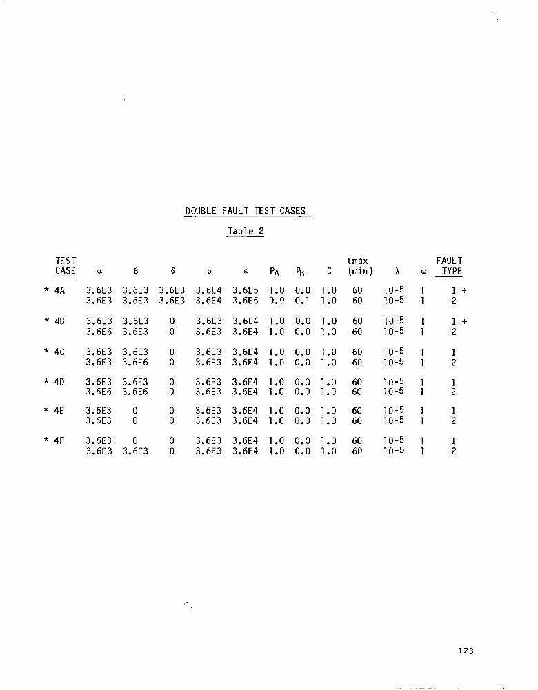
DOUBLE FAULT TEST CASES
Table 2
TEST tmax CASE a f3 6 P E PA PB C (min)
FAULT TYPE
1-k 2
x w
3.6E3 3.6E3
3.6E3 3.6E3
3.6E3 3.6E4 3.6E5 1.0 0.0 1.0 60 3.6E3 3.6E4 3.6E5 0.9 0.1 1.0 60
* 4A
* 4B
* 4c
* 4D
* 4E
* 4F
10-5 1 10-5 1
10-5 1 10-5 1
3.6E3 3.6E3 0 3.6E3 3.6E4 1 .O 0.0 1.0 60 3.6E6 3.6E3 0 3.6E3 3.6E4 1.0 0.0 1.0 60
1 + 2
3.6E3 3.6E3 0 3.6E3 3.6E4 1.0 0.0 1.0 60 3.6E3 3.6E6 0 3.6E3 3.6E4 1.0 0.0 1.0 60
10-5 1 10-5 1
1 2
10-5 1 10-5 1
10-5 1 10-5 1
3.6E3 3.6E3 0 3.6E3 3.6E4 1 .O 0.0 1.0 60 3.6E6 3.6E6 0 3.6E3 3.6E4 1.0 0.0 1.0 60 :
3.6E3 0 0 3.6E3 3.6E4 1.0 0.0 1.0 60 3.6E3 0 0 3.6E3 3.6E4 1.0 0.0 1.0 60
1 2
10-5 1 10-5 1
3.6E3 0 0 3.6E3 3.6E4 1.0 0.0 1.0 60 3.6E3 3.6E3 0 3.6E3 3.6E4 1.0 0.0 1.0 60
1 2
123

FTMP CASES
a
10
:o" 10
100 100 100 100
1000 1000 1000 1000
B
1
1:: 1000
1
1:: 1000
1
1;: 1000
Table 3
CARE III CARE III CARE III DRAPER PHASE III PHASE II PHASE I MODEL
1.1149 1.1161 1.124 1.2196 1.2041 1.207 1.1725 1.1682 1.1718 1.174 1.123 1.1274 1.129
0.9331 1.0054 1.2073 1.9527 1.9072 1.924 1.664 1.6585 1.661 1.215 1.2142 1.2181 1.220
0.263 0.2847 0.4239 1.46 3.387 3.3973 3.7975 4.22 6.3614 6.1513 6.17 2.156 2.1198 2.12
Failure Probability (x 10-8)
NOTE: Not all cases were run for Phase II.
124

SIFT CASES
Table 4
CARE III CARE III TEST Nl N2 X A 6 PHASE III PHASE I SRI
1 2
1 10 5 l.OE-4 l.OE-5 180 2.4858873E-8 2.4861769E-8 2.50 E-8
2 9 4 l.OE-4 l.OE-5 180 1,9880060E-8 1.988242lE-8 2.00 E-8
3 8 3 l.OE-4 l.OE-5 180 4.5428416E-8 4.5400324E-8 4.56 E-8
4 10 5 l.OlE-4 l.lE-5 18000 2.5373536E-10 2.5115lOlE-10 2.55 E-10
5 9 4 l.OlE-4 l.lE-5 18000 2.08176805E-10 2.0611656E-10 2.10 E-10
6 8 3 l.OlE-4 l.lE-5 18000 3.6450809E-8 3.6412602E-8 3.65 E-8
125

126

APPENDIX 1
Source Listings SFMODL DFMODL
127


PRCGRAM SF~ODL~~hPUT,OUTPUT,TAPE5=INPU7,TAPF6=OUTPUT,~LFIL~, 1 TAPE4=FLFILE)
C********************x*****~******X**************************** C THIS PROGKAY CALCULATES INTERMEDTATE FlJNCTTONS USED If; Ttit C THE SINGLE FAULT MCDEL 11J C0VRGE.w C********************~**********~*******************************~***
COMMON// SFAR(1ROO),IDlJBAR(YO),EIGAC4,4~,TI~EClROO~, 1 ITITLEC6),JTlTLEC6),PARClHOO,4)
COMMON/FLTPM/ ALPHA,HETA,DELTA,RHO,FF’SILON,PA,PU,C DIyENSION THASR(4) LOGICAL PFFLAG,GENXPTS,ANOTtiER,f’DPFLG,F’LTFLG,QFLAG COMMON/FIGCOM/ EIGSD(4,4,4),FIGVR(4) DATA A,NOTNER/.FALSE./,TBASK/5HHKS ,SHKINS ,SHSECS ,5HdSECS/ R 1. iJ I N D 4 PLTFLG = ,FALSF. ClRl TE (6;,9)
9 FORMAT (3X, “TYPF 8 REAL NUMbfiRS SEPAHATED f!Y COMMAS FOR “, 1 / I, PLPH.A,t~ETA,DELTA,RHO,tPSlLON,PR,C”)
kEAD(5,*) 4LFHA,YETA,GtLTA,RHO,FPSILON,PA,PE,C WRITE(6,55)
59 F(‘R!‘ATC/,3X, “TYPE AN INTEGtk mLE.4 FOR TIpmt BASE AS Ifq CAkt3”) RFADCS,*) ITGASF
30 l-‘RITEC6,31) GFLAG = .FALSF.
31 FORMAT (/,3X ,-ENTER F\It?CTIC:Y TO E!t CALCULATEC AS: ‘PA’,‘PH’,‘PNf!‘” 1 II ,‘PL’,‘PF’,‘PCP’,OR IQ'")
RFAD(5,32) FUNCTYP 32 FORI-‘AT(A3)
IFCFUhCTYP.Nt,3HGl > GO TO 33 URITF(6,34)
34 FORhAT (/,3X, “thTER FLIGHT TIME, F1UMPER OF ‘G’ STtPSC.LEm64)“) RF”DCS,*) FT,‘JOSTPS QFLAG = .TKUF. PFFLAG = .FALSC. FDPFLG = -FALSE. GI! TO 35
33 WKITEC6,40) 40 FORMAT C/,3X, “ENTER IHTTIAL STEP SIZt”)
READ C5,*) STEP STFPIN = STEP WRTTE(6,50)
50 FORMATC/,3X, “ENTEK DOUbLING ARRAY; DELIMIT \jITtl COMMAS.“,/) RFADC5,*) CIDUHAHCh),N=1,40) ITSTPS = 0 DO 51 N = 1,40
51 JTSTPS = .IDUBARCN) + JTSTPS ITSTPS = TTSTPS + 1 ICOEF = 0 PFFLAG = -FALSE. FDPFLG = -FALSE, PF = 0.0 GENXP-TS = -FALSE.
129

C C C
IFCFUliCTYP,ELi.3!iPA 1 IFUNCTN = 1 IF<FUNCTYP.EQ.3F!PP 1 IFUNCTN = 2 IF CFUNCTYP.EQ -3HPNB) IFUNCTN = 3 IFCFUNCTYP.EG.3HPL 1 IFUNCTN = 4 IFCFUNCTYP.EQ.3HPF 1 PFFLAG = -TRUE, IFCFUNCTYP.EQ.3HPDF) PDPFLG = .TRUF. INDEX=1 IFCIFlJNCTfi’.NF.O .OH. FFFLAG .OR, PDPFLG) GO TO 56 WRITEC6,55)
55 FORMAT (/,3X, “UNRECOGNIZED FUNCTION”) GO TO 30
56 NSTPST=l NSTFF=IDUEARCl) T=O.O IFCANOTHER) GO TO 25
CHOOSF. TIME BASE CONVERSION FACTOR
35 Tt3CF=O.D THASE=TOASHCTTBASE) IF CTBASE.EO,SHHRS 1 TRCF=l.O IF([email protected]’~JNS 1 TUCF=60.0 IF CTBASE .Ec,SHSFCS > TRCF=3600.0 IF CTBP.SE .EQ.SHMSECS) TRCF=3.6E6 IF(TPCF.NE.O.0) GO TO 17 WRITEC6.23) TBASE
23 FORKATC/“** CHRCR I~\:C~JRRECT TIME BASE = “,AE_) STOF
17 ALPHA=ALPHA/TPCF BETA=BETA/TGCF DELTA=DELTA/TGCF EPSILON=EPSILOK/THCF RRO=RHO/THCF
EIGACI,J) ARE THE ELFMLNTS OF THL MATRIX wt'1Cl-l REPRESFNTS THE CARE111 SIhGLE FAULT MCjDFL
18 EIGA(l,l) = -CALPHA+RI1O+FA*DELTA) EIGAC1,2) = PETA EIGAC1,3) = Cl-PA)*C*EPSILOB EIGAC1,4) = 0.0 EIGAC2,l) = ALPHA EIGA(2,2) = -BETA EIGAC2,3) = 0-O EIGA (2,4) = Cl-O-PG)*C*EPSILON EIGAC3.1) = RtiO FIGA(I,2) = 0.0 EIGA(3,'3) = -CALPHA+EPSILON) EIGA(3,4) = BETA EIGAC4,l) = 0.0 EIGAC4,2) = 0.0 EIGA(4,3) = ALPFiA EIGA (4,4) = -(RETA+EPSILON) CALL EIGEN CETGA) DO 20 1=1,4 EIGWRCI) = - EIGWRCI)
20 CC?NTJNUF
130

25 IF(UFLAG) CALL SFQ(SFAR,TIME,FT,lVUSTPS) IF(.NOT,FDPFLG) GO TO 22 CALL PDP(SFAR,TIML,STEF,ITSTFS,IDURAR) GO TO 75
22 IF(.NOT. PFFLAG) GO TO 60 DO 58 I=NSTFST,NSTPF
DC 57 L=1,4 IFCEIGiiRCL).EQ,O.OJ GO TO "7
26 Ff = CCCEIGSDC3,L,l)+LIGSDC4,L,l))/EIGVR(L)) 1 *(l-O-PRFfXP(-EIGUR(L)*T)))+PF
57 CONTINUF TIME(I) = T T=T + STEP PF = Cl-O-C)*EPSILON*PF
SFAR(I) = PF FF = 0.0
58 CONTINUE GO TO 71
60 IF(OFLAG) GO TO 74 DO 70 1 = NSTPST,NSTPF
GO 65 ICOEF = 1,4 TRC1=EIGSD(ICOEF,1,1)*PREEXPC-'CFIGWRCl)*T)) TKP2=EIGSDCICCEF,2, l)*FREEXFC-CElGWACi)+T)) TRb’3=EIGSb(ICCEF,3,1)*PRFEXP(-~FIGWR(’)*T1~ TRM4=EIGSDCICCEF,4,1)*PRFEXP(-(E16WR(4)+T~~ PAR CI,ICOEF )=TRMl+TRM2+TRM3+TRM4 IF(PAR~J,ICOEF).LT.O.0) PRRCI,ICOEF) = 0-O
65 COhT 1NUF TlFIE(I)=T T=T+STEP
70 CONTIN!JF 71 CONTINlJE
IYDEX=INDEX+l NSTPST=NSTPF+l NSTPF=NSTPST-l+IDURAR(IKDEX) STEP=STEP*2, IF(I.LF.ITSTPS) GO TO 25 IFtPFFLAG) GO TO 74 DO 73 I = 1,ITSTPS
PARtI, = PARCI,l) + PARCI,3) + PARtI, PARtI, = PAR(I,2? + PARtI, SFAR(I) = PAR(I,IFUNCTN)
73 CONTINUI! 74 CONTINUE 75 WRlTE (6,76) 76 FORMAT(/,3X;“UOULD YOU LIKE THIS ARRAY FRINTED AT THE TERMINAL ?"I
READ(5,lGl) IANStdER IFCIANSWER.NF.lHY) 60 TO 91 DO 90 I=l,ITSTPS
URITEC6,80) I,SFARCI),TIMECI) 80 F0RMATC/,3X,14,5X,E16.10,5X,1F'E16.10) 90 COkTIhiUE 91 CONTIhUE
131

WRITE (6,951 95 FOKF?AT (/,3X, “WOULD YOU LIKE THIS FUtiCTIOtJ PLOTTED ?“I
RFADCC,, 101) IANSWER IFCIANSk!ER.EQ.lHY) PLTFLG = -TRUE. IFCIANSWER.NE.lHY) GO TO 102 URITECG,96)
96 FORHATC/,3X, “ENTER PLOT TYPE: l=LINEAR, 2=LOG, 3=EOTH”) READ C5,*) LNORLG ENCODE (55,97,JTITLE) FUNCTYP
97 FORSATC9HFUNCTION ,A5,lH$) E~CODEC60,98,JTITLE) STEPJN,TBASC,ITSTPS
98 FORPATC2hHX AXIS WITH IFIIJIAL XSTFP= ,lPE6.2,A5, 1 13H PTS FLCTTEC=, 14,1H%)
CALL CPLOT~SfAR,TI~E,STEFI~,6ENXPTS,~TSTPS,LNORLG,ITITL~,JTITL~~ 102 WRITEC6,lOO) 100 FORF?AT C/,3X, “DO YOU WISH TO COMFUTE ANOTHER FUNCTIOk?“)
READCS, 101) IAYSWER 101 FORFAT
AKOTHFR = -TRUE. XFCJANSkER.EQ.ltiY) GO TO 30 IF CPLTFLG) CALL DOKFFL STOP FND FUMC JION PREEXP (X1
DATA hFALffAX/l.OE+322 /,KEAL~IN/l.OL-293/,EXPt?AX/741.67/, 3 EXPVIN/-675.821
IF CX.GT.EXPf-‘iIN .Pb.‘D. X.LT.EXPvAX) GO TO 100 C SET FUMCTION TO A VALUE VERY CLC’SE TO 0-O CiUT NOT EQUAL TO 0-C
IF (X,LE.EXPMIN) PKEEXP = RkALMIN C SET FUNCTION TO THE MAXIIYUM VALUE THF CDC CAN l!AtlDLE
IF CX.GE.EXPMAX) PRFEXP = REALKAX GO TO 200
100 PREEXP = EXPCX) 200 RETURN
E K D
132

SUBROUTINE PDPCPDPAR,TIME,STEP,ITSTPS,IDUBAR) COMMON/FLTPM/ ALPHA,DETA,DELTA,RHO,EPSILON,FA,PB,C DIMENSXON PDPAR(l),TIME(l),IDUEAR(l) INDEX = 1 NSTPST = 1 NSTPF = IDUBARCINDEX) T = 0.0 CNl = (2.0*ALPHA+RHO+EFSILON+PA*DELTA)/2.0 CN2 = SQRTCCRHO-EPSTLON+PA*DELTA)**2.0
1 +4.0*RHO*Cl-PA)*C*EPSILON)/2.0 RLAMl = CNl + CN2 RLAY2 = CNl - CN2 RLAM3=EPSILON IFCPA,EQ.l,O) GO TO 20 Al=CRLAM2-CALPHA.+RHO+PA*DELTA))/(RLAM2-HLAf’l1 A2=CRLAMl-CALPHA+RH!?+PA*DELTA))/CRLAMl-RLAY2) Pl=~~ALPHA+RH~+PA*CELTA-RLAM1)/((1,0-PA~~C*EPSILON~~~Al 62=((ALPHA+RHO+PA*DELTA-RLAM2)/((l.O-PA~*C*EPSILON))*A2 GO TO 40
20 IFCCRHO-EPSILON+DELTA).LT.O.O) GO TO 30 Al = 1.0 A2 = 0.0 Rl = -RHO/ (RHO-tPSILOK+DELTA 1 92 = -Bl GO TO 40
30 Al = 0.0 A2 = 1.0 Rl q RHO/CRHO-EPSILON+DELTA) 82 = -Rl
40 Cl=CALPHA/(EPSILON-RLAMl)J*Bl C2=CALPtIA/CEPSILON-RLAM2))*82 CONST1=PA*DELTA*A1+PA*C*EPSILON*B1+PR*C*EPSILON*Cl CO’~ST2=PA*DELTA*A2+PA*C~EPSILON*B2tPB*C*EPSILON*C2 CONST3=PR*C*EPSILON*(C1+C2)
c” MAIN CALCULATIONS C
50 DO 100 I=NSTPST,NSTPF PDPAR~I~=CONST1*<~1~O-PKEEXPo)/RL~~~~l~ + CONST2*((1.0-
1 PREEXPC-RLAM2*T))/RLAM2) - CONST3*CCl.O-PREEXPC-RLAM3+T))/ 2 RLAM3)
TIME(I)=T T=T+STEP
100 CONTINUE INDEX = I-NDEX + 1 NSTPST=NSTPF+ 1 NSTPF = NSTPST + IDUBARCINDEX) - 1 STEP = STEP * 2 IF(T.LF.ITSTPS) GO TC 50 RETURN END
133

C C C
C C C
C C C
C C C
. .~
SIJPROUTINE SFQCQAR,TIKE,FT,NSTEPS) COMMON/FLTPM/ ALPHA,BCTA,DELTA,HHO,EPSILON,FA,PB,C COMMON/EIGCOM/EIGSD~4,4,4~,EIGWRC4) DIMENSION QARCl),TIME(l),PFARC65),PFLAR(65) DATA RLA,MBDl/l.OE-021
TH’IS SURROUTINE GENERATES FINAL ‘Q’ VALUES.
STEP = FT/.NSTEPS ITSTPS = NSTEPS + 1
SET INITIAL KNOtiN CONDITIONS
PFPRCl)=O.O PFLARCl)=O.O QARCl)=O.O T=STEP TIME Cl )=O. 0
CALCULATE COEFFlCIENTS AND CONSTANTS
CONST=Cl.O-C)*EPSILON CDl= EIGSDC3,111)+EIGSDC4,1,1) CD2= EIGSDC3,2,1)+EIGSD(4,2,1) CD3= EIGSDC3, 3,1)+EIGSDC4,3,1) CD4= EIGSDC3,4,1)+EIGSDC4,4,1) Z 1 = EIGWR Cl)-RLAMBDl 22 = EIGWRC2)-RLAMBDl 13 = EIGURC3)-RLAMUDl 24 = EIGWRC4)-RLAMRDl
MAIN CALCULATIONS
DO 150 ITAU=2,ITSTPS Xl = -CEIGWRCl)*T) EIGLlT = 1.0 - PREEXPCXl) x2 = -(EIGWP(2)*T) EIGL2T = 1.0 - PREEXPCXZ) x3 = -CEIGWRC3)*T) EIGL3T = 1.0 - FREEXPCX3) x4 = -CEIGWRC4)*T) EIGL4T = 1.0 - PREEXPCX4) x5 = -CZl*T) EIGL5T = 1.0 - PREEXPCXS) X6 = -CZ2*T) EIGL6T = l-0 - PREEXFCX6) x7 = -CZ3*T) EIGL7T = 1.0 - PREE%PCX7) X6 = -CZ4*T) EIGLST = 1.0 - PREFXPCX8) PFARCITAU)=CONST*CCCCC1*EIGL1T)/EIGLlT~/EIGWRCl)~ + CCCD2*EIGL2T)/
1 EIGWHC2))+ CCCD3*EIGL3T)/EIGWRC3)) + CCCD4*EIGL4T)/ 2 EIGVRC4) 1)
PFLAK(ITAU)=CONST*CC(CD1*EIGLST)/Z1) + CCCD2*EIGL6T)/Z2) + 1 CCCD3*EIGL7T)/Z3) + CCCD4*EIGLST)/Z4))
QARCITAU)= PFAR CITAU)-PFLAR CITAU)*PREEXPC-RLAMBDl*TJ TIMECITAU)=T T=T+STEP
150 CONTINUE RETURN END
134

SUBROUTINE EIGEN (EIGA) C ********************tt*t*******f**t********* C EIGEN CALLS TWO IMSL SUBROUTINES--EIGRF 8 LEQT2F C EIGRF COMPUTES EIGENVALES AND EIGENVECTORS OF C THE MATRIX EIGAC1.J) C LEQT2F SOLVES THE LINEAR SYSTEM AX=Y, WHERE C THE COLUMNS OF A ARE THE EIGENVECTORS OF EIGA C AND Y IS AN M BY N MATRIX YHOSE COLUMNS ARE THE INDIVI- C DUAL RIGHT HAND SIDESCNON-HOMOGENOUS TERMS) C ********************tt*tt****~***********************
COMMON/EIGCOM/ EIGSD(4,4,4),EIGWR<4) DIMENSION WK<24),WKAREA<28),A(4,41,EICA<4,4~ COMPLEX W(4),ZC4,4)
C NE16 IS THE SIZE OF THE MATRIX WHOSE EIGENVALUES C WE ARE FINDING C 24(WK DIMENSION) IS OBTAINED BY MULT. NEI6+2 BY NE16 C 28tWKAREA DIMENSION) IS OBTAINED BY EVALUATING CNEI6**2)+3*NEfG
NEIG=4 M=4 IDGT=4 IJOB=Z DO 50 J=1,4 DO 50 1=1,4 EIGCCI,J)=O-
50 1FCI.EQ.J) EIGCCI,J)=l. CALL EI6RF(EI6A,NEIG,NEI6,IJOB,W,Z,NEI6,WK,IER~ IF<WK(l).LT.l.O)PRINT(6,*) "EIGRF PERFORMED WELL,IER =",IER IF(UK(l).GE.l.O)PRINT(6,*)"EIGRF PERFORMED SATISFACTORY,IER =“,EIR IF(WK(1).6T.100.O)PRINT~6,*) “EIGRF PERFORMED POORLY,IEH =“,EIR DO 60 I=l,NEIG EIGWR(I)=W(I) DO 70 J=l,NEIG EIGACI,J)=ZCI,J) IF(ABS(EIGA(I,J))mGT.l.OE-10) 60 T:O 65 EICA(I,J)=OeO
65 A<I,J)=EIGA(I,J) 70 CONTINUE 60 CONTINUE
CALL LEQT2F~A,M,NEIG,NEI6,EI6C,ID6T,UKAREA,IER~ DO 80 K=l,NEIG DO 80 I=l,NEIG DO 80 J=l,NEIG
C EIGSD(I,J,K) ARE THE CONSTANTS USED TO CONSTRUCT THE C PROBABILITY FUNCTIONS PCIIKCT)) - PROBABILITY THAT THE SYSTEM C IS IN STATE I AFTER STARTING IN STATE K.
'C EIGSDCI,J,K)=EIGA(I,J)*EIGC~J,K)
80 CONTINUE RETURN END
135

SUBROUTINE CPLOT(ARTOPLT,X,STEP,GENXPTS,NPTS,LNORLG,ITITLE, 1 JTITLE)
c **********************~******+**************************** C THIS ROUTINE UORKS UITH THE DISSPLA PLOTTING PACKAGE. C +*~*******i***********t*++********************************************* C NOTE - ARRAYS ‘ARTOPLT’ AND ‘X’ MUST BE OF THE SAME DIMENSION C IN -THE CALLING ROUTINE,
DIMENSION ARTOPLT(l),X(l),ITITLEo,JTITLE~l~ LOGICAL GENXPTS,AZROFLG,XZROFLG,AEPZFLG DATA XAXISMX/7.0/,YAXISMX/8.O/,XLEFT/2,25/,XRIGHT/4.75/,
11 YLOWER/6.50/,YUPPER/7.5O/,IFRAME/2/,XPOS/2.SO/,YPOSl/7.25/, 2 YPOS2/7.O/,YPOS3/6.75/,AZROFLG/.FALSE,/,XZROFLG/.FALSE./, 3 AEPZFLG/.FALSE./
IF(NPTS.EQ.1) 60 TO 25 K 0 IT&T = 1 IAXSTYP = LNORLG IF(.NOT.GENXPTS) 60 TO 15 DO 10 I=l,NPTS
10 X(1)=(1-l)*STEP 15 IF(X(l).EQ.O-0) XZROFLG = -TRUE.
IFtXZROFLG) X(l) = STEPIl0.0 XMTN=X(l) XMAX=X(NPTS) YNIN=ARTOPLTC 1) YMAX=ARTOPLT(l)
P
;*************TEST FOR ARRAY - PLOT TYPE COMPATABILITY************* C
DO 20 J=l,NPTS IF(X(J).LT.XMIN) XMIN = X(J) IF(ARTOPLT(J).EQ.O.O) K = K+l IF(ARTOPLTCJ).EU.O.O) AZROFLG = -TRUE. IF(.NOT.CAZROFLG.AND.CCJ.EQl.OR.~J.EQ.NPTS~~~~ 60 TO 19
IF(J.EQ.1) ARTOPLTCJ) = ARTOPLT(J+l)/lO.O IF(J.EQ,NPTS) ARTOPLT(J) = ARTOPLT<J-l)/lO.O YMIN = ARTOPLTCJ) AZROFLG = -FALSE.
19 IF CARTOPLT CJ 1 .LT.YMIN) YMIN = ARTOPLTCJ) IF(ARTOPLT<J).GT.YMAX) YMAX = ARTOPLT(J)
20 CONTINUE IF(K.NE.NPTS) GO TO 31
25 WRITE (6,301 30 FORMAT(/4X, “ARRAY TO BE PLOTTED IS IDENTICALLY ZERO: NO PLOT”)
1 “GENERATED .“I RETURN
31 IF(.NOT.AZROFLG) 60 TO 33 WRITE (6,321
32 FORMAT(/4X, “DATA PCINT ON LOG AXIS .LE. ZERO; LINEAR”, 1 ” AXIS PLOT GENERATED,“)
IAXSTYP = 1 33 YTEST = CDm05*YMAX) + (0.95fYMIN)
XTEST = (Om05*XMAX) + (0.95*XMIN) NP = NPTS - 1 DO 34 I = 1,NP
IF(<XTEST.GE,X(I)),AND,(XTEST.LE,X(I+1))~ ITEST = I+1 34 CONTINUE
136

IF(ARTOPLT(ITEST),LE.YTEST) IAXSTYP = 4 IFtIAXSTYP .EQ. 4) WRITE (6,351
35 FORMATC/4X, “LINEAR PLOT INADEQUATE; LOG-LOG PLOT USED”) IF(XZROFL6) URITEC6.36) XMIN
36 FORMAT(/4X, “ZERO VALUE IN TIME ARRAY; XMIN = “,El0.5,” USED”) IFCAEPZFLG) URITE(6,37) YMIN
37 FORMAT(/4X, “ZERO VALUED END-POINT IN DATA: YMIN = “,El0.5, 1 ” USED FOR LOG PLOTS.“)
~**********+DIssPLA INITIALIZATION+**t*+*~**************~********** C
CALL COMPRS CALL BGNPLC-1) CALL NOCHEK IF(.AZROFLG) 60 TO 38 CALL ALGPLT(YMIN,YMAX,YAXISMX,YORIGL,YCL) CALL ALGPLT(XMIN,XMAX,XAXISRX,XORI6L,XCYCL~
38 CALL AXSPLT(YMIN,YMAX,YAXISMX,YORI6,YSTEP,YAXIS~ CALL AXSPLT(XMIN,XMAX,XAXISMX,XORIG,XSTEP,XAXIS)
C C********+*tLIHEAR PLOT ROUTINE*************+**********+****~***~****** C
IF(IAXSTYP.NE.l.AND.IAXSTYP.NE.3) GO TO 40 CALL TITLECITITLE,l00,JTITLE,lOO,"LINEAR Y-AXISS",lOO,
1 XAXISMX,YAXISMX) CALL FRAME CALL BLNKl(XLEFT,XRIGHT,YLOWER,YUPPER,IFRAME) CALL GRAPH(XORIG,XSTEP,YORIG,YSTEP) CALL GRID(l,2)
GO TO 50
~*****+***+*SEMI-LOG PLOT ROUTINE+***++****++*******+**************** C
40 IF(IAXSTYP.NE.2.AND.IAXSTYP.NE.3) 60 TO 45 CALL TITLECITITLE,l00,JTITLE;lOO,"LOC Y-AXISS",lOO,
1 XAXISf'X,YAXISMX) CALL FRAME CALL BLNKl(XLEFT,XRI6HT,YLOWER,YUPPER,IFRAME) CALL YLOG(XORI6,XSTEP,YORI6L,YCYCL~ CALL GRID<l,l)
GO TO 50 C Cf+t****+***L()6-L06 PLOT ROUTTNEt*********+*******+*****************~ C
45 IF<IAXSTYP.NEw4) GO TO 50 CALL TITLE<ITITLE,l00,JTITLE,lOO,"LOG-LOG PLOTs",lOO,
1 XAXISMX,YAXISMX) CALL FRAME CALL BLNKl(XLEFT,XRIGHT,YLOWER,YUPPER,IFRAME) CALL LOGLOGCXORIGL,XCYCL,YORIGL,YCYCL) CALL GRID(l,l)
C C***************~t*************************~*********************** C
137

50 CONTINUE C CALL DASH
CALL PESET(“BLNK1”) CALL MESSAG(“CARE III PROJECTS",lOOrXPOS,YPOS1) CALL MESSAG(‘*RAYTHEON COMPANYS”,&OO,XPOS,YPOS2) CALL MESSA6<“SUDBURY,MAS.SS”,lOO,XPOS,YPOS3)
C CALL RESET ("DASH") CALL CURVE(X,ARTOPLT,NPTS,O) CALL ENDPL (0) TFtIAXSTYP.NE.3) 60 TO 100 IAXSTYP = 2 60 TO 40
100 CONTINUE RETURN END
138

PROGRAM DFMODL (INPUT,OUTPUT,TAPES=INPUT,TAPE6=OUTPUT, 1 PLFILE,TAPE$=PLF ILE 1
C C****************t*****************************************************~ c* l
c* THIS PROGRAM ANALYTICALLY CALCULATES THE INTERMEDIATE l
c* DOUBLE FAULT FUNCTION PDF, FOR COMPARISON WITH CARE III. l
c* *
C*********************************************************************~*
C
C C C C C C C C C C C C C C C C C C C C C C
COMMON// DFAR~l800~,IDUBAR~40~,TIME~l8OO~,ITITLE~6~,JTITLE~6~ LOGICAL GENXPTS,ANOTHER COMMON/DEI6COM/DEIGSO~3,3,3~,DEIGWR~3~,DEI6A~3,3~,NEIGD,
1 DEIGTC(3) DIMENSION FLTPM(9,2),EVALDF(4,2),COEFDF(4,4,4,2~,TBASRC4~ DATA TBASR/SHHRS ,SHMINS ,SHSECS ,SHMSECS/,ANOTHER/.F./
INPUT PARAMETERS
THE FAULT TYPE PARAMETERS ARE STORED IN THE ARRAY: FLTPM(I,L),
I PARAMETER ------------- 1 * ALPHA 2 * BETA 3 * DELTA 4 * RHO 5 * EPSILON 6 * PA 7 * PB 8 l C
9 * LAMBDA
L PARAMETER ------------- 1 * FIRST FAULT TYPE 2 * SECOND FAULT TYPE
REWIND 4 WRITE(6.10)
10 FORMATC3X,/, “ENTER FIRST FAULT TYPE PARAMETERS AS FOLLOWS: “,I, 16X, “ALPHAl,BETAl,DELTAl,RHOl,EPSILONl,PAl,PBl,Cl”~
READCS,*) <FLTPMC1,1),1=1,8) WRTTE<6,15)
15 FORMATt3X.1, “ENTER SECOND FAULT TYPE PARAMETERS AS FOLLOWS:. “,/, 16X, “ALPHA2,BETA2,DELTA2,RHO2,EPSILON2,PA2,PB2,C2”)
READ(S,*) (FLTPM(1,2),1=1,8) WRITE(6,20)
20 FORMAT(/,3X, “TYPE AN INTEGER -LE.4 FOR TIME BASE AS IN CARE3”) READ <5,*) ITBASE
139

25 WRITE (6,301 30 FORMAT (/,3X, “ENTER ITYP,JTYP:‘)
READ(S,*) ITP,JTP WRITE<6,40)
40 FORMAT(/,3X, “TYPE AN INTEGER .LE. 1799 FOR NUMBER OF STEPS”) READ (5,*) ITSTPS WRITE (6,451
45 FORMAT </,3X, “ENTER INITIAL STEP SIZE”) READC5,*) STEP STEPIN = STEP WRITE(6,50)
50 FORMAT(/,3X, “ENTER DOUBLING ARRAY; DELIMIT WITH COMMAS.“,/) READ(5,*) (IDUBARCN),N=l,YO) ITSTPS = ITSTPS + 1 GENXPTS = -FALSE. INDEX=1
60 NSTPST=l NSTPF=IDUBAR(l) T=O.O
c
; CHOOSE TIME BASE CONVERSION FACTOR C
IFtANOTHER) 60 TO 76 TBCF=O.O TBASE=TBASR<ITBASE) IFCTBASE .EQ .SHHRS 1 TBCF=l.O IFCTBASE.EQ.SHMINS 1 TBCF=60.0 IF(TBASE.EQ.5HSECS 1 TBCF=3600.0 IF(TBASE.EQ.5HMSECS) TBCF=3.6E6 IF(TBCF.NE.O.0) 60 TO 69 WRITE(6,65) TBASE
65 FORMAT(/“** ERROR INCORRECT TIME BASE = “,A51 STOP
69 DO 75 L=l,2 DO 70 1=1,5
FLTPM(P,L) = FLTPM(I,L)/TBCF 70 CONTINUE 75 CONTINUE 76 CONTINUE
140

C C -------------DOUBLE FAULT MATRIX CALCULATIONS -------------------------- C C EVALDF(I,L) =E.IGENVALUES (LAMBDAl.. -LAMBDA21 C COEFDF(I,J,L)=CHARACTERISTIC EQUASION COEFFICIENTS. C L-INDEX=INITIAL CONDITION Cl OR 2) C J-INDEX=EQUASION A,B,C,OR D <1,2,3,OR 4) C I-INDEX=COEFFIClENT I.E. AlrA2,A3,0R A4 C C EIGA(I,J) ARE THE ELEMENTS OF THE MATRIX WHOSE C EIGENVALUES WE ARE FINDING. L
NEIGD=3 C C SET INITIAL CONDITIONS C
DEIGIC (l)=l DEIGIC C2)=0 DEIGIC(3)=0 DO 90 L=l,2 DEIGA(l,l) =-(FLTPM(l,JTP)+FLTPM(2,ITP)+FLTPM(4,JTP)+FLTPM(3,JTP)) DEIGA (1,2)=FLTPM(2,JTP) DEIGA (1,3)=0.0 DEIGA (2,l)=FLTPM<l,JTP) DEIGA(2,2) =-<FLTPMC2,ITP)+FLTPMC2,JTP)1 DEIGA<2,3)=FLTPM(l,JTP) DEIGA<3,1)=0.0 DE IGA (3,2)=FLTPMC2, ITP) DEIGA (3,3)=- (FLTPM(l,ITP)+FLTPM(2,JTP)+FLTP~(4,ITP)+FLTPM(3,ITP))
CALL DEIGEN DO 85 J=l,3
EVALDFCJ,L)=-DEIGWRCJ) DO BO 1=1,3
IF(L.EQ.1) K = 1 IF(L.EQ.2) K = 3 COEFDF(I,J,L)=DEIGSD<J,I,K)
80 CONTINUE 85 CONTINUE
DEIGIC(l)=O DEIGIC(3)=1
90 CONTINUE FUNCTYP = 3HPDF
120 DO 135 I = NSTPST,NSTPF DFARCI) = 0.0 RHO1 = FLTPMC4, TTP) l PREEXPC-FLTPMC4,ITP)*T) RHO2 = FLTPMC4,JTP) * PREEXPC-FLTPM(4,JTP)*T) BETA1 = FLTPM (2,ITP) BETA2 = FLTPM(2,JTP)
PA182 = 0.0 PA2Bl = 0.0 DO 125 N = 1,3
PAlBP = (COEFDF(N,3,l)*PREEXP(-EVALDFCN,l>*T.))+PAlf32 PA2Bl = (COEFDFCN,l,l)*PREEXP(-EVALDF(N,1)*T))+PA2Bl
125 CONTINUE DFAR(I) = ((BETA2+RHOl)*PAlB2)
1 + C(BETAl+RH02)*PA2Bl) TIME(I) = T T = T + STEP
135 CQNTINUE
141

INDEX = INDEX + 1 NSTPST = NSTPF + 1 NSTPF = NSTPST + IDUBARCINDEX) - 1 STEP = STEP * 2 IFCI .LE. ITSTPS) 60 TO 120 WRITE<6,140)
140 FORMAT(/,3X, “WOULD YOU LIKE THIS ARRAY PRINTED AT THE TERMINAL 7”) READ(5,lOl) IANSWER IF(IANSUER.NE.lHY) GO TO 155 URITE(6,142) FUNCTYP,ITP,JTP
142 FORMAT(lHl,/,3X,“FUNCTION “,A3,” ITYP= “,12,” JTYP= “,I21 DO 150 I=l,ITSTPS
WRITE(6,145) I,OFAR(I),TIMECI~) 145 F0RMAT(/,3X,14,5X,E16.10,5X,1PE16.10) 150 CONTINUE 155 CONTINUE
WRITE(6,160) 160 FORMAT(/,3X, “WOULD YOU LIKE THIS FUNCTION PLOTTED ?“I
READ(5,lOl) IANSWER IF<IANSVER.NE.lHY) GO TO 176 WRITE(6,165)
165 FORMATC/,SX, “ENTER PLOT TYPE: l=LINEAR, 2=LCG, 3=BOTH”) READCS,*) LNORLG ENCODEC55,170,ITITLE) FUNCTYP,ITP,JTP
170 FORMATCSHFUNCTION ,A5,7H ITYP= ,13,7H JTYP= ,I3,lHS) ENCODEC60,175,JTITLE) STEPIN,TBASE,ITSTPS
175 FORMAT(26HX AXIS WITH INITIAL XSTEP= ,lPE8,2,A5, 1 13H PTS PLOTTED=,I4,lHS)
CALL CPLOT~DFAR,TIME,STEPIN,6ENXPTS,ITSTPS,LNORL6,ITITLE,JTITLE~ 176 WRITE(6,180) 180 FORMAT(/,3X, “WOULD YOU LIKE TO COMPUTE ANOTHER FUNCTION?“)
READ(5,lOl) IANSWER IF(IANSWER.EQ.lHY) ANOTHER = -TRUE. IFCIANSWER.EQ.lHY) GO TO 25
101 FORMAT 190 CONTINUE'
CALL DONEPL STOP END FUNCTION PREEXPCX)
C DATA REALMAX/l.0E+322/,REALMIN/l.OE~293/,EXPMAX/74l.67/,
1 EXPMIN/-675.821 C
IF (X .GT .EXPMTN .AND. X.LT.EXPMAX) 60 TO 100 C SET FUNCTION TO A VALUE VERY CLOSE TO 0.0 BUT NOT EQUAL TO 0.0
IF (X.LE.EXPMIN) PREEXP = REALMIN C SET FUNCTION TO THE MAXIMUM VALUE THE CDC CAN HANDLE
IF (X.GE.EXPMAX) PREEXP = REALMAX 60 TO 200
100 PREEXP = EXPCX) 200 RETURN
FNh
142

SUBROUTINE DEIGEN C ************************************************ C DEIGEN CALLS TWO IMSL SUBROUTINES--EIGRF & LEQT2F C EIGRF COMPUTES EIGENVALES AND EIGENVECTORS OF C THE MATRIX EIGA<I,J) C LEQT2F SOLVES THE LINEAR SYSTEM AX=Y, WHERE C THE COLUMNS OF A ARE THE EIGENVECTORS OF EIGA C AND Y IS AN M BY N MATRIX WHOSE COLUMNS ARE THE INDIVI- C DUAL RIGHT HAND SIDESCNON-HOMOGENOUS TERMS) C ****************************************~******~*
COMMON/DEIGCOM/ EI6SD(3,3,3),EI6WRC3),EI6A~3,3~,NEI6,EI6IC~3~ DIMENSION WK<l5),WKAREAClR),AC3,3~,EIGCC3,3) COMPLEX ‘d(3),2(3,3)
C NE16 IS THE SIZE OF THE MATRIX WHOSE EIGENVALUES C WE ARE FINDING C 15CWK DIMENSION) IS OBTAINED BY MULT. NEI6+2 BY NE16 C 18tldKAREA DIMENSIGN) IS OBTAINED BY EVALUATING CNEIG**2)+3*NEIG
M=NEIG IDGT=4 IJOB= DO 50 J=l,NEIG DO 50 I=l,NEIG EIGC(I,J)=O.
50 1FCI.EQ.J) EIGCCI,J)=l. DO 55 I=l,NEIG
EI6C(I,l)=EIGIC(I) 55 CONTINUE
CALL EIGRF(EI6A,NEI6,NET6,IJOf3,W,Z,NEI6,WK,IER~ IF(WK(l).LT.l.O)PRINT(6,*) “EIGRF PERFORMED WELL,IER =",IER IF(WK(1).6E.l.O)PRINT~6,*~"EI6RF PERFORMED SATISFACTORILY, =“,
1IER IF(WK(l).GT.l00.O)PRINT(6/*) I'EIGRF PERFORMED POORLY,IER =",IER DO 60 I=l,NEIG EIGURCI)=W(I) DO 70 J=l,NEIG EIGA(I,J)=Z(I,J) IF(ABSCEI6A<I,J)).6T.l.OE-10) GO TO 65 EIGA(I,J)=O.O
65 A<I,J)=EIGA(I,J) 70 CONTINUE 60 CONTINUE
CALL LEQT2F~A,M,NEIG,NEI6,EIGC,IDGT,WKAREA,IER~ DO 80 K=l,NEIG DO. 80 I=l,NEIG DO 80 J=l,NEIG
C EIGSD<I,J,K) ARE THE CONSTANTS USED TO CONSTRUCT THE C PROBABILITY FUNCTIONS P<I/K(T)) - PROBABILITY THAT THE SYSTEM C IS IN STATE I AFTER STARTING IN STATE K.
EI6SD~I,J,K)=EIGA~I,J)+EIGCo C C
80 CONTINUE RETURN END
143

SUBROUTINE CPLOT(ARTOPLT,X,STEP,6ENXPTS,NPTS,LNORL6,ITITLE, 1 JTITLE)
c ****f***********.****t*******************************************~~******* C THIS ROUTINE WORKS WITH THE DISSPLA PLOTTING PACKAGE. c ****t*******t*******************************************************~ C NOTE - ARRAYS ‘ARTOPLT’ AND ‘X’ MUST BE OF THE SAME DIMENSION C IN THE CALLING ROUTINE.
DIMENSION ARTOPLT(l),X~l),ITITLE~l~,JTITLEO LOGICAL GENXPTS,AZROFLG,XZROFLG,AEPZFLG DATA XAXISMX/7.0/,YAXISMX/8.O/,XLEFT/2.25/,XRIGHT/4.75/,
1 YLOUER/6.50/,YUPPER/7.5O/,IFRAME/2/,XPOS/2.5O/,YPOSl/7.25/, 2 YPOS2/7.O/,YPOS3/6.75/,AZROFLG/,FALSE./,XZROFL6/.FALSE./, 3 AEPZFLG/.FALSE./
IF<NPTS. EQ.1) 60 TO 25 K 0 IT&T = 1 IAXSTYP = LNORLG IF(.NOT.GENXPTS) 60 TO 15 00 10 I=l,NPTS
10 X(1)=(1-l)*STEP 15 IF(X(l).EQ.O.O) XZROFLG = -TRUE.
IFtXZROFLG) X(l) = STEP/IO.0 XMIN=X(l) XMAX=X CNPTS) YMIN=ARTOPLT (1) YMAX=ARTOPLTCl)
r
~**+***++*****TEsT FOR ARRAY - PLOT TYPE COMPATABILITY************* C
DO 20 J=l,NPTS IF(X(J).LT.XMIN) XMIN = X(J) IF(ARTOPLT*CJ).EQ.O.O) K = K+l IF(ARTOPLT(J).EQ.O.O) AZROFLG = -TRUE. IF(.NOT.CAZROFLG.AND,((J,EQ.l~.OR.CJ.EQ.NPTS1~1~ GO TO 19
IF(J.EQ.1) ARTOPLTCJ) = ARTOPLT(J+l)/lO.O ;;;;.EP.NPTS) ARTOPLTCJ) = ARTOPLT (J-1)/10.0
= ARTOPLT(J) AZROFLG = -FALSE.
19 IFCARTOPLTCJ) .LT.YMIN) YMIN = ARTOPLTCJ) IF (ARTOPLT (J) .GT.YMAX) YMAX = ARTOPLTCJ)
20 CONTINUE IFCK.NE.NPTS) GO TO 31
25 WRITE(6,30) 30 FORMAT(/4X, “ARRAY TO BE PLOTTED IS IDENTICALLY ZERO; NO PLOT”.,
1 “GENERATED.“) RETURN
144

31 IFC.NOT.AZROFLG) GO TO 33 URITE (6,321
32 FORMATC/4X, “DATA POINT ON LOG AXIS .LE. ZERO; LINEAR”, 1 ” AXIS PLOT GENERATED,“)
IAXSTYP = 1 33 YTEST = <Om05*YMAX) + (0.95*YMIN)
XTEST = (0,05*XMAX) + <O.SS*XMIN) NP = NPTS - 1 DO 34 I = 1,NP
IFCCXTEST.GE.XCI)).AND.(XTEST.LE.Xo)~ ITEST = I+1 34 CONTINUE
IFCARTOPLTCTTEST).LE.YTEST) IAXSTYP = 4 IFtIAXSTYP .EQ. 4) WRITE(6,35)
35 FORMATC/4X,“LINEAR PLOT INADEQUATE; LOG-LOG PLOT USED”) IFCXZROFLG) URTTEC6,36) XRIN
36 FORMAT</4X, “ZERO VALUE IN TIME ARRAY; XMIN = ",ElO.5," USED”) IFCAEPZFLG) WRITEC6.37) YMTN
37 FORMAT(/YX, “ZERO VALUED END-POINT IN DATA; YMIN = “,E10.5, 1 ” USED FOR LOG PLOTS.“)
E+**********DISSPLA INITIALIZATION**+*+***********+*****~************ C
CALL COMPRS CALL B6NPL C-1) CALL NOCHEK IFCAZROFLG) GO TO 38 CALL ALGFLT(YMIN,YMAX,YAXISMX,YORIGL,YCYCL) CALL ALGPLTCXMIN,XMAX,XAXISMX,XORIGL,XCYCL)
38 CALL AXSPLTCYMIN,YMAX,YAXISMX,YORTG,YSTEP,YAXIS~ CALL AXSPLT(XMIN,XMAX,XAXISMX,XORIGiXSTEP,XAXIS)
L
IFCIAXSTYP.NE.l.AND.IAXSTYP~NE.3) GO TO 40 CALL TITLE~ITITLE,100,JTITLE,lOO,“LINEAR Y-AXISS",lOO,
1 XAXISCX,YAXISMX) CALL FRAME CALL BLNK1<XLEFT,XRIGHT,YLOWER,YUPPER,YUPPER,IFl?AME~ CALL GRAPHCXORIG,XSTEP,YORIG,YSTEP) CALL GRIDC1.2)
GO TO 50 . ~*********+*sEMI-LOG PLOT R~ufx~Et+*********t+********************* c
40 IF.CIAXSTYP;NE.2.AND.IAXSTYP.NE.3) GO TO 45 CALL TITLECITITLE,100,JTITLE,lOO,“LOG Y-AXISS",lOO,
1 XAXISMX,YAXISMX) CALL FRAME CALL BLNKlCXLEFT,XRIGHT,YLOWER,YUPPER,IFRAME) CALL YLOGCXORIG,XSTEP,YORIGL,YCYCL) CALL GRID<l,l)
GO TO 50
145

C C,**+*tl****LoG-L()G PLOT ROUTINE**t*+*t****+*******~**+** C
45 IF(IAXSTYP.NE.4) GO TO 50 CALL TITLE(ITITLE,100,JTITLE,lOO,"LOG-LOG PLOTS",lOO,
1 XAXISMX,YAXISWX) CALL FRAME CALL BLNKlCXLEFf,XKIGHT,YLOWER,YUPPER,IFRAME) CALL LOGLOGCXORIGL,XCYCL,YORIGL,YCYCL) CALL 6RID(l,l)
L C**********t******t******+*****************************~**~*********** C
50 CONTINUE C CALL DASH
CALL RESET (“BLNKl”) CALL MESSAGC”CARE III PROJECTS”,100,XPOS,YPOS1) CALL MESSAG<“RAYTHE.ON COMPANYS”,lOO,XPOS,YPOS2) CALL MESSAGC”SUDBURY,CASSS”,lOO,XPOS,YPOS3)
C CALL RESETC”DASH”) CALL ClJRVECX,ARTOPLT,NPTS,O) CALL ENDPL CO) IFCIAXSTYP.NE.31 GO TO 100 IAXSTYP = 2 GO TO 40
1'00 CONTINUE RETURN END
i46

APPENDIX 2
Execution Field Lengths
PROGRAM FIELD LENGTH (Octal) A--
CAREIN ............................................................ 154000
COVRGE ............................................................ 163700
CARE3 ............................................................. 157200
CVGPLT ............................................................ 127600
RELPLT ............................................................ 076000
147
I

t

APPENDIX 3
Select&d Test Cases
149
I -


THE FOLLOYING ARE THE CARE111 INPUT FILES FOR THE SELECT TEST CASES REPORTED ON.
SFLTTYP ALP=O.,BET=O., DEL=3.6E3,RHO=3.6EY,EPS=3.6E5,IEPSF=l,IDELF=l, CVPLOT=.T .,IAXSCV=3,C=l,O,CVPRNT=.T.S
SSTAGES NOP=3,2,N=4,M=2,IRLPCD=31RLPLOT=,T.,IAXSRL=3S SFLTCAT OMG=l.O,RLM=l.OE-5 S SRNTIME FT=60., ITBASE=2,SYSFLG=.T.,CPLFL6=.T.,NSTEPS=64!&
***TEST CASE-TlA S-NEUMANN 23FEB82*** 1122 201 CRITICAL-FAULT TREE 1455 114 521234
SFLTTYP ALP=3.6E2,BET=O., DEL=O.O,RHO=3.6E4,EPS=3.6ES,IEPSf=1,IDELF=l, CVPLOT=.T .,IAXSCV=4,C=1.01CVPRNT=.T.,DBLDF=.06S
%STAGES NOP=3,2,N=4,M=2,IRLPCD=3,RLPLOT=,T.,IAXSRL=4$ SFLTCAT OM6=1-O,RLM=l.OE-5 S JRNTIME FT=60.,ITBASF=2,SYSFLG=.T.,CPLFLG=.T.,NSTEPS=64$
***TEST CASE-T2C S.NEUMANN 24FEB82*** 112 2 201 CRITICAL-FAULT TREE 1455 1 14 521234
%FLTTYP ALP=3.6Eb,BET=3~6E6,DEL=3.6E4,RHO=3.6E3,EPS=3.6E4,IEPSF=l, IDELF=2,CVPLOT=.T., IAXSCV=4,C=l.O,CVPRNT=.T.,DBLDF=.O2S
SSTAGES NOP=3,2,N=4,M=2,IRLPCD=3,RLPLOT=.T.,IAXSRL=4S ZFLTCAT OMG=l.O,RLM=l.OE-5 S SRNTIME FT=60 .,TTBASE=2,SYSFLG=.T.,CPLFLG=.T.,NSTEi’S=64S
***TEST CASE-TJB S-NEUMANN 24FEB82*** 112 2 2 0 1 CRITICAL-FAULT TREE 1455 114 521234
SFLTTYP ALP=3.6E3,RET=3,6E6,DEL=O~O,RHO=3.6E3,EPS=3.6E4,IEPSF=l,IDELF=l, CVPLOT=.T., IAXSCV=3,C=l.O,CVPRNT=.T.,TRUNC=I.OE-6f
SSTAGES NOP=3,2,N=4,M=2,IRLPCD=SIRLPLOT=,f .,IAXSRL=3S JFLTCAT OMG=l.O,RLM=l.OE-5 S SRNTIME FT=60 .,ITBASE=2,SYSFLG=.T.,CPLFLG=.Te,NSTEPS=64$
***TEST CASE-T3C S.NEUMANN 02MAR82*** 1122 201 CRITICAL-FAULT TREE 1455 114 521234
g-l----------------------------- -r--II-r-------r--r-------------------.
151

SFLTTYP ALP=3.656,RET=3-6E3,DEL=3.6E4,RHO=3.6E3,~PS=3.6E4,IEPSF=l, IDELF=2,CVPLOT=,T., TAXSCV=4,C=l,O,CVPRNT=.T,,DBLDF=0.02S
SSTAGES NOP=3,2,N=Y,M=2,IRLPCD=3,RLPLOT=.T.,TAXSRL=4S SFLTCAT OMG=l.O,RLM=l.OE-5 f SRNTIME FT=60., ITBASE=2,SYSFLG=.T.,CPLFLG=.T.,NSTEPS=64$
***TEST CASE-T3D’ S-NEUMANN lMAR82*** 112 2 201 CRITICAL-FAULT TREE 14 5 5 114 521234
SFLTTYP ALF=2*3.6E3,EET=2*3,6E3,DEL=2*3.6E3,RHO=2*3.6~4,EPS=2*3.6E5, NFTYPS=2,IEPSF=2*1,IDELF=2fllCVPLOT=.T.,IAXSCV=3,C=l.O,CVPR~~T=.T.,
PA=l.O,O.9,PH=D.O,0~1 S tSTAGES NOP=3,2,%=4,M=2,IRLPCD=3,RLPLOT=.T,,IAXSRL=3S IFLTCAT OMG=l.O,RLM=l,OE-5 S %RNTTME FT=60., ITBASE=2,SYSFLG=.T.,CPLFLG=.T.,NSTEPS=64$
***TEST CASE-T4A S-NEUMANN 031MAR82*** 112 2 201 CRITICAL-FAULT TREE. 1455 114 521234
fFLTTYP ALP=3-6E3,3.6E6,RET=2*3.6E3,DEL=2*O.O,RH~=2*3-6E3,~PS=2*3.6E4, NFTYPS=2,IEPSF=2*1,IDELF=2*l,CVPLOT=.T.,IAXSCV=3,C=l.O,CVPR~T=.T., PA=2+l.O,Pf3=2*0.0 $ SSTA6ES NOP=3,2,N=4,M=2,IRLPCD=3,RLPLOT=.T.,TAXSRL=3$ SFLTCAT OMG=l .O,RLM=l.OE-5 S SRNTIME FT=60 .,ITBASE=2,SYSFLG=.T.,CPLFLG=.T.,NSTEPS=64$
***TEST CASE-T48 S.NEUMANN 02YAR82*** 112 2 201 CRITICAL-FAULT TREE 1455 114 521234
---------------------------------------------------------------------------~
152

APPENDIX 4
Coverage Functions
153


Single-Fault Model Equations
FUNCTION MATHEMATICAL EXPRESSION* DEFINITION I
4 (t)
p,(t)
6-l TIMES THE PROBAB I LITY INTENSITY OF RE-ENTERING STATE A EXACTLY t TIME UNITS AFTER THE PREVIOUS ENTRY
-at t PROBABILITY OF BEING IN e r(t)d(t) + 8 Ut-r)Pah)dT STATE A AT TIME t WHEN
0 PA = PB = 1
t PROBABILITY OF BEING IN 44q + B STATE B AT TIME t WHEN
0 $(t-T)P$)dT
PA = PB = 1
pa (t1
pe (t) t t PROBABILITY OF BEING IN
e -aTp(r)d(r)e(t-r)dT t fj 0 0
4(t-T)Pe(r)dr STATE AE OR BE AT TIME t WHEN PA = pB = 1
=I l t HERE IS A MEASURE OF THE TIME SINCE THE ENTRY INTO STATE A, VI

Single-Eault Model Equations(Continued)
FUNCTION MATHEMATICAL EXPRESSION* DEFINITION
p,(t)
P,W
PfW
yt1
t e -atdt)d(tl + 8 o 44t-T)pe(f)dT
s t e -at6(t)r(t) + 8 o ~(t-T)P$M
t (1-C)
0 pe(rkWW
t (t-T) C
0 PehMt-T) dt f p,(t)
INTENSITY OF ENTRY INTO STATE AE AT TIME t WHEN PA = PB = .l
INTENSITY OF ENTRY INTO STATE AD FROM STATE A’AT
TIME t WHEN PA = PB = 1
INTENSITY OF ENTRY INTO STATE F AT TIME t WHEN P* = PB = 1
INTENSITY OF ENTRY INTO STATE AD AT TIME t FOR, THE FIRST TIME
l t HERE IS A MEASURE OF THE TIME SINCE THE ENTRY INTO STATE Aa

Single-Fault Model Equations(Continued)
FUNCTION MATHEMATICAL EXPRESSION* DEFINITION
yg (a aC 5 t a+B 0 Pe(T) (1 - e'(a+B)(t'r)),(t-T)dT
XB (t)
PdpW
' t
I YB(t)e -6 ($-?I dt
! 0
t pA o '$+)aT + PB
t F,(t) Fx(t) + 0
t(l-PA)rA(t-T) + (1.P,)BX,(t-~)]F,[T)dr:
INTENSITY OF ENTRY INTO
STATE B. AT TIME t FOR
THE FIRST TIME
PROBABILITY OF HAVING
ENTERED STATE BD FOR THE
FIRST TIME AND THEN RE-
MAINING IN THE BENIGN
STATE UNTIL TIME t
PROBABILITY THAT A FAULT
HAS BEEN DIAGNOSED AS
PERMANENT BY TIME t
FUNCTION RELATING PROB:
ABILITIES AND INTENSITIES
DERIVED WHEN ‘A = pB = 1 TO
THOSE SAME QUANTITIES WHEN
PA h pB ARE ARBITRARY
rl 4 l t HERE IS A MEASURE OF THE TIME SINCE THE ENTRY INTO STATE Am

Single-Fault Model EqUatiOllS~Continued
FUNCTION MATHEMATICAL EXPRESSION" DEFINITION
Pp FX(t) with F,&t) = q,(t) + x,(t) PROBABILITY OF BEING IN
STATE B AT TIME t
Q(t) FX(t) with Fx(t) = P,(t) + P,(t) PROBABILITY OF BEING IN
A NON-BENIGN STATE AT
TIME t
Pp F..(t) wia Fx(t) PERMANENT FAULTS
TRANSIENT FAULTS
PROBABILITY OF A LATENi
FAULT OR UNDETECTED ERROR
AT TIME t
PROBABILITY THAT A FAULT
HAS BEEN DIAGN,OSED AS
PERMANENT BY TIME t
l t HERE IS i MEASURE OF THE TIME,SINCE THE ENTRY INTO STATE’.;&.

Double-Fault Model Equations
FUNCTION MATHEMATICAL EXPRESSION DEFINITION
cp
i - 1,2
Bi(')dj(t)rj(t)aj(t) +
(l-PA )bi(t) 4 (t)rj(t)aj(t) + j
TRANSITION RATE FROM
STATE AjB.i TO STATE F
j - 3-i
fi tt)
i - 1,2
j - 3-i
c4 tt)
c3 tt1
t 0
tclbr)B2Wbl(l) +
c,(t-T) Bl(‘)b2(r) 'Jdr
t 0
tf+-r)B2h)blW +
f2tt-r) Bltr)b2h) IdT
TRANSITION RATE FROM
STATE AjBi TO STATE
472
INTENSITY OF ENTRY INTO
STATE F t TIMElNITS AFTER
ENTRY INTO STATE B,B,
I NTENS ITY OF RE-ENTRY
INTO STATE B,B,, t TIME
UNITS AFTER A PREVIOUS
ENTRY

Double-Fault Model Equations(Cohtjnued)
FUNCTION MATHEMATICAL EXPRESSION DEFINITION
pa(t)
Ppp (t)
t frW +
0 3 c (t-tlp3WdT INTENSITY OF ENTRY INTO
STATE BIB2 t TIME UNITS
AFTER ENTRY INTO STATE
A2Bl
t c,(t) + 0 4 c (t-r)p3(t)dr INTENSITY OF ENTRY INTO
STATE F t TIME UNITS
AFTER ENTRY INTO STATE
AZ%

REFERENCES
1. Bryant, L. A.; and Stiffler, J. J.: CARE III PHASE II Report, User's Manual. NASA CR-165864, 1982.
2. Smith, T. B., et al.: A Fault Tolerant Microprocessor Architecture for Aircraft, Interim Report. NASA CR-165911, 1978.
3. Stiffler, J. J.; Bryant, L. A.; and Guccione, L.: CARE III FINAL REPORT, PHASE I. NASA CR-159122, 1979.
4. Stiffler, J. J.; and Bryant, L. A.: CARE III PHASE II REPORT- Mathemati- cal Description. NASA CR-3566, 1982.
5. Wensley, J. H., et al.: Design Study of Software-Implemented Fault- Tolerance (SIFT) Computer. NASA CR-3011, 1982.
161

1. Report No. 2. Government Accession No..
N&F&CR;3631 4. Title and Subtitle
CARE III PHASE III REPORT - TEST AND EVALUATION
3. Recipient’s Catalog No.
5. Report Date
November .1982 6. Performing Organization Code
7. Author(s) I
6. Performing Or~nrration Report No.
J. J. Stiffler, J. S. Neumann, and L. A. Bryant 10. Work Unit No.
9. Performing Organization Name and Address
Raytheon Company E528 Boston Post Road 5udbury, Massachusetts 01776
12. Sponsoring Agency Name and Address
11. Contract or Grant No.
NASl-15072 13. Type of Report and Period Covered
Contractor ReDort National Aeronautics and Space Administration Washington, DC 20546
15. Supplementary Notes
14. Sponsoring Agency Code
505-34-43-05 - .--___~~- __
NASA Pr&ct Engineer: Salvatore 3. Bavuso -. ,,,
16. Abstract CARE III (Computer-Aided Reliability Estimation , version three) is a computer program designed to help estimate the reliability of complex, redundant systems; although the program can model a wide variety of redundant structures, it was developed speci- fically for fault-tolerant avionics systems - systems distinguished by the need for extremely reltable performance since a system failure could well result in the loss of human life.
The first CARE program, developed at the Jet Propulsion Laboratory in 1971, provided an aid for estimating the reliability of systems consisting of a combinati'on of any of several standard configurations (e.g.,standby-replacement configurations, triple- modular redundant configurations, etc.). -CARE II was subsequently developed by Raytheon, under contract to the NASA Langley Research Center, in 1974. It substan- tially generalized the class of redundant configurations that could be accommodated, and included a coverage model to determine the various coverage probabilities as a function of the applicable fault recovery mechanisms (detection delay, diagnostic scheduling interval, isolation and recovery delay, et&).
CARE III further generalizes the class of system structures that can be modeled and greatly expands the coverage model to take into account such effects as intermittent and transient faults, latent faults, error propagation, etc.
This study reports on the initial test and evaluation of CARE III. Further efforts to validate CARE III are required.
7. Key Words (Suggested by Author(s))
Reliability modeling Fault coverage Fault models Fault tolerant avionics
16. Distribution Statement
Unclassified - Unllmited
Subject Category 59
9. Security Qassif. (of this report) 20. Security Classif. (of this page)
.Unclassified Unclassified 21. No. of i&gas
166
l For sale by the National Technical Information Service, Springfield, Virginia 22161 .