Carbon/Thermoplastic Fibre
212
Research Collection Doctoral Thesis Direct stamp forming of non-consolidated carbon/thermoplastic fibre commingled yarns Author(s): Thomann, Urs Ivan Publication Date: 2003 Permanent Link: https://doi.org/10.3929/ethz-a-004631034 Rights / License: In Copyright - Non-Commercial Use Permitted This page was generated automatically upon download from the ETH Zurich Research Collection . For more information please consult the Terms of use . ETH Library
Transcript of Carbon/Thermoplastic Fibre
Research Collection
Doctoral Thesis
Direct stamp forming of non-consolidated carbon/thermoplasticfibre commingled yarns
Author(s): Thomann, Urs Ivan
Publication Date: 2003
Permanent Link: https://doi.org/10.3929/ethz-a-004631034
Rights / License: In Copyright - Non-Commercial Use Permitted
This page was generated automatically upon download from the ETH Zurich Research Collection. For moreinformation please consult the Terms of use.
ETH Library
Diss. ETH No. 15302
Direct Stamp Forming
of Non-Consolidated
Carbon/Thermoplastic Fibre
Commingled Yarns
A dissertation submitted to tbe
Swiss Federal Institute of Technology Zurich
for the degree of
Doctor of Sciences ETH Zurich
presented by
Urs Iva\ Tiiomainn
Dipl. Werkstoff Tng. ETH
born February 11, 1974
citizen of Himmelried, SO (Switzerland)
accepted on the recommendation of
Prof. Dr. Paolo Ermarmi, examiner
Prof. Dr. Paul Smith, co-examiner
Zürich, 2003


Fur même Eltern,die mir eine akademische Ausbildung ermöglichten,
und fur meine Frau,die mich durch ihre Liebe unterstützte


Abstract
The direct stamp forming of previously unconsolidated discontinuous
aligned carbon fibre reinforced thermoplastic composites made from
commingled yarns is studied in this w7ork, focusing on the influence of
processing conditions and yarn architecture on laminate quality and de¬
formation behaviour under thermoforming conditions. Tool design and
processing methodology to obtain sample laminates with unidirectional
fibre orientation directly from the yarn bobbins without employing any
textile intermediate steps are presented. Mechanical properties such
as flexural and tensile strength along and transverse to the fibre di¬
rection, respectively, and void content serve as quantitative criteria for
the achieved laminate quality.
A number of different yarn architectures including two different polymers—
poly(laurolactam) and poly(butylene terephthalate), different reinforce¬
ment fibre fractions, and fibre length distributions are considered. Var¬
ious heating strategies are reviewed and infra-red radiation heating as
the mainly applied heat source throughout this work is closely examined
by means of experimental investigations and theoretical considerations.
Additionally, direct electrical resistance heating is presented as an inter¬
esting alternative heating strategy.
Due to the limited flow capacity of the viscous polymer melt it is im¬
portant to provide either sufficiently long consolidation times or short
flow distance, to obtain satisfactorily consolidated laminates. As the
stamp forming process is, however, non-isothermal with the initial and
final temperatures being defined by the preform temperature prior to
moulding and the mould temperature, respectively, the former criterion
can only be met with in a limited way by using thermally insulatingtool materials. Experiments performed with a blank aluminium mould
and the same mould lined with 4 mm thick sheets of poly(tetra fluoro

11
ethylene) show that the consolidation time can be significantly expandedif the mould is thermally insulated. The so extended consolidation time
leads to laminates with lower void content and increased mechanical
properties compared with the laminates stamp formed between blank
metallic moulds. The remaining alternative to the somewhat difficult
task of designing thermally insulated tools is to employ a commingled
yarn with exceptionally high blending quality to provide the shortest
possible flow distance for the polymer melt. Yarn and fibre parameters
to influence the blending quality are discussed and conditions to achieve
the best possible degree of commingling are formulated. Best laminate
quality is achieved, if both insulated mould and yarns at high blending
quality are employed. Consolidation pressure investigated in the range
of 2 to 8 MPa is found to have got only minor influence on mechanical
properties and void content.
An integrated heat transfer and consolidation model is developed to pre¬
dict the laminate temperature as well as the degree of consolidation in
coordinates of consolidation time and laminate thickness. The proposedmodel is different from the classical finite differences approach in that
it takes variations of laminate density and thermal conductivity due
to progressing degree of consolidation into account. Model predictionsshow good agreement with experiments performed with four ply lami¬
nates of commingled yarn woven fabrics directly consolidated between
poly(cther-ethcr-ketonc) plates. The here proposed thermal model can
provide information about the required mould temperature to achieve
the optimum degree of consolidation for various laminate thicknesses at
a given mould material.
Finally, the axial deformation behaviour in the direction of the fibre axis
at processing temperature is addressed. Experimental results of tensile
tests of unconsolidated but molten specimens of different reinforcement
fibre fractions and different reinforcement fibre length distributions mea¬
sured at different temperature levels are presented. A flow curve model
based on the anisotropic rheological properties of aligned fibre filled vis¬
cous fluids is developed. The suggested flow curve model agrees well with
the measured flow curves at all investigated parameter levels. The addi¬
tional deformation capacity provided by the here employed commingled
yarns can improve the achievable geometry complexity of stamp formed
parts. In that, the here presented flow curve model represents a first step
towards full scale moulding simulation of multi-directional fabric plies of
stretch-broken commingled yarns.
Zusammenfassung
Der Stempelumformprozess von unkonsolidierten Hybridgarnhalbzeugenaus Kohle- und Thermoplastfasern ist Gegenstand dieser Arbeit. Hierbei
wird schwerpunktsmässig der Einfluss von Prozessparametern und Gar¬
narchitektur auf die Laminatqualität sowie auf das Umformverhaltcn
solcher Halbzeuge untersucht. Eine Methode zur Herstellung von Lami¬
naten mit unidirektionaler Faserorientierung wird vorgestellt. Das Garn
wird dabei ohne weitere textile Zwischcnschritte direkt mit dem Stcm-
pelumforprozess zu Laminaten konsolidiert, aus welchen anschliessend
Proben zur Beurteilung der Laminatqualität entnommen werden. Die
Beigefestigkeit entlang der Faserrichtung und die Zugfestigkeit quer zur
Faserrichtung, sowie der Restporengehalt werden als quantitative Krite¬
rien zur Erfassung der erreichten Laminatqualität herangezogen.
Verschiedene Garnarchitekturen einschliesslich zweier verschiedener Poly¬merfasern Polylaurolactam und Polybutylen terephthalat, verschiedene
Verstärkungsfasergehalte und Faserlängenverteilungen werden betra¬
chtet. Verschiedene Heizstrategien für die Erwärmung der Hybridgar¬
nhalbzeuge auf Prozesstemperatur werden sowohl empirisch als auch
analytisch untersucht. Die direkte Umwandlung von elektrischem
Strom zu Wärme im leitfähige Fasern enthaltenden Halbzeug wird als
zusätzliche Heizstrategie, die im Zusammenhang mit Varianten des
Stcmpelumform— bzw. Thcrmoformprozessen kommerziell interessant
sein könnte, vorgestellt.
Aufgrund der limitierten Fliessfähigkeit, die allen thermoplastischen
Polymerschmclzeii eigen ist, ist es wichtig entweder genügend Zeit für die
Fascrimprcgnierung zur Verfügung zu stellen, oder aber den Fliesswegder Schmelze zu minimieren, um Laminate mit befriedigendem Konso¬
lidierungsgrad zu erhalten. Da der Stempelumformprozess aber nicliti-
sotherm ist, wobei die Anfangstemperatur durch Halbzeugtemperatur

IV
nach der Aufheizung und die Endtemperatur durch die Werkzeugtem¬
peratur gegeben ist, kann die Forderung nach genügend langer Konsoli¬
dierungszeit nur beschränkt durch Verwendung von thermisch isolieren¬
den Werkzeugen erfüllt werden. Experimente durchgeführt einmal
mit einem blanken Aluminiumwerkzeug und einmal mit demselben
Werkezeug isoliert mit 4 mm dicken Platten aus Polytetrafluorethylen
zeigen, dass die Konsolidierungszeit unter Verwendung thermisch isolieren¬
der Presswerkzeuge im Vergleich zu blanken MetallWerkzeugen sig¬nifikant verlängert werden kann. Alternativ zu der technisch nicht ganz
einfach zu lösenden Aufgabe, thermisch isolierende Werkzeuge zu ver¬
wenden, kann der Fliessweg der Schmelze dadurch verkürzt werden,dass man Hybridgarne mit ausserordentlich regelmässiger Durchmis¬
chung von Verstärkungs- und Polymerfasern verwendet. Parameter,
die die Qualität der Fasermischung beeinflussen werden diskutiert und
Randbedingungen, unter welchen eine gute Durchmischung erreicht wer¬
den kann, werden angegeben. Die höchste Laminatqualität kann erre¬
icht werden, wenn sowohl thermisch isolierende Werkzeuge wie auch her¬
vorragend durchmischte Hybridgarne verwendet werden. Innerhalb des
hier untersuchten Bereichs von Konsolidierungsdrucken zwischen 2 und
8 MPa konnte nur ein unwesentlicher Einfluss des Prozessdruckes auf die
mechanischen Eigenschaften und den Restporengehalt festgestellt wer¬
den.
Ein kombiniertes Wärmeübergangs- und Koiisolidicrungsmodell zur
Voraussage der Laminattemperatur sowie des Konsolidicrungsgradcsals Funktion der Laminatdickenkoordinate und der Prozesszeit wird
präsentiert. Dieses Modell unterscheidet sich insofern von einem klas¬
sischen Ansatz der fini ten Differenzen als es Variationen der Dichte
und der thermischen Leitfähigkeit aufgrund der fortschreitenden Kon¬
solidierung mitberücksichtigt. Die Modellvoraussagen stimmen gut mit
experimentellen Daten überein. Dieses Modell kann nützliche Infor¬
mationen bzgl. der Prozessparametcr liefern, um bei einem gegebenen
Werkzeugmaterial eine optimale Konsolidierung zu erhalten.
Schliesslich wird das Deformationsverhalten von Hybridgarnhalbzeugenind Richtung der Verstärkungsfaserachse bei Prozesstemperatur disku¬
tiert. Experimentelle Resultate von Zugprüfungen von unkonsolidiertcii
aber geschmolzenen Hybridgarnproben mit unidirektionaler Faserrich¬
tung werden präsentiert. Basierend auf der anisotropen rheologischen
Eigenschaften von viskosen fluiden gefüllt mit ausgerichteten fasern wird
ein Fliesskurvcninodcll entwickelt. Das vorgeschlagene Flicsskurvenmod-
ell zeigt gute Übereinstimmung mit experimentellen Daten auf allen

V
untersuchten Parameterniveaus. Die hier untersuchten diskontinuier¬
lich faserverstärkten Hybridgarnhalbzeuge können durch Gleiten der
Verstärkungsfasern auch entlang der Faserrichtung umgeformt werden.
Diese zusätzliche Umformkapazität kann die erreichbare Geometriekom-
plcxität stempelumgeformter Bauteile erhöhen. Das hier vorgeschlageneFliesskurvenmodell repräsentiert daher den ersten Schritt in Richtungeiner vollständigen Umformsimulation von multidirektionalen Faser¬
schichten aus diskontinuierlich faserverstärkten Hybridgarnhalbzeugen.

vi

Contents
Abstract i
Zusammenfassung iii
List of Symbols xvii
1 Introduction 1
1.1 Commingled Yarns 3
1.2 Production Techniques 6
1.3 Stamp Forming of Unconsolidated Commingled Yarn Pre¬
forms 9
1.4 Objective of the Thesis 11
References 11
2 Consolidation of Commingled Yarns 15
2.1 Introduction 15
2.2 Post-Impregnated Product Forms 16
2.3 Consolidation of Thermoplastic Composites 20
2.3.1 Resin Viscosity 21
2.3.2 Permeability of Dry Fibre Beds 23
2.4 Impregnation Models for Commingled Yarns 29

viii
2.4.1 Modelling without Considering Fibre Bed Com¬
paction 29
2.4.2 Modelling for Low Degree of Co-mingling with Fi¬
bre Bed Compaction 31
2.4.3 Modelling for Intimately Commingled Yarns....
35
References 39
3 Parameters for Thermal Calculations 45
3.1 Differential Scanning Calorimetry 45
3.2 Material Parameters 46
3.2.1 Specific Heat 46
3.2.2 Latent Heat of Crystallisation, Crystallisation Tem¬
perature, and Degree of Crystallinity 49
3.2.3 Thermal Conductivity 49
3.2.4 Specific Volume 53
References 55
4 Heating of Fabric Plies 59
4.1 Introduction 59
4.2 Heating Principles 60
4.2.1 Heat Transfer by Conduction 61
4.2.2 Convection Heating 63
4.2.3 Heating by Interaction with Electro-Magnetic Fields 65
4.2.4 Conversion of Direct Current to Heat 68
4.3 Experimental 69
4.3.1 Conduction Heating 69
4.3.2 Infra Red/Convection Heating 69
4.3.3 Direct Current Heating 70
4.4 Results and Discussion 70
ix
References 78
5 Laminate Quality of Stamp Formed Commingled Yarns 83
5.1 Introduction 83
5.2 Experimental 84
5.2.1 Commingled Yarns and their Characterisation. .
84
5.2.2 Sample preparation 89
5.2.3 Laminate Characterisation 92
5.3 Results and Discussion 93
Conclusions 108
References 108
6 Heat Transfer during Stamp Forming 111
6.1 Introduction Ill
6.2 Experimental Methods 112
6.2.1 Crystallisation Kinetics 112
6.2.2 Stamp Forming of Commingled Yarn Preforms. .
113
6.3 Heat Transfer Model 113
6.3.1 Theoretical Considerations 113
6.3.2 Spatial and Temporal Discretisation 115
6.3.3 Boundary Conditions 117
6.4 Material Parameters 118
6.4.1 Thermal Conductivity 118
6.4.2 Crystallisation Kinetics 120
6.5 Results and Discussion 126
Conclusions 136
References 136
7 Axial Deformation Behaviour at Processing Conditions 139
7.1 Introduction 139
7.2 Experimental Methods 141
7.2.1 Discontinuous Aligned Fibre Reinforced Thermo¬
plastics 141
7.2.2 Tensile Tests 143
7.3 Flow Curve Modelling 144
7.3.1 Micro Mechanical Model 145
7.3.2 Statistical Treatment of Fibre and Interaction
Lengths 150
7.4 Model Parameters 152
7.4.1 Maximum Tensile Stress 152
7.4.2 Viscosity of Fibre Filled Liquids 154
7.4.3 Elastic Moduli 156
7.4.4 Probabilities of Fibre and Interaction Lengths . . .160
7.5 Results 163
7.6 Discussion 167
Conclusions 171
References 172
Conclusions 175
Acknowledgements 177
Curriculum Vitae 179

List of Figures
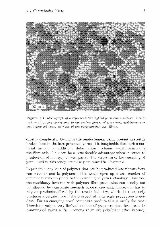
1.1 Micrograph of a representative hybrid yarn cross-section.
5
1.2 Schematic illustration of the stamp forming process ....10
2.1 Textile preforms 17
2.2 Viscosity vs. temperature 23
2.3 Permeability and vs. fibre volume fraction 27
2.4 Cross-sectional area and laminate thickness relationships .32
2.5 Schematic yarn cross-section during consolidation 36
3.1 Specific heat of different laminate components and PEEK 47
3.2 Thermal conductivity of PA-6 and PA-12 vs. temperature. 50
4.1 Resistance heating set-up 71
4.2 Conduction heating 72
4.3 Validity of the analytical solution 73
4.4 IR/convection heating vs. time and distance from clamp .74
4.5 Infra-red and convection heating 75
4.6 Electrical resistance heating 76
5.1 Micrograph of standard grade commingled yarn 86
Xll
5.2 Unconsolidated yarn cross section: PA 12 (A) 87
5.3 Unconsolidated yarn cross section: PA 12 (B) 88
5.4 Unconsolidated yarn cross section: PBT 89
5.5 Cumulated fibre length distributions 90
5.6 Yarn winding frame 91
5.7 Flexural strength along the fibre direction 93
5.8 Tensile strength transverse to the fibre direction 95
5.9 Laminate temperature during consolidation 96
5.10 Schematic illustration of crack formation 98
5.11 Micrographs of consolidated laminate cross-sections. . .
103
5.12 Void characterisation 107
6.1 Experimental set up 114
6.2 Discretisation in time and space 116
6.3 Temperature of crystallisation onset vs. cooling rate....
121
6.4 Isothermal crystallisation kinetics 122
6.5 Flow chart of the heat transfer model 126
6.6 Temperature profile at low press plate temperature ....127
6.7 Temperature profile at high press plate temperature . . .128
6.8 Effect of thickness of the insulating tool 130
6.9 Void content and viscosity as a function of cooling time.131
6.10 Void content evolution for different yarn architectures. .
132
6.11 Void content evolution of PBT yarn type 134
6.12 Void content of PBT yarn type processed in steel moulds 135
7.1 Schematic illustration of the yarn winding plate 141
7.2 Schematic illustration of the consolidation of sample ends. 142
7.3 Photograph of a partially consolidated sample 143
7.4 Tensile test machine 145
7.5 Water cooled chuck head 146
7.6 Herschel-Bulkley model 146
7.7 Square and hexagonal fibre packing geometry 148
7.8 Flow curve of the micro-mechanical model 150
7.9 Definition of the circular unit cell 153
7.10 Fibre length distribution 160
7.11 Viscosity contribution 162
7.12 Flow curves of the CF50 yarn 163
7.13 Flow curves of the CF56 yarn 164
7.14 Flow curves of the CFs yarn 165
7.15 Flow curves at scaled fibre length distribution 166
7.16 Flow curves at different degrees of fibre wetting 169
7.17 Flow curves at different fibre volume fractions 170
7.18 Fibre volume fraction dependent factors 171

xiv

List of Tables
1.1 Properties of high tenacity carbon fibres 4
1.2 Fabrication techniques for thermoplastic composites ...8
2.1 Arrhenius parameters and molecular weight 22
2.2 Calculation of cross-sectional areas 33
4.1 Heating parameters 77
5.1 Designation, yarn and processing parameters 85
5.2 Mechanical properties 94
5.3 Parameters of the Cooling Curve Fit 97
5.4 Yarn and viscosity parameters 100
5.5 Measured and Calculated Void Content 102
6.1 Materia] Parameters 124
6.2 Statistical yarn characteristics 133
7.1 Yarn Parameters 144
7.2 Model parameters 165

xvi

List of Symbols
In general, subscript indices i and superscript indices k indicate spatialand temporal coordinates, respectively. The spatial coordinate alwayscoincides with the out-of-plane direction of a flat laminate. The sub¬
script index j refers to the considered fibre bundle size class. Indices f
and m—regardless whether subscript or superscript—generally address
quantities which are in relation to reinforcement fibres and matrix, re¬
spectively. Finally, symbols carrying a ~ describe properties belongingto a given moulding tool material. Symbols set between { ) represent
average values.
Latin Symbols
a Thermal diffusivity;
Fitting parameter
a0 Major half-axis length of an ellipsoidal fibre bundle
at Coefficient
am Surface fraction of polymer fibres
«¥ Specific surface area
A Fitting parameter;
Total area of interaction
A Coefficient matrix
Ab Area of reinforcing fibre bundle
-4ev External void area

xviii
Af Area of reinforcing fibres in a yarn
A-lv Internal void area
.4m Area covered by matrix in a yarn or laminate cross-section
Ai Total area of an entirely consolidated yarn or unit cell area
Acu Circular unit cell area
Au Unit cell area
A Fibre to non-fibre volume ratio
b Fibre bundle width;
Fitting parameter
6q Minor half-axis length of an ellipsoidal fibre bundle
b, Coefficient
B Fitting parameter
Bi Biot number
C; Coefficient
cp Specific heat of the laminate
C Integration constant
Cm Initial infra-red heating contribution
Cjn Infra-red heating contribution at end of heating
C Geometric parameter related to the degree of commingling
d Differential
d Laminate thickness;
Fitting parameter
d Partial differential
d Moulding tool thickness
Ea Activation energy for viscous flow
Ep Elastic constant due to frictional effects
Enl Tensile modulus at thermoforniing temperature
,/ Factor related to the fibre volume fraction
F Force
F Maximum force
Ff Frictional force
F\ Normal force
F\o Normal force in case of full wetting
Fo Fourier number
g Factor related to the fibie volume fi action
G Geometric constant according to Gebart
h Instantaneous laminate thickness
h* Dimensionless cylinder height
ho Height of a fully consolidated vain
ftoo Minimum possible laminate thickness
h\y Laminate thickness if fibie bundles are cluster
hç Fully consolidated laminate thickness
/i, Laminate thickness at matrix coalescence
77t Latent heat of polymer crystallisation
I Electrical current density
k Avi ami coefficient
k' Gutowski constant
A'p - Gencial peimeabilit) ;
- Peimeabilitv accoiding to Gebart's model
KpK Peimeabilitv according to Carman-Kozeny
KpU Permeability according to Gutowski
L Correction factor
£ Reinforcement fibre length
I* Relative reinforcement fibre length
£m Polymer fibie length
£ma^ Maximum fibre length
fmin Minimum fibre length
A( Length diffeience between fibre length classes
L Penetration distance in flow direction;
Arbitrary scaling length

Lq Undamped sample length
My, Weight-average molecular weight of polymers
n - Exponent;- Total number of size classes;- Relative number of fibres at a given length class
-V (tm) Number of fibres of length class lm
ATa Total number of fibre bundles in a laminate cross section
A'l Number of fibres in a fibre bundle
at optimal commingling
(ATf) Number of reinforcement fibres
to be wetted by one polymer fibre
A7f Total number of reinforcing fibres in a
laminate or yarn cross-section
Nj Number of fibre bundles in a yarn cross-section
containing A7J fibres
Arj Number of fibres contained in the jth fibre bundle size class
-^niax Maximum number of fibres contained in the largest bundle
ATp Number of laminate plies
p Number of fibre length class
P - Instantaneous local pressure;
- Maximum number of fibre length classes
Pq Atmospheric pressure
Pa Applied pressure
Pc Capillary pressure
Pf Pressure carried by the dry fibre bed
Pm Pressured carried by the liquid matrix
Pv Void pressure
V Electrical power input
q Number of relative interaction length class
</o Net heat flow transmitted into the preform
Q Maximum number of relative interaction length classes
XXI
Q Heat generation term due to crystallisation
Q Spatial heat generation vector
r Void radius
r* Dimensionless cylinder radius
r° Equivalent circular fibre bundle radius before compaction;
Initial void radius
rt Critical void radius
r(u Radius of the circular unit cell
req Equivalent circle radius
n Reinforcement fibre radius
rh Hydraulic radius
rm Polvmer fibre radius
R Universal gas constant
R Distance from fibre surface, where the velocityof the flow medium is null
R2 Pearson correlation coefficient
Re Reynolds number
s'2 Variance of a statistical distribution
5 Fibre spacing
5b Fibre bundle spacing
5„ Eshelby tensor
t Time
t Total heating time
tL Consolidation time elapsed until crystallisation onset;
Absolute crystallisation time
ta Time elapsed until the maximum stress is reached
T Temperature
T Spatial temperature vector
T - Temperature at tool surface;
Tempeiature of heating plates
xxii
T Laminate temperature at end of heating
(T) Average temperature
Tq Initial temperature
ïi, Preform surface temperature
Tc Polymer crystallisation onset temperature
Pcotw Temperature of the convective medium
Tm Polymer melting temperature
7Y[ Midplane temperature
Tp Press plate temperature
Traci Surface Temperature of quartz glass radiators
u Elongational velocity
u^_ Transverse velocity of fibre moving through matrix
Uf Radial fibre velocity due to bundle compaction
uiiq Superficial velocity of the fluid in Darcy's law
um Matrix velocity
un nth solution of the transcendent equation u tan« = Bi
U Electrical potential difference (Voltage)
u° Specific volume of amorphous polymer
t'J? Specific volume of crystalline polymer
w Wetting parameter
we Yarn weight per unit length
Wf Fibre mass fraction
wm Matrix mass fraction
VV Laminate width
x - Coordinate transverse to the fibre direction;
- Flow front position
Xç Volume fraction of crystalline polymer
xxm
Greek Symbols
a Heat transition coefficient
aa Volume expansion coefficient of amorphous polymer
qc Volume expansion coefficient of crystalline polymer
at Length expansion coeffiecient
av Volume exi)ansion coefficient
3 Fitting parameter;
Exponent
'Yn Filler's constant
1i Imaginary shear angle
^)k Surface tension of the wetting liquid towards vacuo
ö Relative interaction length
AS Difference between subsequent
relative interaction length classes
e Strain
è Strain rate
ê Strain at maximum stress
£e Elastic strain rate component
s\ Elastic strain in stage (I) of the flow curve
c" Elastic strain component in stage (11) of the flow curve
ép Plastic strain rate component
(, Combined probability function
j] Viscosity
i]m Viscosity of the polymer melt
i/mo Viscosity of the polymer melt at infinite temperature
9 Twist factor
0 Fibre orientation angle
K{ Elastic constant of a compressed dry fibre bed
À = An Transverse thermal conductivity of the laminate
xxiv
A Thermal conductivity of the moulding tool material
Aq Transveise thermal conductivity of
impregnated laminate portions
AAir Thermal conductivity of air
Afa Transveise thermal conductivity of fibre agglomeiations
Ajj Anisotropic thermal conductivity of void free laminate
Xln Anisotropic thermal conductivity of carbon fibres
Am Thermal conductivity of polymer matrix
ß* Predictand of a logarithmic normal distribution
p\lT Friction coefficient in case of aii lubrication
fiF Total friction coefficient
fim Friction coefficient for lubricated friction
i/f General fibie volume fi action,
i.e., in the fully consolidated laminate
Ff Normalised fibre volume fraction
i\ Void content
Uy Initial void content
p- Instantaneous laminate density:
- Measured laminate density
p Density of moulding tool material
PAir Density of aii
pi Fibre density
pm Matrix density
Pi Theoretical laminate densitv
a Stress
a Maximum stiess
(Tq Maximum stress of entirely wetted fibre material
<tt Elastic stress in stage (I) of the flow curve
a11 Elastic stress component in stage (II) of the flow curve
<7f Effective stress tensor component in radial direction
XXV
<7f Stress due to friction between interacting fibres
er" Plastic stress component
<Ji Stress in total statistical fibre material
<y Tortuosity
h'o Initial fibre volume fraction
v Theoretic maximum fibre volume fraction
Vf Fibre volume fraction in dry compressed fibre agglomerations
fnia-ï Experimental maximum fibre volume fraction
i v Porosity
ç> Probability function
Kp Contact angle
X Amorphous to crystalline polymer conversion
v Probability function

xxvi

Chapter 1
Introduction
Composite Materials have a long historical tradition in human technol¬
ogy. Already the ancient Egyptians understood that a suitable combina¬
tion of two different materials may result in a new material with better
performance than the sum of properties of each component [1]. The
improvement of mechanical properties is thereby not always the drivingforce for the design or use of a composite material. Even economical
considerations can provide such a driver for the use of composites; e.g.
in case of furniture design where a cheap core material is covered by a
high quality surface.
However, for engineering applications new composite materials can onlybe successfully invented if they are able to fulfil an entire catalogue of
requirements. Depending on the type of application, they might be (notin order of priority):
« mechanical properties,
« resistance against environmental impacts,
« wear resistance.
« damage tolerance,
« functionality,
« low price,

2 Introduction
An uncountable number of different composite material systems are
known today and these only lepresent the beginning of a new gener¬
ation of materials. They all have one thing in common: Each compositematerial exhibits properties that could not be achieved with one single
homogeneous material.
Despite the obvious advantages of composite materials, production vol¬
umes of high performance composites based on reinforced polymers did
not follow vet a steep curve as predicted shortly after the emergence of
such materials. In the case of load bearing structural parts, the advan¬
tage of theii excellent strength-to-weight performance is often defeated
by the high material costs and labour intensive production routes for
composite parts.
The use of thermoplastics as matrix materials may offer a promising ap¬
proach to overcome some of the limitations of theimosetting polymersas far as large volume production is concerned. Curing of thermosettingresins requires a chemical leaction whereas thermoplastics simply un¬
dergo a phase transformation from the molten to the solid state. Since
the thermosetting resin viscosity progiessivelv increases with elapsingreaction time, first the termination reaction and finally the propagationreaction itself become diffusion controlled [2]. Diffusion velocity, how¬
ever, is strongly dependent on Temperatuie but is in general relativelyslow compared to polymer solidification from the melt, which mainly
depends on the cooling rate. As a matter of fact, process cycle times of
thermoplastic products are on the range of a few seconds whereas curingof theimosetting resins is usually on the ordei of several ten minutes and
often even hours.
Although (quasi-)continuously fibre reinforced thermoplastics can be
produced fastei than reinfoiced theimosetting resins, process cvcle times
of unfilled or short fibre reinfoiced polymers remain unmatched. This
is mainly due to the high viscosity of thermoplastic resins, which makes
impregnation of high volume fraction fibre beds difficult. Despite the rel¬
atively fast processing cycle times for high perfoimance fibre reinforced
thermoplastics as compared with their thermosetting competitors, in
1990, only 3 % of the total market for polymer matrix structural com¬
posites was covered by composites with thermoplastic matrix [3]. This
also has to be attributed to the inherent difficulties of fibre impregna¬tion. Several solutions were proposed to "pie impregnate" the fibres to
overcome the problem of fibre wetting. The resulting prepregs are rela¬
tively stiff and boardy, limiting their handling and drapeability during
manufacturing, and, thus, severely affecting the achievable part geom-
1.1 Commingled Yarns 3
etry complexity. Consequently, prepregging techniques are particularlysuited for the manufacture of relatively small series of large and flat
structures. As the interest for the fabrication of larger series of smaller
and more complex shape composite parts increases, there is a growingdemand for more drapeable and easy-to-handlc precursors. Novel pro¬
cessing techniques need to be explored to manufacture complex geometry
composite parts made of fibre reinforced thermoplastics.
Finding an ideal compromise between production costs, part geometry
complexity, and high mechanical properties is these days' challenge in
composite materials development. Particularly the problem of lowering
production costs by simultaneously maintaining material performance is
difficult to solve. Injection moulding of long-fibre reinforced polymermasses allows for producing complex shaped, three-dimensional parts,
but the fibre volume fraction is limited to values at which their reinforc¬
ing effect is inefficient. Furthermore, the fibres are generally not aligned.On the other hand, fully consolidated tapes with unidirectional contin¬
uous fibre reinforcement are available at high fibre volume fractions and
offer extremely efficient use of the reinforcing fibres in terms of transmit¬
ting mechanical loads, but such tapes are difficult to set into shell like
structures with heavy two-dimensional curvature. As a compromise be¬
tween these two extremes a number of other intermediate products have
been developed—some of these will be discussed in Section 2.2. aimingat cost efficient part production by simultaneously achieving satisfactorymaterial performance.
1.1 Commingled Yarns
Due to the high melt viscosities of thermoplastic polymers, the matrix
has to be combined with the fibres already at the preform stage in such
a way. that the polymer does not have to flow long distances to achieve
fibre wetting during consolidation. Probably the greatest potential for
further shortening of impregnation time lay in the advancement of com¬
bination techniques.
Commingling of thermoplastic fibres and reinforcing fibres can deliver
the requested intimate blending at the preform stage and such interme¬
diate products have been commercialised quite some time ago [4]. One of
the outstanding advantages of commingled yarns lies in their potential of
intimate blending of reinforcement and matrix fibres by simultaneously
4 Introduction
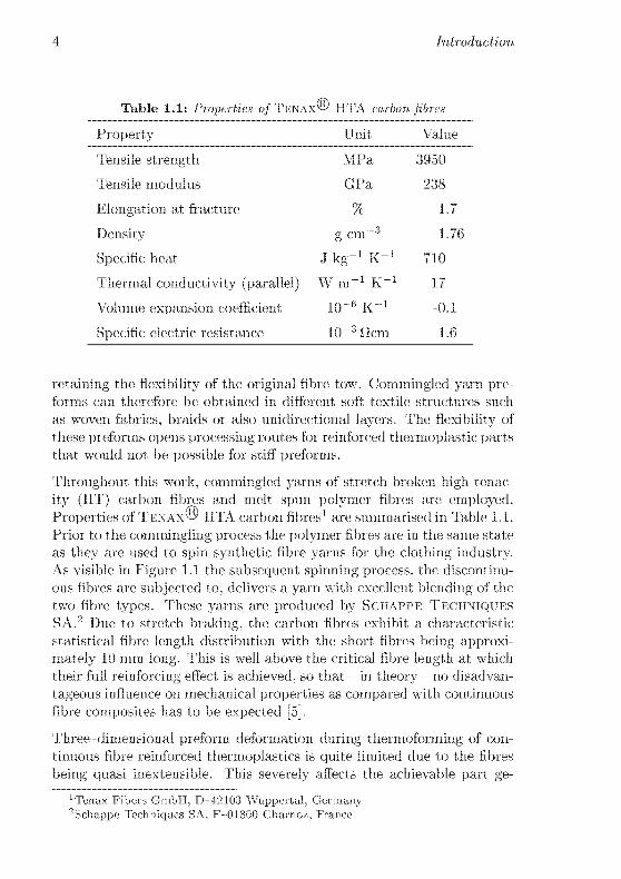
Table 1.1: Properties o/Tknax^ HTA carbon fibres
Property Unit Value
Tensile strength MPa 3950
Tensile modulus GPa 238
Elongation at fracture % 1.7
Density g cm"3 1.76
Specific heat J kg1 K1 710
Thermal conductivity (parallel) W m"1 K""1 17
Volume expansion coefficient 10-G K-i -0.1
Specific electric resistance lQ~~3Ocm 1.6
retaining the flexibility of the original fibre tow. Commingled yarn pre¬
forms can therefore be obtained in different soft textile structures such
as woven fabrics, braids or also unidirectional layers. The flexibility of
these preforms opens processing routes for reinforced thermoplastic parts
that would not be possible for stiff preforms.
Throughout this work, commingled yarns of stretch broken high tenac¬
ity (HT) carbon fibres and melt spun polymer fibres are employed.
Properties of Tenax UTA carbon fibres1 are summarised in Table 1.1.
Prior to the commingling process the polymer fibres are in the same state
as they arc used to spin synthetic fibre yarns for the clothing industry.As visible in Figure 1.1 the subsequent spinning process, the discontinu¬
ous fibres are subjected to. delivers a yarn with excellent blending of the
two fibre types. These yarns are produced by Schappe Techniques
SA.2 Due to stretch braking, the carbon fibres exhibit a characteristic
statistical fibre length distribution with the short fibres being approxi¬
mately 10 mm long. This is well above the critical fibre length at which
their full reinforcing effect is achieved, so that in theory no disadvan¬
tageous influence on mechanical properties as compared with continuous
fibre composites has to be expected [5].
Three dimensional preform deformation during thermoforming of con¬
tinuous fibre reinforced thermoplastics is quite limited due to the fibres
being quasi inextensible. This severely affects the achievable part ge-
'Tenax Fibers GmbH, D -12103 Wuppertal. Germany
2Schappe Techniques SA, F 01800 Charnoz, France
1.1 Commingled Yarns 5
Figure 1.1: Micrograph of a representative hybrid yarn cross-section Brightand small circles correspond to the carbon fibres, whereas dark and larger cir¬
cles lepresent cross-sections of the poly(laurolactam) fibres
ometry complexity. Owing to the reinforcement being present in stretch
broken form in the here presented varns. it is imaginable that such a ma¬
terial can offer an additional deformation mechanism—extension alongthe fibre axis. This can be a considerable advantage when it comes to
pioductioii of multiply curved parts. The structure of the commingled
yarns used in this study aie closely examined in Chapter 5.
In principle, any kind of polymer that can be produced into fibrous form
can serve as matrix polymer. This would open up a vast number of
different matrix polymers to the commingled yarn technology. However,the machinery involved with polymer fibre pioductioii can usually not
be affoided by composite reseaich laboratories and, hence, one has to
rely on products offered by the textile industry, which, in turn, out¬
produces a certain fibre if the prospect of large scale production is evi¬
dent. For an emerging novel composite pioduct this is rarely the case.
Therefore, only a very limited number of polymers have been used in
commingled yarns so far. Among them are poly (ether ether ketone),
6 Introduction
poly(propylene), poly (ethylene terephthalate), poly(caprolactam), and
poly(laurolactam). These are readily available on the textile market and
they have been used for production of thermoplastic matrix compos¬
ites for quite some time. Especially poly(laurolactam) is widely used in
combination with carbon fibre reinforcement. The relatively high price
of poly(laurolactam), however, depicts a considerable drawback of this
engineering plastic. In the present study commingled yarns of carbon
and poly(laurolactam) fibres arc used at a variety of yarn architectures
featuring two different carbon fibre length distributions and carbon fibre
volume fractions. Additionally, a yarn of carbon fibres intermingled with
poly(butylene terephthalate) fibres is subjected to direct stamp formingand the resulting laminate properties are compared with those of the car¬
bon fibre poly(laurolactam) laminates. Poly(butylene terephthalate) is
not as costly as poly(laurolactam) and. moreover, offers better mechan¬
ical properties at elevated temperatures. This is an important criterion
for the automotive industry and it often decides whether or not a givenmaterial can be employed to produce a certain part.
1.2 Production Techniques for Aligned Fi¬
bre Reinforced Thermoplastic Parts
To achieve the goal of relatively low cost structural fibre reinforced ther¬
moplastic parts not only suitable intermediate products have to be in¬
vented but also corresponding processing technologies need to be devel¬
oped. According to Tadmor and Gogos [6] any polymer processing route
consists of an invariant chain of variable process steps that are namely:
1. polymer liquiditying,
2. shaping (usually by applying pressure),
3. setting (e.g. curing or solidifying), and
4. finishing.
Basically, there are two groups of thermoforming processes following this
concept:
1. Preform heating (liquidifying), shaping, fibre impregnation, and
cooling (setting) takes place in a closed moulding tool capable of
1.2 Production Techniques
heating and cooling. Not consolidated, soft textile preforms may
be used.
2. The preform is heated outside of the moulding device (liquidify¬ing) and transferred to the moulding tool, where the reinforced
polymer is pressurised to be shaped, and solidified (set) almost
simultaneously. The tool's temperature is maintained constant be¬
low the thermoplastic's melting temperature to ascertain shape
setting before demoulding. Cooling is therefore very fast and thus
the process usually requires preforms which have been entirely con¬
solidated prior to shaping.
The process cycle time of the former is on the order of 10 minutes whereas
the tool occupancy time of the latter is on the scale of several 10 seconds.
The advantage of short process cycle times in the latter case is, however,at least partially defeated by the necessity of employing consolidated
sheet-like intermediate products.
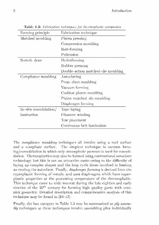
More than twenty different fabrication techniques have been identified
for thermoplastic composites [7]. The principal techniques as they have
been summarised by Cattanach and Cogswell [8] are given in Table 1.2.
In the matched moulding technique the material is melted and then
shaped between two matched dies. The dies must be carefully machined
and aligned to provide equal consolidation pressure over the whole sur¬
face area of the moulded part. Roll-forming and pultrusion offer the
possibility of continuous production of channels, beams and similar ar¬
ticles. Further information on the roll-forming technique may be found
in [8].
Stretch draw moulding is a term that originates in the moulding tech¬
nology for metallic sheets. Here and henceforth, this technique will be
referred to as stamp forming when it is used in connection with the rapid
moulding of unconsolidated commingled yarn preforms as they are dealt
with throughout this work. The preform is thereby heated to process
temperature and then rapidly transferred to the moulding device, which
can consist of male and female matched dies, a male rubber and female
metal mould or vice versa. An overview of rubber forming techniques as
they are referred to if one mould half consists of an elastic rubber like
material can be found in [9]. In case of hydroforming only one solid
tool half is used and the consolidation pressure is transmitted by an
incompressible fluid (usually this will be a synthetic oil).
8 Introduction
Table 1.2: Fabrication techniques for thermoplastic composites
Forming principle Fabrication technique
Matched moulding Platen pressing
Compression moulding
Roll forming
Pultrusion
Stretch-draw Hydroforming
Rubber pressing
Double-action matched-die moulding
Compliance moulding Autoclaving
Press clave moulding
Vacuum forming
Cushion platen moulding
Piston matched-die moulding
Diaphragm forming
In situ consolidation/ Tape laying
lamination Filament winding
Tow placement
Continuous belt lamination
The compliance moulding techniques all involve using a tool surface
and a compliant surface. The simplest technique is vacuum form¬
ing/consolidation in which only atmospheric pressure is used for consoli¬
dation. Thermoplastics may also be formed using conventional autoclave
technology, but this is not an attractive route owing to the difficulty of
laying up complex shapes and the long cycle times involved in heatingan cooling the autoclave. Finally, diaphragm, forming is derived from the
superplastic forming of metals, and uses diaphragms which have super-
plastic properties at the processing temperature of the thermoplastic.This technique came to wide interest during the late eighties and earlynineties of the 20 century for forming high quality parts with com¬
plex geometry. Detailed description and comprehensive analysis of this
technique may be found in [10-13].
Finally, the last category in Table 1.2 may be summarised as ply assem¬
bly techniques as these techniques involve assembling plies individually
1.3 Stamp Forming of Unconsolidated Commingled Yarn Preforms 9
to make an intermediate or final product. The goal with these techniquesis to melt the prepreg tape or tow and consolidate it locally in a single
operation. The heating energy is thereby focused on the place of instan¬
taneous consolidation. Several suitable heat sources have been identified,
including laser, infra-red, flame, hot gas and heated shoe [14]. The tape
laying technique has been comprehensively analysed in terms of thermal
phenomena during the process of in-situ consolidation by Toso [15].
1.3 Stamp Forming of Unconsolidated Com¬
mingled Yarn Preforms
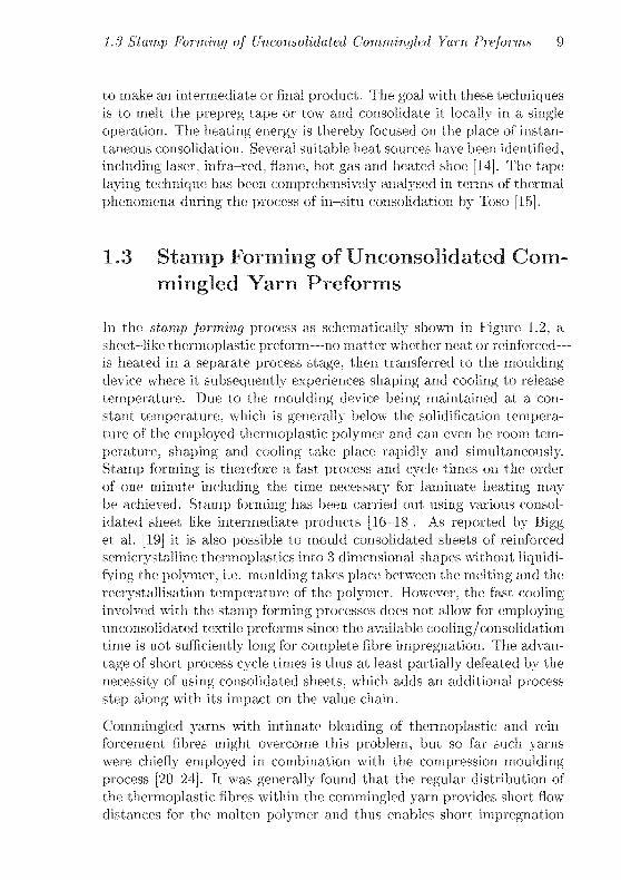
In the stamp forming process as schematically shown in Figure 1.2, a
sheet like thermoplastic preform no matter whether neat or reinforced
is heated in a separate process stage, then transferred to the mouldingdevice where it subsequently experiences shaping and cooling to release
temperature. Due to the moulding device being maintained at a con¬
stant temperature, which is generally below the solidification tempera¬
ture of the employed thermoplastic polymer and can even be room tem¬
perature, shaping and cooling take place rapidly and simultaneously.
Stamp forming is therefore a fast process and cycle times on the order
of one minute including the time necessary for laminate heating may
be achieved. Stamp forming has been carried out using various consol¬
idated sheet like intermediate products [16 18]. As reported by Bigget al. [19] it is also possible to mould consolidated sheets of reinforced
scmicrystallinc thermoplastics into 3 dimensional shapes without liquidi-
fying the polymer, i.e. moulding takes place between the melting and the
recrystallisation temperature of the polymer. However, the fast coolinginvolved with the stamp forming processes docs not allow for employingunconsolidated textile preforms since the available cooling/consolidationtime is not sufficiently long for complete fibre impregnation. The advan¬
tage of short process cycle times is thus at least partially defeated by the
necessity of using consolidated sheets, which adds an additional process
step along with its impact on the value chain.
Commingled yarns with intimate blending of thermoplastic and rein¬
forcement fibres might overcome this problem, but so far such yarns
were chiefly employed in combination with the compression moulding
process [20 24]. It was generally found that the regular distribution of
the thermoplastic fibres within the commingled yarn provides short flow
distances for the molten polymer and thus enables short impregnation

10 Introduction
^Denioulcling
Figure 1.2: Schematic illustration of the stamp forming process. The temper¬
atures k. Tm, T, and'F indicate the laminate temperature before transfer, the
polymer melting temperature, tht moulding tool ternperxiture. and the polymer
crystallisation température, respectively.
times. If commingled yarns arc, however, subjected to the stamp forming
process, the accessible consolidation time was observed to be too short
to obtain laminates with satisfactory residual void content [25], giventhe blending quality of the yarn the authors worked with. Wakeman ct
al. performed an extensive parameter study on stamp forming which
they refer to as non isothermal compression moulding of Twintex®
glass fibre poly(propylene) commingled yarn [26]. At optimised process¬
ing conditions they obtained laminates with approximately 1 % void
content.

1.4 Objective of the Thesis 11
1.4 Objective of the Thesis
The present Work focuses on the stamp forming of a novel commingled
yarn intermediate product. Layers of commingled yarns in fabric form or
unidirectional arrangement undergo the stamp forming process without
having experienced consolidation prior to moulding.
As stated above, the degree of intermingling of reinforcement fibres and
polymer in the preform state is generally not sufficient to allow for direct
stamp forming. This is, however, only a qualitative remark. Within this
work it is therefore aimed at providing both preform and processing char¬
acteristics under which the stamp forming process can deliver laminates
of satisfactory quality. Based on experimental results and theoretical
considerations, limits and potentials of this technique are implied.
In Chapter 2 post-impregnated product forms and their consolidation
are reviewed on a theoretical level. Both the heating and the mould¬
ing/consolidation/cooling steps represent, in principle, heat transfer
problems, where in case of the former, heat is transferred to the preformand in case of the latter the amount of heat absorbed by the preform dur¬
ing heating is transferred to the moulding device. For thermal calcula¬
tions a number of physical material parameters of the preform/laminateand of the mould are required. How these parameters can be deter¬
mined as functions of temperature and preform composition is shown in
Chapter 3 based on experimental work and/or literature review. Heat
transfer during heating and cooling are studied empirically and in the¬
ory in Chapters 4 and 6, whereas the influence of processing parame¬
ters on laminate quality is investigated mainly on an empirical level in
Chapter 5. Finally, the axial deformation behaviour of commingled yarn
preforms under thcrmoforming conditions is dealt with empirically and
by means of simulations based on the rheological behaviour of alignedfibre filled viscous fluids in Chapter 7.
References
[1] U. Meier. Verbundkonstruktionen als Entwicklungstrend. Schweizer
Ingenieur und Architekt (37), 1994.
[2] M. R. Kama! and S. Sourour. Kinetics and thermal characterization
of thermoset cure. Polymer Engineering and Science, 13(1):59 64,
1973.

12 Introduction
[3] F. N. Cogswell. Thermoplastic Aromatic Polymer Composites.Butterworth Ileinemann. 1992.
[4] S. IL Olsen. Manufacturing with commingled yarn, fabrics and
powder prepreg thermoplastic composite materials. SAMPE Jour¬
nal, 26:31 36, 1990.
[5] I. Al. Robinson and J. M. Robinson. The influence of fibei aspect 1a-
tio on the deformation of discontinuous fiber-reinforced composites.Journal of Materials Science, 29(18) =4663-4677. 1994.
[6] Z. Tadmor and C. G. Gogos. Principles of Polymer Processing.
Wiley. 1979.
[7] J. A. Barnes and J. B. Cattanach. Advances in thermoplastic com¬
posite fabrication technology. In Proceedings of the Materials Engi¬
neering Conference, London, UK, 1985.
[8] J. B. Cattanach and F. N. Cogswell. Advances in thermoplastic
composite fabrication technology. In G. Pritchard. editor, Devel¬
opments in Reinforced Plastics, chapter 5. Elsevier Applied Science
Publishers. London, UK, 1985.
[9] L. M. J. Robroek. The Development of Rubber Forming as a Rapid
Thcrmoforming Technique for Continuous Fibre Reinforced Ther¬
moplastic Composites. PhD thesis, Technische Universiteit, Delft,
Netherlands. 1994.
[10] P. J. Mallon and C. AI. O'Bradaigh. Polymeric diaphragm formingof continuous fibre reinforced thermoplastics. In Proceedings of the
33rd SAMPE Symposium, pages 47-61, Anaheim, 1988.
[11] P. J. Mallon and C. Al. O'Bradaigh. Development of a pilotautoclave for polymeric diaphragm forming of continuous fibre-
reinforced theimoplasitcs. Composites. 19(l):37-47, 1988.
[12] P. J. Mallon and C. Al. O'Bradaigh. Polymeric diaphragm formingof complex cuivatuie thermoplastic composite parts. Composites,
20(1):48 56, 1989.
[13] S. Delaloye. Die Diaphragma Technik, em Anlagenkonzept zur
automatisierten Fertigung kontinuierlich faserverstärkter Thermo-
plastbauteile. PhD thesis, Swiss Federal Institute of Technology,Zurich, Switzerland. 1995. Diss. ETII No. 11151.

1.4 References 13
[14] M. W. Egerton and M. B. Gruber. Thermoplastic filament windingdemonstration of economics and properties via in situ consolida¬
tion. In Proceedings of the 33rd SAMPE Symposium, pages 35 46,
Anaheim. 1988.
[15] Y. P.-M. Toso. Effective Automated Tape Winding Process with On-
Line Bonding under Transient Thermal Conditions. PhD thesis,Swiss Federal Institute of Technology, Zurich, Switzerland, 2003.
Diss. ETH No. 14983.
[16] U. Breuer and M. Neitzel. High speed stamp forming of thermoplas¬tic composite sheets. Polymers & Polymer Composites, 4(2) = 117-
123, 1996.
[17] K. Friedrich and Al. Hon. On stamp forming of curved and flexi¬
ble geometry components from continuous glass fiber/polypropylenecomposites. Composites Part A, 29A:217 226. 1998.
[18] M. IIou. Stamp forming of fabric-reinforced thermoplastic compos¬
ites. Polymer Composites, 17(4):596 603, 1996.
[19] D. M. Bigg and J. R. Preston. Stamping of thermoplastic matrix
composites. Polymer Composites, 10(4) =261 268, 1989.
[20] L. Ye, K. Friedrich. J. Kastei, and Y.-W. Alai. Consolidation of
unidirectional cf/peek composites from commingled yarn prepreg.
Composites Science and Technology, 54(4):349 358, 1995.
[21] II. Ilamada, Z.-T. Maekawa, N. Ikegawa, and T. Alatsuo. Influence of
the impregnation property on mechanical properties of commingled
yarn composites. Polymer Composites, 14(4):308-313, 1993.
[22] B. Lauke, U. Bunzel, and K. Schneider. Effect of hybrid yarn struc¬
ture on the delamination behaviour of thermoplastic composites.
Composites Pari A, 29AT397-1409. 1998.
[23] P. McDonnell, K. P. McGarvey, L. Rochford, and C. Al. O'Bradaigh.
Processing and mechanical properties evaluation of a commingled
carbon-fibre/pa-12 composite. Composites Part A, 32:925-932,2001.
[24] J. Vendramini. C. Bas, G. Merle, P. Boissonnat, and N. D. Alberola.
Commingled poly(butylene terephthalate)/unidirectional glass fiber
composites: Influence of the process conditions on the microstruc¬
ture of poly(butylene terephthalate). Polymer Composites, 21:724
733, 2000.
14 Introduction
[25] X. Bernet, V. Vlichaud. P.-E. Bourban, and J.-A. E. Alânson. Com¬
mingled yarn composites for rapid processing of complex shapes.
Composites Part A, 32:1613 1626, 2001.
[26] Al. D. Wakeman. T. A. Cain, C. D. Rudd, R. Brooks, and A. C.
Long. Compression moulding of glass and polypropylene compositesfor optimised macro and micro mechanical properties 1 commin¬
gled glass and polypropylene. Composites Science and Technology,58:1879 1898, 1998.
Chapter 2
Consolidation of
Commingled Yarns
2.1 Introduction
Although thermoplastic matrices exhibit a number of favourable prop¬
erties and show considerable potential for reducing manufacturing costs,
extending product lifecycle and improving performance one major draw¬
back remains to be eliminated to open aligned long fibre reinforced ther¬
moplastic composites a wider field of applications: This is the high melt
viscosity of typically 200 5000 Pa-s as compared to 0.2 10 Pa-s usuallyobserved for conventional thermosetting polymers. High melt viscosities
are disadvantageous for fibre impregnation. The influence of the resin
viscosity on the impregnation rate can be demonstrated by Darcy's law,
describing laminar flow of fluids through homogeneous porous media [1].If only one dimensional flow is considered, Darcy's law7 appears as:
al K„0P.„,.
u]iq = vv— =*— 2.1)
at r] ox
where '«nq is the superficial velocity of the fluid, ?;v is the porosity of the
porous medium, L is the penetration distance in the x direction, t is the
time. Kp is the permeability of the porous medium, j] is the viscosityof the fluid, and P is the pressure acting along x to enable the fluid to
advance through the porous medium. Under the assumption of constant
permeability the time the fluid requires to entirely infiltrate the porous
16 Consolidation of Commingled Yarns
medium can be estimated as:
t=-2«,.(£-ft) '"»
where Pa designates the applied pressure to enhance flow and Pn is the
atmospheric pressure. According to Equation (2.2) a solution to over¬
come the problem associated with the high viscosity of polymer melts
is to minimise the flow distance for impregnation, L. This insight led
to the development of a number of different preform types, which are
discussed in the next section.
2.2 Post-Impregnated Product Forms
In Figure 2.1 the different principles of post-impregnation arc schemati¬
cally illustrated (in order of decreasing impregnation distance).[ Whereby
pre impregnated forms are ones in which the reinforcing fibres are com¬
pletely wetted and impregnated with the matrix; as opposed by the post
impregnated forms which achieve only a physical mixing of the matrix
and fibre and do not give full wetting of the reinforcement [2]. Since
commingled yarns belong to the latter category of intermediate productforms only post-impregnation techniques are considered here, i.e. the
polymer is not molten or dissolved to be blended with the reinforcingfibres:
1. Film stacking was one of the first techniques to be used and may
be applied to any thermoplastic that can be converted into a film.
Layers of fibre reinforcement, in the form of unidirectional tows or
woven fabrics, are thereby alternated with layers of thermoplasticfilms. Impregnation is achieved by applying heat and pressure.
Details about processing principles can be taken from [3]. It is
possible to produce components from combinations of fibres and
polymer which are not commercially available in prcpreg form.
Due to the poor quality of fibre/matrix blending (i.e. long impreg¬nation distance L) high pressures (on the order of 10 AlPa) and
long moulding times (usually longer than 30 min) are required to
1 The qualitative order after impregnation distance shown in Figure 2.1 is not rigidbut strongly depends on the actual quality of a given product form, e.g.. a powdercoated tow can offer smaller impregnation distance than a not well blended commin¬
gled yarn.

2.2 Post-Impregnated Product Forms 17
Film stacking
Figure 2.1: Schematic illustration of dry pre-irnpregnation techniques accord¬
ing to Leach [2].
achieve full consolidation [4, 5]. This procedure therefore only qual¬ifies for small number of parts to be produced. Polymer films can
only be very moderately deformed into two-dimensional curvature
shapes without wrinkling or buckling. If a single step production is
considered, the achievable geometry complexity of this method is
very limited. The problem can be circumvented by first producinga consolidated flat sheet and subsequently subjecting it to stamp
forming.
2. Cowoven fabrics consist of reinforcement fibre tows and polymerfibre tows in weft and warp direction or vice versa. The techniquehas the simplicity of being a textile operation and is therefore easy
to perform. The fabric is drapeable and hence product shapes fea-
JQO&SiT^XLMGLjO^rUc'u

18 Consolidation of Commingled Yarns
turing two dimensional curvature may be achieved. It can be prob¬lematic to obtain a certain polymer in fibre form as only a limited
number of different polymer fibres is readily available on the tex¬
tile market. The ease of impregnation depends on the weave styleand the size of the polymer and reinforcing fibre tows. Provided
a given polymer can be obtained in fibre form there is, theoreti¬
cally, no limit to the possible combinations of reinforcement fibres
and matrix polymer. Cowoven composites haven ben discussed bySilverman and Jones [6].
3. Powder coating is a combination of reinforcement fibre tows and
matrix polymer in powder form. There arc two product forms
using this impregnation technique, in Figure 2.1 referred to as
Powder coating and Powder coating with sheath, respectively:
(a) Powder coating: the spread fibre tow is immersed in a cham¬
ber where the polymer powder is fluidised with the aid of
turbulent air and polymer particles momentarily stick on the
tow due to static electric charges which originate in friction
of the fluidised particles [7-9]. Deposition by drawing the fi¬
bre tow through an aqueous powder dispersion has also been
reported [10]. Subsequently the powder coated tow has to be
heated above the polymer melting temperature to stabilise the
particles on the fibres. Melt fusing the particles to the fibres is
usually achieved by running the tow through an oven [7 10].An alternative has been demonstrated by Gantt et al. [11]where a direct current is applied to conductive fibres (e.g.carbon fibres), causing resistive heating and local melting of
the resin particles onto the fibres.
(b) Powder coating with sheath: exactly the same strategy is fol¬
lowed but the tow is additionally coated with a sheath of the
same polymer as the powder. This product form is widelyknown under the abbreviation FIT for Fibres Impregnatedwith Thermoplastic. Due to the enveloping polymer film it
is not necessary to melt fuse the polymer particles to sta¬
bilise them within the fibre tow. Consequently, a more flexi¬
ble preform is obtained. This inherent flexibility enables FIT
bundles to be readily run through a weaving operation to be
converted into a highly drapeable fabric suitable for the manu¬
facture of composite parts of complex geometry. High produc¬tion rates of textile fabrics can be attained owing to the pres¬
ence of the polymer sheath protecting the fibre tows against

2.2 Post-Impregnated Product Forms 19
abrasive wear. On the other hand, compared to molten pow¬
der towpregs, segregation of the powder from the fibres may
occur during normal handling, causing non uniform resin dis¬
tribution. Although the sheath is thin it is difficult to achieve
high fibre volume fractions as the sheath accounts for a con¬
siderable part of the whole polymer volume fraction. Either
the fibre fraction is thus relatively low or the impregnationdistance L is increased as a result of lower powder content.
A considerable advantage of powder coating is the availability of
almost any kind of polymer powder. Aloreover, most polymers
emerge from the polymerisation reaction in powder form, and thus
no additional processing is required for their use in powder coating,
resulting in a cost benefit of powder coated tows.
4. Commingling also known as Hybridisation involves an intimate
mixing of polymer and reinforcing fibres into a single tow. The
resultant hybrid tow (or yarn as it will be referred to henceforth)is normally woven into a fabric but can also be used in a uni¬
directional form [12]. This approach to reducing the impregna¬tion distance originated in a XASA contract for producing inti¬
mate blends of carbon with poly(butylene-tcrephthalatc) (PBT),poly (ether-ether-ketone) (PEEK), or a liquid crystal polymer [13].Intermingling of the reinforcing and thermoplastic fibres can be ob¬
tained by different techniques. One method involves jointly bulkingand intermingling the fibre by directional air jet [14]. In this case
the air pressure must be closely adapted to the reinforcing fibres so
as to achieve a uniform fibre distribution and at the same time min¬
imise damage to the fibres. Good blending results were achieved
with this technique of blends of carbon and PEEK fibres [12] as well
as glass and poly(propylene) (PP) fibres [15]. Another techniquewas developed by the Vetrotex company for the interdispcr-sion of continuous glass and thermoplastic (PP or poly(ethylenc-terephthalate) (PET)). These yarns arc commercially distributed
under the trade name Twintex®. The glass/polymer fibre ver¬
sions of Twintex© arc produced by conjointly manufacturingthe two fibre types and combine them at the end of the productionline [16, 17]. Schaffe Techniques developed a method for pro¬
ducing commingled yarns of various fibre and resin materials. In
this process both the reinforcing fibres and the thermoplastic fibres
are first stretch broken from continuous filaments to yield staplefibres. The subsequent spinning process gives a commingled yarn
20 Consolidation of Commingled Yarns
with a homogeneous blend of the two fibrous components. The dis¬
continuous nature of the fibres improves resistance to interlaminar
fracture [18] by simultaneously not affecting the tensile propertiesof consolidated laminates. Viscoelastic phenomena such as creep
of the composite in fibre direction might, however, result from the
discontinuity of the reinforcement fibres.
As with powder coating and coweaving, final impregnation is
achieved during the processing/fabrication stage. The quality of
the composite will depend upon the size and distribution of the
polymer fibres. The main drawbacks of this product form are the
limited availability of polymer fibres and the added preform costs
due to the commingling process.
2.3 Consolidation of Thermoplastic Com¬
posites
Very often it is not distinguished between the terms consolidation and
impregnation. In fact, impregnation refers to one stage of the whole
consolidation process. Consolidation consists of three main mechanisms,
namely:
1. intimate contact of the material components, usually achieved by
applying pressure,
2. autohesion of the polymer melt flow fronts, and
3. fibre bundle impregnation.
Work by Phillips ct al. [19] on consolidation of carbon fibre/poly (etherimidc) prepregs, however, support the assumption that intimate contact
and autohesion consume only a small portion of the total consolidation
time. This portion was quantified to be on the order of 1 %. The terms
consolidation and impregnation can, therefore, be seen as interchange¬able expressions. It was shown above that the key to fast impregnationis to provide short impregnation distance for the viscous polymer melt.
In case of the film stacking technique the time required to achieve full
fibre impregnation and thus an entirely consolidated laminate can eas¬
ily be estimated by using Equation (2.2), if the formation of entrappedvoids is neglected. In case of the other post impregnated product forms

2.3 Consolidation of Thermoplastic Composites 21
as presented above the situation is not as simple and a number of geo¬
metrical and/or statistical considerations have to be made to depict the
impregnation behaviour of such materials under the influence of pressure
and raised temperature. Several researchers were engaged in the devel¬
opment of impregnation models for powder coated intermediate productforms [20-23]. Consolidation of commingled yarns has been reviewed bySvensson and Shishoo [24],
Regardless of the employed post impregnated product form, there are
basically two parameters other than the impregnation distance to af¬
fect the total impregnation time necessary to achieve full consolidation,
namely they are the resin viscosity and the permeability of the fibre bed.
2.3.1 Resin Viscosity
The viscosity of thermoplastic polymers melts mainly depends on its
weight average molecular weight Mw. Viscosity differences among var¬
ious types of polymers arise due to the strength and frequency of sec¬
ondary bonds between adjacent polymer chains. From a technical pointof view the viscosity can be lowered by adding plasticisers. However,
when present in small amounts, plasticisers generally act as antiplas-
ticisers, i.e., they increase the hardness and decrease the elongation of
polymers. Inefficient plasticisers require relatively large amounts of these
additives to overcome the initial antiplasticisation. Good plasticiserssuch as di-2-ethylhexyl phthalate (DOP) change from antiplasticisers to
plasticisers when approximately 10 % of the plasticiser is added [25].But, generally spoken, it can be stated that the effect of plasticisersis not as significant as to change the polymer viscosity sufficiently to
overcome the problem of fibre impregnation.
The viscosity r/m of most of the technically important thermoplastic poly¬mers obeys an exponential function of the temperature, well known as
the Arrhenius relationship:
Vm(T) = r/mU exp f -^ J (2.3)
where nmo is the viscosity at infinite temperature.2 E& is the activation
energy for viscous flow. R is the universal gas constant and T is the ab¬
solute temperature. It has to be emphasised that the polymer viscosity
2assuming that the polymer would not decompose or in some other way changeits physical state

22 Consolidation of Commingled Yarns
is generally not Newtonian, i.e., it also depends on deformation veloc¬
ity. It is therefore also necessary to measure the viscosity a different
shear rates. Usually the plot of viscosity versus shear rate at a constant
temperature will exhibit only small or at least approximately linear de¬
pendence of viscosity on shear rate, which allows for extrapolating the
curve to obtain the polymer viscosity at zero shear rate.
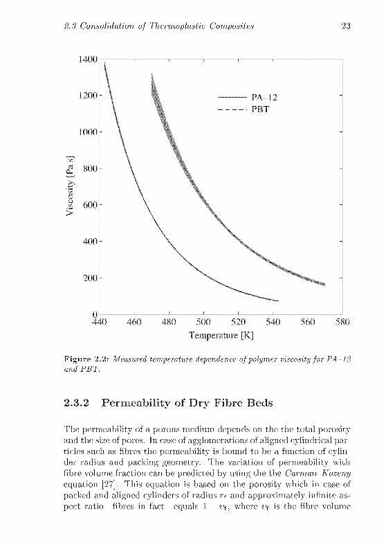
Oscillatory viscosity measurements of circular polymer samples of 13 mm
diameter and 2 mm thickness were performed on a Paar-Piiysica UDS
200 cone/plate viscosimeter. The shear amplitude and the oscillation
frequency were 10 % and 5 Hz, respectively. The experimental results
as shown in Figure 2.2 represent quasi continuous temperature scans at
a cooling rate of 1 °Cmiii_1 and oscilation frequency of 5 Hz at 10 %
strain amplitude. For each polymer 12 scans were performed and the
scatter band depicts the 99 % level of confidence as obtained by analysisof approximately 900 data points per polymer. In case of PA 12 the
scatter band is only barely visible due to very good agreement between
different runs.
PA-12 melts behave as Newtonian fluids in a wide range of shear rates
[26]. It was further assumed here that also PBT melts can be treated
as Newtonian fluids within the range of shear rates to be expected in a
thcrmoforming process. The temperature dependence of polymer melt
viscosity of both polymers as shown in Figure 2.2 is therefore assumed
to be valid for a range of shear rates up to moderately high values, also
covering deformation velocities at thcrmoforming conditions. Arrhenius
parameters to describe the temperature dependence of the viscosity for
both polymers as they were obtained from curve fitting as shown in
Figure 2.2 are given in Table 2.1.
Table 2.1: Arrhenius parameters and weight average molecular weight
Parameter Unit PA-12 PBT
Pa s 1.590-104 1.027-10"2
K 7.073-103 5.509-1Q3
g mol1 2.6-104 4.0-lQ'1
~m0
EAR
2.3 Consolidation of Thermoplastic Composites 23
440 460 480 500 520 540 560 580
Temperature [KJ
Figure 2.2: Measured temperature dependence of polymer viscosity for PA-12
and PBT.
2.3.2 Permeability of Dry Fibre Beds
The permeability of a porous medium depends on the the total porosityand the size of pores. In case of agglomerations of aligned cylindrical par¬
ticles such as fibres the permeability is bound to be a function of cylin¬der radius and packing geometry. The variation of permeability with
fibre volume fraction can be predicted by using the the Carman Kozeny
equation [27]. This equation is based on the porosity which in case of
packed and aligned cylinders of radius rf and approximately infinite as¬
pect ratio fibres in fact equals 1 — Vf. where Vf is the fibre volume
ItUU
1200
1000
£ 800
.1?o
.1 600
400
200
24 Consolidation of Commingled Yarns
fraction of the dry fibre bed, av is the specific surface area i.e., the
ratio of particle surface area to their volume, r^ is the hydraulic radius,and ç is the tortuosity . Assuming cylindrical pores the Carman Kozeny
equation yields the permeability Kp:K is:
-CK_
rh (1 - V[)
The hydraulic radius can be determined as [28]:
rh =^ (2-5)av vt
For cylindrical particles the specific surface area calculates to av = ~-
with the cylinder or fibre radius rr, and hence the Garman-Kozeny equa¬
tion becomes:
KT =^^ (2.6)
The tortuosity ç, which is usually referred to as the Carman Kozenyor Kozeny constant, remains to be determined, which has to be done
empirically. Gutowski ct al. [29] obtained a tortuosity of 18 for the
transverse flow through aligned carbon fibres.
Based on experimental observations Gutowski et al. [29] suggested a
modified way to calculate the permeability K£'u:
Vf
4k'
where k' is a constant named after Gutowski by Svensson et al. [24] and
t)max is the maximum available fibre volume fraction—i.e., at infinite
pressure. The Gutowski constant and the maximum available fibre vol¬
ume fraction were determined by fitting experimental data to be k' « 0.2
and 'Umax = 0.76...
0.82 [29]. Recent measurements of the fibre bed com¬
pression behaviour of discontinuous aligned fibre beds imply that the
maximum available fibre volume fraction can exceed this interval [30].where umax is reported to equal 0.823. Due to the similar character¬
istics of present preform materials this value is also employed here for
numerical calculations. Another model to describe the permeability is
based on lubrication theory and was proposed by Gebart [31]. Gebart's
formulation for permeability has the advantage that it does not involve
2.3 Consolidation of Thermoplastic Composites 25
a permeability constant which need to be adjusted by comparison with
experimental measurements, but is only based on fibre arrangement pa¬
rameters. Bernet et al. [30] therefore suggest to use Gebart's model to
estimate the permeability of commingled yarns:
Kp = G{\fW-i)2°r' (2'8)
where Q is a geometric constant that depends on the fibre packing geom¬
etry and fmax ~ v and Vf the theoretic maximum available fibre volume
fraction at the respective fibre packing geometry and the present fibre
volume fraction, respectively. Q and the theoretic maximum volume
fraction v equate to:
6tor quadratic arrangement
v = <
971-/216
, ,— for hexagonal arrangement
,
9tt v 6
f~
t- i •
— tor quadratic arrangement4
for hexagonal arrangement
(2.9)
I 2VH
The fibre packing array and resulting maximum fibre volume fractions
will be discussed in detail in Chapter? on page 148. For now- it is stated
that, henceforth, the quadratic fibre packing arrangement is assumed
as its maximum available fibre volume fraction v is more realistic than
that of the hexagonal array. In truth, neither of these arrays is entirelycorrect, but due to fibre twist and cross over, the theoretic maximum
space filling of cylinders of equal diameter as given by the maximum
fibre volume fraction in case of a hexagonal array cannot be achieved in
practice.
The viscous polymer needs to be forced into the fibre bed by applying
pressure Pa. This pressure compresses the fibre bed and therefore also
influences the permeability in that it changes the porosity of the fibre
bed. The deformation behaviour of a fibre bed subjected to transverse
compressive forces has been studied in detail by Gutowski et al. [29,32 34]. They suggested that the fibre network can be modelled as a
non-linear elastic medium. Their description of this particular elastic
behaviour is based on the assumption that the fibres are slightly wavy
so that they act as bending beams between multiple contact points. The

26 Consolidation of Commingled Yarns
net pressure experienced by the fibre network Pf is then expressed in
terms of the present fibre volume fraction Vf, vq, and vmia.
«f, _ TT (2-10)
Vf
where vo is the initial fibre volume fraction at which the dry fibre bed
starts to carry compressive load, umax is the maximum available fibre
volume fraction at quasi infinite pressure, and Kf is the elastic constant
of the fibre bed. In case of well aligned carbon fibres it was found that
L'o = 0.737. umax = 0.823. and Kf = 160 Pa [29. 30]. The careful reader
may observe that the numerical value of wmax is somewhat greater than
it can be expected for a square fibre array v: but it is still closer to the
value for quadratic fibre arrangement than to that of a hexagonal array.
Figure 2.3 shows the permeabilities according to Equations (2.6 2.8) and
the fibre bed pressure Pf as functions of the fibre volume fraction in dryfibre beds Vf. It is seen that the Carrnan-Kozeny model predicts onlymoderate decrease of permeability at increasing fibre volume fraction.
The model after Gebart [31] delivers the smallest initial Permeabilityvalue. With increasing fibre volume fraction Gebart 's and Gutowski's
models approach one another for high fibre volume fractions. At Vf =
Umax the permeability is null according to these two models. Here and
henceforth, umax equals 0.823 as suggested by Bernet et al. [30].
Determination of the net pressure Pf acting on the fibre bed requires
knowledge of the capillary pressure Pc, the pressure that is carried by the
viscous polymer melt Pm and the gas pressure resulting from entrappedvoids Pv, so that a pressure equilibrium is established as:
Pa = Pf + Pnl+Py±Pc (2.11)
The capillary pressure Pc is counted as negative when it enhances flow. It
can be theoretically estimated according to the Young-Laplace equation:
Pc =2^C0S^
(2.12)Hi
where 7iv is the surface tension of the wetting liquid towards vacuo,3 and
ip is the contact angle between the solid and the liquid. As previously
•'usually the value for a liquid exposed to vacuo is also employed at the presence
of a gas atmosphere
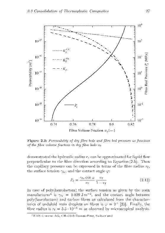
2.3 Consolidation of Thermoplastic Composites 27
r -. I I 1 / ' =
/ -
—~_
*"»«
^
-•*-*---- / \
lo-15
t'CK*» N /
X. • /
10"16Ap
jEl / V Z
4? -Kv / ^a
1ID"17
/ W :
X "* "
10-18
t0-19Y
Pt ill
;«:
m-2o /1
1 '_
1 1 1 1
0.74 0.76 0.78 0.8 0.82
Fibre Volume Fraction üf[—]
104
-. 10
10"
101
Ug
I'S
io° a
10"1
10""
Figure 2.3: Permeability of dry fibre beds and fibre bed pressure as function
of the fibre volume fraction m dry fibre beds vi.
demonstrated the hydraulic radius r\ can be approximated for liquid flow-
perpendicular to the fibre direction according to Equation (2.5). Then
the capillary pressure can be expressed in terms of the fibre radius rr,
the surface tension -nv, and the contact angle <p:
71v COS ip Vf
r-f 1 - Vf(2.13)
In case of poly(laurolactam) the surface tension as given by the resin
manufacturer4 is 7iv = 0.039 J m""2. and the contact angle between
poly(laurolactam) and carbon fibres as calculated from the character¬
istics of unduloid resin droplets on fibres is <p = 2° [35]. Finally, the
fibre radius is rf = 3.5 • 10""6 m as observed by microscopical analysis.
4EMS CriFMrE AG. CH 7013 Domat Ems. Switzerland
28 Consolidation of Commingled Yarns
Setting the fibre volume fraction to a representative value of Vf = 0.75. a
positive capillary pressure of Pr = 3 • 104 Pa is obtained.5 This pressure
is approximately two orders of magnitude lower than the usually appliedmechanical pressures. The capillary pressure is therefore considered to
be negligible. It is furthermore expected that, for polymer melts with
relatively low7 viscosities in unconfined environments, the pressure sup¬
ported by the matrix Pm is considerably lower than that carried by the
fibre network, and it is thus also neglected. Hence the total pressure
acting on the fibre bed is Pf = /a — I\. It is further assumed that the
air can leave the the fibre bed without being significantly pressuriseduntil a critical void radius r> is reached at which the pores are closed.
Subsequently, air pressure PY as a function of pore radius r is building
up as [30]:
f P0 if r > rc
IW = {D /rt^ (2.14)
IM7),fr<r^
where Pq is the ambient air pressure and rc is the critical void radius
at which the pore will be closed. Note that the so defined void pressure
represents a highly simplified model of the real void pressure evolution
during consolidation. There will be a critical pressure difference Pa — PY
at which a void of given radius will vanish. This can not be accounted
for with Equation 2.14 as infinitely small void radii yield infinite void
pressures. However, the present laminates cannot be expected to be free
of voids and thus the simple void pressure definition is a reasonably good
approximation. Bernet et al. [30] found that rc = 3.5 • 10~"5 in.
Having defined all parameters in Equation (2.2) the time necessary to
entirely impregnate a given fibre bed can—in principle—be computed.
However, Equation (2.2) does not account for entrapped voids and,
hence, it must be considered as a highly simplified description of real
fibre impregnation processes. Detailed analysis of impregnation mecha¬
nisms lead to the development of a number of consolidation models, some
of which are discussed in the next section, focusing on impregnation of
commingled yarn intermediate products.
5A positive \alue of the capillary pressure indicates that it enhances flow.
2.4 Impregnation Models for Commingled Yarns 29
2.4 Impregnation Models for CommingledYarns
Several models have been developed to predict the impregnation and
consolidation of commingled yarn composites [20, 30, 36 39] and some
of these are reviewed in [24].
The models generally predict the time to complete wetting and removal
of air voids—i.e., the times for iiiterfacial bonding and crystal formation
are not considered. If consolidation is assumed to take place simulta¬
neously in all fibre bundles, impregnation of only one of these bundles
needs to be considered. Geometrical relationships are then derived be¬
tween the unit cell dimensions and the total laminate thickness [36].
2.4.1 Modelling without Considering Fibre Bed Com¬
paction
Ye et al. [20] assume the following boundary conditions for their mod¬
elling:
• The shear rate is low so that Newtonian flow can be assumed and
the flow is laminar. This is valid for Reynolds numbers Re « 10""3.
• The impregnation into fibre tows is governed by Darcy's law
and the fibre tow permeability is a function of the fibre volume
fraction—i.e., the fibre spacing.
• Resin flow is transverse to the fibre direction.
« The applied pressure Pa is constant over the whole laminate area.
• Capillary effects and body forces such as gravity are considered to
be negligible.
® The bundle width b of the reinforcing fibres is constant and inde¬
pendent of the stage of impregnation.
The bundle width b is measured directly from the yarn, and the cross
sectional area At of a fully consolidated yarn is calculated from the
weight per unit length of the yarn W{ and the density of the consolidated
varn p:
At =^ (2.15)P
30 Consolidation of Commingled Yarns
Assuming that the yarn cross section is deformed to a rectangle due to
the applied pressure, the height ho of a fully consolidated yam is then
determined by:
h0 =y (2.16)
It is further assumed that the local fibre volume fraction is constant,
i.e., compaction is solely governed by the process of molten polymerflow into the reinforcing fibre bundles. In other words, the fibre volume
fraction in the dry fibre bed Vf equals the general fibre volume fraction Vf
of the fully consolidated composite. To ascertain smooth and consistent
representations of Ye's model Vf is replaced with the general fibre volume
fraction Vf for now. This assumption is very inaccurate and it will be
left out in subsequent models.
The rate of impregnation—i.e., the velocity of the flow front unq—isgiven by Darcy's law as presented in Equation (2.1) and the permeability
LCpK is calculated according to the Carman Kozeny equation as noted
in Equation (2.6). Solving Equation (2.1) for the flow front position x as
a function of time yields:
xmltp<±^l (2J7)V 2 iK vf
Here and henceforth the »--coordinate designates always the direction
transverse to the fibre axis if not mentioned otherwise. To calculate the
void content in relation to the flow7 front position a geometric parameter
C that depends on the degree of commingling (C = 0 for total segregationof polymer and reinforcement fibres, and C = 1 for perfect commingling)is introduced. The volume fraction of voids vv is then computed as:
Am-b{l-vt)(Cho + 2x(t))At + Am-b(\-vt)(Cho+2x(t))
where Am = (1 — Vf) At is the cross-sectional area covered by the matrix.
The thickness of the laminate h can be calculated as:
h = !^=jû (2.19)
where Nkl is the total number of fibre bundles in a laminate cross section
of height h and width W.
Although in some cases relatively good agreement between Ye's model
and experimental data was achieved, this approach has two serious draw¬
backs. One of them is the already mentioned assumption of constant
2.4 Impregnation Models for Commingled Yarns 31
fibre volume fraction and the other is in the commingling parameter C,which is difficult to determine other than by data fitting.
2.4.2 Modelling for Low Degree of Co-minglieg with
Fibre Bed Compaction
Van West ct al. [36] approached the problem in a different way. Theyobserved that in case of the investigated material the polymer fibres
tended to segregate and form a bundle of polymer fibres within the rein¬
forcement fibre bundles. The considered unit cell was therefore equal in
size to an entire yarn cross-section. The general model then incorporatesthree submodels:
• a compaction submodel, which predicts the change in thickness
with applied load of the fibre bed, excluding the matrix;
• a permeability submodel, which determines the bundle permeabil¬
ity given the instantaneous fibre volume fraction; and
® an impregnation submodel, which predicts the advancement of the
matrix flow front within the bundle.
The consolidation of a single bundle is assumed to be duplicated simul¬
taneously in all bundles. Geometric relationships exist between a unit
cell geometry and the total laminate thickness. These relationships are
useful in determining the laminate thickness from calculated unit cell
dimensions and vice versa at any stage during the consolidation process.
In Figure 2.22 the geometric relationships between cross sectional areas
and laminate thickness arc illustrated together with the nomenclature
used in this paragraph. Further to Figure rcfvanwestmodel the geomet¬
ric relationships are summarised in Table 2.2. The symbols 5b, «o. and
6o refer to the bundle spacing (i.e., the distance between neighbouringfibre bundles), and major and minor half axis length of the ellipsoidalfibre bundle cross sections, respectively.
To express the compaction of the fibre bed the model of Hou [40] was se¬
lected because it expresses compaction in terms of laminate thicknesses
rather than fibre diameter. Due to its three parameters that are eval¬
uated empirically, this model offers the necessary generality to fit the
experimental data for fabrics as well as layered fibre beds. Van West
et al. [36] modified the model to express it in terms of applied pressure

32 Consolidation of Commingled Yarns
r
B
=3a
<
©oocdA=A + An + A,
A, A=A + An
A = A + Ar. + Av
A A = A
4 = 4 + 4,+ An
\K A = A + A,
At : total unit cell area
4 : bundle area (including internal voids)
Ar : fibre area
Am : matrix area
Aey : external void area
4, : internal void area
ht : coalesced matrix thickness
hh : clustered bundle thickness
h^ : fully consolidated thickness
Figure 2.4: Cross-sectional area and laminate thickness relationships (after
Ref. [36]).
rather than force, and in terms of a minimum possible thickness rather
than a multiple of fibre radius and number of layers:
Kfh0
h0 - h
ho - hx
(2.20)
where Pf is again the pressure supported by the fibre network as in¬
troduced above, Kf is an elastic constant similar to that in Gutowski's
compaction model [29], ho is the initial laminate thickness prior to the
application of load, h^, is the minimum possible laminate thickness, h is
the instantaneous laminate thickness, and n is an exponent. The values

2.4 Impregnation Models for Commingled Yarns 33
Table 2.2: Calculation of cross-sectional areas and laminate thicknesses.
Parameter Geometric Relationship
Area of reinforcing fibres in a yarn
Area of matrix in a yarn
Area of reinforcing fibre bundle
Thickness at matrix coalescence
Clustered bundle thickness
Fully consolidated thickness
Fibre to non-fibre volume ratio
Fibre volume fraction8
"Other than the general fibre volume fraetion i/j of the thoroughly consolidated
laminate, the present volume fraction ij{ depends on the state of consolidation
Ar = Af7rrr2
An = At(±- l)1 TTOo&O for
" b ~
\ Sh^r for
h > /ib
h < hb
h = (Ab + Am)^hb = Ab£hc = At^r-
4 AtA -
At,-At
of Kf, ft-oo, and n are found empirically. Van West et al. [36] employed the
modified Carman Kozeny equation proposed by Gutowski et al. [29] to
describe the permeability of the fibre bundles K^iu as a function of the
instantaneous fibre volume fraction Vf and fibre radius as given presentedin Equation (2.7).
For the impregnation submodel it is assumed that the fibre bundles
undergo impregnation simultaneously and their cross-sectional area is
contained within an ellipse of equal major and minor half-axis length
ao and bo for all bundles. Hence, it is sufficient to analyse one bun¬
dle to obtain the behaviour of the entire laminate. Due to the lack of
rotational symmetry of the elliptical geometry the problem would have
to be treated in to dimensions. This w7as, however, circumvented by
numerically determining a relationship between an elliptical fibre bun¬
dle and an equivalent circular fibre bundle so that both have the same
impregnation time. This approach simplifies the impregnation problemof elliptical fibre bundles to a one dimensional analysis in polar coordi¬
nates. The relationship between the ellipse's major and minor half axis
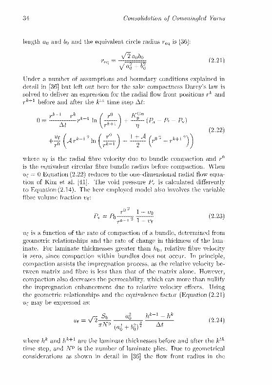
34 Consolidation of Commingled Yarns
length ao and bo and the equivalent circle radius req is [36]:
(2.21)
Under a number of assumptions and boundary conditions explained in
detail in [36] but left out here for the sake compactness Darcy's law is
solved to deliver an expression for the radial flow front positions rk and
rfe-T-i Defore arK] after the kth time step Ar:
°=LV1'J'+'l"fe)+ir</ww''
<l(A^'*(£)-1±* {<"-'"")(2.22)
where Uf is the radial fibre velocity due to bundle compaction and r°
is the equivalent circular fibre bundle radius before compaction. When
Uf = 0 Equation (2.22) reduces to the one dimensional radial flow equa¬
tion of Kim et al. [41]. The void pressure Pv is calculated differentlyto Equation (2.14). The here employed model also involves the variable
fibre volume fraction vf.
Uf is a function of the rate of compaction of a bundle, determined from
geometric relationships and the rate of change in thickness of the lam¬
inate. For laminate thicknesses greater than h\>, relative fibre velocityis zero, since compaction within bundles does not occur. In principle,
compaction assists the impregnation process, as the relative velocity be¬
tween matrix and fibre is less than that of the matrix alone. However,
compaction also decreases the permeability, which can more than nullify
the impregnation enhancement due to relative velocity effects. Usingthe geometric relationships and the equivalence factor (Equation (2.21)Uf may be expressed as:
Uf = V2^- °° /*+1-** (2.24)
where hk and hk+1 are the laminate thicknesses before and after the kth
time step, and A'p is the number of laminate plies. Due to geometricalconsiderations as shown in detail in [36] the flow front radius in the
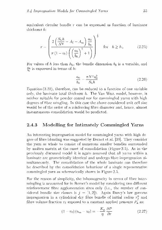
2.4 Impregnation Models for Commingled Yarns 35
equivalent circular bundle r can be expressed as function of laminate
thickness h:
for ft > ftb (2.25)
For values of ft less than hi,, the bundle dimension 6q is a variable, and
f1 is expressed in terms of ft:
«o=
îrA^ogbo S\}h
Equation (2.22), therefore, can be reduced to a function of one variable
only, the laminate total thickness h. The Van West model, however, is
neither suitable for powder coated nor for commingled yarns with high
degrees of fibre mingling. In this case the above considered unit cell size
would be of the order of a reinforcing fibre diameter and, hence, almost
instantaneous consolidation would be predicted.
2.4.3 Modelling for Intimately Commingled Yarns
An interesting impregnation model for commingled yarns with high de¬
gree of fibre blending was suggested by Bernet et al. [30]. They consider
the yarn as whole to consist of numerous smaller bundles surrounded
by molten matrix at the onset of consolidation (Figure 2.5). As in the
previously discussed model it is again assumed that all yarns within a
laminate are geometrically identical and undergo fibre impregnation si¬
multaneously. The consolidation of the whole laminate can therefore
be described by the consolidation behaviour of a single representative
commingled yarn as schematically shown in Figure 2.5.
For the reason of simplicity, the inhomogciieity in terms of fibre inter¬
mingling is accounted for in Bernet's model by considering twro different
reinforcement fibre agglomeration sizes only (i.e., the number of con¬
sidered bundle size classes is j = [1,2]). Again Darcy's law governs
impregnation in a cylindrical dry fibre bundle of initial radius r() and
fibre volume fraction Vf exposed to a constant applied pressure Ptl as:
(l-Uf)(«m-«f) = -^Ji^ (2-27)n or

36 Consolidation of Commingled Yarns
Onset of yarn
consolidation
Impregnation of
fibre bundles
Full yarn
consolidation
Figure 2.5: Schematic of a representative yarn cross-section and consolida¬
tion process (after Ref. [30]).
where um and Uf are the matrix and fibre velocities, respectively, and P
is the local pressure—i.e., at the instantaneous radial flow front position
r.
Continuity equations for solid and liquid phase within a representativevolume element AV", which is small enough to consider average values
within this element, yield:
dvt do (2.28)
ö(l- Vf) d, ,
where t is the impregnation time.
Finally, a stress equilibrium equation is written:
OP
8r
d(Tf
"~d7
(2.29)
(2.30)
where Of is the effective stress tensor component in radial direction expe¬
rienced by the fibre network, which is counted as positive in compressionand is a function of i>f. Two simplifying assumptions arc made:
« resin flow only takes place in radial fibre bundle direction, i.e.,
orthogonal to the fibre axis.
• once the fibre bed is compressed, a change in local pressure does
not create a significant change in volume fraction, and thus the
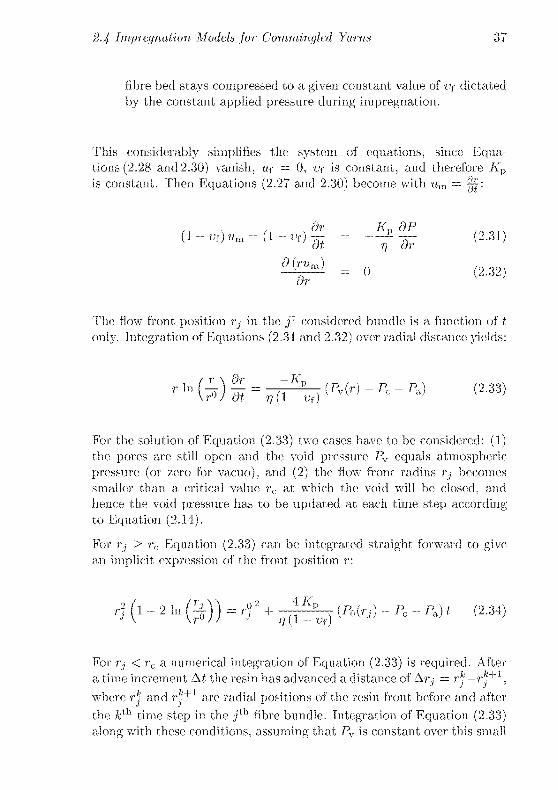
2.4 Impregnation Models for Commingled Yarns 37
fibre bed stays compressed to a given constant value of Vf dictated
by the constant applied pressure during impregnation.
This considerably simplifies the system of equations, since Equa¬tions (2.28 and 2.30) vanish, Uf = 0, Vf is constant, and therefore Kpis constant. Then Equations (2.27 and 2.30) become with Mm = |~:
(l-vt)nm = (l-vt)% = -^-^f- (2.31)dt n dr
d{rum)Or
(2.32)
The flow front position rj in the f considered bundle is a function of t
only. Integration of Equations (2.31 and 2.32) over radial distance yields:
'"(?) 7g = „A'Aip--<rl-fi-p"> (133>at r}{\ - Vf)
For the solution of Equation (2.33) two cases have to be considered: (1)the pores arc still open and the void pressure 1\ equals atmospheric
pressure (or zero for vacuo), and (2) the flow front radius rj becomes
smaller than a critical value rc at which the void will be closed, and
hence the void pressure has to be updated at each time step accordingto Equation (2.14).
For rj > rc Equation (2.33) can be integrated straight forward to givean implicit expression of the front position r:
l21K^))=rf + ^fe^^^/^i^t (2-M)
For rj < rc a numerical integration of Equation (2.33) is required. After
a time increment At the resin has advanced a distance of Arj = r* —r*+ '.
where rk and rk+1 are radial positions of the resin front before and after
the kih time step in the jth fibre bundle. Integration of Equation (2.33)along with these conditions, assuming that Pv is constant over this small

38 Consolidation of Commingled Yarns
increment, yields:
At =rj(l~Uf)
MPa + Pc-PvCT1))
(2.35)
Once the position of the front is known for a given bundle at a given time,
this value needs to be related to the macroscopic void content within a
yarn. For this, the yarn is assumed to be constituted of a distribution
of n different bundle sizes, a size group j containing Ara bundles, each of
initial radius r° and comprising <Vf fibres. The initial void radius equalsthe size of a diy fibre bundle, which is determined by the number of
Nlr'2
rf =^ (2.36)
Vi
Then, the total volume fraction of voids within the commingled yarn,
vY, is:n
1
E-^-rro^)
!/, = -^ (2.37)
A+J2N*(r^)2(l~Uf)j-i
where At is the cross-sectional area of an entiielv consolidated commin¬
gled yarn. It is easily deteimined as:
At = ^± (2.38)Vf
where Nt is the total number of reinfoi cing fibres in the total commingled
yarn, i.e., ArT = Yll-i ^Y^Y?' and vf lb a8am tne general fibre volume
fraction of the total fullv consolidated yarn.
Combining Equation (2.37) with Equations (2.34 and 2.35) allows for
predicting the void content of the commingled yarn, and thus the lami¬
nate, at each time step during consolidation. If this model as applied for
2.4 References 39
non isothermal processes such as stamp forming the solution methodol¬
ogy remains the same but the resin viscosity has to be updated at each
time increment.
Bernet et al. [30] used a commingled yarn product with relatively high
degree of fibre blending with a general fibre volume fraction Vf of 0.56 for
experimental validation of their model. Although this yarn exhibits good
commingling quality, a few large fibre agglomerations where A"r = 225
and numerous small agglomerations of ATf = 50 were observed. Only
these two agglomeration sizes multiplied with their respective frequen¬cies were then used to calculate the void content according to Equa¬tion (2.37). Despite this simplification Bernet ct al. [30] achieved excel¬
lent agreement between computed and measured void contents.
The validity of Bernet's model for extremely good blending quality, i.e.,
very small fibre bundles, will be discussed in Chapters 5 and 6. To obtain
more general validity of the model, however, the fibre agglomeration size
is here treated as a statistical quantity. The frequency of occurrence of
a given agglomeration size O is assumed to obey a logarithmic normal
distribution with variance s'2 and predictand /t* = (In (A'"j)):
References
[1] A. E. Scbeideggcr. The Physics of Flow Through Porous Media.
University of Toronto Press, 3rd edition, 1974.
[2] D. C. Leach. Continuous Fibre Reinforced Thermoplastic Matrix
Composites. In T. K. Partridge, editor, Advanced Composites, chap¬ter 2, pages 43 109. Elsevier Sei. Pub. LTD. Essex, UK. 1989.
[3] P. A. Hogan. The production and uses of film stacked composites
for the aerospace industry. In 14th SAMPE Technical Conference,New York, 1980.
[4] U. Measuria and F. N. Cogswell. Thermoplastic composites in wo¬
ven fabric form. In IMechE. 1986. paper C21.

40 Consolidation of Commingled Yarns
[5] D. M. Bigg. Processing characteristics of thermoplastic sheet com¬
posites. International Polymer Processing. VTT:172 185, 1992.
[6] E. M. Silverman and R. J. Jones. Property, processing and perfor¬mance of graphite/PEEK prepreg tape and fabrics. SAMPE Jour¬
nal, 24(4):33 40, 1988.
[7] B. Varughese, J. Muzzy, and R. M. Baucom. Combining LaRC TPT
powder with carbon fiber by electrostatic fluidized bed coating. In
Proceedings of the 21st International SAMPE Technical Conference,
pages 536 543. Atlantic City, USA, 1989.
[8] J. M. Marchello and R. M. Baucom. LaRC dry powder towpreg pro¬
cess. In Proceedings of the 36th International SAMPE Symposium.
pages 68-80, Anaheim, USA, 1991.
[9] AI. K. Hugh, J. M. Marchello. R. M. Baucom, and N. J. Johnston.
Composites from powder coated towpreg. Studies with variable tow
sizes. In Proceedings of the 37th International SAMPE Symposium,
pages 1040-1051, Anaheim, USA, 1992.
[10] A. AI. Vodermaycr. J. C. Kaerger, and G. Hinrichsen. Manufac¬
ture of high performance fibre-reinforced thermoplastics by aqueous
powder impregnateion. Composites Manufacturing. 4(3):123-132,1993.
[11] B. W. Gantt, D. D. Edie, G. C. Lickficld, M. J. Drews, and M. S.
Ellison. Thermoplastic coating of carbon fibers. In ASTM Sympo¬sium on Advances in Thermoplastic Matrix Composite Materials,Bal Harbour, USA. 1987.
[12] S. R. Clemans, E. D. Western, and A. C. Haiidermann. Hybrid
yarns for high performance thermoplastic matrix composites. In
J. de Bossu, G. Briens, and P. Lissac, editors, Looking Ahead forMaterials and Processes, pages 429 434. Elsevier Science Publish¬
ers, Amsterdam, 1987.
[13] M. E. Ketterer. Thermoplastic/carbon fiber hybrid yarn. Contrac¬
tor Report 3849, NASA, 1984.
[14] M. Acar. Air jet textured products for technical and industrial
use. In Proceedings of Techtext.il Symposium, pages 1 7, Frankfurt.
Germany, 1990.

2.4 References 41
[15] L. Long, Y. Jianyong, and W. Shanyuan. Alechanical properties of
air jet commingled yarn composites. SAMPE Journal, 33(6):29 31,
1997.
[16] G. Roncato, R. Fedorowsky. P. Boissonnat, and D. Boubinoux. Dis¬
positif de fabrication d'un fil composite formé de fibres de renforce¬
ment et de matière orgnaique thermoplastiqe. European Patent,No. 0505274, 1992.
[17] G. Roncato. R. Fedorowsky, P. Boissonnat. and D. Boubinoux.
Procédé et dispositif de fabrication d'un fil composite. European
Patent, No. 0505275. 1992.
[18] N. Bernet. Commingled Yam Composites For Rapid Processing of
complex Shapes. PhD thesis. Swiss Federal Institute of Technology,2000. Diss. EPFL No. 2154.
[19] R. Phillips. D. A. Akyiiz, and J.-A. E. Alânson. Compressibilityand relaxation of fiber reinforcements dring composite processing,
part i. isothermal case. Composites. Part A: Applied Science and
Manufacturing, 29A(4):395-402, 1998.
[20] L. Ye, K. Friedrich, J. Kastei, and Y.-W. Alai. Consolidation of
unidirectional cf/peek composites from commingled yarn preprcg.
Composites Science and Technology, 54(4):349-358, 1995.
[21] L. Ye, V. Klinkmüller, and K. Friedrich. Impregnation and consol¬
idation in composites made of gf/pp powder impregnated bundles.
Jorunal of Thermoplastic Composite Materials. 5:32 48. 1992.
[22] M. Connor, S. Toll, J.-A. E. Malison, and A. G. Gibson. A
model for the consolidation of aligned thermoplastic powder impreg¬nated composites. Journal of Thermoplastic Composite Materials,
8(2):138 162. 1995.
[23] M. Connor. Consolidation Mechanisms and Interfacial Phenom¬
ena in Thermoplastic Powder Impregnated Composites. PhD thesis.
Swiss Federal Institute of Technology, Lausanne. Switzerland, 1995.
Diss. EPFL No. 1413.
[24] N. Svensson and R. Shishoo. Manufacturing of thermoplastic com¬
posites from commingled yarns a review. Journal of Thermoplastic
Composite Materials, 11:22 56. 1998.
42 Consolidation of Commingled Yarns
[25] C. E. Carraher, Jr. Seymour/Carraher's Polymer Chemistry, An
Introduction. Marcel Dekker, Inc., New York, 4th edition. 1996.
[26] C. Baron, F.-E. Baumann, H. Dacbel, J. Aliigge, and U. Rohde-
Liebenau. Polyamid 11 und 12. In L. Bottenbruch and R. Bin-
sack, editors, Kunststoff-Handbuch, 3(4): Technische Thermo¬
plaste, Polyamide, chapter 4, page 723. Hanser Verlag, München,1999.
[27] P. C. Carman. Fluid flow through a granular bed. Transactions ofthe Institution of Chemical Engineers, 15:150-167, 1937.
[28] K. J. Ahn, J. C. Seferis. and J. C. Berg. Simultaneous measurements
of permeability and capillary pressure of thermosetting matrices in
woven fabric reinforcements. Polymer Composites, 12(3): 146 152.
1991.
[29] T. G. Gutowski. Z. Cai. S. Bauer. D. Boucher. J. Kingery, and
S. Wineman. Consolidation experiments for laminate composites.Journal of Composite Materials, 21(7):650 669, 1987.
[30] X. Bernet, V. Michaud, P.-E. Bourban. and J.-A. E. Alânson. An
impregnation model for the consolidation of thermoplastic compos¬
ites made from commingled yarns. Journal of Composite Materials,
33(8):751 772, 1999.
[31] B. R. Gebart. Permeability of unidirectional reinforcements for rtm.
Journal of Composite Materials, 26(8):1100-1133, 1992.
[32] T. G. Gutowski. A resin flow/fiber deformation model for compos¬
ites. SAMPE Quarterly, 16(4):58 64, 1985.
[33] T. G. Gutowski, J. Kingery, and D. Boucher. Experiments on com¬
posites consolidation: Fiber deformation. In ANTEC'86, pages
1316 1320,1986.
[34] T. G. Gutowski, Z. Cai, J. Kingery, and S. Wineman. Resin
flow/fiber deformation experiments. SAMPE Quarterly, 17(4):54-58, 1986.
[35] II. D. Wagner. Spreading of liquid droplets on cylindrical sur¬
faces: Accurate determination of contact angle. Journal of Applied
Physics. 67(3): 1352 1355,1990.

2.4 References 43
[36] B. P. Van West. R. B. Pipes, and S. G. Advani. The consolida¬
tion of unidirectional CF/PEEK composites from commingled yarn
prepreg. Polymer Composites, 12(6):417 427, 1991.
[37] Y. Klinkmüllcr, M. K. Um, K. Friedrich, and B.-S. Kim. A new
model for impregnation mechanisms in different gf/pp commingled
yarns. Applied Composite Materials. 1:351 371, 1995.
[38] L. Ye. K. Friedrich, and J. Kastei. Consolidation of gf/pp com¬
mingled yarn composites. Applied Composite Materials. 1:415-429,1995.
[39] T. A. Cain, AL D. Wakeman, R. Brooks, A. C. Long, and C. D.
Rudd. Towards an integrated processing model for a co mingled
thermoplastic composite. In Proceedings of the 1 tth International
Conference on Composite Materials, volume V, pages 366 376, Gold
Coast, Australia, 1997.
[40] T. IL Hou. A resin flow model for composite prepreg laminate
process. In Proceedings of the Society of Plastics Engineers. 44thAnnual Technical Conference, pages 1300 1305, Boston, L'SA, 1986.
[41] T. W. Kim, E. J. Jun, and W. I. Lee. Compaction behavior of thick
composite laminates during cure. In G.A. Zakrzewski. editor, 34thInternational SAMPE Symposium, volume 1, pages 15-19, Reno,Ncvad. USA, 1989.

44 Consolidation of Commingled Yarns

Chapter 3
Parameters for Thermal
Calculations
In prospect of Chapters 4 and 6. where the temperature evolution of
commingled yarn fabric stacks during beating and of laminates during
consolidation/cooling will be investigated, material parameters used for
thermal calculations and their variation with temperature, and in some
cases also pressure are discussed. Additionally to the material parame¬
ters of the laminate, numeric values are also given for poly(ethcr-ether-ketonc) (PEEK), since the moulding tool for heat transfer experiments
during stamp forming are machined from this material.
3.1 Differential Scanning Calorimetry
DSC analysis was employed to measure the latent heat of crystallisationof PA-12 as well as the specific heat of PA-12, PEEK, carbon fibres, and
carbon fibrc/PA-12 laminate containing 50 % carbon fibres by volume.
DSC measurements were performed using a Per kin Elmer Pyris 1
DSC, with the block held at —196 °C.The measurement cell was purged
with dry Helium at a flow rate of 1.2 ml s_1. All samples were embedded
in aluminium pans without covers. The specific beat of PA 12 melts be¬
tween 180 °C and 240 °C was measured using the same sample geometry.
The sample was heated to 240 °C.where it was held for 2 min, and then
cooled to 180 °C at f °C s_1. where it was again held for 2 min. As the
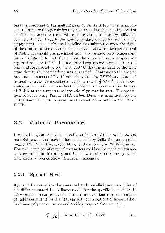
46 Parameters for Thermal Calculations
onset temperature of the melting peak of PA 12 is 178 °C, it is impor¬
tant to measure the specific heat by cooling rather than heating, so that
specific heat values at temperatures close to the onset of crystallisation
can be obtained. Exactly the same procedure was performed with two
empty pans. The so obtained baseline was subtracted from the signalof the sample to calculate the specific heat. Likewise, the specific heat
of PEEK the mould was machined from was assessed on a temperature
interval of 35 °C to 140 °C. avoiding the glass transition temperature
reported to be at 147 °C [1]. In a second experiment carried out on the
temperature interval of 100 °C to 200 °C the contribution of the glasstransition to the specific heat was quantified. Contrary to the specificheat measurements of PA 12 melt the values for PEEK were obtained
by heating rather than cooling at a cooling rate of | °C s""1, as the above
stated problem of the latent heat of fusion is of no concern in the case
of PEEK at the temperature intervals of present interest. The specificheat of about 5 mg Tenax HTA carbon fibres was measured between
100 °C and 200 °C, employing the same method as used for PA-12 and
PEEK.
3.2 Material Parameters
It was taken great care to empirically verify some of the more importantmaterial parameters such as latent heat of crystallisation and specificheat of PA-12, PEEK, carbon fibres, and carbon fibre PA-12 laminate.
However, a number of material parameters could not be made experimen¬
tally accessible in this study, and thus it was relied on values provided
by material suppliers and/or literature references.
3.2.1 Specific Heat
Figure 3.1 summarises the measured and modelled heat capacities of
the different materials. A linear model for the specific heat of PA-12
c versus temperature can be assumed in accordance with an empiri¬cal addition scheme for the heat capacity contributions of linear carbon
backbone polymer segments and amide groups as shown in [2, 3].
cp [pc] = 4-04 " 10_3T tK] + °-856 (3-1)
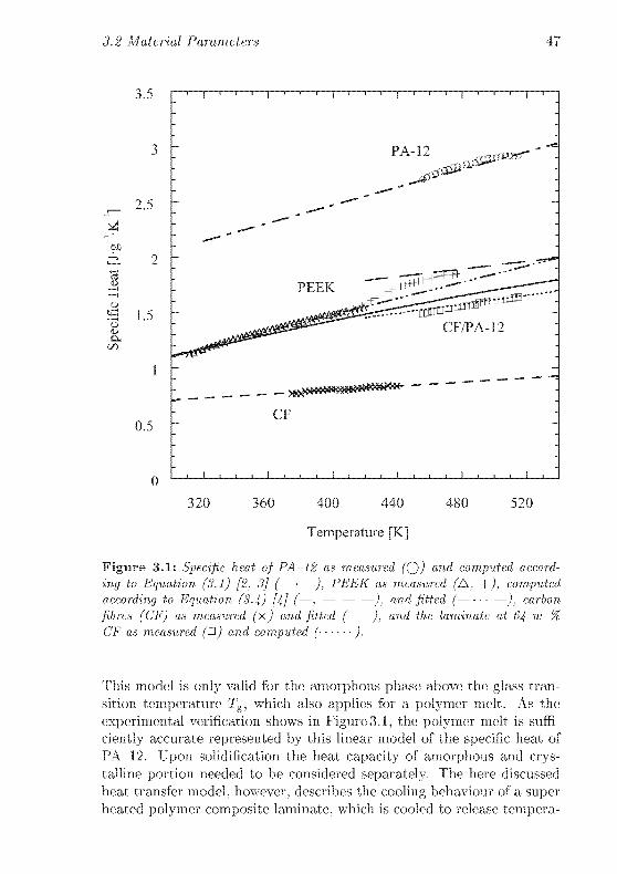
3.2 Material Parameters 47
3.5
2.5-
0.5
~j i ! 1 \ 1 i 1 1 1 1 ! 1 ! 1 i j i ! 1 |~
PA-12
CF/PA-12
CF
I i I i I \ I I i t S t I i I i I \ I
320 360 400 440
Temperature [K]
480 520
Figure 3.1: Specific heat of PA 12 as measured (Ç)) and computed accord¬
ing to Equation (3.1) [2, 3] ( ), PEEK as measured (A. +), computed
according to Equation (3.4) [4] (—; — — —), o,nd fitted (— • • —), carbon
fibres (CF) as measured (x) and fitted ( ), and the laminate at 64 w-%
CF as measured (a) and computed ( ).
This model is only valid for the amorphous phase above the glass tran¬
sition temperature Tg, which also applies for a polymer melt. As the
experimental verification shows in Figure 3.1, the polymer melt is suffi¬
ciently accurate represented by this linear model of the specific heat of
PA 12. Upon solidification the heat capacity of amorphous and crys¬
talline portion needed to be considered separately. The here discussed
heat transfer model, however, describes the cooling behaviour of a super
heated polymer composite laminate, which is cooled to release tempera-

48 Parameters for Thermal Calculations
ture under static pressure. The release temperature is thereby well above
Tg of PA 12, which is at 314K [5]. Hence, the above presented linear
model for the specific heat of the polymer would be valid throughoutthe whole temperature interval considered here if the sample was en¬
tirely amorphous. As the crystallisation temperature is here relativelyclose to the release temperature it is justified to neglect the slight changeof specific heat due to the crystallised portion of the polymer.The measured specific heat data of carbon fibres was subjected to a lin¬
ear fit and it was found that extrapolation to 300 K delivers a cp value
of 0.71 Jg_1 K""1, which agrees with the value provided by the material
supplier at 293 K.
cP [^] = 9.17 - 10~4T [K] + 0.435 (3.2)
From the fit to the data of carbon fibres and the linear model for neat
PA-12 the specific heat of the laminate can be calculated by addition,
taking the weight fraction of each component into account.
= 2.04 • 10-3T [K] + 0.586
where Wf is the mass fraction of carbon fibres in the void free laminate.
The contribution of air to the total specific heat is not accounted for as
the mass fraction of air is extremely small due to its low density.
Specific heat measurements of PEEK agree well with the data calculated
by Varma-Nair and Wunderlich [6] at temperatures lower than Tg. The
model developed by Varma-Nair and Wunderlich does not account for
the change in cp involved with the phase transformation. In an ear¬
lier publication, Cheng and Wunderlich [4] proposed a linear approach,to calculate the beat capacity of entirely amorphous PEEK above Tg.The here measured data recorded on a temperature interval that con¬
tains Tg approaches the calculated specific heat of amorphous PEEK.
To maintain a simple linear relationship between cp and temperature
the following equation was implemented in the thermal model:
êp[pc] = 3.70 • 10-Jr[K] (3.4)

3.2 Material Parameters 49
3.2.2 Latent Heat of Crystallisation, Crystallisation
Temperature, and Degree of Crystallinity
Several material parameters such as the laminate density and thermal
conductivity distinctly change as the liquid/solid phase change happensto begin. Hence, the computer program that contains the thermal model
permanently checks the present cooling rate and laminate temperatures
and sees to whether or not Equation (6.11) is fulfilled. If so, the pro¬
gram switches from the parameter set given for the polymer melt to the
corresponding functions determined for the solid polymer.
The total degree of crystallinity was determined by density measure¬
ments and reference data of amorphous and crystalline PA 12 densities
rather than by comparison of the latent beat of crystallisation with the
theoretic value for a perfect polymer crystal. As stated above the latent
heat of crystallisation is not significantly affected by cooling rate up to
1.5 °Cs_l. Hence, the degree of crystallinity is assumed to stay ap¬
proximately constant within the considered range of cooling rates. The
density of extruded granules was thus taken to be representative for the
crystallinity calculation. According to the literature the densities of the
amorphous and crystalline phase amount to 1.048 and 0.990 g cm""3, re¬
spectively [7, 8]. The density of PA 12 granules was measured to equal
l.OlOgcm""3, yielding an absolute crystalline volume fraction of 0.34.
3.2.3 Thermal Conductivity
The thermal conductivity Am of EMS Chemie Grilamid LI 6 PA 12
is 0.25 Wm"1 K"1 at 273 K as reported by the material supplier. Ac¬
cording to [9] the general shape of the Am vs. temperature curve can
be assumed to be similar for PA-6 and PA-12, although the change of
conductivity occurring at the phase transformation is not as dramatic
for PA-12 as for PA-6, which is attributed to the smaller affinity to
water absorption of PA-12. A thermal conductivity of 0.22 Win""1 K""1
is assumed for both the PA 6 and PA 12 melts. With these parameters
an approximated Am vs. temperature curve can be constructed for PA
12. The assumed temperature dependence of the thermal conductivity
of PA 12 along with data for PA-6 as reported by Throne and Beine [10]is shown in Figure 3.2. In the here presented thermal model the thermal
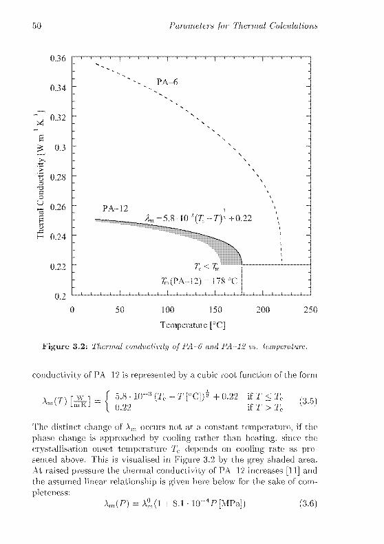
50 Parameters for Thermal Calculations
Q 36 !—'—'—'—'—!—'—!—'—'—!—'—'—!—!—i—'—'—'—'—!—!—'—'—1~
0.34
ï 0-32 :
T
s
Ë °-3 :
f'I 0.28
•§d
É 0.26
H 0.24
0.22
0.2
PA-12
PA-6
im=5.8-103(rc-r)3 +0.22
Tc < Tm
Î11(PA-12) = 178°C
_J I ! ! i I I I I ! ! I I I ! I L_ J I I ! L_
50 100 150
Temperature [°CJ
200 250
Figure 3.2: Thermal conductivity of PA 6 and PA 12 vs. temperature.
conductivity of PA 12 is represented bv a cubic root function of the form
5.8- 10""3(TC -T[°C]p +0.22 if T < T(_ven
[^
iïïïcJ0.22 if T > Tt
(3.5)
The distinct change of Am occurs not at a constant temperature, if the
phase change is approached by cooling rather than heating, since the
crystallisation onset temperature Tc depends on cooling rate as pre¬
sented above. This is visualised in Figure 3.2 bv the grey shaded area.
At raised pressure the thermal conductivity of PA 12 increases [11] and
the assumed linear relationship is given here below for the sake of com¬
pleteness:
A„,(P) = A°,(l +8.1 104P[AlPa]) (3.6)
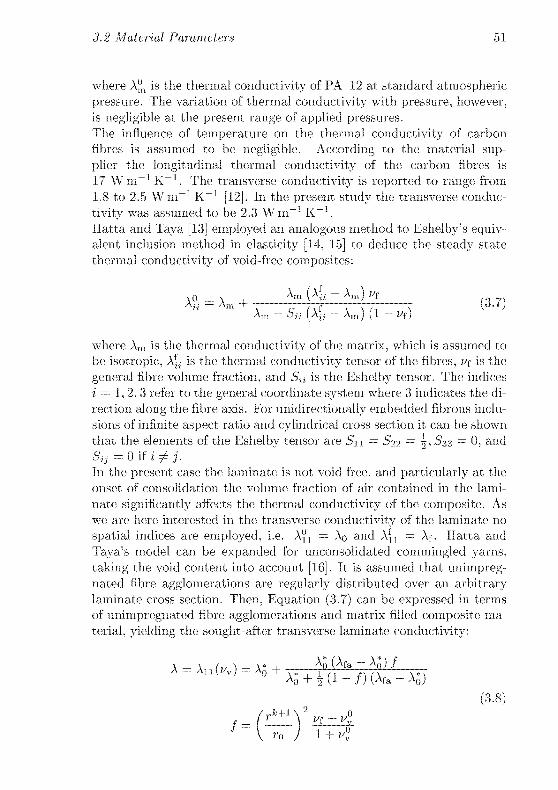
3.2 Material Parameters 51
where A", is the thermal conductivity of PA 12 at standard atmospheric
pressure. The variation of thermal conductivity with pressure, however,
is negligible at the present range of applied pressures.
The influence of temperature on the thermal conductivity of carbon
fibres is assumed to be negligible. According to the material sup¬
plier the longitudinal thermal conductivity of the carbon fibres is
17 Win""1 K~~'. The transverse conductivity is reported to range from
1.8 to 2.5 Win""1 K""1 [12]. In the present study the transverse conduc¬
tivity was assumed to be 2.3 Wm~~' K~~'.
Hatta and Taya [13] employed an analogous method to Eshclby's equiv¬alent inclusion method in elasticity [14, 15] to deduce the steady state
thermal conductivity of void-free composites:
A° = Am +Am ffi ~~ Xm] Vt
(3.7)
where Am is the thermal conductivity of the matrix, which is assumed to
be isotropic. A^ is the thermal conductivity tensor of the fibres, Vf is the
general fibre volume fraction, and S,j is the Eshelby tensor. The indices
i = 1,2,3 refer to the general coordinate system where 3 indicates the di¬
rection along the fibre axis. For unidirectionally embedded fibrous inclu¬
sions of infinite aspect ratio and cylindrical cross section it can be shown
that the elements of the Eshelbv tensor are Su = S22 = \, -S33 = 0, and
Szj = 0 if i jtj.In the present case the laminate is not void free, and particularly at the
onset of consolidation the volume fraction of air contained in the lami¬
nate significantly affects the thermal conductivity of the composite. As
we are here interested in the transverse conductivity of the laminate no
spatial indices are employed, i.e. A1^ = Aq and A'n = Af. Hatta and
Taya's model can be expanded for unconsolidated commingled yarns,
taking the void content into account [16]. It is assumed that unimpreg-nated fibre agglomerations are regularly distributed over an arbitrarylaminate cross section. Then. Equation (3.7) can be expressed in terms
of unimpregnated fibre agglomerations and matrix filled composite ma¬
terial, yielding the sought-after transverse laminate conductivity:
(3.8)

52 Parameters for Thermal Calculations
where Ai i (i/v) is the transverse thermal conductivity of the compositelaminate as a function of void content vv, Ag is the transverse ther¬
mal conductivity of already impregnated portions of the laminate (theasterisk is thought to remind the reader that the thermal conductiv¬
ity of impregnated fibres as noted in Equation (3.7) X^ is not equalto the present conductivity Aq, since the fibre volume fraction is not
constant but depends on the variation of void fraction), Afa is the trans¬
verse thermal conductivity of dry fibre agglomerations, and / is a factor
that expresses the volume fraction of matrix filled sections and dry fi¬
bre agglomerations in terms of the instantaneous and initial void radii
r*""1 and ro, and the initial void content i/°. Rather than evaluating
Equation (3.8) separately for each considered fibre agglomeration size as
given by r*"1"1, average values for both the inital and present void radii
are employed here.
Equation (3.8) is in principle the same as Equation (3.7) but combines
two material systems each containing two phases polymer and rein¬
forcement fibres as well as air and reinforcement fibres to give an ex¬
pression for the combined thermal conductivity of a three phase material
system, consisting of polymer, air. and reinforcement fibres. Thus, the
transverse thermal conductivities of matrix filled portions and dry fibre
agglomerations can be calculated employing Equation (3.7), replacingthe thermal conductivities of pure fibres and polymer by the transverse
conductivities of dry fibre agglomeration and polymer impregnated fi¬
bres, which can also be calculated in analogy to Equation (3.7):
\f -\,. .AAir (Af - A,Vir) Vî
fa " Air +
AAir + |(1- vt) (Ar - AAir)
\o«_
\ jAm (Af — Am) g
11 m +Am + i(l-ff)(Af-Am) (3-9)
where AA;r is the thermal conductivity of air, Vf is the fibre volume
fraction of a dry fibre agglomeration, and g is a factor that relates the
local fibre volume fraction of matrix filled areas with the composite's
general fibre volume fraction Vf. Due to the thermal conductivity of air
being five orders of magnitude smaller than the transverse conductivity

3.2 Material Parameters 53
of carbon fibres Afa simplifies to:
AAir VfAfa — AAir +
è(l-«r)
The fibre volume fraction of dry fibre agglomerations depends on the
difference between applied processing pressure Pa and void pressure Pv
to result in a fibre bed pressure Pf = Pa — Pv and can be expressed
according to Gutowski ct al [17] as presented in the previous chapter,
Equation (2.10) on page 26. If no or only a small pressure is applied to a
stack of fabric plies—as it will be the case in the Chapter 4—this can be
neglegcted and the fibre volume fraction assumes a constant value. In
Chapter 6, where the heat transfer of a laminate during stamp forming is
investigated, variations of fibre volume fraction in unimpregnated fibre
areas also have to be considered. One of the problems there is that
the air pressure of an entrapped void increases as the diameter of the
pore decreases according to Equation (2.14), and hence the fibre bed
pressure is not constant either. It is therefore pointed out here that
the reader may pay attention to the two different symbols referring to
general (constant) laminate fibre volume fraction Vf and variable fibre
volume fraction in uiiimprcgnated areas Vf, respectively.
3.2.4 Specific Volume
Most of the here below presented relationships refer to specific volume
rather than density, although density alterations due to variation of am¬
bient conditions are of particular interest in the present case. Densityand specific volume, however, have to be understood as interchangeable
parameters, where the former is the reciprocal value of the latter and
vice versa.
The specific volume of semicrystalline polymers depends on tempera¬
ture, pressure and—in the solid state—on crystallinity. The specificvolume of amorphous and crystalline PA-12 at 25 °C and a pressure of
4 MPa is 0.997 cm3g~"' and 0.949 crrr^g"1, and the corresponding vol¬
ume expansion coefficients equal 6.00 • 10""4 "C""1 and 7.89 • 10""5 °C_I,respectively. These numbers were obtained by adapting data reportedin [18] to the present level of applied pressure. Separation of amorphousand crystalline contributions was performed by calculation of the crys¬
talline volume fraction by means of the density at 25 °C and atmospheric
pressure as noted in [18] and the densities of amorphous and crystalline
phases according to [7. 8]. As soon as crystallisation onset is observed.
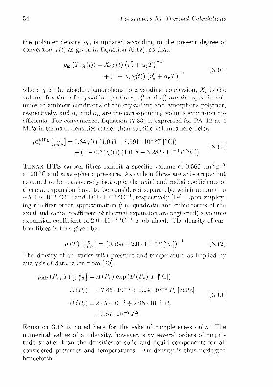
54 Parameters for Thermal Calculations
the polymer density pm is updated according to the present degree of
conversion \(t) as given in Equation (6.12), so that:
Pnl (T. x(t)) = XcX(t) (4' + acT)-1
+ (l-A'cx(r))K + aaï')"'
where \ ig the absolute amorphous to crystalline conversion, Xc is the
volume fraction of crystalline portions, v° and v® are the specific vol¬
umes at ambient conditions of the crystalline and amorphous polymer,
respectively, and qc and aa arc the corresponding volume expansion co¬
efficients. For convenience, Equation (7.33) is expressed for PA-12 at 4
AlPa in terms of densities rather than specific volumes here below:
/4MPa [^r] = 0.34A<(*) (1.056 - 8.591 • 10"5T [°C])+ (1 - 0.34x(0) (1.018 - 5.282 • W"4T [°C])
Tenax HTS carbon fibres exhibit a specific volume of 0.565 cm3g-1at 20 °C and atmospheric pressure. As carbon fibres are anisotropic but
assumed to be transversely isotropic, the axial and radial coefficients of
thermal expansion have to be considered separately, which amount to
-5.40 • lO""7^--1 and 1.01 • lO-^C""1, respectively [19]. Upon employ¬
ing the first order approximation (i.e. quadratic and cubic terms of the
axial and radial coefficient of thermal expansion are neglected) a volume
expansion coefficient of 2.0 1Q~~5 °C"' is obtained. The density of car¬
bon fibres is thus given by:
Pt(T) [^r] = (0.565 + 2.0- 10-5r[°C])_1 (3.12)
The density of air varies with pressure and temperature as implied by
analysis of data taken from [20] :
PMr (Pv, T) [£,] = A (Pv) exp (B (Pv) T [°C])
A (PA= -7.86 • 10"5 + 1.24 • 10~21\. [MPa]' L J
(3.13)B (Pv) = 2.45 10""3 + 2.96 10""5 Pv
-7.87- 10""7PV2
Equation 3.13 is noted here for the sake of completeness only. The
numerical values of air density, however, stay several orders of magni¬tude smaller than the densities of solid and liquid components for all
considered pressures and temperatures. Air density is thus neglegtedhenceforth.

3.2 References 55
The specific volume und thus the density of the CF/PA 12 laminate can
now be expressed in terms of the volume change contributions of each
component, i.e. PA 12, carbon fibres, and air:
p(t) M = (! - *A (T(t)) ) (i/rpr + (1 - Vf) pm) (3.14)
In Equation (3.14) it is assumed that the ratio of fibre to matrix vol¬
ume is constant. Due to specific volume variations of these components
this assumption is analytically not correct, but the numerical error is
considered to be negligible.
The specific volume of amorphous and entirely crystalline PEEK at 20 °C
is 0.791 cm3 g-1 and 0.726 cm3g_1, respectively [21]. The volume ex¬
pansion of entirely crystalline PEEK amounts to 1.65 • 10""4oC""1 and
appears to be constant within a temperature interval of 20 to 300 °C [22].This value corresponds reasonably well with a linear expansion coefficient
of 0.5 lO""4^""1 (at 23 °C ) provided by the material supplier, if the
first order approximation is applied, i.e. the volume expansion av equalsthree times the length expansion cif, ov x 3a/. Although it is not ac¬
counted for the amorphous portion of the polymer in [22] the volume
expansion coefficient as stated above is employed here to express the
density of PEEK as a function of temperature:
P(T) [^] = 1.364-2.050- 104T[K] (3.15)
In case of PEEK the influence of pressure was considered to be negligi¬ble.
References
[1] C. L. Choy, K. W. Kwok, W. P. Leung, and F. P. Lau. Thermal
conductivity of poly (ether ether ketone) and its short-fiber com¬
posites. Journal of Polymer Science, Part B Polymer Physics,
32(8):1389 1397, 1994.
[2] U. Gaur, AL-Y. Cao, R. Pan, and B. Wunderlich. An addition
scheme of heat capacities of linear macromolecules carbon back¬
bone polymers. Journal of Thermal Analysis, 31:421 445, 1986.
[3] R. Pan, M.-Y. Cao, and B. Wunderlich. An addition scheme of heat
capacities of linear macromolecules part ii: Backbone-chains that
contain other than c-bonds. Journal of Thermal Analysis. 31:1319
1340, 1986.
56 Parameters for Thermal Calculations
[4] S.Z.D. Cheng and B. Wunderlich. Heat capacities of liquid, high
melting point polymers containing phenylene groups (peek, pc.
and pet). Journal of Polymer Science. Part B: Polymer Physics,
24(8): 1755 1765, 1986.
[5] G. A. Gordon. Glass transition in nylons. Journal of Polymer
Science, Part A 2: Polymer Physics, 9(9): 1693 1702, 1971.
[6] M. Varma-Nair and B. Wunderlich. Heat-capacity and other ther¬
modynamic properties of linear macromolecules. 10. update of the
athas 1980 data-bank. Journal of Physical and Chemical ReferenceData, 20(2):349-404, 1991.
[7] S. Gogolewski, K. Czerniawska, and M. Gasiorek. Effect of
annealing on thermal properties and crystalline structure of
polyamides—iiylon-12 (polylaurolactam). Colloid and Polymer Sci¬
ence. 258(10):1130-1136, 1980.
[8] A. J. Owen and P. Kollross. A note on the crystal structure of
nylon 12. Polymer Communications, 24(10):303 306, 1983.
[9] G. Garcia, private communication, 2002. EMS Chemie, CH-7013
Domat/Ems, Switzerland.
[10] J. K. Throne and J. Beine. Thermoformen. Carl Ilanser Verlag,
München, Germany, 1999.
[11] P. Anderson. Pressure dependence of thermal conductivity of some
polyamides. Macromolecular Chemistry and Physics. 177(1):271277, 1976.
[12] M. Amazouz and R. Gauvin. Solving heat dissipation problems in
unidirectional composite structure. Journal of Reinforced Plastics
and Composites. 16(8):686-697, 1997.
[13] II. Ilatta and M. Taya. Equivalent inclusion method for steady state
heat conduction in composites. International Journal of Engineer¬
ing Science, 24(7):1159-1172. 1986.
[14] J. D. Eshelby. The determination of the elastic field of an ellip¬soidal inclusion, and related problems. Proceedings of the Royal
Society of London Series A Mathematical and Physical Sciences.
241(1226):376 396, 1957.

3.2 References 57
[15] J. D. Eshelby. The elastic field outside an ellipsoidal inclusion.
Proceedings of the Royal Society of London Series A Mathematical
and Physical Sciences, 252(1271):561 569, 1959.
[16] N. Bernet. Commingled Yarn Composites For Rapid Processing of
complex Shapes. PhD thesis. Swiss Federal Institute of Technology,2000. Diss. EPFL No. 2154.
[17] T. G. Gutowski, Z. Cai, S. Bauer, D. Boucher, J. Kingery, and
S. Wineman. Consolidation experiments for laminate composites.
Journal of Composite Materials, 21(7):650-669, 1987.
[18] R. II. Mebta. Physical constants of various polyamides: Poly-
[imino(l-oxohexamethylene)], (polyamide 6); poly(iminoadipoyl-iminohexamethylene), (polyamide 66); poly(imino bexamethylene-
iminosebacoyl). (polyamide 610); poly[imino(l-oxododecamethyl-cne)], (polyamide 12). In E. A. Grulkc J. Brandrup, E. H. Immcrgut,
editor, Polymer Handbook. 4th Ed.. page V/129. John Wiley & Sons,
Inc., New York, 1999.
[19] D. E. Bowles and S. S. Tompkins. Prediction of coefficients of ther¬
mal expansion for unidirectional composites. Journal of CompositeMaterials, 23:370 388, 1989.
[20] A. A. Vasserman. Thermodynamic properties of air up to 1000
degrees c and 1000 bars. Pyrodynamics, 4(2):179-190, 1966.
[21] J. N. Hay, D. J. Kemmish, J. I. Langord, and A. I. Rae. The
structure of crystalline peek. Polymer Communications, 25:175-
178, 1984.
[22] D. J. Blundell and J. D'AIello. Aariation in the crystal lattice of
peek and related para substituted aromatic polymers: 1. thermal
expansion. Polymer, 32(2):304 307, 1991.

58 Parameters for Thermal Gale ulations

Chapter 4
Heating of Fabric Plies
4.1 Introduction
No matter what kind of thermoforming method is applied to obtain a
certain reinforced or unrcinforced thermoplastic part, the polymer has to
be heated at least above its glass transition temperature Tg. If semicrys-talline polymers are employed, the processing temperature is usually well
above the temperature region of melting.*
Save for granules which arc processed in extruders or injection moulders
and thus experience heating by a combination of friction and heat con¬
duction, all polymer preforms—no matter whether reinforced or neat—
have to be heated to processing temperature by one of the following
heating principles or a combination of these:
1Due 10 non-uniform molecular mass of the polymer molecules of a thermoformingmass no exact melting temperature exists. The polymer mass melts within a tem¬
perature range which can include depending on the type of polymer and polymer
grade—several 10 °C rather than an exactly defined temperature. To characterise
the melting behaviour of polymers they are subjected to calorimetric experiments,wherein their thermograms are recorded and analysed. The characteristics of the so
obtained melting peaks in a plot of heat flow versus temperature reveal the temper¬
ature of melting onset, its peak-, and end-1 emperatlire. Among these the meltingonset temperature shows the least dependence on polymer ciispersity (i.e. molecular
mass distribution) and it is thus more or less identical for all grades of a given poly¬mer. This is why the melting onset temperature is most commonly used to quantifythe melting temperature of semicrystalline polymers. Henceforth, the term melting
temperature Tm is equal the onset temperature of the heat flow peak as it would be
observed in a calorimetric experiment.

60 Heating of Fabric Plies
• conduction,
• convection, and
• interaction with electro-magnetic fields.
Each one of these heating principles has been considered to be employedfor heating of sheet like preforms by several authors [14]. A number
of different heating methods have been developed which make use of
one ore more of the listed principles. They include contact (conduc¬tion), hot air, air impingement (convection), infra-red, microwave, and
Radio frequency (interaction with electro-magnetic fields) [5-7], and of
these, hot air, infra-red and air impingement are established industrial
techniques [8].
Although economic aspects of the heating stage arc not considered here,it is nevertheless important to adjust heating parameters so that the pre¬
form is heated homogeneously over its thickness and the total heatingtime is relatively short to prevent the polymer from oxidative degra¬dation. For experimental observations of the stamp forming process
as discussed in subsequent chapters (Chapter 5 and 6) the selected pre¬
form heating system therefore has to meet a number of requirements,foremost the homogeneous heating through the thickness of an uncon¬
solidated stack of fabric and heating times being on the order of a few
minutes, plies made from commingled carbon and polymer fibre yarn.
It is therefore shown in the present Chapter how homogeneous heatingcan be achieved by means of experimental results and analytical solu¬
tions of the heat transfer equation for conduction, radiation absorptionin combination with convection, and electrical resistance heating.
4.2 Heating Principles
Regardless of the applied heating strategy the thermodynamic equationof energy conservation applies. In case of heating of a sheet like preform
(i.e. the length and width of the sheet arc much larger than its thickness)one-dimensional heat transfer can be considered:
where p is the composite's density, cp is the laminate's specific heat at
constant pressure, A is the thermal conductivity through the thickness

4-2 Heating Principles 61
of the composite preform, x is the out of plane coordinate, with the co¬
ordinate origin (i.e. x = 0) being at the preform's midplane. Althoughthe melting enthalpy represents an internal heat sink, which needed to
be accounted for by an additional term, this is not considered here, as
Equation (4.1) cannot be solved analytically at the presence of such a
term. In Chapter 6 this problem will be circumvented by applying a nu¬
merical method to solve the heat transfer equation. For present purposes
heat transfer will be reasonably accurate represented by Equation (4.1).Very often Equation (4.1) is rearranged to yield:
m=aJx^ (4'2)
where a = ~~ is referred to as heat diffusivity in analogy to the diffusion
coefficient as it appears in the 2"d of Pick's laws of diffusion.
4.2.1 Heat Transfer by Conduction
If a sheet like composite preform which is in contact to a heating plateof temperature T on cither side the following boundary conditions have
to be considered [9]:
1. The preform has got a uniform temperature distribution before it
comes into contact with heating plates:
t < 0 T(x) = To for - | < x < fwhere To is the initial preform temperature and d is the thickness
of the preform.
2. After contact the temperature at the preform/beating plate inter¬
face is constant at any time:
t > 0 T(x) = Tb for |a;| = f
where Tb is the preform's surface temperature. For present pur¬
poses it is appropriate to assume that Tb « T, where T is the
temperature of the heating plates.
3. The temperature profile is symmetric given both heating platesconsist of the same material and arc of equal mass:
r
dTt>0 — =0
dxx-0

62 Heating of Fabric Plies
Employing these boundary conditions Equation (4.2) can be solved and
one obtains according to [10]:
Toi
4X^(-1)»1 f(2n-l)irx)—
cos'-;£T - To it ^-f 2n - l
" n—1
( f (2n - 1)tt\2 4ai(4.3)
where the expression ~^~is referred to as the Fourier number Fo. Equa¬
tion (4.3) describes the temperature profile over the thickness of the
heated preform as a function of heating time.
In case of thermoforming one might often be interested in the tempera¬
ture at the preform midplane only (i.e. at x = 0), yielding a considerable
simplification of Equation (4.3) as the cosine term equals unity. It was
furthermore found that for Fo > 0.05 already the first addend of the sum
delivers accurate results [11] and thus Equation (4.3) simplifies to:
ï'm -To 4 / 2at\- I - - exp -TT-- (4-4)
f-T0 7T V d'\
where T\\ is the temperature at the preform's midplane. Equation (4.4)very easily allows for estimating the time necessary to heat a given pre¬
form.
Conduction heating is fast and energy efficient. Due to the heat being
directly transferred from the heating plates to the preform, the heating
plate's temperature can be preset close to the desired preform temper¬
ature. This is a considerable advantage of this heating principle over
the contact free strategies as there is in fact no risk of overheating the
preform and thus causing polymer degradation. It is hence justified to
consider the midplane temperature only.
The main drawback of a contact heating system becomes apparent when
it is necessary to heat the preform above the melting temperature of the
employed thermoplastic polymer. Polymer melts stick to the surface
of the heating plates and it is thus unavoidable that a portion of the
heated goods remain on the heating plates. In case of neat polymer pre¬
forms this might be affordable whereas loss of material has got dramatic
consequences for fibre reinforced plastic preforms: along with the poly¬mer loss fibres are torn out of the laminate and arbitrarily reattached
to a following fabric stack, finally leading to uncontrollable quality of
the thermoformed part's surfaces. The process of sticking and releasing
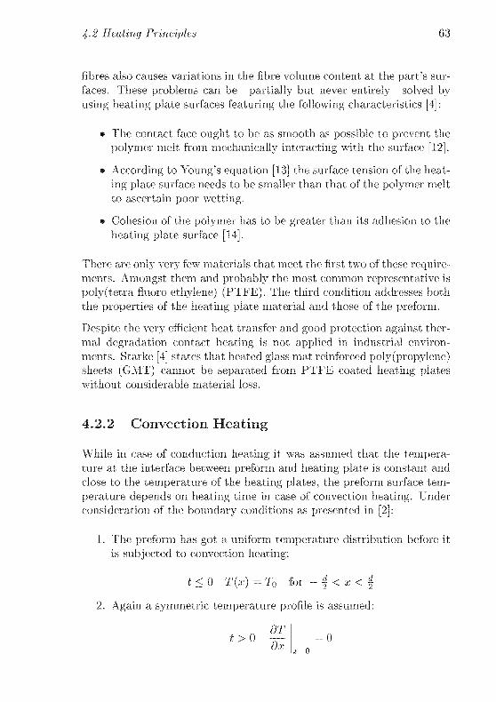
4-2 Heating Principles 63
fibres also causes variations in the fibre volume content at the part's sur¬
faces. These problems can be partially but never entirely solved by
using heating plate surfaces featuring the following characteristics [4]:
» The contact face ought to be as smooth as possible to prevent the
polymer melt from mechanically interacting with the surface [12].
* According to Young's equation [13] the surface tension of the beat¬
ing plate surface needs to be smaller than that of the polymer melt
to ascertain poor wetting.
• Cohesion of the polymer has to be greater than its adhesion to the
heating plate surface [14].
There are only very few materials that meet the first two of these require¬
ments. Amongst them and probably the most common representative is
poly(tetra fluoro ethylene) (PTFE). The third condition addresses both
the properties of the heating plate material and those of the preform.
Despite the very efficient heat transfer and good protection against ther¬
mal degradation contact heating is not applied in industrial environ¬
ments. Starke [4] states that heated glass mat reinforced poly(propylene)sheets (GMT) cannot be separated from PTFE coated heating plateswithout considerable material loss.
4.2.2 Convection Heating
While in case of conduction heating it was assumed that the tempera¬
ture at the interface between preform and heating plate is constant and
close to the temperature of the heating plates, the preform surface tem¬
perature depends on heating time in case of convection heating. Under
consideration of the boundary conditions as presented in [2]:
1. The preform has got a uniform temperature distribution before it
is subjected to convection heating:
t < 0 T(x) = To for - f < x < f
2. Again a symmetric temperature profile is assumed:

64 Heating of Fabric Plies
3. Due to the condition of balanced energy flow the preform's surface
temperature is:
dT
M-f-a (7b - Tu
where a is the heat transition coefficient, îj, is the surface temper¬
ature and Tcom is the temperature of the surrounding convertive
media (usually this will be air or rarely N2).2
4. For infinite beating times the preform temperature equilibrates to:
lim T(x) = Ttonvt —too
the heat transfer equation can be solved as described by [10]. The surface
temperature 7|, is obtained as:
Tb - T0 ^ 2Bi / 24aA
W^ =l-£ Bi(Bi + l)+<6XP (-"»-rfTj (4-)
with the Biot-number defined as Bi =jj
and un being the nth solution
of the transcendent equation u tan u = Bi.
The temperature at the preform's midplane T\i is given as:
( 24«A
ï'conv ïb ^ Bi (Bi + 1) + nl cos u„K '
And finally the average preform temperature (T) is:
(T)-To ^ 2Bi2 / 24aA
-* rnnv * 0
Brinken [2] found that using only the first addend delivers results within
a 10 % error margin if Fo • Bi > 5.
Determination of the heat transfer coefficient a is problematic. In case
of free convection its value ranges from 3 to 20 W m~2 K whereas for
2 The problem of polymer degradation might be solved at least partially by employ¬
ing inert gas atmosphere, but such a system required to be hermetically encapsulated.This would drastically increase the costs of the heating equipment and therefore such
a heating system is only imaginable on a laboratory scale.

4-2 Heating Principles 65
forced convection it is 10 to 100 Wm 2K [2]. Henceforth a is assumed
to equal 15 Wm2 K.
It is obvious according to the third boundary condition that heat can
only be transferred to the preform as long as Tt.onv > Tb. This also
implies that there is no risk of overheating and thus degrading the pre¬
form if the temperature of the convective media is lower than a critical
temperature Tcr;t at which the preform polymer begins to suffer from
oxidative degradation. In practice, however, Tronv is usually higher than
Terit to accelerate the heating process. This represents a compromisebetween as short as possible heating time and processing safety.
Convection heating is successfully applied for unconsolidated (porous)
preforms whereas the small heat transfer coefficient a depicts a serious
drawback if it is desired to heat consolidated preforms by using this
heating principle.
4.2.3 Heating by Interaction with Electro-MagneticFields
In contrast to conduction and convection heating, where the heat is
transported through a heat conducting medium, energy transfer by
electro-magnetic interaction is also possible in vacuo. In principle, any
kind of radiation can transfer energy to any kind of matter, as long as the
considered matter at least partially interacts with the electro-magneticfield emitted by the heater; i.e. part of this field has to be absorbed bythe preform.
An interesting heating approach is exemplified by the use of oscillatory
magnetic fields to induce eddy currents in an electrically conductive ma¬
terial. A laboratory pultrusion apparatus for production of carbon fibre
reinforced plastic rod like structures using an induction coil for heating-was designed by Rajaiah et al. [15] in 1984, and a number of more recent
publications demonstrates the current interest in this method [16 19].
However, amongst the methods using electro-magnetic fields to heat
the preform, heating by thermal radiation—in fact infra-red radiation—
is most common and successfully applied for heating of consolidated
composite sheets in industrial environments [8]. Some efforts were taken
to numerically model preform heating by infra red radiation absorptionof consolidated composite sheets [20, 21]. For present purposes it will
suffice to consider the analytical solution of the heat transfer equation.

66 Heating of Fabric Plies
The boundary conditions for two sided infra red radiation heating are
[2, 3]:
1. Homogeneous temperature over the thickness of the preform can
be assumed before it is subjected to heating:
t < 0 T(x) = T0 for - f < x < f
2. As two sided heating is considered, a symmetric temperature pro¬
file is assumed:
r
dTt>0
to= 0
x-0
3. The heat flow qo transmitted into the preform over its surfaces is
constant:
n ,dT
t > 0 q0 = -A —
dx
4. Heat loss due to convection to the environment is neglected:
t>{) a(T-T0)\. d=0\x -2
According to [10] the preform temperature is:
/6,2d'2
l — Jopcpd 2A I 3d2
2 ^ (-1)" (2mrx\ ( 9 94ai
(4.8)
n-l
Equation 4.8 allows for determining the temperature profile over the
whole cross section of the preform. Only two areas arc of technical
interest though:
1. the surface temperature Tb because there the highest temperatures
have to be expected and the surface is thus most susceptible for
material damage due to overheating; and
2. the midplane temperature Tm because it determines the required
heating time to achieve processing temperature.

4-2 Heating Principles 67
Equation 4.8 therefore simplifies to:
2A(7'b-7o) Aat 1 2 ^ (-1)"r-i w
=t- — > — cos «TT
<7o« « 3 rA z—j n2
n ?4ar.
exp | -71-7T-^
(4.9)
and
2A (TM - Tp) 4a* 1 2^(-l)" / 224aAOO
(4.11)
cjod cP 6 7T2 ^—' n2 \ d'2
for the surface and the midplane temperature, respectively. In [2] it
is shown that the sum converges to null for Fo > 0.8. For practicalestimations of the temperature evolution at the preform's surface and
midplane. Equations (4.9 and 4.10) can therefore be further simplifiedto:
2A (7'b - Tp)___
1 4at
^orf~
?>+lF
and
2A (7m - T0)_
Aat 1
qod~~
cP 3{ }
One of the problems of the analytical solution is the necessity of knowingthe net heat flow qo that passes through the preform surfaces. Partic¬
ularly the convective loss is difficult to quantify. If reliable data of the
surface temperature after an arbitrary time of heating exist, the heat
flow can be determined by solving Equation4.9 for qo.
Infra red radiation combines the advantage of contact free heating and
relatively short heating time. The penetration depth of infra red radi¬
ation is on the order of a few 10"~6 m. Due to the small penetration
depth absorption of infra-red radiation is restricted to the preform sur¬
face, yielding large temperature gradients over the preform cross section.
This is particularly problematic if it is desired to heat thick sheets or ma¬
terials with low thermal conductivity. Due to the very low conductivityof air the latter applies for porous media such as uiiimprcgnated com¬
mingled yarn preforms. If like in the present work infra red heatingis employed to heat unconsolidated composite textiles, the thermal gra¬
dient might even be prohibitively high, so that the surface temperature
is already well above process safety temperature whereas the midplane
temperature is still too low for thermoforming [22].
68 Heating of Fabric Plies
4.2.4 Conversion of Direct Current to Heat
If the considered preform is electrically conductive it is imaginable to
subject such a preform to direct current, which is converted to heat due
to the ohmic drop. Joseph and Viney [23] used this principle to cure
carbon fibre/epoxy composites and showed that the overall energy con¬
sumption is less than | of that necessary for oven curing. Heat transfer
due to electrical current has been extensively investigated during the last
1 | decades and a number of publications issuing this strategy has been
presented by several authors [24-37]. All of these publications deal with
the welding of reinforced thermoplastics using an electric current to heat
the weld joint area.
A complete production method for carbon fibre reinforced thermoplas¬tics made from Schappe Techniques carbon/PA-12 commingled yarn
incorporating electric current as a heat source to heat the preform to
thcrmoforming temperature has been developed by RocTool.3 But—
to the best knowledge of the present work's author—no scientific article
issuing resistance heating of textile preforms prior to thcrmoforming has
been published to date.
Due to material inhomogeneitics (e.g. broken fibres if continuous fibre
reinforcement is considered and/or local variations of the fibre fraction)large thermal gradients over the thickness, length and width of the pre¬
form can develop during heating. Continuous fibre reinforced preformsare expected to be heated less homogeneous than textile preforms with
discontinuous fibre reinforcement since points of irregular material prop¬
erties are rare in the former whereas in case of the latter such points are
regularly distributed and exhibit extremely high density in the whole
stack of fibre material. A small number of inhomogeneities cause large
gradients in the electric field due to extreme variations of local electric
resistivity. In case of regular distribution of defects on a microscopicscale the material appears to have a homogeneous overall resistivity.
If no other effects but temperature increase due to the electrical power
input were considered, the preform temperature would increase linearlywith heating time. Heat loss as a result of convection and conduction,
where in the preform generated heat is transferred to the immediate
environment, has to be accounted for to predict the preform temperature
as a function of beating time.
A transient three-dimensional finite clement heat transfer model for rc-
3RocTool, BP 341 Savoie Technolac, 73375 Le Bourget du Lac Cedex, France
4-3 Experimental 69
sistance welding has been presented by Ageorges et al [33]. It can be
expected that this model is also valid for the heating of unconsolidated
commingled yarn preforms as they are employed throughout this work.
However, the present study on resistance heating is purely experimen¬tal and thus modelling of the evolution of temperature as a function of
heating time and preform coordinates is not performed here.
4.3 Experimental
Heat transfer according to some of the above discussed heating princi¬
ples were also investigated on an empirical level. Experimental set-ups
and procedures for the empirical study of heating principles for uncon¬
solidated commingled yarn fabric ply stacks are sketched in this section.
4.3.1 Conduction Heating
For contact heating experiments four plies of woven fabric of commin¬
gled carbon/PA 12 fibre yarn at 64 weight % carbon fibres were put
between PTFE-coatcd press plates mounted on a hydraulic hot press.
The temperature and closing pressure were set to ~240 °C and 6-10° Pa,
respectively.The temperature was recorded by means of five J-type ther¬
mocouples positioned randomly between the 2nd and the 3rd ply (i.e. at
the midplane only) and the temperature readings of these were averaged.
4.3.2 Infra-Red/Convectioe Heating
Temperature evolution during infra-red heating was studied by subject¬
ing again stacks of four plies of woven commingled yarn fabrics to the
electro-magnetic field of infra-red radiators. Square preform cuts of
40 cm width were used. The fabric stacks were clamped into an alu¬
minium blank holder on all four sides. An infra-red heating device with
48 radiators of 1 kW maximum electrical power intake each for both
upper and lower radiation field, resulting in a total electrical power of
96 kW was used. The two radiation fields were adjustable to the desired
distance between radiator and sample laminate surface. Temperatures
were recorded by means of J type thermocouples at 0.5. 2.5, 6.5, and
17 cm distance from the clamps of the blank holder and at the interface
70 Heating of Fabric Plies
of each two neighbouring fabric plies. Radiation intensity was electroni¬
cally controlled by maintaining the radiator glass tubes' surface temper¬
ature constant. For this purpose each radiator unit was equipped with
a thermocouple.
4.3.3 Direct Current Heating
A single commingled yarn fabric ply of 12 cm width and 26 cm lengthwas subjected to resistance heating. The fabric was placed between
thermally insulating Pyrotek plates and slightly pressurised (1200 Pa).The current loop was closed with bulky copper electrodes of the same
length as the width of the fabric ply. The experimental set up also
showing the thermocouple positions is depicted in Figure 4.1.
4.4 Results and Discussion
Experimental results together with respective analytical solutions of con¬
duction, convection/infra-red, and electric resistance heating are sum¬
marised in Figures 4.2, 4.5, and 4.6. Figure 4.4 provides experimentaldata of the combined infra red and convection heating experiments vi¬
sualised as function of heating time and distance from blank holder
clamps. The so resulting surface plot shows the temperature evolution
at the midplane of the fabric ply stack and at different distances from
the clamps (solid lines). Temperatures between the measured values
were non-linearly interpolated. It is obvious from Figure 4.4 that the
influence of a heat conductive blank holder is only relevant up to ap¬
proximately 20 mm distance from the clamp. From a technical pointof view this is an important value to determine the initial size of fabric
cuts for a given part and, therefore, to estimate the waste material. In
case of infra red/convection and electrical resistance heating experimen¬tal results are given as scatter bands representing the 95 % confidence
interval of the Student T-distribution around the average value.
For each investigated heating method an empirical parameter study was
performed to obtain close to optimal heating parameters in terms of ho¬
mogeneous temperature distribution and short heating time. Figures 4.2
to 4.6 represent experimental results as obtained at optimised heating
parameters, which are given in Table 4.1. The analytical solution as
given in Equation (4.3) agrees relatively well with the experimental con-

4-4 Results and Discussion 71
iPyrotck Plate
Electrode
Pyrotek Plate *> Fabric
T
Upright
projection
Horizontal
projection
Figure 4.1: Schematic illustration of the experimental set-up for resistance
heating
tact heating data if 4 addends of the sum are taken into account. Fig¬ure 4.3 shows the temperature as plotted versus the 7"o«r«er-Number
on a logarithmic scale for different values of n. For the time resolution
of present interest using only 2 addends would actually already deliver
sufficiently accurate results. However, with these day's computing ca¬
pacities it makes no real difference if the sum is abbreviated already after
the first addend or after the tenth. In other words, it does not hurt to
take a few more addends into account even if the improved accuracy is

72 Heating of Fabric Plies
250
20 30
Time [si
50
Figure 4.2: Conduction heating results as compared with analytical solution
according to Equation (f-3) with n = 4.
not needed. Here, 4 addends are used for all calculations.
As visible in Figure 4.5 the analytical solution for pure infra-red heat¬
ing massively overestimates the preform temperature whereas convection
heating underestimates it. At the here employed low radiator tempera¬
ture it is therefore self evident to assume a combination of heating due
to radiation absorption at the preform surface and hot air convection,where the hot radiators transfer heat to the surrounding air. Radiation
absorption is only initially predominant. With increasing air temper¬
ature convection becomes the driver for further preform heating and
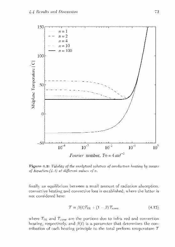
4 4 Results and Discussion 73
Fourier number, Fo = 4 atd
Figure 4.3: Validity of the analytical solution of conduction heating by means
of Equation (4 3) at different values of n
finally an equilibrium between a small amount of radiation absorption,convective beating and convective loss is established, where the latter is
not considered here:
T = 3(t)Tm + (1 - 3) 7'C( (4.13)
wheie T\fi and Tconv are the portions due to infra led and convection
heating, respectively, and 3(t) is a paiameter that determines the con¬
tribution of each heating principle to the total preform temperature T
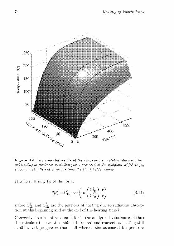
74 Heating of Fabric Plies
250.
- 2004U
3 150.
E
ß 100.
SO-
150
A
%*%>
100 600
^,-^^
50400
%,200
X0 0
f&ieV*
Figure 4.4: Experimental results of the temperature evolution during infrared heating at moderate radiation power recorded at the midplane of fabric plystack and at different positions from the blank holder clamp.
at time t. It may be of the form:
3(t) = C°IR PXP (4.14)
where C°R and CfR are the portions of heating due to radiation absorp¬tion at the beginning and at the end of the heating time f.
Convective loss is not accounted for in the analytical solutions and thus
the calculated curve of combined infra red and convection heating still
exhibits a slope greater than null whereas the measured temperature

4-4 Results and Discussion 75
stays constant after some time. Note that no experimental temperature
data of the preform surfaces were recorded. This is most probably the
reason for the somewhat higher surface temperature prediction of the
combined infra red/convection model as compared with the experimen¬tal results.
Resistance heating results imply a simple square root relationship be-
0 100 200 300 400 500 600 700
Time [si
Figure 4.5: Experimental results of the temperature evolution during infrared heating at moderate radiation power Experimental values are comparedwith analytical solutions according to Equation? (4 5. 4-6< 4 9> and 4 10) with
n = 4

76 Heating of Fabric Plies
tween preform temperature and time:
T = T0 + byrt (4.15)
where Tq is the preform temperature before circuit closure and h is a con¬
stant that depends on current density I, voltage U, i.e. on power input
per preform volume V = III, and heating conditions such as presence
or absence of pressure PA and theimal insulation. For the above pre¬
sented set up and beating parameters as given in Table 4.1 one obtains
6 = 19.5.
250
200
P 150
£ 100
Figure 4.6: Erpeiirnental results of the temperature evolution during eleetriial
resistance heating and corresponding square root fit to the ecperimental data
as given m Equation (4 15)
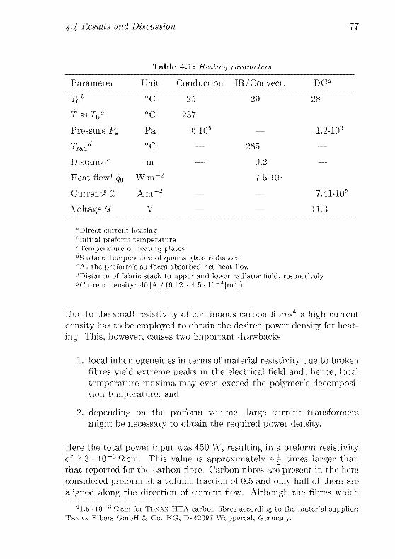
4-4 Results and Discussion 77
Tabic 4.1: Heating parameters
Parameter Unit Conduction TR/Convect. DCa
ry b °C 25 29 28
f « IV °c 237 — —
Pressure PA Pa 6-105 — 1.2-103
TIildd °C 285
Distance^ m 0.2
Heat flow-' qo Wm~2 7.5-103
Current3 I Am2 7.41-105
Voltage U V — — 11.3
"Direct cuirent heating^Initial preform temperatun3
^temperature of heating plates''Surface Temperature of quartz glass radiators
"At the preform's surfaces absorbed net heat flow
'Distance of fabric stack to upper and lower radiator field, respectiveh«Current density: 40 [A/ (0.12 - 4.5 i04[m2])
Due to the small resistivity of continuous carbon fibres4 a high current
density has to be employed to obtain the desired power density for heat¬
ing. This, however, causes two important drawbacks:
1. local inhomogeneities in terms of material resistivity due to broken
fibres yield extreme peaks in the electrical field and, hence, local
temperature maxima may even exceed the polvmer's decomposi¬tion temperature: and
2. depending on the preform volume, large current transformers
might be necessary to obtain the required power density.
Here the total power input was 450 W. resulting in a preform resistivityof 7.3 • 10~3Ocm. This value is approximately 4^ times larger than
that reported for the carbon fibre. Carbon fibres arc present in the here
considered preform at a volume fraction of 0.5 and only half of them are
aligned along the direction of current flow. Although the fibres which
41.6 -10 3 f2cm foi Tknax HT4 carbon fibres according to the material supplier:Te\ax Fibers GmbH k Co. KG, D 42097 Wuppertal. Germany.

78 Heating of Fabric Plies
are aligned transverse to the current flow serve as current bridges theyincrease the prefoim's icsistivity compaied to unidirectional fibre orien¬
tation. The actual conductive preform cross section is only somewhat
laigei thanj
of the macroscopic preform cross section. The resistivityof textile preforms made from discontinuous aligned carbon fibres is thus
only slightly smallei than that of continuous carbon fibre preforms. But
due to the very large number of current brakes and re-routingh from
one fibre to its aligned and non-aligned neighbours homogeneous heat¬
ing is achieved nevertheless. The problem of the required high current
densities, however, remains.
References
[1] U. P. Breuer. Beitrag zur Umformtechnik gewebeverstärkter Ther¬
moplaste. In Fortschritt-Beneide VÜI, number 433 in Reihe 2: Fer¬
tigungstechnik. \TJI Verlag, Düsseldorf, 1997.
[2] F. Brinken. Untersuchungen zur Wärmeübertragung beim Thermo-
forrnen von Thermoplasten. PhD thesis, RWTH Aachen, 1979.
[3] S. Delaloye. Die Diaphragma Technik, ein Anlagenkonzept zur
automatisierten Fertigung kontinuierlich faserverstärkter Thermo-
plastbauteile. PhD thesis, Swiss Federal Institute of Technology,Zurich, Switzerland. 1995. Diss. ETII No. 11151.
[4] J. Starke. Beiträge zum Pressen langfaserverstärkter Kunststoffe.Number 21 in Aachener Beiträge zur Kunststoffverarbeitung. Verlagder Augustinus Buchhandlung. Aachen, 1997.
[5] Anonymous. GAIT frontend for the VW Golf. Reinforced Plastics,
pages" 43-45. 1992.
[6] M. Mahlke. G. Menges. and G. Michaeli. New strategies to pre¬
heat glass-mat reinforced thermoplastics (GMT). ANTEC89, pages
873 875, 1989.
[7] K. O'Brien and S. Kasturi. A computational analysis of the heatingof glass-mat thermoplastic (gint) sheets by dual beam microwave
sources. Polymer Composites, 15:231-239, 1994.
[8] M. D. Wakeman, T. A. Cain, C. D. Rudd, R. Brooks, and A. C.
Long. Compression moulding of glass and polypropylene composites
4-4 References 79
for optimised macro and micro mechanical properties 1 commin¬
gled glass and polypropylene. Composites Science and Technology,58:1879 1898. 1998.
[9] II. Tautz. Wärmeleitung und Temperaturausgleich. Verlag Chemie.
Weinheim, 1971.
[10] II. S. Carslaw and J. C. Jaeger. Conduction of Heat in Solids.
Oxford at the Clarendon Press, 2nd edition, 1959.
[11] G. Wübken. Einfluss der Verarbeitungsbedingungen auf die inne¬
re Struktur thermoplastischer Spritzgussteile unter besonderer Be¬
rücksichtigung der Abkühlverhältnisse. PhD thesis, RWTH Aachen,1974.
[12] C. Bischof and W. Possart. Adhäsion, theoretische und experimen¬telle Grundlagen. Berlin. 1982.
[13] P. Young. Cohesion of fluids. Transactions of the Royal Society of
London, 95:65, 1805.
[14] L. II. Sharpe and II. Schornhorn. Advances in Chemistry. 43. Wash¬
ington D.C., 1964.
[15] K. Rajaiah, N. Ramaswamy, N. K. Naik, V. P. S. Singh. S. Surya-
narayan, and C. P. Jain. Design and development of pultrusion
process with induction and dielectric heating for frp composite man¬
ufacture. Transactions of the Indian Institute of Metals, 37(2):116,1984.
[16] W. Lin and O. Buncman. Induction heating model for graphite
fiber/thermoplastic matrix composites. SAMPE Journal. 27(6) :45-
51, 1991.
[17] L. Augh and J.W. Gillespie, Jr. Degradation of continuous car¬
bon fiber reinforced polyetherimide composites during induction
heating. Journal of Thermoplastic Composite Materials, 14:96 115.
2001.
[18] S. Yarlagadda, II.J. Kim, and J.W. Gillespie. Jr. A study on the
induction heating of conductive fiber reinforced composites. Journal
of Composite Materials. 36(4):401 421. 2002.
80 Heating of Fabru Plies
[19] II.J. Kim. S. Yarlagadda, J.W. Gillespie, Jr.. N.B. Shevchenko, and
B.K. Fink. A study on the induction heating of carbon fiber rein¬
forced thermoplastic composites. Journal of Advanced Composite
Materials, 11(1)-71 80,2002
[20] G J. Sweeney, P. F. Monaghan, M. T. Biogan, and S. F. Cassidy.Reduction of infrared heating cycle time in processing of thermo¬
plastic composites using computer modeling. Composites Manufac¬
turing, 6(3-4) :255-262. 1995.
[21] J. E. Cunningham. P. F. Monaghan, and M. T. Biogan. Predic¬
tions of the temperature profile within composite sheets during pre¬
heating. Composites Part A, 29A:51-61. 1997.
[22] C. Enge. Mechanische Eigenschaften von schnell konsolidiertem Hv-
biidgairihaibzeug. Semesteiarbeit. Institut für mechanische Sys¬
teme, EIH Zürich, 2000.
[23] C. Joseph and C. Viney. Electrical îesistance curing of caibon-
fibre/epoxv composites. Composites Science and Technology,60:315-319. 2000.
[24] E. C. Eveno and J W. Gillespie, Ji Resistance welding of giaphite
polyetheretherketone composites: An experimental investigation.Journal of Thermoplastic Composite Materials, 1:322-338. 1988.
[25] T. B. Jakobsen. K. C Don, and J. W. Gillespie, Jr. Iwo-
dimensional thermal analysis of resistance welded theimoplastic
composites. Polymer Engineering and Science, 29:1722 1729, 1989.
[26] R C Don, L. Bastien, I. B. Jakobsen, and J. W. Gillespie, Ji
Fusion bonding of thermoplastic composites by resistance heating.SAMPE Journal. 26(1).59 66, 1990.
[27] C. L. Lambing, R. C. Don, S. M. Andersen, S. T. Holmes. B. S.
Leacb, and J. W. Gillespie, Jr. Design and manufactuie of fan auto¬
mated resistance welder foi theimoplastic composites. ANTEC'91,
pages 2527 2531. 1991.
[28] R. C. Don, J. W. Gillespie. Jr.. and C. L. T. Lambing. Experimentalcharacterization of pi ocessing pei formance relationship of resitance
wlded graphite/poletberethei ketone composite joints. Polymer En¬
gineering and Science, 32:621 631. 1992.

4-4 References 81
[29] X. R. Xiao, S. V. Iloa, and K. N. Steet. Processing and modellingof resistance welding of ape 2 composite. Journal of Composite
Materials, 26:1031 1049, 1992.
[30] S. T. Holmes and J. W. Gillespie, Jr. Thermal analysis for resistance
welding of large-scale thermoplastic composite joints. Journal of
Reinforced Plastic and Composites. 12:723 736, 1993.
[31] I. Howie, J. W. Gillespie, Jr., and J. Smiley. Resistance weldingof graphite-polyarylsulfoiie/polysulfonc dual-polymer composites.
Journal of Thermoplastic Composite Materials, 6:205-225, 1993.
[32] M. Arias and G. Ziegmann. The impulse resistance welding: a new
technique for joining advanced thermoplastic composite parts. In
41st International SAMPE Symposium., pages 1361 1371, 1996.
[33] C. Ageorges, L. Ye, Y.-W. Mai, and M. Hon. Characterisation
of resistance welding of lap shear coupons, part i: Heat tranasfer.
Composites Part A, 29:899 909, 1998.
[34] C. Ageorges, L. Ye, Y.-W. Alai, and AL Hon. Characterisation
of resistance welding of lap shear coupons, part ii: Consolidation.
Composites Part, A, 29:911-919, 1998.
[35] C. Ageorges, L. Ye, Y.-W. Alai, and M. Hou. Characterisation
of resistance welding of lap shear coupons, part iii: Crystallinity.
Composites Part A, 29:921 932, 1998.
[36] C. Ageorges, L. Ye. and M. Hou. Experimental investigation of
the resistance welding for thermoplastic matrix composites, part i:
heating element and heat transfer. Composites Science and Tech¬
nology, 60:1027 1039, 2000.
[37] C. Ageorges, L. Ye. and M. Hou. Experimental investigation of the
resistance welding for thermoplastic matrix composites, part ii: op¬
timum processing window and mechanical performance. CompositesScience and Technology, 60:1191-1202, 2000.

82 Heating of Fabric Plies
Chapter 5
Laminate Quality of
Stamp Formed
Commingled Yarns
5.1 Introduction
Owing to commingled yarns with very high degrees of intermingling be¬
ing unavailable until recently, the existing product forms w7ere chiefly em¬
ployed in combination with the compression moulding process [1-5]. In
case of compression moulding, already relatively inhomogeneous blended
yarns deliver laminates of high quality. But the degree of comminglingis identified to affect the mechanical properties of the consolidated lam¬
inate [2, 3]. Commingled yarns of exceptional blending quality emerged
only recently, partially as a result of preliminary results of this work
taking influence on the material supplier's preform development .
For the purpose of this study, two newly developed commingled yarns
were at the author's disposal, to re-investigate the use of commingled
yarns with the stamp forming process without performing any pre
consolidation intermediate step. In this chapter the sensitivity of the
laminate quality of stamp formed carbon-fibre/poly(laurolactam) (desig¬nated as PA thereafter) and carbon fibre/poly(butylene-terepbthalate)(designated as PBT hereafter) commingled yarns to the variation of yarn
84 Laminate Quality of Stamp Formed Commingled Yarns
structure and processing conditions is investigated. The laminate qual¬
ity is evaluated by means of static mechanical properties of laminates
with unidirectional fibre orientation, void content measurement, and op¬
tical microscopy. The achieved mechanical properties of stamp formed
laminates are compared with those of compression moulded reference
laminates. It is tried to find qualitative relationships between laminate
quality, yarn characteristics and processing conditions mainly on an em¬
pirical level.
5.2 Experimental
This chapter focuses on the empirical investigation of the relationshipbetween yarn architecture, processing parameters and laminate qualityin terms of mechanical properties and void content. Experimental pro¬
cedures to obtain such data are described within this section.
5.2.1 Commingled Yarns and their Characterisation
Three different commingled yarn types as obtained by Schaffe Tecii-
mquks were employed to produce laminates with unidirectional rein¬
forcement fibre orientation. All three yarn types are spun from stretch
broken high tenacity carbon fibres provided by Tenax® and polymer
fibres, resulting in a reinforcement fibre content by volume in the thor¬
oughly consolidated state as noted in Table 5.1. Two of the investigated
yarn types have PA-12 fibres blended with carbon fibres of different
length distribution, and the third yarn type is commingled from carbon
fibres of a standard length distribution and PBT fibres. An overview of
the yarn parameters along with stamp forming processing conditions for
the various laminates is given in Table 5.1. Top view of the standard
grade yarn and cross section of all three yarn types are illustrated in
Figure 5.1 and Figure 5.2 5.4, respectively. The two polymer filament
bundles crosswise helically surrounding the yarn as visible in Figure 5.1
grant the yarn a certain strength necessary for further textile treatment
such as weaving or braiding. The main part of polymer fibres, however,is also aligned parallel to the yarn axis and is contained within the yarn
with outstanding degree of mingling as visible in Figure 5.2-5.4. The
mingling quality depends on:
1. the reinforcement fibre volume fraction,
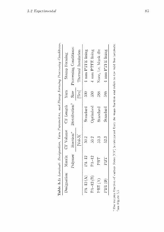
Table
5.1:Laminate
Designation,
YarnParameters,
andStampForming
Processing
Conditions
Designation
Matrix
CFVolume
Polymer
Fraction'1
[Vol-%]
PA-12(A
)PA-12
50.2
PA-12(B
)PA-12
50.2
PBT
(A)
PBT
52.3
PBT
(B)
PBT
52.3
CF
Length
Yarn
StampForming
'istribution6
Size
ProcessingConditions:
[Tex]
Thermal
Insulation
Standard
500
4mmPTFE
lining
Optimised
500
1mmPTFE
lining
Standard
588
None,
i.e.
blank
die
Standard
588
4mmPTFE
lining
"Thevolume
fractionofcarbon
fibres(CF)
iscalculatedfromthemass
fractionand
referstothevoid
freelaminate.
6see
Figure
5.5

86 Laminate Quality of Stamp Formed Commingled Yarns
Figure 5.1: Micrograph of standard grade commingled yarn (top view)
2. the fibre length distribution of reinforcement and polymer fibres,
3. the yarn size [6], and
4. the ratio of reinforcement to polymer fibre diameters [7. 8].
Increasing number of fibres to be blended complicates the commingling
process and results in less intimate blending quality. Already a small
number of very long fibres affects the blending quality disadvantageously,
and, finally, similar fibre diameters of the blended fibre types stronglv
support good mingling quality. As the carbon fibres are stretch broken
from continuous filaments the fibre length distribution is not adjustablearbitrarily. The cumulated relative fibre numbers as a function of fibre
length for all fibre types discussed here are given in Figure 5.5. The fibie
numbers were calculated from measured mass fractions for each class of
fibre lengths 4-i < t < U- The cumulated relative fibre number n at

5.2 Experimental 87
Figure 5.2: Micrograph of unconsolidated commingled yarn cross section:
standard grade (PA 12 (A)).
length class f, can be expressed as:
n(A) = V (5.1)
?n—i
where N(fm) is the observed number of fibres at length class £m,i = 1.2,...,/; is the number of the considered length class and k is
the number of the length class, which contains the longest fibres. As
visible in Figure 5.5, adjusting the stretch braking process to deliver
carbon fibres of a limited length matching the maximum length of the
polymer fibres shifts the whole fibre length distribution towards shorter
fibres. The average fibre length is 35.1 and 22.3 mm for standard and
shortened carbon fibres, respectively, i.e 50 % of the standard fibres are
between 10 and 35.1 mm long whereas 50 % of the shortened fibres ex¬
hibit lengths between 10 and 22.3 mm. The smaller yarn size and the
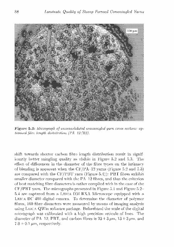
88 Laminate Quality of Stamp Formed Commingled Yarns
Figure 5.3: Micrograph of unconsolidated commingled yarn cross section: op¬
timised fibre length distribution (PA 12(B)).
shift towards shorter carbon fibre length distribution result in signif¬
icantly better mingling quality as visible in Figure 5.2 and 5.3. The
effect of differences in the diameter of the fibre tvpes on the intimacyof blending is apparent when the CF/PA 12 yarns (Figure 5.2 and 5.3)are compared with the CF/PBT yarn (Figure 5.4)): PBT fibres exhibit
smaller diameter compared with the PA-12 fibres, and thus the criterion
of best matching fibre diameters is rather complied with in the case of the
CF/PBT varn. The micrographs presented in Figure 5.1 and Figure 5.2-
5.4 are captured from a Leica DM RXA Microscope equipped with a
Leica DC 480 digital camera. To determine the diameter of polymer
fibres, 100 fibre diameters were measured by means of imaging analysis
using Leica QWin software package. Beforehand the scale of the digital
micrograph was calibrated with a high precision reticule of lines. The
diameter of PA 12, PBT, and carbon fibres is 23 ± 3 pm. 13 ± 3 pm, and
7.0 ± 0.1 pm. respectively.
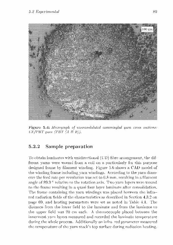
5 2 Experimental 89
Figure 5.4: Micrograph of unconsolidated commingled yarn cross sections
CF/PBT yarn (PBT (A & B))
5.2.2 Sample preparation
To obtain laminates with unidirectional (UD) fibre arrangement, the dif¬
ferent yarns weie wound from a coil on a particularly foi this purpose
designed frame by filament winding. Figure 5.6 shows a CAD model of
the winding fiame including yain windings. According to the yarn diam¬
eter the feed rate per revolution was set to 0.8 mm. ic&ultiiig in a filament
angle of 89.9 ° relative to the rotation axis. Two yam layers weie wound
to the fiame resulting in a quasi four laver laminate aftei consolidation.
The fiame containing the \arn windings was placed between the infra¬
red radiation fields of the cliaiacteiistics a& desciibed in Section 4.3.2 on
page 69. and heating parameters were set as rioted in Table 4.1. The
distance from the lower field to the laminate and from the laminate to
the upper field was 20 cm each. A thermocouple placed between the
innermost vain layers measured and recorded the laminate temperature
during the whole process. Additionally an infra red pyrometer measured
the temperatuie of the yarn stack's top surface during radiation heating.

90 Laminate Quality of Stamp Formed Commingled Yarns
^ 0.8
O
5
Q
0.6
>
1 0.4 hPi
"3
0.2
' '
—e—-CF
—•---CFs
—-A—-PA-12
- -- -PBT
ig ffl f 3 0j ®—i-
_L
50 100 150 200
Fibre Length Class [mm]
250
Figure 5.5: Cumulated relative number of fibres as a function of the fibre
length class CFs corresponds to the shortened caibon fibre length distribution
The yarn stacks were transferred to the hot press as soon as the lam¬
inate's top suiface temperature as measured by the pyrometer reached
220 °C in the case of the CF/PA 12 yarns and270 °C for the CF/PBTyarn, respectively. The press plates' temperature was maintained con¬
stant below the polymer's solidification temperature, namely at 155 °C
for CF/PA 12 and 190 °C for CF/PBT. The die was machined from
aluminium and coated with a 12 pm thick layer of Ni PTFE to support
release of processed laminates.
Since fibre impregnation and solidification of the polymer take place in
a single process step, too fast cooling is prohibitive for good laminate
quality [9, 10]. To extend the time span available for consolidation the
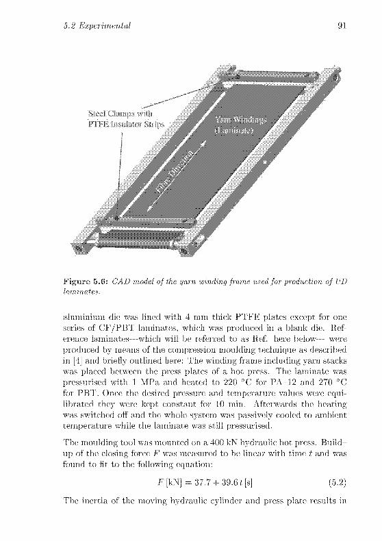
5.2 Experimental 91
Figure 5.6: CAD model of the yarn winding frame used for production of UD
laminates.
aluminium die was lined with 4 mm thick PTFE plates except for one
series of CF/PBT laminates, which was produced in a blank die. Ref¬
erence laminates which will be referred to as Ref. here below were
produced by means of the compression moulding technique as described
in [4] and briefly outlined here: The winding frame including yarn stacks
was placed between the press plates of a hot press. The laminate was
pressurised with 1 MPa and heated to 220 °C for PA-12 and 270 °C
for PBT. Once the desired pressure and temperature values were equi¬librated they were kept constant for 10 min. Afterwards the heatingwas switched off and the whole system was passively cooled to ambient
temperature while the laminate was still pressurised.
The moulding tool was mounted on a 400 kN hydraulic hot press. Build¬
up of the closing force F was measured to be linear with time t and was
found to fit to the following equation:
F[kN] =37.7 + 39.6 f[s] (5.2)
The inertia of the moving hydraulic cylinder and press plate results in

92 Laminate Quality of Stamp Formed Commingled Yarns
an initial closing force of approximately 40 kN. The here below employed
designation for differently piocessed laminates is given in Table 5.1.
5.2.3 Laminate Characterisation
The L'D laminates were cut parallel and perpendicular to the fibre di¬
rection to obtain samples for flexural tests parallel to the fibre diiection
according to the European Standard EN 2562 and specimens for tensile
tests peipendicular to the fibre direction, respectively The samples for
tensile tests peipendiculai to the fibie diiection weie 30 mm wide bv
130 mm length. End tabs of 30 mm width. 25 mm length, and 2 mm
thickness were cut from ±45° glass fibre epoxy resin laminates and at¬
tached to the tensile test specimens with epoxy based adhesive film.
The volume of consolidated laminate specimens was measured in a
Quaxtachrome Ultrap\ CNOMETER 1000 gas pvcnometer using He¬
lium as the pressure medium. 3 pieces of about 2 • 30 • 30mm^ of each
laminate weie weighed to the closest 10-4 g and put together in the
pvcnometer's sample container. Subsequently, one such sample of each
PA-12 laminate was dissolved in formic acid to extract the fibres and
determine the fibre weight fraction. The suggested solvent foi PBT is
a mixture of phenol and tetrachlorethane [11]. Due to the hazardous
nature of these agents the fibre mass fi action of PBT laminates was as¬
sessed in a different way. The laminate samples were put in an oven
and exposed to hot air at 375 °C for 24 h. Beforehand it was verified bymeans of theimogravimetiical analysis that PB I decomposes sufficientlyfast at this temperature if the measurement cell is purged with oxygen.
Along with the laminate specimens one sample container was filled with
Tenax HTA carbon fibres to evaluate the fibre weight lo&s. Given the
densities of fibres and matrix the theoretic laminate density pt can be
calculated as:
PfPm /~0,
Pt = (5.3)P(Wm + pmW{
with pf the fibie density. pm the matrix density. W{ and wm = 1 —Wf the
mass fi actions of fibres and matrix, respectively. The fraction of voids
remaining in the laminate after consolidation, vY, is determined as
Pi
where p is the measured laminate density.

5.3 Results and Discussion 93
5.3 Results and Discussion
The results of flexural properties parallel to the fibre direction and tensile
properties transverse to the fibre direction are illustrated in Figure 5.7
and Figure 5.8, respectively. Additionally, the test results are summa-
PA-12(A)
PA-12 (B)
D PBT (A)
1200~
1000
800
600
400
200
1 Ref. 2 4 6 8
Applied Consolidation Pressure [MPa]
Figure 5.7: Flexural strength along the fibre direction.
rized in Table 5.2. Other than previously reported [10] a slower coolingwith increasing consolidation pressure was not observed here. The tem¬
perature readings during consolidation of each PBT laminate type were
therefore averaged regardless of the applied consolidation pressure. As
the processing conditions were identical for both PA 12 laminate types
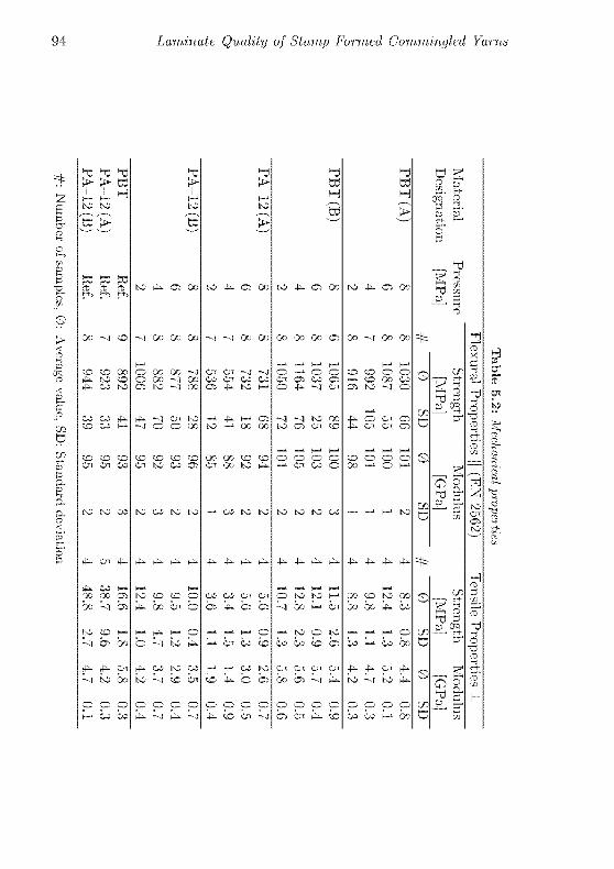
Laminate Quality of Stamp Formed Commingled Yarns
TJ T3 Tl> > Cd
. _H
to to
cd >
33S(D t ^
CD 00
to CO
CO to
co oo 4-CD CO H-
CD CD CO
ci oi co
4* W H
oo oo en
bo ^ on
tO CD l-->
I en oo
4_ 4^ oi
to oo
o o o
— oo co
to 4- en >G0
-J GO GO >G0
O GO GO -JO GO -1 00
CS M S GO
4> ~q On tO
—i o o oo
CD CD CD CD
oi to oo en
to oo to to
4—4-4—4—
to CD CD O
4- GO Ol O
4-
O ~J to »_
4^ CO tO CO
to ~J CD Ol
o o o o
4_ ^J 4- ^1
to 4- en oo
co oi co co
Oi *- M H
— 4- H- O
to — oo oc
GO GO CO CD
Ci 00 to 4-
— co to to
4-4-4-4-
00 CO Oi Ci
en 4— en en
— ^ H-* o
— ci ce o
- H W K)
cd 4- ö en
o o o o
it- b üi m
to 4- en oo
go oo 'Go en
O h- O O
oi en co en
o 4- -r oi
-i -i to œ
to en oi cd
o o o oi—* oi co o
to to to co
4~ 4— 4-- b_
o to to H-»
s bo h bi
h-i to o to
co co co en
Oi Oi Oi Or
bo i» ^t i-
o o o o
en oi 4— co
to 4- en oo
CD co o ot—' co oo co
en to -i o
o oi en
ci oi en
CD O O O
GO h-4 O h-4
4- J_ 4- 4-
OO CD to 00
bo bo 4- ce
^ H-* h-4 O
co i—> co bo
j_ o_ or o-
to ^1 to 4-
o o o o
co ce h-» bo
É2.
<b 2.p IS
c
*
Q
Q
co
Q S"
p t-
*
co
cnj±L t-
0
ST
CT
to
o
3
13
o"d
3-
h-
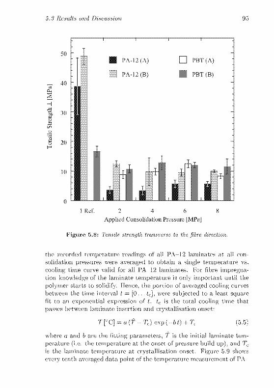
5.3 Results and Discussion 95
PA-12 (A) D PBT (A)
~Z\ PA-12 (B) PBT(B)
1 Ref. 2 4 6 8
Applied Consolidation Pressure [MPa]
Figure 5.8: Tensile strength transverse to the fibre direction.
the recorded temperature readings of all PA-12 laminates at all con¬
solidation pressures were averaged to obtain a single temperature vs.
cooling time curve valid for all PA 12 laminates. For fibre impregna¬tion knowledge of the laminate temperature is only important until the
polymer starts to solidify. Hence, the portion of averaged cooling curves
between the time interval t = [0.. .tc], were subjected to a least square
fit to an exponential expression of t. tc is the total cooling time that
passes between laminate insertion and crystallisation onset:
T [°C] = a (T - Tc) exp (-61) + Tc (5.5)
where a and b are the fitting parameters. T is the initial laminate tem¬
perature (i.e. the temperature at the onset of pressure build up), and Tc
is the laminate temperature at crystallisation onset. Figure 5.9 shows
every tenth averaged data point of the temperature measurement of PA
o
50
40
30
20
10
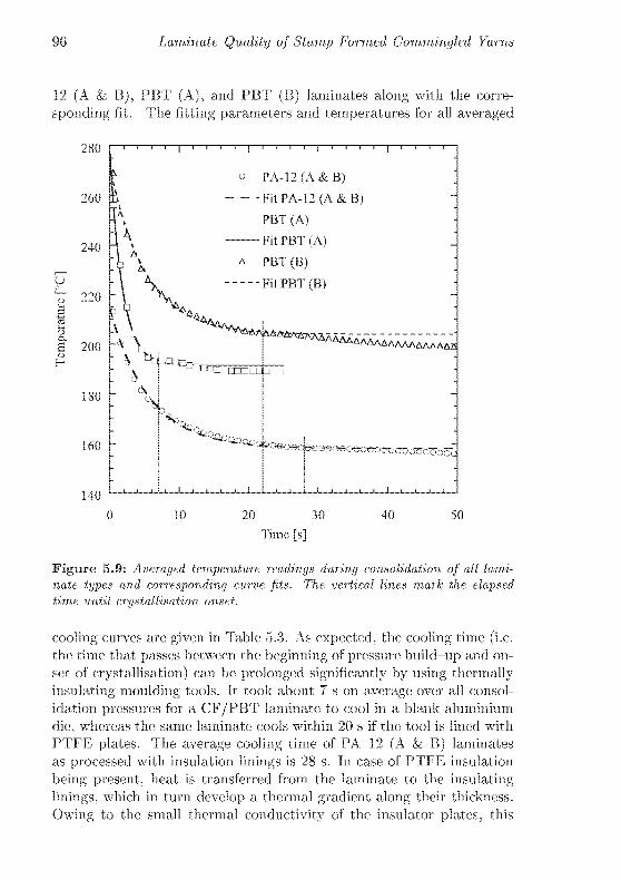
96 Laminate Quality of Stamp Formed Commingled Yarns
12 (A & B). PBT (A), and PBT (B) laminates along with the corre¬
sponding fit. The fitting parameters and temperatures for all averaged
280 i
260
T t 1 1 ! j i 1 1 ! j r-
240
220
140
o PA-12 (A &B)
- -Fit PA-12 (A &B)
PBT (A)
Fit PBT (A)
a PBT (B)
Fit PBT (B)
'^u^jml^,
OwoeoeetseoeoeoTOoooDOüo-C-oöc
J I LJ_J 1 I I 1 1 1 I I 1 ! ! I I 1 ! ! I 1 1 L
10 20 30
Time [s]
40 50
Figure 5.9: Averaged temperature readings during consolidation of all lami¬
nate types and corresponding curve fits. The vertical lines mark the elapsedtime until crystallisation onset.
cooling curves are given in Table 5.3. As expected, the cooling time (i.e.the time that passes between the beginning of pressure build-up and on¬
set of crystallisation) can be prolonged significantly by using thermally
insulating moulding tools. It took about 7 s on average over all consol¬
idation pressures for a CF/PBT laminate to cool in a blank aluminium
die, whereas the same laminate cools within 20 s if the tool is lined with
PTFF plates. The average cooling time of PA 12 (A & B) laminates
as processed with insulation linings is 28 s. In case of PTFE insulation
being present, heat is transferred from the laminate to the insulating
linings, which in turn develop a thermal gradient along their thickness.
Owing to the small thermal conductivity of the insulator plates, this

5.3 Results and Discussion 97
Table 5.3: Parameters of the Cooling Curve Fit
Parameter Unit Laminate Type
PA.
12 (A &B) PBT (A) PBT(B)
f °C 222 273 275
Tc °C 158 192 204
U s 28 7 22
a 0.881 1.07 0. 949
b s1 0.176 0.561 0.193
R2 0.990 0.993 0.994
gradient is flattened slowly, and hence the tool temperature appears to
be set to a higher value as compared with the end temperature of the
laminate processed in the blank tool. This effect will be discussed in
detail in Chapter 6.
Incomplete consolidation severely lowers the mechanical piopeities
transverse to the fibre direction whereas a relatively high residual void
content can be afforded without significant loss of tensile strength alongthe fibre direction. Due to its compressive stress component the bend¬
ing test is more sensitive to variations of impregnation quality than a
standard tensile test along the fibre direction would be. Dry fibres (i.e.fibies that are not supported by matrix) are not capable of withstanding
compressive stresses. The sensitivity of flexural and transverse tensile
strengths on consolidation pressure (Figure 5.7 and Figuie 5.8) show
qualitatiye similarity, which is confirmed by Pearson con elation coeffi¬
cients of 0.99, 0.81, 0.67. and 0.71 for PA-12 .(A), PA-12 (B), PBT (A),PBT (B) laminates, respectively. In the case of transveise strength the
variations with processing pressure are. however, more articulate. This
is attributed to two basic effects, which are schematically illustiated in
Figure 5.10:
1. the void geometry, which is assumed to have an aspect ratio graterthan one with the long axis being parallel to the fibre diiection,and
2. the different crack growth mechanisms in case of longitudinal and
transverse loading.
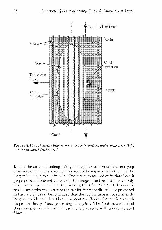
98 Laminate Quality of Stamp Formed Commingled Yarns
Longitudinal Load
Fibres-
Void -
Transverse
Load
Crack
Initiation
/
f
3;
4
Crack
Resin
Crack
f Initiation
"Crack
Figure 5.10: Schematic illustration of crack formation under transverse (left)and longitudinal (right) load.
Due to the assumed oblong void geometry the transverse load carrying-cross sectional area is severely more reduced compared with the area the
longitudinal load takes effect on. Under transverse load an initiated crack
propagates unhindered whereas in the longitudinal case the crack onlyadvances to the next fibre. Considering the PA-12 (A k B) laminates"
tensile strengths transverse to the reinforcing fibre direction as presentedin Figure 5.8, it may be concluded that the cooling time is not sufficiently
long to provide complete fibre impregnation. Hence, the tensile strength
drops drastically if fast processing is applied. The fracture surfaces of
these samples were indeed almost entirely covered with unimpregnatedfibres.
5.3 Results and Discussion 99
The number of dry carbon fibres to be wetted by each molten polymerfibre is predetermined by the fibre volume fraction, the homogeneity of
mingling, and the ratio of carbon to polymer fibre diameter [7]. Hence,
improved blending quality shortens the polymer percolation distance,
and lowers the number of carbon fibres to be wetted by each molten
polymer fibre. The total consolidation time necessary to obtain a void
free laminate strongly depends on the blending quality. The experimen¬
tally validated impregnation model as developed by Bernet ct al. [12]predicts an isothermal impregnation time of little more than 4 min at
220 °C and at consolidation pressures ranging from 10 to 25 bar to ob¬
tain a quasi void free laminate made from CF/PA 12 Schappe Tech¬
niques commingled yarn type with 56 % fibre content by volume. This
commingled yarn exhibits relatively inbomogeneous blending. Bernet et
al. modelled the inhomogeneity by taking reinforcing fibre bundles con¬
taining different numbers of fibres into account. They observed that the
largest carbon fibre bundles comprise between 200 and 250 fibres. The
yarn is assumed to contain two such large fibre bundles and 111 small
fibre bundles of 50 fibres. Considering the micrographs in Figures 5.2-
5.4 it is obvious that the blending is more intimate here than in the
case of the work of Bernet et al. [12], which is attributed to the smaller
fibre volume fraction and enhanced blending technology in the case of
CF/PA 12 yarns, and, additionally, to the smaller polymer fibre diam¬
eter in case of the CF/PBT yarn. The three investigated yarn types
comprise approximately 170, 120, and 50 carbon fibres per large fibre
bundle for PA 12 (A). PA 12 (B), and PBT yarn, respectively. With
yarn and polymer viscosity parameters as noted in Table 5.4 the consoli¬
dation model can now be adapted to the present material characteristics,
using fibre size distribution according to Equation 2.39 with 20 bundle
size classes instead of only two fibre bundle sizes. Generalisation for the
non isothermal case is thereby represented by implementing the viscos¬
ity as a function of temperature [9], which is linked to cooling time via
the fitting function as presented in Equation (5.5). In the present case,
additional difficulties arise due to the fact that the press is not capableof building up the pressure instantaneously upon closing. The time that
passes between tool closing and fully established consolidation pressure
accounts for a considerable portion of the total consolidation time. If
8 MPa are required, it even exceeds the total consolidation time available
for PBT (A) laminates.
Variation of pressure would require a more complex solving methodol¬
ogy of Darcy's equation, since the assumption of constant fibre volume
fraction in the unimpregnated bundle, and thus the fibre velocity being
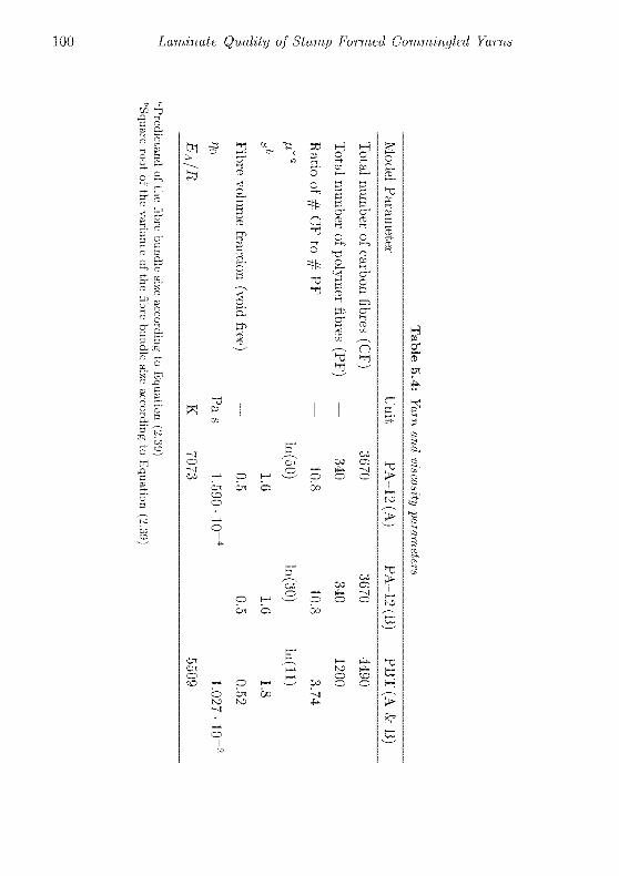
Table
5.4:
Yarnand
viscosityparameters
ModelParameter
Unit
PA
12
(A)PA
12(B)
PBT
(A&
B)
Totalnumber
ofcarbon
fibres(CF)
—
3670
3670
4490
Totalnumber
ofpolymer
fibres(PF)
—
340
310
1200
Ratio
of#CF
to#PF
—
10.8
10.8
3.74
/i*°—
ln(50)ln(30)
ln(ll)
sb1.6
1.6
1.8
Fibrevolume
fraction
(voidfree)
0.5
0.5
0.52
no
Pas
1.590
IQ"4
1.027-IQ"2
EA/R
K7073
5509
"Predictaird
ofthe
fibrebundle
sizeaccording
toEquation
(2.39)'Square
rootofthevariance
ofthe
fibrebundle
sizeaccording
toEquation
(2.39)

5.3 Results and Discussion 101
null, is not correct. Nevertheless the solving methodology suggested by
Bernet et al. [12] was employed here to approximately predict the void
content of stamp formed laminates. At each time increment the appliedconsolidation pressure and its dependant parameters were updated in
accordance with the expression of closing force vs. time as noted in
Equation (5.2) until either the preset maximum pressure was reached
or the consolidation time exhausted, whichever criterion was fulfilled
first. The approximated void contents of each stamp formed laminate
are summarised along with experimental data in Table 5.5. The values
predicted for the PA-12 (A & B) laminates are comparable with those
reported in [9] despite the fact that the authors worked with a less in¬
timate commingled yarn and higher fibre volume content (56 %). They
subjected the yarn stacks to extreme overheating (280 °C) prior to stamp
forming, resulting in much lower initial viscosities and thus faster flow
front advancement. At such high temperatures, however, the polymeris susceptible to degradation and thus the maximum process tempera¬
ture should not exceed 260 °C. The high void content predicted for the
PBT (A) laminates may not surprise as they experienced solidification in
less than 7 s. The influence of consolidation pressure is negligible in the
case of PBT (A) laminates whereas for all the other laminates a slightincrease of void fraction with increasing pressure is calculated. Althoughthe applied pressure is the driving force for flow front advancement it also
influences the permeability of the remaining dry fibre bundles. In the
case of isothermal conditions (i.e.. compression moulding) the consolida¬
tion model suggests the optimum consolidation pressure to be between
1 and 1.5 MPa. The significance of pressure, however, decreases with
increasing processing temperatures. Wakcman et al. [13] also found onlyminor influence of the consolidation pressure on stiffness, strength and
void content, but stated that pressures between 1.5 and 2.0 AlPa are re¬
quired to obtain laminates with low void contents. Compared with the
computed voidage the experimentally obtained values agree only on the
2 MPa level of PA 12 (A) and PA 12 (B) laminates and on the 4 AlPa
level of the PA 12 (A) laminate. This suggests that some of the model
assumptions are not appropriate to the present materials and processingconditions. The model assumes that the fibres are immobile after the
consolidation pressure has been established, and thus fibre flow is not
taken into account. As visible in Figure 5.11 the shape of the original
yarn cross section has altered due to transverse fibre flow.
The yarn flattening caused by transverse fibre flow spreads the fibre
bundles and thus enhances impregnation. Fibre bundle compaction due
to quasi hydrostatic pressure and bundle spreading due to transverse
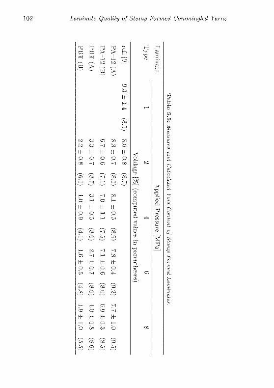
Table
5.5:
Measuredand
Calculated
VoidContent
ofStamp
Formed
Laminates
Laminate
Applied
Piessure[MPa]
T^pe
12
16
8
Yoidage
[%](computedvalues
inpaientheses)
ref.[9]
9.3±
1.4
(8.9)8.0±
0.8
(8.7)
PA
12
(A)8.3±
0.7
(8.6)8.1±
0.5
(8.9)7.8±
0.4
(9.2)7.7±
1.0
(9.5)
PA
12
(B)6.7±
0.6
(7.1)7.0±
1.1
(7.5)7.1±
0.6
(8.0)6.9±
0.3
(8.5)
PBT
(A)3.3±
0.7
(8.7)3.1±0.5
(8.6)2.7±
0.7
(8.6)4.0±
0.8
(8.6)
PBT
(B)2.2±
0.8
(6.0)1.0±0.9
(4.1)1.6±0.5
(4.8)1.9±1.0
(5.5)

5.3 Results and Discussion 103
Figure 5.11: Micrographs of consolidated PBT (B) laminate cross sections:
(a) processed at 2 MPa consolidation pressure.
fibre flow take contradictory effect on fibre impregnation. The former
lowers and the latter increases permeability of the fibre bundle, so that
an optimum pressure exists, at which compaction is least and spreadingmost effective. It was observed for unidirectional laminates of carbon
fibres and poly(ether ether ketone) that transverse fibre flow increases
proportional to the cubic root of the applied pressure [14]. The optimumconsolidation pressure, apparently, depends on reinforcement fibre lengthas well as fibre bundle size and shape, and thus, the optimum consoli¬
dation was different for the various laminate types. This behaviour can
be explained qualitatively by considering the different yarn architectures
and their influence on fibre flow. It was stated that fibre twisting hinders
transverse fibre flow [14]. Fibre locking due to twisting increases with
increasing fibre length, assuming a constant number of fibre crossovers
per fibre unit length. Due to the shorter fibres supporting fibre flow al¬
ready at low pressures, PA 12 (B) laminates exhibit best quality at the
2 MPa level, whereas the PA 12 (A) laminates need to be consolidated
at 6 to 8 MPa to take advantage of fibre flow. In case of the PBT lam-

104 Laminate Quality of Stamp Formed Commingled Yarns
Figure 5.11 (continued): (b) processed at 4 MPa consolidation pressure.
mates, which are spun from stretch broken carbon fibre with standard
fibre length distribution (Figure 5.5), the intimate blending enhances fi¬
bre flow, and thus the optimum laminate quality is achieved at the 4 and
6 AlPa level for PBT (B) and (A), respectively. The difference between
PBT (A) and (B) laminates is attributed to the fast cooling and cor¬
respondingly fast increase of resin viscosity in case of PBT (A), which
calls for higher pressures to induce fibre flow. With regard to the micro¬
graphs in Figure 5.2 the assumption of cylindrical fibre bundles has to
be reconsidered. The fewer fibres a bundle contains the less cylindrically
shaped these bundles tend to be. Oblong bundles arc faster percolated
by the resin as the flow distance is shorter than in case of a cylindricalbundle comprising the same number of fibres. Not only the voidage but
also the size and shape of voids influence the laminate quality in terms
of strength transverse to the fibre direction. Small globular voids, which
are regularly distributed in the laminate, do not affect the transverse
properties significantly as long as the total void fraction is lower than
a critical value. This is reflected by comparison of tensile strength re¬
sults of the different laminate types. Although the PBT (A) laminates

5.3 Results and Discussion 105
Figure 5.11 (continued): (c) processed at 6 MPa consolidation pressure.
exhibit greater void content than the PBT (B) laminates, the transverse
tensile strengths of these laminate types are comparable, particularly at
the 6 MPa consolidation pressure level. This suggests that the effect of
absolute voidagc is overruled by the influence of the size of voids.
The void size can be assumed to decrease with increasing intimacy of
blending, which is experimentally confirmed by comparison of PA 12 (A)laminates with PBT (A) laminates processed at 4 MPa as illustrated in
Figure 5.12 (a) and (b), respectively. The PA-12 (A) laminate (Fig¬ure 5.12 (a)) shows fairly large resin rich areas as well as densely packed
unimpregnated fibre agglomerations, whereas in case of the PBT (A)laminate (Figure 5.12 (b)) a relatively regular distribution of fibres and
matrix with only small fibre agglomerations is observed. The transverse
tensile strength of the compression moulded PBT reference laminate is
much lower compared with the values obtained for the PA 12 laminates.
As mentioned above the CF/PBT yam is a prototype that lacks spe¬
cial fibre conditioning to enhance fibre/matrix adhesion. Furthermore
it was found that PBT is susceptible to degradation if it is exposed

106 Laminate Quality of Stamp Formed Commingled Yarns
Figure 5.11 (continued): (d) processed at 8 MPa consolidation pressure.
to temperatures significantly higher than melting temperature [15]. The
resulting decrease of molecular mass causes embrittlement [16]. Thernio-
gravimetrical analysis of PBT, however, did not reveal any mass loss at
temperatures around 275 °C and exposure times similar to that typicallyused for compression moulding (10 min). On the other hand, decrease of
molecular weight does not necessarily express itself in terms of a generalloss of polymer mass, whereas a decrease of melt viscosity is an indi¬
cator for reduced molecular weight. It was indeed observed, that the
melt viscosity decreased slightly during isothermal viscosimetry, with
the critical exposure time being dependent on the temperature. At 275
C it was found that times of exposure of less than two minutes do not
result in considerable decrease of viscosity, which, in turn, limits the
process safety margin to approximately two minutes of material expo¬
sure to processing temperature. The low transverse tensile strength of
compression moulded PBT laminates is thus attributed to unsatisfactory
fibre/matrix interface and might as well be a result of polymer degra¬dation. In case of stamp formed PBT laminates the total heating time
was tree minutes and the exposure time at processing temperature was
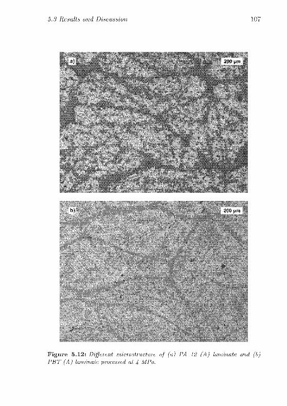
5.3 Results and Discussion 107
Figure 5.12: Different microstructure of (a) PA-12 (A) laminate and (b)PBT (A) laminate processed at 4 MFa.

108 Laminate Quality of Stamp Formed Commingled Yarns
less than one minute, so that deterioration of laminate properties due to
polymer degradation may be negligible.
Conclusions
Stamp forming of commingled yarn intermediate materials with different
blending qualities and resin polymers has been examined at a number of
processing conditions. It is shown that laminates with low void contents
can only be obtained if yarns with extraordinary blending quality arc
employed. The measured void contents are compared with those com¬
puted using an impregnation model suggested by Bernet et al. [12]. Good
agreement with the model is only found in case of laminates producedfrom yarns with intermediate blending quality and consolidated at the
lower end of the range of applied processing pressures. Laminates stamp
formed from yarns with highly intimate commingling exhibit much lower
void contents as compared with the computed voidage. The discrepancyis attributed to model assumptions not being appropriate to the present
yarn architectures and investigated consolidation pressure levels. The
stamp forming of unimpregnated intermediate materials is capable of
delivering laminates with as low voidage as 1 %, given the intermediate
material exhibits extraordinarily mingling of resin and reinforcement fi¬
bres. Based on the results presented above, a new yarn prototype with
commingled PBT and carbon fibres is currently under development. The
new prototype will feature an optimised carbon fibre sizing to improve
fibre/matrix adhesion, and the fibre length distributions of PBT and
carbon fibres are adapted to each other within the limits of possibilityto further enhance the blending quality.
References
[1] L. Ye, K. Friedrich, J. Kastei, and Y.-W. Mai. Consolidation of
unidirectional cf/peek composites from commingled yarn prepreg.
Composites Science and Technology, 54(4):349 358. 1995.
[2] II. Ilamada. Z.-I. Maekawa. N. Ikegawa, and T. Matsuo. Influence of
the impregnation property on mechanical properties of commingled
yarn composites. Polymer Composites, 14(4):308 313, 1993.
5.3 References 109
[3] B. Lauke, U. Bunzel. and K. Schneider. Effect of hybrid yarn struc¬
ture on the delamination behaviour of thermoplastic composites.
Composites Part A, 29A:1397 1409, 1998.
[4] P. McDonnell, K. P. McGarvey. L. Kochford, and C. M. O'Bradaigh.
Processing and mechanical properties evaluation of a commingled
carbon-fibre/pa-12 composite. Composites Part A, 32:925-932,2001.
[5] J. Vendramini. C. Bas, G. Merle, P. Boissonnat, and N. D. Alberola.
Commingled poly(butylene terephthalate)/unidirectional glass fiber
composites: Influence of the process conditions on the microstruc¬
ture of poly(butylene terephthalate). Polymer Composites, 21:724
733, 2000.
[6] G. Bontemps. private communication, 2002. Scbappe Tcchniqcs,F-01800 Charnoz, France.
[7] I. Y. Chang and J. K. Lees. Recent developments in thermoplastic
composites: A review of matrix systems and processing methods.
Journal of Thermoplastic Composite Materials. 1:277 294, 1988.
[8] R. Beyreuther, II. Brunig, and R. Vogel. Preferable filament diam¬
eter ratios of hybrid yarn components for optimized longfiber rein¬
forced thermoplastics. International Polymer Processing. 17(2): 153157. 2002.
[9] N. Bernet, Y. Michaud, P.-E. Bourban, and J.-A. E. Mânson. Com¬
mingled yarn composites for rapid processing of complex shapes.
Composites Pari A, 32:1613-1626, 2001.
[10] U. I. Thomann and P. Ermanni. Rapid thermoforming of com¬
mingled yarn a direct way from soft textiles to structural parts.
In S. V. Hoa. A. Johnston, and J. Denault, editors, Design, Man¬
ufacturing & Application of Composites: Proceedings of the Third
Canadian International Conference on Composites, pages 229 236,
Lancaster. PA, USA, 2001. Teclinomic Publishing Company, Inc.
[11] D. P. Bloch. Solvents and non solvents for polymers. In J. Braiidrup.E. H. immergut. and E. A. Grulke, editors. Polymer Handbook. 4th
Ed., page Vll/515. John Wiley & Sons, Inc., New York, 1999.
[12] N. Bernet, V. Alichaud. P.-E. Bourban, and J.-A. E. Mânson. An
impregnation model for the consolidation of thermoplastic compos¬
ites made from commingled yarns. Journal of Composite Materials,
33(8):751 772, 1999.
110 Laminate Quality of Stamp Formed Commingled Yarns
[13] AL D. Wakeman, T. A. Cain, C. D. Rudd, R. Brooks, and A. C.
Long. Compression moulding of glass and polypropylene compositesfor optimised macro and micro mechanical properties 1 commin¬
gled glass and polypropylene. Composites Science and Technology,58:1879-1898, 1998.
[14] J. A. Barnes and F. N. Cogswell. Transverse flow processes in contin¬
uous fibre reinforced thermoplastic composites. Composites, 20:38
42, 1989.
[15] M. Pellow-Jarman and M. Hetem. Comparison of the thermal degra¬dation products of poly(butylcne terephthalate) and flame retardant
poly (butylène terephthalate) using a pyrolysis ftir cell. Polymer
Degradation and Stability, 47:413-421, 1995.
[16] A. Frick and C. Stern. Verweile mit Eile: Zu lange Verw-eilzeiten bee¬
influssen die Eigenschaften von PBT-Bautcilen. Kunststoffe, 7:46-
48, 2002.

Chapter 6
Heat Transfer during
Stamp Forming
6.1 Introduction
Stacks of commingled yarn fabrics can be shaped, consolidated, and
cooled to release temperature in one single process step [1]. To ensure
thorough consolidation, however, the blending has to be extremely in¬
timate as to provide the shortest possible flow distance for the viscous
molten polymer fibres to impregnate the reinforcement fibres [2]. It was
also reported that the laminate quality in terms of mechanical proper¬
ties can be enhanced, if thermally insulating moulds rather than metallic
tools are employed [3].
Stamp forming is a highly non isothermal process. For the sake of pro¬
cess optimisation and quality control it is necessary to gain knowledgeabout the laminate cooling during moulding. Hence, it is required to ac¬
cess a mathematical description of the moulding/consolidation/coolingstep of the process. The development of such a model requires to solve
the heat transfer equation, which was performed by several authors for
a number of neat and reinforced polymers and different processing con¬
ditions [4-7].
The present work employs the finite differences method to numericallysolve the thermal equation of energy conservation in one dimension to

112 Heat Transfer during Stamp Forming
predict the temperature profile through the thickness of a primarily
unimpregnated carbon fibre/poly(laurolactam) laminate during consol¬
idation as observed in the stamp forming process. As far as possible,the material parameters such as specific heat, thermal conductivity, and
density of laminate components as well as the moulding tool were consid¬
ered to vary with temperature. Further to considering variable material
parameters, the standard finite differences approach is expanded to ac¬
commodate variable laminate density and thermal conductivity due to
progressing consolidation at the formulation of the heat transfer equa¬
tion.
6.2 Experimental Methods
Thermal material properties such as specific heat of the laminate as well
as the PEEK plates, and the crystallisation kinetics of PA-12 were deter¬
mined by differential scanning calorimetry. The experimental approachfor specific heat measurements and respective data for the different com¬
ponents involved in the stamp forming process have already been pro¬
vided in Sections 3.1 and 3.2.1. The same laboratory equipment w7as used
to estimate isothermal crystallisation kinetics and its related parameters
such as the dependence of crystallisation temperature on cooling rate
and the latent heat of crystallisation.
6.2.1 Détermination of Crystallisation Kinetics and
Related Parameters
For isothermal crystallisation kinetic measurements cubes of about 6 mg
weight of Carbon fibre/PA 12 laminates with a fibre volume fraction
of 0.5 were put in aluminium pans without covers. Prior to isothermal
crystallisation the samples were held at 220 °C for 3 min to remove
any nuclei. Then the sample was cooled at a rate of 12 °Cs_1 to the
required crystallisation temperature, which was maintained until poly¬mer crystallisation was concluded. The run was stopped only after the
signal has well returned to the baseline. Crystallisation temperatures
ranged from 159.2 °C to 165.2 °C and the temperature interval from
one measurement to the next was 1 °C.Each run was performed with a
new sample to prevent from degradation influencing the measurement.
Latent heat of crystallisation and the dependence of crystallisation tem¬
perature on cooling rate of PA 12 were obtained by quenching polymer
6.3 Heat Transfer Model 113
disks of roughly 6 mm diameter by 0.16 mm thickness weighing approx¬
imately 3 nig, which were cut from a PA 12 sheet. The samples were
heated to 220 °C and held at this temperature for 3 min before subse¬
quently quenching to 100 °C at various cooling rates, ranging from A.
to !°Cs-'.
6.2.2 Stamp Forming of Commingled Yarn Preforms
Four layers of woven fabric of carbon and poly(laurolactam) (desig¬nated as PA 12 hereafter) fibre commingled yarn were heated between
two infra red radiation fields as described in Chapter 4 and subse¬
quently to reaching the desired laminate temperature transferred to a
hydraulic hot press, where, subsequently, the fabric stack was subjectedto stamp forming to result in a consolidated flat laminate. The com¬
mingled yarn was a blend of Tenax® HTA carbon fibres and EMS
Chemie Grilamid® L16 PA-12 fibres at a carbon fibre mass fraction
of 0.64, resulting in a fibre volume fraction of 0.5 in the thoroughly con¬
solidated laminate. The mould consisted of two rectangular poly[4,4'-(p-phenylenedioxy)-diphenylene ketone] (better known under its trivial
name poly(ether ether ketone) and designated as PEEK hereafter) platesof 16 mm thickness mounted on the press plates. The applied consoli¬
dation pressure was 4 MPa. Between each layer of the laminate as well
as on the mould surface and the press plate the temperature was mon¬
itored and recorded continuously by means of K type thermocouples.The experimental set up is illustrated schematically in Figure 6.1.
6.3 Heat Transfer Model
6.3.1 Theoretical Considerations
As the viscosity of the thermoplastic matrix is high and the fibres restrict
macroscopic resin flow, the cooling of a flat laminate of temperature T
with thickness x much smaller then its length and width can be handled
as a simple problem of one dimensional heat conduction. The thermo¬
dynamic equation of energy conservation applies:
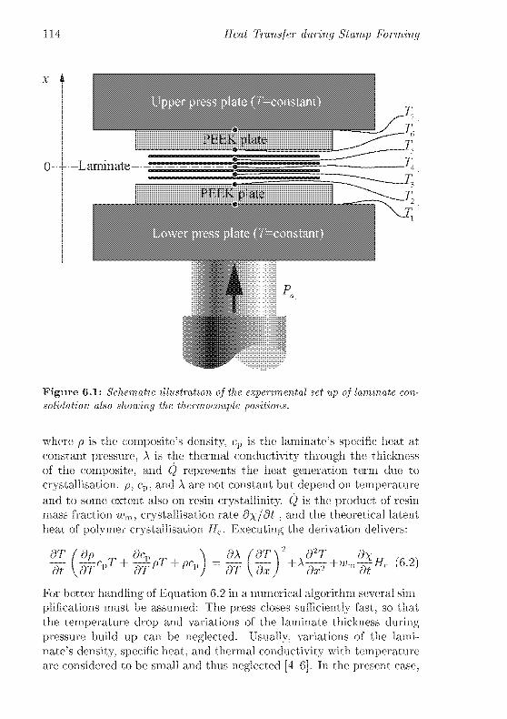
114 Heat Transfer during Stamp Forming
x 4
-Laminate
P„
Figure 6.1: Schematic illustration of the experimental set up of laminate con¬
solidation also showing the theimocouple positions
where p is the composite's density, cp is the laminate's specific heat at
constant pressure, A is the thermal conductivity through the thickness
of the composite, and Q repiesents the heat geneiation term due to
ciystallisation p. cp, and A are not constant but depend on temperature
and to some extent also on resin crystallinity. Q is the product of resin
mass fraction wm, crystallisation rate d\jdt ,and the theoretical latent
heat of polymer crystallisation IR. Executing the derivation delivers:
OT
dt
dprp
ärCpl9CP
rp
W1 P<PdT
or
dx
82rl d\+ *»-T+«'m-£#c (6.2)
dx2 dt
For better handling of Equation 6.2 in a numerical algorithm several sim¬
plifications must be assumed: The press closes sufficiently fast, so that
the temperature drop and variations of the laminate thickness during
pressure build up can be neglected. Usually, variations of the lami¬
nate's density, specific heat, and thermal conductivity with temperatuie
are considered to be small and thus neglected [4 6]. In the present case.

6.3 Heat Transfer Model 115
however, the laminate contains a significant amount of air, which is grad¬
ually decreasing during consolidation and cooling. Hence, the laminate
density as well as the thermal conductivity change with progressing con¬
solidation. Particularly at the beginning of the stamp forming process
the change of density is expected to be very articulate and, hence, the
usual assumption of the density gradients being negligible is inappropri¬
ate. Although the direct stamp forming of unconsolidated hybrid yarns
is described in [7] this problem w7as not mentioned by the authors. Here,the laminate density is variable with temperature and laminate coordi¬
nate and the thermal conductivity is assumed to vary with temperature
only, i.e., the spatial gradient of the thermal conductivity is neglected.With these preliminary assumptions Equation (6.2) can be simplified as:
°Ptm dT\ \d2T j. d*n frv
diT+p-dt)=Xd?+Wm'dtnc
(6'3)
6.3.2 Spatial and Temporal Discretisation
Equation (6.3) is discretised in time and space as schematically shown
in Figure 6.2. The temporal and spatial derivations are linearly approxi¬mated within the temporal increment At and the spatial increment Aa;,
namely:
r.'+1 - -rf a»=
rf+1. - ».'f~Kt ' dt
~~
At
„,„rk+l Tk+i -V'm Tk+1 ot^+I , tHI
dT j_ >i+i-
P d"I j_ P+i-
ZP + P-i
1TF~ Si ' &^~ Ä?
(6.4)
Replacing the temporal and spatial derivatives of temperature and den¬
sity by their corresponding discrete terms as given in Equation (6.4) one
obtains after basic transformation an implicit solution for the lami-

116 Heat Transfer during Stamp Forming
%
o
ao
43
i+l-
At
T1
. ; •
b\ hi h \
i i i
• =k =+-
rl
'+1 i
rA-lj
1+1 j
t\
i ;
»! r*, i
*-i
1 Laminate/Tool-
Tk+l i Interface
i+l i
Ax
rpk+l'l-l
li i ii
-?i-
*+l Time
Figure 6.2: Schematic illustration of the temporal and spatial discretisation.
nate temperature at position i and time k:
Tf+a.Q1; = 6,T,":+' +c,7-.'+1 +f»,T,'+-'
'- = 7^,_
~\kAt
Pi Pi cp
(6.5)
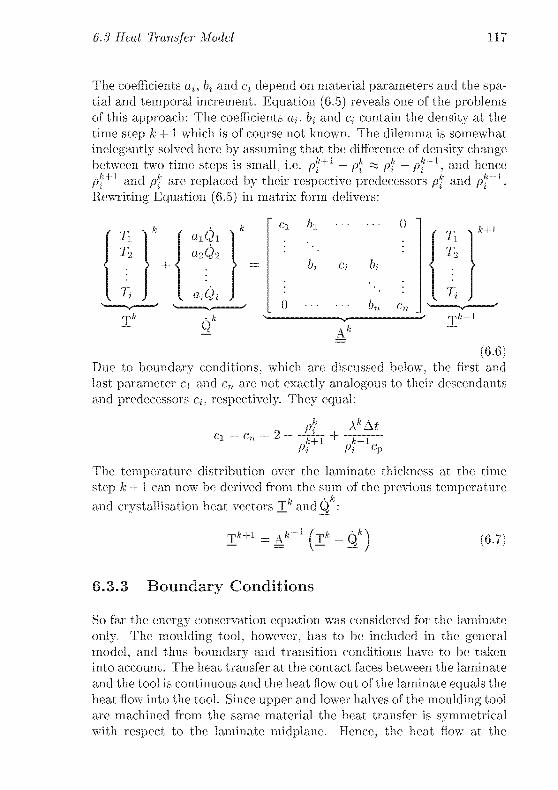
6.3 Heat Transfer Model 117
The coefficients at, bt and c\ depend on material parameters and the spa¬
tial and temporal increment. Equation (6.5) reveals one of the problemsof this approach: The coefficients at, b% and c, contain the density at the
time step k+ 1 which is of course not known. The dilemma is somewhat
inelegantly solved here by assuming that the difference of density change
P%k+\between two time steps is small, i.e
Rewriting Equation (6.5) in matrix form delivers:
P, ~ Pi-
Pi "L. and hence
and pk aie replaced by their respective predecessors pk and pt
f rji \
' 1
k
r oiQi }'Ti a2Q-2
. f +1=
,
T,.
s
.a,Qt J
C]_
c, b,
k-i
TKQ
Tk+i
(6.6)Due to boundary conditions, which are discussed below, the first and
last parametei ci and rn are not exactly analogous to their descendants
and predecessors ct, respectively. They equal:
ClPi
Pifc+i
+\ktd
Ptlcp
The temperature distribution ovei the laminate thickness at the time
step k+\ can now be derived from the sum of the previous temperature
and crystallisation heat vectors T* and Q'
:
-.A.+ 1 a1-1(:t/ + q1) (6.
6.3.3 Boundary Conditions
So far the energy conservation equation was considered for the laminate
only. The moulding tool, however, has to be included in the generalmodel, and thus boundary and transition conditions have to be taken
into account. The heat transfer at the contact faces between the laminate
and the tool is continuous and the heat flow out of the laminate equals the
heat flow into the tool. Since uppei and lower halves of the moulding tool
are machined from the same material the heat transfer is symmetricalwith icspect to the laminate midplane. Hence, the heat flow at the
118 Heat Transfer during Stamp Forming
position x = 0 is null. The press plates have a much greater thermal
mass than the moulding tool and the laminate together. Fuithermore
their temperature is maintained constant electronically. It is therefore
reasonable to assume constant temperature at the interfaces between
press plate and tool. Insertion of the symmetry condition delivers:
%f(T1k+ltâ-A-1)+fiî(TÏ~l-T!>))
rpk+ l___
Tk~l= xk 2 tl +Qi
Likewise, one obtains on insertion of the transition condition:
Si H 23?
(6..
xi#î-(\ + \)Ttl + xrtzl(6.9)
A.Z~ Qt
where symbols labelled with ~ refer to parameters belonging to the
moulding tool. The spatial and tempeiature subscripts conesponds to
the definition as given in Figure 6.2.
6.4 Material Parameters
Alaterial parameters of composite laminates have already extensivelybeen discussed in Chapter 3. Due to the here applied pressure in con¬
trast to the non or only slightly pressurised fabric ply stacks consideied
in Chapter 4. effects of progressing consolidation on the thermal conduc¬
tivity and the density have to be taken into account.
6.4.1 Thermal Conductivity
The laminate's thermal conductivity has been discussed in detail in Sec¬
tion 3.2.3. Thermal conductivity variations as a result of progressingconsolidation are taken into account by applying the consolidation model
of Bernet et al. [8] at each time step and then calculating the laminate's
conductivity according to Equations 3.8 and 3.9. Contrary to the mod¬
elling of Remet et al. not only two different fibre bundle si/es but a
statistical distribution as given in general form in Equation (2.39) is

6.4 Material Parameters 119
used, incorporating 20 fibre bundle size classes. The parameters to cal¬
culate the frequency of occurrence of a bundle size were estimated from
micrograph]cal observations of a representative yarn cross section as il¬
lustrated in Figure 5.2 on page 87. The maximum fibre bundle size was
assumed to contain 180 reinforcement fibres, the predictand was set to
/i* = In 50, and finally the square root of the variance was estimated to
equal s = 1.6.
For calculation of the laminate's thermal conductivity, knowledge of the
fibre volume fraction in unimpregnated areas is necessary. This can be
done by means of Equation (2.10) as presented in Chapter 2 on page 26.
To obtain the fibre volume fraction as a function of the fibre bed pressure
it is necessary to numerically solve Equation (2.10). Non-linear solvers,however, drastically prolong the computing time. To accelerate compu¬
tation, the fibre volume fraction was here obtained in explicit form bycurve fitting of Equation (2.10) to the following expression:
/
ff(P)=uo+(wf(P)-un)
ax b
c\ d(6.10)
with
v0 = 0.737,
a = 4.704,
P:
b-
:8.41 [MPa]: 1.759,
V((P)c -
0.780,
0.6924, d = 3.920
Choy et al. [9] measured the thermal conductivity of PEEK at tempera¬
tures ranging from 150 to 500 K. The authors report a thermal conduc¬
tivity of 0.243 W m[ K~l and 0.259 Wm' K '
at 295 K for amorphousand crystalline PEEK, respectively. The crystalline volume fraction
amounted to 0.3. Material parameters the here employed Tecapeek®
plates as provided by the material supplier' essentially agree with these
values within the error margin of experimentation. According to Choyet al. [9] the thermal conductivity of PEEK increases almost linearlywhen the temperature is raised until the glass transition temperature is
reached, whereupon the thermal conductivity decreases slightly. As the
changes are small within the temperature interval of present interest, a
constant value of 0.284 Wm-' K"1 was assumed here.
'Ensinger GmbH, Rudolf Diesel Strasse 8, D 71157! Nufringen, Germany

120 Heat Transfer during Stamp Forming
6.4.2 Crystallisation Kinetics
In contrast to Chapter 4, where the temperature of fabric ply stacks was
predicted according to analytical solutions of the heat transfer equationand the melting enthalpy was not taken into account, effects of crys¬
tallisation on the laminate temperature cannot be neglected here, if it
is desired to obtain process relevant information such as determination
of the elapsed time until the laminate has solidified and can be safelyremoved from the mould. This, however requires knowledge of the poly¬mer's latent heat of crystallisation and the crystallisation rate under
processing conditions.
The latent heat of crystallisation of the neat resin was reported to
decrease logarithmically with increasing cooling rate [10]. Such a be¬
haviour, however, was not observed here. The crystallisation enthalpyof PA 12 at the presence of 50 volume % carbon fibres was not signifi¬
cantly affected by cooling rates ranging from to | °C s_1. It amounts
to 53 ± 1 J g"1. Increasing cooling rates, however, lower the crystallisa¬tion temperature, i.e.. the higher the cooling rate the greater the amount
of super-cooling AT = T°—Tc necessary to induce crystallisation. T° is
thereby the equilibrium melting temperature of a perfect polymer crystaland Tç is the crystallisation onset temperature. Evidently, the measured
crystallisation onset temperatures obey a simple power law7 function of
the cooling rate (Figure 6.3):
TC[°C\ = 155.2 (§p with § [^] = [£....,§] (6-n)
Although non isothermal treatment of crystallisation kinetics would be
necessary to represent the heat source term in Equation (6.2) correctly,
only isothermal kinetics were considered to give results of sufficient accu¬
racy for present purposes. This is basically motivated due to the coolingcurves of stamp formed laminates as reported previously [2] showingthat crystallisation occurs in the flat region of the cooling curve, where
the moulding tool temperature is approached. It therefore seems to be
justified to employ isothermal modelling if relatively high tool temper¬
atures arc considered. Analysis of the isothermal crystallisation exper¬
iments of CF/PA-12 laminate samples containing 64 weight-% carbon
fibres showed that the crystallisation rate is somewhat asymmetric with
respect to the peak maximum as exemplified for Tc = 162.2°C in Fig¬ure 6.4. This behaviour is thought to result from two different superim¬
posed nucleation mechanisms: (1) heterogeneous nucleation occurringat the interface between carbon fibre surface and polymer melt, and (2)

6.4 Material Parameters 121
175
150
l ' ' ' l 1 ' l -Î ! 1 ! 1 ! 1 ! 1 1—
_J ! I ! I ! I ! I I I ! I I I ! I I ! ! I I ! ! ! I ! ! ! I L-
1 1.2 1.4 1.6
,,-i.
0 0.2 0.4 0.6 Oi
Cooling Rate (-ôT/ôt) [°C-s ]
Figure 6.3: Temperature of crystallisation onset vs. cooling rate.
combined heterogeneous and homogeneous nucleation within the bulk of
the polymer melt. Owing to the vast surface provided by the carbon
fibres, the former is assumed to happen faster than the latter, yieldingan asymmetric crystallisation rate peak with the steep flank being at the
beginning of crystallisation. The degree of symmetry of the conversion
rate curve is determined by the Avrami exponent n, which in fact re¬
flects the mode of nucleation. A value of n = 2 delivers Gauss bell curve
and represents instantaneous and homogeneous nucleation and discoid
or rod like crystal growth. Other values of n have been related to dif¬
ferent kinds of crystal growth such as instantaneous nucleation and rod
like crystal growth (n = 1), instantaneous and homogeneous nucleation
and spherulitic or discoid crystal growth (n = 3), and homogeneous
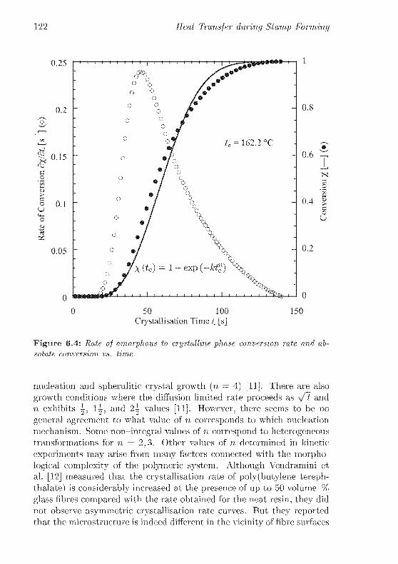
122 Heat Transfer during Stamp Forming
0 50 100 150
Crystallisation Time tc [sj
Figure 6.4: Rate of amorphous to crystalline phase conversion rate and ab¬
solute conversion vs. time.
nucleation and spherulitic crystal growth (n = 4) [11]. There are also
growth conditions where the diffusion limited rate proceeds as \[t and
n exhibits \, \\, and 2| values [11]. However, there seems to be no
general agreement to what value of n corresponds to which nucleation
mechanism. Some non-integral values of n correspond to heterogeneoustransformations for n = 2,3. Other values of », determined in kinetic
experiments may arise from many factors connected with the morpho¬
logical complexity of the polymeric system. Although Vendramini ct
al. [12] measured that the crystallisation rate of poly(butylène tereph¬
thalate) is considerably increased at the presence of up to 50 volume %
glass fibres compared with the rate obtained for the neat resin, they did
not observe asymmetric crystallisation rate curves. But they reportedthat the microstructure is indeed different in the vicinity of fibre surfaces
6.4 Material Parameters 123
compared to the bulk polymer, which is evidence for the different nucle¬
ation mechanisms. Despite the ambiguity associated with the Avrami
exponent n. the Avrami model to express the degree of conversion \ in
terms of elapsed crystallisation time was used here:
X(A)=l-exp(-A;tc") (6.12)
where k is the Avrami coefficient, n is the Avrami exponent as discussed
above, and tc is the crystallisation time, i.e. fc is null as soon as the
temperature is equilibrated at T = Tc.
As pointed out above the cooling rate determines the crystallisation on¬
set temperature. In the present case, however, the cooling rate is not
constant but decreases when the mould temperature is approached. In
the thermal model it is thus necessary to consider the present cooling rate
and laminate temperature to obtain a criterion for crystallisation onset,
i.e. it is initially not known at which temperature or after how much
elapsed time the polymer starts to crystallise. Therefore the parame¬
ters of Equation (6.12) have to be represented continuously as functions
of the variable crystallisation onset temperature. The dependence of
these parameters on temperature was obtained by curve fitting of Equa¬tion (6.12) to the measured isothermal crystallisation data at various
crystallisation temperatures. It was found that n assumes a constant
value of 2 within the present range of crystallisation temperatures, and
k fits to the expression:
k = 1.71 • 10~2(TC [°C] - 155.7)~2 (6.13)
Together with knowledge of the total latent heat of crystallisation AIR,the heat source term as a function of crystallisation time as it appears
in the thermal equation of energy conservation Q is determined as
^à [i] = 2Hcexp (-ki) wmAIR (6.14)
Table 6.1 summarises the above presented numerical relationships be¬
tween material parameters and processing conditions during thermo¬
forming and those already discussed in Chapter 3, together with ref¬
erence to their occurrence in respective Equations. A flow chart of the
main loop is given in Figure 6.5. It illustrates the computer program'sbasic components and the sequence of calculations.

124 Heat Transfer during Stamp Forming
V „H Hi | ?' ^
3
53
3i i
»
Wi I
!
*-
i 1
co
5oco
'S?
'S?H-1
to
en
ocro
CR CK!
!
oo
oo
co
co
to oo
o oo to
to
2 o
oo
I
sàto
n
+o
toto
k; Zi
H H
V IA
.H nH
K2
oo't
o
I—*
O
|
o
1CO
J3
+o
in00
O
rf-» CO W
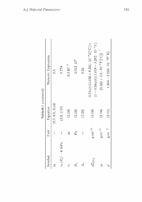
6.4 Material Parameters 125
+E>
o
o !O O
î-H
]h ^L
ooo 0 h
so CN -^
o !—1
o bsO
iO T~H j ] ^H
"*f co Os 1
o
1-o
o s lO
06oo
o
O
iO>
ö
cöT-H ci
1
o
o
c-i
o
oi
lO
p^
+
ID
Ö
1
Ö
3 1
Öo
£
pcö
t-
cö
o
c-i
co
CN CN
co
co
lO
cô
O
42
ce er *!
I^
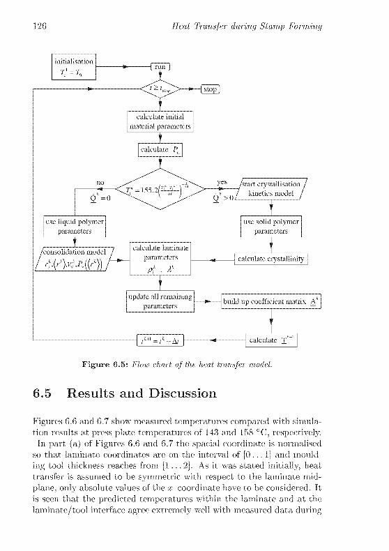
126 Heat Transfer during Stamp Forming
initialisation
t=T„
Q=0
use liquid polymer
parameters
Ï/consolidation model
WKW))
calculate initial
material parameters
calculate P,
calculate laminate
parameters
P, ,/•
update all remaining
parameters
1 st0P J
tK+i=tk+At
yj)s /start crystallisation.•J 77 kinetics model /Q >(n
use solid polymer
parameters
calculate crystallinity
build up coefficient matrix A
calculate TT
Figure 6.5: Flow chart of the heat transfer model.
6.5 Results and Discussion
Figures 6.6 and 6.7 show measured temperatures compared with simula¬
tion results at press plate temperatures of 143 and 158 °C, respectively.In part (a) of Figures 6.6 and 6.7 the spacial coordinate is normalised
so that laminate coordinates are on the interval of [0... 1] and mould¬
ing tool thickness reaches from [1 .. .2]. As it was stated initially, heat
transfer is assumed to be symmetric with respect to the laminate mid¬
plane, only absolute values of the a; coordinate have to be considered. It
is seen that the predicted temperatures within the laminate and at the
laminate/tool interface agree extremely well with measured data during
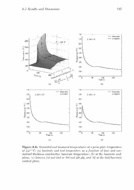
6.5 Results and Discussion 127
(di
Figure 6.6: Simulated and measured temperatures at a press plate temperature
of 143°C: (a) laminate and tool temperature as a function of time and nor¬
malised thickness coordinates: laminate temperatures (b) at the laminate mid¬
plane, (c) between 1st and 2nd or 3rd and 4th ply, and (d) at the. tool/laminate,contact plane.
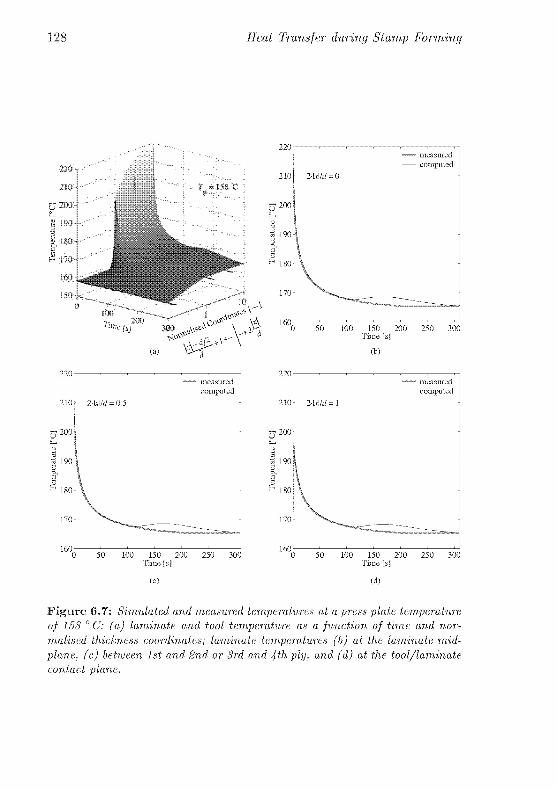
128 Heat Transfer dvring Stamp Forming
measured
computed
"n 2m ~^~ .Vot«***6 \A 160
r'fflefi,j 300 mP& \ „ip: 0 50 100 150 200
Tune [s]
(b)
measured
computed
"0 50 100 150 200 250 300
Time \s]
(c)
190
• measured
computed
100 150 200
Time [s]
(d)
Figure 6.7: Simulated and measured temperatures at a press plate temperature
of 158° C: (a) laminate and tool temperature as a function of time and nor¬
malised thickness coordinates; laminate temperature s (b) at the laminate mid¬
plane. (c) between 1st and 2nd or 3rd, and 4th ply. and, (d) at the tool/laminatecontact plane.
6.5 Results and Discussion 129
the entire process in case of a press plate temperature of 143 °C, whereas
for a press plate temperature of 158 °C the temperature rise due to crys¬
tallisation is not observed in the experiment but predicted by the model.
This indicates, that the here employed simplified crystallisation kinet¬
ics model is inaccurate for high crystallisation temperatures. But other
than the discrepancy in the area of predicted crystallisation, simulated
temperatures also coincide with experimental data.
The effect of a mould material featuring low thermal conductivity is also
visible in Figures 6.6 and 6.7: Initially, the heat is transferred quicklyto the mould surface. Then, as a result of the low thermal conductivity,heat transfer through the PEEK plates to the press plates is slow, so
that even after 180 s the temperature difference between laminate/tooland tool/press plate interfaces is still more than 10 °C for 143 °C press
plate temperature. From a technical point of view it would be interestingto know up to which thickness the insulating effect of the PEEK platesis efficient. Figure 6.8 provides such data. Obviously, the time the
laminate midplane requires to cool to a fixed temperature of 167 °C
does not significantly increase for insulator plates thicker than about
10 mm.
As a byproduct the here presented thermal model also delivers the lam¬
inate void content, which is required to calculate the instantaneous lam¬
inate density and thermal conductivity. The laminate void content as
function of processing time is shown together with the resin viscosity in
Figure 6.9 for both investigated press plate temperatures.
The influence of fibre intermingling quality on mechanical properties of
the laminate was discussed in Chapter 5. It was empirically demon¬
strated that increased blending quality yields lower void content and,
hence, improves mechanical properties of the stamp formed laminate.
It is therefore interesting to investigate the impact of blending qualityon the consolidation behaviour by means of the integrated heat trans¬
fer/consolidation model. Figure 6.10 shows the temperature at the mid¬
plane of laminates stamp formed from yarns with different yarn architec¬
tures. The solid line represents the void content at the laminate midplaneof a laminate made from a yarn with the characteristics of PA 12 (A)
yarn as given in Chapter 5, which is the same as used to weave the here
employed fabrics. The other curves correspond to yarn parameters of
PA 12 (B), and PBT yarn as also introduced in Chapter 5, respectively;
and, finally, the lowermost curve results from a hypothetical yarn with
optimal commingling, i.e. assuming a constant fibre bundle size that

130 Heat Transfer during Stamp Forming
230
220
Insulator Thickness d [mm]
10 15 20 25 30 35
,32 mm
55
50
- 45
- 40
35
- 30
25
20
15
200
Uc
r-so
Figure 6.8: Time the laminate requires to cool to 167 °C at a press plate
temperature of 150°C.
equals the ratio:
rj ?/f(6.15)
where rm is the radius of the polymer fibres. Using the radius of PA-12
fibres rm « 1.15 • 10""° m and setting the fibre volume fraction 0.5, the
optimum fibre bundle contains approximately 11 fibres. Statistical yarn
characteristics as employed to obtain the curves shown in Figure 6.10 are
summarised in Table 6.2. The symbols used in Table 6.2 refer to those
given in Equation (2.39). If the limit of porosity to define "satisfactorylaminate quality" is somewhat arbitrarily set to 5 %. only the PBT yarn
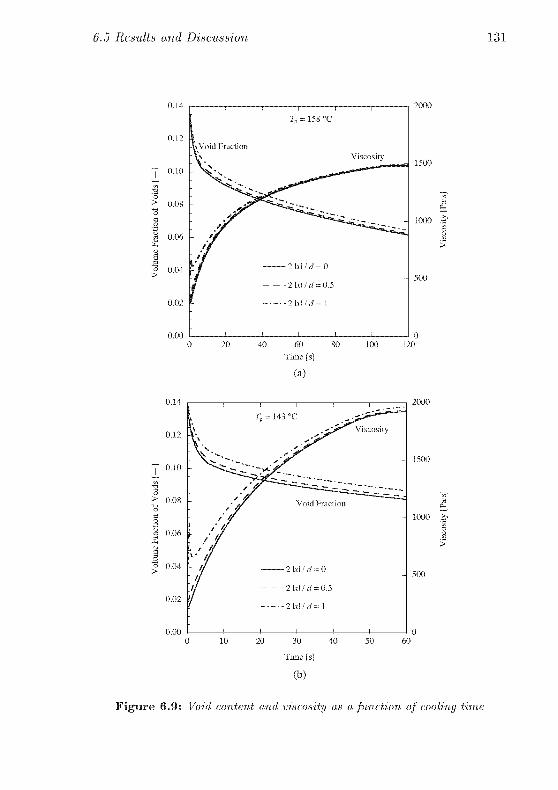
6.5 Results and Discussion 131
0.12
0.08
0.02
1 ! I !
Zp = 158 °C
1
-U Void Inaction
V Viscosity
- x>
**r '^^"^^i--.^"^Sî*a*ffl!
:-i^Äi-;i^ -
/f'
*f'
iE
2l>l'rf=0
2Lil/ri = 0.5
2\\\ld= 1
1 ! I ! 1
looo S
500
0
0 20 40 60 80 100 120
lime [s]
(a)
0.12
> 0.08
0 02
VTv = 143 °C
V .^/f^ ViscosityT\
^j
/ //
?
f1?
s 0*
Void Fraction
i ; /I•y if- il 2 bel ' d --= 0
i-
u - - - 2 lil ; d --= 0.5
= 1
i 1 I 1 1
1000 &
500
0 10 20 30 40 50
Time [s]
(b)
Figure 6.9: Void content and viscosity as a function of cooling time

132 Heat Transfer during Stamp Forming
15
I
&
^
a
Sao
U
"2'o>
10
— Aff = 180, u= in 50, s =1.6max
'
Tp = 150 °C
Arf = 150,//* = In 30, s =1.6max
- N( =80,/i* = lnll,,v= 1.8
i\ max^
!K — N = constant =11
It'"- \. -
' * '•- ^"""""-»«^^i * ''••. ^"""---—^.; \i- \
1 \ '"••-.i \
X
\ \
X^
X
\X
X, <*»
'x_ "a.'
X**
*»'
X ****"•**'
X'
X'
X
"*"*""
««
<*»,""**
*»,
'
***,
*<*,
«*B,
10 20 30 40 50
Time [s]
60 70 80
Figure 6.10: Void content at laminate midplane as function of cooling time
for different yarn architectures at a press plate Temperature Tp = 1*50 °C.
(— in Figure 6.10) undergoes this limit for these processing conditions.
This clearly demonstrates the importance of commingling quality for
the successful use of unconsolidated commingled varn preforms for the
stamp forming process.
In Chapter 5 reservations about the validity of Bernet's consolidation
model for extremely well intermingled fibre yarns have been made. One
of the problems might lay in the selection of the permeability calculation
according to Gebart [13] rather than according to the Carman Kozeny
equation or the modified Carman Kozeny after Gutowski et al. [14]. Fig-

6.5 Results and Discussion 133
Table 6.2: Statistical yarn characteristics
Yarn Parameter
ii* s- <VfF * J '
ma
PA-12 (A) In 50 1.6 180
PA-12 (B) In 30 1.6 150
PBT In 11 1.8 80
ATl = constant.6 i/f = 0.5 11
"Number of fibres contained within the largest observed fibre bundles
'calculated according to Equation (6.15) for rm = 1.15 • 10""° m, which equals the
radius of PA 12 fibres (see Section 5.2.1).
ure 6.11 demonstrates the effect of different permeability calculations on
the evolution of void content and permeability during stamp forming of a
yarn with the characteristics of the previously introduced PBT yarn at a
press plate temperature of 143 °C. Using the Carrnan-Kozeny equationto estimate the fibre bed permeability, the consolidation model predictsalmost instantaneous fibre impregnations, which can hardly be a proba¬ble scenario. Considering the dot and dash line in Figure 6.11 obtained
with the permeability calculated according to Equation (2.7), the resid¬
ual void content amounts to about 1 %. which is approximately the
same value as experimentally obtained for PBT yarn at similar coolingconditions (see Section 5.3). Obviously, Gebart's permeability calcula¬
tion according to Equation (2.8) overestimates the influence of fibre bed
compaction on permeability in case of small fibre bundles.
The use of thermally insulating moulds made from high temperature re¬
sistant plastics such as PEEK can be problematic in that such materials
arc extremely costly and the dimensional stability under thermal load is
not satisfactory. Therefore, it would be interesting from a technical pointof view to stamp form commingled yarn preforms between conventional
steel moulds. Figure 6.12 provides simulated void content and viscositydata for commingled yarn preforms with the commingling characteristics
of type PBT yarn stamp formed in steel moulds at a press plate temper¬
ature of 160 °C. For steel the following temperature independent mate¬
rial parameters were assumed: thermal conductivity À = 75 WmK-1,specific heat cp = 465 JkgK1, and density p = 7870kg m3. Due to
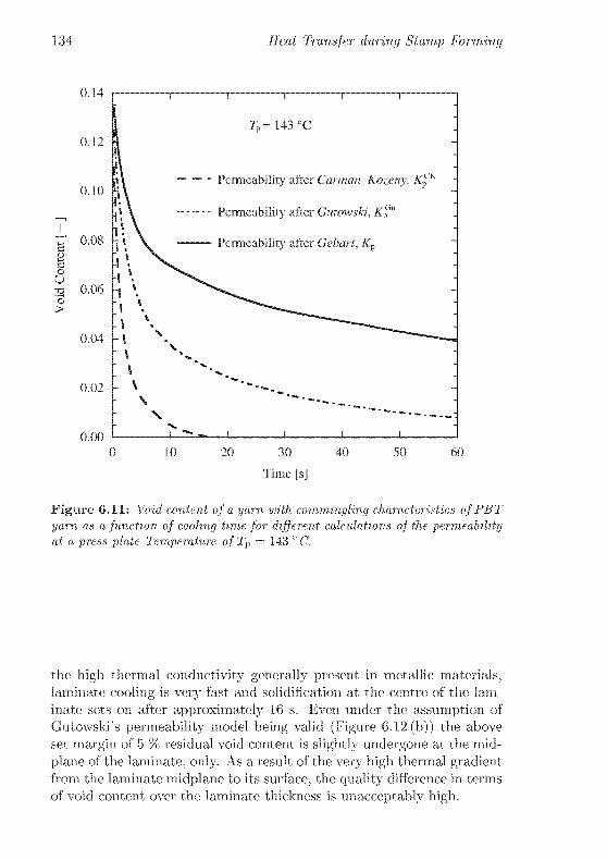
134 Heat Transfer during Stamp Forming
0.14
0.12
0.10
r 0.08 fti
1o
U
3 0.06'o>
0.04
0.00
i 1 1 1 1
Tp=143°C ^
i\-
ji\ Penneability after Carrnan-Kozeny, K^'K
Permeability after Gutowski. A'pGui'A -
• \ Permeability after Gebart, Kp
J1. N '.
-I \ .
1 \ '»x«^^
"j ». ^"^x***^,^^
"l \,
\-1
%^-
1 X
\Bx
"
"X
-\
"x,.
\ ""*---
\" X,
.1 1 1 1
10 20 30
Time [s]
40 50 60
Figure 6.11: Void content of a yarn with commingling characteristics of PBT
yarn as a function of cooling tune for different calculations of the 'permeabilityat a press plate Temperature of Tp = 143
°C.
the high thermal conductivity generally present in metallic materials,laminate cooling is very fast and solidification at the centre of the lam¬
inate sets on after approximately 16 s. Even under the assumption of
Gutowski"s permeability model being valid (Figure 6.12(b)) the above
set margin of 5 % residual void content is slightly undergone at the mid¬
plane of the laminate, only. As a result of the very high thermal gradientfrom the laminate midplane to its surface, the quality difference in terms
of void content over the laminate thickness is unacceptably high.

6 5 Results and Discussion 135
o i s
T 0 10
g 0 05
2000
0 02
0 00
Peimcabiht} after Gutov.ski
_J 1 1 L.
1 6 8 10 12 14
I line [s j
(b)
Figure 6.12: Void content and viscosity of a yam with commingling char¬
acteristics of PBT yarn as a function of process time, stamp formed between
steel moulds at a press plate temperature of 160 °C and by calculating the
permeability after Gebart (a) and Gutowski (b)
136 Heat Transfer during Stamp Forming
Conclusions
The presented approach to solve a one dimensional heat transfer prob¬lem for the laminate cooling in a stamp forming process under considera¬
tion of variable material parameters delivers simulation results which co¬
incide with empirically observed temperature evolutions at températures)
above crystallisation onset. At high ciystallisation temperatures, i.e..
low crystallisation rates, the presented quasi-isothermal Avrami model
fails to desciibe the heat generation rate properly, whereas at highercrystallisation rates, perfect agreement between experimental findingsand simulation can be reported.
Combination of the heat transfer model with an impregnation model
not only delivers the physical laminate parameters such as density and
thermal conductivity at each time step but also allows foi detei miningthe evolution of void content as a function of time and laminate thickness
coordinate. The resulting void contents, however, strongly depend on
the way of how- the permeability is calculated. In case of extremely well
commingled yarns, Gutowski's approach seems to be more realistic than
that of Gebart.
It is shown that good laminate quality can be achieved, if highly in¬
termingled yarns and thermally insulating moulds are employed. The
laminate quality will, however, be unacceptable, when commingled yarn
preforms are subjected to stamp forming between metallic moulds. It
is therefore desirable to get hold of even more intimately commingled
yarns.
References
[1] M. D. Wakeman, T. A. Cain, C. D. Rudd, R. Brooks, and A. C.
Long. Compression moulding of glass and polypropylene compositesfor optimised macro and micro mechanical properties 1 commin¬
gled glass and polypi opylene. Composites Science and Technology,58:1879-1898, 1998.
[2] U. I. Thomann and P. Ermanni. The influence of yarn structure
and piocessing conditions on the laminate quality of stamp formed
carbon and thermoplastic fibre commingled yarns, accepted for
publication in Journal of Thermoplastic Composites.
6.5 References 137
[3] U. T. Thomann and P. Ermanni. Rapid thermoforming of com¬
mingled yarn a direct way from soft textiles to structural parts.
In S. V. Hoa. A. Johnston, and J. Denault, editors, Design, Man¬
ufacturing & Application of Composites: Proceedings of the Third
Canadian International Conference on Composites, pages 229-236,Lancaster. PA, USA, 2001. Teclinomic Publishing Company, Inc.
[4] F. Brinken. Untersuchungen zur Wärmeübertragung beim Thermo-
formen von Thermoplasten. PhD thesis. RWTII Aachen, 1979.
[5] G. D. Smith. Fusion Bonding of Neat and Reinforced Semi-
Crystalline Thermoplastics. PhD thesis. Swiss Federal Institute of
Technology, 1997.
[6] M. Sarrionandia. I. Mondragon, S. M. Moschiar, M. M. Reboredo,
and A. Vazquez. Heat transfer for pultrusion of a modified
acrylic/glass reinforced composite. Polymer Composites. 23(1):2127, 2002.
[7] N. Bernet, V. Michaud, P.-E. Bourban, and J.-A. E. Mânson. Com¬
mingled yarn composites for rapid processing of complex shapes.
Composites Part A, 32:1613 1626, 2001.
[8] N. Bernet, V. Michaud. P.-E. Bourban, and J.-A. E. Mânson. An
impregnation model for the consolidation of thermoplastic compos¬
ites made from commingled yarns. Journal of Composite Materials,
33(8) :751-772, 1999.
[9] C. L. Choy, K. W. Kwok, W. P. Leung, and F. P. Lau. Thermal
conductivity of poly (ether ether ketone) and its short fiber com¬
posites. Journal of Polymer Science, Part B Polymer Physics,
32(8):1389 1397, 1994.
[10] C. J. G. Plummer, J.-E. Zanctto, P.-E. Bourban, and J.-A. E.
Mânson. The crystallisation kinetics of polyamide-12. Colloid, and
Polymer Science. 279:312 322, 2001.
[11] B. Wunderlich. Macromolecular Physics, volume 2. Academic Press.
New York, 1976.
[12] J. Vendramini. C. Bas, G. Merle, P. Boissonnat, and N. D. Alberola.
Commingled poly(butylene terephthalate)/unidirectional glass fiber
composites: Influence of the process conditions on the microstruc¬
ture of poly(butylene terephthalate). Polymer Composites, 21:724
733, 2000.
138 Heat Transfer during Stamp Forming
[13] B. R. Gebart. Permeability of unidirectional reinforcements for rtm.
Journal of Composite Materials, 26(8) :1100 1133, 1992.
[14] T. G. Gutowski. Z. Cai. S. Bauer, D. Boucher. J. Kingery, and
S. Wineman. Consolidation experiments for laminate composites.Journal of Composite Materials, 21(7):650-669, 1987.

Chapter 7
Axial Deformation
Behaviour at ProcessingConditions
7.1 Introduction
A unique property of thermoplastic composites is their thermoformabil-
ity [1]. Contrary to metallic or unreinforced plastic sheets the deforma¬
tion capacity of aligned fibre composites is highly anisotropic. The fibre
arrangement determines whether or not a given aligned fibre thermoplas¬tic preform can be moulded into a three dimensional shape by means of
thermoforming. The total deformation capacity is thereby governed by a
number of deformation mechanisms as described by Cogswell [2, 3], the
sum of which allowrs for moderate three dimensional deformation. These
deformation mechanisms are now well understood and a number of mod¬
els have been developed and implemented in finite element programs to
simulate the deformation of multi layer laminates of both UD and fab¬
ric reinforced plies [4-7]. Pure elongational deformation along a fibre
direction cannot be realised if the fibres are assumed to be essentially
inextensible, which is in fact accurate apart from fibre straightening if
continuous fibre reinforcement is considered. It is important to note
that, henceforth, the term "deformation" refers to the change of shapeof the considered fibre composite under thermoforming conditions, i.e. at
140 Axial Deformation Behaviour at Processing Conditions
temperatures higher than the melting temperature of the thermoplasticmatrix.
The desire to substitute selected metallic parts belonging to the primarystructure of, e.g. ground transportation vehicles, by reinforced plasticscalls for preforms capable of being moulded into more and more complex
shapes, demanding high degrees of preform deformation at the mould¬
ing stage. Deformation of the composite is. however, constrained by the
fibre reinforcement and thus continuous fibre composites are unable to
meet the deformation requirements of some part geometries. An elegant
approach to circumvent this problem is represented by the use of dis¬
continuous aligned fibre composites. If the fibres arc sufficiently longthe mechanical properties of a discontinuous aligned fibre composite arc
comparable to those of continuous fibre composites. At processing tem¬
perature where the polymer matrix is a viscous liquid, discontinuous
fibres can glide against each other and thus provide a significant defor¬
mation reserve. The axial stress necessary to induce viscous flow of a
discontinuous aligned fibre composite depends on a number of material
parameters. To make use of the deformation reserve in a thermoforming
process and to know what forces will act on the blank holder during
moulding, it is necessary to develop an understanding of the effect of
these parameters on the flow behaviour of the fibre material.
Pipes et al. [8 12] extensively studied the anisotropic viscosity of aligned
long fibre filled viscous liquids. Schuster and Friedrich [13] described
the flow curve of discontinuous aligned fibre composites at processingconditions with the Herschel-Bulkley rheological model and employedthe axial viscosity relationships as developed by Pipes et al. to model
the visco-elastic part of the flow curve. In Schuster and Friedrich's flow-
curve model the maximum stress at which the Herschel-Bulkley model
converts into the Maxwell model was adopted from empirical flow curve
data.
In contrast to [13] the present work uses a micro mechanical approachto represent the flow curve of unidirectional discontinuous aligned fibre
composites. The model is validated by means of flow curve measurements
of stretch broken carbon fibre poly(laurolactam) composites made from
commingled yarns.

7.2 Experimental Methods 141
7.2 Experimental Methods
7.2.1 Discontinuous Aligned Fibre Reinforced Ther¬
moplastics
Commingled yarns of stretch broken carbon fibres and poly(laurolactam)fibres were adjacently wound on a plate by means of filament winding
(Figure 7.1). The feed rate per plate revolution approximately matched
fP
tyj
^din8 A*is
Yarn
Figure 7.1: Schematic illustration of the yarn winding plate.
the yarn diameter to obtain a yarn angle of close to 90 ° relative to
the revolution axis of the mandrel. The winding eyelet travelled twice
200 mm forth and back, resulting in a quasi four layer laminate on ei¬
ther side of the plate. Then the plate containing the yarn windings was
transferred to a hydraulic hot-press where the sample laminates were
consolidated at 220 °C and 4 MPa pressure at sample ends only, wdiere
the clamps of the tensile test machine grip the specimen (Figure7.2).The undamped test length of the specimen was exposed to the heat
of the press plates but not pressurised, so that the test length stayed
essentially unconsolidated. Due to the heat of the press plates, which
was transferred to the yarn windings by air convection only, the polymer
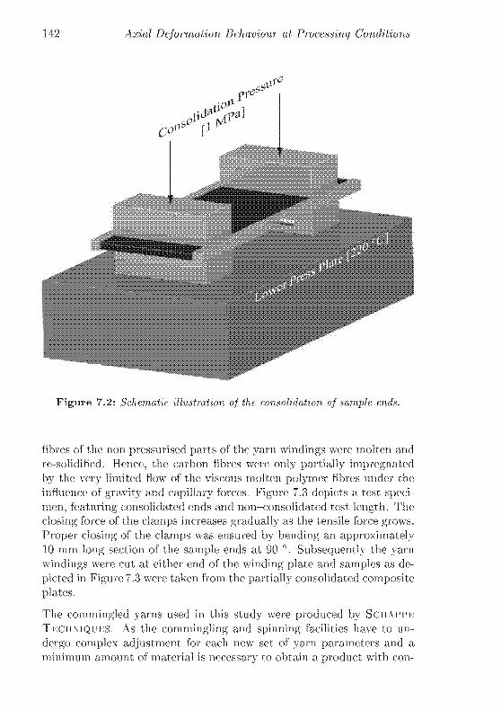
142 Axial Deformation Behaviour at Processing Conditions
Figure 7.2: Schematic illustration of the consolidation of sample ends.
fibres of the non pressurised parts of the yarn windings were molten and
re-solidified. Hence, the carbon fibres were only partially impregnated
by the very limited flow of the viscous molten polymer fibres under the
influence of gravity and capillary forces. Figure 7.3 depicts a test speci¬
men, featuring consolidated ends and non-consolidated test length. The
closing force of the clamps increases gradually as the tensile force grows.
Proper closing of the clamps was ensured by bending an approximately10 mm long section of the sample ends at 90 °. Subsequently the yarn
windings were cut at either end of the winding plate and samples as de¬
picted in Figure 7.3 were taken from the partially consolidated composite
plates.
The commingled yarns used in this study were produced by Sciiappk
Tkchmqi i:s. As the commingling and spinning facilities have to un¬
dergo complex adjustment for each new set of yarn parameters and a
minimum amount of material is necessary to obtain a product with con-
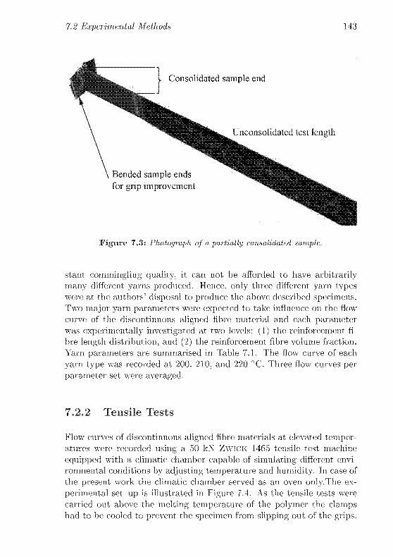
7.2 Experimental Methods 143
Figure 7.3: Photograph of a partially consolidated, sample.
stant commingling quality, it can not be afforded to have arbitrarily
many different yarns produced. Hence, only three different yarn types
were at the authors' disposal to produce the above described specimens.Two major yarn parameters were expected to take influence on the flow
curve of the discontinuous aligned fibre material and each parameter
was experimentally investigated at two levels: (1) the reinforcement fi¬
bre length distribution, and (2) the reinforcement fibre volume fraction.
Yarn parameters are summarised in Table 7.1. The flow curve of each
yarn type was recorded at 200, 210, and 220 °C. Three flow curves per
parameter set were averaged.
7.2.2 Tensile Tests
Flow curves of discontinuous aligned fibre materials at elevated temper¬
atures were recorded using a 50 kN ZwiCK 1465 tensile test machine
equipped with a climatic chamber capable of simulating different envi¬
ronmental conditions by adjusting temperature and humidity. In case of
the present work the climatic chamber served as an oven only.The ex¬
perimental set up is illustrated in Figure 7.4. As the tensile tests were
carried out above the melting temperature of the polymer the clampshad to be cooled to prevent the specimen from slipping out of the grips.

144 Axial Deformation Behaviour at Processing Conditions
Table 7.1: Yarn Parameters
Designation CF w-Fract.a CF w-Fract.6 mc
[%] [%]
CF50 64 50 standard
CF56 68 56 standard
CFs 64 50 short
"Weight fraction of carbon fibres
'Volume fraction of carbon fibres in the void free laminate
cFibre length distribution
The cooling system is depicted in Figure 7.5. To keep the tempera¬
ture gradient along the specimen caused by the clamp cooling small, the
cooling system needed to be adjusted to a moderate cooling level. The
coolant flow was controlled manually by means of a w7atcr flow meter
and the flow was set to 5 • 10~5 m3 s"1. To keep the experimental pro¬
gram manageable the deformation rate was kept constant throughoutthis study despite the fact that it might take influence on the flow be¬
haviour of aligned fibre filled viscous liquids. The drawing speed was set
to 1.67- lO^ms"1.
7.3 Flow Curve Modelling
The flow curve is expected to obey the Herschel-Bulkley model, which
adds an ideal Saint-Venant element to the damping element of the well
known Maxwell model (Figure 7.6). The visco-clastic behaviour of the
present system of aligned discontinuous carbon fibres partially embedded
in molten polymer can thus be separated into two stages:
I. the tensile stress increases until a maximum is reached and
II. stress relaxation according to the simple Maxwell model once
the adhesional stress capacity of the Saint Venant element is ex¬
hausted.
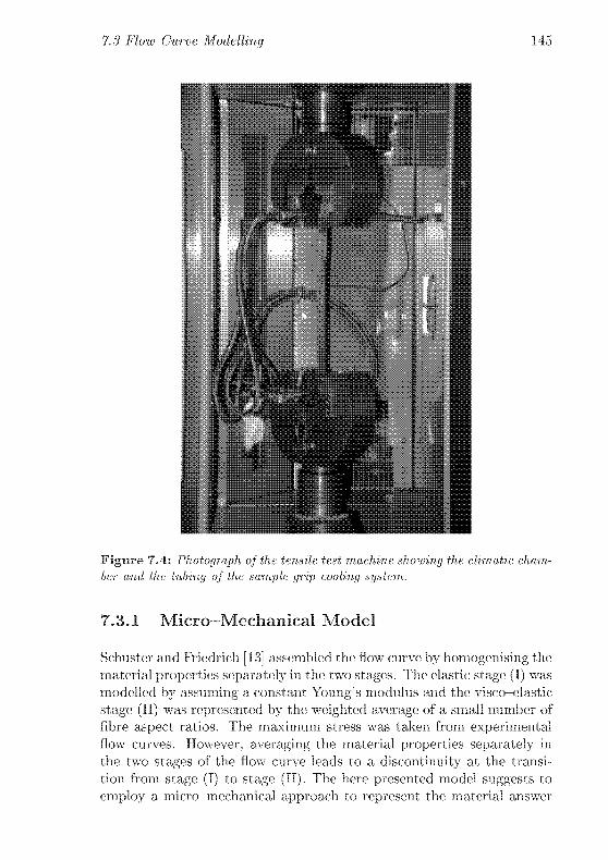
7.3 Flow Curve Modelling 145
Figure 7.4: Photograph of the tensile test machine showing the climatic cham¬
ber and, the tubing of the sample grip cooling system.
7.3.1 Micro-Mechanical Model
Schuster and Friedrich [13] assembled the flow curve by homogenising the
material properties separately in the two stages. The elastic stage (1) wasmodelled by assuming a constant Young's modulus and the visco—clastic
stage (II) was represented by the weighted average of a small number of
fibre aspect ratios. The maximum stress was taken from experimentalflow curves. However, averaging the material properties separately in
the two stages of the flow curve leads to a discontinuity at the transi¬
tion from stage (I) to stage (II). The here presented model suggests to
employ a micro mechanical approach to represent the material answer

146 Axial Deformation Behaviour at Processing Conditions
Ë^^xÈJfvM^^^^^^^^^^sllfL^^i,
f _^^fiSw IaMIMl»
ÉllÉ" ::::::::::::: "^^^^^^ ""*!|^^^^^^ ^1»m^^^H
pi = Al ' 1%"
ii)
KJ*"
j ,,_
Jtlfci«,,,
1*-.. .f**^*"'" "'v<
mfTTT""W,îïi" "'" '
Figure 7.5: Photograph of the upper chuck head with water cooled clamps.
Damping Element
Spring Element
al = Emel if <7<<7
<7TT = i?Feen if <7><T
-WM
<-= ?J£p
Saint \fenant E
(7
lement
Figure 7.6: Schematic illustration of the rheological model according to
Herschel-Bulkley.

7.3 Flow Curve Modelling 147
to externa] stresses along the fibre axis. A single fibre of length I and
radius rf interacts with its immediate neighbourhood (that is polymermelt and adjacent fibres) at a portion of its own length the relative
interaction length Ô. The stress strain behaviour of such a micro systemis assumed to obey the Herschel-Bulkley model and thus each considered
micro model with parameters £ and 6 will exhibit a characteristic flow-
curve with a linear clastic part and visco-clastic stress relaxation part.
The flow curve is thought to be the weighted sum of the total stress-
strain curve of single fibre models where for each micro-model different
values of £ and S are considered and to each pair of £ and <5 a certain
statistical probability is assigned. If such a micro model is exposed to an
external force field it will resist deformation, resulting in internal tensile
stress a. In fact, the evolution of the pulling force F per unit cell area
Au as would be observed in an imaginary tensile test of a micro model
is considered:
°-Xis] <7-'>
The unit cell contains one fibre. Its area .4U can be expressed as a func¬
tion of the average distance between neighbouring fibres—i.e. the fibre
spacing S, which itself is determined by the macroscopic fibre volume
fraction i/f of the composite:
S = 2nd— ("-2)V V{
where v is the maximum available fibre volume fraction at a given fi¬
bre packing geometry. Simple geometric evaluation of a quadratic or
hexagonal fibre packing array delivers the unit cell area in terms of fibre
spacing 5:
{S2(quadratic)
n(7-:i)
^fS2 (hexagonal)
Referring to Figure 7.7 it is obvious that the maximum available fibre
volume fraction at a given packing array is obtained by simply settingthe fibre spacing S equal to the fibre diameter 2 rf, namely:
— (quadratic)
(7-4)—= (hexagonal)
The maximum fibre volume fraction in case of a hexagonal array is equalto the maximum space filling of cylinders of equal diameters and it de¬
picts a theoretical limit, which cannot be achieved in practice. Hence,
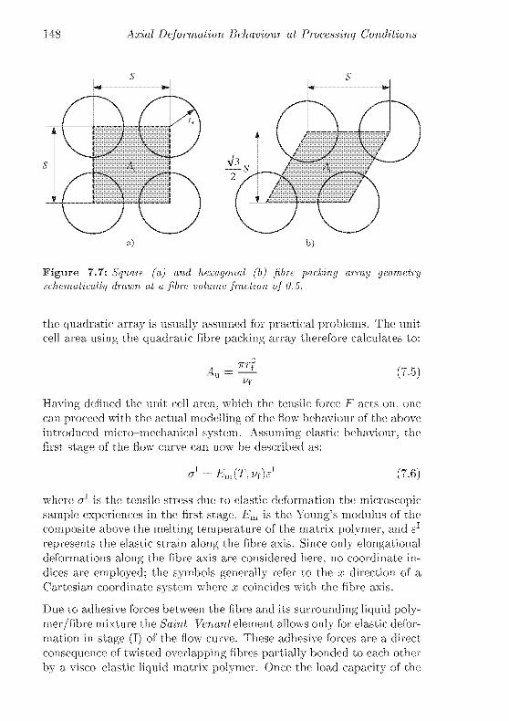
148 Axial Deformation Behaviour at Processing Conditions
Figure 7.7: Square fa) and hexagonal (b) fibre packing array geometry
schematically drawn at a fibre volume fraction of 0.5.
the quadratic array is usually assumed for practical problems. The unit
cell area using the quadratic fibre packing array therefore calculates to:
AuVf
(7.5)
Having defined the unit cell area, which the tensile force F acts on, one
can proceed with the actual modelling of the flow behaviour of the above
introduced micro-mechanical system. Assuming elastic behaviour, the
first stage of the flow curve can now be described as:
a1 = Em(T>f)tJ (7.6)
where a1 is the tensile stress due to clastic deformation the microscopic
sample experiences in the first stage, Em is the Young's modulus of the
composite above the melting temperature of the matrix polymer, and el
represents the elastic strain along the fibre axis. Since only elongationaldeformations along the fibre axis are considered here, no coordinate in¬
dices are employed; the symbols generally refer to the x direction of a
Cartesian coordinate system where x coincides with the fibre axis.
Due to adhesive forces between the fibre and its surrounding liquid poly¬
mer/fibre mixture the Saint Venant element allows only for elastic defor¬
mation in stage (I) of the flow curve. These adhesive forces are a direct
consequence of twisted overlapping fibres partially bonded to each other
by a visco elastic liquid matrix polymer. Once the load capacity of the

7.3 Flow Curve Modelling 149
Saint-Venant element is exhausted the maximum stress is reached and
stress relaxation sets on.
It is clear that the above discussed discontinuous transition from stage (1)to stage (II) (i.e. at a1 = a) also has to occur in the micro mechanical
model (or in a multi fibre model where only one fibre and interaction
length is considered). In stage (IT) the Maxwell model implies that the
total strain e equals the sum of deformations in the spring element and
the damping element, i.e. the sum of elastic and plastic deformation. e0
andcp, respectively:
e = ee + fp (7.7)
and accordingly in terms of strain rate:
...
vU à11e = ee +ep= + ———- 7.8)
iF(I,i/r) 7i(I,e, v{)
where Ep is an elastic constant and rj is the molten fibre composite's vis¬
cosity. At constant strain rate the general solution of such a differential
equation is:
cru = Gexp(~^)+r,é (7.9)
where C is a constant to be determined by considering boundary condi¬
tions. Introducing ta- as the time elapsed until the maximum stress â is
reached we obtain:
.n
a1 if t < tà
<t"=< ,. .x/ EF(t-U)\
,. .,.. . (7.10)
(a - T]s) cxp I^—2^ J + t]£ if t > ta
Although stress relaxation effects arc generally expressed in terms of
time the present authors suggest to use the deformation velocity as an
expression of passed experimental time rather than the—in fact from
the experiment entirely detached—time itself. Assembling stresses in
stage (I) and (II) and plotting them against the strain delivers the flow
curve of the micro-model, which is in fact equivalent to the flow curve
of a multi fibre material with a constant fibre length and a constant
length of interaction. Such a flow curve is illustrated in Figure 7.8. The
selected parameter values as given in Figure 7.8 represent the most prob¬able numbers for the predictand of the fibre length in case of standard
length distribution.
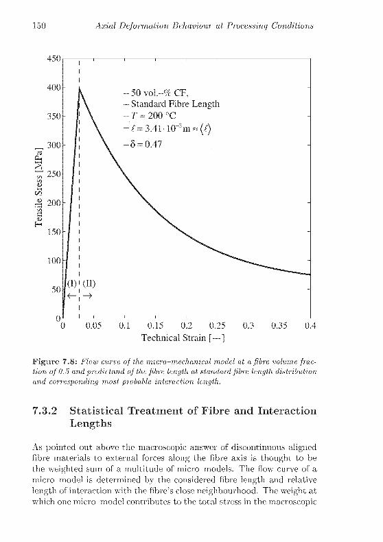
150 Axial Deformation Behaviour at Processing Conditions
450
400
350
300
250
150
100
50(1)
- 50 vol.-% CF,- Standard Fibre Length- T = 200 °C
-^ = 3.41-Hr2m = {4-5 = 0.47
(II)
0.05 0.1 0.15 0.2 0.25
Technical Strain [—]
0.3 0.35 0.4
Figure 7.8: Flow curve of the micro-mechanical model at a fibre volume frac¬tion of 0.5 and predictand of the fibre length at standard fibre length distribution
and corresponding most probable interaction length.
7.3.2 Statistical Treatment of Fibre and Interaction
Lengths
As pointed out above the macroscopic answer of discontinuous alignedfibre materials to external forces along the fibre axis is thought to be
the weighted sum of a multitude of micro models. The flow curve of a
micro model is determined by the considered fibre length and relative
length of interaction with the fibre's close neighbourhood. The weight at
which one micro model contributes to the total stress in the macroscopic
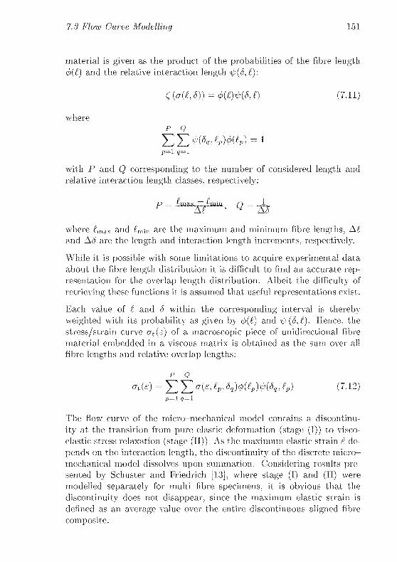
7.3 Flow Curve Modelling 151
material is given as the product of the probabilities of the fibre length
(b(£) and the relative interaction length ip(S,(f):
Ç(a({,8))=cp({)ii8,t) (7.11)
where
p Q
p-\ q-\
with P and Q corresponding to the number of considered length and
relative interaction length classes, respectively:
where £max and (m-m are the maximum and minimum fibre lengths, A£
and AS are the length and interaction length increments, respectively.
While it is possible with some limitations to acquire experimental data
about the fibre length distribution it is difficult to find an accurate rep¬
resentation for the overlap length distribution. Albeit the difficulty of
retrieving these functions it is assumed that useful representations exist.
Each value of £ and 6 within the corresponding interval is thereby
weighted with its probability as given by <j)(£) and ijj(6,(). Hence, the
stress/strain curve o~i(e) of a macroscopic piece of unidirectional fibre
material embedded in a viscous matrix is obtained as the sum over all
fibre lengths and relative overlap lengths:
p Q
a^ = EE^MpAWpK-ow (7-12)p-l q-\
The flow curve of the micro-mechanical model contains a discontinu¬
ity at the transition from pure elastic deformation (stage (I)) to visco-
elastic stress relaxation (stage (11)). As the maximum clastic strain s de¬
pends on the interaction length, the discontinuity of the discrete micro-
mechanical model dissolves upon summation. Considering results pre¬
sented by Schuster and Friedrich [13]. where stage (I) and (IT) were
modelled separately for multi fibre specimens, it is obvious that the
discontinuity does not disappear, since the maximum elastic strain is
defined as an average value over the entire discontinuous aligned fibre
composite.
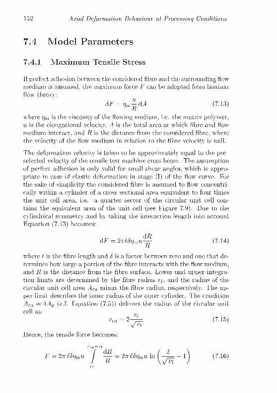
152 Axial Deformation Behaviour at Processing Conditions
7.4 Model Parameters
7.4.1 Maximum Tensile Stress
If perfect adhesion between the considered fibre and the surrounding flow
medium is assumed, the maximum force E can be adopted from laminar
flow theory:
dF = rim^-dA (7.13)R
where i]m is the viscosity of the flowing medium, i.e. the matrix polymer,u is the elongational velocity, A is the total area at which fibre and flow
medium interact, and R is the distance from the considered fibre, where
the velocity of the flow medium in relation to the fibre velocity is null.
The deformation velocity is taken to be approximately equal to the pre
selected velocity of the tensile test machine cross beam. The assumptionof perfect adhesion is only valid for small shear angles, which is appro¬
priate in case of elastic deformation in stage (I) of the flow- curve. For
the sake of simplicity the considered fibre is assumed to flow concentri¬
cally within a cylinder of a cross sectional area equivalent to four times
the unit cell area, i.e. a quarter sector of the circular unit cell con¬
tains the equivalent area of the unit cell (sec Figure 7.9). Due to the
cylindrical symmetry and by taking the interaction length into account
Equation (7.13) becomes:
dT = 2Ti£8ikau^r (7.14)R
where / is the fibre length and S is a factor between zero and one that de¬
termines how large a portion of the fibre interacts with the flow medium,and R is the distance from the fibre surface. Lower und upper integra¬tion limits are determined by the fibre radius rf, and the radius of the
circular unit cell area Acu minus the fibre radius, respectively. The up¬
per limit describes the inner radius of the outer cylinder. The condition
Acu = AAU (cf. Equation (7.5)) delivers the radius of the circular unit
cell as:
rcu=2-^= (7.15)\/T{
Hence, the tensile force becomes:
r,-u-rr
F = 2irtST]mu f ^ = 2ntÖTfau )n (y= - l\ (7.16)
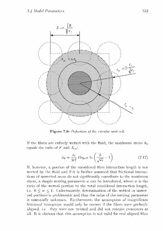
1.4 Model Parameters 153
Figure 7.9: Definition of the circular unit cell.
If the fibres are entirely wetted with the fluid, the maximum stress &q
equals the ratio of F and Acu:
0o f0î]mUhll 1 (7.17)
If, however, a portion of the considered fibre interaction length is not
wetted by the fluid and if it is further assumed that frictional interac¬
tions of uiiwetted areas do not significantly contribute to the maximum
stress, a simple wetting parameter w can be introduced, where w is the
ratio of the wetted portion to the total considered interaction length,i.e. 0 < w < 1. Unfortunately, determination of the wetted or unwct-
ted portions is problematic and thus the value of the wetting parameter
is essentially unknown. Furthermore, the assumption of insignificantfrictional interaction would only be correct if the fibres were perfectly
aligned, i.e. they were not twisted and did not contain crossovers at
all. It is obvious that this assumption is not valid for real aligned fibre

154 Axial Deformation Behaviour at Processing Conditions
materials. The degree of fibre twist and crossover is again unknown and
cannot easily be determined, so that an arbitrary twist factor 0 > 1 has
to be assumed. Hence, the theoretic maximum tensile stress «tq has to
be multiplied with the correcting factors w and 9 to become:
a = ao0w(£) (7.18)
It is intuitively acceptable that the wetting parameter depends on the
considered fibre length in such a way that the probability of full wet¬
ting decreases with growing fibre length. The portion of wetted area is
thought to depend on fibre volume fraction and quality of commingling,which itself depends on a number of parameters as pointed out in de¬
tail in [14]. In a first step the average number of carbon fibres (rVf) to
be wetted by one polymer fibre of length {£m) and radius rm has to be
calculated:
/ArXr2{£m)vf
<Af)=r?<00-^)(7"19)
where (I) = Y2 Cp©(£p) is the average carbon fibre length, (£m) approxi¬
mately equals 70 mm and the carbon and polymer fibre radii r{ and rm
are 3.5-106 m and 1.15-10"5 m, respectively [14]. From Equation (7.19)an estimated value of the initially wetted fibre fraction can be given as
the surface fraction (am) of polymer fibres:
\Qn») = ir \ i ii)\i-\t\ (1.3A)rm{£m) + rf{f){J\f)
Again referring to [14] it is found that the polymer fibres exhibit a rel¬
atively narrow fibre length distribution, which justifies to employ the
average value as a representative length of the polymer fibres. Takingvariable carbon fibre length into account, the wetting parameter is thus
assumed as:
w(() = (am)^ (7.21)
The twist factor 0 is related to the number of fibre crossovers per fi¬
bre unit length. Since there is no reliable way to determine its value
experimentally, it remains in the model as a scaling factor.
7.4.2 Viscosity of Fibre Filled Liquids
According to Pipes et al. [8] the elongational viscosity i] of a fibre filledt
2rtresin the fibres having constant aspect ratio J~ and the relative length

14 Model Parameters 155
of interaction S being ^ is:
where r/m is the resin viscosity and Ff is the normalised fibre volume frac¬
tion, defined as the ratio of present to maximum available fibre volume
fraction as discussed above:
nV{ = ~r
v
For the here investigated poly(laurolactam) it was found that the resin
viscosity depends on temperature according to Arrhenius and it was
observed that, in case of low viscosity poly(laurolactam) melts, no con¬
siderable shear thinning occurs at deformation rates ranging from 10 to
1000 s"1, i.e. the polymer melt behaves like a Newtonian fluid [15]:
Vm = J7mo exp I ^~ j (7.23)
with 57,1,0 = 1.59 • 10~~4Pas being the theoretic resin viscosity at infinite
temperature, and the ratio of the activation energy for viscous flow to
the universal gas constant Ej\/R =7073 K [16].If the interaction length is a constant but arbitrary portion of the fibre
length, Equation (7.22) becomes [9]:
r,{l,6) = 2rhnvf(J^ S(\-S)(j^=^ (7.24)
Although the case has been made for variable fibre and overlap lengths,the variations of both being governed by the same probability func¬
tion [9], this approach is not further explored here since the presentedmicro model only describes interaction of one single fibre with its imme¬
diate environment, i.e. in the micro model fibre and interaction lengthsare constant. Statistical aspects, however, are vitally important for the
presented modelling approach and they will be discussed in the next
section.
It was mentioned above that incomplete fibre wetting has to be expected.The thus reduced effective interaction length will be taken into account
by adjustment of the respective probability ip(fp,ôq).

156 Axial Deformation Behaviour at Processing Conditions
7.4.3 Elastic Moduli
Rather than seeking a direct way to derive the elastic constant in stage (I)of the flow curve, we suggest to calculate it via Hooke's law:
fim = % = ~ (7-25)eL e
This approach is motivated due to the assumption that the strain at
maximum stress ê depends on yarn architecture only (i.e. fibre lengthdistribution, reinforcement fibre fraction, and fibre twist), and. hence, it
is expected to be constant for a given yarn. Considering experimentalresults the validity of this assumption is evident (see Chapter 7.5).
To get hold of the strain at maximum tensile stress ê the propertiesof the micro-mechanical model are homogenised over a normalised and
thus dimensionless imaginary test volume defined by a cylinder of radius
r* = Tcu/rf = 2/yTvf and height h* = öi/L, where L is an arbitrary
scaling length, e.g. here it might equal the minimum fibre length ^min-
We bear in mind that the sole purpose of the normalisation is to obtain
an imaginary test volume, which exhibits an aspect ratio reasonably close
to unity for all considered interaction lengths. This test volume is now
treated as if it consisted of a monolithic material of axial viscosity rj. If
a tensile force acted along the cylinder axis, the circular base and top
faces would deform to cones with the cone angle being equivalent to the
imaginary shear angle ->i, namely:
eh* e£8JTrt
tan7l = —= —*— (7.26)r ztiniii
As the maximum tensile force increases with growing interaction length,the deformation resistance of the imaginary cylinder also increases pro¬
portionally. The imaginary shear angle depends on the aspect ratio of
the test volume but stays constant for all values of £ and 5. Hence, the
elastic strain at maximum tensile stress times the interaction length has
to be constant as well and the elastic constant therefore becomes:
2/min tan ">i
Note that the imaginary shear angle is only thought to envision that the
product of maximum elastic strain and interaction length is constant. It
does not claim to have any physical significance.
The elastic constant in stage (I) of the flow curve was determined via
Hooke's law and incorporated knowledge of the maximum tensile stress.

14 Model Parameters 157
which was derived using laminar flow theory by assuming perfect adhe¬
sion between fibres and viscous matrix. In case of the elastic constant in
the visco elastic part of the flow curve, the fibre/matrix interaction is.
however, governed by hydrodynamic friction rather than adhesion. Ob¬
viously, the ratio of the elastic constant in stage (I) to that in stage (11)must be equal to the ratio of elastic stresses in stage (I) and (11) :
liip o~p fp
where F is the maximum force acting on the circular unit cell area and
the subscript F refers to the frictional nature of the parameters in the
denominator.
The problem of determining the frictional elastic constant is now shifted
to a problem of calculating the frictional force Fp, which is in fact equallydifficult to solve but can be dealt with more intuitively. The frictional
force Fp equals according to Amonton's law the product of normal force
Tn and the friction coefficient pp. Under tensile loading a given fibre
bundle contracts due to the fibres not being perfectly aligned but twisted
slightly. The applied tensile force therefore causes the angle between
slightly misaligned fibres and the force direction to decrease. The liq¬uid polymer resists this contraction and thus provokes the normal force
to evolve. If we now consider again the fibre sliding within a hollow
cylinder of inner radius rcu the inner wall of which is an equivalent to
the surfaces of the neighbouring fibres—we meet a situation where the
film of polymer melt between the fibre and inner cylinder wall serves
as a lubricant. The friction coefficient for lubricated friction pm is in
the order of 10~"3 to 10-2 at the presence of a liquid lubricant [17]. In
the present situation, however, only part of the fibre surface is covered
with polymer melt acting as lubricant. Air serves as lubricant at the
unwetted portions of the fibre and the friction coefficient with air as lu¬
bricant /i,\i,. is in the order of 10~4 [17]. As the coefficient of friction
at the presence of a lubricant depends on the lubricants viscosity it can
be expected to decrease slightly with increasing temperature. The total
friction coefficient pp is therefore given as:
pv = /im(r/m)w(£) + A*Air(l - w(t)) (7.29)
with the dependence of /tm on viscosity assumed to be linear.
The normal force /Aj can again be calculated by means of laminar flow-
theory, where a fluid flows transversely around a cylinder of infinite
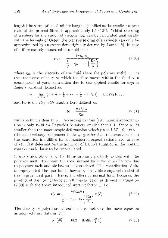
158 Axial Deformation Behaviour at Processing Conditions
length (the assumption of infinite length is justified as the smallest aspect
ratio of the present fibres is approximately 1.5 103). Whilst the dragof a sphere for the region of viscous flow can be calculated analyticallywith the formula of Oseen, the transverse drag of a cylinder can only be
approximated by an expression originally derived by Lamb [18]. In case
of a fibre entirely immersed in a fluid it is:
_
Anî]mu±Ho~l 7ï^ ('-30)
2-7E-ln
where r)m is the viscosity of the fluid (here the polymer melt), n \ is
the transverse velocity at which the fibre moves within the fluid as a
consequence of yarn contraction due to the applied tensile force,^e is
Euler's constant defined as:
TR = lim (l + i + 1 + ... + I- ln(n)) = 0.577216...,
and Re is the Reynolds number here defined as:
Re=^i (7.31)
with the fluid's density pm. According to Finn [19]. Lamb's approxima¬tion is only valid for Reynolds Numbers smaller than 0.1. Since u. is
smaller than the macroscopic deformation velocity n = 1.67- 10"-2ms""1
(the axial velocity component is always greater than the transverse one)this condition is fulfilled for all considered aspect ratios here. In case
of very fast deformation the accuracy of Lamb's equation in the present
context would have to be reconsidered.
It was stated above that the fibres are only partially wetted with the
polymer melt. To obtain the total normal force the sum of forces due
to polymer melt and air has to be considered. The contribution of the
unimpregnated fibre portion is, however, negligible compared to that of
the impregnated part. Hence, the effective normal force becomes the
product of the normal force at full impregnation as defined in Equation
(7.30) with the above introduced wetting factor w, i.e.:
,. 4-irr]mU[
1 /Re
2~7E~lnfT
w(£) (7.32)
The density of poly(laurolactam) melt pm satisfies the linear equation
as adopted from data in [20]:
Pm[„$] = 1002 - 0.585T[°C] (7.33)
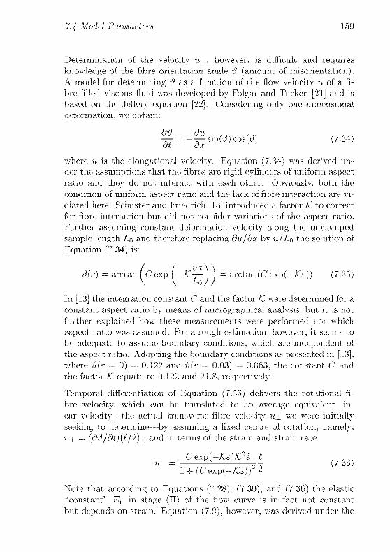
14 Model Parameters 159
Determination of the velocity it \ , however, is difficult and requires
knowledge of the fibre orientation angle it (amount of misorientation).A model for determining ê as a function of the flow velocity m of a fi¬
bre filled viscous fluid was developed by Folgar and Tucker [21] and is
based on the Jcffery equation [22]. Considering only one dimensional
deformation, we obtain:
^ = -|^sin(ö)coSW (7.34)
where u is the elongational velocity. Equation (7.34) was derived un¬
der the assumptions that the fibres arc rigid cylinders of uniform aspect
ratio and they do not interact with each other. Obviously, both the
condition of uniform aspect ratio and the lack of fibre interaction are vi¬
olated here. Schuster and Friedrich [13] introduced a factor K. to correct
for fibre interaction but did not consider variations of the aspect ratio.
Further assuming constant deformation velocity along the undamped
sample length L0 and therefore replacing dn/dx by u/Ln the solution of
Equation (7.34) is:
d(e) = arctan I Cexp I —K'.-j- ) ) = arctan (Cexp(—K,s)) (7.35)
In [13] the integration constant C and the factor A were determined for a
constant aspect ratio by means of micrographical analysis, but it is not
further explained how these measurements were performed nor which
aspect ratio was assumed. For a rough estimation, however, it seems to
be adequate to assume boundary conditions, which are independent of
the aspect ratio. Adopting the boundary conditions as presented in [13],where £)(e = 0) = 0.122 and £)(s = 0.03) = 0.063. the constant C and
the factor K. equate to 0.122 and 21.8, respectively.
Temporal differentiation of Equation (7.35) delivers the rotational fi¬
bre velocity, which can be translated to an average equivalent lin¬
ear velocity the actual transverse fibre velocity u i we were initially
seeking to determine by assuming a fixed centre of rotation, namely:
v± = (dd/dt)(£/2) ,and in terms of the strain and strain rate:
Cexp(-£e)/C2e £
l + (C7cxp(-/Cs))22Ml =
. ;—ZTTT2ÏÏ (i.36)
Note that according to Equations (7.28), (7.30), and (7.36) the elastic
"constant" Ep in stage (II) of the flow curve is in fact not constant
but depends on strain. Equation (7.9), however, was derived under the
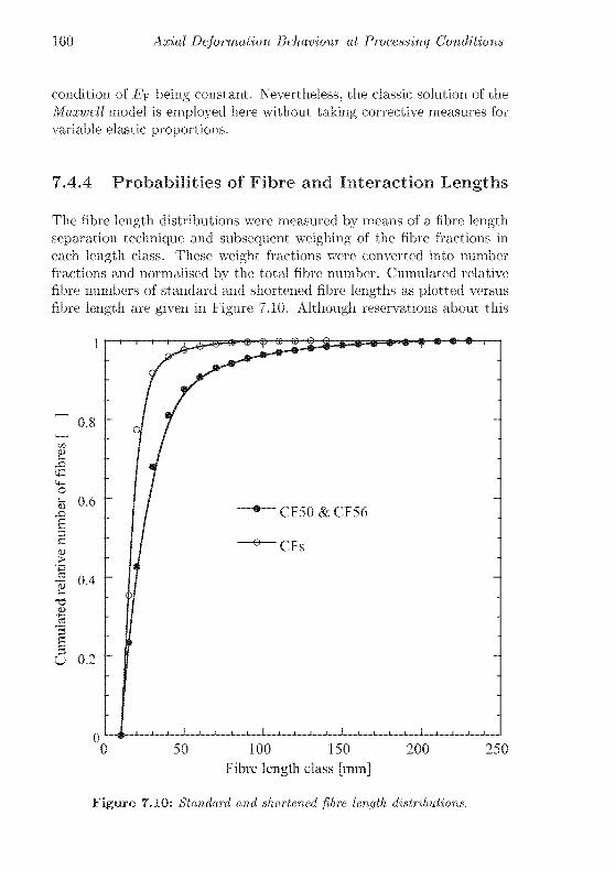
160 Axial Deformation Behaviour at Processing Conditions
condition of Ep being constant. Nevertheless, the classic solution of the
Maxwell model is employed here without taking corrective measures for
variable elastic proportions.
7.4.4 Probabilities of Fibre and Interaction Lengths
The fibre length distributions were measured by means of a fibre length
separation technique and subsequent weighing of the fibre fractions in
each length class. These weight fractions were converted into number
fractions and normalised by the total fibre number. Cumulated relative
fibre numbers of standard and shortened fibre lengths as plotted versus
fibre length are given in Figure 7.10. Although reservations about this
a
X>
>•-a
-a
U 0.2
100 150
Fibre length class [mm]
250
Figure 7.10: Standard and shortened fibre length distributions.

14 Model Parameters 161
fibre length measurement method have been made [13], the fibre lengthdistributions as depicted in Figure 7.10 were nevertheless employed here
to express the fibre length probability <f>(£).
Experimental determination of the interaction length, however, is ex¬
tremely difficult. The authors could not think of a practical method
capable of delivering such data. Therefore, it has to be relied on reason¬
able guesses about the actual shape of the probability function of the
interaction length. It will be assumed here that the relative interaction
length somehow obeys a modified normal distribution. Intuitively it is
easy to accept that the probability to find a fibre of length (, which
interacts with its neighbourhood at certain portion «5 of its own length,
depends on the fibre length. This dependence is implemented by intro¬
ducing a term which shifts the peak of the normal distribution between
<5min = 0 and <ïmax = 1 (be. no interaction and interaction along the
entire fibre length, respectively), so that the probability of <5max = 1
decreases to null with the fibre length approaching its maximum value:
'C {S, f) = cxp (--±- (s + w(£) - (1 - Tf)2) (7-37)
where the factor k and the exponent ß are set somewhat arbitrarilydue to the lack of knowledge about the shape of the interaction lengthdistribution. £* is the relative fibre length defined as:
£* =£ ~^"';n (7.38)
In Figure 7.11 the viscosity contribution of each micro model in case of
(a) standard and (b) shortened fibre length distribution (i.e. the productof Equation (7.24) with the experimentally obtained fibre length distri¬
bution as shown in Figure 7.10 and the interaction length probability as
presented in Equation (7.37)) is plotted versus the relative fibre length£* and the relative interaction length 8. The fibre length and relative
interaction length increment is \£ = (fmax — ^min)/100 and \5 = 0.01,
respectively, resulting in 104 evaluated combinations of / and 8. Fig¬ure 7.11 illustrates both the statistical aspects discussed above and the
strong influence of the fibre aspect ratio on the evolution of the viscos¬
ity. Comparison of viscosity contribution of the two different fibre lengthdistributions particularly emphasises the importance of fibre length.

162 Axial Deformation Behaviour at Processing Conditions
a)
b)
Figure 7.11: Viscosity contribution of each pan of fibre length and lelative
interaction length m case of (a) standard and (b) shortened fibre length distri¬
bution

15 Results 163
7.5 Results
Experimentally determined and corresponding simulated flow curves at
different temperature levels are presented in Figure 7.12, 7.13, and 7.14.
350
300
250
200
1.50a
H
100
50
50\ol-%CF,Standard Fibre Length
200 °C
210 °C
220 °C
\
A \
0 05 0 1 0 15 0 2 0 25
Technical Strain [—]
03 0 35 04
Figure 7.12: Measured and calculated flow curves of yam with 50 volume-
ear bon fibies at standard fibre length distribution (CF50).
Experimental flow curves represent average values from three to five mea¬
surements and en or bars are plotted along with the average data. Due
to the vast number of data points the measured flow curves appear as
scatter bands illustiated in different shades of grey for respective experi¬mental temperatures. Best agreement between measured and simulated
flow curves was achieved with k and 3 equal to 1/2 and 3, respectively.

164 Axial Deformation Behaviour at Processing Conditions
lOU
- - 200 °C
160-- 210 °C
-
,~\ 220 °C
,x 56 vol.-% CF,
140 -
,* \ Standard Fibre Length*\
.' \
,_
120 .
l \
rräTi s
& i' >. \^ Ii, \ **
XT 100 - 'ML ">"
JMMfc. \ v
2 :^^^^x.
snsileS
00o
PlfefcL"--H If ^MBBBfch»>^
60 f ^^^^fciL^ ^-^I ^^^fc
--. -->.
f ^^^_~~_40
1 ^——:
20 I0.05 0.1 0.15 0.2 0.25 0.3
Technical Strain [m/mj
0.35 0.4
Figure 7.13: Measured and calculated flow curves of yarn with 56 volume-%
carbon fibres at standard fibre length distribution (CF56).
These are also the numbers used in Figure 7.11. Numerical values of
the twist factor 6 and the shear angle -?! as employed for the flow curve
simulations are listed in Table 7.2. As expected, comparison of exper¬
imental flow curves and simulation results delivers a linear relationshipbetween polymer viscosity and friction coefficient pm with the polymermelt acting as lubricant. The friction coefficient is found to obey:
M,n=4.0-10_V[Pas]+4.9- 10" (7.39)
Figure 7.15 shows simulation results at 220 °C and various fibre lengthdistributions. The minimum fibre length, however, cannot be changed
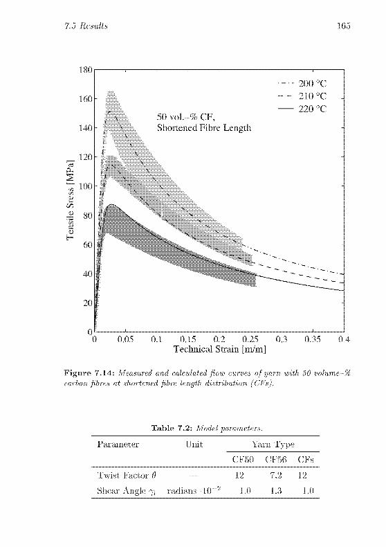
1.5 Results 165
180
160
140
120
100
60
40
20
50 voi.-% CF,
Shortened Fibre Length
200 °C
210 °C
220 °C
O10 0.05 0.1 0.15 0.2 0.25 0.3 0.35 0.4
Technical Strain [m/m]
Figure 7.14: Measured and calculated flow curves of yarn with 50 volume %
carbon fibres at shortened fibre length distribution (CFs).
Table 7.2: Model parameters.
Parameter Unit Yarn Type
CF50 CF56 CFs
Twist Factor 0 12
Shear Angle 7, radians-10""2 1.0
7.2 12
1.3 1.0

166 Axial Deformation Behaviour at Processing Conditions
1UU
— ô=1.0
- - è=2.090 -
rx Variation of Fibre Length
,' \ £p = (nvil+bpA£
- è=0.5"
80 - l xr . .
-i-
• \ £ -Üi/-\
% p =A m<LX mm 1
701/ \ s
M-
1/ \ x
CS 1 \. ^
if ^v •*
Ü 60"'I - \.Nx
_
V3
«
0)
50
J* --../^^_
r=i
S 40 -J' '"*"*"*'->—^"^^^-^w-
D Ii ""', '"«"
."''"""""
H
ii^^
30 -
20 -
10
A
-
0 0.05 0.1 0.15 0.2 0.25 0.3 0.35 0.4
Technical Strain [m/m]
Figure 7.15: Simulated flow curves at scaled fibre length distribution of CFs
yarn.
as it is constant due to the stretch braking process. To maintain the
same minimum fibre length for all flow curves in Figure 7.15. the fibre
length distribution of CFs yarn is therefore scaled by multiplication of the
length increment A£ with a constant factor b. The solid line represents
the flow- curve of the unchanged CFs fibre length distribution.
1.6 Discussion 167
7.6 Discussion
Experimental results show relatively large scattering. This is attributed
to slightly different thermal gradients along the samples during the ten¬
sile tests. To prevent the sample from slipping out of the clamps it has
to be assured that the sample ends do not reach melting temperature
and, hence, a thermal gradient cannot be avoided. Although it was tried
to maintain the flow rate of coolant constant, small flow rate variations
due to fluctuations in the water supply system and stability of the preset
valve position bave to be expected. Additionally, the statistical nature of
yarn parameters is also bound to result in deviations of experimental ob¬
servations. Nevertheless, the good general agreement between the above
presented model and experimental flow curves suggests validity of the
selected micro mechanical simulation approach. Due to the complexityof the presented material system itself—featuring statistical reinforce¬
ment fibre length distribution and iiihomogeiicous blending—and due to
the incomplete fibre wetting, however, derivation of the maximum ten¬
sile stress and also the maximum clastic strain requires knowledge of the
shape of a measured reference flow7 curve.
Intuitively, one would assume existence of a simple relationship between
fibre length, fibre volume fraction, and the somewhat arbitrarily intro¬
duced twist factor 6. In case of both standard and shortened fibre lengthdistribution at a fibre volume fraction of 0.5, 6 is found to be 12, whereas
in case of standard fibre length distribution at V{ = 0.56 it equals 7.2.
To derive the wetting parameter, homogeneous blending of polymer and
reinforcement fibres was assumed. It was. however, reported that rel¬
atively large agglomerations of reinforcement fibres may occur [16, 23].According to [16], better blending is found in the yarn with shortened
fibre length distribution (CFs) among the yarns with 50 % fibre vol¬
ume fraction (CF50 fr CFs), and most iiihomogciieous blending qualitywas observed in case of the yarn featuring 56 % reinforcement fibre vol¬
ume fraction (CF56). The wetting parameter probably overestimates
the actual wetted fibre portion if the fibre volume fraction is increased,
and, hence, a smaller value of 0 has to be chosen to achieve good agree¬
ment between measured and calculated maximum tensile stress. With
decreasing fibre length on the other hand, one might also expect the
twist factor to decrease. This is, however, not observed here, which
again, has to be attributed to the wetting parameter. Fairly large over-
estimation of the wetted fibre portion due to inhomogeneous blendingis expected for all considered yarns but the accuracy of the predicted

168 Axial Deformation Behaviour at Processing Conditions
wetted area increases in the order w(CF56) < w(CF50) < iu(CFs).Defining the error of the wetting parameter as Aw it is thus obvious
that Aw(CF50) > Aiu(CFs). The maximum stress would then have to
be expressed as à = ôo (w — Aw) 9. This required an increase of 6 to
achieve agreement between calculated and measured tensile stress. Due
to Au;(CF50) > Aw(CFs) the increase would be more articulate in case
of CF50 compared to CFs. In other words, the error variation of the
wetting parameter due to inhomogencous blending compensates for the
twist factor, resulting in approximately equal values of the twist factors
for the CF50 and CFs yarns. The equality, however, must be considered
to be purely coincidental. Exactly the same argumentation is valid for
the shear angle 7.
Where calculated and measured flow curves agree well in case of CF56
and CFs yarns, the predicted peak curvature is wider than that of mea¬
sured flow curves in case of the CF50 yarn. This may be attributed
to inaccurate representation of the fibre length distribution. As alreadymentioned above, reservations about the measurement method to obtain
fibre length distributions have been made [13]. The same fibre lengthdistribution was assumed for CF56 and CF50 yarns. It is, however, imag¬inable that the fibre length distribution is slightly altered by the yarn
spinning, and this alteration might be influenced by the reinforcement
fibre content. A general tendency towards fibre shortening as a result
of increasing fibre interaction during spinning might be expected if the
reinforcement fibre content is increased.
For thermoforming purposes it is important to know the maximum ex¬
pectable force, which will act on the blank holder during moulding. The
here presented results show7 the dependence of both the maximum yarn
stress and the shape of the flow curve on yarn parameters and thermo¬
forming temperature. Increasing fibre length causes the maximum stress
and the viscosity according to Equation (7.24) to increase as well. The
influence of reinforcement fibre fraction on the other hand does not agree
with intuitive expectation and the here observed decrease with growingfibre fraction can only be attributed to incomplete state of consolidation
as already pointed out above. It is therefore illustrative to simulate flow
curves at different degrees of consolidation (i.e. by varying the w7etting
parameter) (Figure 7.16). and to consider different reinforcement fibre
fractions in case of complete impregnation (Figure 7.17). In Figure 7.16
the wetting parameter as calculated according to Equation (7.21) is mul¬
tiplied for each fibre length with a constant factor (i.e. 2 and 10 in the
presented example) as long as the product of this factor and the wet-
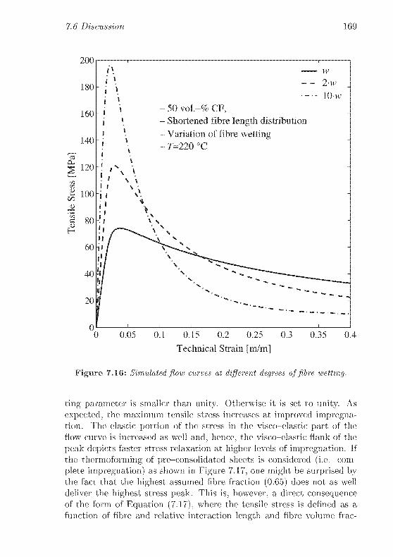
1.6 Discussion 169
200
180
160
140
§ 120
JlOO
1 80
60
40
20
0l
- - 2-w
- 10-w
- 50 vol-% CF,
- Shortened fibre length distribution
- Variation of fibre wetting- 7=220°C
N S
V.
\ s
0 0.05 0.1 0.15 0.2 0.25 0.3 0.35 0.4
Technical Strain [m/m]
Figure 7.16: Simulated flow curves at different degrees of fibre wetting.
ting parameter is smaller than unity. Otherwise it is set to unity. As
expected, the maximum tensile stress increases at improved impregna¬tion. The elastic portion of the stress in the visco-elastic part of the
flow7 curve is increased as well and, hence, the visco-elastic flank of the
peak depicts faster stress relaxation at higher levels of impregnation. If
the thermoforming of pre-consolidatcd sheets is considered (i.e. com¬
plete impregnation) as shown in Figure 7.17. one might be surprised bythe fact that the highest assumed fibre fraction (0.65) does not as well
deliver the highest stress peak. This is. however, a direct consequence
of the form of Equation (7.17). where the tensile stress is defined as a
function of fibre and relative interaction length and fibre volume frac-
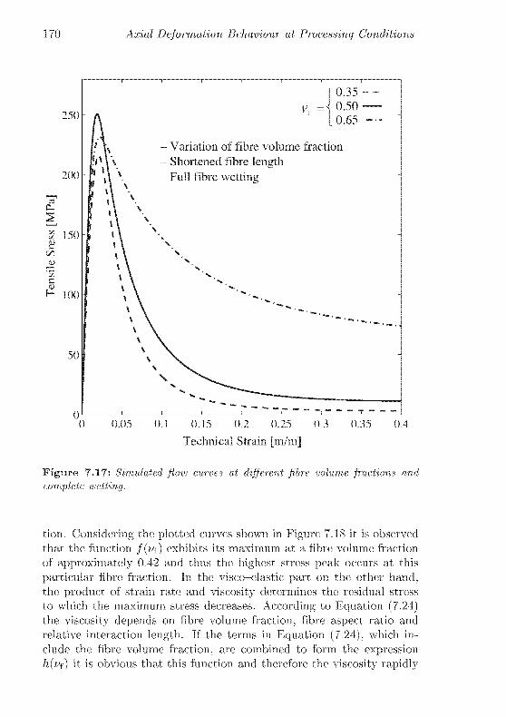
170 Axial Deformation Behaviour at Processing Conditions
250
200
ci
Cl,
150
H 100
50
0
- Variation of fibre volume fraction
- Shortened fibre length- Full fibre wetting
0 0.05 0.1 0.15 0.2 0.25 0.3 0.35 0.4
Technical Strain [m/mJ
Figure 7.17: Simulated flow curves at different fibre volume fractions and
complete wetting.
tion. Considering the plotted curves shown in Figure 7.18 it is observed
that the function f(vf) exhibits its maximum at a fibre volume fraction
of approximately 0.42 and thus the highest stress peak occurs at this
particular fibre fraction. In the visco-elastic part on the other hand,the product of strain rate and viscosity determines the residual stress
to which the maximum stress decreases. According to Equation (7.24)the viscosity depends on fibre volume fraction, fibre aspect ratio and
relative interaction length. If the terms in Equation (7.24), which in¬
clude the fibre volume fraction, are combined to form the expression
h(v{) it is obvious that this function and therefore the viscosity rapidly

1.6 Discussion 171
/W0.35
0.25-
0.15
0.05
/(*)=* In (^=-114
*w
0-0 0.1 0.2 0.3 0.4 0.5 0.6 0.7 O.i
Fibre Volume Fraction [ —]
Figure 7.18: Fibre volume, fraction dependent factor of the maximum tensile
stress and, the composite viscosity.
increases as the fibre volume fraction approaches its maximum possiblevalue v = tt/4. This explains the different levels of residual stresses at
different fibre volume fractions as illustrated in Figure 7.17.
Conclusions
The presented micro-mechanical model with statistical treatment of fibre
and relative interaction length delivers a good representation of the ex¬
perimentally observed phenomena that occur during axial deformation
of discontinuous aligned fibre reinforced thermoplastic materials made
from commingled yarns. This work contributes towards a better under¬
standing of the axial deformation mechanisms in hybrid yarns during
thermoforming and the suggested model delivers an accurate represen-

172 Axial Deformation Behaviour at Processing Conditions
tation of the tensile stress as a function of the degree of deformation
(i.e. axial strain) for a number of investigated yarn architectures. It is
found that the Ilerschel Bulkley model describes well the fibre material's
rheology. The model parameters incorporated in the Ilerschel Bulkleymodel such as the viscosity and the elastic constants are successfullyderived on the basis of geometrical and frictional relations by consid¬
ering the material's micro-structure and the statistical nature of fibre
length and length of fibre interaction. Furthermore it is found that lower
deformation forces can be expected in a thermoforming process if uncon¬
solidated preforms are employed rather then pro-consolidated sheets. In
fact, among the here studied parameters the degree of fibre wetting is
identified to take most influence on the maximum tensile force.
References
[1] II. E. N. Bersee and L. M. J. Robroek. The role of the thermoplasticmatrix in forming processes of composite materials. Composites
Manufacturing, 2(3-4):217-222, 1991.
[2] F. N. Cogswell. The processing science of thermoplastic structural
composites. International Polymer Processing. 1 (4): 157 165, 1987.
[3] F. N. Cogswell and D. C. Leach. Processing science of continous
fiber reinforced thermoplastic composites. Sampe Journal, 24(3):1114. 1988.
[4] T. G. Rogers. Rheological characterisation of anisotropic materials.
Composites, 20(l):21-27, 1989.
[5] C. M. O'Bradaigh and R. B. Pipes. Finite element analysisof composite sheet-forming process. Composites Manufacturing,
2(3/4):161-169. 1991.
[6] A. F. Johnson. Rheological model for the forming of fabric
reinforced thermoplastic sheets. Composites Manufacturing,
6(3/4):153-160, 1995.
[7] D. II. Laananaen and J. Hitt. Simulation of the press formingof thermoplastic composite parts. Journal of Advanced Materials,
33(3):30 36,2001.

1.6 References 173
[8] R. B. Pipes, J. W. S. Hearle, A. J. Beaussart, A. AI. Sastry, and
R. K. Okine. A constitutive relation for the viscous flow of an
oriented fiber assembly. Journal of Composite Materials, 25:1204
1217, 1991.
[9] R. B. Pipes, J. W. S. Hcarlc, A. J. Beaussart, and R. K. Okine.
Influence of fiber length on the viscous flow of an oriented fiber
assembly. Journal of Composite Materials, 25:1379 1390, 1991.
[10] R. B. Pipes, A. J. Beaussart. J. T. Tzeng. and R. K. Okine.
Anistropic viscosities of oriented discontinuous fiber laminates.
Journal of Composite Materials, 26(8):1088-1099, 1992.
[11] R. B. Pipes. Anistropic viscosities of oriented fiber composite with
a power law matrix. Journal of Composite Materials, 26(10): 1536
1552, 1992.
[12] R. B. Pipes, D. W. Coffin, S. F. Schüler, and P. Simacek. Non-
newtoiiian constitutive relationships for hypcrconccntrated fiber
suspensions. Journal of Composite Materials, 28(4):343-351. 1994.
[13] J. Schuster and K. Friedrich. Modelling of the mechanical proper¬
ties of discontinuous alligned fiber composites after thermoforming.
Composites Science and Technology, 57:405-413, 1996.
[14] U. I. Thomann and P. Ermanni. Rapid thermoforming of com¬
mingled yarn a direct way from soft textiles to structural parts.
In S. V. Hoa, A. Johnston, and J. Denault, editors, Design, Man¬
ufacturing & Application of Composites: Proceedings of the Third
Canadian International Conference on Composites, pages 229 236,Lancaster. PA, USA, 2001. Technomic Publishing Company, Inc.
[15] C. Baron, F.-E. Baumami, H. Daebcl, J. Miigge, and U. Rohdc-
Liebcnau. Polyamid 11 und 12. In L. Bottcnbrucli and R. Bin-
sack, editors, Kunststoff-Handbuch, 3(4): Technische Thermo¬
plaste. Polyamide, chapter 4. page 723. Ilanser Verlag. München.
1999.
[16] U. 1. Thomann and P. Ermanni. The influence of yarn structure
and processing conditions on the laminate quality of stamp formed
carbon and thermoplastic fibre commingled yarns, accepted for
publication in Journal of Thermoplastic Composites.
[17] W. Beitz and K.-II. Küttner. Taschenbuch für den Maschinenbau.
Springer Verlag, Berlin, 17 edition, 1990.

174 Axial Deformation Behaviour at Processing Conditions
[18] II. Lamb. Hydrodynamics. Cambridge University Press, 4th edition.
1916.
[19] R. K. Finn. Determination of the drag on a cylinder at low reynoldsnumbers. Journal of Applied Physics, 24(6):771-773, 1953.
[20] R. II. Mehta. Physical constants of various polyamides: Poly-
[imino(l-oxobexamethylene)], (polyamide 6): poly(iminoadipoyl-
iminohexamethylene), (polyamide 66); poly(imino hexamethylene-
iminosebacoyl). (polyamide 610); poly[imiiio(l-oxododccamctbyl-ene)], (polyamide 12). In E. A. Grulke J. Braiidrup, E. H. Immergut.editor. Polymer Handbook. 4th Ed.. page V/129. John Wiley fc Sons.
Inc., New York, 1999.
[21] G. Folgar and C. L. Tucker TIT. Orientation behavior of fibers in
concentrated suspensions. Journal of Reinforced Plastics and Com¬
posites, 3:98-119, 1984.
[22] G. B. Jeffery. The motion of ellipsoidal particles immersed in a
viscous fluid. Proceedings of The Royal Society of London, Series
A, 102(715):161 179, 1922.
'
[23] N. Bernet, V. Michaud, P.-E. Bourban. and J.-A. E. Mânson. Com¬
mingled yarn composites for rapid processing of complex shapes.
Composites Pari A, 32:1613-1626, 2001.
Conclusions
The principal aim of this work has been to assess the feasibility of the
stamp forming process for primarily unconsolidated commingled yarn
preforms. It is demonstrated that the high melt viscosity generally ob¬
served in thermoplastics is prohibitive for complete fibre impregnationunless the impregnation time span can be prolonged by employing ther¬
mally insulating moulds and/or the commingled yarn exhibits blending
quality close to the theoretic optimum as calculated by multiplying the
ratio of the squared fibre radii with the ratio of the respective fibre vol¬
ume fractions (Equation (6.15)). Parameters to achieve the best possible
blending quality are identified and the "ideal" yarn features the followingtwo constraints for the tow fibre types:
1. Quite obviously, similar fibre radii of the polymer and reinforce¬
ment fibres strongly support intermingling. This is shown by com¬
parison of the here investigated CF/PA 12 and CF/PBT yarns.
PA-12 fibres of the here investigated yarns exhibit a radius more
than tree times larger than that of the carbon fibres, whereas in
case of the PBT fibres the same ratio is less than two.
2. The fibre length distributions also ought to be similar for both
fibre types. If stretch broken carbon fibres are used this cannot be
achieved as the fibre length distribution represents the frequencyof occurrence of defects within the carbon fibre microstructurc. It
is however possible to limit the maximum length of carbon fibres,
which already results in considerable improvement of the blending
quality.
Comparison of measured and computed void contents of stamp formed
commingled yarn preforms agree only if relatively large fibre agglomer¬ations are still present despite the general good blending quality of the
here examined yarns. In case of close to optimal blending as observed in
the CF/PBT yarn the impregnation model fails to deliver accurate void
content predictions if Gebart 's model is assumed for calculation of the
fibre bed permeability.
The presented combined heat transfer/consolidation model allows for
defining limits for both the stamp forming process and the required
blending quality of the preform. If it is desired to obtain laminates with
less than 5 % residual void content the yarn has to exhibit a blending
quality similar to that of the here presented PBT yarn and. further¬
more, measures have to be taken to passively prolong the cooling time
by employing thermally insulation moulds.
Owing to the fibres being discontinuous, and additional deformation
mechanism during thermoforming is identified: As compared with con¬
tinuous reinforcement, which are inextensible in fibre direction, the here
employed commingled yarns allow for deformations along the fibre axis.
The micro-mechanical model as developed in this work, taking rein¬
forcement fibre length distribution into account, is capable of accurately
predicting the flow behaviour of discontinuous aligned fibre reinforced
thermoplastic composites made of commingled yarns. Simulated flow
curves agree well with empirical data for all investigated yarn parame¬
ters. From a technical point of view it is thus possible to predict the
forces that will act on a blank holder during stamp forming of a given
commingled yarn preform. The blank holder can then be designed ac¬
cordingly. Further to the prediction these forces, the axial flow behaviour
of a given commingled yarn is required if it it shall be attempted to sim¬
ulate draping of such preforms in future work.
The stamp forming process can be successfully applied for unconsol¬
idated commingled yarn preforms of excellent fibre blending quality.However, regarding industrial implementation of this technology, it is
desirable to get hold of further improved commingled yarns, exhibit¬
ing close to optimal intermingling. This would offer the possibility of
producing high quality parts by using standard steel moulds or apply¬
ing rubber forming with at least one mould half being metallic rather
than the in this work used thermally insulating plastic mould linings or
even monolithic moulding tools. These are problematic in so far as their
high materia] price may be prohibitive and, moreover, they have poor
dimensional stability under thermal loading.

Acknowledgements
Results and insights presented herein were generated in a project funded
by Ai,ca\ Amis Composites AG. The financial support of this com¬
pany is herewith gratefully acknowledged and 1 would like to express my
gratitude particularly to Dr. Dirk Wilde and Dr. Martin Hintermann
for the fruitful co-operation in this original project.
My very special thanks are due to Prof. Dr. Paolo Ermanni who ac¬
cepted me in his laboratory and therefore encouraged my professional
development. He truly deserves my admiration and sympathy for beingan outstanding professional and competent leader, who is capable of in¬
fusing people with motivation to stick on the track leading to their goals.
Moreover, and perhaps even more important, our relationship grew out
of pure professional relationship to true friendship, which I personallyvalue very high. Thanks also to Prof. Dr. Paul Smith, who readily
agreed on co-examining this thesis.
My gratitude also goes to the whole staff of the Centre of Structure
Technologies, a Chair of the Institute of Mechanical Systems, especiallyto Gion Barandun. Niccolo Pini, Dr. Andreas Endruweit, Dr. Thierry
Luthy, Julia Schell. Alberto Belloli for their friendship and their daily
contribution to a fantastic working climate. Gion Barandun was so to
say head of the Apple Macintosh "Resistance" in our group. I some¬
times abused his profound knowledge of MacOS X to my own advan¬
tage and I, therefore owe, him my heartfelt gratitude for his support.
Dr. Stephan Busato always had an open car for chemistry related ques¬
tions and lie most often answered them in his unique thoughtful w7ay,
modestly revealing only glimpses of his profound knowledge and capa¬
bilities as a researcher. I thank him for numerous interesting discus¬
sions. Many thanks also to Luc Wullschleger, who generously suppliedthe lATgXtemplate this document is based on and furthermore helped

me a lot by sharing his experience in T-MpXprogramniing with me. Boris
Meiei just happened to enter my office when he actually was on vacation.
Nevertheless, he did not hesitate to sacrifice his spare time to provideme literally with last minute help on MatLab software. I thank him very
much for this effort. Special thanks are also due to Freddy Biirki for his
technical support whenever it was required (which w7as bound to happen
quite frequently) and for his friendship.
I thank Dr. Arne Wahlen, former scientific staff member of the Institute
of Forming Technology, Swiss Federal Institute of Technology, for his
preliminary woik on flow curve modelling of discontinuous aligned fibie
materials. A numbei of students showed their inteiest in this projectand contributed to it w7ith an eagerness that is unique to those who
really want to move onward. Michael Sauter's contribution to Chap¬ter 6 is thankfully appreciated. Thanks to Carsten Enge, Alexander
Weite, Thomas Gisler. and again Niccolo Pini, who were helping me in
my research. Alain Antonietti and Alberto Belloli designed the clamp
cooling system as presented in Chapter 7 under difficult conditions and
at very short notice. Nevertheless, this system proved to be extremelyuseful. Their contribution is herewith gratefully acknowledged. Martin
Gunzenhauser converted already existing parts of this manuscript from
Microsoft Word to IMpX. His efforts in performing this not alw7ays verv
straight forward task are heartily appreciated.
Finally, I owe very great gratitude to my parents foi their constant sup¬
port and affection and for giving me the opportunity to enjoy an aca¬
demic education. And of course I shall not folget to include my w7ife
here: I would like to thank her for everything she is constantly doing for
me and most of all for the love we share.
Anvone, whom I should have happened to forget to address mv thanks
to, is guaranteed my sincere apologies and is kindly asked to icceive my
thanks herewith.
Curriculum Vitae
THOMANN, Urs Iv\\
Address: Föhrenweg 2, CH-6343 Rotkrcuz, Switzerland
Phone: +41 41 790 01 02
E-mail: urs.thomannvaalumni.ethz.ch
Born on February llth, 1974. in Baar, ZG, Switzerland
Citizen of Himmelried, SO. Switzerland
Education
1999 2003 Swiss Federal Institute of Technology, Zurich, Switzer¬
land. Ph.D. in Materials Science and Engineering. The¬
sis subject: direct stamp forming of non consolidated car¬
bon/thermoplastic fibre commingled yarns.
1994-1999 Swiss Federal Institute of Technology, Zurich, Switzerland.
Studies of materials science and engineering, concluded
with earning a degree in materials science and engineering
(Dipl. Werkstoff-Ing. ETH. equivalent to M.S. degree).Thesis in the field of combined wear and corrosion resis¬
tance of biocompatible austenitic stainless steels for med¬
ical applications, absolved at the Albany Research Center
(ALRC), United States Department of Energy, Albany. OR,
USA.
1987-1994 Kantonsschule, Zug. Switzerland. Grammar school with
focus on mathematics and natural sciences (Maturity, Type
C).
Professional Experience
1999 2003 Swiss Federal Institute of Technology, Zurich, Switzerland.
Research assistant at the Institute of Mechanical Systems,chair of Structure Technologies.
1997 Swiss Federal, Laboratories for Materials Testing and Re¬
search (EMPA). engineering internship in the field of multi
axial dynamic material testing.
Publications in Connection with this Thesis
U. I. Thomann and P. Ermanni. Rapid Thermoforming of CommingledYarn A Direct Way from Soft Textiles to Structural Parts. In S. V.
Hoa, A. Johnston, and J. Denault. editors, Design, Manufacturing &
Application of Composites: Proceedings of the Third Canadian Interna¬
tional Conference on Composites, pages 229 236, Lancaster, PA. USA.
2001. Technomic Publishing Company, Inc.

U. I. Thomann and P. Ermanni. The Influence of Yarn Structure and
Processing Conditions on the Laminate Quality of Stamp Formed Car¬
bon and Thermoplastic Polymer Fibre Commingled Yarns. Accepted for
publication in Journal of Thermoplastic Composite Materials.
U. I. Thomann, M. Sauter, and P. Eimanni. A Combined Impregna¬tion and Heat Transfer Model for Stamp Forming of Unconsolidated
Commingled Yarn Preforms. Submitted foi publication in CompositesScience and Technology.
U. I. Thomann and P. Ermanni. Axial Deformation Behaviour of Unidi¬
rectional Stretch Broken Carbon and Thermoplastic Fibre CommingledYarn Preforms. Submitted for publication in Composites Part A.
Publication not Related to this Thesis
U. I. Thomann and P. J. Uggowitzer. Wear Corrosion Behavior of Bio¬
compatible Austenitic Stainless Steels. Wear, 239:48 58, 2000.