Carbon Motivated Regional Trade Arrangements: Analytics ... filetrade agreements, by lowing tariffs...

NBER WORKING PAPER SERIES

CARBON MOTIVATED REGIONAL TRADE ARRANGEMENTS:ANALYTICS AND SIMULATIONS

Yan DongJohn Whalley

Working Paper 14880http://www.nber.org/papers/w14880

NATIONAL BUREAU OF ECONOMIC RESEARCH1050 Massachusetts Avenue

Cambridge, MA 02138April 2009

We thank the Center for International Governance Innovation (CIGI) and the Academic DevelopmentFund, University of Western Ontario for financial support. The views expressed herein are those ofthe author(s) and do not necessarily reflect the views of the National Bureau of Economic Research.

NBER working papers are circulated for discussion and comment purposes. They have not been peer-reviewed or been subject to the review by the NBER Board of Directors that accompanies officialNBER publications.

© 2009 by Yan Dong and John Whalley. All rights reserved. Short sections of text, not to exceed twoparagraphs, may be quoted without explicit permission provided that full credit, including © notice,is given to the source.

Carbon Motivated Regional Trade Arrangements: Analytics and SimulationsYan Dong and John WhalleyNBER Working Paper No. 14880April 2009JEL No. F13,Q54

ABSTRACT

This paper presents both analytics and numerical simulation results relevant to proposals for carbonmotivated regional trade agreements summarized in Dong & Whalley(2008). Unlike traditional regionaltrade agreements, by lowing tariffs on participant’s low carbon emission goods and setting penaltieson outsiders to force them to join such agreements , carbon motivated regional trade agreements reflectan effective merging of trade and climate change regimes, and are rising in profile as part of the post2012 Copenhagen UNFCC negotiation. By adding country energy extraction cost functions, we developa multi-region general equilibrium structure with endogenously determined energy supply. We calibrateour model to business as usual scenarios for the period 2006-2036. Our results show that carbon motivatedregional agreements can reduce global emissions, but the effect is very small and even with penaltymechanisms used, the effects are still small. This supports the basic idea in our previous policy paperthat trade policy is likely to be a relatively minor consideration in climate change containment.

Yan DongInstitute of World Economics and PoliticsChinese Academy of Social Sciences15th Floor of CASS Building�No.5 Jianguomen Nei AvenueBeijing, China, [email protected]

John WhalleyDepartment of EconomicsSocial Science CentreUniversity of Western OntarioLondon, Ontario N6A 5C2 CANADAand [email protected]

- 3 -

1. Introduction

This paper presents both analytics and numerical simulation results relevant to

recent debate on carbon motivated regional trade agreements (see Chatham House

(2007) and Dong & Whalley (2008)). Proposals which circulate include explicitly

lowering or eliminating tariffs among parties to a regional agreement on low carbon

intensive goods and products used in low carbon technologies,border adjustments on

trade with parties outside the area based on differential emissions content of goods,

and the use of trade sanctions against countries outside the area to enforce compliance

with emissions reduction targets set for them. Such proposals reflect an effective

merging of trade and climate change regimes, and are rising in profile as part of the

post 2012 Copenhagen UNFCC negotiations (See Walsh & Whalley (2008), and

Lockwood & Whalley(2008)). Here we discuss carbon motivated regional agreements

in terms similar to customs union and regional trade agreements based literature (See

Viner(1950)) .

We note that agreements with lower within-region barriers on low carbon

intensive products need not reduce emissions globally if emissions intensities of

production differ sharply within and inside the region. This reflects the differential

impact of trade creation and trade diversion on emissions. We also note that unlike

conventional customs union literature the welfare effects of a regional agreement now

also include welfare impacts on climate change from emissions changes.

We use a multi-region general equilibrium structure in which countries produce

commodities of varying emissions intensities using substitutable fossil fuel based

energy and non-energy inputs. Commodities are differentiated by country of origin

following Armington (1969). Preferences are defined over both consumption of goods

and climate change, with lower utility from higher global temperature change.

Unlike in conventional trade models in which there is a fixed endowment of

factor inputs for each country, here we model energy supply globally as integrated

with a single global market and price, and there being a supply function for each

country reflecting increasing extraction costs. We do not separately differentiate

- 4 -

between fossil and non fossil fuels, but in a further model extension we could do so.

We model the extraction cost function in constant elasticity form to yield a

specification consistent with alternative values of the supply elasticity of energy. We

then treat emissions in each country as fixed coefficient in energy use, and in this way

incorporate endogeneity of emissions levels. Global emissions levels can thus rise or

fall under any given regional trade agreement. This differs from other equilibrium

structures, (see OECD(1993),Bhattacharyya(1996) and Wing(2004) ) in which the

energy endowment is fixed (perfectly inelastic supply).

We next turn to numerical simulation, and using a number of data sources

construct a benchmark global equilibrium data set based on data for 2006. This covers

production, consumption and trade for each of a number of regions (US, EU, China,

ROW) which we then project forward using 2004-2006 average growth rates for the

period 2006-2036. In our static equilibrium model we thus treat the thirty year period

2006-2036 as a single period. The data set also contains estimates of energy use by

sector and emissions for 2006 which are growth rate projected forward for period

2006-2036. We calibrate our model to this data set using literature based estimates of

key elasticities.

Results from our analysis support the conjecture made verbally in our previous

policy paper (see Dong & Whalley (2008) ) that carbon motivated trade policies such

as carbon free trade areas can only have a relatively small role in reducing carbon

emissions. Carbon motivated regional agreements may increase world welfare, but the

effects on participating countries may be negative or positive, when with penalties,

the effect of carbon motivated trade policies on carbon emissions is still small.

Though the carbon motivated regional agreements will have larger effects with

emissions of high and low emissions intensities countries involved, the effects are still

small.

- 5 -

2. Relevant Literature and Model Structure

2.1 Literature Review

Discussion of both the form and impact of carbon free trade agreements is

related to the long studied customs union issue originally analyzed by Viner (1950).

Viner, the initiator of subsequent customs union literature, pointed out that regional

trade agreements do not necessarily result in gains to members, even though bilateral

tariffs are eliminated by the agreement. He developed what later became known as the

trade creation – trade diversion approach to regional trade agreements to help

understand this ambiguity. Following Viner’s work, for many years trade creating

regional agreements were seen as good, and trade diverting regional agreements were

seen as bad.

Viner’s work was also the driving force behind later literature that subsequently

sought to set out the conditions under which regional trade agreements would either

improve or worsen welfare. This work was still based on trade creation—trade

diversion considerations, but Meade (1955), Lipsey(1957) and others discovered that

preference considerations also enter in trying to make such determinations. This was

to lead to Lipsey and Lancaster’s (1956) characterization of the general theory of the

second best, confirmation that no general customs union results were possible.

Dissatisfaction with the trade creation – trade diversion dichotomy resulted in Lipsey

(1970), Kemp(1969), Riezman(1979) and others trying to develop other approaches

that would yield clear propositions. The approach known as the terms of trade-volume

of trade approach became popular, under which the impact of a regional trade

agreement can be summarized by its effects on both terms of trade (prices) and trade

volumes. Most traditional literature on regional trade agreements falls into the

traditional Vinerian framework.

In Dong & Whalley(2008), we proposed three different forms of possible carbon

motivated regional trade arrangements. One is regional trade agreements with varying

types of trade preferences towards low carbon intensive products, low carbon new

technologies and inputs to low carbon processes being used to stimulate trade (and

- 6 -

hence consumption) in low carbon intensive products. In this way they are designed to

contribute directly to emissions reduction through changed trade patterns. A second

type focuses on the anti-competitive effects on domestic producers when significant

joint emissions reduction commitments are made which others do not follow. Such

commitments raise costs for domestic producers and whether there should be offsets

for these relative cost effects compared to third country producers operating outside of

such arrangements is an issue, as well as the form they should take. The perceived

need for border tax adjustments had already arisen in Europe who saw themselves as

going father and faster on emissions reductions than partner countries. A third type of

arrangement could be where countries enter into free trade or other regional trade

agreements and use joint and discriminatory carbon motivated trade barriers against

third parties as a way of pressuring countries to join their joint environmental

agreement. This form of trade arrangement is similar to that contained in the Montreal

Protocol of 1987.

This paper follows Dong & Whalley (2008), and numerically evaluates the

economic effects of type one and type three carbon free trade areas in that paper. In

their simplest form, carbon free trade areas would involve free trade in low carbon

containing products among countries jointly committing to significant emissions

reductions or renewable commitments, and also with external trade barriers against

third countries that do not follow. Discussion of both their form and impact is related

to the long studied customs union issue originally analyzed by Viner(1950), but now

there are also impacts of carbon pricing/reduction policies on emissions via

endogenous energy supply. The paper focuses on two departures from Vinerian form,

one includes climate change effects in utility, and the other changes traditional free

trade areas and Customs Unions to carbon motivated free trade areas and Customs

Unions. In carbon free trade agreements, traditional zero-tariffs on all goods changes

to structural preferential trade policies setting high tariffs on high carbon intensive

products and zero tariffs on low carbon intensive goods. We also consider a new form

of carbon motivated Customs Unions of only setting zero tariffs on low carbon

intensive goods.

- 7 -

We argue that agreements with lower within region barriers on low carbon

intensive products need not reduce emissions globally if emissions intensities of

production differ sharply within and outside the region. This reflects the differential

impact of trade creation and trade diversion on emissions. We also note that unlike

conventional customs union literature the welfare effects of a regional agreement also

include welfare impacts on climate change from emissions changes.

2.2 The Model

We present our carbon free trade area model in algebraic form. In its simplest

form, there are three regions, i=1,2,3,where regions 1 and 2 form a carbon free trade

agreement, although in empirical implementation we can consider more regions.

There are two goods, j=1,2, in production, good 1 has high energy intensity, and good

2 has low energy intensity. The model specifies two factors, N a non-energy input,

which is immobile across countries, but mobile across sectors within a country, and E

an energy input which is mobile across both countries and sectors.

On the production side, we consider a two sectors (a high emission good and a

low emissions good), two factors (energy and non energy inputs) structure. We

assume production is CES. The production function for each good in each country can

be written as

11

/12

1/1

1 ][ −−−

+Φ= ijij

ijij

ijijij

ijijijijijijij NaEaY σ

σσ

σσσ

σσ i=country, j=sector (1)

where ijY is the output of good j produced in country i, Ep is the price of energy,

ijσ is the elasticity of substitution between the two inputs. We assume that energy is

mobile across countries, so that the energy price in each country (the world price) is

the same. iNp is the price of the non-energy input in country i, goods prices are ijP .

First order conditions imply the following:

11 11

1 1 2[ ]ij

ijij ij ij

ij ij ij ij E ij E ij iNE Y a p a p a pσ

σσ σ σ −− − −−= Φ + (2)

11 11

2 1 2[ ]ij

ijij ij ij

ij ij ij ij iN ij E ij iNN Y a p a p a pσ

σσ σ σ −− − −−= Φ + (3)

111 11

1 2[ ]ij

ij ijij ij ij E ij iNP a p a p

σσ σ −− −−= Φ + (4)

- 8 -

Unlike traditional general equilibrium models which use a fixed endowment of

energy, here, by introducing an extraction cost function for each country into the

model, energy supply now is endogenously determined.

The extraction cost function can be written as

321)( iB

iiiiii QBBQFK +== (5)

where iK is the extraction cost in country i, and iQ is energy extraction in country i .

We assume the energy market is perfectly competitive, and from the first-order

conditions for the extraction cost function, we get

3 12 3

( )iBi i i

E i i ii i

dK dF Qp B B QdQ dQ

−= = = (6)

and the energy supply elasticity is

13 −== iii

iii B

QdQKdKEQ (7)

Dividing the extraction cost function by the energy price, we can calculate the

resources that are used in energy extraction.

3

1 2iB

i i i ii

E E

K B B QRp p

+= = (8)

The utility function is

1 1 1

1 1 1 1 1

1 11 11( , ) [ ] ( )

i i ii i i i i

i i i Hi i Li iC TU U RX T H L

C

σ σ σσ σ σ σ σ βγ γ

− −− − Δ

= Δ = + (9)

This utility function follows Cai, Riezman & Whalley (2009). iRX is composite

consumption, TΔ is temperature change. In this specification ,C can be thought of

as the global temperature change at which all economic activity ceases (say, 20℃). In

this case, as TΔ approaches C, utility goes to zero. In this form, as TΔ goes to

zero, there is no welfare impact of temperature change.

For the final good demand functions, iRX is a two level nested CES function.

Each region is assumed to maximize utility by first choosing among high and low

- 9 -

emission goods, and each region then chooses using among domestic goods and the

other country goods at a second level.

11 21 1 2( , , , )i i i i r i rRX f X X X X= L (10)

Each of the four regions maximizes top level utility subject to a budget

constraint. iI is income in country i .

iij

iijiij IXP =∑′

′′ (11)

income includes non-energy income, energy income, tariff revenue, and transfers

from abroad (financing net goods import and net energy import).

[ ]i iN iN E i i i iI p W p Q K R TR= + − + + (12)

For country i, iNp is the price of non-energy input, iNW is the non-energy

endowment, iK is the extraction cost of energy, and iQ is energy extraction in

country i. iR is tariff revenue, and iTR are exogenous transfers between countries

(net goods import plus net energy import). These can be zero, but incorporating

them allows calibration to unbalanced trade data.

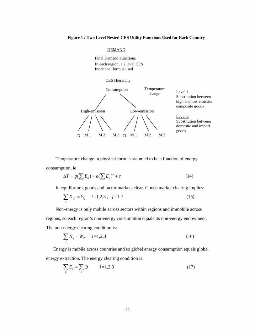
Figure 1 shows the structure of two level nested CES utility functions used.

For each good j produced in country i’, we can define the seller’s price (net of

tariff) as ijp ′ , and allow each country i to impose tariffs at rate ijit ′ ( country i ’s tariff

on good j imported from country i′ ) on each imported good. Tariffs are set to zero

for exports. Internal (gross of tariff ) prices for good j produced in country i’ are thus

'[1 ]iji jiijiP t P′ ′= + (13)

- 10 -

Temperature change in physical form is assumed to be a function of energy

consumption, ie

∑∑ +==Δ cEaEgT bijij )()( (14)

In equilibrium, goods and factor markets clear. Goods market clearing implies:

jii

iij YX ′′ =∑ i =1,2,3 , j =1,2 (15)

Non-energy is only mobile across sectors within regions and immobile across

regions, so each region’s non-energy consumption equals its non-energy endowment.

The non-energy clearing condition is:

iNj

ij WN =∑ i =1,2,3 (16)

Energy is mobile across countries and so global energy consumption equals global

energy extraction. The energy clearing condition is:

∑∑ =i

iij

ij QE i =1,2,3 (17)

DEMAND

Final Demand Functions In each region, a 2 level CES functional form is used

Level 1 Substitution between high and low emission composite goods

Level 2 Substitution between domestic and import goods

Low-emission High-emission

CES Hierarchy

Consumption Temperature change

M 2 M 3 D M 2 M 3 D

Figure 1 : Two Level Nested CES Utility Functions Used for Each Country

M 1 M 1

- 11 -

3. Data and Parameterization

We build a model compatible benchmark general equilibrium data set which we

use in calibration. Our base case assumes a single 30 year period, forward projecting a

business as usual scenario for trade, production, and consumption data (as well as

energy use) for a 2 good (energy / non energy intensive), 2 factor (energy inputs,

other inputs) structure for 4 regions (China, US , EU, ROW). We forward project

2006 data using 2004-2006 average growth rates, for the period 2006-2036.

In Table 1-1 GDP data is from the World Bank’s WDI database. The high-

emission sector reflects manufacturing industry. The low-emission sector includes

service and agricultural sectors. For Table 1-2, trade data is taken from the

UNCOMTRADE database, F.o.b. export values as reported by exporting countries

are used. Since data on EU’s exports to China and US in 2006 were not available at

the time of model execution, we use the import data of China and the US from the EU

instead. Since China’s growth rates is high relative to other regions ,to keep trade

balance in the data, we use China’s growth rate for China’s imports and exports ,

while for other data , we use the import country’s growth rate in our projections, tariff

data is from the WTO Statistical Database.

In Table 1-3 , energy data for 2005 is calculated from IEA energy statistics. The

unit of account of the IEA statistics data is thousand of tonnes of oil equivalent, which

we adjust to billion US dollars, (1 toe=7.33 barrel of oil equivalent, oil price

(average)=$ 50.64/per barrel) . In 2005, the energy balances for world were crude oil

imports of 4476208 Ktoe, while exports were 4484919 Ktoe, comparable with world

crude oil trade balance. The extraction cost is calculated using the IEA trade balance

table.

In the data presented in Table 1-4 , adjustments are made to consumption by

calculating GDP minus exports. There are also some small differences in goods

classifications between the underlying consumption, production and tariff rate data.

Table 1-5 gives energy consumption data from IEA statistics.

- 12 -

Table 1 Data Sources in Model Calibration

Table 1-1 2006-2036 GDP by Sector by Region (Billion $)

China EU-27 US ROW

High Low High Low High Low High Low

GDP by sector 250634.94 270111.98 171324.82 475585.94 156507.52 528727.91 331566.87 785626.32

GDP 520746.92 646910.76 685235.43 1117193.19

Source: World Bank’s WDI database

Table 1-2 2006-2036 Bilateral Trade Data (Billion $)

Exports by

(Billion $)

Imports by

China EU-27 US ROW World

China

High 0.00 31162.09 27276.87 77626.04 136065.00

Low 0.00 16736.03 12652.93 24385.00 53773.96

Total 0.00 47898.12 39929.80 102011.04 189838.96

EU-27

High 12539.29 0.00 13998.92 48345.62 74883.83

Low 2995.71 0.00 3426.20 15622.03 22043.94

Total 15535.00 0.00 17425.12 63967.65 96927.77

US

High 6922.08 7094.06 0.00 35001.03 49017.17

Low 3896.98 2651.82 0.00 11664.97 18213.77

Total 10819.06 9745.88 0.00 46666.00 67230.94

ROW

High 101830.79 41001.21 54236.77 0.00 197068.77

Low 26883.06 13880.83 17620.85 0.00 58384.74

Total 128713.85 54882.04 71857.62 0.00 255453.51

World

High 121292.16 79257.36 95512.56 160972.69 457034.77

Low 33775.75 33268.68 33699.98 51672.00 152416.41

Total 155067.91 112526.04 129212.54 212644.69 609451.18

Source: UNCOMTRADE database

Table 1-3 2006-2036 Energy Balance Data (Billion $)

Extrac- tion Import Export Net

Import Extraction cost Consumption

High emission sector input

Low Emission sector input

China 105558.07 13355.00 -6073.65 7281.34 -31929.23 80910.18 42907.78 38002.40

Eu27 6365.47 24024.08 -7869.24 16154.84 -1009.94 21510.37 11309.85 10200.52

US 21873.33 16281.39 -2082.20 14199.19 -5193.87 30878.64 18087.44 12791.21

ROW 137722.08 45302.26 -82937.63 -37635.37 -11553.34 88533.37 46889.71 41643.66

World 271518.94 98962.72 -98962.72 0.00 -49686.38 221832.57 119194.77 102637.79

Source: IEA energy statistics

- 13 -

Table 1-4 : Consumption of Domestic Goods (2006-2036) (Billion $) Consumption of domestic goods

High energy intensity goods

Low energy intensity goods

China 114569.94 216338.02

EU-27 96440.99 453542.00

US 107490.35 510514.14

ROW 134498.10 727241.58

Table 1-5 Energy Consumption (Billion US $)

Year China EU-27 US ROW World

2006 412.96 483.69 593.20 1446.90 2936.75

2036 80910.18 21510.37 30878.64 88533.37 221832.56

2056 612633.64 47336.00 76757.82 250518.18 987245.64

Source: International Energy Agency: Key World Energy Statistics, 2008.

As for elasticities, in the central case , model analyses elasticity parameters are

used as follows: for all countries the production elasticity is 0.5, the extraction /

energy supply elasticity is 0.5, the consumption elasticity, that is the substitution

elasticity between high and low emission goods in consumption is equal to 0.5, and

the trade elasticity ,that is the substitution elasticity between domestic and imported

goods is equal to 2. The substitution elasticities between domestic and imported

commodities follows the “rule of two”, as discussed in Hertel al. (2009). This rule

was first proposed by Jomini et al.(1991) and later tested by Liu, Arndt,and

Hertel(2002) in a back-casting exercise with a simplified version of the GTAP model.

The model Global 2100 uses a capital and labour nest against energy with a

substitution elasticity of 0.4 (see Manne and Richels, 1992), Kemfert(1998) studied

the case of Germany, and the substitution elasticities in all sectors between composite

of capital and labor , trading off against energy was 0.458. We thus use the setting of

0.5 as the substitution elasticity between energy and non-energy inputs.

- 14 -

Using the data for 2006,2036, and 2056 in table 1-5, and assuming the

temperature change at these three points to be 0℃,2℃, and 5℃ respectively, we can

solve for the values of parameters a,b,and c in equation (14) as

ca += b2936.75)-2936.75(0

ca += b221832.56)(2

ca += b) 987245.64(5

Solving these equations for the parameters a,b,and c yields values of 0.0010,

0.6137 and 0. Substituting these values in the temperature equation yields

∑∑ ==Δ 0.6137)(0.001)( ijij EEgT (18)

Assuming a temperature change TΔ of 5℃ between 2006 and 2056 (consistent

with Stern(2002)), Table 2 reports the calibrated preference parameters in equation (9)

under alternative damage assumptions. If we assumed half temperature change, at

these three points to be 0℃,1℃, and 2.5℃ respectively, we can solve for the values

of parameters a,b,and c, 0.0005, 0.6137 and 0. If we double temperature change,

temperature change at these three points will be 0℃,4℃, and 10℃ respectively, and

the values of parameters a,b,and c are 0.0021 , 0.6137, and 0 .

The specification C can be thought of the global temperature change at which all

economic activity ceases (say 20℃). In this case, as TΔ approaches C utility goes to

zero. In this form , as TΔ goes to zero there is no welfare impact of temperature

change. As discussed in Cai et al.(2009), the share parameter β reflects the assumed

severity of damage from temperature change, which we later (in Table 7) calibrate to

various damage estimates from business as usual global temperature change scenarios

reported by Stern(2006) and Mendelson(2007).

Table 2 also reports remaining parameter values in production, preferences and

extraction cost functions generated by calibration. These are independent of the

assumed utility damage due to temperature change.

- 15 -

Table 2 Calibrated Parameters under Alternative Damage Assumptions A． Assumed Changes in Preference Parameters

Assumed Utility Loss Utility Relative to No damage β

1% 0.99 0.0349

1.5% 0.985 0.0525

3% 0.97 0.1059

5% 0.95 0.1783

6% 0.94 0.2151

10% 0.90 0.3662

15% 0.85 0.5649

20% 0.80 0.7757

B． Parameters in CES production functions China EU US ROW

high

emission goods

low emission

goods

high emission

goods

low emission

goods

high emission

goods

low emission

goods

high emission

goods

low emission

goods

technology coefficient

1.39621179 1.31890362 1.14065722 1.04381582 1.25695383 1.04955396 1.32072255 1.11159828

shares on energy

0.20228798 0.16157483 0.07050406 0.02191317 0.12956913 0.02478459 0.16252202 0.05588649

shares on non-energy 0.97932608 0.98686046 0.99751149 0.99975988 0.99157039 0.99969281 0.98670492 0.99843713

C. Parameters in Nested CES Utility functions China EU US ROW

Shares of consumption of high emission domestic and import goods

China-H 0.14174185 0.05360871 0.03921093 0.07263893

EU-H 0.01843119 0.15398406 0.02012367 0.04523964

US-H 0.01017459 0.01220404 0.14508505 0.03275238

ROW-H 0.14967854 0.07053513 0.0779662 0.11344204

Shares of consumption of low emission domestic and import goods

China-L 0.34606345 0.02140224 0.01314736 0.01844225

EU-L 0.00642599 0.4385596 0.00356008 0.01181486

US-L 0.00835927 0.00339118 0.47659601 0.00882215

ROW-L 0.05766585 0.01775098 0.01830941 0.43768184

China EU US ROW

Shares of high and low emission composite goods

high

emission goods

low emission

goods

high emission

goods

low emission

goods

high emission

goods

low emission

goods

high emission

goods

low emission

goods

0.64095368 0.76757956 0.27094705 0.96259425 0.26848974 0.96328254 0.27433175 0.96163511

D. Parameters in Extraction functions Constant

Parameter -38442.80 -3233.71 -9388.35 -80261.40

Coefficient parameter 0.00205193 0.00835591 0.00450766 0.00179642

- 16 -

4 . Model Experiments and Results for Carbon Motivated Regional

Trade Agreements We have used our calibrated model to simulate the impacts of carbon motivated

regional trade agreements on emissions and welfare. Following Dong & Whalley

(2008), we analyze the first type of carbon motivated regional agreement (lower

tariffs on low carbon intensive goods) and the third types of carbon motivated

regional agreements(added penalties on third parties). Results are presented in Table 3

to Table 8.

These experiments confirmed the conjectures in our previous policy paper (see

Dong & Whalley (2008)), that while carbon motivated regional agreements can

reduce global carbon emissions, the effect on carbon emissions is small. Carbon

motivated regional agreements may increase world welfare, but the effects on

participating countries may be negative or positive. When we consider third party

penalties, the effects of carbon motivated trade policies on carbon emissions are still

small. Even though carbon motivated regional agreements will have larger effects on

emissions when high and low emissions countries are involved compared to more

uniform emissions levels, the effects are still small.

In Tables 3,4,5, using central case model specifications, we analyze four

groupings of regional trade agreements, these are EU-US, EU-China, US-China, and

EU-US-China. In each group, there are two sub forms. One is carbon free trade

agreements, which eliminates interior tariffs on low carbon intensive goods, and keep

tariffs on high carbon intensive goods unchanged. The other is carbon motivated

customs unions, besides within region tariff reductions as in carbon free trade

agreements, we assume a common 5% external tariff on low carbon motivated goods.

Totally we analyze eight kinds of carbon motivated regional trade agreements in our

central case analyses.

Table 3 reports the impacts of carbon motivated trade arrangements on welfare

and emissions. Most carbon motivated trade arrangements will reduce global

emissions, but the effect is small. In Table 3-1, the global emissions are reduced in

seven cases; the exception being in the US-China carbon CU case. The biggest

reduction is from a EU-US-China carbon FTA, -0.0221% (very small change), and

smallest reduction is from a EU-US carbon FTA, -0.0008%, Since China has much

- 17 -

higher emissions intensity than the EU or the US, the carbon FTAs that involve China

will have larger effects.

We can also compare carbon FTAs and carbon CUs. In case 1 and case 4,

EU-US, EU-US-China, since China and ROW are respectively outside the agreement

and both of these two regions have a higher emission intensity than the insiders

(measured in average emissions intensity across sectors), carbon CUs has more

impact than carbon FTAs in these two scenarios. In cases 2 and 3, EU-China,

US-China, the outside countries have lower emissions levels than insiders (average

level). In this case carbon FTAs have more impacts on emissions than a carbon CU. A

carbon CU has a larger role than a carbon FTA in reducing carbon emissions when

the outsider has higher emission intensity than insiders.

Table 3-1 also reports separate effects on country’s emissions. The EU increases

emissions in most cases, since EU’s carbon intensity is low, and increased trade

increases production in other member countries who have a relative higher carbon

intensity. For China, participating in the carbon free trade areas will decrease China’s

carbon emissions, such that EU-China carbon FTA, US-China carbon FTA ,

EU-US-China FTA will decrease China’s emissions 0.0227%, 0.0002%, 0.0202%.

For US, in most cases, participating in carbon FTAs and CUs will reduce it’s carbon

emissions.

In Table 3-2, for welfare analysis, we use Hicksian CV and EV measures

capturing the effects of temperature change.

1 0

0 0( ) ( )

i i ii

i i

i i

U U UCV C T C TC C

β β

Δ −= =

−Δ −Δ (19)

1 0

1 1( ) ( )

i i ii

i i

i i

U U UEV C T C TC C

β β

Δ −= =

−Δ −Δ (20)

In Table 3-2, since the temperature change is small, 0 1T TΔ ≈ Δ , and CV and EV

measures from equations (19) and (20) are similar. We only focus on the CV measure.

For the global economy, in most cases (except a US-China carbon FTA), carbon

motivated regional trade agreements are welfare improving. And comparing carbon

FTA and CU, in case 1, since the outsider has higher carbon emissions, the total

welfare increase is small, for a EU-US FTA, when reducing the tariff on outsider’s

low carbon goods to a 5% CET , A EU-US CU however, seems to improve global

- 18 -

welfare more. In cases 2,3 and 4, the high emission country China is involved in the

carbon arrangement, so a carbon CU is more powerful than carbon FTAs in increasing

global welfare. For insiders, in EU-US FTA/CU, EU-China FTA/CU , EU-US-China

FTA/EU, the EU will benefit most from these arrangements, in US-China CU, China

will benefit most. For outsiders, in all cases, outsiders increase welfare in carbon

FTAs, but lose in a carbon CU.

Table 3-1 Impacts of Carbon Motivated Trade Agreements on Emissions(Energy Use)

(% Change Based on 2006 Data)

Carbon FTA/CU % Change in Emissions

China EU US Row Total

1 EU-US FTA 0.0029% 0.0102% -0.0266% 0.0013% -0.0008%

EU-US CU ( 5 % CET) -0.0123% 0.1761% -0.0019% -0.0711% -0.0162%

2 EU-China FTA -0.0227% 0.1342% 0.0437% -0.0715% -0.0186%

EU-China CU( 5 % CET) 0.0174% 0.1576% -0.0975% -0.0509% -0.0090%

3 US-China FTA -0.0002% 0.0063% -0.0069% -0.0067% -0.0027%

US-China CU (5 % CET) 0.0311% -0.0695% -0.0627% 0.0268% 0.0103%

4 EU-US-China FTA -0.0202% 0.1509% 0.0114% -0.0771% -0.0221%

EU-US-China CU ( 5 % CET) 0.0108% 0.1591% -0.0569% -0.0695% -0.0130%

- 19 -

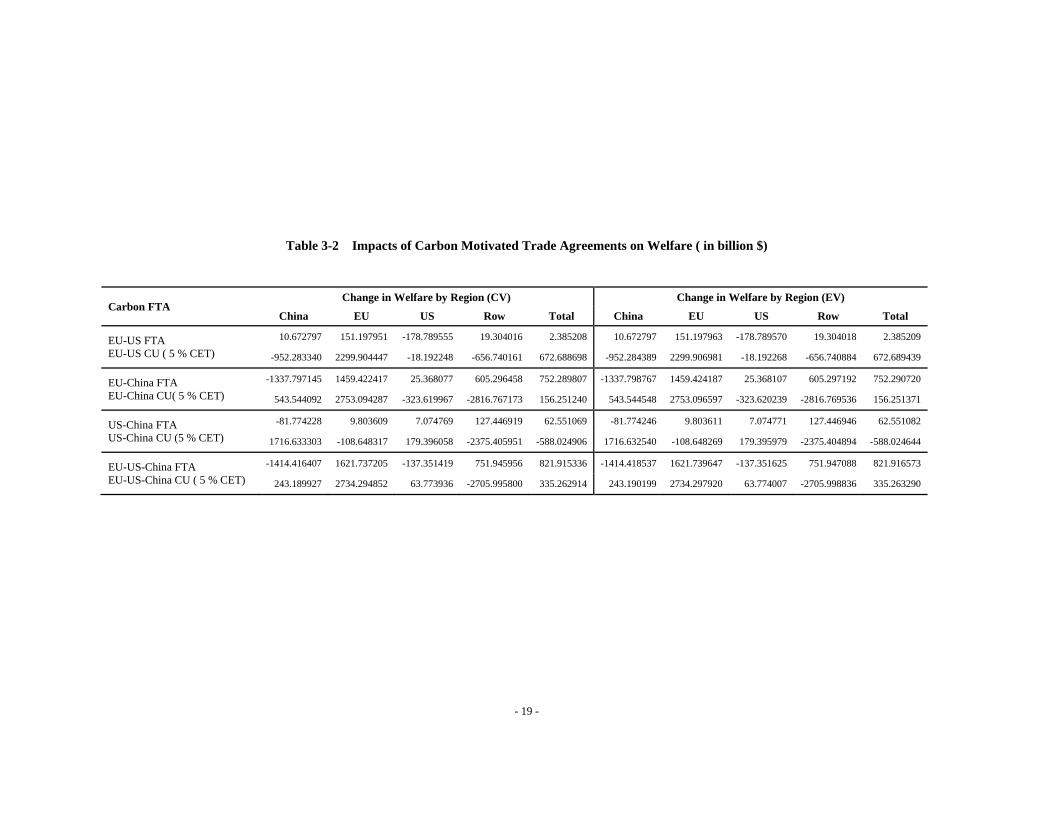
Table 3-2 Impacts of Carbon Motivated Trade Agreements on Welfare ( in billion $)

Carbon FTA Change in Welfare by Region (CV) Change in Welfare by Region (EV)

China EU US Row Total China EU US Row Total

EU-US FTA 10.672797 151.197951 -178.789555 19.304016 2.385208 10.672797 151.197963 -178.789570 19.304018 2.385209

EU-US CU ( 5 % CET) -952.283340 2299.904447 -18.192248 -656.740161 672.688698 -952.284389 2299.906981 -18.192268 -656.740884 672.689439

EU-China FTA -1337.797145 1459.422417 25.368077 605.296458 752.289807 -1337.798767 1459.424187 25.368107 605.297192 752.290720

EU-China CU( 5 % CET) 543.544092 2753.094287 -323.619967 -2816.767173 156.251240 543.544548 2753.096597 -323.620239 -2816.769536 156.251371

US-China FTA -81.774228 9.803609 7.074769 127.446919 62.551069 -81.774246 9.803611 7.074771 127.446946 62.551082

US-China CU (5 % CET) 1716.633303 -108.648317 179.396058 -2375.405951 -588.024906 1716.632540 -108.648269 179.395979 -2375.404894 -588.024644

EU-US-China FTA -1414.416407 1621.737205 -137.351419 751.945956 821.915336 -1414.418537 1621.739647 -137.351625 751.947088 821.916573

EU-US-China CU ( 5 % CET) 243.189927 2734.294852 63.773936 -2705.995800 335.262914 243.190199 2734.297920 63.774007 -2705.998836 335.263290

- 20 -

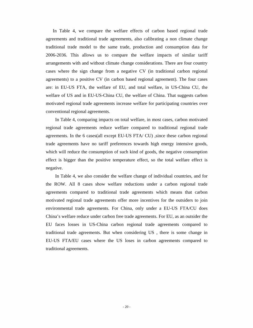
In Table 4, we compare the welfare effects of carbon based regional trade

agreements and traditional trade agreements, also calibrating a non climate change

traditional trade model to the same trade, production and consumption data for

2006-2036. This allows us to compare the welfare impacts of similar tariff

arrangements with and without climate change considerations. There are four country

cases where the sign change from a negative CV (in traditional carbon regional

agreements) to a positive CV (in carbon based regional agreement). The four cases

are: in EU-US FTA, the welfare of EU, and total welfare, in US-China CU, the

welfare of US and in EU-US-China CU, the welfare of China. That suggests carbon

motivated regional trade agreements increase welfare for participating countries over

conventional regional agreements.

In Table 4, comparing impacts on total welfare, in most cases, carbon motivated

regional trade agreements reduce welfare compared to traditional regional trade

agreements. In the 6 cases(all except EU-US FTA/ CU) ,since these carbon regional

trade agreements have no tariff preferences towards high energy intensive goods,

which will reduce the consumption of such kind of goods, the negative consumption

effect is bigger than the positive temperature effect, so the total welfare effect is

negative.

In Table 4, we also consider the welfare change of individual countries, and for

the ROW. All 8 cases show welfare reductions under a carbon regional trade

agreements compared to traditional trade agreements which means that carbon

motivated regional trade agreements offer more incentives for the outsiders to join

environmental trade agreements. For China, only under a EU-US FTA/CU does

China’s welfare reduce under carbon free trade agreements. For EU, as an outsider the

EU faces losses in US-China carbon regional trade agreements compared to

traditional trade agreements. But when considering US , there is some change in

EU-US FTA/EU cases where the US loses in carbon agreements compared to

traditional agreements.

- 21 -

Table 4 Comparing Conventional CU / FTA Analysis and Carbon Based Regional Trade Agreement Analysis(billion $)

Carbon FTA/CU

Carbon Based Regional Agreement Analysis : Change in Welfare by Region (CV)

Conventional Regional Agreements Analysis : Change in Welfare by Region (EV)


EU-US FTA 10.672797 151.197951 -178.789555 19.304016 2.385208 63.895291 -24.256359 -171.007329 106.121569 -25.246827 EU-US CU ( 5 % CET) -952.283340 2299.904447 -18.192248 -656.740161 672.688698 -897.757238 2122.934557 -11.926031 -568.811030 644.440258

EU-China FTA -1337.797145 1459.422417 25.368077 605.296458 752.289807 -1583.533067 1216.959514 60.438650 1164.303098 858.168195 EU-China CU( 5 % CET) 543.544092 2753.094287 -323.619967 -2816.767173 156.251240 294.330273 2497.693855 -287.134231 -2240.576825 264.313073

US-China FTA -81.774228 9.803609 7.074769 127.446919 62.551069 -349.715881 51.949010 -51.645805 531.011861 181.599184 US-China CU (5 % CET) 1716.633303 -108.648317 179.396058 -2375.405951 -588.024906 1445.527652 -65.896454 113.499567 -1961.025906 -467.895142

EU-US-China FTA -1414.416407 1621.737205 -137.351419 751.945956 821.915336 -1879.439131 1252.433868 -140.989771 1794.158006 1026.162972 EU-US-China CU ( 5 % CET) 243.189927 2734.294852 63.773936 -2705.995800 335.262914 -226.735896 2352.761394 52.656415 -1636.997994 541.683920

- 22 -

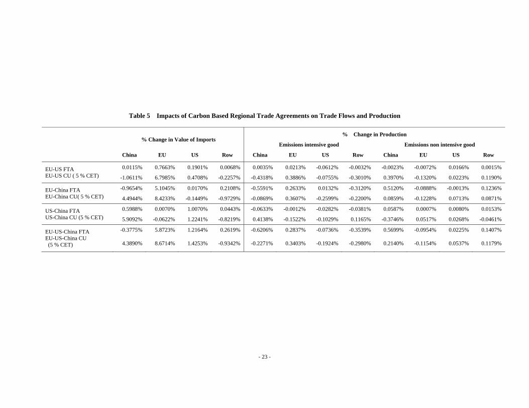
In Table 5 , we analyze the impacts of carbon based regional trade agreements on

trade flows and production. In nearly all eight cases, carbon FTA/CU will increase

insider’s imports, except in the case of EU-China carbon FTA for China, and the

EU-US-China FTA for China. For outsiders the results are that carbon FTAs will

increase outsider’s imports, but a carbon CU (5% CET) will reduce outsider’s

imports.

Table 5 also reports the impacts on production in nearly all cases. China, US, Row

increase low energy intensive goods, production, and reduce high energy intensive

goods production, except in an EU-US FTA(China production), a US-China CU

(China ,ROW Production), a EU-China FTA(US production). As for the EU, except

for US-China a FTA/CU increases low energy intensive goods production, and

reduces high energy intensive goods production. In all other cases ,the EU reduces

low energy intensive goods production and increases high energy intensive goods

production. That means that high emission countries will tend to produce more low

energy intensive goods, and less high energy intensive goods, no matter whether they

are outsiders or insiders. For a low emission country (EU), when it is an outsider, it

will tend to produce more low energy intensive goods, and less high energy intensive

goods, and when it is an insider, vice versa. That means if carbon regional trade

agreements are signed between high emission countries, it will be more forceful in

reducing carbon emissions.

- 23 -

Table 5 Impacts of Carbon Based Regional Trade Agreements on Trade Flows and Production

% Change in Value of Imports

% Change in Production

Emissions intensive good Emissions non intensive good

China EU US Row China EU US Row China EU US Row

EU-US FTA 0.0115% 0.7663% 0.1901% 0.0068% 0.0035% 0.0213% -0.0612% -0.0032% -0.0023% -0.0072% 0.0166% 0.0015% EU-US CU ( 5 % CET) -1.0611% 6.7985% 0.4708% -0.2257% -0.4318% 0.3886% -0.0755% -0.3010% 0.3970% -0.1320% 0.0223% 0.1190%

EU-China FTA -0.9654% 5.1045% 0.0170% 0.2108% -0.5591% 0.2633% 0.0132% -0.3120% 0.5120% -0.0888% -0.0013% 0.1236% EU-China CU( 5 % CET) 4.4944% 8.4233% -0.1449% -0.9729% -0.0869% 0.3607% -0.2599% -0.2200% 0.0859% -0.1228% 0.0713% 0.0871%

US-China FTA 0.5988% 0.0070% 1.0070% 0.0443% -0.0633% -0.0012% -0.0282% -0.0381% 0.0587% 0.0007% 0.0080% 0.0153% US-China CU (5 % CET) 5.9092% -0.0622% 1.2241% -0.8219% 0.4138% -0.1522% -0.1029% 0.1165% -0.3746% 0.0517% 0.0268% -0.0461%

EU-US-China FTA -0.3775% 5.8723% 1.2164% 0.2619% -0.6206% 0.2837% -0.0736% -0.3539% 0.5699% -0.0954% 0.0225% 0.1407% EU-US-China CU (5 % CET) 4.3890% 8.6714% 1.4253% -0.9342% -0.2271% 0.3403% -0.1924% -0.2980% 0.2140% -0.1154% 0.0537% 0.1179%

- 24 -

In Table 6-1, we report sensitivity results for elasticities and other key model

parameters for carbon based regional trade agreements analysis. If we choose the case

of a EU-US-China carbon FTA, decreasing trade elasticities increases the global

emissions impact of the agreement. The outsider increases emissions, and for the

insider, China emissions increases, while EU and US reduce emissions. Decreasing

production elasticities, all insiders will reduce emissions, but for outsiders, the result

is not clear. Reducing extraction elasticities, all regions increase emissions. With a

combined reduction of trade elasticities, production elasticities and extractions

elasticities together, total emissions increase, and outsiders still increase emissions,

and for the insiders, EU and US emissions fall while the China increases emissions.

In Table 6-2, when considering welfare inputs, lower trade elasticities will

increase all regions welfare impacts, and a fall in production elasticities increases the

welfare of EU,US and ROW and decreases the welfare of the China and total welfare.

Also a fall in extraction elasticities will increase the welfare of EU, US, Row, and

decrease the welfare of the China and total welfare. With a combined reduction of

trade elasticities, production elasticities and extractions elasticities together, all

regions welfare impacts of trade agreements will increase.

Table 6-1 Sensitivity of Carbon Based Regional Trade Agreements Analysis to Elasticities and Other Key Model Parameters (% change based on 2005 data)

EU-US-China FTA % Change in emissions

China EU US Row Total

1. Base Case ( Table 3-1)

2 1.5 trade elasticities in all regions -0.0146% 0.1146% 0.0084% -0.0405% -0.0105%

3 Half trade elasticities in all regions 0.0133% -0.0993% -0.0105% 0.0357% 0.0092%

4 Double production substitution elasticities in all regions

0.0112% 0.0958% 0.1412% -0.0721% 0.0065%

5 Half production substitution elasticities in all regions

-0.0114% -0.0126% -0.0108% -0.0113% -0.0114%

6 Double the extractions elasticities in all regions -0.0081% -0.0078% -0.0080% -0.0081% -0.0081%

7 Half the extractions elasticities in all regions 0.0001% 0.0001% 0.0001% 0.0001% 0.0001%

8 2,4, and 6 together -0.0115% 0.1222% 0.0142% -0.0394% -0.0074%

9 3,5,and 7 together 0.0061% -0.1068% -0.0172% 0.0286% 0.0020%

- 25 -

Table 6-2 Sensitivity of Carbon Based Regional Trade Agreements Analysis to Elasticities and Other Key Model Parameters (billion $)

EU-US-China FTA CV EV China EU US Row Total China EU US Row Total

1 Base Case ( Table 3-2)

2 1.5 trade elasticities in all regions -11884.33 -33674.22 -39881.21 -52711.38 -138151.13 -11884.33 -33674.24 -39881.23 -52711.41 -138151.22

3 Half trade elasticities in all regions 28332.00 81356.55 90683.11 130990.17 331361.84 28331.99 81356.51 90683.07 130990.10 331361.66

4 Double production substitution elasticities in all regions

-15.79 200.32 -1053.23 -327.36 -1196.06 -15.79 200.32 -1053.23 -327.36 -1196.06

5 Half production substitution elasticities in all regions

-8.29 4.24 1.41 0.51 -2.12 -8.29 4.24 1.41 0.51 -2.12

6 Double the extractions elasticities in all regions

0.39 -1.72 -1.31 -2.12 -4.76 0.39 -1.72 -1.31 -2.12 -4.76

7 Half the extractions elasticities in all regions

0.00 0.00 0.00 0.00 0.00 0.00 0.00 0.00 0.00 0.00

8 2,4, and 6 together -11876.01 -33683.83 -39885.16 -52703.61 -138148.61 -11876.02 -33683.84 -39885.17 -52703.63 -138148.66

9 3,5,and 7 together 28327.44 81358.23 90683.47 130989.70 331358.85 28327.44 81358.23 90683.47 130989.69 331358.83

- 26 -

Table 7 Sensitivity of Results to Key Parameters in the Environmental Component of Modeling Structure (billion $)

EU-US-China FTA (CV) EU- China FTA( CV)


1 Base Case ( Table 3-2) 473.88 997.74 1162.91 1549.24 4183.77 476.42 1003.10 1169.15 1557.56 4206.24

2 Halve damage estimated to calibrate preferences towards temperature change

-977.00 -2057.01 -2397.68 -3193.98 -8625.67 -966.35 -2034.60 -2371.56 -3159.18 -8531.70

3 Double damage estimated to calibrate preferences towards temperature change

481.65 1014.14 1181.90 1574.53 4252.22 484.28 1019.68 1188.36 1583.13 4275.44

4 Halve temperature change for BAU scenario -1166.54 -104853.31 -2862.82 -3813.58 -112696.25 -1151.40 -103492.22 -2825.66 -3764.08 -111233.35

5 Double temperature change for BAU scenario 473.88 997.74 1162.91 1549.24 4183.77 476.42 1003.10 1169.15 1557.56 4206.24

- 27 -

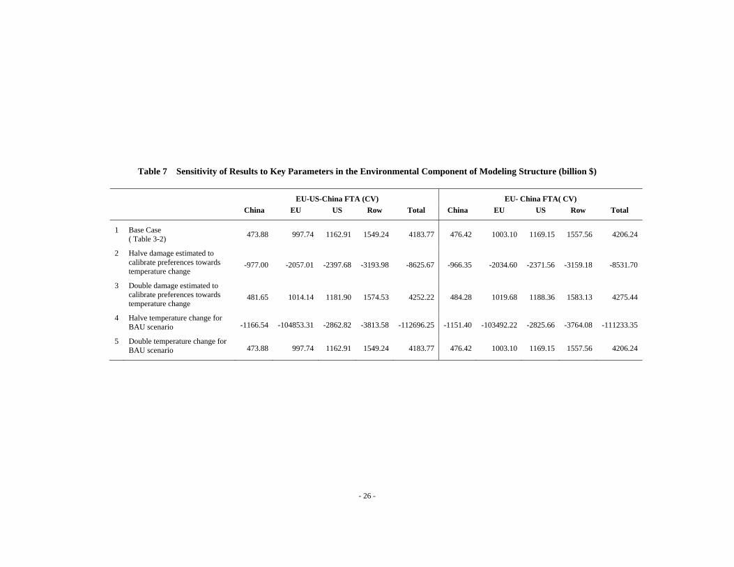
Table 7 reports sensitivity analysis of key parameters in the environmental

component of the modeling structure. We choose two cases, EU-US-China FTA and

EU-China FTA, both cases show that if we increase damage cost estimates, the

welfare impacts will increase. And also if we increase temperature change,the welfare

impacts of agreements will increase with increasing temperature change.

In Table 8 ,we analyze the impacts of carbon based regional trade agreements on

emissions and welfare with trade penalties on third parties. Results show that

increasing penalties on outsiders effectively decreases the emissions of outsiders, but

increase the emission of insiders, and also increase the world total emissions. The

EU-US FTA involves zero tariff on low emission goods, increasing domestic

production (and consumption) of high emission goods. Imports from China of high

emission goods fall, and emissions rise in the EU and the US. Interestingly, there are

peaks for the implied emissions reduction as a function of external penalty rates,

suggesting an optimal external tariff in terms of maximizing emissions reduction.

Table 8 Impacts on Emissions of Carbon Based Regional Trade Agreements with Penalties (billion $)

EU-US FTA

% Change in Emissions China EU US Row Total

1 FTA without penalty 0.0029% 0.0102% -0.0266% 0.0013% -0.0008%

2 15% external rate on high emission goods -0.1525% 1.4337% 2.0618% -1.0050% -0.0352%






8 15% external rate on all goods -0.1325% 1.4400% 1.8748% -0.9476% -0.0299%




12 150% external rate on all goods -1.0810% 8.3110% 12.1237% -4.9175% 0.0243%

13 200% external rate on all goods -1.2836% 9.4075% 13.8343% -5.4330% 0.0572%

- 28 -

5. Concluding Remarks

We build on an earlier policy piece by Dong & Whalley(2008) and develop a

multi-region general equilibrium model calibrated to a single period data set reflecting

a business as usual scenario between 2006 and 2036. We use this to evaluate the

impacts of both carbon motivated free trade agreements and customs unions on trade,

emissions and welfare. Our results confirm the widely held view that as a mechanism

for reducing carbon emissions trade policy would seem to only offer quantitatively

small and indirect effects, since it is economic growth more so than trade and its

composition that seemingly fuels growing emissions.

Results from model analysis show that carbon motivated trade arrangements may

reduce global carbon emissions. And as conjectured by Dong & Whalley(2008), the

effect of such agreements on emissions are relatively small comparing carbon FTAs

and carbon CU, carbon CUs seem more powerful than carbon FTAs in terms of

emissions impacts when outsiders have higher emission intensities than insiders.

For welfare analysis , most carbon RTAs are welfare improving. When including

high emission countries in the agreements, carbon based CUs are more effective than

carbon FTAs. Comparing carbon RTAs to traditional RTAs, since carbon RTAs do

not eliminate tariffs on high emission goods, the negative consumption effect is

bigger than the positive temperature effects, so the total welfare effect is negative.

Carbon RTAs also give a much bigger incentive than traditional RTAs for the

outsider to join agreements. In most cases, carbon based RTAs will increase insider’s

imports, For outsiders , the impacts on imports are unclear: carbon based RTAs will

increase the production of low energy intensive goods, and reduce the production of

high energy intensive goods; Finally even with trade penalties on third parties there

are still not large effects in terms of carbon emissions reductions

As the global debate on a new Post 2012 climate change regime moves forward

to the 2009 Copenhagen UNFCCC negotiation, trade and climate issues will likely

link prominently. These results seemingly support the general argument that as a way

of addressing climate change, trade policy has only small impacts.

- 29 -

References Bhattacharyya, S.C.(1996) “Applied General Equilibrium Models for Energy Studies:

A Survey”, Energy Economics ,Vol18 (1996),pp.145-164. Cai,Y,Z, R.Riezman and J. Whalley(2009) “International Trade and the Negotiability

of Global Climate Change Agreements” , NBER Working Paper No.14711, Issued in Feb 2009.

Chatham House (2007) “Changing Climates: Interdependencies on Energy and

Climate Security for China and Europe”, Antony Froggatt, Bernice Lee, Chatham House Report.

Cooke,R.(2007) “The elasticity of oil production and consumption”, Energy Bulletin,

Archived Mar 22 2007. Dong,Y. & J. Whalley (2008) “Carbon, Trade Policy, and Carbon Free Trade Areas”,

NBER Working Paper No.14431, Issued in October 2008. Hertel, T., R. McDougall, B.Narayanan and A.H. Aguiar(2009)“GTAP 7 Data Base

Documentation - Chapter 14: Behavioral Parameters”, access at https://www.gtap.agecon.purdue.edu/resources/download/4184.pdf

Jomini, P., J.F. Zeitsch, R. McDougall, A. Welsh, S. Brown, J.Hambley and J.

Kelly(1991) “SALTER: A General Equilibrium Model of the World Economy”, Vol. 1. Model Structure, Data Base, and Parameters. Canberra, Australia: Industry Commission.

Kemfert,C.(1998)“Estimated Substitution Elasticities of a Nested CES Production

Function Approach for Germany. Energy Economics 20 3, pp. 249–264. Kemp M. and H. Wan (1976)“An Elementary Proposition Concerning the Formation of Customs Unions”. Journal of International Economics 6,pp.95-97.

Lipsey,R.G. & Kelvin Lancaster(1956)“The General Theory of Second Best”, The

Review of Economic Studies, Vol. 24, No. 1. (1956 - 1957), pp. 11-32. Lipsey, R. G. (1957) “The Theory of Customs Unions: Trade Diversion and Welfare”,

Economica 24, pp40-46. Lipsey, R. G. (1970), The Theory of Customs Unions: A General Equilibrium

Analysis. London: Weidenfeld and Nicholson. Liu, J., Y. Surry, B. Dimaranan and T. Hertel(1998) “CDE Calibration,” Chapter 21

in Robert McDougall, Aziz Elbehri, and Truong P. Truong. Global Trade, Assistance and Protection: The GTAP 4 Data Base, Center for Global Trade Analysis, Purdue University, West Lafayette, Indiana.

- 30 -

Lockwood B. & J. Whalley (2008) “Carbon Motivated Border Tax Adjustments: Old Wine in Green Bottles?” NBER Working Paper No. 14025 , Issued in May 2008 .

Manne, A. S. and R. G. Richels(1999) “The Kyoto Protocol: A Cost-Effective

Strategy for Meeting Environmental Objectives?” in The Costs of the Kyoto Protocol: A Multi-Model Evaluation, John Weyant (ed.), Special Issue of The Energy Journal.

Meade, J.E.(1955) The Theory of Customs Unions. North Holland, Amsterdam. Mendelsohn, Robert, O.(2006) A Critique of the Stern Report, Regulation.(Winter

2006-2007), pp.42-46. OECD(1993) “GREEN: The Technical Reference Manual”, Economics Department,

OECD Paris, October, 1993. Riezman, R. (1979), “A 3x3 Model of Customs Unions”. Journal of International Economics 9,pp.341-354. Stern,N. (2006) Stern Review on the Economics of Climate Change. (Cambridge Univ

Press, Cambridge, UK). Viner J. (1950) The Customs Union Issue, New York: Carnegie Endowment for

International Peace. Walsh, S. & J. Whalley (2008) “The Global Negotiating Framework for Climate

Change Mitigation”, paper prepared at CESifo conference in Venice July 2008 on European Global Environmental Negotiations.

Wing, I. S.(2004) “Computable General Equilibrium Models and Their Use in

Economy-Wide Policy Analysis”, MIT Technical Note No. 6, September 2004.

Carbon Motivated Regional Trade Arrangements: Analytics ... filetrade agreements, by lowing tariffs...

Documents

Transcript of Carbon Motivated Regional Trade Arrangements: Analytics ... filetrade agreements, by lowing tariffs...