CARBON DIOXIDE AND CLIMATE: A SCIENTIFIC ASSESSMENTJule G. Charney, Akio Arakawa, D. James Baker, Bert Bolin, Robert E. Dickinson,

Richard M. Goody, Cecil E. Leith, Henry M. Stommel, Carl I. Wunsch

July 27, 1979

KEY POINTS

‘Incontrovertible evidence’ human activity is changing the atmosphere.

A wait-and-see policy means waiting until it is too late.

When will CO2 double? 2030—2050.

All models mutually supporting: 5 of 5 models predict warming.

Upper bound from H1: +3.5° (Over-estimation of water vapour feedback)Lower bound from M series: +2° (Under-estimation of water vapour feedback)

Best estimate of surface temperature change? +3° degrees (probable error of ±1.5°)

A historical document: Jules Charney and Jimmy Carter.

Conclusions are comforting for scientists and disturbing for policy makers.

Conclusions have generally held: +2.6°—4.1° clustering around +3°C.3

CO2 LEVELS

1850: ~290

1958: 314

1979: 334

2013: 395

2050: 580?

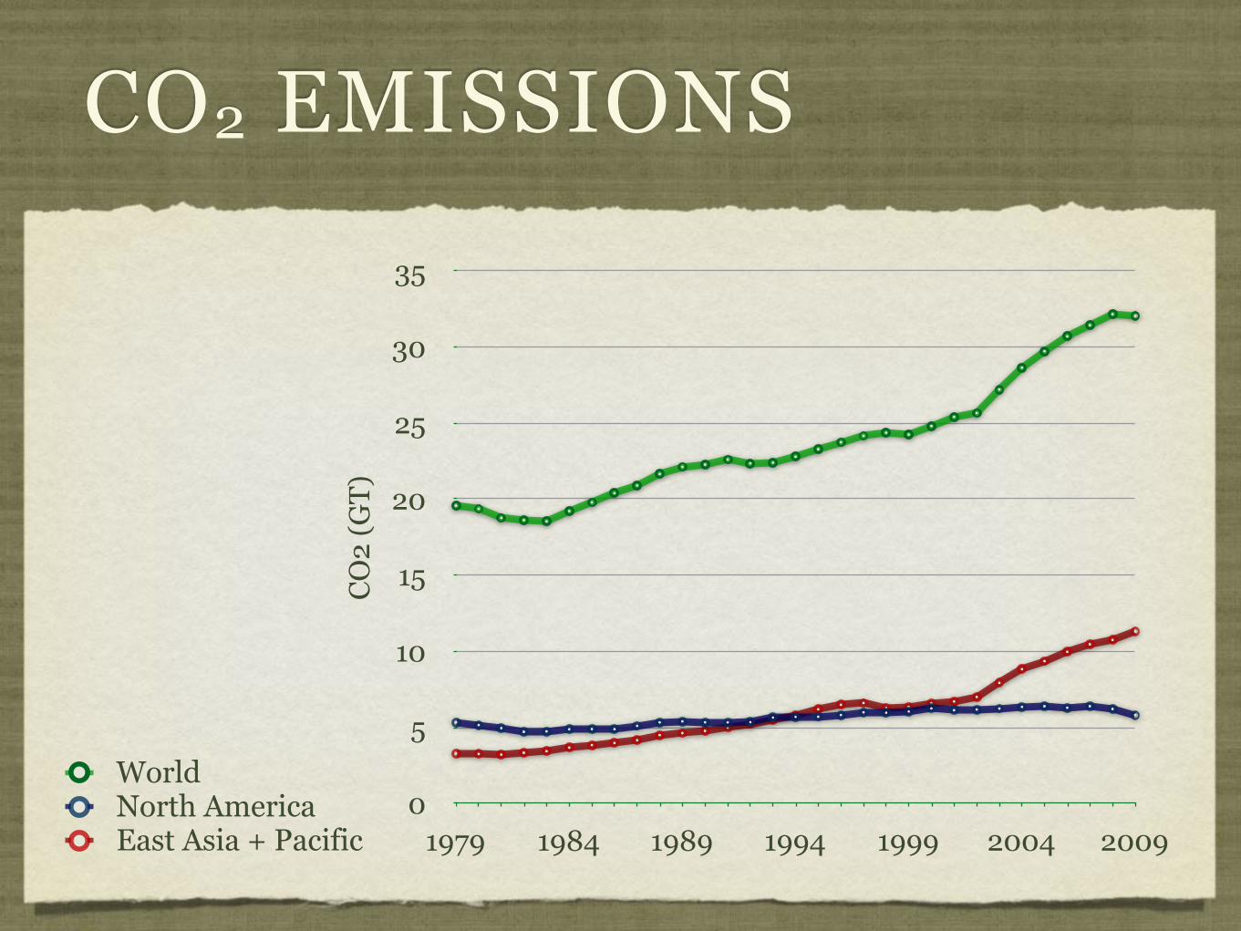
CO2 EMISSIONS

0

5

10

15

20

25

30

35

1979 1984 1989 1994 1999 2004 2009

CO2

(GT)

WorldNorth AmericaEast Asia + Pacific

ASSUMPTIONS

~50% of CO2 stays in Atmosphere, the rest is absorbed by Forests and Oceans.

Positive feedback from moisture will overwhelm all conceivable negative feedback mechanisms.

Fossil Fuel Consumption: 2% increase (1.9% actual1).

Fossil Fuel Reserves: 5000 x 109 — 10% is Oil and Gas (As of 20112: 3600 x 109 — 21.8% is Oil and Gas)

DETAILS

∆Q = Change in Heating of Troposphere, Oceans, and Land (RF). ∆Q = 4Wm-2 ±25% (2001 IPCC revised to 3.7W/m2)

W = Amount of Sunlight?

∆T = Change in Surface Temperature.∆T = ∆Q/Ø,

Ø = effect of feedback processes: Humidity, AlbedoØ = 1.7±0.8 Wm-2 K-1 or about 2.4 K

K = Amount of Heat?

Limitations:Carbon Cycle, Clouds, Heat Transport in Oceans, Simple Feedback models.

THE MODELS

Model CharacteristicsModel PredictionsModel PredictionsModel PredictionsModel PredictionsModel Predictions

Model CharacteristicsM1a M2a M3a H1b H2b

Domain 0°<λ<120°, 0°<ø<81.7°c 0°<λ<120°, 0°<ø<90°c Global Global Global

Land-ocean distribution Ocean for 60°<λ<120°, 0°<ø<66.5°

Ocean for 60°<λ<120°, 0°<ø<90° Realistic Realistic Realistic

Ocean Swamp Swamp Mixed layer Mixed layer Swamp

Seasonal change No No Yes Yes No

Cloud feedbacks No Yes No Yes Yes

Snow and ice albedo 

When T<−25°C: 0.7When T>−25°C:0.45 for snow0.35 for ice

When T<−10°C: 0.7When T>−10°C:0.45 for snow0.35 for ice

Depends on depth and underlying surface albedoFor deep snow, 0.8For thick ice, 0.7

For snow, depends on snow age, snow depth, underlying surface albedo, etc.For ice, 0.45

Same as H1 

Horizontal resolution About 500 km on a mercator projection

5° in longitude4.5° in latitude

Spectral model with the maximum zonal wave number 15

10° in longitude8° in latitude Same as H1

Vertical resolution 9 layers 9 layers 9 layers 7 layers 7 layers

a Models developed by S. Manabe and colleagues at the NOAA Geophysical Fluid Dynamics Laboratory, Princeton, N.J.b Models developed by J. Hansen and colleagues at the NASA Goddard Institute for Space Studies, New York, N.Y.c Cyclic continuity assumed at boundaries.

a Models developed by S. Manabe and colleagues at the NOAA Geophysical Fluid Dynamics Laboratory, Princeton, N.J.b Models developed by J. Hansen and colleagues at the NASA Goddard Institute for Space Studies, New York, N.Y.c Cyclic continuity assumed at boundaries.

a Models developed by S. Manabe and colleagues at the NOAA Geophysical Fluid Dynamics Laboratory, Princeton, N.J.b Models developed by J. Hansen and colleagues at the NASA Goddard Institute for Space Studies, New York, N.Y.c Cyclic continuity assumed at boundaries.

a Models developed by S. Manabe and colleagues at the NOAA Geophysical Fluid Dynamics Laboratory, Princeton, N.J.b Models developed by J. Hansen and colleagues at the NASA Goddard Institute for Space Studies, New York, N.Y.c Cyclic continuity assumed at boundaries.

a Models developed by S. Manabe and colleagues at the NOAA Geophysical Fluid Dynamics Laboratory, Princeton, N.J.b Models developed by J. Hansen and colleagues at the NASA Goddard Institute for Space Studies, New York, N.Y.c Cyclic continuity assumed at boundaries.

a Models developed by S. Manabe and colleagues at the NOAA Geophysical Fluid Dynamics Laboratory, Princeton, N.J.b Models developed by J. Hansen and colleagues at the NASA Goddard Institute for Space Studies, New York, N.Y.c Cyclic continuity assumed at boundaries.

REFERENCES

1.IPCC (2007), Climate Change 2007: Working Group III: Mitigation of Climate Change. http://www.ipcc.ch/publications_and_data/ar4/wg3/en/ch1s1-es.html

2.U.S. Energy Information Administration (2013), Proved Reserves. http://www.eia.gov/countries

3. Rahmstorf, Stefan (2008). Anthropogenic Climate Change: Revisiting the Facts. In Zedillo, E. Global Warming: Looking Beyond Kyoto. Brookings Institution Press. pp. 34–53.

4.World Bank (2013), CO2 Emissions. http://data.worldbank.org/indicator/EN.ATM.CO2E.KT/countries

APPENDIX

EAST ASIA & PACIFIC

Cambodia, China, Fiji, Indonesia, Kiribati, Korea, the People's Democratic Republic of Lao (Lao PDR), Malaysia, Marshall Islands, FS Micronesia, Mongolia, Palau, Papua New Guinea, the Philippines, Samoa, Solomon Islands, Thailand, Timor-Leste, Tonga, Vanuatu, and Vietnam.

Source: www.wikiprogress.org/index.php/File:East_asia_pacific.png

RESERVES

How I calculated Fossil Fuel Reserves:

Coal — 995 x 109 tonnes: Tonne = 2870 kg of co2

Oil —1317 x 109 barrels: Barrel = 317 kg of c02

Gas — 1161 x 109 barrels (eqv.): Barrel = 317 kg of c02

Total = 2856 + 417 + 368 = 3600 x 109

CO2 EMISSIONS

0

3

6

10

13

16

19

22

26

29

32

1961 1971 1981 1991 2001 2009

World Canada China USA

VOSTOK ICE RECORD