Centre de Referència en Economia Analítica

Barcelona Economics Working Paper Series

Working Paper nº 277

On Modeling Transport Costs

Xavier Martinez-Giralt and José M. Usategui

April , 2006

On modeling Transport Costs∗

Xavier Martinez-GiraltUniversitat Autonoma de Barcelona

Jose M. UsateguiUniversidad del Pais Vasco

April 2006

Abstract

The interpretation of the loss of utility as transport costs in address mod-els of differentiation poses a methodological difficulty. Transport costs im-plicitely amounts to assume that there is a good neither included in the dif-ferentiated sector nor in the composite (numeraire) good of the economy. Wepropose to use iceberg-type transport costs to solve this difficulty.

Keywords: Spatial Competition, Iceberg transport costs, Monopoly.

JEL Classification: L12, D42

CORRESPONDENCE ADDRESSES:Xavier Martinez-Giralt Jose M. UsateguiCODE and Departament d’Economia Dept. de Fundamentos del Analisis Economico IIUniversitat Autonoma de Barcelona Universidad del Pais VascoEdifici B Av. Lehendakari Aguirre, 8308193 Bellaterra 48015 BilbaoSpain. Spain.Fax: +34-93 581 24 61 +34-94-601 37 74e-mail:xavier.martinez.giralt@uab.cat josemaria.usategui@ehu.es

∗We thank Pedro P. Barros, M. Paz Espinosa, Ines Macho-Stadler, and David Perez-Castrillo forhelpful comments and suggestions. We also acknowledge partial support from 2005SGR-00836,BEC2003-01132, and from the Barcelona Economics Program of CREA (X. Martinez-Giralt), andBEC 2003-02084 (J.M. Usategui). The usual disclaimer applies.

1

Barcelona Economics WP nº 277

1 Introduction.

In this note we tackle the following question: all models of spatial competition

have three essential elements. A set of consumers endowed with (separable) pref-

erences over a differentiated good and a composite homogeneous good (numeraire)

produced under competitive conditions; a set of firms producing different varieties

of the differentiated good, and a function representing the loss of utility borne by a

consumer when unable to buy his best preferred variety. A (popular) reinterpreta-

tion of the model translates the utility loss into transport costs, so that consumers

choose the variety that minimizes the delivered price defined as the sum of the mill

price and the transport cost. This interpretation implicitly assumes that there is an

industry that does not belong to the differentiated sector and is not included in the

composite good. This industry is awkward because its structure is not modeled. It

is not specified how transportation is provided, who the agents are in this industry

or what their objective functions are. Although it represents an appealing way to

study product differentiation, it also contains a methodological issue that has not

been addressed so far.

This “difficulty” also appears in other domains of research, such as urban eco-

nomics (see e.g. Fujita (1995), Abdel-Raman (1994a,b)) or in general equilibrium

models of international trade (see e.g. Krugman (1991, 1992), Helpman and Krug-

man (1988)). Curiously enough, in those areas the way to cope with this issue has

been different. Transport costs are formulated in terms of the transported com-

modity. This modeling was formalized by Samuelson (1954) as “iceberg transport

costs” taking up an idea originated in von Thunen (1930).

Surprisingly enough, up to the authors’ knowledge, there is no contribution in

the literature on spatial competition where transport costs are modeled using the

iceberg transport cost technology. Such formulation means that transport costs are

dependent on market prices. Several interpretations can be put formard. We can

think of the melting phenomenon as a loss of quality, or, in a temporal interpreta-

tion, as a lag between the buying of the commodity and its consumption.

To illustrate our point, in section 3 we propose a monopoly and a general melt-

2

ing function. By assuming away competition, we can concentrate in the conse-

quences of modeling transports costs in the iceberg fashion. Next, we apply our

analysis to particular specifications of the melting function. The driving force be-

hind the results is that in contrast with traditional models of spatial competition

where resources devoted to transportation are lost, under the iceberg modeling

these resources are transferred to the firms which, in turn, induces a more elas-

tic demand. Also, given that the resources devoted to transportation are taken into

account in the agents’ optimization behavior, welfare analysis would be meaning-

ful. Section 4 extends the analysis with an illustration of the effects of the melting

function approach in a competitive framework defined by a symmetric duopoly. A

section with conclusion closes the paper.

2 Melting vs. Transport Costs.

Let δ be the distance between consumerx and the firm. We denote byM(δ) the

rate at which the commodity melts away per unit of distance at a distanceδ of

the firm. GivenM(δ) we have to distinguish between the demand an individual

addresses to a firm from his consumption. Denote byqx(δ) the quantity of the

commodity a consumer located atx ∈ [0, L] needs to buy to consume exactly one

unit of the good. With this notation, we can formally define the melting rateM as,

M(δ) =∂qx

∂δ

1qx

.

Finally, denote byµ ∈ (0, 1) a constant positively linked to the melting rate per

unit of distance.

Definition 1 (Generalized melting function). A generalized melting function,h(δ;µ),

specifies the additional demand addressed by an individual located at a distanceδ

from the firm to be able to consume one unit of the comodity. It is given by,

h(δ;µ) = qx(δ)− 1, (1)

where

h(δ;µ) > 0,∂h

∂δ> 0,

∂h

∂µ> 0,

∂2h

∂δ2≥ 0,

∂2h

∂µ2≥ 0. (2)

3

0 0L La a

(a) (b)

!p!p

!p

p p

Figure 1: Delivered prices in a spatial model.

Thus, the melting rate is given by,

M(δ) =∂h

∂δ

11 + h(δ;µ)

.

We could also think of specifying the melting as a function of the distance and the

amount of commodity transported. In this case we would haveqx(1 − f(δ;µ)) =

1. However, we can rewrite this latter demand as the former withh(δ;µ) =f(δ;µ)

1− f(δ;µ). Therefore, both cases are formally equivalent.

To ease a proper understanding of the role the melting in the modeling, figure 1

illustrates the standard transportation cost and the melting function approaches.

Consider the standard spatial model with convex transport costs. The unit price

at a locationx is given bypx = p + tδα, wherep denotes the unit f.o.b. price and

α > 1. Note that the slope ofpx with respect top is one, so that an increase inp

translates in exactly the same way to all consumers, i.e. the impact is positive but

independent ofδ. This situation is depicted in part (a) of figure 1.

The price paid by a consumer located atx according to the proposed general

melting function is given bypx = p(1 + h(δ;µ)). We observe that the impact on

px of an increase inp now is a positive function ofδ. That is,∂2px

∂p∂δ> 0. Also, the

impact onpx is increasing withδ. Generically, this situation is presented in part

(b) of figure 1.

In the standard spatial model, a decrease in price increases demand because

the demand is downward sloping with respect to price. When transport costs are

4

modeled in the iceberg fashion, a decrease in price has an additional effect on

demand. Demand increases not only because it is negatively related to the price

but because the extra quantity demanded (“transport cost”) is also cheaper. In

other words, demand is more elastic than in the standard spatial model.

3 Analysis.

Consider a spatial market described by a line segment of lengthL. Consumers are

evenly distributed on the market with unit density. They are identical in all respects

but for their location. A consumer is denoted byx ∈ [0, L]. All consumers have a

common reservation pricep. Consumers adjust their demands so that, if positive,

they are able to consume exactly one unit of the commodity.

There is a monopolist in the market located at a distancea from the left end

of the market. It produces a homogeneous product using a constant marginal cost

(zero) technology. Assume, without loss of generalitya ≤ L/2.

The assumptions onh(δ;µ) given by (2), imply that the demand addressed by

consumerx given by (1), is a symmetric and increasing function around the firm’s

location and convex in bothδ andµ.

The consumers indifferent between buying one unit from the monopolist or

stay out of the market (denote them byz ∈ [0, a] andy ∈ [a, L]) are given by the

solution of the following equations:

p(1 + h(a− z;µ)

)= p = p

(1 + h(y − a;µ)

). (3)

A direct inspection of (3), tells us that since∂h

∂δ> 0

a− z = y − a. (4)

In equilibrium, the consumers located at either extreme of the interval describ-

ing the market covered by the monopolist must obtain no surplus.

If the monopolist charges a pricep = p it obtains zero demand regardless

of its location. If the monopolist decides to cover the whole market, it will do

it efficiently locating at the market center (a = L/2) and charging a certain price

5

p = p(L/2) (see expression (6) below) so that the indifferent consumers are located

at zero andL respectively.

For pricesp ∈ (p(L/2), p), the monopolist leaves some consumers unattended.

In this case, for every pricep there is a continuum of locations yielding the same

demand. Among these, there is always one such that the indifferent consumerx

is located at zero. We can thus, characterize demand captured by the monopolist

for every pricep ∈ (p(L/2), p) by the set of consumers with its left bound at zero.

This in turn, implies that the feasible locations for the monopolist area ∈[0, L

2

).

Demand addressed to the monopolist is given by,

D(p) =∫ a

z

(1 + h(a− w;µ)

)dw +

∫ y

a

(1 + h(w − a;µ)

)dw

= 2(a− z) + H(a− z;µ) + H(y − a;µ)− 2H(0;µ),

where we have made use of (4) andH(δ;µ) =∫

h(δ;µ)dδ. From (4) it follows

H(a− x;µ) = H(y − a;µ) so that

D(p) = 2(a− z + H(a− z;µ)−H(0;µ)). (5)

The price that makes the consumer located at zero indifferent between buying

the commodity or staying out of the market is,

p(a) =p

1 + h(a;µ). (6)

Evaluating firm’s profits atp(a), we obtain,

Π(a) = 2p(a)(a + H(a;µ)−H(0;µ)

). (7)

Proposition 1. Under monopoly, the market will be covered if, for alla ≤ L/2,

(1 + h(a;µ)

)2 ≥ ∂h

∂δ(a;µ)

(a + H(a;µ)−H(0;µ)

). (8)

Proof. From (7) we derive

∂Π(a)∂a

= 2p

(1−

∂h

∂δ(a;µ)(a + H(a;µ)−H(0;µ))

(1 + h(a;µ))2

),

that is non negative if the condition (8) holds.

6

As particular cases we propose the following:

Definition 2 (Melting with Quantity and Distance: MQD). We say that melting is

MQD when it is proportional to the product of the quantity bought and the distance

traveled. Formally:

qx − µδqx = 1 (9)

andh(δ;µ) = µδ1−µδ .

Definition 3 (Melting with Distance: MD). We refer to MD melting as the situation

where the melting is proportional to a power (α) of the distance. Formally:

qx − µδα = 1 (10)

andh(δ;µ) = µδα.

Definition 4 (Samuelson Melting). Samuelson’s melting process considers a con-

stant melting rate withh(δ;µ) = eµδ − 1 and

qx = eµδ (11)

Corollary 1. (i) Under MQD, the monopolist covers the whole market and lo-

cates at its center iffL

2≤ e− 1

eµ

(ii) Under MD, the monopolist locates at the center and covers all the market if

α ≤ 2.

(iii) Under Samuelson Melting, the monopolist locates at the center and covers

all the market.

Proof. See appendix

4 Melting in oligopolistic markets

We now extend our analysis to the case of oligopolistic markets. We intend to

illustrate the effect of the iceberg transport approach in the study of oligopoly. We

retain the same model as in the monopoly case, but now we introduce competition

7

between two identical firms except for their location on the market. To ease the

illustration we restrict firms to locate symmetrically around the market center, and

we will characterize transport costs by a Samuelson-type melting function.

To be precise, we introduce first the necessary notation.

Two firmsa, andb are located at pointsa andb = 1 − a wherea ∈ [0, 1/2).

Let pa andpb denote their respective prices, andp the common reservation price

for consumers. We assumep to be high enough (but finite) so that all consumers

can afford purchasing from one of the firms (in other words, the market is fully

covered). Letµ = 1 in the Samuelson melting function. Then, the price paid by

a consumer located at a distanceδ from firm i is given bypieδ. As δ < 1/2, the

assumption of a high enough consumers’ willingness to pay translates into

p > pie12 . (12)

4.1 Consumers’ decision problem

We start by characterizing the decision problem of a consumer located at a point

x ∈ [0, 1]. Such consumer would be indifferent between patronizing either firm if,

for a given price pair(pa, pb), (s)he satisfies,

paex−a = pbe

1−a−x.

That is,

x(pa, pb) =12

(1− ln

pa

pb

). (13)

Accordingly, demand captured by both firms is given by,

Da(pa, pb) =∫ a

0ea−sds +

∫ x(pa,pb)

aes−ads = −2 + ea + e

12−a

√pb

pa, (14)

Db(pa, pb) =∫ 1−a

x(pa,pb)e1−a−sds +

∫ 1

1−aes−1+ads = −2 + ea + e

12−a

√pa

pb.

(15)

Note that aggregate demand is given by,

Da(pa, pb) + Db(pa, pb) = −4 + 2ea + e12−a(√pa

pb+√

pb

pa

).

8

pmax

i

pmin

i

pi

Di

(pj ; a) given

0

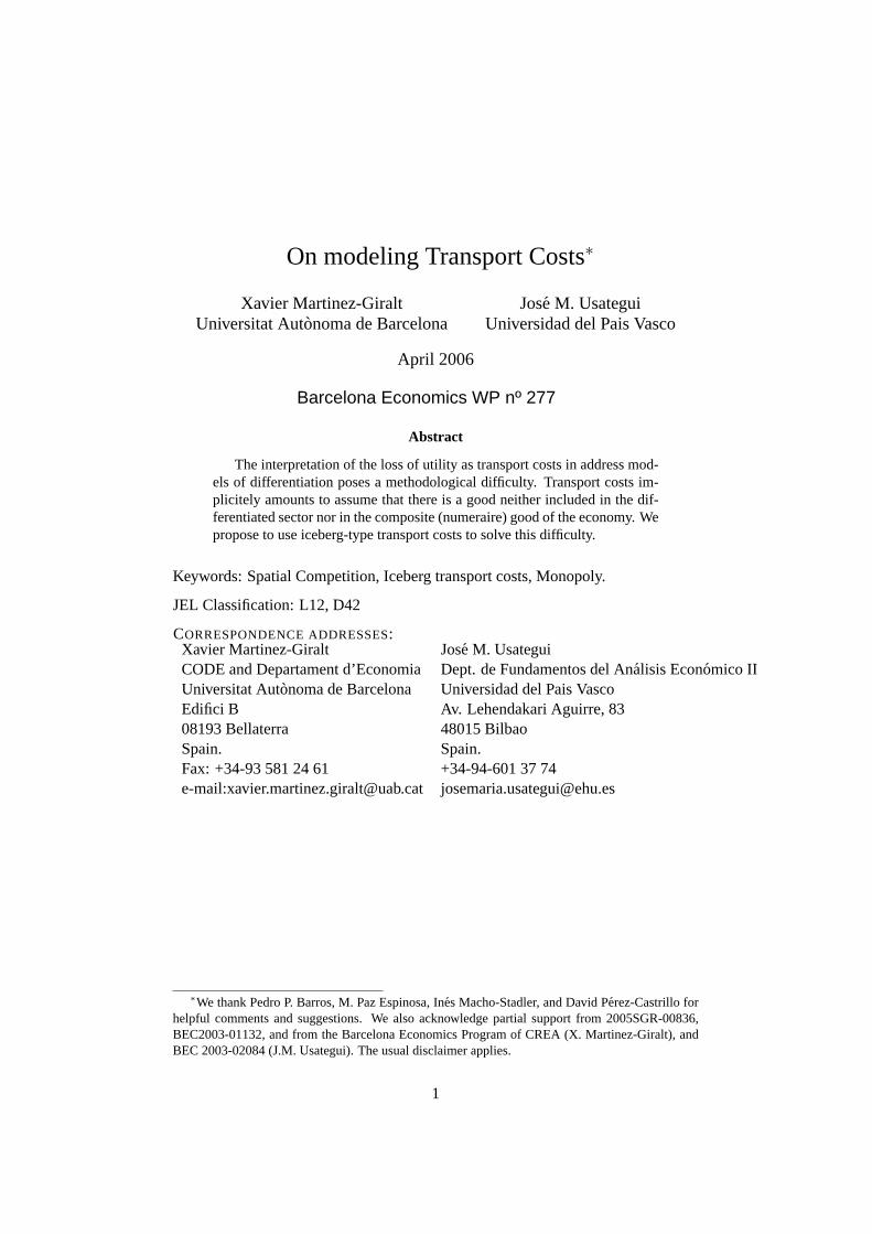
Figure 2: Firmi’s contingent demand.

Given the symmetry of the set up, we can focus on a generic firmi with demand

Di(pi, pj) = −2 + ea + e12−a

√pj

pi

Note that firmi’s market share will be positive if, givenpj its price is such that

the indifferent consumer is located atx(pi, pj) ≥ 0. That is, firmi will capture

some consumers whenever it quotes a pricepi ≤ pmaxi wherepmax

i is defined as

the solution ofx(pi, pj) = 0. Similarly, firm i will capture all the market when

quoting a pricepi ≤ pmini , wherepmin

i is the solution ofx(pi, pj) = 1. Formally,

pmaxi = epj , and pmin

i =pj

e.

Figure 2 represents firmi’s contingent demand. It is continuous, decreasing in

pi and convex in[pmini , pmax

i ].

Also, given p, and recalling that the price paid by a consumer located at a

distanceδ from the firm is given bypieδ, it follows thatpie

δ < p. As we assume

symmetric locations, it is necessary for firms to cover the market that,

pi <p

ea. (16)

From (12) and (16), and sinceea is increasing ina, it follows,

p

pi> max{e

12 , ea} = e

12 . (17)

9

4.2 Firms’ decision problem

Firms produce their differentiated variety with a constant returns to scale technol-

ogy, common to both firms and represented by a constant marginal costc > 0.

They aim at maximizing profits by choosing non-cooperatively their prices.

Firm i’s profits are given by,

Πi(pi, pj) = (pi − c)(−2 + ea + e

12−a

√pj

pi

)(18)

It is straightforward to compute,

∂Πi

∂pi= −2 + ea + e

12−a(pj

pi

) 12(pi + c

2pi

), (19)

∂2Πi

∂p2i

= −14e

12−ap

12j p− 5

2i (pi + 3c) < 0. (20)

Accordingly, firmi’s profit function is continuous and concave in[pmin, pmax].

From the inspection of the first order condition (19), it should be apparent that

this price game has a symmetric solution atpa = pb = p. Note also, that we

(implicitly) assumepi > c so that profits are well defined. In turn. this implies

from (17) that,p

c> e

12 , (21)

an expression that will be useful below.

4.3 Symmetric price equilibrium

The candidate symmetric price equilibrium (under full market coverage) of this

game is obtained from (19) after substitutingpi by p. It is given by,

p∗(a) =ce

12−a

4− 2ea − e12−a

. (22)

This candidate equilibrium price is well-defined only for some values of the loca-

tion parametera. In particular, note thatp∗(a) > 0 for a ∈ [0, 0.35), andp∗(a) < 0

for a ∈ (0.35, 0.5), and

lima→(0.35)−

p∗(a) = ∞, and lima→(0.35)+

p∗(a) = −∞.

10

Also, note thatp∗(a) is increasing and convex ina andp∗(0) > c. Thus,p∗(a) is

a candidate equilibrium price only ifa < 0.35. However, as we are characterizing

the equilibrium under full market coverage, we have to ensure that the most distant

consumer to the firm faces a price leaving him(her) indifferent between patronizing

the firm or staying out of the market. To identify such a price, recall that all con-

sumers have a reservation pricep. Also, the most distant consumer to, say, firma

is located at zero whena ≥ 1/4, and is located at 1/2 whena ≤ 1/4. Accord-

ingly, using (16), we obtain that the price at which the most distant consumer is

indifferent between buying and not buying is given by{pea if a ≥ 1

4p

e12−a

if a ≤ 14

(23)

From (22) and (23) we obtain that the symmetric price equilibrium under mar-

ket coverage is given by,

p∗ =

min{

ce12−a

4−2ea−e12−a

, pea , p

e12−a

}if a < 0.35

pea if a ≥ 0.35

(24)

That is, as long asp∗(a) is low enough to capture the most distant consumer, the

firm follows, whena < 0.35, the profit maximizing price. However, it may happen

that for a given location of the firm, the most distant consumer findsp∗(a) too high,

so that the full price of the purchase,p∗(a)eδ (with δ = max{a, (1

2 − a)}

), lies

above his(her) reservation price. Then, for those locations the firm will keep the

market covered charging the price given by (23). Hence,p∗ is defined as the lower

envelope of the prices given by (22) and (23).

Note that

Figure 3 summarizes the discussion. For anya ∈ [0, 12) the lower envelope is

characterized by the ratiop/c.

Four different configurations may arise. We can characterize them by com-

paring the values of the price functions ata = 0 and ata = 1/4. To ease the

11

1

2

1

4

.350

a

price

p

p!(0)

p

ea p

e1

2!a

p!(a)

p/e1

2

1

2

1

4

.350

a

price

p

p!(0)

p

ea p

e1

2!a

p!(a)

p/e1

2

a1 a2

1

2

1

4

.350

a

price

p

p

e1

2

p!(0)

p

ea p

e1

2!a

p!(a)

1

2

1

4

.350

a

price

p

p!(0)

p

ea p

e1

2!a

p!(a)

a

p/e1

2

a

(iv)p

c! 11.165

(i)p

c! 7.436 (ii)

p

c! (7.436, 7.742)

(iii)p

c! [7.742, 11.165)

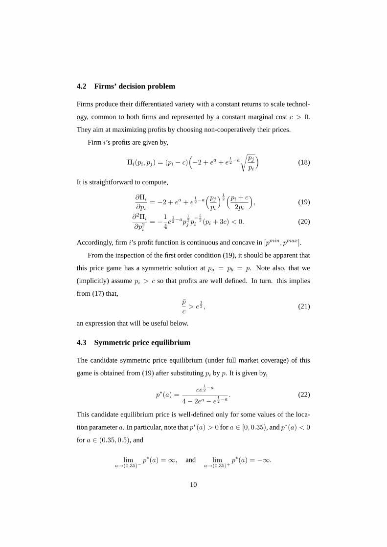
Figure 3: Symmetric equilibrium price profile

characterization, note that

p∗(0) =c

0.213, p∗(

14) =

c

0.115;

p

e12

=p

1.649,

p

e14

=p

1.284.

Accordingly,

p∗(0) >p

e12

⇐⇒ p

c< 7.742,

p∗(14) >

p

e14

⇐⇒ p

c< 11.165.

The four cases depicted in figure 3 are characterized by,

Case (i) is described byp∗(0) > p

e12

andp∗(14) > p

e14

. This implies pc < 7.742.

This bound is to be qualified by the argument of case (ii). There we argue

that the actual bound ispc ≤ 7.436. Also, in section 4.5 below, we will

identify a lower bound forpc given bye12 . Recalling (21), Case (i) can be

described bypc ∈ (e12 , 7.436].

12

Case (ii) is fairly subtle. The curvep∗(a) crosses the curve p

e12−a

twice. Note

that ∂p∗(a)∂a

∣∣∣a=0

= 0 < p

e12

=∂ p

e12−a

∂a

∣∣∣a=0

. Accordingly, it must be the

case thatp∗(0) > p

e12

. The subtlety of the argument appears when verifying

whether both crossings occur to the left ofa = 1/4, or the second crossing

occurs to the right ofa = 1/4. Let us consider this latter situation first. It

means thatp∗(14) < p

e14

. This implies pc < 7.742 and p

c > 11.165. Thus,

this case cannot arise, and it must be the case that both crossings happen

to the left ofa = 1/4. To see the intuition of this case, assume, for the

sake of the argument, thatp is fixed. Start with a high enough value ofc.

This places us in case (i) above. Now, lowering gradually the value ofc,

the curvep∗(a) shifts downwards. For some value ofc both curves,p∗(a)

and p

e12−a

will be tangent. Such tangency occurs where both slopes coincide,

yielding pc = 7.436. Therefore, case (ii) appears forp

c ∈ (7.436, 7.742), and

accordingly, case (i) as stated above is characterized bypc ≤ 7.436.

Case (iii) is described byp∗(0) < p

e12

andp∗(14) > p

e14

. Thus,pc ∈ (7.742, 11.165).

It is also easy to verify thatp∗(0) > c.

Case (iv) is described byp∗(0) < p

e12

andp∗(14) ≤ p

e14

. This impliespc ≥ 11.165.

Thus, we have a complete characterization of the symmetric price equilibrium of

the game, summarized in the following

Proposition 2. In a duopoly model with Samuelson melting, there is a symmetric

13

price equilibrium. It is characterized by

p∗ =

{p

e12−a

, for a ∈ [0, 14 ]

pea , for a ∈ [14 , 1

2 ]if p

c ∈ (e12 , 7.436]

p∗(a), for a ∈ [a1, a2]p

e12−a

, for a ∈ [0, a1] ∪ [a2,14 ]

pea , for a ∈ [14 , 1

2 ]

if pc ∈ (7.436, 7.742)

p∗(a), for a ∈ [0, a]

p

e12−a

, for a ∈ [a, 14 ]

pea , for a ∈ [14 , 1

2 ]

if pc ∈ [7.742, 11.165)

{p∗(a), for a ∈ [0, a]pea , for a ∈ [a, 1

2 ]if p

c ≥ 11.165

wherea1, a2 anda are the solutions ofp∗(a) = p

e12−a

in cases (ii) and (iii) respec-

tively, anda is the solution ofp∗(a) = pea in case (iv).

Note that givenpc , the equilibrium is unique. Also,p∗ is defined for alla ∈

[0, 12 ], and is continuous ina, but not necessarily differentiable in alla. Accord-

ingly, demand and profit functions are also continuous ina.

4.4 Location

To study the optimal (symmetric) location of the firm, recall that price equilibrium

is characterized, givenpc , by the lower envelope of the price functions,p∗(a), pea ,

and p

e12−a

.

We will proceed in two steps. First, we will study the behavior of the profit

function under each of the price functions. then we will characterize the equilib-

rium location according to the scenario induced bypc .

4.5 Study of the profit function Π(a)

Profits of the firm are defined, as usual, as the mark-up of the equilibrium price

over the (constant) marginal cost on the demand, that is,

Π(a) = (p∗ − c)D(a) = (p∗ − c)(−2 + ea + e12−a),

14

where we have made use of (14). We want to study the behavior of this profit

function with respect toa,

dΠ(a)da

=dp∗

daD(a) + (p∗ − c)

dD(a)da

,

d2Π(a)da2

=d2p∗

da2D(a) + 2

dp∗

da

dD(a)da

+ (p∗ − c)d2D(a)

da2,

wheredD(a)

da= ea − e

12−a,

d2D(a)da2

= ea + e12−a.

Lemma 1. Assumep∗ = pea . Then, the profit functionΠ(a) is decreasing ina.

Proof. Profits are defined fora ∈ (14 , 1

2) as,

Π(a) =( p

ea− c)(−2 + ea + e

12−a).

Note that (21) ensure that profits are well-defined. As

dp∗

da= − p

ea, and

d2p∗

da2= pea,

it follows,

dΠ(a)da

=1

e2a

[2p(ea − e

12

)− c(e3a − e

12+a)]

< 0

No general result can be obtained on the concavity or convexity of the profit func-

tion.

Lemma 2. Assumep∗ = p

e12−a

. Then, the profit functionΠ(a) is increasing ina.

Proof. Profits are defined fora ∈ (0, 14) as,

Π(a) =( p

e12−a− c)(−2 + ea + e

12−a),

Note that (21) ensure that profits are well-defined. As

dp∗

da=

d2p∗

da2=

p

e12−a

,

it follows,

dΠ(a)da

= ea− 12

[2p(ea − 1

)− c(e

12 − e1−2a

)]> 0

No general result can be obtained on the concavity or convexity of the profit func-

tion.

15

Lemma 3. Assumep∗ = ce12−a

4−2ea−e12−a

. Then,Π(a) has a minimum ata ≈ 0.05219266638

and is convex ina.

Proof. Profits are defined as,

Π(a) =( ce

12−a

4− 2ea − e12−a− c)(−2 + ea + e

12−a),

where

dp∗

da=

4ce12−a(ea − 1)(

4− 2ea − e12−a)2

d2p∗

da2=−4c

(4e

12−a − 6e

12 + e1−2a + 4e

12+a − 2e1−a

)(4− 2ea − e

12−a)3

Accordingly,

dΠ(a)da

= −2c(−2 + ea + e12−a)(6e

12−a − 3e

12 − 4ea + 2e2a − e1−2a)

(4− 2ea − e12−a)2

The first term in brackets in the numerator is always positive fora ∈ [0, 0.35]. The

second term in brackets has a root ata ≈ 0.05219266638, is positive for smaller

values ofa and negative for larger values ofa.

d2Π(a)da2

=2cΛ(a)

−(4− 2ea − e12−a)3

> 0,

becauseΛ(a) < 0 ∀a ∈ (0, 0.35), where

Λ(a) = 48e12−a + 24e3a + 12e

32−3a − 4e4a − e2−4a − 48e2a − 52e1−2a + 32ea

− 21e− 96e12 + 60e

12+a + 64e1−a − 12e

12+2a − 6e

32−2a

4.6 Location equilibrium

Once the behavior of the profit function has been fully identified, we can charac-

terize the (symmetric) location equilibrium of the game. For a given ratiopc , this

equilibrium is unique, as the following proposition states.

16

1

2

1

4

0a

profit

Figure 4: Location equilibrium forpc ∈ (e12 , 7.436)

Proposition 3. (i) Assumepc ∈ (e

12 , 11.165). Then, there is a symmetric loca-

tion equilibrium ata = 14 .

(ii) Assumepc ≥ 11.165. Then, there is a symmetric location equilibrium at

a = a, wherea is the solution ofp∗(a) = pea

Proof. See appendix

The intuition of the proposition goes as follows:

(i) Assumepc ∈ (e

12 , 7.436). From proposition 2, lemma 1 and lemma 2, the

profit function has the shape ahown in figure 4. Accordingly, the maximum

value of the profit function is reached ata = 14 . Note that at such point, the

profit function is not differentiable.

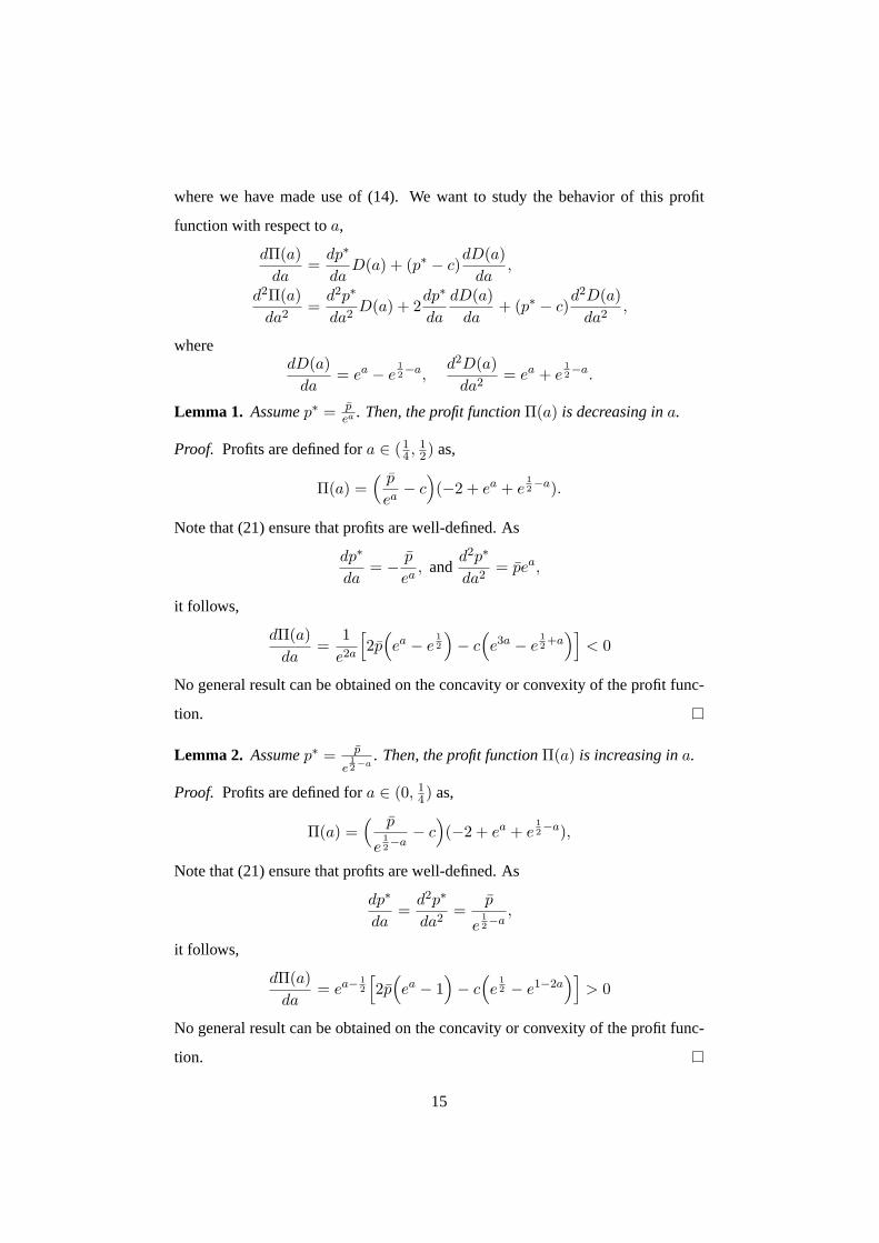
(ii) Assumepc ∈ (7.436, 7.742). From proposition 2, lemma 1, lemma 2, and

lemma 3, two possible scenarios illustrated in figure 5, may arise according

to the relative positions ofa1, a2 with respect to 0.052. Recall thata1 anda2

are the real solutions ofp∗(a) = p

e12−a

. Scenario 1 yields a unique maximum

at a = 14 . Scenario 2 shows two local maxima ata = a1 and ata = 1

4 . In

the appendix it is shown that the latter one is also a global equilibrium.

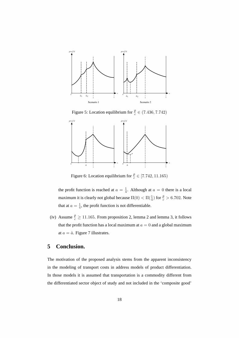
(iii) Assumepc ∈ [7.742, 11.165). From proposition 2, lemma 1, lemma 2, and

lemma 3, it follows that there are two possible shapes for the profit function

as shown in figure 6. In any of the two situations, the global maximum of

17

1

2

1

4

0a

profit

1

2

1

4

0a

profit

a1 a2 a1 a2

Scenario 1 Scenario 2

Figure 5: Location equilibrium forpc ∈ (7.436, 7.742)

1

2

1

4

0a

profit

a1

2

1

4

0a

profit

a

Figure 6: Location equilibrium forpc ∈ [7.742, 11.165)

the profit function is reached ata = 14 . Although ata = 0 there is a local

maximum it is clearly not global becauseΠ(0) < Π(14) for p

c > 6.702. Note

that ata = 14 , the profit function is not differentiable.

(iv) Assumepc ≥ 11.165. From proposition 2, lemma 2 and lemma 3, it follows

that the profit function has a local maximum ata = 0 and a global maximum

ata = a. Figure 7 illustrates.

5 Conclusion.

The motivation of the proposed analysis stems from the apparent inconsistency

in the modeling of transport costs in address models of product differentiation.

In those models it is assumed that transportation is a commodity different from

the differentiated sector object of study and not included in the ‘composite good’

18

1

2

1

4

0a

profit

a

Figure 7: Location equilibrium forpc ≥ 11.165

summarizing the rest of the economy. Methodologically, this is awkward because

transportation becomes an industry whose structure is not modeled. Who are the

agents or how transportation is provided is left unspecified. Curiously enough, this

way of modeling product differentiation is appealing because the intuitions derived

turn out to be quite useful.

We propose to solve this methodological inconsistency of the analysis by mea-

suring transportation in terms of the differentiated commodity, using the so-called

iceberg transport costtechnology introduced by Von Thunen in 1930 and formal-

ized by Samuelson in 1954. To our knowledge, this is the first attempt in the spatial

competition literature in proposing such an approach.

The iceberg formulation represents a new way of thinking in spatial competi-

tion. To make the reader familiar with it, we first illustrate its implications assum-

ing away all elements of competition. Next, we incorporate strategic interaction

with a simple symmetric duopoly model. We can characterize prize and location

competition in this new framework in terms of the ratio between the (common)

reservation price and the (constant and common) marginal production cost. Ac-

cording to this ratio, we can summarize symmetric equilibrium location decisions

in two patterns. Either firms locate at the first and third quartiles respectively, or at

points(a, 1− a), wherea ∈ (14 , 0.35).

19

References

Abdel-Rahman, H.M., (1994a), Economies of Scope in Intermediate Goods and aSystem of Cities,Regional Science and Urban Economics, 24, pp.497-524.

Abdel-Rahman, H.M., (1994b), Trade, Transportation Costs and System of Cities,mimeo.

Fujita, M., (1995), Increasing Returns and Economic Geography: Recent Ad-vances, mimeo.

Helpman, E. and P. Krugman, (1988),Market Structure and Foreign Trade, Cam-bridge, Mass, MIT Press.

Krugman, P., (1991), Increasing Returns and Economic Geography,Journal ofPolitical Economy, 99(3), pp. 483-499.

Krugman, P., (1992), A Dynamic Spatial Model, NBER, working paper No. 4219.

Samuelson, P.A. (1983), Thunen at Two Hundred,American Economic Review,vol. XXI, pp. 1468-1488.

Thunen, J.H. von, 1930,Der Isolierte Staat in Beziehung auf Landwirtschaft undNationalokonomie, third ed., Ed. Heinrich Waentig, Jena: Gustav Fisher(english translation Peter Hall (ed.)von Thunen’s Isolated State, London,Pergamon Press, 1966.)

Appendix: Proof of Corollary 1

i) Under MQD melting we have:

∂h(δ, µ)∂δ

=µ

(1− µδ)2

and

H(δ, µ) =1µ

(−µδ − ln(1− µδ)).

Hence,

(1 + h(a, µ))2 =1

(1− µa)2

and∂h(a, µ)

∂δ(a + H(a, µ)−H(0, µ)) =

− ln(1− µa)(1− µa)2

.

As ln(1− µa) < 0 andd ln(1− µa)

da< 0, if expression (8) in Proposition 1

holds fora = L2 , it will also hold fora < L

2 .

20

Given that

1(1− µL

2 )2>− ln(1− µL

2 )(1− µL

2 )2⇔ e >

11− µL

2

⇔ 2e− 1eµ

> L,

we obtain, from Proposition 1, the result.

ii) Under MD melting we have:

∂h(δ, µ)∂δ

= µαδα−1

and

H(δ, µ) =µδα+1

α + 1.

Hence, as

(1 + h(a, µ))2 = 1 + 2µaα + µ2a2α

and

∂h(a, µ)∂δ

(a + H(a, µ)−H(0, µ)) = αµaα +α

α + 1µ2a2α,

the inequality (8) in Proposition 1 holds forα ≤ 2. Accordingly, forα ≤ 2

the monopolist locates at the center and covers all the market.

iii) Under Samuelson melting we have:

∂h(δ, µ)∂δ

= µeµδ

and

H(δ, µ) =eµδ

µ− δ.

Hence, given that

(1 + h(a, µ))2 = e2µa

and∂h(a, µ)

∂δ.(a + H(a, µ)−H(0, µ)) = e2µa − eµa,

from Proposition 1 we obtain that the monopolist locates at the center and

covers all the market.�

21

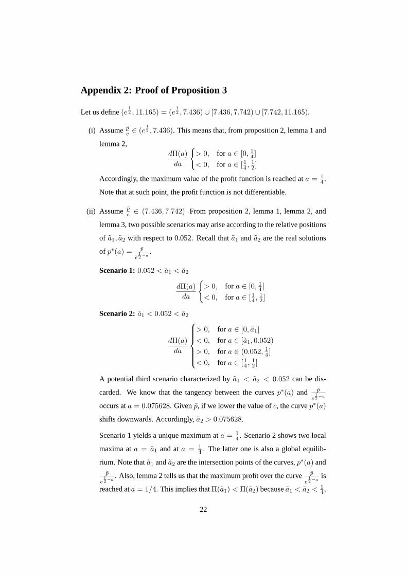
Appendix 2: Proof of Proposition 3

Let us define(e12 , 11.165) = (e

12 , 7.436) ∪ [7.436, 7.742) ∪ [7.742, 11.165).

(i) Assumepc ∈ (e

12 , 7.436). This means that, from proposition 2, lemma 1 and

lemma 2,dΠ(a)

da

{> 0, for a ∈ [0, 1

4 ]< 0, for a ∈ [14 , 1

2 ]

Accordingly, the maximum value of the profit function is reached ata = 14 .

Note that at such point, the profit function is not differentiable.

(ii) Assumepc ∈ (7.436, 7.742). From proposition 2, lemma 1, lemma 2, and

lemma 3, two possible scenarios may arise according to the relative positions

of a1, a2 with respect to 0.052. Recall thata1 anda2 are the real solutions

of p∗(a) = p

e12−a

.

Scenario 1:0.052 < a1 < a2

dΠ(a)da

{> 0, for a ∈ [0, 1

4 ]< 0, for a ∈ [14 , 1

2 ]

Scenario 2: a1 < 0.052 < a2

dΠ(a)da

> 0, for a ∈ [0, a1]< 0, for a ∈ [a1, 0.052)> 0, for a ∈ (0.052, 1

4 ]< 0, for a ∈ [14 , 1

2 ]

A potential third scenario characterized bya1 < a2 < 0.052 can be dis-

carded. We know that the tangency between the curvesp∗(a) and p

e12−a

occurs ata = 0.075628. Givenp, if we lower the value ofc, the curvep∗(a)

shifts downwards. Accordingly,a2 > 0.075628.

Scenario 1 yields a unique maximum ata = 14 . Scenario 2 shows two local

maxima ata = a1 and ata = 14 . The latter one is also a global equilib-

rium. Note thata1 anda2 are the intersection points of the curves,p∗(a) andp

e12−a

. Also, lemma 2 tells us that the maximum profit over the curvepe

12−a

is

reached ata = 1/4. This implies thatΠ(a1) < Π(a2) becausea1 < a2 < 14 .

22

(iii) Assumepc ∈ [7.742, 11.165). From proposition 2, lemma 1, lemma 2, and

lemma 3, it follows that

dΠ(a)da

< 0, for

{a ∈ [0, 0.052] if a > 0.052a ∈ [0, a] if a < 0.052

> 0, for

{a ∈ [0.052, 1

4 ] if a > 0.052a ∈ [a, 1

4 ] if a < 0.052< 0, for a ∈ [14 , 1

2 ]

In any of the two situations, the maximum value of the profit function is

reached ata = 14 . Although ata = 0 there is a local maximum it is clearly

not global becauseΠ(0) < Π(14) for p

c > 6.702. Note that ata = 14 , the

profit function is not differentiable.

(iv) Assumepc ≥ 11.165. From proposition 2, lemma 2 and lemma 3, it follows

that

dΠ(a)da

< 0, for a ∈ [0, 0.0522)> 0, for a ∈ (00522, a]< 0, for a ∈ [a, 1

2 ]

Accordingly, the maximum value of the profit function is reached ata = a.

As in (iii) here we find again a local maximum ata = 0. HoweverΠ(0) <

Π(a) because( c

0.213− c)(−2 + 1 + e

12 ) <

( p

ea− c)(−2 + ea + e

12−a)

wherep

ea=

ce12−a

4− 2ea − e12−a

,

can be simplified to

(−2 + ea + e12−a)2

4− 2ea − e12−a

> 1.198

The fraction on the left-hand side is increasing and convex ina ∈ (14 , 0.35).

Therefore, it has a minimum value of

(−2 + e14 + e

14 )2

4− 2e14 − e

14

= 2.181.

Hence, it follows that the profit function reaches its global maximum ata =

a. Note that at such point, the profit function is not differentiable.�

23