Centre de Referència en Economia Analítica

Barcelona Economics Working Paper Series

Working Paper nº 246

Testing for Adverse Selection into Private Medical Insurance

Pau Olivella and Marcos Vera-Hernández

January19, 2006

Testing for Adverse Selection into PrivateMedical Insurance∗

Pau Olivella† and Marcos Vera-Hernández‡

January 19, 2006

Abstract

We develop a test for adverse selection and use it to examine pri-vate health insurance markets. In contrast to earlier papers that con-sider a purely private system or a system in which private insurancesupplements a public system, we focus our attention on a system whereprivately funded health care is substitutive of the publicly funded one.Using a model of competition among insurers, we generate predictionsabout the correlation between risk and the probability of taking pri-vate insurance under both symmetric information and adverse selec-tion. These predictions constitute the basis for our adverse selectiontest. The theoretical model is also useful to conclude that the settingthat we focus on is especially attractive to test for adverse selection.Using the British Household Panel Survey, we find evidence that ad-verse selection is present in this market.

∗We are grateful for useful comments from Jerome Adda, James Bank, Richard Blun-dell, Simon Burgess, Winnand Emmons, Emla Fitzsimons, Matilde Machado, Carol Prop-per, Lise Rochaix-Ranson, and other participants at seminars in Bristol, University CollegeLondon, as well as the European Health Economics Workshop in Oslo, International Indus-trial Organization Conference in Chicago, the International Health Economics AssociationConference in Barcelona, and the ASSET meeting in Ankara. All remaining errors are ouronly responsibility. Vera acknowledges financial support by a Marie Curie Fellowship ofthe European Community program, Improving Human Research Potential and the Socio-economic Knowledge Base, under contract no. HPMF-CT-01206. Olivella acknowledgesfinancial support from the Departament d’Universitats, Recerca i Societat de la Informació,Generalitat de Catalunya, projects 2001SGR-00162 and 2005SGR00836; as well as fromPrograma Nacional de Promoción General del Conocimiento, project BEC2003-01132, andthe Barcelona Economics Progamme of CREA.

†Department of Economics and CODE, Universitat Autònoma de Barcelona, 08193Bellaterra, Spain; E-mail: pau.olivella@uab.es

‡University College London, and Institute for Fiscal Studies. E-mail: m.vera@ucl.ac.uk

1

Barcelona Economics WP nº 246

JEL: D82 I19 G22Key Words: Contract theory, Testing, Health Insurance

1 Introduction

Although adverse selection is one of the main assumptions of contract theory,

empirical papers find mixed evidence of its existence. Yet the existence of

adverse selection is important because it is one of the main justifications for

public intervention in areas such as insurance markets (Dalbhy, 1981).

In this paper we test for the existence of adverse selection in health insur-

ance markets in a framework where a public health administration finances

health care in full through income taxes and where individuals with private

insurance may resort to an alternative source of care. In other words, pri-

vately funded and publicly funded care are, de facto, mutually exclusive; we

refer to this setting as the “substitutes framework,” and test propositions

from a theoretical model that incorporates the features of this framework.

This distinction is important because the competitive equilibrium that arises

within this framework has, to our knowledge, never been studied under either

symmetric information or adverse selection. Previous literature has focused

either on a “supplements framework,” where the private insurance is supple-

mental to the public one, or on one where the public insurance is absent,

which we call a “purely private framework.”

As our theoretical model shows, the consequences of adverse selection

are more dramatic in our framework than in the other two. Consequently,

our institutional setting is better suited to test for the existence of adverse

selection. Our theoretical model also shows that, as far as the test of adverse

selection is concerned, the supplements framework and the purely private

framework yield similar predictions.

To apply these frameworks to a few real world examples, in the US, a large

2

segment of the population is not eligible for either Medicaid or Medicare and

must resort to private insurance. Hence, this is an example of a purely

private framework. In France and Belgium, as well as for the part of the

population covered by Medicare in the US, an individual obtains a basic

insurance contract from the insurer of his choice and receives funding from

the government to cover this basic coverage. In addition, the individual can

buy a supplementary contract to cover whatever copayments and services

are not covered by the basic contract. Hence these are examples of the

supplements framework. Finally, in the UK, Spain, Italy, and many other

European countries, the public insurance system provides treatment instead

of just financing some basic coverage. Moreover, except for prescriptions and

dental care, copayments in the public system are nil so there is no room to

supplement the public coverage. Instead, an individual can only substitute

the public coverage by receiving care funded through private insurance.

Consistent with the above discussion, we perform a test of adverse selec-

tion in the UK, a substitutes framework (Besley and Coate 1991). Everyone

is publicly insured through the British National Health Service (NHS). The

NHS is, in turn, financed through taxation. Hence individuals contribute to

the financing of public care whether they use it or not. It may seem a puzzle

why, in such a system, anyone would purchase private insurance in the first

place. The reason is that enrollees are able to obtain treatment from the

private sector without having to put up with long waiting lists (Besley and

Coate, 1991; Propper and Maynard, 1989). Health care obtained through

private insurance also offers better ancillary services.

The contributions of this paper are two-fold. First, we solve a theoret-

ical model of competition among insurers under the substitutes framework.

We compare the equilibrium set of contracts and choices under symmetric

information with those under adverse selection. In order to draw compar-

isons, we also briefly recall the equilibrium contracts under the supplements

3

and purely private framework. For each setting, we adapt and extend the

perfectly competitive paradigm developed by Rothschild and Stiglitz (1976).

As a second contribution, we test for adverse selection in the UK. To our

knowledge, this is the first time such a test has been carried out under a

substitutes framework. In this sense, our theoretical contribution is key for

our empirical test, as we need to know the equilibrium features under the

substitutes framework to be able to test for adverse selection there.

According to our theoretical results, under the substitutes framework

and under adverse selection, high-risk individuals are the ones who purchase

private insurance. In contrast, under this framework and in the absence

of adverse selection, low-risk individuals are the ones who purchase private

insurance. In other words, under the substitutes framework the sign of the

correlation between the probability of purchasing private insurance and risk

is positive in the presence of adverse selection and negative in its absence.

This stands in clear contrast to what occurs under the supplements frame-

work, where all individuals have a strong incentive to purchase private in-

surance regardless of their risk and regardless of the presence or absence of

adverse selection. In other words, under the supplements framework there is

absolutely no correlation between enjoying private insurance and risk. This

does not mean, of course, that no test can be performed under this frame-

work. Our theoretical model shows (and this is not new) that, under adverse

selection, high-risk individuals tend to purchase more coverage. That is, un-

der adverse selection a positive correlation between risk and coverage should

be observed. In the absence of adverse selection, all individuals purchase

high coverage contracts in equilibrium, hence there is no correlation between

risk and coverage.

Notice that there are two differences between the substitutes and the

supplements frameworks. First, the test under the latter must be based on

observations on each individual’s coverage, whereas in the former, it suffices

4

to observe whether private insurance is purchased or not. Second, in a sup-

plements framework, we need to distinguish a positive correlation from zero

correlation, while in a substitutes framework we need to distinguish a positive

correlation from a negative one. This gives more power to our test.

We test for adverse selection using the British Household Panel Survey.

Our test compares the probabilities of hospitalization of employees who re-

ceive private medical insurance as a fringe benefit, and those who buy it

directly. Since the benefits offered by corporate policies are very similar

to those offered by individually purchased policies (Propper and Maynard,

1989) both groups will have the same access conditions to hospitalization.

Consequently, any positive difference in the probabilities of hospitalization

between the two groups is due to differences in risk.

We find that individuals who purchase medical insurance have a higher

probability of hospitalization than individuals who receive private medical

insurance as a fringe benefit. This constitutes evidence in favour of the

presence of adverse selection in the English private medical insurance market.

Our test could be biased if individuals in worse health status tend to be

employed in jobs with employer-provided medical insurance. However, if

this bias were present, it could only reinforce the empirical results found.

One could also argue that our findings could be due to heterogeneity in the

benefits provided by employer-provided and individually purchased medical

insurance. We use the same dataset to rule out this possibility.

Let us briefly review the theoretical literature on adverse selection where

private health insurance coexists with the public system. In the supplements

framework, the Medigap system in the US (supplemental to Medicare) has

received the most attention. Gouveia (1997) studies the political outcome on

a model of supplementary private health insurance in the absence of adverse

selection. Feldman et al. (1998) study the equilibrium under adverse selec-

tion. Delipalla and O’Donnell (1999) combine the two previous papers in a

5

supplementary private health insurance market.

As for the substitutes framework, the general approach in the literature

on the substitutive public provision of private goods (such as health care

or education) has focused on its role as a redistributive device. A seminal

paper here is the one by Besley and Coate (1991), who propose the NHS

in the UK as an example of a substitutes framework. Blomquist and Chris-

tiansen (1998) study when governments should implement supplementary

rather than substitutive systems.1 In contrast to them, we do not aim to

analyze the redistributive role of the substitutive system, rather we focus

on how informational assumptions of health risk heterogeneity influence the

equilibrium.

The literature on empirical testing of adverse selection has recently gained

attention. On the one hand, some works cast doubts on the presence of

adverse selection. For example, in his review, Chiappori (2000) concludes

that the importance of adverse selection is limited. Cardon and Hendel (2001)

do not find evidence of adverse selection in the US employer-provided health

insurance market either. Chiappori and Salanie (2000) find no evidence of

adverse selection in the automobile insurance market. In the life insurance

market, neither Cawley and Philipson (1999) nor Hendel and Lizzeri (2003)

find evidence of adverse selection.

On the other hand, Ettner (1997) finds evidence of adverse selection in

the Medicare market in the US and Gardiol et al. (2005) provides evidence of

adverse selection in a strongly regulated private insurance market in Switzer-

land. Abbring et al. (2003) discuss econometric approaches to distinguish

between adverse selection andmoral hazard. Cohen and Einav (2005) develop

a structural econometric model that allows for unobserved heterogeneity in

both the probability of accident and risk aversion. Although some of their

results could be indicative of adverse selection, the authors recognize that

1See also this paper for a literature review on publicly provided private goods.

6

they cannot separetely identify moral hazard from adverse selection. Finkel-

stein and Poterba (2004) find evidence of adverse selection in the UK annuity

market. It is clear that more research is needed to obtain a better assessment

of the presence of adverse selection in insurance markets.2

As for the UK, our testing arena, several papers have investigated the

determinants of private medical insurance (King andMossialos 2002, Propper

et al. 2001, Besley et al. 1999, Besley et al. 1998, Propper 1993, Propper

1989). These papers highlight the role of political ideology, quality, resources

available to the private sector, insurance premiums and income. However, to

our knowledge, adverse selection has not been investigated in this particular

market.

Our paper is organized as follows. In Section 2 we introduce the model of

the substitutes framework. In Section 3 we study the equilibrium under this

framework. We do this under symmetric information in subsection 3.1 and

under adverse selection in subsection 3.2. In Section 4 we study the equilib-

rium under the supplements framework and discuss what a test of adverse

selection should be in this setting, and we compare it with the substitutes

framework. In Section 5 we perform the empirical analysis. In subsection 5.1

we describe the data. In subsection 5.2 we explain the test in detail, and in

subsection 5.3 we report our main results and show a sensitivity analysis. In

Section 6 we conclude the paper. The proofs of all lemmata and propositions

are in Appendix A. The definition of the variables and descriptive statistics

are in Appendix B.

2Cameron et al. (1988), Coulson et al. (1995), Vera-Hernández (1999) and Schellhorn(2001) focus on estimating how coverage influences health care use while controlling for theendogeneity of insurance coverage, i.e., for adverse selection. As a subproduct, it is tempt-ing to interpret the results of the endogeneity test as evidence of asymmetric information.However, as Chiappori (2000) emphasizes this approach is likely to overestimate adverseselection substantially, as most specification errors will give evidence of endogeneity evenin the absence of adverse selection.

7

2 The model

We start by describing our main framework, the substitutes framework. Two

features distinguish this framework: (i) If an individual with private insur-

ance falls ill, he must choose between the private treatment covered by his

insurance and the public treatment. He cannot have an operation in the

public sector and then receive its postoperative treatment in a private hos-

pital. Private and public services cannot be combined. (ii) When a privately

insured individual chooses the private treatment, the private insurer must

bear the full cost of treatment. These two features rule out supplementary

private health coverage, i.e., insurance to cover the copayments borne by the

individual when treated in the public sector.3

All individuals in the economy are obliged to pay income taxes, which are

dedicated to finance public sector expenditures, including public health care.

This care is provided by a set of providers that are either public or have been

subcontracted by the NHS.4 We refer to this set as PUB henceforth.

We study the game that starts once (i) the health authority (HA hence-

forth) has chosen and committed to a specific package of services that is

provided free of charge, and (ii) the individual has already paid his personal

income taxes, which contribute to the financing of the PUB. An important

but realistic assumption is that all individuals in a given observable class

(say women of a certain age) receive the same treatment, rather than being

3In the UK, a substitutes framework, the public insurance only charges copaymentsfor outpatient drugs, vision tests, and dental treatment. These copayments are quitelow. For instance, individuals only pay out-of-pocket £6.5 (US$ 11.50) for each out-of-pocket drug prescribed. Charges for dental treatment and vision tests are also small (seehttp://www.dh.gov.uk/assetRoot/04/10/69/10/04106910.pdf). In fact, as far as we areaware, all the countries under the substitutes framework have very low copayments fora limited set of services. Most services covered by the public insurer are free of charge.Consequently, there is no room for private insurers to supplement the copayments thatthe public insurer charges.

4The subcontracted providers may be private, public-private consortia, or not-for-profitfoundations. However, since they have signed contracts with the NHS to treat NHS pa-tients, we still refer to them as public providers.

8

offered a menu of options.

In this game there are two sets of players, a large set of private insurance

companies (insurers henceforth) that compete for individuals, and a large

number of individuals, where each can be one of two types (described below).

The first movers are the insurers, who take into account the option that

individuals can resort to the PUB set of providers for free. The insurers

simultaneously choose the package of services that will be delivered in case

of illness and also the premium that consumers must pay before knowing

whether or not they will become ill. We assume that insurers as well as the

HA condition their offers to each observable class of individuals. We therefore

perform all of our analysis for a single and prespecified class.

The second and last movers are the individuals. Once they have learned

their probability of becoming ill (i.e., their type) but before they know

whether or not they will actually become ill, they simultaneously decide

whether to purchase private insurance and, if so, from which insurer. Con-

ceptually, each individual first looks at the best contract for him and then

compares it with the public package.

The assumption that insurers take the public package of services as given

can be justified as follows. The quality, waiting time, copayment regime, and

so on at the PUB is determined by the HA’s budget, which is the result of

a lengthy political process. In contrast, insurers make these decisions more

flexibly. The assumption is also convenient because it allows us to leave aside

the way in which the HA’s budget is decided, as well as the objective function

of whomever decides this budget (e.g., the government or the parliament).

If an individual has chosen to purchase private insurance from a specific

insurer, he enjoys double coverage. If this individual falls ill, he chooses

between two options associated with two distinct sets of providers, the set

PUB and the set of providers that are offered by his insurer, which we call

PRI. The sets PUB and PRI may imply different copayments, waiting times,

9

qualities, ancillary services, or protocols. We will measure all of these charac-

teristics, as well as the initial health status, in monetary units, as is standard

in models of insurance under adverse selection.5

We denote by 0 the loss suffered by an individual who is not treated

at all and has fallen ill. We can describe an insurer’s offer, henceforth "con-

tract," by a two-dimensional vector ( PRI , q), where PRI denotes the insurer’s

commitment to reduce the insuree’s final losses from 0 to PRI if he seeks

treatment through the set PRI, and q denotes the insurance premium.

If an individual obtains treatment from the set PUB (either because he

has not purchased private insurance or because he prefers the public treat-

ment), his loss is reduced to PUB. Notice that the public package consti-

tutes an outside option for an individual who has not yet decided whether

to purchase private insurance. This outside option can also be described as

a two-dimensional vector ( PUB, 0), where the second component is zero be-

cause taxes paid are independent of whether private insurance is purchased

or not.6 We refer to this option as “the public package,” henceforth. It is

important to note that private contracts where PRI > PUB are irrelevant

as they are dominated by the public package.

Finally, notice that an ill consumer could also choose to go untreated even

5In some models of health insurance in the absence of adverse selection, individualshave preferences (often additively separable) over disposable income and health. See, forinstance, Gouveia (1997). Our analysis is simpler in this dimension.

6An implicit assumption is that an agent does not receive a tax rebate if he chooses topurchase private insurance. In the presence of a tax rebate, if an agent decides to purchaseprivate insurance, the government returns part of the taxes paid by this consumer. Sincewe will be drawing the analysis in the final wealth space, the position of the zero isoprofitconstraint associated with attracting a given type depends on this tax rebate. We can,however, prove that our results do not change if the tax rebate is proportional to thepremium paid. More specifically, one can show that this is equivalent to a simultaneouschange in the exogenous probability of illness for each type. If, on the other hand, thetax rebate were a fixed constant, then our theoretical results would have to be revised.Nevertheless, such fixed rebates are not usually observed. As for our testing arena, arebate was in place for individuals over age 60 in the UK prior to the July 1997 budget,but this rebate was proportional to the premium.

10

though public treatment is free. We rule out this possibility by assuming that

0 ≥ PUB, that is, public treatment does reduce the losses suffered by an ill

individual. We solve the game by backward induction.

We are now ready to describe the players’ payoffs. At the point in time

(τ , for expositional simplicity) when the individual must decide whether or

not to purchase private insurance he does not know if, at time τ 0 > τ , he will

become ill. At point in time τ the individual initial position is measured by a

single parameter w, which includes his health status as well as his disposable

wealth, i.e., net of taxes. We refer to this parameter as initial wealth.

Suppose that the individual has purchased some private insurance con-

tract ( PRI , q). As noted before, this means that PRI < PUB. If the individ-

ual does not become ill, he enjoys final wealth w − q. If he does become ill,

he enjoys final wealth w− q− PRI . In contrast, suppose that the individual

has not taken private insurance. If he does not fall ill he enjoys final wealth

equal to w. Otherwise, since we have assumed that 0 > PUB, he obtains

public treatment from PUB and hence enjoys final wealth equal to w− PUB.

There are two types of individuals, low risks and high risks. Low-risk

individuals may suffer an illness with probability pL. High-risk individuals

may suffer the same illness with probability pH . Of course, 0 < pL < pH < 1.

The individual’s probability of illness is publicly observable under symmetric

information, and is only observed by him under asymmetric information.

We analyze both the symmetric and the asymmetric information cases. It

is common knowledge that the proportion of low risks in the economy is

0 < γ < 1. We denote by p = γpL + (1 − γ)pH the average probability of

illness in the population. This parameter will play an important role below.

All individuals have the same utility function u over final wealth, with u0 > 0

and u00 < 0.

An individual who may suffer an illness with probability p and who de-

cides not to purchase private insurance enjoys expected utility pu(w− PUB)+

11

(1−p)u(w). If he does purchase some private contract ( PRI , q), his expected

utility is pu(w − PRI − q) + (1− p)u(w − q).

Insurers are risk neutral. Suppose that an insurer S has attracted an

individual i of type J ∈ {L,H} with a contract ( , q). Suppose that i fallsill. Then S must bear the costs of ensuring that i does not suffer a loss larger

than , as promised in the contract. Since we are under the substitutes

framework, these costs must be borne in full by the insurer. Since losses in

the lack of treatment are 0, the insurer in fact bears the cost of reducing

losses from 0 to . We simplify the analysis by assuming that each dollar of

loss reduction costs the insurer exactly one dollar. This yields linear isoprofit

lines, as it is standard in insurance models. The expected profits of offering

( , q) are therefore given by q − pJ( 0 − ).

It is perhaps clarifying to discuss here the main difference between the

substitutes and the supplements frameworks. Under the supplements frame-

work, the only costs that the insurer would bear when committing to a loss

of are the costs of reducing losses from PUB to so that expected profits

would be given by q − pJ( PUB − ).

We now perform a change of variable to conduct the standard graphical

analysis in the space of final wealths. Suppose an individual has purchased

a private insurance contract ( , q). His final wealth in case of illness is given

by a = w − − q (a for ”accident”). In case of no illness, it is given by

n = w − q (n for ”no accident”). It is easy to check that q = w − n and

= n− a. Hence, an insurer attracting a J-risk with a final-wealth contract

(n, a) expects to obtain

ΠJ(n, a) = q − pJ( 0 − ) = w − n− pJ( 0 − n+ a). (1)

Isoprofits have slope da/dn = −(1− pJ)/pJ . It is easy to check that the

zero isoprofit goes through the point of neither private nor public insurance,

given by (n, a) = (w,w − 0) and denoted by A. The zero isoprofits are

12

depicted in Figure 1 and labeled ΠJ(·) = 0 for J = L,H.

Notice that in the presence of the public package, the status-quo point

of an individual is not A but (w,w − PUB). This is the final wealth vector

associated with the public package and we denote this point as P . In Figure

1, each point in the vertical line through n = w is a possible position of P .

As PUB decreases (or as public coverage increases), P lies at a higher point

in this vertical line. If PUB = 0, we are back to the no-insurance point A.

By virtue of the change of variable performed above, an individual’s ex-

pected utility is given by UJ(n, a) = pJu(a)+(1−pJ)u(n). His marginal rateof substitution between states is given by

da

dn−

∂UJ (n,a)∂n

∂UJ (n,a)∂a

= −1− pJpJ

u(n)

u(a).

In Figure 1 we depict one indifference curve for each type. The slope

of an indifference curve at the 45-degree line is −1−pJpJ, and coincides with

the slope of the corresponding isoprofit. Therefore efficiency is attained for

any contract in the 45 degree line. This corresponds to contracts with full

coverage, where n = a, or = 0.

The presence of the public package P at the outset (i.e., constituting a

committed offer) may imply that some contracts that were attracting indi-

viduals in the equilibrium in the absence of P may now become inviable, and

vice versa. Hence the following terminology.

Definition 1 If a contract α attracts some individuals we say that the con-

tract is active. Analogously, if the public package P attracts some individuals

we say that the public sector is active.

A sufficient condition for a contract to be active in equilibrium is that it

offers strictly more utility to some risk type than both the rest of the con-

tracts offered and the public package. The same goes for the public package.

13

However, this condition is not necessary. If some type is indifferent between

two offers, both offers may attract individuals of this type. Anyhow, the only

tie-breaking rule that we need to solve the model is the following.

Assumption 1 If all individuals of type J are indifferent between the public

package P and the best private contract for them, all individuals of type J

choose the public package.7

Our equilibrium notion is the following.

Definition 2 An equilibrium set of active contracts S (ESAC henceforth)

is a set of contracts (that may or may not include the public package P ) such

that

(i) Each and every contract in S is offered either by some insurer(s) or by

the public sector and is active.

(ii) If a single insurer deviates by offering a contract outside this set, either

this contract will be inactive or this insurer will not make additional profits.

3 The substitutes framework

We solve first the game under the hypothesis of symmetric information. We

then proceed to the case where health risks are an individual’s private infor-

mation. Finally, we compare the equilibria in the two settings.

3.1 The game under symmetric information

The low-risk and the high-risk markets are segmented. Consider first the

situation where there is no public system. We know from Rothschild-Stiglitz

(1976) that the competitive equilibrium entails efficient contracts (full in-

surance) and zero profit per individual no matter his type. Therefore, for

7Assuming that some agents do choose the private sector out of indifference would notgreatly change our results.

14

all J = L,H; we have nJ = aJ and ΠJ(n, a) = 0, which implies, using

(1), that w − aJ − pJ 0 = 0, or aJ = nJ = w − pJ 0. This yields con-

tracts {α∗H , α∗L} = {(w − pH 0, w − pH 0), (w − pL 0, w − pL 0)}, which aredepicted in Figure 1.

We now find the ESAC for each possible P . We illustrate our arguments

by means of Figure 1. Point H0 is the public package (n, a) = (w,w −PUB) such that a high risk is indifferent between α∗H and H0. Point L0 is

the public package such that a low risk is indifferent between α∗L and L0.

The following lemma cannot be proven graphically and is a consequence of

Jensen’s inequality.8

Lemma 1 H0 < L0.

Once the positions of H0 and L0 are known, we can analyze the situation

case by case, i.e., for each possible position of P . In Case 1, P lies below

point H0; in Case 2, P coincides with H0; in Case 3, P lies strictly between

point L0 and pointH0; in Case 4, P coincides with L0; in Case 5, P lies above

L0. For each case, we find the ESAC. This yields the following proposition.

Proposition 1 Suppose that adverse selection is absent. Then, under as-

sumption 1, a unique ESAC exists for each and every position of the public

package P , and is characterized as follows.

a) In Case 1, the ESAC is {α∗L, α∗H}, high risks pick α∗H, and low risks pickα∗L; the public sector is inactive.

b) In Cases 2 and 3, the ESAC is {α∗L, P}, low risks pick α∗L, and high riskspick P .

c) In Cases 4 and 5, the ESAC is {P} and only the public sector is active.

8We are indepted to Juan Enrique Martínez-Legaz for providing the elegant proof thatcan be found in the Appendix.

15

Notice that the only cases where both sectors are active are 2 and 3,

where only the low risks resort to the private sector. This yields the following

corollary.

Corollary 1 Suppose that the two sectors are active and adverse selection

is absent. Under assumption 1, the probability of illness among the privately

insured is pL, which is smaller than p, the average in the general population.

The reason we compare the probability of illness of those who purchase

insurance with the average probability in the general population will be ex-

plained in Section 5, since it is relevant for our empirical test.

3.2 The game under adverse selection

As in the previous section, consider first the situation where there is no public

health system. We know from Rothschild-Stiglitz (1976) that the competitive

equilibrium, if it exists, entails an efficient contract (full insurance) for the

high risks and zero profits for an insurer attracting a high risk. Therefore,

the high risk contract under asymmetric information is the same as under

symmetric information, α∗H . The low-risk contract must satisfy the high-risk

incentive compatibility constraint with equality and also yield zero profits.

These two equations yield the contract depicted by α̂L in Figure 2.

As it is well known, this set of contracts {α̂L, α∗H} constitutes only a can-

didate, albeit unique, for a competitive equilibrium. Recall that in the purely

private competitive model there exists a critical γ (γ∗ henceforth), such that

an equilibrium exists if and only if γ ≤ γ∗. This γ∗ is the proportion of low

risks such that the zero-isoprofit line associated to pooling contracts (not

depicted) is tangent to the indifference curve bUL in Figure 2. If γ > γ∗ then

a lens appears between this isoprofit line and curve bUL. Any contract in the

interior of the lens pools both risks, but makes positive profits on average,

16

thus constituting a profitable deviation from the candidate. We will prove

later that the condition for existence in the purely private market also en-

sures existence of an equilibrium once we introduce the public sector. Hence

we introduce it here.

Assumption 2 The proportion γ of low risks in the population is less than

or equal to the critical proportion γ∗ for existence in the purely private frame-

work.

Using the set of contracts {α̂L, α∗H} that is active in the equilibrium in

the absence of a public package, we can divide the possible positions of the

public contract P into five cases, as in the previous section. In Figure 2, point

H0 is again the public contract such that a high risk is indifferent between

α∗H and H0. Notice that point H0 is the same whether adverse selection is

present or not, since the equilibrium contract for the high risk is the same.

Point L1 is the public contract such that a low risk is indifferent between α̂L

and L1. The relative position of H0 and L1 is given in the next lemma.

Lemma 2 H0 > L1.

We are now ready to establish the five possible cases that one has to

deal with when characterizing the competitive equilibrium. In Case 1, P lies

below point L1; in Case 2, P coincides with L1; in Case 3, P lies strictly

between point L1 and point H0; in Case 4, P coincides with H0; in Case 5,

P lies above H0. For each case, we find the ESAC. This yields the following

proposition:

Proposition 2 Suppose that adverse selection is present. Then, under as-

sumptions 1 and 2, a unique ESAC exists for each and every position of the

17

public package P , and is characterized as follows.

a) In Case 1, the ESAC is {α̂L, α∗H}, high risks pick α∗H, and low risks pick

α̂L; the public sector is inactive.

b) In Cases 2 and 3, the ESAC is {α∗H , P}, low risks pick P , and high riskspick α∗H.

c) In Case 3, assumption 2 is no longer necessary for existence of a compet-

itive equilibrium.

d) In Cases 4 and 5, the ESAC is {P} and only the public sector is active.

The proof follows the usual arguments used in the purely private model.

However, they have to be modified because the committed presence of the

public package offer must be taken into account. Perhaps the only instance

where this presents some difficulty is the following. Some deviations that

are not profitable in the purely private model because they violate incentive

compatibility may become profitable in the presence of P . The idea is that

the public package may absorb the high-risk individuals who otherwise would

have flocked to the deviation. We prove that this cannot be true in Cases

1, 2, and 3 because P is not attractive enough, while in Cases 4 and 5 the

private sector is not active in the first place.

Notice that both sectors are active in cases 2 and 3 only. We have the

following and most important corollary.

Corollary 2 Suppose that the two sectors are active and adverse selection

is present. Then, under assumptions 1 and 2, the probability of illness for

those who decide to purchase private insurance is pH, which is larger than p,

the average in the general population.

Again, the reason we compare the probability of illness of those who

purchase private insurance with the average probability in the population

18

will be explained in Section 5. In any case, notice that corollaries 1 and 2 tell

us that the sign of the difference between p and the probability of illness of

the privately insured crucially depends on the presence of adverse selection.

This stands in clear contrast with the results that we obtain in the next

section, where we explore the supplements framework.

4 Comparisons with the Supplements frame-work

The underlying model of supplementary private insurance is quite different

from the one with substitutive insurance. The HA commits beforehand to a

specific level of loss reduction, say 0− PUB. If the individual has purchased

private insurance, he enjoys a further reduction in loss, say PUB − 0. Most

importantly, the private insurer bears the cost of only this last loss reduction.

This is the key distinction with the substitutes framework, where the insurer

bears the full cost of reducing the loss from 0 to 0. To sum up, under

the supplements framework, the expected profit of an insurer committing to

a final loss equal to 0 < ˆ is given by (1− pJ) q + pJ (q − ( PUB − 0)) =

q − pJ ( PUB − 0).

We conduct the same change of variable as in the previous section. For

an individual who has purchased private insurance, we have a = w − q − 0

and n = w − q. Then q = w − n and 0 = n− a. Therefore, expected profit

is given by w − (1− pJ)n− pJ (a+ PUB). We next find the location of the

zero-isoprofit line in the space (n, a). Notice that if 0 = PUB (zero private

coverage) then q = 0 as well. Then a = w − PUB and n = w, i.e., the

status quo of the individual without private insurance who resorts to public

treatment. The slope of any isoprofit is given by

da

dn= −

∂ΠJ (n,a)∂n

∂ΠJ (n,a)∂a

= −1− pJpJ

,

19

as before. Hence, this model is equivalent to the classic Rothschild-Stiglitz

model except that the status quo point is (n, a) = (w,w − PUB) instead of

(n, a) = (w,w − 0). Hence, Figure 2 can be used to depict the compet-

itive equilibrium under both symmetric information and adverse selection

by replacing the vertical intercept for point A shown there (i.e., w − 0)

with w − PUB.9 The competitive equilibrium without adverse selection is

given by (α∗L, α∗H), whereas the equilibrium under adverse selection is given

by (α̂L, α∗H). Note that if an individual does not purchase private insur-

ance, then his final wealth pair is at point A, which is clearly inferior for

both types of individuals under both symmetric and asymmetric informa-

tion. This yields the most important result here. That is, regardless of the

presence or absence of adverse selection, all types would, in principle, take

private insurance. Hence the average probability of illness in the private sec-

tor would always be equal to p. Having purchased private insurance or not

cannot be an explanatory variable for differences in risk.

In order to obtain a test for adverse selection in the supplements frame-

work, one needs to observe the particular private contract that each indi-

vidual enjoys in the sample chosen. The model then predicts that in the

absence of adverse selection all individuals take full coverage. Among those

with full coverage, the average probability of falling ill is p, the same as in

the general population. If, on the other hand, adverse selection is present,

then the model predicts that low risks will enjoy lower coverage than high

risks. Hence, those who choose to purchase full coverage have a higher prob-

ability of requiring treatment than the average probability in the population.

9This does not mean that the position of the isoprofit lines remains intact after theintroduction of public insurance. Only the construction of the competitive equilibriumremains the same. In particular, by introducing public insurance in such a way thatprivate insurance becomes supplemental (a supplements framework), the status quo pointA not only changes its vertical position but also its horizontal one. This is because initialincome w includes taxes, and these will surely change if the public coverage is to befinanced through income taxation.

20

The methodological difference between this test and the one we propose is

discussed at the end of subsection 5.2.

5 Empirical test for adverse selection

In the UK, everyone is entitled to free treatment under the public sector.

However, the losses borne in case of illness are quite large because waiting

times are long for hospital stays, for elective surgery, and for consultation

with a specialist.10 Private insurance, in contrast, allows individuals to ob-

tain hospitalization services with negligible waiting time. These institutional

features are shared with other countries with a substitute system, for in-

stance Spain. In relation to our theoretical model, individuals with private

insurance suffer from a smaller loss than individuals with only public insur-

ance. This indicates that our testing ground satisfies a feature of our model,

namely, active insurers must be offering larger loss reductions than the public

option.

5.1 The data

In this paper we use the British Household Panel Survey (BHPS). The BHPS

is an annual survey designed as a nationally representative sample of house-

holds. All individuals in respondent households become part of the longitu-

dinal sample. The same individuals are interviewed again in successive years;

the survey retains those individuals who split from existing households in the

sample by including the new households that they form.

We will restrict our sample to waves 6 to 12 of the BHPS. These waves

correspond to data collected between August 1996 and April 2003. The pre-

vious waves do not have information on employer-provided health insurance.

10Other causes of high loss in the public system are a restricted choice of specialists andpoor ancillary services.

21

We will consider only the case of employees who have private medical insur-

ance in their own names because it is the only instance in which we know

who pays for the private medical insurance. We will focus on England, which

accounts for 62% of the BHPS sample for the waves that we use. The samples

of Scotland, Wales, and Northern Ireland are quite small for the 6th, 7th,

and 8th waves of the panel. Moreover, the percentage of individuals with

private medical insurance varies substantially across these four nations. The

percentage of individuals with private medical insurance is 18% in England,

while it varies between 10% and 12% in the others. In addition, the organi-

zation of the NHS can vary substantially across these four nations. Thus, we

focus our estimation on England. The definition of the variables and their

descriptive statistics for the sample used in the estimation can be found in

Table B1 in Appendix B.

5.2 The test

In the UK, public and private insurance coexist. In the terminology of our

theoretical section, both sectors are active. According to our theoretical

model (corollary 2), if adverse selection is present then the probability of

privately insured individuals requiring medical care is higher than the aver-

age in the population. Conversely, in the absence of adverse selection, the

probability of requiring medical care of the privately insured is lower than

the average in the population, see corollary 1. In sum, our theoretical model

predicts that in a substitutes framework, such as the UK, adverse selection

has a drastic effect on the sign of the difference between the average probabil-

ity of requiring medical care and this probability for those who decide to buy

private health insurance. The sign of this difference will depend on whether

or not adverse selection is present. Moreover the difference will never be zero

in equilibrium. This makes our institutional framework attractive for testing

for adverse selection.

22

Therefore, one could build a test for adverse selection by comparing the

risk of requiring medical care of those who decided to buy private medical

insurance with the risk of those who decided not to buy it. However, one does

not observe whether an individual truly requires medical care but whether

an individual actually uses health care services. Hence, we use actual uti-

lization as a proxy for requiring medical care. Unfortunately, this proxy may

suffer from an upward bias. Individuals with private health insurance might

be hospitalized more often than individuals without private health insurance

because they enjoy better access conditions (e.g., less waiting time) and not

because they have a higher probability of requiring medical care. We correct

this bias by comparing two groups of individuals with the same access condi-

tions to hospitalization. To this end, we will test for adverse selection using

only people who are privately insured.

In the UK, there are three ways to acquire private insurance. First, pri-

vate medical insurance can be bought directly in the market by the individ-

ual. Second, some employers offer their employees the option to buy private

medical insurance. If the employee decides to buy the insurance offered by

his employer, he will have the premium deducted explicitly from his wage.

Consequently, he might decide not to buy it. However, most employees will

decide to buy it because the premium will tend to be lower than if he buys

the insurance directly. Third, and very importantly for us, some employers

directly provide their employees with private medical insurance as a fringe

benefit.11 The BHPS asks about the source of private health insurance only

for individuals who have health insurance in their own name. According to

the BHPS, privately insured employees obtain their private insurance as fol-

lows: 43.7% pay directly for it, 12% have the insurance deducted from their

11We cannot rule out the possibility that an employee could approach his employerasking for an increase in wages in exchange of not enjoying the fringe benefit. However,this would only attenuate the results that we find.

23

wages, and 44.3% get it from the employer as a fringe benefit.

Our test for adverse selection will compare the probability of hospitaliza-

tion of those who purchase private medical insurance directly with those who

receive it as a fringe benefit from their employer.12 Individuals that have the

insurance deducted from their wages pay the private medical insurance in

total. However, as the purchase is arranged through the company, the insur-

ance premium might be particularly low. Consequently, they do not face the

same prices as the group of individuals who buy private medical insurance

directly. That is why we exclude them from our analysis.13

According to Propper and Maynard (1989, p.11), the benefits offered by

corporate policies are very similar to those offered by individually purchased

policies. This is very important for our test, as this means that both groups

will face the same access conditions to hospitalization. We will discuss this

further at the end of this section. Notice that our results on the presence

of adverse selection will only be valid for the employee population. In order

to extend the homogeneity of the comparison groups even further, we will

restrict the sample to individuals who are employed on a permanent basis.

Our identification assumption is that, conditional on covariates and be-

ing permanently employed, having employer-provided health insurance is in-

dependent of health status. As a consequence, the group with employer-

provided health insurance has a probability of hospitalization equal to the

average probability of hospitalization in the population of employed indi-

viduals with permanent jobs. This assumption is, of course, conditional on

covariates that we will include in the model as education, age, gender, and

income.

Two types of selection issues could potentially invalidate our identifica-

12We choose hospitalizations because in the UK private medical insurance is mainlyused for hospital treatment.13The results are very similar when we include them and we use a dummy variable for

their category.

24

tion assumption, and therefore bias our results. One type of selection is

“employer driven” and the other one is “employee driven.” The first one is

related to the fact that some jobs are more likely to offer employer-provided

health insurance than others. According to Tables 1 and 2, the percentage of

employees with employer-provided health insurance differ considerably by in-

dustry and type of occupation.14 For instance, managers and administrators

are more likely to enjoy employer-provided health insurance than clericals

workers. Financial services are also more likely to enjoy employer-provided

health insurance than the agriculture sector. An employer-driven bias could

potentially emerge if the health characteristics of employees of certain in-

dustries or occupations tend to be different from the average, conditional on

covariates. However, in order to be sure that this will not bias our results,

we include industry and occupation among our set of covariates.

[TABLES 1 AND 2 AROUND HERE]

Another possible source of bias in our comparison could be an “employee

driven” bias. This would be the case if employees in worse health status look

for jobs that offer employer-provided health insurance. Our source of data

offers some evidence against such behavior. The BHPS asks individuals who

changed jobs what was the main reason why they did so. The survey specifies

sixteen possible reasons, as well as the option “other”. Most individuals

answered “more money,” or “better promotion prospects.” However, the

option of health insurance was not given in the list of 16 possible reasons.

Nonetheless, only 7.6% of the individuals chose “other.” In any case, as

we will discuss later, even if this source of bias were present, it would only

attenuate the effect that we find.15

14The percentages in the table are for employees who have health insurance in their ownname because it is for this group that we know who pays their health insurance.15Ettner (1997) already gave this argument in the US context.

25

We believe that our identification assumption is credible for the reasons

mentioned above. A similar identification assumption has been maintained

for the US by Ettner (1997) and Cardon and Hendel (2001).16 We believe

that this assumption is more likely to hold in the UK than in the US. The

provision of health insurance by the employer should be less important in

the UK than in the US because the NHS is available free to anyone in the

UK, and individuals cannot opt out of it.

The logic of the test we perform is that the population of employed indi-

viduals with permanent jobs is split into two groups: those who must decide

whether to buy private insurance or not (or group D, for “deciders”) and

those who receive private medical insurance from their employer as a fringe

benefit (or group N, for “non deciders”). As we previously justified it, our

assumption is that, conditional on covariates, this division can be considered

independent with respect to the risk of requiring hospitalization. Conse-

quently, both groups have a probability of hospitalization that is equal to

the population average conditioned on covariates. Now, group D can again

be divided into two subgroups: those who purchase private insurance, or

group D1, and those who do not, or group D2. Since individuals in group D

decide whether or not to buy private medical insurance, their behavior will

follow our model of a substitutes framework (Section 3). Consequently, if

adverse selection is present, the probability of hospitalization in group D1

should be higher than the population average, i.e., that in group N. Con-

versely, in the absence of adverse selection, the probability of hospitalization

in group D1 should be lower than in group N.

Notice that if the difference in the probability of hospitalization were

not significantly different from zero then the only possible conclusion would

16Chiappori and Salanie (2003) state in page 129 that “the main identifying assumptionused by Cardon and Hendel is that agents do not choose their employer on the basis ofthe health insurance coverage.”

26

be that the data are not informative enough to reject the null hypothesis

that information is symmetric. It could not mean that adverse selection is

absent, since if this were the case then the difference in the probability of

hospitalization would not be zero but negative. This is strikingly different

from the tests performed under the supplement or fully private framework

where a non significant correlation between health care use and insurance

coverage is taken as evidence against the presence of adverse selection.

5.3 Results

We will use a probit model to estimate the difference in the probability

of hospitalization between groups N and D1. We prefer to use a standard

probit model rather than a random effect probit model to avoid making

distributional assumptions on the individual random effect. The estimates of

the standard error are adjusted to take into account that the same individual

is observed in different waves. The variable IND takes value 1 when the

individual pays directly for the private medical insurance and takes value

0 otherwise.17 The omitted category is formed by individuals that receive

private medical insurance as a fringe benefit. The key coefficient for our

test is the one corresponding to IND that will drive the difference in the

probability of hospitalization between groups N and D1.

The results are reported in Table 3. We first focus on the second and

third columns where dummies for occupation and industry are not included

as covariates. The table shows that the estimates of income and education

are not significantly different from zero. According to these results, it is not

easy to find variables that predict the probability of hospitalization. This

suggests that adverse selection could be important since insurers will also find

17As we mentioned before, we exclude from the analysis those individuals whose insur-ance premium is explicitly deducted from their wage. The results do not change if weinclude them and we use a different binary variable for them.

27

it difficult to predict this probability. Regarding our formal test for adverse

selection, we find that individuals who buy private medical insurance directly

have a higher probability of hospitalization than individuals whose provides

private medical insurance as a fringe benefit. The difference in probability

of hospitalization when covariates are fixed at their average value is 0.021.

This is a large difference given that the average probability of hospitalization

in the sample is 0.064. This constitutes clear evidence of adverse selection in

the English private medical insurance market.

As a robustness test of our results, we estimate the same model for hos-

pitalizations as before but include the dummies for occupations and industry

that are given in Tables 1 and 2. As mentioned before, we do this be-

cause the probabilities of having employer-provided health insurance differ

significantly by industry and occupation, so that an “employer driven” bias

could be present in the absence of these dummies. The results in the fourth

and fifth columns show that the dummies for industry and occupation are

not jointly significant. Consequently, the rest of the results hardly change.

We still find a statistically significant difference in the probability of hos-

pitalization between those who purchased health insurance and those with

employer-provided health insurance. The difference in probability of hospi-

talization when covariates are fixed at their average value is 0.020 for this

specification.

[TABLE 3 AROUND HERE]

Above we have found that the probability of hospitalization is larger

for group D1 individuals than for group N individuals. We interpret this as

evidence of adverse selection, as we have assumed that individually purchased

policies are as generous as corporate policies. Our assumption is in line

with existing information about the private insurance market in England

(Propper and Maynard, 1989, p.11). However, an alternative explanation

28

of our empirical findings is that individually purchased policies are more

generous than corporate policies. In what follows, we will argue that this

alternative explanation is not supported by data. Recall first that individuals

with private medical insurance are still eligible to be covered by the NHS.

Whether they will choose to be treated by the NHS or by private insurance

will depend on the waiting time in the NHS and the generosity of their private

coverage policy (deductibles, maximum amount covered, illnesses excluded,

covered treatments, and so on). If individually purchased policies were more

generous than corporate policies, then we should observe that, conditional on

having a hospitalization, the probability of choosing NHS-funded treatment

is smaller for individuals in the D1 group than for individuals in the N group.

We test this hypothesis using data from the BHPS.18 In Table 4, the estimate

of the coefficient of IND is not statistically different from zero at 95% of

confidence. This shows that there is no statistically significant difference in

the probability of choosing NHS coverage between group D1 and group N.

Consequently, the hypothesis that individually purchased policies are more

generous than corporate policies lacks empirical support. Though the sample

size is relatively small, the sign of the coefficient is positive rather than

negative. If anything, this could indicate that corporate policies are more

generous than individually purchased ones. If that were true, we would be

underestimating the presence of adverse selection. Our results in Table 4

are in line with Propper and Maynard (1989), who claim that the benefits

provided by corporate and individually purchased insurance policies are very

similar.

[TABLE 4 AROUND HERE]

Finally, we address another robustness feature of our analysis. Before we

18There are 15 individuals that declare that their treatment was only partially fundedby the NHS. We included them as if they did not choose NHS funded treatment.

29

assumed that individuals would not consider whether the employer-provided

private medical insurance when deciding whether to accept their current job.

It is important to mention that if this assumption were false in reality then

the most likely bias would lead us to underestimate adverse selection. If

anything, those in worse health status would be more likely to join group N

(i.e., wait until they are offered jobs that include private medical insurance

as a fringe benefit). This would mean that group N is less healthy than

the average employee. Our data indicate that individuals who have bought

medical insurance directly (group D1) are in a worse health status than

individuals in group N. Therefore, if the bias were present then the difference

in health status between group D1 and the average employee which indicates

adverse selection would in fact be larger than the difference that we have

estimated.

6 Conclusions

Recent empirical literature has found mixed support for the presence of ad-

verse selection. In this paper, we focus on an institutional framework that

has not been exploited before to test for adverse selection. In particular,

we focus on a NHS framework where privately and publicly funded care are

substitutive. Using a theoretical model, we have derived the properties of

the equilibria in the presence and in the absence of adverse selection. The

nature of the equilibria depends on the generosity of the public coverage. In

the interesting case in which public and private markets coexist, we show

that the probability of requiring medical care for individuals with private

health insurance is higher than the average in the population in the presence

of adverse selection. Conversely, in its absence, the probability of requir-

ing medical care for those with private health insurance is smaller than the

average in the population. Hence, our model predicts that in a substitutes

30

framework like the NHS, adverse selection has a dramatic effect on the sign of

the difference between the average probability of requiring medical care and

the average probability for those who decide to buy private health insurance.

The sign of this difference will depend on whether or not adverse selection

is present. Moreover the difference will never be zero in equilibrium. This

makes our institutional framework an attractive one for an adverse selection

test.

In England, private medical insurance is mostly used for hospitalizations.

We test for adverse selection by comparing the probabilities of hospitalization

of permanent employees that receive private medical insurance as a fringe

benefit, and those who buy it directly. We find strong evidence of adverse

selection in the English private medical insurance market. Our test could be

biased if individuals in worse health status tend to be employed in jobs with

employer-provided medical insurance. However, if this bias were present, it

could only attenuate the evidence of adverse selection.

7 Appendix A

Proof of Lemma 1

Let H0 = (w, aH) and L0 = (w, aL). We need to prove that aH < aL, or

equivalently that u(aH) < u(aL). Now H0 satisfies UH(w, aH) = UH(α∗H).

This implies pHu(aH) + (1− pH)u(w) = u(w − pH 0). Similarly, L0 satisfies

UL(w, aL) = UL(α∗L). This implies pLu(aL) + (1 − pL)u(w) = u(w − pL 0).

Solving for u(aH) and u(aL), we need to prove that

u(aH) =u(w − pH 0)− (1− pH)u(w)

pH<

u(w − pL 0)− (1− pL)u(w)

pL= u(aL).

31

After some manipulation, this can be rewritten as

u(w − pL 0) >pLpH

u(w − pH 0) + u(w)pH − pL

pH. (2)

Let x1 = w−pH 0, x2 = w, p1 =pLpH, and p2 =

pH−pLpH

. Notice that 0 < p1 < 1,

0 < p2 < 1, p1+p2 = 1; so that (p1, p2) is a system of probabilities. Let Ep(·)be the expectation operator associated to these probabilities. Notice that

Ep(x) ≡ p1x1 + p2x2 = w − pL . Therefore, expression (2) can be rewritten

as

u(Ep(x)) > Ep(u(x)).

This is true by Jensen’s inequality and the fact that u(·) is strictly concave.

Proof of Proposition 1

Step 1. We prove first that no contract outside the set {P,α∗L, α∗H} can be-long to an ESAC. In other words, any ESACmust be a subset of {P, α∗L, α∗H}.Under symmetric information, the private market is segmented. Fix a type

J = L,H. Suppose, by contradiction, that in equilibrium the private sec-

tor attracts some individuals of type J with contract α0 6= α∗J . Then

UJ(α0) > UJ(P ) and moreover either α0 does not yield zero profits or is

not efficient, since if both were false then efficiency and zero profit would im-

ply that α0 = α∗J . Take the first case, where profits are positive. Then there

exists ε > 0 such that α0 = α0+ε

·11

¸and UJ(α

0) > UJ(α0) ≥ UJ(P ), so α0

monopolizes all individuals of type J and still makes positive profits per con-

sumer if ε is small enough, contradiction. Suppose now that α0 is not efficient,

then there exists another contract α0 such that UJ(α0) > UJ(α0) ≥ UJ(P )

and ΠJ(α0) > ΠJ(α0) (and α0 monopolizes all individuals of type J), contra-

diction.

Step 2. We now prove the proposition on a case-by-case basis.

Proof of part (a). Suppose that P is below H0 in Figure 1. We prove first

that {α∗L, α∗H} is indeed an ESAC. Suppose that α∗J is offered in exclusivity

32

to type J individuals, which is possible since types are publicly observable

here. Since UJ(α∗J) > UJ(P ) for all J , we have that both α∗L and α∗H are

active. If any other contract is offered by an insurer with exclusivity to some

type J , this contract will either attract no one or will result in losses, by

construction of α∗J . We prove now that no other ESAC exists. By step 1

any ESAC must be a subset of {P, α∗L, α∗H}. Consider {P, α∗L, α∗H}. Noticethat P is inactive, which violates condition (i) of the definition of an ESAC.

Consider {P,α∗J} for some J . Again P is inactive. Consider {P}. Since Plies below the indifference curve going through α∗J , ∀J , we have that, for εsmall enough, an insurer offering α0 = α∗J − ε

·11

¸with exclusivity for type

J makes positive profits.

Proof of part (b). Suppose that P is on or above point H0 but below point

L0 in Figure 1. We start by proving that {P, α∗L} is an ESAC. Supposean insurer offers a contract with exclusivity for high risks. By assumption

1, to attract high risks it must lie strictly above the high-risk indifference

curve UH∗. By construction such a contract will result in losses. Suppose

an insurer deviates by offering a contract with exclusivity for low risks. To

attract low risks it must lie on or above curve UL∗. No such contract will

make positive profits. We now prove that {P, α∗L} is the only ESAC. NoESAC may contain α∗H , because all low risks prefer P to α∗H and high risks

choose P out of indifference by assumption 1. Then by Step 1 an ESAC

must be a subset of {P, α∗L}. Consider {P}. Since P lies below L0, we have

that, for ε small enough, an insurer offering α0 = α∗L−ε·11

¸makes positive

profits. Consider {α∗L}. If insurers offer α∗L with exclusivity to low risks, highrisks will be attracted by P , so it should belong to the ESAC, contradiction.

If insurers offer α∗L to the whole population, then also high risks will pick

this contract, and hence insurers will suffer losses. The only other possible

subset is the same {P, α∗L}, and we are done.Proof of part (c). Suppose that P is on or above L0. To see that {P} is

33

an ESAC, notice that any private offer that attracts individuals of any type

will suffer losses. To see that {P} is the only ESAC, pick any other set ofcontracts. Since P is an outstanding offer, neither α∗L nor α

∗H can be active.

By Step 1 we are done.

Proof of Lemma 2

This lemma is a straightforward consequence of the single-crossing condition.

The proof is therefore omitted.

Proof of Proposition 2

A few statements are proved as preliminary steps.

Step 1. If the private sector attracts any individual at all in equilibrium, it

must do so at zero average profit per individual.

Suppose by contradiction that the ESAC S includes a contract α offered

by the private sector that makes profits Πα > 0 per individual. Since the

premise is that it is active, it must attract individuals with types in some

set T and be rejected by the rest of types, i.e., in the complement of T (TC

henceforth) which could be empty, as in the case where α is pooling. In other

words,

(i) For all J ∈ T , we have UJ(α) ≥ UJ(α0) for all α0 ∈ S ∪ {P}.(ii) For all J ∈ TC, we have UJ(α) ≤ UJ(α0) for some α0 ∈ S ∪ {P}.Due to the single-crossing condition, there is always a deviating contract

β arbitrarily close to α that

(iii) will be preferred to α by all types in T , i.e., UJ(β) > UJ(α) for all

J ∈ T ;

(iv) will be dispreferred to α by all types in TC , i.e., UJ(β) < UJ(α) for

all J ∈ TC;

so we can write

(i’) for all J ∈ T , we have UJ(β) > UJ(α0) for all α0 ∈ S ∪ {P};

34

(ii’) for all J ∈ TC, we have UJ(β) < UJ(α0) for some α0 ∈ S ∪ {P}.To sum up, β will attract and repel the same types of individuals as contract

α, but will monopolize all the individuals of any type in T . Since β can

be made arbitrarily close to α, we find that profits per individual Πβ are

arbitrarily close to Πα (by continuity), whereas the number of individuals

attracted is multiplied due to monopolization. Thus β constitutes a profitable

deviation from S.

Step 2. If the private sector attracts some high risks and no low risks in

equilibrium through some contract α, this contract must be efficient.

We already proved that it should yield zero profits. Suppose by contradiction

that contract α is not efficient but attracts high risks in equilibrium. Then

UJ(α) ≥ UJ(α0) for all α0 ∈ S ∪ {P}. Since α is not efficient, there existsanother contract β that yields higher profits and attracts all high risks and

may or may not attract low risks. In both cases (since low risks have a lower

probability of illness), β constitutes a profitable deviation.

Step 3. There does not exist an equilibrium where the private sector attracts

both individuals through a single contract α.

Recall first that such a contract would have to make zero profits on average

per individual. Moreover, by assumption 1 it must be true that UJ(α) >

UJ(P ) for all J . Due to the single-crossing condition, a contract β always

exists that is preferred to α by low risks and at the same time it is dispreferred

to α by high risks. Therefore β will also be preferred to P by low risks, while

high risks stick to α. Hence β constitutes a profitable deviation.

Step 4. In equilibrium, if a contract attracts type J only, it must yield zero

profits per client.

By Step 1 we know that if α is active, on average it must make zero profits.

Now suppose that it makes positive profits per low risk and negative profits

per high risk. Then this contract must be a pooling one. By step 3 this can

never be part of an equilibrium.

35

Step 5. If the private sector attracts high risks, it must be through contract

α∗H.

This follows directly from steps (4) and (2).

We turn now to characterizing the competitive equilibrium, case by case.

The proof is based on Figure 2.

Case 1. P lies below point L1

We prove first that {α̂L, α∗H} is indeed an ESAC in the presence of such

package P . We must prove that it cannot be the case that a deviation

from {α̂L, α∗H} that was unprofitable in the absence of P ("before") becomes

profitable once P is present ("now"). This could only happen in the following

ways.

1.1 The deviation did not attract any consumers before and now it not

only attracts consumers but also does so in a profitable way.

1.2 The deviation did attract some high risks, but in an unprofitable way,

whereas now it still attracts them but now become profitable.

1.3. The deviation did attract some low risks, but in an unprofitable way,

whereas now it still attracts them but now become profitable.

1.4. The deviation did attract both risks, but in an unprofitable way,

whereas now it only attracts low risks, thus making the deviation profitable.

We now prove that none of these statements is possible. Statement 1.1

is impossible because if a contract β did not attract anyone in the absence

of P , the presence of this alternative cannot make consumers more willing

to accept α0 contract β. Statements 1.2 and 1.3 are impossible because the

per-client profits of attracting a given risk are independent of the existence

of an alternative contract P . Statement 1.4 requires that

(i) package P attracts the high risks that otherwise would have picked β,

i.e., UH(P ) ≥ UH(β);

(ii) contract β attracts some or all low risks, i.e., UL(β) ≥Max{UL(α̂L), UL(P )};

36

(iii) contract β is profitable when it attracts a low risk, i.e., ΠL(β) > 0.

Now (i) and (ii) imply UH(P ) ≥ UH(β) ≥ UL(P ). The single-crossing

condition implies that β is on or to the right of the vertical line going through

A (autarky) and P . Also, (ii) and (iii) imply that UL(β) ≥ UL(α̂L) and

ΠL(β) > 0. By inspection of Figure 2, this implies that β lies in the lens

formed by isoprofit ΠL(·) = 0 and indifference curve bUL. This lens is strictly

to the left of the vertical line going through A, which leads to a contradiction.

Let us now prove that {α̂L, α∗H} is the unique ESAC in the presence of

P . We begin by showing that P cannot belong to an ESAC. Suppose it

does. If it attracts high risks, all other contracts in the ESAC must lie below

the high-risk indifference curve going through P , UHP henceforth. Since P

lies below L1, curve UHP and isoprofit ΠH(·) = 0 form a lens. Any deviation

in the interior of the lens will attract high risks and bring positive profits,

contradiction. As a corollary, the private sector must be attracting the high

risks. By step 5 this implies that the private sector is offering α∗H . Suppose

now that P attracts low risks. Then, again since P is on the vertical line

through w and below L1, we find that an area appears between the low-risk

indifference curve going through P , the indifference curve UH∗, and isoprofit

ΠL(·) = 0. Any contract in this area is preferred to P by low risks, it is

dispreferred to α∗H by high risks, and it makes positive profits per low risk,

so it constitutes a profitable deviation.

Finally, since only the private sector is active and we have already shown

that the high risks must be attracted by α∗H , then the only other incentive

compatible contract αL that attracts low risks and yields zero profits must

lie on the segment α̂LA. If it coincides with α̂L, we are done. If is strictly

below, an area appears between the low-risk indifference curve going through

αL, the indifference curve UH∗, and isoprofit ΠL(·) = 0. Any contract in thisarea constitutes a profitable deviation, and we are done. This proves part

(a) of the proposition.

37

Cases 2 and 3. P coincides with or is above point L1 but below H0.

We prove first that {P,α∗H} is indeed an ESAC. If a deviation is to attractlow risks (and perhaps other risks as well) it must lie strictly above the

indifference curve bUL, by assumption 1. Contracts in region IV (including

those in the cord joining H0 and α̂L) will bring losses even from low risks.

Contracts in Region V (except those in the cord joining H0 and α̂L) will

attract all risks and yield non-positive profits even from low risks. Finally,

consider a deviation to a contract in region VI. This will attract all risks.

Suppose by contradiction that it makes positive profits on average. Then

this would have been a profitable deviation from the {α̂L, α∗H} equilibrium

in the absence of P , which contradicts assumption 2.

We now prove that no other ESAC exists. By contradiction suppose that

S0 is another ESAC. Suppose that in S0 the private sector does not attract

high risks. Then all other elements in S0 must be on or below UHP . Since P

is below H0, a lens is formed between ΠH(·) = 0 and UHP . A deviation inside

this lens will make positive profits per high risk and attract all high risks,

contradiction. Hence the private sector attracts high risks, and by step 5 this

means that α∗H must be in S0. By assumption 1 and by step 4, the presence

of P implies that if the private sector is to attract low risks in equilibrium,

it must be through a contract in ΠL(·) = 0, strictly to the left of α̂L, and in

region V. Such a contract will also attract high risks, so by step 3 this can

never constitute an equilibrium. Hence all low risks choose P . To conclude,

S0 = {P, α∗H}. This concludes the proof of part (b) of the proposition.To prove part (c), fix P above L1 and consider the low-risk indifference

curve going through P and call it ULP . Then UL

P lies strictly above bUL.

Suppose that γ = γ0 is such that the zero isoprofit line associated to pooling

contracts is tangent to ULP . This γ

0 is strictly above γ∗ since γ∗ makes the

pooling zero isoprofit tangent to bUL. By construction, for any γ∗ ≤ γ ≤ γ0, no

profitable deviation exists from the candidate {P, α∗H}. Hence, the condition

38

γ ≤ γ∗ is not necessary for existence.

Cases 4 and 5. P coincides with H0 or is above it

We prove first that {P} is indeed an ESAC. Consider any deviation. If it isto attract high risks it must lie strictly above the high-risk indifference curve

UH∗. Any such contract will result in losses on high risks. To compensate

for these losses, the deviation must also attract low risks at positive profits.

Since P is well above L1, this implies that the deviation must lie in the

interior of VI. That such a deviation makes positive profits on average violates

assumption 2.

Let us show now that no other ESAC exists. Suppose that the private

sector attracts high risks. Then this contract must be α∗H , by step 5. How-

ever, by assumption 1, contract α∗H cannot be active because P is above H0.

The proof that the private sector cannot attract low risks in equilibrium is

the same as for cases 2 and 3.

39

8 Appendix B

In this appendix we show the descriptive statistics for the estimating sample.

[TABLE B1 AROUND HERE]

References

[1] Abbring, J., Chiappori, P., Heckman, J., and Pinquet, J. “Adverse Se-

lection and Moral Hazard in Insurance: Can Dynamic Data Help to

Distinguish?” Journal of the European Economic Association, Vol. 1

(2003) (Papers and Proceedings), pp. 512-521.

[2] Besley, T. and Coate, S. “Public Provision of Private Goods and the

Redistribution of Income.” American Economic Review, Vol. 81 (1991),

pp. 979-984.

[3] Besley, T., Hall, J., and Preston, I. “Private and public health insurance

in the UK.” European Economic Review, Vol. 42 (1998), pp. 491-497.

[4] Besley, T., Hall, J., and Preston, I. “The Demand for Private Health

Insurance: Do Waiting Lists Matter?” Journal of Public Economics,

Vol. 72 (1999), pp. 155-181.

[5] Blomquist, S. and Christiansen V. “Topping up or Opting Out? The

Optimal Design of Public Provision Schemes.” International Economic

Review, Vol. 39 (1998), pp. 399-411.

[6] Cameron, A.C., Trivedi, P.K., Milne, F. and Pigott, J.A. “Microecono-

metric Model of the Demand for Health Care and Health Insurance in

Australia.” Review of Economic Studies, Vol. 55 (1988), pp. 85-106.

40

[7] Cardon, J.H. and Hendel, I. “Asymmetric Information in Insurance: Ev-

idence Form the National Medical Expenditure Survey.” RAND Journal

of Economics, Vol. 32 (2001), pp. 408-27.

[8] Cawley, J. and Philipson, T. “An empirical Examination of Information

Barriers to Trade in Insurance.” American Economic Review, Vol. 90

(1999), pp. 827-846.

[9] Chiappori, P.A. “Econometric Models of Insurance under Asymmetric

Information.” InHandbook of Insurance, Huebner International Series on

Risk, Insurance, and Economic Security. Boston; Dordrecht and London:

Kluwer Academic, 2000.

[10] Chiappori, P.A. and Salanie, B. “Testing Contract Theory: a Survey

of Some Recent Work.” In Advances in Economics and Econometrics

- Theory and Applications, Eighth World Congress, M. Dewatripont,

L. Hansen and P. Turnovsky, ed., Econometric Society Monographs,

Cambridge University Press, Cambridge, 2003.

[11] Chiappori, P.A. and Salanie, B. “Testing or Asymmetric Information in

Insurance Markets.” Journal of Political Economy, Vol. 108 (2000), pp.

56-79

[12] Chiappori, P.A. and Salanie, B. “Empirical Contract Theory: The Case

of Insurance Data.” European Economic Review, Vol. 41 (1997), pp.

943-950.

[13] Cohen, A. and Einav, L. “Estimating Risk Preferences from Deductible

Choice.” NBER working paper series 11461, 2005.

[14] Coulson N.E., Terza, J., Neslulan, C.A. and Stuart, C.B. “Estimat-

ing the Moral Hazard Effect of Supplemental Medical Insurance in the

41

Demand for Prescription Drugs by the Elderly.” American Economic

Association Papers and Proceedings, Vol. 85 (1995), pp. 122-126.

[15] Dalbhy, B.G. “Adverse Selection and Pareto Improvements Through

Compulsory Insurance.” Public Choice, Vol. 37 (1981), pp. 547-58.

[16] Delipalla, S. and O’Donnell, O. “The Political Economy of a Publicly

Provided Private Good with Adverse Selection.” Mimeo, University of

Kent, 1999.

[17] Ettner, S.L. “Adverse Selection and the Purchase of Medigap Insurance

by the Elderly.” Journal of Health Economics, Vol. 16 (1997), pp. 543-

562.

[18] Feldman. R. Escribano, C and Pellisé, L. “The Role of Government in

Health Insurance Markets with Adverse Selection.” Health Economics,

Vol. 7 (1998), pp. 659-670.

[19] Finkelstein, A. and Poterba, J. “Adverse Selection in Insurance Mar-

kets: Policyholder evidence from the UK Annuity Market.” Journal of

Political Economy, Vol. 112 (2004), pp. 183-208.

[20] Gardiol, L. Geoffard, P.-Y., and Grandchamp, Ch. “Separating Selection

and Incentive Effects: an Econometric Study of Swiss Health Insurance

Claims Data.” CEPR working paper 5380, 2005.

[21] Gouveia, M., “Majority Rule and the Public Provision of a Private

Good.” Public Choice, Vol. 93 (1997), pp. 221-244.

[22] Hendel I., and Lizzeri, A. “The Role of Commitment in Dynamic Con-

tracts: Evidence from Life Insurance.” The Quarterly Journal of Eco-

nomics, Vol. 118 (2003), pp. 299-327.

42

[23] King, D., and Mossialos, E. “The determinants of private medical in-

surance prevalence in England.” LSE Health and Social Care Discussion

Paper number 3, 2002.

[24] Propper, C. and Maynard, A. “The Market for Private Health Care

and the Demand for Private Insurance in Britain.” University of York,

Centre for Health Economics Discussion Paper 53, University of York,

1989.

[25] Propper, C. “An econometric analysis of the demand for private health

insurance in England and Wales.” Applied Economics, Vol. 21 (1989),

pp. 777-792.

[26] Propper, C. “Constrained choice sets in the UK demand for private

medical insurance.” Journal of Public Economics, Vol. 51 (1993), pp.

287-307.

[27] Propper, C., Rees, H., and Green. K. “The demand for private medical

insurance in the UK: a cohort analysis.” The Economic Journal, Vol.

111 (2001), C180-C200.

[28] Rothschild, M. and Stiglitz, J.E. “Equilibrium in Competitive Insur-

ance Markets: An Essay on the Economics of Imperfect Information.”

Quarterly Journal of Economics, Vol. 90 (1976), pp. 630-49.

[29] Schellhorn, M. “The Effect of Variable Health Insurance Deductibles on

the Demand for Physicians Visits.” Health Economics, Vol. 10 (2001),

pp. 441-456.

[30] Vera-Hernández, M. “Duplicate Coverage and Demand for Health Care.

The Case of Catalonia.” Health Economics, Vol. 8 (1999), pp. 579-598.

43

TablesTable 1. Percentage of individuals with employer-provided health

insurance by industry among employees who have health

insurance in their own name

Industry (Indust) PercentAgriculture, forestry and fishing 15%Energy and water supplies 59%Extraction minerals, manufacture of metals,mineral products, and chemicals

59%

Metal goods, engineering, and vehicles industries 65%Other manufacturing industries 59%Construction 40%Distribution, hotels and catering 41%Transport and communication 45%Banking, finance, insurance, business services & leasing 66%Other services 20%

Table 2. Percentage of individuals with employer-provided health

insurance by occupation among employees who have health

insurance in their own name

Occupation (Occ) PercentManagers and administrators 63%Professional 48%Associate professionals and technical 53%Clerical and secretarial 45%Craft and related occupations 40%Personal and protective service 20%Sales 55%Plant and machine operatives 38%Other 15%

44

Table 3. Probit model for hospitalizations

Variable Coef. Std. Error Coef. Std. ErrorIND 0.169* 0.076 0.166* 0.081Inc -0.835 2.579 0.411 2.519Age -0.019 0.023 -0.020 0.024Age2 0.024 0.027 0.023 0.029Female 0.886* 0.260 0.880* 0.262Age*Female -0.016* 0.007 -0.017* 0.007Edu2 0.098 0.081 0.047 0.082Edu3 -0.003 0.107 -0.054 0.113Industry dummiesin Table 1

Not included P-Value 0.221

Occupationdummies in Table 2

Not included P-Value 0.136

Constant -1.559* 0.496 -1.350* 0.636Observations 4348 4291

Employees with permanent jobs and private medical insurance in their own

name. Regional and time dummies included.

(*) Indicates that the estimate is significantly different from zero at 95% of

confidence

45

Table 4. Probit model for choosing NHS-funded treatment among

those who have been hospitalized

Variable Coef. Std. Error Coef. Std. ErrorIND 0.312 0.195 0.216 0.239Inc -8.542 8.546 -13.64 9.747Age 0.023 0.050 -0.006 0.054Age2 -0.028 0.057 -0.003 0.061Female 1.062 0.720 0.726 0.780Age*Female -0.015 0.018 -0.003 0.020Edu2 0.100 0.215 0.218 0.259Edu3 -0.282 0.247 -0.297 0.300Industry dummiesin Table 1

Not included P-Value 0.272

Occupationdummies in Table 2

Not included P-Value 0.051

Constant -0.312 1.280 0.903 1.410Observations 278 270

Employees with permanent jobs and private medical insurance in their own

name. Regional and time dummies included.

46

Table B1. Descriptive statistics for the estimating sampleName Definition Mean Std.Dev.

Hosp1 if the individual has been in hospital or clinicas an in-patient overnight or longersince September, 0 otherwise

0.064 0.245

IND1 if the individual pays directly by theprivate medical insurance, 0 otherwise

0.325 0.468

Inc real household income divided by 1,000,000 0.024 0.014

Edu21 if individual’s highest academic qualificationis A-levels or a teaching qualification, 0 otherwise

0.340 0.473

Edu31 if individual is a university graduate,0 otherwise

0.238 0.426

Age age in years 39.11 10.52Age2 (Age*Age)/100 16.40 8.62Female 1 if individual is female, 0 if individual is male 0.330 0.470

Occ11 if individual is manager or administrator,0 otherwise

0.329 0.470

Occ21 if individual is a professional,0 otherwise

0.116 0.320

Occ31 if individual is an asOcciate professionalor technician, 0 otherwise

0.139 0.345

Occ41 if individual works as a secretary,0 otherwise

0.145 0.352

Occ51 if individual’s occupation is craft,0 otherwise

0.084 0.277

Occ61 if individual works in personal andprotective services, 0 otherwise

0.037 0.193

Occ71 if individual works in sales-relatedoccupations, 0 otherwise

0.060 0.236

Occ81 if individual works as a machine operator,0 otherwise

0.067 0.250

Occ91 if individual does not have any of theoccupations related above, 0 otherwise

0.021 0.145

47

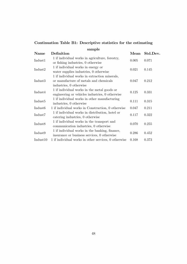
Continuation Table B1: Descriptive statistics for the estimating

sampleName Definition Mean Std.Dev.

Indust11 if individual works in agriculture, forestry,or fishing industries, 0 otherwise

0.005 0.071

Indust21 if individual works in energy orwater supplies industries, 0 otherwise

0.021 0.145

Indust31 if individual works in extraction minerals,or manufacture of metals and chemicalsindustries, 0 otherwise

0.047 0.212

Indust41 if individual works in the metal goods orengineering or vehicles industries, 0 otherwise

0.125 0.331

Indust51 if individual works in other manufacturingindustries, 0 otherwise

0.111 0.315

Indust6 1 if individual works in Construction, 0 otherwise 0.047 0.211

Indust71 if individual works in distribution, hotel orcatering industries, 0 otherwise

0.117 0.322

Indust81 if individual works in the transport andcommunication industries, 0 otherwise

0.070 0.255

Indust91 if individual works in the banking, finance,insurance or business services, 0 otherwise

0.286 0.452

Indust10 1 if individual works in other services, 0 otherwise 0.168 0.373

48

FIGURES

w

a

A

45º

Possible positions of the public package P

UL*

αL*

αΗ*

0

H0

w-ℓ0

0)( =⋅Π L

0)( =⋅Π H

w0Lpw −0Hp−

0Lpw −

0Hpw −

UH*

Figure 1. The competitive equilibrium in the absence of a public health system under symmetric information is (αL

*, αH*).

n

L

0=Π L

U 0( =Π

*Hα

α̂

w-

L

45º a

1

A

Possible positions of the public package P

VIII VI

VII

I II

III

IV

V

)(⋅

L

)⋅H

ˆIX

H0

Figure 2. The competitive equilibrium in the absence of a public health system uadverse selection is ( , αˆLα H

*). The roman numbers label regions used in the proo

w

n

L

U H*

nder fs.