Capt Rick Moore and Capt Steve Johnson, US Air Force, Randolph AFB, TX "A SAS/Graph is Worth a Thousand PROC TABULATES"

You've heard the old cliche--a picture is worth a thousand words. Well, in the world of Air Force personnel analysis, sometimes a SAS graph is worth a thousand PROC TABULATES. Analysts at the Air Force Personnel Center are discovering new and creative ways to bring numbers to life through SAS/Graph software. The focus of this paper is three-fold. First, we'll examine some of the many benefits of using graphs in general and SAS/Graph in particular. Second, we'll discuss two Air Force applications of SAS/Graph. Finally, we'll look at a few of the graphs you can produce with SAS/Graph, and go ''under the hood" to look at the code we used to produce the graphs.

Benefits of Graphs & SAS/Graph

In the Air Force, there has been renewed emphasis in recent years on customer satisfaction. Understanding and then exceeding a customer's expectations is at the heart of the whole Quality Air Force movement. Therefore, let's look at the benefits of graphs and SAS/Graph through the eyes of our customers.

1. "Great numbers, but what do they tell me?" PROC TABULATES and PROC PRINTS are powerful tools to crunch numbers and produce tables of data. Unfortunately, most managers have neither the time nor talent to peruse volumes of data in search of insight. They rely on their analysts to gather the data, and then present it in a way which is easy to read and understand. In most cases, a graph will do a better job of that than just a series of numbers on a page. Graphs allow the customer to quickly assess trends and relationships between data in a format that is pleasing to the eye. While some managers are happy with and may even prefer just numbers, we've found that most managers prefer some sort of graphical depiction of the data.

2. "Great graph, but it's two weeks late!" The real beauty ofSAS/Graph is being able to turn raw numbers into graphs at the push of a button. If you have enough hours in your work day to "fat-finger" data into a large graphics presentation, then you may not need SAS/Graph. But when you have multiple customers who need multiple graphs, and they need them in a couple of hours, a working knowledge of SAS/Graph will sure come in handy. The graphs may not have all the bells and whistles of more advanced graphics programs, but you can turn them around quickly in order to meet a deadline.

3. "Interesting analysis, but it doesn't address the real issue!" Another benefit of using graphs is that they help you focus your analysis in the right direction. There's nothing quite like a pie chart to help you rule out (or rule in) possible causes of the problem you're studying. A quick SAS/Graph can save you hours of time you would otherwise spend scouring through page after page of numbers, in search of a glimmer of insight. Oftentimes a customer will change the focus of our analysis, after seeing some preliminary results on a quick SAS/Graph. That step can make the difference between success and failure, because great analysis is of no use if it doesn't address the real question.

173

These are just a few of the reasons you should consider adding SAS/Graph to your arsenal of analytical tools.

Air Force Applications of SAS/Graph

At the Air Force Personnel Center's Analysis Branch, we've developed some interesting SAS/Graph applications. Two that we'll address here are Career Field Analyses and Enlisted Retention. For each topic, we'll provide a brief background to the project and a sample of the SAS graphs that we produced.

Career Field Analyses. There are nearly 400,000 active duty military members in the Air Force today. Every aspect of their careers, from coming on active duty until separation or retirement, is managed by hundreds of people at the Air Force Personnel Center, located at Randolph AFB, Texas. A wide variety of information is maintained on these individuals in the Personnel Data System, the primary database we use. In fact, we estimate that a total of over 540 million cells of information are maintained on these individuals--everything from gender to duty title to the date they had their last performance report.

As Air Force analysts, our job is to slice and dice all that data in order to answer a myriad of questions that come our way. It may be a simple question, like "How many women pilots are in the Air Force?" or "What percentage of the enlisted force are married?" At other times, the questions are a bit more complex: "How has retention been for the enlisted force over the past ten years, and in particular, for those who. are frequently deployed?" In addition to these types of data requests, we also are frequently asked to perform a full-blown career field analysis for a particular Air Force specialty, i.e., security police or intelligence. The assignment officers or functional managers who manage those career fields want us to measure the health of their career field in a number of different areas. For example, "How is our overall manning situation, and how does our company grade Gunior officer) manning look in comparison to our field grade (senior officer) manning?" Or, "How is our inventory distributed across years of service"? Or perhaps, "Where are the positions for this career field located?"

Prior to discovering SAS/Graph, our approach to these career field studies was effective, but very time-consuming. We began by running numerous SAS programs to generate dozens of tables of data. We then "fat-fingered" the data into a large graphical presentation with lots of bells and whistles. Customers praised the finished product, but unfortunately it took a long time to prepare these masterpieces. Thus, we were limited in how many studies we could accomplish in a particular year.

Then along came SAS/Graph! With SAS/Graph, we are able to convert the career field data (contained in our SAS data sets) directly into graphs. No more sorting through tables of data. No more fat-fingering. With just the push of a button, we can turn volumes of data into a wide variety of very presentable SAS/Graphs. A small sample of the kinds of graphs we produce is shown below.

174

Career Field Graphs - DAFSC 36PX AUGUST .. &WA, LT -LT COL

r-----~----~------------~ r----~------------------~ Permanent Party Manning Permanent Party MannIng AfIC • .,. .urac-JP

AuthorIzatIons By MAJCOM _ ...

-"""-- _ ... -....

We are able to generate these graphs for any career field we desire, simply by targeting that career in a macro statement. Bottom line: we can generate a wide selection of graphs on numerous career fields in a matter of hours. That sort of production would have taken weeks, even months, using our old approach. Due to this increase in efficiency, we've been able to generate a set of the most popular graphs to every assignment officer--for evexy career field--in iust 2 days!! Feedback from these customers has been very positive--they like the way the graphs look, and they really appreciate the quick turnaround time. And as we mentioned above, the graphs allow them to quickly locate problem areas that need attention.

Retention of Enlisted Force. In addition to career field studies, our retention analysis has benefited from SAS/Graph. Enlisted members of the Air Force reach points in their careers where they must make the decision to continue their Air Force careers - to "reenlist" - or to separate from the service. If members elect to continue their careers, then we might conclude they have a positive perception of their type of work, future opportunities, and overall quality of life. For obvious reasons, Air Force leadership is always interested in the percent of eligible members who decide to continue their careers. This gives them an indication or pointer as to the "health" of their company. The term used to convey this "health" is the "reenlistment rate".

175

Reenlistment rates and their trends over time are closely monitored by Air Force leadership, as evidenced by their monthly requests for reenlistment analysis. However, our leaders at the Pentagon aren't the only ones interested in retention. We receive requests for reenlistment statistics from career field managers, service managers, graduate students, civilian organizations, and other base agencies and personnel. So you can see the demand is quite great and, of course, everyone who asks for numbers wants them deciphered as well, hence the need for a picture.

/ REENLISTMENT RATES BY MARITAL STATUS/ AS31_M

First Tenn Ainnen .. .,----------------,

" · : u

~ · " ~ -e-----...... ____ -.4----.-.... -: --l .. --rtr'"--------..

~---------

:

"~ ".-

....... --.~-~.--u~-~.--"~-~_ "'''--

Career Ainnen ... .,----------------,

~ I~

~ .. u I , · · .. , ·

....... --.--::-.-~.~-::-.--.,.-------'-

. , ~ i . : ,

Second Tenn Ainnen .. .,----------------,

.. -<,..--.~-~.--.~-~.--.~-...,J_ 1 ..... _ eoe-e..- I

Career Ainnen Over 20 YOS .. ...

..

..

..

..

.. . 1 ... 09_ Ges.... I

We're not sure whether it was necessity (the mother of invention) or our own laziness which drove our current applications of SAS/Graph. Prior to making use of SAS/Graph, we created many tables of multiple crossings of reenlistment rates. This was "cool stuff" for the analyst­more numbers to describe the world. Of course, the boss usually wants us to reduce all these numbers to a simple conclusion without all the "geekspeak". Alas, we used supercharged, "bells and whistle" -packed, resource-hogging programs to reduce these numbers to simple graphs. Great, no more stories to write! Unfortunately, the time saved by not writing up the detailed conclusion was quickly consumed, and then some, transferring data from a SAS table to a graphics program - a giant time sink! So, we had to ask ourselves, "Do the benefits of the 'bells and whistles' of some graphics program outweigh the time lost and little value added?" Our

176

answer was no! So we turned to SAS/Graph. Now with the use of SAS/Graph and a few keystrokes, we generate multiple graphs (see above) telling the reenlistment story - an upward line brings smiles to all, a downward line leads to more questions (and overtime) for the analyst. With a simple change in the graphics options, the graph is neatly wrapped up into a finished product, format ready for multiple software packages to include Microsoft Word, Corel WordPerfect, or for transfernng to the World Wide Web (graphics interface file (GIF» to be shown to the world!

However, innovation is sometimes our own worst enemy. After showing off our SAS/Graph battle scars and our great graphs to others, we were presented with that ultimate challenge: "Cool graph, but what else can it [you] do?" So began our fun SAS/Graph adventure.

SAS/Graph Capabilities-A Primer

We'll now take a closer look at just a few of the many different graphs that can be produced with SAS/Graph. This is not intended to be a tutorial, but rather an attempt to share a few of our SAS/Graph experiences, applications, and survival tricks we've learned along the way. These graphs were produced on SAS 6.11 running under Windows 3.J on a Pentium J 00 MHz system.

Bar Charts

Example 1:

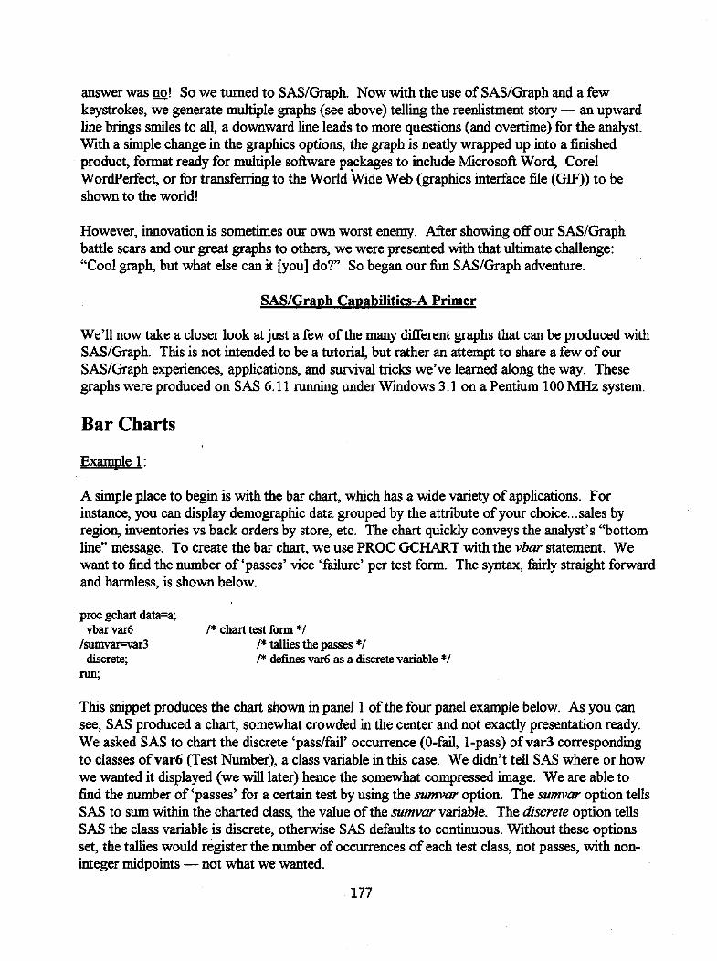
A simple place to begin is with the bar chart, which has a wide variety of applications. For instance, you can display demographic data grouped by the attribute of your choice ... sales by region, inventories vs back orders by store, etc. The chart quickly conveys the analyst's ''bottom line" message. To create the bar chart, we use PROC GCHART with the vbar statement. We want to find the number of 'passes' vice 'failure' per test form. The syntax, fairly straight forward and harmless, is shown below.

proc gchart data=a; vbarvar6

Isumvar=var3 discrete;

run;

1* chart test form *1 1* tallies the passes *1 1* defines var6 as a discrete variable *1

This snippet produces the chart shown in panel I of the four panel example below. As you can see, SAS produced a chart, somewhat crowded in the center and not exactly presentation ready. We asked SAS to chart the discrete 'pass/fail' occurrence (O-fail, I-pass) ofvar3 corresponding to classes ofvar6 (Test Number), a class variable in this case. We didn't tell SAS where or how we wanted it displayed (we will later) hence the somewhat compressed image. We are able to find the number of 'passes' for a certain test by using the sumvar option. The sumvar option tells SAS to sum within the charted class, the value of the sumvar variable. The discrete option tells SAS the class variable is discrete, otherwise SAS defaults to continuous. Without these options set, the tallies would register the number of occurrences of each test class, not passes, with non­integer midpoints - not what we wanted.

177

- __ -!lor _-.... -

a 3 • -___ -IIor-__ JIIIlIPaIInI1Dr _,.,. "..,....,.. __ !lor __ _

~,------------------------,

1 2 • 4 1 2 • 4 1 a I 4 ... ......

I--- ... ---I I-- • --! I-- II ---1 ..... .....

In ~, _II _. Example 2:

2 a .......... ____ IIor_ ...... ---....

• --.. =F _II _.

4

Moving on to panel 2, we see our labels are in clear text, our horizontal scale (midpoint axis) is scaled to the panel, and our vertical bars are wider and topped with tallies. The syntax below shows options and definitions that were added to enhance the chart.

*** Add Axis and Bar attributes;

1* Define symbol and axis characteristic *1

** length - percent of graphics window; ** label - Clear text for axes;

axis! length=80 label = (,Test Fonn'); *** Midpoint Axis; axis2 length=65 label = (Nwnber Passed'); *** Response Axis;

proc gchart data=a;

178

vbarvar6 Iframe discrete sumvar=var3 type=sum sum raxis = axis2 maxis = axisl width=22 space = 3;

run;

1* produces a frame around the graph *1

1* defines type of statistic to calculate *1 1* labels the vertical bar with the sum statistic *1 1* use axis2 definition for response axis *1 1* use axisl definition for mid-point axis */ 1* defines width of bar */ 1* defines space between bars */

The comments included in the snippet above describe the purposes these additional options serve. Our raxis (response axis) and maxis (midpoint axis) are defined by axis definitions outside of the vbar options. The axisn options offer the user a wide range of control over axis presentation to include, "select and order major tick marks, change the number and appearance of major tick marks, change the text of the axis label and tick marks, modifying the appearance of the axis, including length, line, line style, and position"(I). The axis length option used above defines the portion of the graphics window the axis will cover. In this case, we've defined the first axis to be 80 percent of the window. The second axis length has been defined as 65 percent. The unit of measure is percent since we defined this as the default graphics unit of measure in our goplions statement.

This is probably a good time to talk about the graphics options. The ones used to produce these charts are shown below.

goptions reset=g1obal gunit=pct border rotate=landscape fiext=swissb htext=3 device=win;

SAS/GRAPH technical manuals provide a complete discussion of graph options. We'll touch upon a few of them here. From the "SAS/GRAPH Software Usage Version 6", first edition:

resel=global: "resets all global statements, all global statements except the goptions statement or individual global statements, respectively."

Gunit=pct: "selects the default units for options that use IN, CM, PCT, or CELLS as the units. The GUNIT= option does not affect options that use only IN or CM as the units."

border: "includes a border around the graphics output area."

rotate=landscape: "Causes the graph to be rotated 90 degrees on the device. ROTATE can only be specified with certain hardcopy devices."

jtext=swissb: "selects the default font for all test in the output".

htext=3: "selects the default height of all text in the output." Related to the htext option but not used in the above gop/ions statement is the htitle option. This option selects the default height of the first title line, overriding the htext settings.

179

device=win Specifies the graphics output device driver. In this case the Windows default driver is used. However, SAS provides a very large list of optional drivers. A list of device drivers for such applications as Microsoft Word or Corel WordPerfect, or for transferring to the World Wide Web (graphics interface file (GIF» can be found in the SASHELP library, DEVICE catalog. Another related device topic not shown in the example goptions statement is the targetdevice option. This option displays the output as it will appear on another device.

Once you have the graphic presentation-ready, you may want to export it to your presentation application. The following goptions statement is an example of how this is done.

filename gph_out 'c:\sasdata\sugichrt.cgm'; goptions gunit=pct border rotate=landscape fiext=swissb htext=3 device=cgmmwwc gsfname=gph_out gsfmode=repJace;

The device in this case is the color computer graphics metafile (CGM) driver for Microsoft Word for Wmdows. The graphics stream file (GSF) name points to the filename handle "gph_out" defined by filename. When a new file is created, replace option allows the old file to be overwritten.

Example 3:

In our third chart, we show the use of groupings, gray shading (color is also an option) and introduce a statistics option. The code below was used to produced the chart in this example.

1* use either color or gray scale (hex) *1 1* patternl value=solid color=yellow; *** define bar patterns and colors; pattern2 value=solid color=blue; *1 patternl value=solid color=gray30; *** define bar patterns and colors; pattern2 value=solid color=grayaf;

axisllength=70 label = fTest Form') ; *** Horizontal Axis; axis2length=60 label = ('Pass' justify--center 'Proportion'); *** Vertical Axis;

** * add group axis definition; axis3 label = ('Test Year); *** Group Axis, length not supported with groups;

proc gchart data=a; vbarvar6 Iframe discrete sumvar=var3 type = mean Taxis = axis2 maxis = axisl gaxis = axis3 group=varl

1* use axis3 definition for group axis definition *1 1* group defined as varl "'I

180

subgroup = varS pattemid = subgroup mean coutline=black width = S space=2;

label varS='Sex'; ron;

1* subgroup defined as varS *1 1* apply pattern definition to subgroups *1 1* label bars with mean value *1 /* outline bars with black borders *1

*** clear text varS;

In this example, we've taken more control over the bar appearance with the use of the pattern statement. In these pattern statements, we've set the color or gray scale to solid vice various densities of SAS default crosshatch or diagonal patterns. The color may also be set here as well by using color keywords.

Also in this example, we've grouped our data presentation into years and further subgrouped into sex categories. Since we've created groups, a third axis has been included to control the appearance of the group axis. There is no axis for the subgroup since they reside within the group and are identified as different levels of gray within the bar.

The last addition to this chart is the "mean" statistic. We select the mean statistic with the type option. Available statistics include frequency, percent, cumulative frequency, cumulative percent, sum and of course the mean. When requesting the sum or mean statistic, the sumvar option must be used also.

Example 4:

The final vbar example shown in panel 4 is the block chart. The block chart presents the data in a three dimensional form using the row and columns to designate groups - very much like a graphical PROC TABULATE.

We produced the block chart using the same code used in the vbar example above and changing vbar to block -- that's all.

This discussion ofPROC GCHART barely touched upon the subject. The SAS documentation is very extensive and illustrative. In addition, SAS 6.11 provides a bundle of examples illustrating the vastness of options and their effects. You say, "Cool graphs, but what else can SAS do?" So, let's look at other ways the data can be presented. For example, your boss may like to see lines instead of bars, so let's take a look at some SAS/Graph plot options.

Plot Graphs

Plot Example 1:

Familiar to the analyst is the scatter plot, a common use ofPROC GPLOT. But, creating a two variable scatter plot is only a fraction of the capability ofPROC GPLOT. Our applications of

181

gpiot include enlisted retention trends, plotting shapes of distributions, comparing hiIlows, comparing one demographic characteristic effects relative to another characteristic on a dependent variable, and much more. Our GPLOT illustration begins with the scatter plot. The syntax, shown below, like that of GCHART, is again simple and straight forward.

proc gplot data=a; plot score*age

/frame; run;

This code produced the graphic shown in panel 5 below.

-100

10

10

7D

.,

--.. 71

10

II

_ SAIioQIph __ '" 1101>_

21 12 IS

AIlE -. 1-15AIiI\InIph.....-..... - --I

21

~ ~

25 21

_ SAt/IlnIpII1IoD __ PIoI _____ --.. 10

.' ......... .... ~.

'. f .~ IV 1···· .. ·· .. / 71

IV

2D

I- -- F MI

ZI 12 IS II 21 -_. 1_ UII/GIIIpb 1101>-_ - ..... 1

t - __ aD

* .. ...,.. 21

• IV M IV • II • • --

lIS

Using SAS defaults, a well formatted scatter plot is produced. We can immediately see there does not appear to be any significant outliers, some clustering around the score of 80 and a slight upward trend for the older students. Now, after seeing the scatter plot patterns, we want to condense our data down into descriptive statistics and see the underlying trends.

182

Plot Example 2:

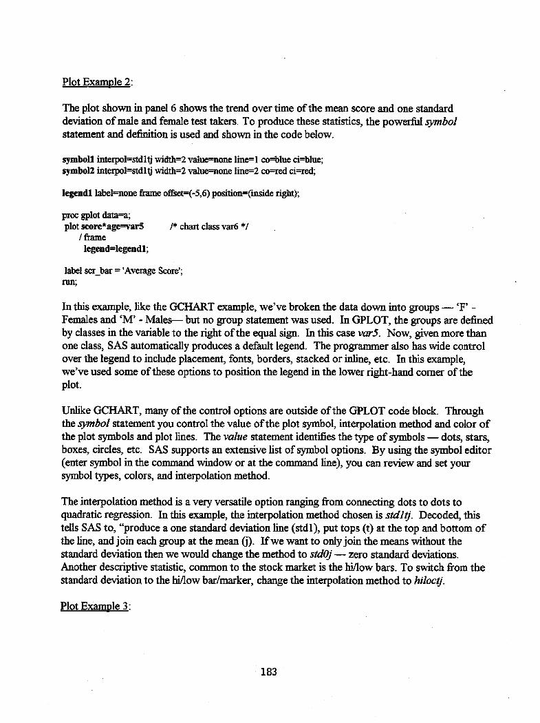
The plot shown in panel 6 shows the trend over time of the mean score and one standard deviation of male and female test takers. To produce these statistics, the powerful symbol statement and definition is used and shown in the code below.

symboll interpol=stdl1j width=2 value=none line=l co=blue ci=blue; symbol2 interpOl=stdl1j width=2 value=none 1ine=2 co--re<l ci=red;

legendllabel=none frame offset=(-5,6) position=(inside right);

proc gplot data=a; plot srore*age=varS

1 frame legend=legendl;

1* chart class var6 *1

label seT_bar = 'Average Score'; run;

In this example, like the GCHART example, we've broken the data down into groups - 'F' -Females and 'M' - Males- but no group statement was used. In GPLOT, the groups are defined by classes in the variable to the right of the equal sign. In this case var5. Now, given more than one class, SAS automatically produces a default legend. The programmer also has wide control over the legend to include placement, fonts, borders, stacked or inline, etc. In this example, we've used some of these options to position the legend in the lower right-hand comer of the plot.

Unlike GCHART, many of the control options are outside of the GPLOT code block. Through the symbol statement you control the value of the plot symbol, interpolation method and color of the plot symbols and plot lines. The value statement identifies the type of symbols - dots, stars, boxes, circles, etc. SAS supports an extensive list of symbol options. By using the symbol editor (enter symbol in the command window or at the command line), you can review and set your symbol types, colors, and interpolation method.

The interpolation method is a very versatile option ranging from connecting dots to dots to quadratic regression. In this example, the interpolation method chosen is stdltj. Decoded, this tells SAS to, "produce a one standard deviation line (stdl), put tops (t) at the top and bottom of the line, and join each group at the mean (j). Ifwe want to only join the means without the standard deviation then we would change the method to stdOj - zero standard deviations. Another descriptive statistic, common to the stock market is the billow bars. To switch from the standard deviation to the billow bar/marker, change the interpolation method to hi/octj.

Plot Example 3:

183

As we mentioned before, the interpolation method also includes options for regression. In this example, panel 7, we again changed only the interpolation method to interpol=rqclm90 for the first symbol (the 'F' group) and interpol=rq for the 'M' group.

symboll interpol=rqclm90 width=2 value=circle height=2 cv=blue co=black; symbo12 interpol=rq width=2 value=square height=2 cv=red;

legendllabel=none frame offset=(-5,6) position=(inside right) across=l;

Again, allow us to decipher. For symboll, we've asked for a quadratic regression with a plot of the confidence intervals at the 90 percent confidence level around the mean. In symbol2, we've only asked for the quadratic regression. The parameters for the model are displayed in the SASLOG and at the time of this writing, we hadn't found how to get these parameters to a~tomatically show on the plot. You may also notice that the symbols have returned. Using the value option we've assign circle symbols to the female group and square symbols to males.

Plot Example 4:

Often the analyst is faced with a three parameter relationship and may need to show the parameters' multiple interaction. A surface or contour plot may ''water the eyes" of those fluent in "geek-speak" but often cause the eyes of management to glaze over. So, we choose to substitute a two-dimensional looking chart with three parameters (which can also be further broken down into classifications as well). Our final panel, panel 8, illustrates the interaction of three parameters using two vertical axes. The following code was used to generate the plot.

axisllabel=('Funding') order=(20 to 32 by 2); axis2 label=('Test Year'); axis3label=('Test' justify--center 'Score');

symboll interpol=join font=marker value=Q height=5 co=blue; symbo12 interpol=join font=marker value=V height=5 co=red;

proc gplot data=b; plot score*year

I frame haxis=axis2 vaxis=axis3; legend=legendl;

pl0t2 budget*year I frame

haxis=axis2 vaxis=axisl;

run· ,

1* chart class var6 *1

Probably the most noticeable difference between this snippet and the previous code shown is the use of plot and plot2. Notice also that they both share the independent variable 'year'. Plol2 generates the right-hand vertical axis. Since we have an additional axis, we've defined a third axis

184

statement. You may recall from above, SAS automatically generates a legend when you have more than one class in a field. In this example, we have not defined a group variable and hence no automatic SAS-generated legend. SAS uses special marker symbols to clearly identify the line (symbolically) and to which axis it belongs. This may not always be an option for you and your application. Using the note command, you can build your own legend. The code below was used to generate the legend shown in panel 8.

note move=(68,68) color-blue font=marker 'Q' f~mt=swissb ' - Test Scores' move=(68,-5) color=red font=marker 'V' font=swissb' - Budget';

We've told SAS/GRAPH to move to position right 68 percent and up 68 percent and insert marker font 'Q' (Male silhouette), then using font Swiss Light insert' - Test Scores'. We reposition, move down 5 percent and insert our legend text for the budget.

Again, we've only touched upon a small portion ofGPLOT's capabilities. We encourage the reader to experiment and test the capabilities of GPLOT. The examples we have shown have been part of a single graphic composed of multiple panels. We will now move on to discuss how to create these multi-panel displays with PROe REPLAY.

PROCREPLAY

We believe the best way to think about PROe REPLAY is in the terms ofa merge. For, example, four charts were merged into one graphic using a template that defined the graphics window into four panels with white space between them. Now let's take a look at the code that merged these files into one graphic.

proc greplay igout=gseg tc=sashelp.templt template=12r2s nofs; treplay l:plotl 2:plot3 3:pl0t2 4:plot4; quit; *** ends greplay;

Starting from the top, we enter PROe GREPLAY and tell SAS/GRAPH where to locate the graphs to merge. In this case, they are located in the work.gseg default catalog, a graphics work area created by SAS. Next, we identify to SAS the location of our four-panel template named l2r2s. Our template is located in the template catalog tempit pointed to by the libre! sashelp. The template name identifies the panel definition type. For example, left 2 right 2 panels with space between. If you open the template catalog you'll see all the SAS-provided panel templates. The final command is no/s, which specifies GREPLAY should use line mode. In line mode, you can use the GREPLA Y line-mode statements: FS, LIST, PREVIEW, REPLAY, and TREPLA Y. Otherwise, GREPLAY, when executed would open the GREPLAY window.

On the next line we use the command treplay to identify to SAS which graphics to use and which panel to insert them into. In this case we've identified plots 1-4 to insert in panels 1-4. Where did plots 1-4 come from? For lack of confusion, we did not show in the previous chart and plot snippets the uses of the name option. The example code below generates our first chart example with the name of 'plot l' included.

185

proc gchart data=a; vbar var6 1+ chart test form +1

Isumvar=var3 1+ tallies the passes */ discrete name='plotl'; 1* defines var6 as a discrete variable */

run;

After running this code, look in the work.gseg catalog; there you will find the catalog entry 'plotJ'. For each chart and plot generated in our example, we assigned a unique name.

If you're using PC SAS and make several runs while adjusting your final product, you need to clear out the previous graphs. Otherwise, SAS renames these graphs and GREPLA Y won't find them. The following code will clear the old graphs out before you regenerate new graphs.

proc greplay igout=gseg tc=sashelp.templt template=12r2s nofs; deletel:plotl 2:plot3 3:plot2 4:plot4 template; quit; *** ends greplay;

Now, what do you do when SAS does not have the template you need? You create it!. To do this you need to enter the template design window. Use the following code substituting your Iibref and catalog names to access the window.

Syntax.: proc greplay igout=librefcatalog tc=librefcatalog template="new _template_name"; run;

Example: proc greplay igout=sasdat.mytemp tc=sasdat.mytemp template=head2p; run;

After submitting the code, you'll be at the GREPLAY window. At the command line enter "Edit your _new.Jemplate _ name.template". This will bring you into the template design window. Now you can start experimenting and designing your own panel.

A few final notes on PROC GREPLAY. Returning to our first two examples, you may notice a header/title that spans the entire graphics image. SAS does not provide a template such as this, so we built a new one, a five panel slide. While building this panel, we discovered a couple properties of the template. First, all the graphic sources do not have to be the same. You can mix and match charts, plots, slides, etc. Second, the panels may overlap each other. Using this overlapping property is how we develop the format for the graphics shown earlier. In the case of the GSLIDE product, the space allocated to that graphic needs to cover 100010 of the graphics window. Why so? If you only assigned the GSLIDE to the top, say 20 percent, then your title would be very small, about 4 percent of the graphics window. Now assuming you use the GSLIDE for the title only, and you've placed the title at the top 10 to 20 percent, you must leave about the top 20 percent of the graphics area uncovered by your lower panels. Now organize your lower panels into the preferred groupings.

186

So what happens when you merge these all together. First, GREPLA Y finds the GSLIDE graphic and places in its assigned panel. Next, GREPLA Y finds the remaining graphics and writes them into their assigned panels while masking the lower 80 percent (hopefully blank) GSLIDE image. The finished product is a multi-panel graphic with a nice clear banner at the top.

The GREPLA Y facility allows your creativity to go unconstrained. We failed to mention that you can replay many plots on to the same panel if you have the need to overlay a plot on a bar chart. Knowing you can overlay many on one or one into many or many into many gives you much latitude in creating the graphic that makes the point!

Summary

We discussed a few of the many benefits of using graphs and SAS/Graph. We showed a couple of Air Force applications of SAS/Graph. We then introduced several SAS/Graph capabilities, including different procedures, templates, and options. However, we were only able to scratch the surface. Other interesting SAS/Graph capabilities include horizontal, pie and star charts, and 3-D scatter, surface, and contour plots. You should also explore the annotate facility, and all the fun things you can do with data and maps. We believe the graphic is a clear and precise way to tell the story, to get to the "bottom line" quickly. SAS/Graph is definitely a tool you should check out.

Reference

SAS Institute Inc. (1991), SAS/GRAPH Software: Usage Version 6, Cary, NC: SAS Institute Inc.

187