Capital Markets: Monetary and Fiscal Policy … Markets: Monetary and Fiscal Policy Determinants ......

Anderson 1

Capital Markets: Monetary and Fiscal Policy Determinants

By John Anderson

Creighton University

Investment 101

Capital markets are central to a country’s market economy. The United States

and other industrialized countries have played a vital role in establishing these

international markets. Capital (stock) markets represent the economic strength and

development of a country. Countries with strong capital markets have a high level of

economic development because there is a greater propensity for investment. Investment

leads to technological innovations and greater economic development. Over the past

fifty years, investors have taken an active role within both their own and foreign

countries vis-à-vis the capital market. Investment, however, has not been uniform across

the world. While some countries have robust capital markets, others seem to be lagging

behind.

The United States has one of the strongest capital markets in the world with

strong investment patterns from both domestic and foreign entrepreneurs. After the

worldwide recession, American markets seem to have rebounded and stabilized. France,

however, has not had same good fortune as the United States. The capital market of

France is relatively weak even compared to other neighboring European countries and

most certainly does not compare with the United States’ capital market. Yet, France’s

capital market is strong compared to that of Chile’s capital market. How do we explain

the varying degrees of strength in capital markets cross-nationally?

Anderson 2

Investment that is provided by the banking industry through debt, equity and

savings allow entrepreneurs to invest their capital into the markets. These investments

spur economic growth and provide opportunities for other investors to enter the market.

There are six different ways to define market strength, gross domestic savings, private

domestic credit issued by financial intermediaries, foreign direct investment, the amount

of liquid liabilities, market capitalization and the amount of market turnover. The

strength of capital markets is invariably dependent upon investors who purchase stocks

on credit from financial intermediaries. These loans allow the investor to explore other

possibilities with their own personal finances. Investors looking for the best payoffs will

look for a country with low corporate taxes, interest and inflation rates, as well as strong

exchange rates.

Although research has been extensive in scope, there is still no definitive answer

as to what makes for a more robust capital market. The literature tends to focus on three

specific theories: law and finance, endowment and finance, and politics and finance.

Each theory posits different ideas and reaches different conclusions concerning the

strength of capital markets. In recent years, scholars have found empirical evidence to

support the association of legal origin and legal protection to capital markets; however,

the wealth of research on these subjects does not take into account the full body of causal

relationships. For the most part, studies have focused explicitly on three theories, law

and finance, politics and finance, or endowment and finance and their association with

strong capital markets. An exception is that of Beck, Demirguc-Kunt and Levine (2001)

who examine the three theories in competition with each other.

Anderson 3

I propose to examine the Law and Finance, Politics and Finance, and Endowment

and Finance theories in competition with a monetary & fiscal policy hypothesis. I

hypothesize that lower taxes, inflation and interest rates as well as strong exchange rates

lead to stronger financial markets and consequently, stronger capital markets. The

monetary & fiscal policy of the government determines the value for these rates, and with

such control, has the power to strengthen the capital market. These concepts should

determine the relative level of investment within the capital market and the amount of

economic growth.

This work will examine the affects of monetary & fiscal policy on capital

markets. The theory will be tested holding the political, geographical, and legal systems

constant. This empirical approach will either validate previous findings in the literature

or provide new directions for the study of capital markets by economists or International

Political Economy (IPE) scholars. It is hoped that this research will also help those in

business and the academic communities to understand the inter-workings of politics,

policy, law, and environment on capital growth. In addition, this research is intended to

provide investors with indicators, which if used properly, could explain the robustness of

markets worldwide. Essentially, these indicators will help investors decide in which

market, if any, they should invest.

The research will compare 47 countries (those used by La Porta, Lopez-de-

Silanes, Shleifer and Vishny (LLSV) (1997, 1998)), focusing on the year 1999, for which

the information is most readily available. The timeline for the data in this study varies

due to incomplete information and the restrictive information policies of some countries.

The countries included are a good representation of countries with stable political and

Anderson 4

market systems. Even though each country has a different political and legal structure, as

well as unique geographical areas, these countries should provide for an acceptable

sample to test the dependent and independent variables.

Four Schools of Thought:

There is a substantial amount of literature on the topic of financial markets and

economic growth. The seminal works of Adam Smith (1776, 1911), John Maynard

Keynes (1936) and Modigliani & Miller (1958), and Goldsmith (1969) describe the

fundamental dynamics of financial development within the economic sphere. Their work

provides the theoretical foundation for the development of alternative theories concerning

the question of capital markets. These theories can be divided into four schools of

thought related to the development of capital markets: politics and finance, monetary &

fiscal policy and finance, law and finance, and endowment and finance.

The politics and finance theory, grounded in the work of North (1990), posits that

political, social and economic institutions shape the long-run performance of the

economy (North, 107). These institutions change over time, and the impact of that

change has more of an effect on economic and financial development than any one single

determinant. This fact led Stephen Haber (1991) to research the history of political

institutions and examine their effectiveness in financial and capital market development

within the United States, Brazil and Mexico. Haber (1991) found that the political

institutions of these countries had different policies toward financial investment,

especially early in their histories. Brazil, after the removal of their monarchical system,

created more lax restrictions on the financial market. This along with better legal rules

for investment led to the growth of the banking industry and the capital market. The

Anderson 5

better rules and easier access for entrepreneurs to capital markets loosened the control of

the wealthy elite in Brazil, creating an open market for investment.

This however was not the case for the people of Mexico. The wealthy elite of

Mexico ruled with an iron fist and were able to create legal and political barriers to entry

in the banking industry. The entire financial system became the political machine for the

ruling class. In many cases, the ruling class made it impossible for an entrepreneur to sell

equity in an investment without receiving some compensation for the transaction. The

ruling elite, as rational actors, wanted to limit outside investment to protect their assets

and maximize their profits without any undue competition.

This rational choice theory was developed from an older theory associated with

hegemonic powers. Mancur Olson (1993) argues that the actions of those in power,

especially in monarchical and authoritarian governments, have a direct correlation with

what is widely known as the hegemonic stability theory. The leaders control the means

of production, as well as the financial sector. This control produces stability within the

country. However, absolute power and control will eventually lead to corruption and a

decline in economic growth. This hegemonic stability theory supplemented by the

rational choice model led Haber (1991) to hypothesize that the capital markets of

developing countries, such as Mexico, have less market capitalization because of the

political constraints placed on financial intermediaries. These constraints led to poorly

defined property rights and government regulatory policies. The high level of autocracy

that exists within the political institutions leads to a greater concentration of industry in

fewer peoples’ hands, which slows capital growth and contracts capital markets.

Anderson 6

The monetary & fiscal policy and finance theory is an extension of the politics

and finance theory. The seminal works of Adam Smith (1776) and John Keynes (1936),

supplemented by Goldsmith (1969) and McKinnon (1973) provide the foundation for the

theory, which argues that sound monetary and fiscal policy helps to develop strong

capital markets. Goldsmith (1969) in his study on economic development determined

that the only financial variable, which had any impact on economic and capital growth,

was strong inflation (Goldsmith, 48).

Meek (1960), in an earlier article, examined these economic impacts by looking at

the role that federal deficits play in regards to capital market strength. The classical

economic theory states that deficits cause interest rates to rise and these interest rates

‘crowd out’ investments slowing economic growth. Meek (1960) contends that the

United States should revive its international capital markets because external investment

is necessary to lower the cash deficit. Meek (1960) hypothesized that to encourage the

growth of capital markets one should increase the availability of alternative sources of

finance; reducing tariffs in order to make the market more competitive; and pursue anti-

inflationary monetary policies. These policies working in unison create an openly

competitive market that welcomes entrepreneurs to invest in capital markets without fear

of losing their investment because of unsound government policies. The government

fiscal policies have an effect on capital markets. Corporate taxes and tax policies are an

example of how the government attempts to control investment, and indirectly the

strength of capital markets.

Adam Smith (1776, 1911) laid the groundwork of tax policy, which would then

eventually be empirically tested by Ross Levine (1991). Smith (1776, 1911) had argued

Anderson 7

that higher taxes would lead those with capital stock, who were not tied to a specific

country, to invest in countries with lower rates because they could make more profit.

Levine (1991), extending the theory, argued that certain tax policies change investment

incentives for entrepreneurs. Many countries have capital gains taxes, which are taxes

taken out of retrieved investments. The rates vary from country to country, and the tax is

very effective. In many cases, the tax policies act as a barrier to entry for the would-be

investor. Entrepreneurs who invest in capital markets are placing their capital at

considerable risk, and to see most of their returns taken away by taxes stifles the capitalist

spirit. However, certain tax policies can stimulate economic growth by creating

incentives for entrepreneurs to invest within the capital markets. Levine (1991)

hypothesized that a tax policy of increasing consumption with a reduction in corporate

taxes would stimulate long-term economic and capital growth.

The law and finance theory similar to the monetary & fiscal policy theory is an

extension of the politics and finance theory. Law is the practical application of politics in

society and the development of its control within the financial system demand a separate

field of study from the politics and finance theory. The financial system is dependent

upon the government vis-à-vis the legislature to create laws, which regulate the financial

industry and determine economic growth. The amount of research on this topic is

extensive, and most of the empirical data is derived from studies conducted by La Porta,

Lopez-de-Silanes, Shleifer and Vishny, hereafter referred to as LLSV. The work of

LLSV (1997, 1998) focuses on the legal determinants of financial development. They

argue convincingly that though there are financial aspects to determining economic and

capital market growth, the best predictor is associated with the country’s legal system.

Anderson 8

The legal system provides investors with rights necessary to conduct financial

business with the state. There are two types of legal systems; one is based on common

law and the other civil law. Common law is law developed through judicial precedent

and enacted through statute by the legislature. Common law strengthens the rights of the

citizens compared to the legal rights of the state. This system, developed in England after

the Viking occupations, brought law into the surrounding country.

Civil law is law based on legislative decree. This system, enforced by

magistrates, strengthens the legal basis of the state in comparison to its citizens. This

system is modeled after ancient Roman law and the Napoleonic codes. The German,

French and Scandinavian legal systems fall into this category, as they historically had

more encounters with the Roman Empire. These legal systems were emulated in

colonies, and as a result, one can trace the financial institutional differences of several

countries back to the legal origin of its colonizing country. LLSV (1997, 1998)

hypothesize that the development of different legal systems, especially their origin,

affects the growth and robustness of the financial and economic growth within a country.

The work of Modigliani and Miller (1958) provides the foundation for a

behavioral financial model working within the law and finance theory. Modigliani and

Miller (1958) found that debt has a fixed interest on its payment, while in the equity

market the investor is entitled to dividends. These dividends provide incentives for future

investment because there is more money being brought in by the investor. As is stated in

LLSV (1998), this is not the entire story and they propose that the essential determinant is

investors’ rights. They argue that rights are inherently created by the legal system of the

country. LLSV (1998) hypothesize that the country with the strongest legal protections

Anderson 9

for investors would thus have the strongest financial markets and a stronger more robust

capital market. Investors, knowing a legal apparatus protects their investments, are more

willing to extend their credit and invest in capital markets. The legal protections

provided give the diversified investor more options and ease the entrepreneur who might

want to invest in a specific country.

Montesquieu (1748) laid the foundation for the endowment and finance theory.

In one of his many works, Montesquieu (1748) argued that merchants would examine the

environment (climate and terrain) of a state to determine if trade were possible in that

region. The groundwork developed by Montesquieu led Hausmann (2001) to examine

research and development (R&D) in tropical countries. Hausmann (2001) found that

tropical countries have a lower GDP because the R&D in these countries is considerably

less because there is little western investment. Western investment is sparse because the

cure for a tropical disease is less likely to make money than a possible cure for heart

disease or cancer. For Hausmann (2001), the only way to rectify the geography trap was

greater globalization, especially in the development of international transportation, global

governance and R&D.

The work of Hausmann (2001) and others on the development of institutions,

whether global or domestic, has spawned a new theory, which perhaps better explains the

causal relationship between endowment and economic development. Easterly and Levine

(2002) and Acemoglu, Johnson and Robinson ((2001) henceforth called AJR) have done

extensive research into this topic and have developed an institutional endowment theory.

Endowments have been an important part in developing economic institutions

throughout the colonial and modern times. AJR (2001) theorize that the colonization by

Anderson 10

European powers in the 16th century frequented both rich and poor countries. The

countries today, however, have seen a reversal in fate; the rich countries are now poor

and the poor countries have become wealthier. This is because of what AJR (2001) call

an “institutional reversal”. The poorer countries were developed in a way that invited

economic growth, while the established institutions within the richer countries were left

unmolested. AJR (2001) argue that the organization of society provides a better

explanation for economic growth because of the incentives that the institutions offer to

obtain investments. AJR (2001) suggest that to measure economic growth one must look

at the institutional quality, enduring quality of the institution, and colonization strategy of

the European settlers. The colonization strategy developed by AJR (2001) is a strong

model, however Easterly and Levine (2002) believe that it does not explain everything.

Easterly and Levine (2002) contribute a three-fold model that assesses the policy,

institutional, and environment views. They theorize that the tropics, germs and crops do

not affect economic growth directly; however, they do have a hand in shaping the

institutions that determine economic policy and growth. The shaping of these political,

legal and economic institutions began during colonization. The environment in several

countries forced the establishment of legal and political institutions quicker than in some

countries. It was these institutions that survived post-colonialism and were shaped by

their environmental resources that now determine economic growth of a capital markets

and the country. Easterly and Levine (2002) contend that the institutional theory explains

a great deal about economic development, and their study develops a new twist to the

institutional view discussed in AJR (2001).

Anderson 11

There has been extensive research done on the foregoing theories, but only one

study conducted by Beck, Demirguc-Kunt and Levine (2001) has developed a framework

to test the theories proposed in this literature review. The empirical evidence from this

study provides strong empirical evidence that legal traditions explain a great deal about

the growth of capital markets and financial growth. Beck, Demirguc-Kunt and Levine

(2001) found that the French legal system had the weakest protection of investor and

property rights as well as a significantly lower amount of capital development. Common

law legal systems fared the best with strong property rights and investor protections,

while keeping a strong robust capital market. The empirical evidence finds moderate

support for the endowment theory. Beck, Demirguc-Kunt and Levine (2001) found that

countries that are situated in poor geographic areas with small resource bases tended to

have less developed financial systems. The empirical evidence for the political theory

was the weakest of the three. The value of the political variables did not provide a

significant statistical relationship between political structure and its affects on capital and

financial development. However, Beck, Levine and Demirguc-Kunt (2001) did not

measure the effect that a countries monetary and fiscal policy may have on both domestic

and foreign investors.

I will test all of the foregoing hypotheses in competition with my own monetary

& fiscal policy hypothesis. Each of these hypotheses seems to answer the question of the

strength of capital markets, but I expect to find greater support for my hypothesis. The

reason I have chosen this hypothesis is that the literature of Smith (1776, 1911) and

Keynes (1936) seems to support such justification. The monetary & fiscal policy theory

postulates that interest rates, inflation rates, corporate taxes and exchange rate policy

Anderson 12

drive the level of investment. The foundations of investment are interest rates and taxes.

Interest rates directly affect borrowing on credit, a facet essential to investment.

Corporate taxes affect the pay out of an investment. The corporate tax level within a

country is often considered before the investment.

The more capital the entrepreneur has, the more they can invest within the

market. Lower taxes, low inflation and exchange rates put more money into the

investor’s hands. Low inflation retains the value of the current dollar and protects the

investor from artificially higher prices. Lower interest rates open the market to new

investors. They allow the entrepreneur to receive loans without worrying about having to

pay an enormous amount back. The money borrowed through debt or equity loans is

invested in different firms on the capital market. The influx of capital provides for

economic growth and a more robust market.

Hypotheses and Theory

I have developed four hypotheses that will explain the strength of capital markets.

My hypothesis will be tested in competition with three other hypotheses. The first

competing hypothesis is that geographic factors, to include location, terrain and climate

determine the amount of financial growth and investment in the capital markets. This

hypothesis is related to the theory developed by Montesquieu (1748). Montesquieu

(1748) argued that the location of a country is essential to its economic development.

This observation was based upon merchant accounts of the landscape within different

states. In some cases, those states that were located in environments not conducive to the

development of industry will see stagnated economic growth. Labor is essential to

developing a countries natural resources, and with difficult work conditions, production

Anderson 13

will be slow and will hinder foreign and domestic capital investments. In countries

where temperatures and humidity are consistently high year-round, motivating workers is

more difficult because the climate is not as conducive as a more temperate climate.

The terrain these laborers work on plays a role in the process of development as

well. Certain industries require a certain type of land to develop and cultivate their

products. Countries that have more land with available resources are able to use this

advantage to bring in different industries as well as new investments. These new

investments lead to developments in technology, which increases production and the

level of investments within the country. I believe countries that have only one singular

resource, such as forests, can only see the benefits of that one singular source, which will

only bring certain industries into the country. This resource may develop, but on a

slower scale and the result is less investment and slower growth.

While the cultivation of resources is important for entrepreneurs and investment

within the country, location also plays a role. Countries that are closer to major centers

of development and trade will have a better market to trade their goods, and will be open

to foreign investment. Landlocked countries may be disadvantaged because their

immediate trade is with those countries that surround them. This only allows a small

number of investors to be familiar with the country’s industries and economy. This

significantly reduces the flow of capital within those countries. Countries with shipping

operations have better results because their products reach across the world, allowing

investors to familiarize themselves with the country's products and markets. This will

increase investment and strengthen the capital markets.

Anderson 14

The second competing hypothesis is that political competition, the level of

democracy, and the level of autocracy determine financial growth and the strength of

capital markets. Haber (1991) and Olsen (1993) provide the framework for this theory

and its practical application to capital markets. Historically the wealthy ruling classes

have held power in both politics and finance. This provided stability for the country and

kept economic growth constant. However, this concentration of power in few hands led

to specific policies that stifled competition and kept profits for the ruling class. The

policies limited the property and investment rights of the lower classes, effectively

limiting financial growth and development (Haber, 1991).

Accordingly, I believe that competition is essential to breaking up this power

monopoly of the wealthy, and creating new investments and innovations. Competition

fosters change and motivates the development of technology, which leads to more

investment. The development of technology gives an industry or a company a decided

advantage over other companies and industries. Investors, seeing this advantage, will

invest more money into that company or industry, until the competition develops its own

new technology.

In a democracy, the concentration of power is not centered on a few people; rather

it is with all of the people willing to participate in the government. The competition

inherent in democracy does not allow one person to dominate for long periods. The free

elections, which are unique to democracy, allow people to voice their opinions, and set

standards for financial and economic growth by electing a representative. The level of

democracy within the system leads to an increased confidence with the government. This

Anderson 15

confidence in the government provides the entrepreneur with some security knowing that

his investment within the country.

Security is important to investors and the best security for an investment is the

legal system. The legal system plays a large part in the transactions made between the

investor, the creditor, and the companies. This third competing hypothesis is derived

from the work of La Porta, Lopez-de-Silanes, Shleifer and Vishny (LLSV (1997, 1998

and 1999)) who provide the quintessential examination of the law and finance model.

After examining the empirical evidence of LLSV studies (1997, 1998 and 1999), I

believe that the rule of law, protections (creditor & anti-director) and the origin of the

legal system (civil & common) lead to stronger more robust capital markets.

Every country has its own unique legal system with its own unique rules and

guidelines. LLSV (1997, 1998) traced these systems back to English, German, French, or

Scandinavian law. The English legal system represents the common law tradition. The

common law tradition is the formulation of unwritten rules, which through usage and

judicial mandate becomes enforced law. This type of law tends to protect the rights of

investors and shareholders the most, because the judge can change the law for the time.

German, French and Scandinavian law is civil law. Civil law is law created by

legislatures to protect individual rights. Civil law tends to protect less because less

interpretation is required and to change the existing law, the legislature must pass a new

law.

Countries that protect the investor and financial institutions tend to have bigger

capital markets because entrepreneurs are able to invest in firms without fear of a legal

disaster (LLSV 1997, 1998). Therefore, the adherence to the rule of law is paramount in

Anderson 16

establishing a strong repoire with investors. This relationship between the law and

enforcement will show the entrepreneur that the investment in a country is protected.

These types of investments lead to more economic development and stronger capital

markets. The enforcement of the rule of law also brings about new legal protections that

extend to the actions taken by the managers who are in control of the accounts. Many of

the individuals, that own companies use professional managers, whose only motivation is

to make profit for themselves and the company. The cutthroat attitude that permeates the

corporate world leaves the investor with only the law to protect them. Countries with

strong investor protection laws and a high level of legal enforcement tend to have better

investment and stronger capital markets.

My hypothesis, which will be competing with the previously discussed

hypotheses, is based on the fiscal & monetary theories derived from the seminal

economic works of Adam Smith (1776, 1911) and John Maynard Keynes (1936). Levine

(2001) argued that a lower level of corporate taxation could lead to stronger more

developed capital markets. The theoretical foundation of this tax policy can be traced

back to the work of Adam Smith in the Wealth of Nations (1776, 1911). Smith (1776,

1911) examined the tax structures and found that a tax on personal capital stock was an

unwise proposition for the state. The owner of capital stock is not necessarily a citizen of

a specific country and thus any undue taxes on his resources would cause him to leave the

country entirely (Smith, 1776, 1911). This would have a dramatic effect on the economy

of the country because “by removing the capital he would put an end to all industry

supported by his stock” (Smith, vol.2, 331). This would put a damper on a country’s

Anderson 17

resources limiting any future economic growth with that stock and thereby stifling the

capital markets.

Lower interest rates will also result in more investment and therefore stronger,

more robust capital markets. This hypothesis is grounded in the works of Keynes’s

monetary theory. Keynes (1936) believed that interest rates provided stability within the

markets. The lower the interest rates, the lower the perceived risk on investment

opportunities. Interest rates have a partial psychological effect on many investors. When

investors see a low interest rate, they believe the reward of investing will be greater than

the risk of borrowing. To develop this investment potential Keynes argued “monetary

policies should maintain a long-term rate of interest below the average prevailing level”

(Metzler, 5). In the case of higher interest rates, the risks would be exceedingly great for

investors, and there would be fewer propensities to invest within the market. Therefore, a

policy change would increase the amount of investment within the country and would

strengthen the capital market.

Lower inflation rates also lead to more investment, and with more investment

stronger capital markets. McKinnon (1972) argues that when the inflation is

considerably higher than the interest rates, this will lead to weaker economic

development and capital markets. This is because the rate of return on an investment will

be negative and thus investing would not be a feasible option for the entrepreneur. High

inflation within a country also leads to higher interest rates and an increase in private

savings. This increase in savings limits the amount of investment within the capital

markets. The high interest rates ‘crowd out’ investment and stifle the capital and

economic growth.

Anderson 18

Market growth and capital market strength can also be spurred by a strong

currency. Countries with weaker currencies tend to have unstable financial structures and

are domestically inefficient. This instability forces those who might invest within the

country to look elsewhere for better opportunities. This negatively affects the foreign

investment inflows within the country. This form of investment is important to the

development of a strong capital market. Those countries with a strong exchange rate will

have higher levels of direct foreign investment. These markets will be stronger because

of the influx of capital.

Data & Methods

To measure the different aspects of strength in capital markets, it is necessary to

have more than one dependent variable. I have chosen six dependent variables, which

take into account the different aspects of the financial capital markets and provide for

testable numbers on capital market growth. The six variables are market capitalization,

market turnover, liquid liabilities, private domestic credit (% GDP), gross domestic

savings and foreign direct investment. These determinates are derived from data supplied

by the Organization for Economic Cooperation and Development (OECD), the World

Bank, and the New Financial Development Database 2003 produced by Beck, Levine and

Demirguc-Kunt.

The foreign direct investment (FDI) variable measures the amount of foreign

investment into a country’s financial market. The foreign investment variable is from

1999 and is measured in billions of dollars. This data is derived from the OECD and the

World Bank indicators. The gross domestic savings (SAVINGS) variable measures the

gross domestic private savings, which is a leading indicator of bank strength and

Anderson 19

investment. This variable is from 1998, and is calculated in billions of dollars. This

variable comes is derived from OECD data and World Development Indicators (WDI)

produced by the World Bank. The year 1998 is used because this year had the most

complete data on the subject. The private domestic credit issued (DOMCAP) variable

measures the amount of domestic credit dispersed by banks as a percentage of the GDP.

The credit from these banks is for investment and financial purposes. This data set is

from 1999, and represents the most complete data available. Table 1-1 describes the

central tendency of these three variables.

The data described in Table 1-1 measures the distribution of each variable based

on its mean, median and mode. The mean is the average of all cases (N) within the

sample. The median value represents the middle observation for the sample. The mode

is the data values that occur most often within the sample. The important point to look at

in the data table is the skewness within the sample. Skewness will help determine if the

mean is artificially high or low and if another value is a better representation of the

central tendency within the sample. The cut-off point for skewness within the data set

will be any skewness that is greater than one.

Table 1-1 Central Tendencies of Capital Market Strength Indicators I

FDI (1999) SAVINGS (1998) DOMCAP (1999) N 46 47 43

Mean 18.43080

12.2710 .7393

Median 5.1545 4.06 .680 Mode 0.01 0.02a .28a Skewness 5.197 4.210 .428 Std. Error of Skewness

0.350 0.347 .361

a. Multiple modes exist. The smallest value is shown.

Anderson 20

The foreign direct investment (FDI) variable has positive skewness (5.15), which

shows that the mean is artificially high. This means that some of the data within the

sample is high when compared to the majority of the data. There were several outlier

cases within this group, especially the United States and Great Britain. The United States

receives 289.45 billion dollars of investment and Great Britain 89.25 billion. It seems

interesting that the two countries with the strongest capital markets in the world also have

the largest amount of foreign direct investment. The United States and Great Britain data

forces the mean to be artificially higher than what the case is for the rest of the world.

Therefore, the median for this sample will be a better measure of central tendency in this

case because it is unaffected by the skewness in the data. The same can be said for the

gross domestic savings (SAVINGS) variable. This variable has a high positive skew

(4.210). The reason for this skewness is two outlier cases Japan and the United States.

The United States domestic private saving was 160 billion in 1998 and Japan's was 108

billion dollars. These two outliers have skewed the mean upward and the median is

probably a better indicator of the central tendency within this data set. For the private

domestic credit (DOMCAP) variable, the mean is the acceptable value of central

tendency because the skewness has a small amount of positive effect (.428), but not

enough to change the mean because it is less than one.

The second set of dependent variables represents those used in previous studies

and provides a measure of certification for the data. The liquid liabilities (LIABILITIES)

variable represents the total amount of currency floating in the market. In addition, the

variable represents all of the deposits (bills and bonds) held by companies and

entrepreneurs within financial institutions. The market capitalization (MARKETCAP)

Anderson 21

variable measures the amount of market capitalization within the markets. Market

capitalization is the total number of outstanding shares multiplied by the price of those

shares. This is an aggregate value for the entire country’s industries. The stock market

turnover ratio (TURNOVER) variable measures the amount of market re-evaluations that

take place. This allows the investor to change their investment commitments to stocks

that have better growth. Table 1-2 shows the measure of central tendency for these

dependent variables.

Table 1-2 Central Tendencies of Capital Market Strength Indicators II

TURNOVER (1999)

LIABILITIES (1999)

MARKETCAP (1999)

N 46 36 46 Mean 0.7718 0.6279 0.6865 Median 0.5710 0.4600 0.5125 Mode 0.41a 0.31 0.25 Skewness 2.788 1.536 1.424 Std Error of Skewness

0.350 0.393 0.350


The variables for Table 1-2 are positively skewed. It appears that artificially high

values within the data have pulled the mean farther to the left, and therefore the means

cannot be used as direct indicators of central tendency. Three cases have caused the

skewness in the data, the Netherlands (2.19), Pakistan (4.31) and South Korea (3.58) all

have considerably higher values then the rest of the sample. In these countries there

appears to be a large amount of stock turnover as new corporations rise and fall.

Therefore, for each of these variables the median should represent a more accurate view

of the central tendency within the sample. The liquid liability variable (LIABILITIES)

has the fewest cases, 36, of all the variables tested. This may have been one of the

reasons for the skewness in the data as well as two strong outliers, Japan and Hong Kong.

Anderson 22

After examining the data, the higher values of the liquid liabilities appear to be focused in

countries in the Far East. Unfortunately, this variable cannot be used because there is

significantly fewer cases for this determinate, and the missing data may create problems

when undertaking the regressions. The skewness within the market capitalization

variable (MARKETCAP) appears to come from two countries, Hong Kong and

Switzerland, each having a score above two, which for the sample is unusually high.

This means that the values of 0.570, 0.460 and 0.5125, respectively, measure the central

tendency.

The independent variables that I will test are interest rates (INTRATE), the

inflation rates (INFRATE), corporate taxes (TAXES), and exchange rates (EXRATE).

The interest rate (INTRATE) variable holds the value of the lending interest rate within a

country. These variables represent my hypothesis and are derived from the monetary

fiscal policy & finance theory. The interest rate variable comes from World

Development Indicators (WDI) 2001, and accounts for the interest rate during 1999. The

lending rate is important because entrepreneurs borrow from banks and the lending rate

may determine how much or if they invest.

The inflation rate (INFRATE) variable holds the inflation rate data. This data

consists of the inflation rates deflated for gross domestic product (GDP). The values are

given as an annual percentage and are taken from the WDI 2003, with the data focused

on 1999. The inflation rate variable (INFRATE) is important because countries with high

inflation rates are more likely to be avoided by investors because their investments are

likely to depreciate as money is worth less.

Anderson 23

The corporate tax (TAXES) variable contains the data for the level of corporate

taxation within each country. The data on corporate taxes for 1999 is limited. Therefore,

the newest possible data for 2003 will be used to calculate these values. This information

comes from KPMG, a Swiss international tax and legal center. The corporate tax

(TAXES) variable is important because higher corporate taxes could stifle investment

due to the fact that the capital invested may be worth less after these taxes.

The exchange rate (EXRATE) variable holds the value of the exchange rates in

US dollars for 1999. The information for this variable is from the OECD and the World

Bank Financial Development Indicators. The exchange rate is important because it

shows the value of the country’s currency. Money is a very important part of investing,

and countries with high exchange rates tend to see lower investments. Inflation rates and

exchange rates are linked, but by separating the two, one should be able to see the more

rudimentary affects inflation plays within the financial market besides that of currency

inflation. Table 2-1 measures the central tendencies within these variables.

Table 2-1 Central Tendencies of Monetary & Fiscal Policy Determinants

INTRATE INFRATE TAXES EXRATE

N 43 47 42 46 Mean 13.2967 5.5862 32.2176 0.4268 Median 8.48 2.50 33.50 0.2505 Mode 2.16a 0.00a 30.00 0.8929 Skewness 2.079 3.755 -1.024 0.627 Std Error of Skewness

0.361 0.347 0.365 0.350


For the Monetary and Fiscal Policy determinants the level of skewness within the

interest rate (INTRATE) and inflation rate (INFRATE) variables are strongly positive

(2.079, 3.755). This means that some artificially high values within the data set have

Anderson 24

caused the mean to be an unacceptable indicator for central tendency. The interest rate

mean was considerably higher because of three outlier cases, Zimbabwe, Uruguay and

Venezuela. Each of these countries had a lending rate above 30 percent, reaching as high

as 55 percent for Zimbabwe. For inflation rates, the mean was higher because of two

outlier cases Turkey and Zimbabwe. Each of these countries has over fifty percent

inflation, and this is skewing the data. Therefore, the medians (8.48, 2.50) are a better

determinant of the central tendency. The median is also an acceptable form of central

tendency for the corporate tax (TAXES) variable. The data in this case is negatively

skewed (-1.024) meaning that there are some artificially low data values within the

sample, and these values have moved the mean to the right. The lowest levels of

corporate taxes provided by the KPMG were for Ireland, Hong Kong and Chile. Each

had a corporate tax rate of 16 percent, compared with most countries that were closer to

30 or 40 percent. The skewness for the exchange rate (EXRATE) variable is close to a

normal distribution (-0.896); therefore, the mean can be used as a measure of

central tendency.

The independent variables that will be in competition with the previous variables

are location/climate (CLIMATE), political competition (POLCOMP), level of autocracy

(AUTO), level of democracy (DEMO), amount of arable land (LAND), creditor rights

(CREDITOR), anti-director rights (ANTI), origin of the legal system (ORIGIN), the rule

of law (RULE) and the percentage of GDP growth (GDPGROWTH).

The political competition (POLCOMP), level of autocracy (AUTO) and level of

democracy (DEMO) variables make up the politics and finance theory. These values

come from ICPSR’s database Polity IV and the values are representative of the year

Anderson 25

1999. The political competition (POLCOMP) variable measures the countries political

competitiveness, especially during elections. Political competitiveness is important

because the more concentrated the political powe,r the sharper the decrease in

investment. The level of autocracy (AUTO) variable measures the level of autocracy

within a country. A country with high levels of autocracy may have more concentrated

industries and weaker capital markets. The level of democracy (DEMO) variable

measures the level of democracy within a country. The level of democracy is important

because it serves as the basis for the establishment of a strong representative legal system

and institutional structure. This will be more inviting to potential investors than a closed

off society with weaker legal protections.

Table 2-2 Central Tendencies of Political Determinants POLCOMP (1999) DEMO (1999) AUTO (1999)

N 46 46 46 Mean 8.41 7.74 .697 Median 9 9 0 Mode 10 10 0 Skewness -1.774 -1.395 2.537 Std. Error of Skewness 0.350 .350 .350

In Table 2-2, the measure for central tendency with the political competition

variable (POLCOMP) is best explained by the median variable. The sample is negatively

skewed (-1.774) and the mean will not be an acceptable measure for central tendency

because the skewness is greater than one. There are several outliers in this case;

Singapore, Pakistan, Zimbabwe and Egypt have abnormally low levels of political

competition (2.00) compared to the rest of the world. The central tendency for the

democracy variable (DEMO) is best served by looking at the median because there is a

Anderson 26

high level of negative skewness (-1.395) within the data. There are some artificially low

numbers within the sample, and thus the mean (7.74) is low. The mean for the autocracy

variable (AUTO) is artificially high (.697) because of the large amount of positive

skewness (2.537) the central tendency is more likely to be represented by the median

(0.00). With a central tendency of zero, the autocracy variable will not be used in this

empirical research. Though some countries have autocratic political institutions, it

appears that this sample does not represent any of those countries; therefore, the

autocracy variable (AUTO) will be dropped from the testing.

The amount of arable land (LAND) and the location/climate (CLIMATE)

variables provide the underpinnings of the endowment and finance theory, and are

variables that will be controlled within with my hypothesis. The location/climate

(CLIMATE) variable measures the numbers of countries that are in between the Tropic

of Capricorn and the Tropic of Cancer. These countries tend to have similar humid

climates. This data is derived from Hausmann (2001) and the World Bank. The amount

of arable land (LAND) variable measures workable land within a country (per hectare).

This is an important variable because if a country does not have the resources, (i.e. land)

it will see fewer investors and have fewer investment opportunities. This variable is from

the World Development Indicator 2001 (WDI) and looks at the year 1999. The gross

domestic product growth (GDPGROWTH) variable measures the percentage in GDP

growth over the last ten years. This variable gives a good insight into how the country

has either progressed or digressed economically and financially over the previous ten

years. The following table measures the central tendencies of the endowment theory

variables.

Anderson 27

Table 2-3 Central Tendencies of Endowment Determinants

LAND (1999) CLIMATE (1999) GDPGROWTH (1999)

N 46 47 47 Mean 0.2971 0.3404 2.19 Median 0.1675 0.00 2.30 Mode 0.05a 0.00 2.20a Skewness 4.441 0.696 -0.822 Std Error of Skewness

0.350 0.347 0.347

a. Multiple modes exist. Smallest value is shown. The measure of central tendency for both the land/location variable (CLIMATE)

and GDP growth variable (GDPGROWTH) are both within the acceptable range (>1) of

skewness and therefore the mean values will be used to determine central tendency. The

arable land variable (LAND) has a high level of positive skew (4.441). Both Canada and

Australia are outliers in this case and the probable causes of the skew as each has a large

amount of arable land (2.86 and 1.50), respectively. The median in this case is a better-

suited standard of central tendency for this variable.

The origin of law (ORIGIN), the rule of law (RULE), the anti-director rights

(ANTI) and the creditor rights (CREDITOR) variables are taken from studies conducted

by LLSV (1997, 1998). These variables represent the law and finance theory, which will

be controlled in my testing model. The legal system variable (ORIGIN) represents the

origin of the legal system for the country, consisting of four systems, English, German,

French and Scandinavian. Each of these systems has different nuances, which may

provide better or worse protection for investors within the capital market. The rule of law

variable (RULE) represents an enforcement variable for the different legal systems.

Enforcement is paramount to protecting investors’ rights. This index runs from one to

ten with ten being excellent enforcement of rules and laws, while one signifies that

Anderson 28

enforcement is non-existent. The anti-director variable (ANTI) represents the anti-

director index. The anti-director variable is an index that measures shareholder rights and

the index runs from zero to six. Countries with no protection will have a score of zero

and those countries with strong shareholders rights will score a six. The creditor rights

variable (CREDITOR) represents the creditor rights index. This variable is an index

from zero to four, which takes into account the rights and actions of creditors. Table 2-4

measures the central tendencies within the legal variables and if they are suitable to be

used in the testing.

Table 2-4 Central Tendencies of Legal Determinants

ORIGIN (1997)

RULE (1997)

ANTI (1997)

CREDITOR (1997)

N 47 47 47 45 Mean 2.57 6.77 3.02 2.267 Median 3.00 6.37 3.00 2.00 Mode 4.00 10.00 3.00 4.00 Skewness -0.110 -0.192 -0.099 -0.121 Std Error of Skewness

0.347 0.347 0.347 0.354

The legal determinants above have relatively low levels of skewness, which

means that the data within the sample is normally distributed. The means for each

variable in this case are thus acceptable measures of central tendency. Measuring central

tendencies helps to establish a connection between the independent and dependent

variables, which can and should be tested within the regression analysis.

I will compare 47 countries (those used by LLSV (1998, 1999)) in terms of the

previously discussed dependent and independent variables. The timeline for the data in

this study varies due to lack information and other hurdles, however the target year for all

information will be 1999 unless otherwise noted. I will use a multi-variate regression to

Anderson 29

determine if the relationship between the independent and dependent variables is a causal

one. In this model, I will try to obtain a significance level of .05 for all of the data,

however with the competition between the independent variables and the aggregate

financial dependent variables, a significance level of 0.15 will be accepted. Like most

cross-national studies, a successful model has an adjusted R-squared value within the

range of 0.15 - 0.40 in explanatory power. Anything above the 0.40 mark is excellent,

and only models with exceptional explanatory power ever reach those standards. To

determine the strength of the relationship one must look at the standardized Betas. I

believe that the strongest variables from my hypothesis are inflation and corporate tax

rates, and these variables will be significant within the five models. The information

from the literature review seems to point to three strong variables from the law and

finance and the endowment and finance theories. The variables that were the strongest in

previous studies were the rule of law, origin of the legal system and location of the

country.

Analysis

In testing the relationship between the independent and dependent variables, I

used multi-variate regression. Through this regression, I created a set of five models,

each with its own R-square, Beta coefficients and F-statistics. There are five different

charts created by this analysis and each can be found at the beginning of its specified

section. In each of the five models, the independent variables are regressed down to a

few of the strongest, most significant variables, in relationship with the dependent

variables.

Anderson 30

The adjusted R-square represents the amount of explanatory power that the

independent variables have in regards to the dependent variable. The higher the R-

square, the better the independent variables explain the dependent variable in question.

The Beta coefficients measure the strength of the independent variable in relationship to

the dependent variable. The Beta coefficient is the only score that can be compared

between different independent variables to determine which one is a stronger

representative of the dependent variable. The closer the value is to one, the stronger the

relationship between the independent and dependent variables. The F-statistic represents

the mean square of the regression divided by the mean square of the residuals. The mean

square of the numerator represents the amount of explained variance. The denominator

represents the amount of unexplained variance that is within the model. A significant F-

statistic will have a value that is above one, where the higher the value is above one, the

better the explanatory power of the model.

Model One

The first model represents the private issuance of credit by financial institutions

(DOMCAP).

Table 3-1a F-Statistic and R-Square Values

Model 1 (DOMCAP) Adjusted R-Squared F-Statistic Significance 0.198 1.588 0 .179

In the first model, the adjusted R-square is 0.198. This value determined that the

independent variables explained 19.8 percent of the variance within the private financial

credit issuance variable (DOMCAP). The remaining 80.2 percent of the variance can be

explained by other variables that have not been included in this model. The adjusted R-

Anderson 31

square would seem to be a low value, yet when dealing with aggregate data an adjusted

R-square such as 0.198 is still an acceptable score.

Despite having an adjusted R-square of .198, the F-statistic for this model is too

low to reject the null hypothesis. This statistic generally determines if the relationship

between the variables is significant. In this model, one must conclude that the

relationship between the independent variables and private credit issuance is not

significant. Since the relationship between the collective independent variables is not

significant, it is important to examine if any of the individual variables have a significant

relationship with the dependent variable.

Table 3-1b Model 1: Regression Coefficients (DOMCAP) Standardized Coefficients

Unstandardized Coefficients

T-value Significance

Beta B Constant (dependent)

-.622 -.424 .676

Interest Rates (lending rates)

.017 .001 .049 .961

Inflation Rates (1999)

-.250 -.028 -1.049 .308

Exchange Rates (1999)

.024 .024 .115 .910

Political Competition

.933 .230 .997 .332

Arable Land (Hectare/person)

-.263 -.207 -1.245 .229

Location/climate (dummy)

.174 .161 .519 .610

Origin of legal system

-.050 -.016 -.161 .874

Rule of Law (LLSV, 1997)

.765 .132 2.089*** .051

Anti-Director (LLSV, 1998)

-.073 -.024 -.315 .756

Creditor Rights (LLSV, 1998)

.140 .046 .567 .577

Corporate Taxes (2003)

.020 .001 .107 .916

GDP Growth (%) (1999)

.211 .037 .749 .464

Level of Democracy

-.915 -.188 -.986 .337

*** Significant at the 5 % level

Anderson 32

Table 3-1b shows that there is only one value that stands out, and that variable is

the ‘rule of law’ variable (RULE). The standardized Beta for this variable was .765,

which means that the rule of law explains 76.5 percent of the dependent variable. It has a

significance level of .05 and a t-value of 2.089. The significance value shows that when

testing the relationship between the dependent and independent variable there is a 5.0

percent chance that the independent variable does not explain the dependent variable.

This is a strong value, especially with the independent data that has been tested.

Examining the unstandardized coefficients, the rule of law variable has a positive

association with private credit issuance. This means countries that have a stronger rule of

law tend to have more private credit to issue as a percentage of GDP. As the rule of law

scale increases, the value of the private credit variable increases by 0.132 and vice versa.

The value 0.132 represents the unstandardized B coefficient, which explains the strength

of the association between the independent and dependent variables. The other variables,

though some have strong Beta coefficients, do not have significant t-values to have any

relationship with the dependent variable.

Model Two

The second model represents the dependent variable “market capitalization.”

(MARKETCAP).

Table 3-2a F-Statistic and Adjusted R-Square Values

Model 2 (MARKETCAP) Adjusted R-Square F-Statistic Significance 0.157 1.487 0.203

This model has an R-squared of 0.157. This means that the model explains 15.7 percent

of the variation within the dependent variable. The F-statistic for this model is rather

Anderson 33

low, much like the previous model. The F-statistic value of 1.487 is not significant at the

0.05 or at the 0.10 level, and thus the relationship between the market capitalization

variable and the thirteen collective independent variables is not significant. One must

look at the variables at an individual level by regressing the model down to the

significant variables.

Table 3-2b Model 2: Regression Coefficients (MARKETCAP)

Standardized Coefficients


T-values Significance

Beta B

Constant (dependent)

2.982 1.597 .125


-.510

-.029 -.1546* .137


.061 .010 .267 .792


.184 .253 .894 .381


-.961 -.333 -1.128 .272


-.208 -.231 -1.009 .325


.238 .307 .744 .465


-.391 -.168 -1.253 .224


.172 .041 .520 .609


.031 .013 .136 .893


-.321 -.143 -1.340 .195


-.117 -.011 -.637 .531


-.401 -.100 -1.497* .149

Level of Democracy

.785 .227 .927 .365

* Significant at the 15% level

Table 3-2b shows that there are two strong coefficients within this model, and

they are the interest rate and level of GDP growth variables. The interest rate variable

had a Beta value of -.510, which means that it explained over 50% of the variance in the

Anderson 34

dependent variable. It was the strongest significant value for this model. The GDP

growth indicator had a Beta value of -.401, which explains 40% of the variance in the

dependent variable, and was the second strongest. Each variable was significant at the

0.15 level, and these values were negatively correlated with the market capitalization

variable, which means that as interest rates decreased the rate of market capitalization

will increase by a value of 0.029. The value 0.029 represents the unstandardized B

coefficient, which represents the strength of the association to the dependent variable. In

addition, as GDP growth increases, the level of market capitalization will decrease by

0.100, the B value for GDP growth.

Model Three

The independent variables within the third model had the strongest relationship

with the stock market turnover ratio variable. The dependent variable is the stock market

turnover ratio (TURNOVER).


Model 3 (TURNOVER) Adjusted R-Square F-Statistic Significance 0.338 2.336 0.040

The R-square for this test was .338, which is substantial, especially when dealing with

this data. This means that this model explains 33.8 percent of variance in the dependent

variable. The F-statistic for this model was significant as well. Its value of 2.34 signifies

that the model is significant at the 5 percent range. From this data, one can conclude that

there is a relationship between the independent variables and the dependent variable

serving as a proxy for capital market strength.

Anderson 35

Table 3-3b Model 3: Regression Coefficients (TURNOVER)




Beta B


-1.531 -.777 .446


.324 .022 1.11 .279


-.535 -.10 -2.648*** .015


-.206 -.337 -1.129 .272


.076 .031 .100 .921


-.120 -.159 -.657 .518


-.610 -.938 -2.153*** .043


.770 .394 2.787**** .011


-.205 -.058 -.697 .493


.317 .159 1.551* .136


.178 .095 .840 .410


.017 .002 .101 .920


.862 .257 3.628**** .002

Level of Democracy

.162 .056 .216 .831

* Significant at the 15% level *** Significant at the 5% level **** Significant at the 1% level

There are five significant coefficients for the third model: inflation rates (-2.65),

the location/climate of the country (-2.15), the origin of the legal system (2.79), anti-

director rights (1.55) and level of GDP growth (3.63). The t-values explain the strength

of the relationship between the independent and dependent variable. The value of GDP

growth and legal origin have a significance level of 0.01, which means that when the null

hypothesis equals zero, both of these relationships will exist 99-percent of the time. The

location/climate variable is significant at the 0.05 level, which means it will exist 95-

Anderson 36

percent of the time. The anti-director rights variable is significant at the 0.15 level, which

means that 85% of the time this relationship exists.

The unstandardized B coefficients for the first two variables, inflation rates and

the location/climate of country, are -0.10 and -0.94. These two variables are negatively

associated with the dependent variable (-1.53). This means that higher inflation, and if

one lives in a tropical climate, the more negative the market turnover. The remaining

variables, origin of legal system, anti-director rights and GDP growth all represent a

positive correlation. The unstandardized B coefficient for the origin of the legal system

is 0.394, which means that different legal systems have stronger effects on market

turnover. The unstandardized B coefficient for the anti-director variable is 0.159, which

means that the more rights the stockholders have, the higher the level of market turnover.

The unstandardized B coefficient for the GDP growth variable is 0.257. This

unstandardized B coefficient determines that with higher levels of GDP, market turnover

will increase by a multiple of 0.257. The strongest Beta coefficient for this model was

the GDP growth variable at 0.862. This means that GDP growth explains over 86% of

the relationship with the dependent variable. The other strongest variables were the

origin of the legal system with a Beta of 0.770, location/climate with a Beta of -0.610,

and interest rates with a Beta coefficient of –0.535. This data shows that while the origin

of the legal system is a strong variable there are several others that have a significant

impact on the dependent variable, namely interest rates and the location/climate.

Anderson 37

Model Four

The fourth model represents the results of the regression on the dependent

variable gross domestic savings (SAVINGS) and the thirteen competing independent

variables.


Model 4 (SAVINGS) Adjusted R-Square F-Statistic Significance 0.104 1.312 0 .278

The R-square for the fourth model is 0.104, which explains that the independent

variables account for 10.4 percent of the variation within the gross domestic savings

variable. Therefore, there is a considerable amount of information that these variables do

not explain. The F-statistic for this model is low at 1.312 with a significance level of

.278 or 27.8 percent. The F-statistic should be within 0.05 and 0.01 to be significant. A

high significance level shows that the independent variables (collectively) do not explain

the dependent variable, gross domestic savings. One must conclude that the relationship

between the dependent variable and the thirteen collective independent variables is not

significant. Therefore, one must look at the variables on an individual level to see if they

have strong explanatory power. Several independent variables in this model were

significant and did explain a great deal about the dependent variable.

Anderson 38

Table 3-4b Model 4: Regression Coefficients (SAVINGS)




Beta B


-115.11 -1.361 .187


.255 .775 .831 .415


-.136 -1.132 -5.76 .571


-.069 -5.211 -.329 .745


.127 2.412 .215 .832


-.329 -20.374 -1.561* .133


-.191 -13.335 -.567 .577


-.126 -2.981 -.392 .699


.393 4.863 1.249 .225


.385 9.099 1.641* .115


-.274 -6.619 -1.210 .239


.554 2.961 2.970**** .007


.089 1.129 .366 .718

Level of Democracy

-.181 -2.926 -.306 .163

* Significant at the 15% level **** Significant at the 1% level

Three variables are significant toward the independent variable. The three

variables are corporate tax (2.97), anti-director rights (1.64), and arable land (-1.56). The

corporate tax rate variable based on its t-value is significant at the one-percent level. This

is a very strong correlation. This is the strongest variable in the model as can be seen in

its Beta value, which is .554. This means that corporate taxes explain roughly 55.4% of

the dependent variable. The anti-director rights and arable land variables are significant

at the 15% level, not quite as strong as 1-percent, but still important. The Beta values for

both variables were .385 and -.329 respectively. Each of these variables explains roughly

Anderson 39

30% of the variation within the dependent variable, but they were not as strong as the

corporate tax variable. The corporate tax and anti-director variables have an

unstandardized B value of 2.96 and 9.10 respectively. These both have a positive

correlation and this means that as the corporate tax rate increases and the amount of

rights for shareholders increases, the gross domestic savings does as well. The arable

land variable has a negative unstandardized B coefficient (-20.37), which means that the

more developable land in a country the smaller the amount of gross domestic savings.

Model Five

The fifth and final model represents the dependent variable foreign direct

investment (FDI).


Model 5 (FDI) Adjusted R-Square F-Statistic Significance 0 .067 1.192 0.346

The R-square for this model is low, at 0.067, and it shows that the independent variables

only explain 6.7% of the variation within the dependent variable (FDI). The independent

variables within this model do provide much explanatory power in regards to foreign

direct investment (FDI). However, there maybe other variables that would better explain

the additional 93.3% of the FDI variable, and this should be examined in future studies.

The F-statistic fails to recognize the relationship between this group of independent

variables and the dependent variable. The F-statistic was 1.20, which is low, and has a

high significance level of 0.346. Therefore, one can conclude that the independent

variables are not significant with respect to the dependent variable.

Anderson 40

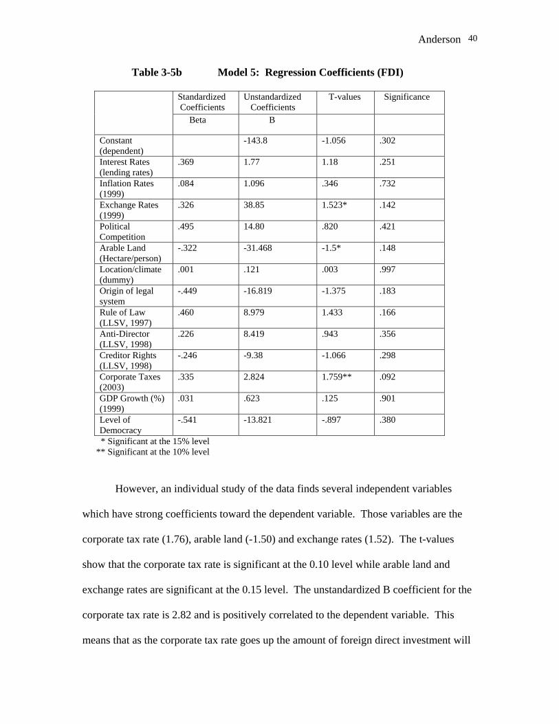
Table 3-5b Model 5: Regression Coefficients (FDI)




Beta B


-143.8 -1.056 .302


.369

1.77 1.18 .251


.084 1.096 .346 .732


.326 38.85 1.523* .142


.495 14.80 .820 .421


-.322 -31.468 -1.5* .148


.001 .121 .003 .997


-.449 -16.819 -1.375 .183


.460 8.979 1.433 .166


.226

8.419 .943 .356


-.246 -9.38 -1.066 .298


.335 2.824 1.759** .092


.031 .623 .125 .901

Level of Democracy

-.541 -13.821 -.897 .380

* Significant at the 15% level ** Significant at the 10% level

However, an individual study of the data finds several independent variables

which have strong coefficients toward the dependent variable. Those variables are the

corporate tax rate (1.76), arable land (-1.50) and exchange rates (1.52). The t-values

show that the corporate tax rate is significant at the 0.10 level while arable land and

exchange rates are significant at the 0.15 level. The unstandardized B coefficient for the

corporate tax rate is 2.82 and is positively correlated to the dependent variable. This

means that as the corporate tax rate goes up the amount of foreign direct investment will

Anderson 41

increase by 2.82 for each percentage increase. The Beta value for this variable is 0.335,

which is the strongest Beta of the significant variables. This value shows that corporate

tax rates explain over one-third of the variance in the dependent variable. The

unstandardized B coefficient for arable land is –31.47. This variable is negatively

correlated to foreign direct investment, which means that a country with a small amount

of arable land will have greater amounts of foreign direct investment. The Beta value for

arable land is -.322, which is almost as strong as the corporate tax variable. The

unstandardized B coefficient for the exchange rates variable is positively correlated at

38.85. This means that a country with stronger exchange rates, in comparison with the

US dollar, have more foreign direct investment. The Beta value for this variable is .326,

and this variable like the other two explains roughly the same amount of variance in the

dependent variable.

Conclusions & Implications

Only one of the five models returned an F-statistic that was significant (model 3).

The other models have a high probability that chance factors are manipulating the model.

The R-square values were less than I had expected. An explanation for this could be the

competition between the thirteen variables, where some variables, due to their strong

Beta values were able to drive out other possibly significant variables. The competition

between the variables seemed to have the designated affect, pushing the weaker variables

to the bottom while the strongest determinants became evident. Though in some cases, a

weaker significance level of 0.15 was used, the sparseness of data required some

concessions at that point. In all cases, I have tried to use data from 1999, however I was

Anderson 42

not always successful, and other newer data were used to supplement the data from 1999.

This may have produced some of the different results within this study.

After examining the statistically significant values in each model, one point

becomes clear. The separate independent variables for the monetary & fiscal policy

hypothesis seem to show a strong correlation in each of the models except the first.

More monetary & fiscal policy variables were associated with the dependent variables

then were the legal, endowment and political theories. This analysis validates the

hypothesis that monetary and fiscal policy affects the strength of capital markets. The

analysis also validates the previous studies that found that endowment and law theories

are active in determining the strength of capital markets, and that the politics variables

seemed to have little affect on the strength of capital markets. However, I do feel that

politics still does play a role in determining the strength of capital markets; it might just

be an indirect role, as is suggested by others. These results fall into line with the research

already completed by various authors in regards to politics, law, endowment, and finance.

I hope that this will add to the increasing evidence on the strength of capital markets.

The research conducted in this study provides a new set of variables to examine

market strength. The strong connection between the various proxies (dependent

variables) for market strength and the corporate tax rate, inflation rate, interest rate

variables show that the strength of capital markets can be explained through other

avenues rather than looking specifically at the legal and endowment theories. The legal

and endowment theories help to explain the constant factors that are shown in strong

capital markets. Looking at the rule of law, origin of the legal system, rights, amount of

land and location, each of these are extremely difficult to change, and therefore they

Anderson 43

cannot provide any practical applications for change. The most practical way to

strengthen a capital market can be seen in the hypothesis I have utilized in this paper.

The empirical results show that inflation, interest rates, corporate taxes and exchange

rates all contribute to the strength of capital markets. This is an important discovery

because a government institution can easily manipulate these variables, in order to

facilitate a stronger capital market. However, the foundation must be set through the

laws of society (the rule of law and specific rights for investors) because investment

protection is still a very important aspect of capital market strength.

Anderson 44

Works Cited Acemoglu, Daron, Johnson, Simon, and Robinson, James. (2001) “Reversal of Fortune:

Geography and Institutions in the Making of Modern World Income Distribution.” MIT, Department of Economics Working Paper 01-38.

Beck, Thorsten, Demirguc-Kunt, Asli, and Levine, Ross. (2001) “Law, Politics, and

Finance.” World Bank, Working Paper. Easterly, William, and Levine, Ross. (2002) “Tropics, Germs, and Crops: How

Endowments Influence Economic Development.” Center for Global Development, Working Paper, No.9.

Frankel, Jeffrey and Romer, David. (1999) “Does Trade Cause Growth,” The American

Economic Review. 89: 379-399. Goldsmith, Raymond. (1969) Financial Structure and Development. New Haven:

Colonial Press Inc. Haber, Stephen. (1991) “Industrial Concentration and the Capital Markets: A

Comparative Study of Brazil, Mexico and the United States, 1830-1930.” Journal of Economic History. 50: 559-580.

Hausmann, Ricardo. (2001) “Prisoners of Geography.” Foreign Policy. February: 45-53. Keynes, John Maynard. (1936) The General Theory of Employment, Interest and Money.

New York: Harcourt, Brace and Company. King, Robert & Levine, Ross. (1993) “Finance and Growth: Schumpeter Might be

Right.” Quarterly Journal of Economics. 108: 717-738. La Porta, Rafael, Lopez-de-Silanes, Florencio, Shleifer, Andrei, and Vishny, Robert.

(1998) “Law and Finance.” Journal of Political Economy. 106: 1113-1154. La Porta, Rafael, Lopez-de-Silanes, Florencio, Shleifer, Andrei, and Vishny, Robert.

(1997) “Legal Determinants of External Finance.” The Journal of Finance. 52: 1131-1150.

Levine, Ross. (1991) “Stock Markets, Growth, and Tax Policy.” The Journal of Finance.

46: 1445-1459. McKinnon, Ronald. (1973) Money and Capital in Economic Development. The

Brookings Institution: Washington D.C. Meek, Thomas. (1960) “The Revival of International Capital Markets.” American

Economic Review. 50: 282-293.

Anderson 45

Meltzer, Allan H. (1990) Keynes Monetary Theory. New York: Cambridge University

Press. Modigliani, Franco and Miller, Merton. (1958) “The Cost of Capital, Corporation

Finance and the Theory of Investment.” The American Economic Review, 48: 261-297.

Montesquieu, Baron Charles De Secondat. (1748) The Spirit of Laws. Book XXI:

Chapter 11. North, Douglass. (1991) Institutions, Institutional Change and Economic Performance.

New York: Cambridge University Press. Olson, Mancur. (1993) “Dictatorship, Democracy, and Development,” American Political

Science Review. 87: 567-576. Smith, Adam. (1776, 1911) An Inquiry into the Nature and Causes of the Wealth of

Nations. London: J.M. Dent & Sons. Vol. I & II.

Capital Markets: Monetary and Fiscal Policy … Markets: Monetary and Fiscal Policy Determinants ......

Documents

Transcript of Capital Markets: Monetary and Fiscal Policy … Markets: Monetary and Fiscal Policy Determinants ......